Level set method for the inverse elliptic problem in

nonlinear electromagnetism

Ivan Cimrak1, Roger Van Keer

NaM2 Research Group, Department of Mathematical Analysis, Ghent University,

Galglaan 2, B-9000 Ghent, Belgium

Abstract

An inverse problem of inhomogeneity identification inside a nonlinear mag-netic material from the local measurements of the magnetic induction isinvestigated. The representation of the shape of the inhomogeneity and itsevolution during an iterative reconstruction process is achieved by the levelset method. The reconstruction is realized by the minimization of a cost func-tion using the steepest descent method. The gradient directions are evaluatedusing the sensitivity equation and the adjoint variable method. Simulationshas been performed showing the robustness of the algorithm and its abil-ity to reconstruct single inhomogeneities, convex and non-convex, as well asmultiple inhomogeneities.

Keywords: sensitivity analysis, adjoint problem, shape optimization, levelset method2008 MSC: 35R30, 65M32

1. Introduction

We model physical processes governed by quasi-linear equations wherethe properties of the material are described by piecewise smooth functions.

Email addresses: ivan.cimrak@ugent.be (Ivan Cimrak), roger.vankeer@ugent.be(Roger Van Keer)

URL: cage.ugent.be/~cimo (Ivan Cimrak), cage.ugent.be/~rvk (Roger VanKeer)

1Ivan Cimrak is supported by the Fund for Scientific Research - Flanders FWO, Bel-gium.

Preprint submitted to Journal of Computational Physics August 31, 2010

Such description includes electromagnetic processes with nonlinear magneticmaterials. More specifically, electromagnetic non-destructive evaluation aimat e.g. the localization of crack or inhomogeneities in the steel productionprocess and these impurities can be described by piecewise smooth functions.

Non-destructive evaluation has gained a lot of interest during the lastdecade, since it is becoming an important tool in different research topics.Eddy current testing has been widely used for defects characterization inmaterials [1]. We aim at developing a numerical technique capable of propercharacterization of defects in magnetically non-linear materials. Althoughthe linear model used in the EIT is sometimes sufficient for the acceptabledefect detection, the non-linear model introduced in the following sectionis more robust and able to reconstruct the shape of the crack or of theinhomogeneity even in the cases when the linear model is not. The superiorityof the non-linear model is evident especially in the cases when measurementsare not given over the whole workpiece but only at the part of it, mostlyaround the boundary. In that cases the linear model is not accurate enoughto reconstruct the crack inside the material from the measurements near theboundary. The non-linear model reliably detects this air-gaps.

The paper is organized as follows. In Section 2 we describe the model andits mathematical description. In Section 3 we describe the level set methodthat is used in the representation of the unknown shapes. Then we analyzethe direct problem in Section 4 and we define the inverse problem in Section5. The inverse problem is solved by means of minimization of a cost function.Here we derive the sensitivity equation and the adjoint problem that togethergives an explicit expression for the derivative of the cost function.

Section 6 is devoted to numerical simulations. We describe the algorithmand we test it for several scenarios including the determination of convex,non-convex and multiple cracks. Finally in Section 7 we draw several con-clusions.

2. Model description

Suppose that the bounded domain Ω ∈ R2 with C1 boundary contains

a subdomain D ∈ R2, possibly not connected. Assume that the function

ν : Ω × R → R is defined piecewise by

ν(x, s) =

ν1(s) for x ∈ D,ν2(s) for x ∈ Ω \D

(1)

2

y

x

ΩΩ \D

D = airgap

= steel

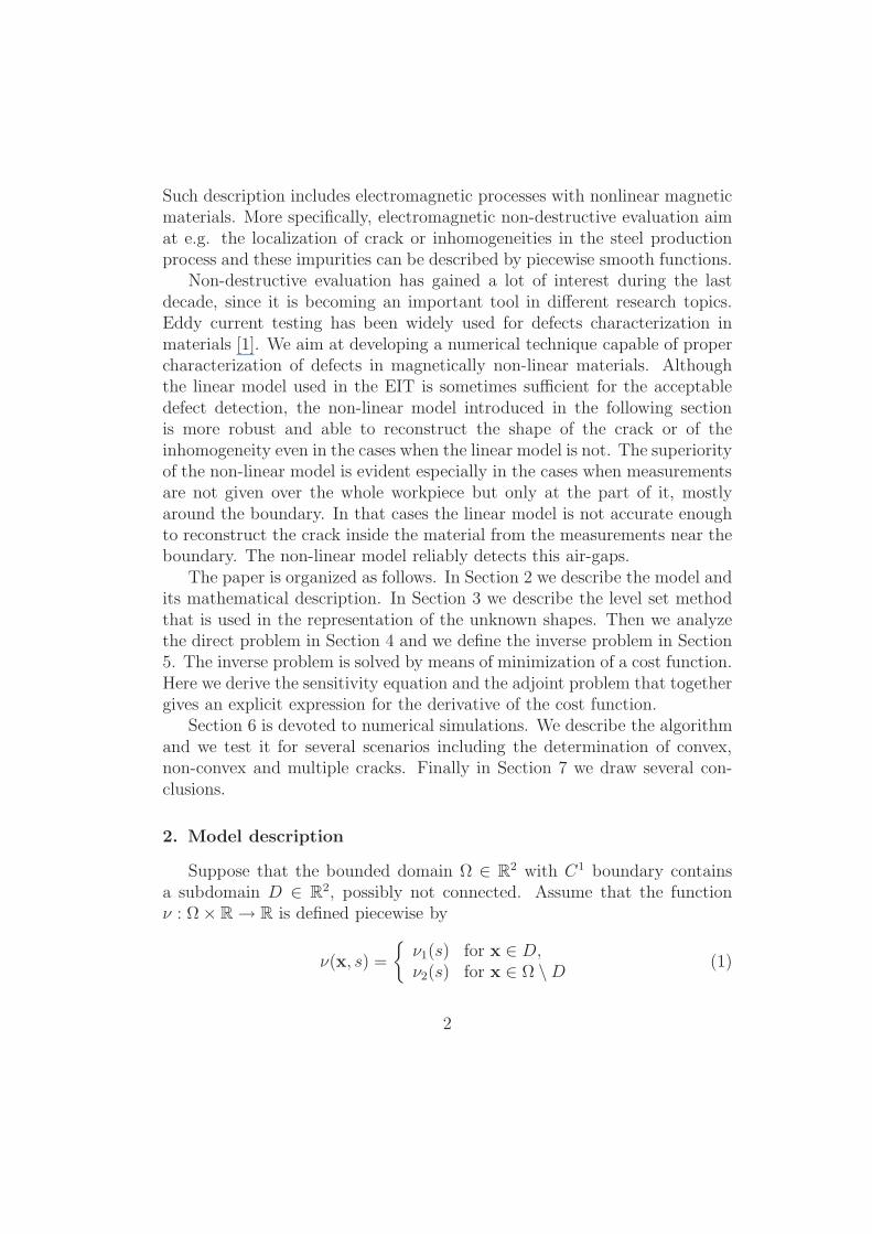
Figure 1: The geometry of the problem consists of a bounded domain Ω. The workpieceoccupies the whole domain, the air gap D excluded. The computational domain Ω is thussplit into two non-overlapping subdomains Ω \D and D.

where ν1, ν2 are nonlinear functions.The direct problem is governed by the following quasi-linear partial dif-

ferential equation

∇ · (ν(x, |∇A|2)∇A) = J in Ω, A = 0 on ∂Ω (2)

with J being a suitable function. Since ν is discontinuous across the boundary∂D we work with weak formulation of the problem.

The above mathematical model covers many physical and industrial ap-plications. For a linear choice of ν1 and ν2, the problem (2) describes the EITproblem [2, 3, 4, 5, 6]. For a nonlinear ν2 the model describes the followingelectromagnetic problem.

The workpiece made of hard magnetic steel has a crack inside it. Thecrack is filled with air. By a function J one can model the current density thatinduces a magnetic field. In this setting, two materials occur, the air and thesteel, with respective permeabilities µ1, µ2. The magnetic permeability µ(x)as a space variable function defined in the whole Ω has thus value µ1 insideD, and value µ2 in Ω \D. It has therefore a discontinuity at the boundaryof D. We are interested in the static distribution of the magnetic field underthe induced current density J.

The electromagnetic process in the above example is governed by thestatic magnetic vector potential formulation of the Maxwell equations with

3

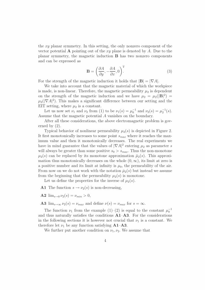
the xy planar symmetry. In this setting, the only nonzero component of thevector potential A pointing out of the xy plane is denoted by A. Due to theplanar symmetry, the magnetic induction B has two nonzero componentsand can be expressed as

B =

(

∂A

∂y,−

∂A

∂x, 0

)T

. (3)

For the strength of the magnetic induction it holds that |B| = |∇A|.We take into account that the magnetic material of which the workpiece

is made, is non-linear. Therefore, the magnetic permeability µ2 is dependenton the strength of the magnetic induction and we have µ2 = µ2(|B|2) =µ2(|∇A|

2). This makes a significant difference between our setting and theEIT setting, where µ2 is a constant.

Let us now set ν1 and ν2 from (1) to be ν1(s) = µ−10 and ν2(s) = µ−1

2 (s).Assume that the magnetic potential A vanishes on the boundary.

After all these considerations, the above electromagnetic problem is gov-erned by (2).

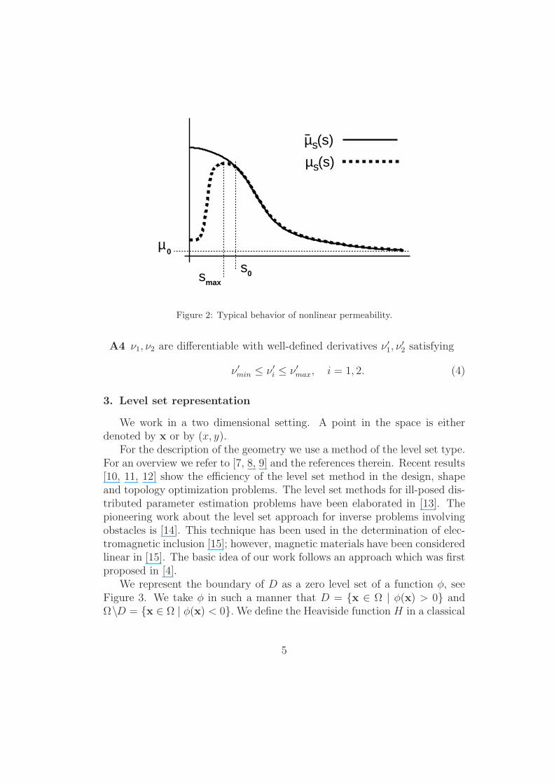
Typical behavior of nonlinear permeability µ2(s) is depicted in Figure 2.It first monotonically increases to some point smax where it reaches the max-imum value and then it monotonically decreases. The real experiments wehave in mind guarantee that the values of |∇A|2 entering µ2 as parameter swill always be greater than some positive s0 > smax. Thus the non-monotoneµ2(s) can be replaced by its monotone approximation µ2(s). This approxi-mation thus monotonically decreases on the whole (0,∞), its limit at zero isa positive number and its limit at infinity is µ0, the permeability of the air.From now on we do not work with the notation µ2(s) but instead we assumefrom the beginning that the permeability µ2(s) is monotone.

Let us define the properties for the inverse of µ2(s).

A1 The function s→ ν2(s) is non-decreasing,

A2 lims→0 ν2(s) = νmin > 0,

A3 lims→∞ ν2(s) = νmax and define ν(s) = νmax for s = ∞.

The function ν1 from the example (1)–(2) is equal to the constant µ−10

and thus naturally satisfies the conditions A1–A3. For the considerationsin the following sections it is however not crucial that ν1 is a constant. Wetherefore let ν1 be any function satisfying A1–A3.

We further put another condition on ν1, ν2. We assume that

4

µ (s)s

µ (s)s

0µ

smax

s0

Figure 2: Typical behavior of nonlinear permeability.

A4 ν1, ν2 are differentiable with well-defined derivatives ν ′1, ν′

2 satisfying

ν ′min ≤ ν ′i ≤ ν ′max, i = 1, 2. (4)

3. Level set representation

We work in a two dimensional setting. A point in the space is eitherdenoted by x or by (x, y).

For the description of the geometry we use a method of the level set type.For an overview we refer to [7, 8, 9] and the references therein. Recent results[10, 11, 12] show the efficiency of the level set method in the design, shapeand topology optimization problems. The level set methods for ill-posed dis-tributed parameter estimation problems have been elaborated in [13]. Thepioneering work about the level set approach for inverse problems involvingobstacles is [14]. This technique has been used in the determination of elec-tromagnetic inclusion [15]; however, magnetic materials have been consideredlinear in [15]. The basic idea of our work follows an approach which was firstproposed in [4].

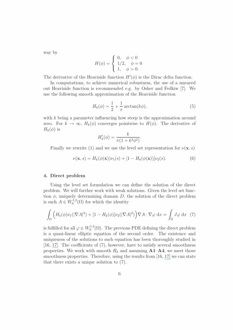
We represent the boundary of D as a zero level set of a function φ, seeFigure 3. We take φ in such a manner that D = x ∈ Ω | φ(x) > 0 andΩ\D = x ∈ Ω | φ(x) < 0. We define the Heaviside function H in a classical

5

way by

H(φ) =

0, φ < 01/2, φ = 01, φ > 0.

The derivative of the Heaviside function H ′(φ) is the Dirac delta function.In computations, to achieve numerical robustness, the use of a smeared

out Heaviside function is recommended e.g. by Osher and Fedkiw [7]. Weuse the following smooth approximation of the Heaviside function

Hk(φ) =1

2+

1

πarctan(kφ), (5)

with k being a parameter influencing how steep is the approximation aroundzero. For k → ∞, Hk(φ) converges pointwise to H(φ). The derivative ofHk(φ) is

H ′

k(φ) =k

π(1 + k2φ2).

Finally we rewrite (1) and we use the level set representation for ν(x, s)

ν(x, s) = Hk(φ(x))ν1(s) + [1 −Hk(φ(x))]ν2(s). (6)

4. Direct problem

Using the level set formulation we can define the solution of the directproblem. We will further work with weak solutions. Given the level set func-tion φ, uniquely determining domain D, the solution of the direct problemis such A ∈W 1,2

0 (Ω) for which the identity

∫

Ω

(

Hk(φ)ν1(|∇A|2) + [1 −Hk(φ)]ν2(|∇A|

2))

∇A · ∇ϕ dx =

∫

Ω

Jϕ dx (7)

is fulfilled for all ϕ ∈W 1,20 (Ω). The previous PDE defining the direct problem

is a quasi-linear elliptic equation of the second order. The existence anduniqueness of the solutions to such equation has been thoroughly studied in[16, 17]. The coefficients of (7), however, have to satisfy several smoothnessproperties. We work with smooth Hk and assuming A1–A4, we meet thosesmoothness properties. Therefore, using the results from [16, 17] we can statethat there exists a unique solution to (7).

6

-0.4-0.2

0 x-0.4

-0.3

-0.2

-0.20.2

y

-0.1

0

0

0.2

0.1

0.4

0.2

0.4

Figure 3: Level set function φ. The intersection of the surface z = φ(x, y) with the planez = 0 forms the circle representing the boundary of D.

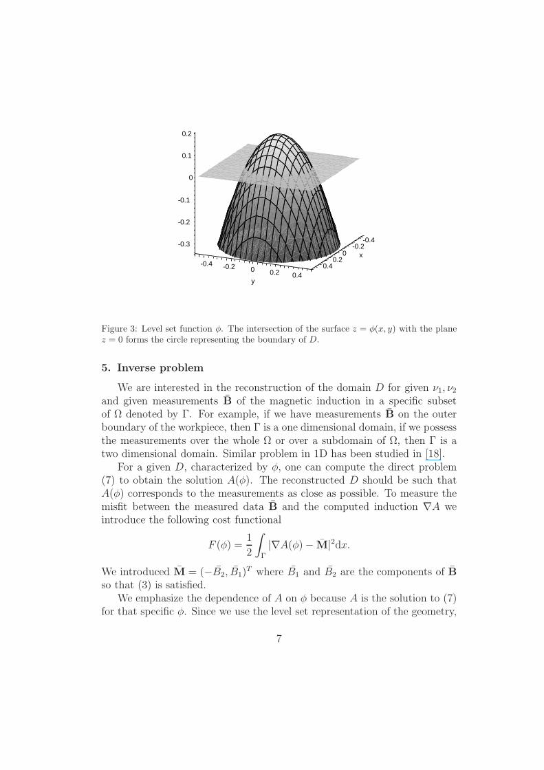
5. Inverse problem

We are interested in the reconstruction of the domain D for given ν1, ν2

and given measurements B of the magnetic induction in a specific subsetof Ω denoted by Γ. For example, if we have measurements B on the outerboundary of the workpiece, then Γ is a one dimensional domain, if we possessthe measurements over the whole Ω or over a subdomain of Ω, then Γ is atwo dimensional domain. Similar problem in 1D has been studied in [18].

For a given D, characterized by φ, one can compute the direct problem(7) to obtain the solution A(φ). The reconstructed D should be such thatA(φ) corresponds to the measurements as close as possible. To measure themisfit between the measured data B and the computed induction ∇A weintroduce the following cost functional

F (φ) =1

2

∫

Γ

|∇A(φ) − M|2dx.

We introduced M = (−B2, B1)T where B1 and B2 are the components of B

so that (3) is satisfied.We emphasize the dependence of A on φ because A is the solution to (7)

for that specific φ. Since we use the level set representation of the geometry,

7

the inverse problem is defined as follows: Find the level set function φ forwhich the cost function F (φ) is minimal, i.e. find φmin ∈W 1,2(Ω) such that

φmin = arg minφ∈W 1,2(Ω)

F (φ). (8)

To this end we employ a gradient-type minimization method to minimizethe cost function. For this we need to compute the gradient DF of F withrespect to φ.

We introduce the notation for the Gateaux derivative of an arbitraryfunction f(φ) in the direction h

δh(f) = δh(f(φ)) =df(φ)

dφh.

In order to compute the gradient of F with respect to φ we first compute theGateaux derivative in the direction h

δh(F ) = limε→∞

F (φ+ εh) − F (φ)

ε=

∫

Γ

∇δh(A) · (∇A(φ) − M)dx. (9)

We will use a finite element method for the finite dimensional approx-imation of φ. We choose Lagrange finite elements of the first order. Thishowever means that if the mesh has N vertices, the parameter space willhave N degrees of freedom. Thus, for the full gradient of F one needs tocompute δhA for h = ϕ1, . . . ϕN , where ϕi are the basis functions of our finiteelement space. Once we know δϕi

F , the gradient will be expressed as

DF =N

∑

i=1

δϕiFϕi. (10)

For the computation of the gradient we use the adjoint variable method.A similar approach of an adjoint variable has been used in many applications[19, 20, 21, 22, 23, 24]. We choose this method because of its computationalcost reduction in comparison with the conventional method of perturbationsor with the method of sensitivity equation. This speed up is caused by thefact that the direct problem is nonlinear and therefore it must be solvediteratively.

To obtain δh(F ), we use (9) and thus we formally differentiate the directproblem (7). We get the following sensitivity equation

∫

Ω

δh[ν(x, |∇A|2)]∇A · ∇ϕ dx+

∫

Ω

ν(x, |∇A|2)∇δhA · ∇ϕ dx = 0

8

We start with the first term. We must still keep in mind that A is dependenton φ.

δh[ν(x, |∇A|2)] = δh[Hk(φ)](ν1(|∇A|

2) − ν2(|∇A|2)) (11)

+2Hk(φ)ν ′1(|∇A|2)∇δhA · ∇A

+2[

1 −Hk(φ)]

ν ′2(|∇A|2)∇δhA · ∇A(φ).

Further we computeδh[Hk(φ)] = H ′

k(φ)h.

Finally, putting all particular results together we write down the sensitivityequation

∫

Ω

2(

Hk(φ)ν ′1(|∇A|2) + [1 −Hk(φ)]ν ′2(|∇A|

2))

∇δhA · ∇A∇A · ∇ϕ dx

+

∫

Ω

(

Hk(φ)ν1(|∇A|2) + [1 −Hk(φ)]ν2(|∇A|

2))

∇δhA · ∇ϕ dx

= −

∫

Ω

H ′

k(φ)h(

ν1(|∇A|2) − ν2(|∇A|

2))

∇A · ∇ϕ dx. (12)

To avoid the computation of δhA from (12) for h = ϕi, i = 1, . . . , N weintroduce the adjoint variable b being the solution of the following problem

∫

Ω

2(

Hk(φ)ν ′1(|∇A|2) + [1 −Hk(φ)]ν ′2(|∇A|

2))

∇b · ∇A∇A · ∇ψ dx

+

∫

Ω

(

Hk(φ)ν1(|∇A|2) + [1 −Hk(φ)]ν2(|∇A|

2))

∇b · ∇ψ dx

=

∫

Γ

(∇A(φ) − M) · ∇ψ dx. (13)

Now, we take special test functions in the weak formulation of the sensi-tivity equation and of the equation for the adjoint variable. Take ϕ = b in(12) and ψ = δhA in (13). We see that the left-hand sides of (12) and (13)are equal. Hence, we get the equality of the right-hand sides

−

∫

Ω

H ′

k(φ)h[ν1(|∇A|2)−ν2(|∇A|

2)]∇A ·∇b dx =

∫

Γ

(∇A(φ)−M) ·∇δhA dx.

The adjoint problem was constructed in such a way that the right-hand sideof the above expression is exactly the Gateaux derivative of F with respect

9

to φ in the direction h. Eventually we obtained

δhF = −

∫

Ω

H ′

k(φ)h(

ν1(|∇A|2) − ν2(|∇A|

2))

∇A · ∇b dx, (14)

where A is the solution to the direct problem (7) and b is the solution of theadjoint problem (13).

Here we see why we need to use a smeared-out Heaviside function. Theprevious integral in its non-smeared-out form represents an integral overlower-dimensional interface and it is unlikely that any standard numericalapproximation based on sampling will give a good approximation to thisintegral.

Next, we have two possibilities: either we compute N integrals to obtainδϕiF for i = 1, . . . , N and then from (10) we obtainDF , or, we simply project

H ′

k(φ)[ν1(|∇A|2)−ν2(|∇A|

2)]∇A ·∇b onto the finite element space by solvingthe following linear equation

−

∫

Ω

H ′

k(φ)[ν1(|∇A|2) − ν2(|∇A|

2)]∇A · ∇bϕ dx =

∫

Ω

DFϕ dx (15)

with the unknown DF . Simulations confirm that the second choice is faster.

6. Numerical implementation

Throughout this section we consider Ω ∈ R2 to be a square (−0.5, 0.5)×

(−0.5, 0.5). We assume that we possess the measurements over the whole Ω.The direct problem (7) can be seen as an operator equation G(A) = J whereG is a mapping G : A ∈W 1,2

0 (Ω) → G(A) ∈W 1,20 (Ω) such that

∫

Ω

(

Hk(φ)ν1(|∇A|2) + [1 −Hk(φ)]ν2(|∇A|

2))

∇A · ∇ϕ dx =

∫

Ω

G(A)ϕ dx.

This operator equation is nonlinear and therefore it will be solved for allthe numerical examples by the same iterative algorithm. Starting from theinitial guess A0, we use the Newton-Raphson algorithm based on the followingupdate

Ai+1 = Ai − [DG(Ai)]−1(G(Ai) − J).

Notice that for each iteration one linear PDE has to be solved.The material parameter functions ν1, ν2 are chosen in such a way that

they mimic the real setting described in the Introduction. ν1 is a constant

10

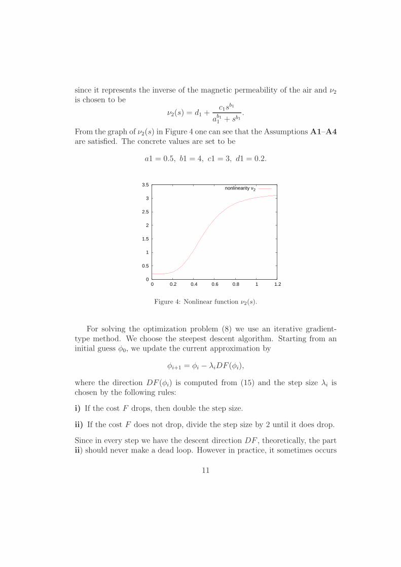
since it represents the inverse of the magnetic permeability of the air and ν2

is chosen to be

ν2(s) = d1 +c1s

b1

ab11 + sb1

.

From the graph of ν2(s) in Figure 4 one can see that the Assumptions A1–A4are satisfied. The concrete values are set to be

a1 = 0.5, b1 = 4, c1 = 3, d1 = 0.2.

0

0.5

1

1.5

2

2.5

3

3.5

0 0.2 0.4 0.6 0.8 1 1.2

nonlinearity ν2

Figure 4: Nonlinear function ν2(s).

For solving the optimization problem (8) we use an iterative gradient-type method. We choose the steepest descent algorithm. Starting from aninitial guess φ0, we update the current approximation by

φi+1 = φi − λiDF (φi),

where the direction DF (φi) is computed from (15) and the step size λi ischosen by the following rules:

i) If the cost F drops, then double the step size.

ii) If the cost F does not drop, divide the step size by 2 until it does drop.

Since in every step we have the descent direction DF , theoretically, the partii) should never make a dead loop. However in practice, it sometimes occurs

11

that the computed gradient is not accurate enough and in fact it is not adescent direction any more. Therefore, we sometimes proceed against thedescent direction in order to get to a more stable area.

Initially, all simulations featured oscillations of the zero level set. Tostabilize the optimization process we introduce the regularization and we adda Tikhonov stabilizing term. We choose the squared norm of the gradient ofthe level set function. We use the coefficient α to control the trade-off betweenthe fidelity term and the regularizing term. The resulting cost function readsas

F (φ) =1

2

∫

Γ

|∇A(φ) − M|2dx+ α

∫

Ω

|∇φ|2dx.

The expression for the Gateaux derivative of F with respect to φ in thedirection h will be derived from (14) by adding the corresponding derivativeof the regularization term leading to

δhF = −

∫

Ω

H ′

k(φ)h[ν1(|∇A|2)−ν2(|∇A|

2)]∇A·∇b dx+2α

∫

Ω

∇h·∇φdx. (16)

The linear problems are solved on the regular triangular mesh with 2dim2

triangles constructed by splitting of the square into dim2 small squares andnext splitting each of them into two triangles.

It is often the case that in the iteration process the level set functionbecome too steep or too flat around its zero level set. This causes difficultiesand errors in determination of the zero level set. To overcome this drawback,a re-initialization is frequently used. This means that if the norm of ∇φi

becomes too high or too small around the zero level set of φi, then φi isreset to the distance function with respect to its zero level set [7]. Severalstrategies without using re-initialization have been described in [25].

We however do not need to use re-initialization. During the simulationswe regularly check the value |∇φi| around the interface and it always remainsbetween 0.7 and 3 which is acceptable.

We design three numerical examples with different exact shapes in orderto demonstrate the convergence of the adjoint variable method implementedto solve the optimization problem (8). The first example shows how thealgorithm finds the exact circular shape from the initial ellipsoidal shape.The second example tests the algorithm on a more complicated non-convexshrimp-like exact shape. The third numerical example covers the case of anexact shape consisting of several large disjoint parts.

12

To quantify the convergence of the method we introduce a distance be-tween two shapes. Since any shape is represented by a zero level set of a levelset function, we define the distance dist(φ1, φ2) between two shapes using itslevel set representations φ1, φ2 in the following way

dist(φ1, φ2) = ‖Hk(φ1) −Hk(φ2)‖L2(D)

and we say that the sequence of shapes represented by φn converges to ashape represented by φ iff dist(φn, φ) → 0. Notice, that we can manipulatewith the distance by changing the value of k. Indeed, regardless what valueof k has been used in the determination of the shape, for the measuringof the obtained shape we can use a different k. The higher k means thatthe interface is sharper and therefore two different shapes are distinguishedbetter.

0.001

0.01

0.1

1

10

100

1 10 100 1000

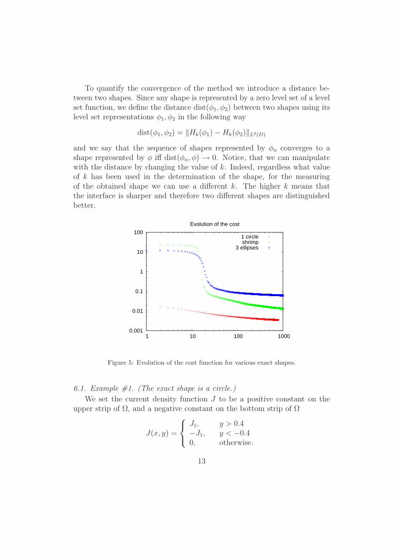
Evolution of the cost

1 circleshrimp

3 ellipses

Figure 5: Evolution of the cost function for various exact shapes.

6.1. Example #1. (The exact shape is a circle.)

We set the current density function J to be a positive constant on theupper strip of Ω, and a negative constant on the bottom strip of Ω

J(x, y) =

J1, y > 0.4−J1, y < −0.40, otherwise.

13

0.001

0.01

0.1

1

1 10 100 1000

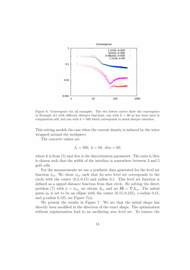
Convergence

1 circle, k=500shrimp, k=500

3 ellipses, k=5001 circle, k=80

Figure 6: Convergence for all examples. The two lowest curves show the convergencein Example #1 with different distance functions, one with k = 80 as has been used incomputation self, and one with k = 500 which corresponds to much sharper interface.

This setting models the case when the current density is induced by the wireswrapped around the workpiece.

The concrete values are

J1 = 500, k = 80, dim = 60,

where k is from (5) and dim is the discretization parameter. The ratio k/dimis chosen such that the width of the interface is somewhere between 3 and 5grid cells.

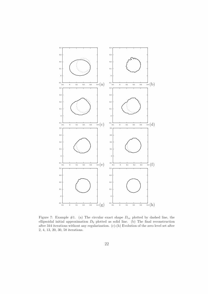
For the measurements we use a synthetic data generated for the level setfunction φex. We chose φex such that its zero level set corresponds to thecircle with the center (0.2, 0.15) and radius 0.1. This level set function isdefined as a signed distance function from that circle. By solving the directproblem (7) with φ = φex, we obtain Aex and set M = ∇Aex. The initialguess φ0 is set to be an ellipse with the center (0.15, 0.125), x-radius 0.15,and y-radius 0.125, see Figure 7(a).

We present the results in Figure 7. We see that the initial shape hasdirectly been modified in the direction of the exact shape. The optimizationwithout regularization lead to an oscillating zero level set. To remove the

14

oscillations we use the Tikhonov regularization with coefficient α = 0.01.Eventually, the optimization process ends up finding the exact shape.

6.2. Example #2. (The exact shape has a shrimp-like form.)

In this numerical example and also in the examples #3 and # 4 we takethe values

J1 = 500, k = 60, dim = 40,

and the current density function J to be a positive constant J1 over the wholeΩ.

In the example #2 we choose for the exact domain a more exotic shrimp-like shape. The initial guess φ0 is set to be a circle inside the shrimp withthe center (0.0, 0.1), and radius 0.05, see Figure 8(a).

We use the Tikhonov regularization with coefficient α = 0.02.The evolution of the zero level set is depicted in Figure 8. We see that

during the iterations 0–16 the initial small circle gets larger and maintainsthe circular shape until it hits the borders of the exact shape. Then, until theiteration 19 it adapts to the shrimp-like shape and the rest of the evolutionis simply an adjustment to fit the exact shape.

In Figure 5 we see a significant drop in the value of the cost. The dropappears in between the iterations 15 and 20. That precisely corresponds tothe phase when the approximating shape hits the borders of the exact shapeand tries to adjust to the shrimp-like form.

6.3. Example #3. (The exact shape consists of three large ellipses.)

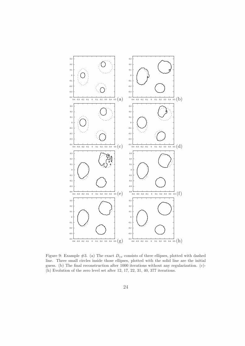
To test the ability of the algorithm to detect disconnected regions wechoose three ellipses as the exact shape. The constants J1, k and dim areset as in Example #2. We use the Tikhonov regularization with coefficientα = 0.1.

The evolution of the zero level set can be seen in Figure 9. Three smallinitial circles uniformly grow until they hit the borders of the exact ellipses,see the iterations 0–17. The upper right circle covers approximately only onehalf of the exact ellipse. Then the approximate circles almost fill the exactellipses, see iterations 17–40 and afterwards, the algorithm just fine-tunesthe exact shape.

Again, we can see this behavior in Figure 5. The cost lowers its valueslightly during the iterations 0–17, then it suddenly drops and after theiteration 40 it goes down again slightly.

15

6.4. Convergence

The convergence of the methods for all three examples is depicted inFigure 6. We plotted dist(φn, φex) against the number of iterations n. As wasalready mentioned at the end of Section 5, the use of smeared-out Heavisidefunction in the simulations is needed since the integral in (14) is taken overa lower-dimensional interface. However, the distance function dist(φn, φex) isdefined as an integral over the whole domain. Therefore to better distinguishbetween two shapes, a sharper interface is more suitable. We thus use a higherk for the evaluation of the distance, namely we take k = 500.

We see that the convergence curves in Figure 6 and the curves for theevolution of the cost functional in Figure 5 are very similar.

The behavior of two convergence curves for Example #1 (for k = 500 andfor k = 80) shows an interesting phenomenon. Around the 60th iteration,the value of the distance function dist(φn, φex) is the lowest and later on, thisdistance even slightly raises. Graphically, the approximating shape coincideswith the exact shape just around the 60th iteration and thereafter bothshapes remain identical. The reason for the raise of the distance dist(φn, φex)for n > 60, is that the distance function is an integral over the whole domainand with further evolution of φ, φn can differ from φex on the locationsoutside the interface and thus the distance can raise (in Example #1) evenif the shapes remain identical. In other two examples, the distance functiondecreases during the whole evolution.

The evolution of φn for n > 60 is driven by the gradient DF whichminimizes F , since the interface is not sharp. The zero level set howeverdoes not change.

This phenomenon is diminished by using a higher k in the distance func-tion dist(φn, φex) however, the higher k, the more oscillations appear.

6.5. Sensitivity to the noise

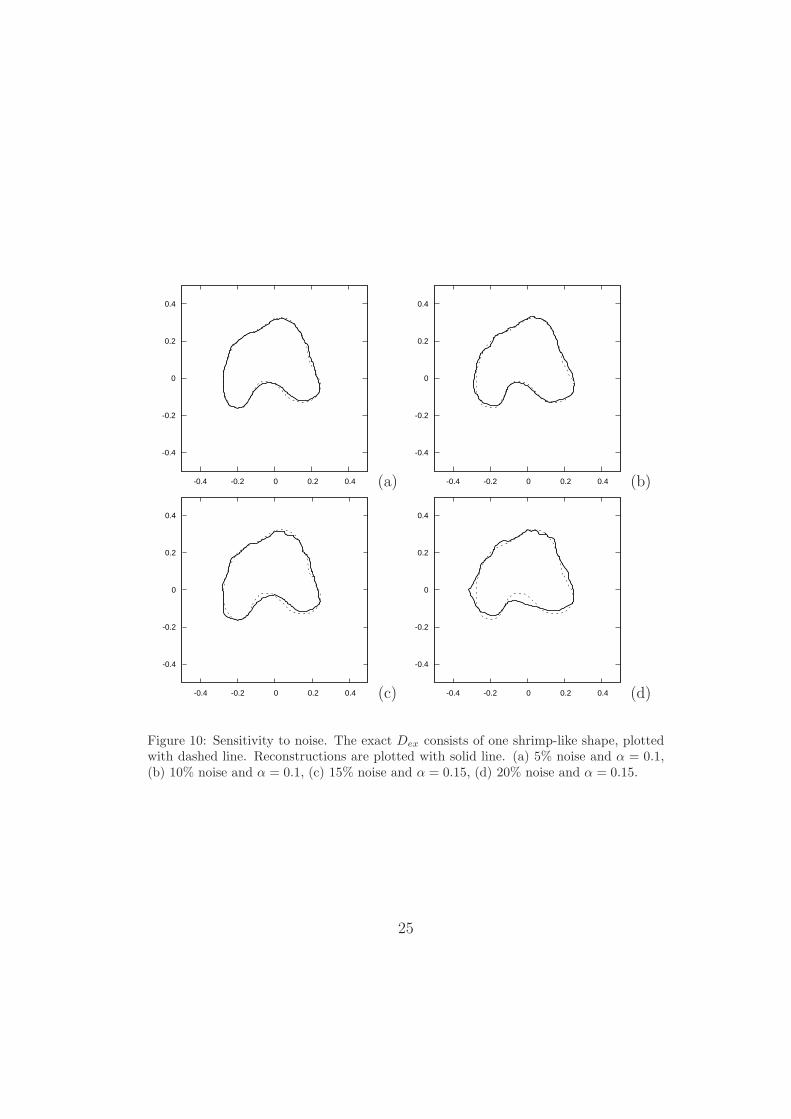
To demonstrate the capability of the algorithm to cope with the noise inthe data we run the following simulation. We use the settings from Example#2. We show four simulations, with data corrupted by the 5%, 10%, 15%and 20%, respectively. The results are depicted in Figure 10. With noiselevels 5% and 10% we used Tikhonov regularization with coefficient α = 0.1.With higher noise level we had to increase the regularization weight to 0.15to obtain non-oscillatory reconstructions. We see that even for quite highnoise levels of 5% and 10%, the algorithm is still able to reconstruct theair-gap with a reasonable accuracy. Of course, the chosen regularization was

16

successful only because of the smooth exact domain. If the exact shape Dex

has sharp corners we will need to use other kinds of regularization such asbounded (or sometimes called total) variation regularization. With 15% and20% noise the reconstruction becomes unacceptable.

6.6. Gradient-for-the-initiation (GFI) method

In the numerical example #1 we set the initial guess to be an ellipsebeing positioned not ”far” from the exact circular shape. In the examples#2 and #3 we set the initial guess to be small circles inside the exact shapes.All this can however be done only in the case that we know the number ofdisconnected regions that form the exact shape. Moreover, we need to knowtheir approximate position too. This is a quite strong assumption and it isalmost never the case that we know this information in advance.

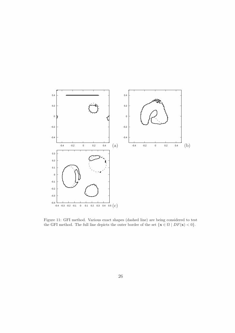
We suggest a heuristic approach how to find the number of the air gapsand their approximate position. We call this approach a Gradient-for-initiationmethod (the GFI method).

Assume that the initial guess for D0 is an empty set. That means that thedomain Ω is completely occupied by the ferromagnetic material without anyair gaps. We compute the cost function for this particular D0. Further wetry to locally remove a tiny amount of the material. Our hypothesis is thatif the material is removed from the places located inside Dex, then the costshould drop and, if the material is removed from the places located outsideDex, the cost will raise.

Assuming our hypothesis is correct, we need to determine those areasleading to the drop of the cost. We do it in the following way. We set thelevel set function φ0 equal to a small negative number. By this we ensurethat D0 = ∅. Further, we set k to be a high positive number so that thesmooth approximation of the Heaviside function is steep around zero. Inthis way we ensure that even a small positive perturbation φδ of φ0 will leadto a nonempty D0+δ = x ∈ Ω | φ0(x) + φδ(x) > 0. Of course, D0+δ will belocated around the support of φδ.

Now we compute the derivative DF of the cost with respect to φ. Thederivative in general has the property that it locally informs how fast thedifferentiated function will raise. That means that in the locations wherethe derivative DF is positive, we can expect the raise of the cost, and in thelocations where it is negative, we can expect the drop of the cost. Therefore,the domain x ∈ Ω | DF (x) < 0 should define a good approximation ofDex.

17

We present the results of the GFI method on three numerical examples inFigures 11 and 12. In Figure 11 the dashed line represents the exact shapewhile the solid line represents the zero level set of the DF . The domainx ∈ Ω | DF (x) < 0 is close to be inside the solid line. We see that thenumber of the air gaps and their approximate position was detected verywell.

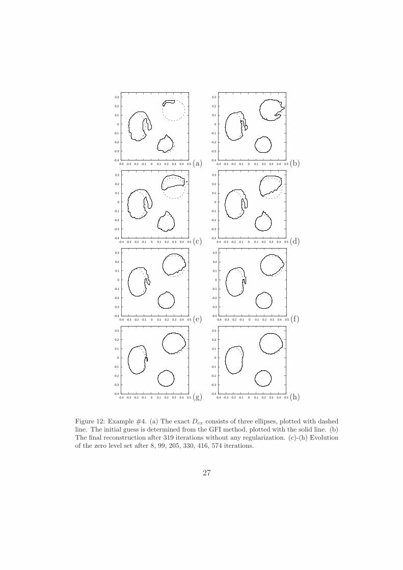
6.7. Example #4

This example shows the result of the optimization when the initial shapehas been determined using the GFI method. The other settings are the sameas in Example #3.

In Figure 12 we see that starting even from a ”wild” initial shape, thealgorithm eventually finds the exact shape.

7. Conclusions

We have implemented a level set method to compute the quasi-linear el-liptic equation describing the magnetic processes inside a nonlinear magneticmaterial that contains air gaps or cracks. In this way we obtained an efficientsolver for the non-linear direct problem.

Furthermore, we solved the inverse problem for the determination of theseair gaps by minimization of the cost function that was defined using themeasurements of the magnetic induction. During the solution process wehad to overcome several difficulties. For the iterative procedure based on thegradient-type minimization algorithms we implemented the adjoint variablemethod. This method brings a tremendous reduction of the computationalcosts in the computation of the gradient direction compared to the classicalperturbation methods.

We tested the algorithm in several numerical examples. We successfullycomputed the inverse problems for three different exact shapes. In eachcase the algorithm found a very close approximation of the exact shape.The three exact shapes with different topological properties were devised totest the algorithm. We tested non-convex domains in the example #2 anddisconnected large regions in the example #3.

Finally, we designed a heuristic algorithm called the Gradient-for-initiationmethod to find a good initial shape for the optimization algorithm. The GFImethod successively found the number and the approximate positions of theair gaps in all the examples.

18

Acknowledgments

The research was partially supported by the IAP P6/21 ”Inverse problemsand optimization in low frequency electromagnetism” project of the Belgiangovernment.

[1] S. Giguere, B. Lepine, J. Dubois, Pulsed eddy current technology: Char-acterizing material loss with gap and lift-off variations, Research in Non-destructive Evaluation 13 (3) (2001) 119–129.

[2] M. Bruhl, M. Hank, Recent progress in electrical impedance tomogra-phy, Inverse Problems 19 (2003) 65–90.

[3] W. Chen, J. Cheng, J. Lin, L. Wang, A level set method to reconstructthe discontinuity of the conductivity in EIT, Science in China Series A:Mathematics 52 (1) (2009) 29–44.

[4] T. F. Chan, X.-C. Tai, Level set and total variation regularization for el-liptic inverse problems with discontinuous coefficients, J. Comput. Phys.193 (1) (2004) 40–66. doi:10.1016/j.jcp.2003.08.003.

[5] V. Isakov, Inverse obstacle problems, Inverse Problems 25 (12) (2009)123002 (18pp).

[6] J. L. Muller, S. Sitanen, Direct reconstruction of conductivities fromboundary measurements, SIAM J. Sci. Comput. 24 (2003) 1232–1266.

[7] S. Osher, R. Fedkiw, Level Set Methods and Dynamic Implicit Surfaces,Vol. 153 of Applied Mathematical Sciences, Springer-Verlag, New York,2003.

[8] E. T. Chung, T. F. Chan, X.-C. Tai, Electrical impedance tomogra-phy using level set representation and total variational regularization,J. Comput. Phys. 205 (1) (2005) 357–372. doi:10.1016/j.jcp.2004.11.022.

[9] K. Ito, K. Kunisch, Z. Li, Level-set function approach to an inverseinterface problem, Inverse Problems 17 (5) (2001) 1225–1242.

[10] Z. Luo, L. Tong, J. Luo, P. Wei, M. Y. Wang, Design ofpiezoelectric actuators using a multiphase level set method ofpiecewise constants, J. Comput. Phys. 228 (7) (2009) 2643–2659.doi:http://dx.doi.org/10.1016/j.jcp.2008.12.019.

19

[11] Z. Luo, L. Tong, H. Ma, Shape and topology optimization for elec-trothermomechanical microactuators using level set methods, Jour-nal of Computational Physics 228 (9) (2009) 3173 – 3181. doi:DOI:10.1016/j.jcp.2009.01.010.

[12] S. Zhu, Q. Wu, C. Liu, Variational piecewise constant level set methodsfor shape optimization of a two-density drum, Journal of ComputationalPhysics 229 (13) (2010) 5062 – 5089. doi:DOI: 10.1016/j.jcp.2010.03.026.

[13] K. van den Doel, U. M. Ascher, On level set regularization for highlyill-posed distributed parameter estimation problems, J. Comput. Phys.216 (2) (2006) 707–723.

[14] F. Santosa, A level-set approach for inverse problems involving obstacles,ESAIM Controle Optim. Calc. Var. 1 (1995/96) 17–33 (electronic).

[15] W. Park, D. Lesselier, Reconstruction of thin electromagnetic inclu-sions by a level-set method, Inverse Problems 25 (8) (2009) 085010, 24.doi:10.1088/0266-5611/25/8/085010.

[16] D. Gilbarg, N. S. Trudinger, Elliptic Partial Differential Equations ofSecond Order, Die Grundlehren der mathematischen Wissenschaften224, Berlin: Springer, 1977.

[17] O. A. Ladyzhenskaya, N. N. Ural’tseva, Linear and Quasilinear EllipticEquations, Vol. 46 of Mathematics in science and engineering, New York(N.Y.): Academic press, 1968.

[18] S. Durand, I. Cimrak, P. Sergeant, A. Abdallh, Analysis of a Non-destructive Evaluation Technique for Defect Characterization in Mag-netic Materials Using Local Magnetic Measurements, MathematicalProblems in Engineering, accepted for publication.

[19] S. Srinath, D.N. Mittal, An adjoint method for shape optimization inunsteady viscous flows, Journal of Computational Physics 229 (6) (2010)1994 – 2008. doi:DOI: 10.1016/j.jcp.2009.11.019.

[20] H. Park, H. Shin, Shape identification for natural convection problemsusing the adjoint variable method, Journal of Computational Physics186 (1) (2003) 198 – 211. doi:DOI: 10.1016/S0021-9991(03)00046-9.

20

[21] S. Durand, I. Cimrak, P. Sergeant, Adjoint variable method for time-harmonic Maxwell’s equations, COMPEL: The International Journal forComputation and Mathematics in Electrical and Electronic Engineering28 (5) (2009) 1202–1215. doi:10.1108/03321640910969458.

[22] P. Sergeant, I. Cimrak, V. Melicher, L. Dupre, R. Van Keer, Adjointvariable method for the study of combined active and passive magneticshielding, Mathematical Problems In Engineering 2008 (2008) 15 pages.doi:10.1155/2008/369125.

[23] I. Cimrak, V. Melicher, Determination of precession and dissipation pa-rameters in the micromagnetism, Journal of Computational and AppliedMathematics, to appear.

[24] I. Cimrak, V. Melicher, Sensitivity analysis framework for micromag-netism with application to optimal shape design of magnetic randomaccess memories, Inverse Problems 23 (2) (2007) 563–588.

[25] A. DeCezaro, A. Leitao, X.-C. Tai, On multiple level-set regularizationmethods for inverse problems, Inverse Problems 25 (2009) 035004.

21

-0.1 0 0.1 0.2 0.3 0.4-0.1

0

0.1

0.2

0.3

0.4

(a) -0.1 0 0.1 0.2 0.3 0.4-0.1

0

0.1

0.2

0.3

0.4

(b)

-0.1 0 0.1 0.2 0.3 0.4-0.1

0

0.1

0.2

0.3

0.4

(c) -0.1 0 0.1 0.2 0.3 0.4-0.1

0

0.1

0.2

0.3

0.4

(d)

-0.1 0 0.1 0.2 0.3 0.4-0.1

0

0.1

0.2

0.3

0.4

(e) -0.1 0 0.1 0.2 0.3 0.4-0.1

0

0.1

0.2

0.3

0.4

(f)

-0.1 0 0.1 0.2 0.3 0.4-0.1

0

0.1

0.2

0.3

0.4

(g) -0.1 0 0.1 0.2 0.3 0.4-0.1

0

0.1

0.2

0.3

0.4

(h)

Figure 7: Example #1. (a) The circular exact shape Dex plotted by dashed line, theellipsoidal initial approximation D0 plotted as solid line. (b) The final reconstructionafter 344 iterations without any regularization. (c)-(h) Evolution of the zero level set after2, 4, 13, 20, 30, 58 iterations.

22

-0.4 -0.3 -0.2 -0.1 0 0.1 0.2 0.3

-0.2

-0.1

0

0.1

0.2

0.3

0.4

(a) -0.4 -0.3 -0.2 -0.1 0 0.1 0.2 0.3

-0.2

-0.1

0

0.1

0.2

0.3

0.4

(b)

-0.4 -0.3 -0.2 -0.1 0 0.1 0.2 0.3

-0.2

-0.1

0

0.1

0.2

0.3

0.4

(c) -0.4 -0.3 -0.2 -0.1 0 0.1 0.2 0.3

-0.2

-0.1

0

0.1

0.2

0.3

0.4

(d)

-0.4 -0.3 -0.2 -0.1 0 0.1 0.2 0.3

-0.2

-0.1

0

0.1

0.2

0.3

0.4

(e) -0.4 -0.3 -0.2 -0.1 0 0.1 0.2 0.3

-0.2

-0.1

0

0.1

0.2

0.3

0.4

(f)

-0.4 -0.3 -0.2 -0.1 0 0.1 0.2 0.3

-0.2

-0.1

0

0.1

0.2

0.3

0.4

(g) -0.4 -0.3 -0.2 -0.1 0 0.1 0.2 0.3

-0.2

-0.1

0

0.1

0.2

0.3

0.4

(h)

Figure 8: Example #2. (a) The shrimp-like exact shape Dex plotted by dashed line, thesmall circular initial guess plotted as solid line. (b) The final reconstruction after 300iterations without any regularization. (c)-(h) Evolution of the zero level set after 13, 16,19, 30, 70, 200 iterations.

23

-0.4 -0.3 -0.2 -0.1 0 0.1 0.2 0.3 0.4 0.5-0.4

-0.3

-0.2

-0.1

0

0.1

0.2

0.3

(a) -0.4 -0.3 -0.2 -0.1 0 0.1 0.2 0.3 0.4 0.5-0.4

-0.3

-0.2

-0.1

0

0.1

0.2

0.3

(b)

-0.4 -0.3 -0.2 -0.1 0 0.1 0.2 0.3 0.4 0.5-0.4

-0.3

-0.2

-0.1

0

0.1

0.2

0.3

(c) -0.4 -0.3 -0.2 -0.1 0 0.1 0.2 0.3 0.4 0.5-0.4

-0.3

-0.2

-0.1

0

0.1

0.2

0.3

(d)

-0.4 -0.3 -0.2 -0.1 0 0.1 0.2 0.3 0.4 0.5-0.4

-0.3

-0.2

-0.1

0

0.1

0.2

0.3

(e) -0.4 -0.3 -0.2 -0.1 0 0.1 0.2 0.3 0.4 0.5-0.4

-0.3

-0.2

-0.1

0

0.1

0.2

0.3

(f)

-0.4 -0.3 -0.2 -0.1 0 0.1 0.2 0.3 0.4 0.5-0.4

-0.3

-0.2

-0.1

0

0.1

0.2

0.3

(g) -0.4 -0.3 -0.2 -0.1 0 0.1 0.2 0.3 0.4 0.5-0.4

-0.3

-0.2

-0.1

0

0.1

0.2

0.3

(h)

Figure 9: Example #3. (a) The exact Dex consists of three ellipses, plotted with dashedline. Three small circles inside those ellipses, plotted with the solid line are the initialguess. (b) The final reconstruction after 1000 iterations without any regularization. (c)-(h) Evolution of the zero level set after 12, 17, 22, 31, 40, 377 iterations.

24

-0.4 -0.2 0 0.2 0.4

-0.4

-0.2

0

0.2

0.4

(a) -0.4 -0.2 0 0.2 0.4

-0.4

-0.2

0

0.2

0.4

(b)

-0.4 -0.2 0 0.2 0.4

-0.4

-0.2

0

0.2

0.4

(c) -0.4 -0.2 0 0.2 0.4

-0.4

-0.2

0

0.2

0.4

(d)

Figure 10: Sensitivity to noise. The exact Dex consists of one shrimp-like shape, plottedwith dashed line. Reconstructions are plotted with solid line. (a) 5% noise and α = 0.1,(b) 10% noise and α = 0.1, (c) 15% noise and α = 0.15, (d) 20% noise and α = 0.15.

25

-0.4 -0.2 0 0.2 0.4

-0.4

-0.2

0

0.2

0.4

(a) -0.4 -0.2 0 0.2 0.4

-0.4

-0.2

0

0.2

0.4

(b)

-0.4 -0.3 -0.2 -0.1 0 0.1 0.2 0.3 0.4 0.5-0.4

-0.3

-0.2

-0.1

0

0.1

0.2

0.3

(c)

Figure 11: GFI method. Various exact shapes (dashed line) are being considered to testthe GFI method. The full line depicts the outer border of the set x ∈ Ω | DF (x) < 0.

26

-0.4 -0.3 -0.2 -0.1 0 0.1 0.2 0.3 0.4 0.5-0.4

-0.3

-0.2

-0.1

0

0.1

0.2

0.3

(a) -0.4 -0.3 -0.2 -0.1 0 0.1 0.2 0.3 0.4 0.5-0.4

-0.3

-0.2

-0.1

0

0.1

0.2

0.3

(b)

-0.4 -0.3 -0.2 -0.1 0 0.1 0.2 0.3 0.4 0.5-0.4

-0.3

-0.2

-0.1

0

0.1

0.2

0.3

(c) -0.4 -0.3 -0.2 -0.1 0 0.1 0.2 0.3 0.4 0.5-0.4

-0.3

-0.2

-0.1

0

0.1

0.2

0.3

(d)

-0.4 -0.3 -0.2 -0.1 0 0.1 0.2 0.3 0.4 0.5-0.4

-0.3

-0.2

-0.1

0

0.1

0.2

0.3

(e) -0.4 -0.3 -0.2 -0.1 0 0.1 0.2 0.3 0.4 0.5-0.4

-0.3

-0.2

-0.1

0

0.1

0.2

0.3

(f)

-0.4 -0.3 -0.2 -0.1 0 0.1 0.2 0.3 0.4 0.5-0.4

-0.3

-0.2

-0.1

0

0.1

0.2

0.3

(g) -0.4 -0.3 -0.2 -0.1 0 0.1 0.2 0.3 0.4 0.5-0.4

-0.3

-0.2

-0.1

0

0.1

0.2

0.3

(h)

Figure 12: Example #4. (a) The exact Dex consists of three ellipses, plotted with dashedline. The initial guess is determined from the GFI method, plotted with the solid line. (b)The final reconstruction after 319 iterations without any regularization. (c)-(h) Evolutionof the zero level set after 8, 99, 205, 330, 416, 574 iterations.

27