Embed Size (px)
Citation preview

Do Any Economists Have Superior Forecasting Skills?
Ritong Qu∗ Allan Timmermann† Yinchu Zhu‡
October 30, 2019
To answer this question, we develop new testing methods for identifying superior fore-
casting skills in settings with arbitrarily many forecasters, outcome variables, and time
periods. Our methods allow us to address if any economists had superior forecasting skills
for any variables or at any point in time while carefully controlling for the role of �luck�
which can give rise to false discoveries when large numbers of forecasts are evaluated. We
propose new hypotheses and test statistics that can be used to identify specialist, generalist,
and event-speci�c skills in forecasting performance. We apply our new methods to a large
set of Bloomberg survey forecasts of US economic data show that, overall, there is very little
evidence that any individual forecasters can beat a simple equal-weighted average of peer
forecasts.
Key words: Economic forecasting; superior predictive skills; panel data; multiple hy-
pothesis testing; bootstrap; Bloomberg survey.
∗Rady School of Management, University of California, San Diego, 9500 Gilman Dr, La Jolla, CA 92093,U.S.A.; [email protected]†Rady School of Management, University of California, San Diego, 9500 Gilman Dr, La Jolla, CA 92093,
U.S.A.; [email protected]‡Lundquist College of Business, University of Oregon, 1208 University St, Eugene, OR 97403, U.S.A.;
1

1 Introduction
News media and the popular press frequently report stories about forecasters who correctly
predicted major economic and �nancial calamities such as the 2007-2009 mortgage market
meltdown and the ensuing global �nancial crisis or �Black Monday� when the British pound
depreciated sharply. Academic research has argued for the existence of �super forecasters�
who possess extraordinary judgment and an innate ability to produce forecasts more accurate
than their peers, see e.g., Tetlock and Gardner (2016). Often lost in this discussion is the fact
that the pursuit of spectacularly accurate forecasts introduces a multiple hypothesis testing
problem as they may be the result of an extensive search conducted over a potentially very
large set of outcome variables, forecasters and time periods. If not properly controlled for,
this process is likely to spuriously identify many cases with seemingly superior forecasting
skills, wrongly attributing luck to predictive skill.
This paper develops new methods for conducting inference on the existence of forecast-
ers with superior predictive skills in a panel data setting in which we observe forecasts of
multiple variables reported by many forecasters for a large number of time periods. We
pose our economic hypotheses as �Sup� tests which state that the benchmark forecasts are
at least as accurate as all the forecasts from some alternative set. Our analysis exploits the
panel data structure to conduct tests of the existence of superior forecasting skills for any
economic forecaster, for any outcome variable, or at any point in time. The existence of
both a cross-sectional and a time-series dimension for an arbitrarily large set of individual
forecasters introduces a high-dimensional multiple hypothesis testing problem�as potentially
many performance measures are being compared�which our methods carefully handle so as
to control the false discovery rate.
To more accurately identify evidence of superior forecasting performance, we develop
new economic hypotheses and associated tests that provide information about the nature
and source of any superior skills that forecasters may possess. First, comparing forecasting
performance across individual variables or subsets of variables with similar features, we can
gain a sense of whether forecasters are specialists, with the ability to produce highly accurate
forecasts for a particular variable or subset of variables, such as a certain type of economies
(e.g., developing markets) or a certain type of �rms (e.g., technology �rms). Economic
forecasters with superior ability to predict the outcome of a single or a few variables with
common characteristics would be consistent with domain-speci�c expertise and is suggestive
of forecasters with superior private information or analytical skills pertaining to a narrow
set of variables. Conversely, common access to a large amount of public information about
a particular variable (unit) creates a more level playing �eld which would make it more
di�cult for individual forecasters to produce forecasts with superior accuracy relative to
2

their peers.
Second, comparing individual forecasters' mean performance�averaged across many dif-
ferent variables�we can test whether some forecasters have superior generalist skills, in-
dicating all-round forecasting abilities. This type of skill could arise as a result of some
forecasters' ability to produce superior forecasts of common factors in�uencing the majority
of variables. This type of skill would allow forecasters to produce accurate forecasts not only
for a narrow set of variables but across the board.
Third, comparing individual forecasters' average performance across multiple variables
over a short event window, or even in a single time period, we can test whether any forecaster
possessed superior predictive ability during a particular period. For example, we might be
interested in testing for superior predictive ability during the Global Financial Crisis to see
whether any individual forecasters correctly anticipated this event. Because estimation of
predictive skills in a single period cannot rely on time-series averages, event-speci�c skills
can be detected only if this information shows up in better forecasting performance when
averaged across multiple variables in that period.
The distinction between specialist and generalist skills is important for understanding
the source of forecasting skills. Since private information is less likely to be available for (or
even relevant to) a large set of heterogeneous variables, generalist skills are indicative of a
forecaster's ability to process and analyze public information, suggesting that the forecaster
may have superior modeling skills. Agents' forecasting skills re�ect not only the economic
signals they observe but also their e�orts in distilling and processing information from such
signals. Forecasters' e�ort level and, hence, the expected precision of their forecasts, can
be viewed as the outcome of a constrained optimization problem: Forecasters have limited
resources for processing information and can choose to focus predominantly on variable-
speci�c information (specialists) or, conversely, on general information (generalists) based
on the marginal cost and bene�t of information acquisition and processing which can vary
across investors and across time (economic states). Our economic hypotheses can, therefore,
be used to test some of the implications of recent theoretical work on endogenous information
acquisition and rational inattention. As a �rst example, Van Nieuwerburgh and Veldkamp
(2010) show that investors should collect a disproportionate amount of information on those
assets that they expect to overweight in their portfolio. Conversely, they should hold a
balanced portfolio of the remaining assets�for which they do not possess an informational
advantage�for diversi�cation purposes. This type of strategy would be consistent with some
investors possessing an informational advantage for a limited set of stocks (or industries)
which they are overexposed to. As a second example, Mackowiak and Wiederholt (2009)
develop a model in which �rms with limited attention rationally choose to pay most attention
to the more volatile �rm-speci�c shocks and disregard aggregate shocks. This suggests
3

that �rms within a speci�c industry may have an advantage at predicting outcomes in
their industry and, thus, possess specialist skills but not generalist skills.1 Our hypotheses
allows us to speci�cally test whether specialist forecasting skills (predictive ability limited
to variables with similar features) are more common than generalist skills (predictive ability
across very di�erent variables).
Outcomes in any individual period are likely to be strongly cross-sectionally correlated,
so good forecasting performance across many variables in a particular period could simply
be due to luck, i.e., the result of a forecaster essentially making one good judgment about the
realization of a highly in�uential (global) factor. Provided that the cross-sectional dimen-
sion of the data set is large enough�or, equivalently, that the forecasts of su�ciently many
variables are being compared�we show that we can perform valid comparisons of predictive
accuracy in a single cross-section, i.e., for a single time period. This result requires us to
apply a cross-sectional central limit theorem. We establish conditions under which this can
be justi�ed in the context of a model that decomposes the forecast errors of the individual
variables into a correlated component that is driven by exposures to a set of common factors
and an uncorrelated idiosyncratic component.
Again, time- or state-dependence in predictive skills�ideally suited for being identi�ed
through our new cross-sectional tests�can be used to test recent economic theories. For
example, Kacperczyk et al. (2014) and Kacperczyk et al. (2016) propose a model in which
information about the general performance of the stock market (as opposed to stock-speci�c
information) is most valuable in recessions for fund managers attempting to time the mar-
ket. The idea is that the common (market) component in stock returns is more important
in recessions which are periods with high aggregate market volatility and macroeconomic
uncertainty. As a second example, in short-term bond markets investors and fund managers
may choose only to acquire information that allows them to generate more accurate forecasts
of asset and redemption values in certain �information sensitive� states, while they prefer not
to acquire costly information in more normal states.2 Because large, sophisticated investors
may have an advantage at collecting and processing information compared with smaller
investors, we would expect to �nd greater evidence of heterogeneity in predictive skills in
the information sensitive states. Conducting separate tests for superior predictive skills in
normal versus information-sensitive states would be one way to address these implications
1Afrouzi (2019) analyses a setting in which �rms operating in more competitive industries monitor pricesmore accurately because of the larger bene�ts to such �rms from being able to rapidly change prices followingunanticipated aggregate shocks. This makes it optimal for �rms in competitive industries to acquire moreinformation than �rms in non-competitive industries with more stale prices. In turn, this should enable�rms in competitive industries to more accurately predict price dynamics in their industry and so suggeststhat we should expect to �nd the strongest evidence of specialist forecasting skills in highly competitiveindustries.
2See Gorton and Ordonez (2014) and Gallagher et al. (2019) for further discussion of this point.
4

from theory.
Our Sup tests apply and extend the bootstrap methods recently proposed by Cher-
nozhukov et al. (2018). We use the bootstrap to test the null hypothesis of equal predictive
accuracy for a potentially large set of forecast comparisons (multiple moment conditions)
against the alternative that the null gets rejected in at least one case. The bootstrap pro-
cedure is easy to implement and, in addition to testing the null that no forecast is more
accurate than a given benchmark, allows us to identify the variables, forecasters, or time
periods for which the benchmark is beaten. To the best of our knowledge, our approach
provides the �rst tests of equal predictive accuracy conducted over multiple units in a panel
setting.
Although our analysis builds on Chernozhukov et al. (2018), there are also some impor-
tant technical di�erences between our proposed method and theirs. In particular, we develop
studentized test statistics that apply to dependent data, whereas Chernozhukov et al. (2018)
study a non-studentized test statistic (see their Appendix B.2). In many empirical appli-
cations, the scale of forecast errors can di�er drastically across units and/or time and so
normalizing test statistics to have unit variance under the null hypotheses typically improves
the power of the test (Hansen (2005)). In practice, this really matters as we demonstrate
both through Monte Carlo simulations and through empirical work.
Our paper makes several contributions to the existing literature on multiple compar-
isons of predictive performance.3 The seminal paper of White (2000) and subsequent work
by Hansen (2005), Romano and Wolf (2005), Hansen et al. (2011) address the multiple hy-
pothesis problem in settings with a large-dimensional model space but a single dependent
variable. These studies, therefore, rely on test statistics based on time-series averages. In
contrast, we consider inference in a number of di�erent settings. First, we consider a set-
ting with a low-dimensional model (forecaster) space but multiple variables. This allows
us to address questions such as whether a particular forecaster (model) is more accurate
than the benchmark and, if so, for which variables. Second, we consider the case where
the dimensions of both the forecaster and the cross-section are large, retaining the ability
to identify which units and which models (forecasters) produce superior predictive perfor-
mance. Third, we generalize results in the extant literature to a setting that uses a single
cross-section to conduct inference on the average forecasting performance across a large
number of (cross-sectional) units in a single time period.
We use our new methods to address whether economic forecasters possess superior fore-
3An earlier literature develops methods for conducting inference on the relative accuracy of a pair offorecasting models. For example, Chong and Hendry (1986) develop tests of forecast encompassing, whileDiebold and Mariano (1995) and West (1996) develop distribution theory and propose statistics for testingthe null of equal predictive accuracy for the non-nested case. Clark and McCracken (2001) and Giacominiand White (2006) develop methods for testing equal predictive accuracy for forecasts generated by nestedmodels.
5

casting skills in an empirical application that considers a large set of monthly forecasts
of 14 economic variables from a survey conducted by Bloomberg. The data set spans the
period from 1997 to 2019 and covers hundreds of individual forecasters and �rms, leading
to more than one thousand forecast comparisons in some of our tests. We �nd signi�cant
evidence that the best forecasters can beat a simple autoregressive benchmark. While pair-
wise forecast comparisons suggest that some of the individual forecasters have the ability to
outperform a simple equal-weighted average of their peers, once we account for the multiple
hypothesis testing problem, we fail to �nd meaningful empirical evidence of any type of
superior predictive skills either for individual variables or �on average�, across variables.
We emphasize that our results should not be interpreted as suggesting that economic
forecasters have no forecasting skills. Comparing the predictive accuracy of individual fore-
casters to the precision of forecasts from a simple autoregressive model, in fact we �nd
numerous cases in which individual forecasters are signi�cantly more accurate than this sta-
tistical model. Our empirical implementation interprets superior forecasting skills as the
ability of individual forecasters to beat a simple equal-weighted average of their peers. We
use this as our benchmark because it is often an available option for forecast users. How-
ever, we also acknowledge that this is not an easy benchmark to beat given the evidence
on the overall good performance of simple equal-weighted forecast combinations, see, e.g.,
Timmermann (2006); Genre et al. (2013).4
Our second application uses our methodology to analyze the �term structure� of forecast
errors and sheds light on the timing of the information �ow that allows forecasts to become
more accurate as the time to the predicted event becomes shorter. Speci�cally, we analyze
country-level forecasts of in�ation and GDP growth from the IMF's World Economic Outlook
(WEO) publication recorded over the 27-year period from 1990 to 2016. Forecasts for next
year and the current year are reported in the Spring and Fall WEO issues, giving us four
di�erent points on the term structure of forecasting performance. As the forecast horizon
gets shorter and more information becomes available, we would expect forecasts to become
more accurate. Comparing the forecast accuracy across long and short(er) horizons, we test if
individual country-level forecasts are indeed becoming signi�cantly more accurate over time
and, if so, between which revision points we observe the largest improvements. Empirically,
we �nd little evidence of systematic improvements in the accuracy of the next-year forecasts
4An alternative strategy for identifying superior forecasting skills would be to use the model con�dence setof Hansen et al. (2011). This approach can be used to identify forecasters with better performance than otherswithout benchmarking the performance against a speci�c alternative such as the equal-weighted peer-groupaverage. As such, this approach only ranks relative forecasting performance and risks identifying a groupof forecasters with �less bad� forecasting performance than other forecasters. For example, in a sample thatincludes some very bad forecasters and some forecasters with somewhat better but still poor performance,the approach simply eliminates the worst forecasters. It is not clear that the remaining forecasters can beviewed as being superior in a meaningful way.
6

between the Spring and Fall WEO issues, whereas there is strong evidence that current-year
forecasts improve between the spring and fall. Because we observe forecasts for 180 di�erent
countries spanning di�erent regions and types of economies, the WEO data is well suited
for identifying domain-speci�c skills. We �nd that forecast improvements are strongest for
advanced economies and generally far weaker for emerging market and developing economies,
consistent with data quality being a challenge for the latter economies.
The outline of the paper is as follows. Section 2 introduces our economic hypotheses,
while Section 3 describes our test methodology. Section 4 explains our methodology for
conducting comparisons of forecasting performance on a single cross-section. Section 5
conducts an empirical analysis of the Bloomberg survey of forecasters, while Section 6 uses
our methods to study the term structure of forecasting performance for the IMF's WEO
forecasts. Section 7 concludes. Monte Carlo simulation results and technical proofs are
contained in a set of Appendices.
2 Identifying Superior Predictive Skills in Panel Data
This section �rst introduces our framework for evaluating and comparing forecasting perfor-
mance in a panel setting. Next, we develop a set of hypotheses that can be used to identify
di�erent types of predictive skills re�ecting forecasters with domain-speci�c (specialist) or
more generalist abilities. Throughout the analysis, we emphasize the importance of ac-
counting for the multiple hypothesis testing problem that arises when many test statistics
are being compared.
2.1 Setup
Consider a set of h-period-ahead forecasts of a panel of variables (units) i = 1, ...., N observed
over T time periods t + h = 1, ..., T . We refer to the outcome of variable i at time t + h
as yi,t+h and the associated forecast as yi,t+h|t,m and assume that there are m = 1, ...,M
di�erent forecasters or models. Our notation re�ects that h-step-ahead forecasts of yi,t+h
are generated at time t. In all cases, the forecast horizon, h ≥ 0, is a non-negative integer.
This type of panel data gives us three dimensions over which to compute averages and
conduct inference: variables (i = 1, ..., N), forecasters (i = 1, ...,M), and time periods (t +
h = 1, ..., T ).5 This is important not only because distributional results for time series require
di�erent assumptions than results for cross-sectional averages, but also because averages
taken over di�erent dimensions of the data can be used to test very di�erent economic
5The forecast horizon, h, can be considered as a fourth dimension. However, we ignore this in our analysisbecause many data sets only cover a single forecast horizon and inference across multiple horizons is notvery common.
7

hypotheses as we explain in this section and in Section 4.
To evaluate forecasting performance, we need a loss function. Following standard practice
(e.g., Granger (1999)), we assume that the loss function takes as its inputs the outcome and
the forecast, L(yi,t+h, yi,t+h|t,m), and maps these values to the real line. By far the most
common loss function used in applied work is squared error loss which takes the form
L(yi,t+h, yi,t+h|t,m) = e2i,t+h,m, (1)
where ei,t+h,m = yi,t+h − yi,t+h|t,m is the forecast error.
Forecasting performance is usually measured relative to some benchmark, m0. For exam-
ple, in tests of the e�cient market hypothesis for �nancial markets, the benchmark might
be a random walk forecast which assumes that asset prices fully incorporate all publicly
available information at each point in time. Alternatively, the benchmark might be an in-
cumbent model while the M alternative forecasts represent possible alternatives that could
replace the benchmark.
The resulting loss di�erential of forecast m, measured relative to the benchmark m0, is
given by6
∆Li,t+h,m = L(yi,t+h, yi,t+h|t,m0)− L(yi,t+h, yi,t+h|t,m). (2)
Under squared error loss, ∆Li,t+h,m = e2i,t+h,m0
− e2i,t+h,m. Positive values of ∆Li,t+h,m
show that forecast m generated a lower loss than the benchmark, m0, in period t+ h, while
negative values show the reverse.
We next develop a set of hypotheses that exploit the assumed panel structure of the
data. Previous work in the literature on multiple hypothesis testing has focused on the
case with a single variable (N = 1), see, e.g., White (2000), Hansen (2005), and Romano
and Wolf (2005). Conversely, papers that use panel data to evaluate predictive accuracy
have not accounted for the multiple hypothesis testing issue, see, e.g., Keane and Runkle
(1990) and Davies et al. (1995). As we shall see, combining panel data with insights from
the literature on multiple hypothesis testing allows us to formulate and test a rich set of
economic hypotheses.
2.2 Single Pairwise Comparison of Forecast Accuracy
We begin with a simple setting for comparing the predictive accuracy of two forecasts for a
single variable (N = 1). Suppose we are interested in testing the hypothesis that two fore-
casts are equally accurate, on average, for a particular variable (unit), i. The key assumption
is that the two forecasts used in the comparison (m0 and m) as well as the identity of the
6For simplicity, we drop the reference to t and m0 in the subscripts of ∆L.
8

variable (i) used in the forecast comparison are �xed ex-ante (predetermined). Under this
assumption, the comparison does not involve a multiple hypothesis testing problem and so
inference can be conducted using the test statistic proposed by Diebold and Mariano (1995):
HDM0 : E[∆Li,t+h,m] = 0. (3)
Assuming that a time series of outcomes and forecasts {yi,t+h, yi,t+h|t,m} t+ h = 1, ..., T
is observed, the Diebold-Mariano null in (3) can readily be tested using a t-test for the
time-series average of the loss di�erential ∆Li,m = T−1∑T
t+h=1∆Li,t+h,m.7 Provided that
parameter estimation error (�learning�) can be ignored or is incorporated as part of the null
hypothesis, the test statistic will asymptotically be normally distributed.8
Whenever we do not �x the variable, i, or the forecast, m, and instead consider tests
conducted either across multiple variables or across many forecasts, a multiple hypothesis
testing problem arises and we cannot rely on the conventional distribution results that
underpin tests of HDM0 . We next analyze a variety of alternative economic hypotheses and
discuss which economic insights they can provide and the challenges they pose from a testing
perspective.
2.3 Comparing Multiple Forecasts of a Single Variable
White (2000), Hansen (2005), and Romano and Wolf (2005) consider the null that, for a
given variable, i, no forecast m = 1, ...,M can beat the benchmark m0:
HRC0 : max
m∈{1,...,M}E[∆Li,t+h,m] ≤ 0. (4)
This �reality check� (RC) null is relevant if there is only a single outcome variable (N = 1)
or, alternatively, if ex-ante we are interested in studying forecasting performance for a speci�c
unit such as United States in a large cross-country analysis. The RC null in (4) is concerned
with whether at least one forecast is better than some benchmark for a speci�c variable.9
This could be relevant, for example, in tests of the e�cient market hypothesis (EMH), with
7It is common to use heteroskedasticity and autocorrelation consistent standard errors when conductingthis test, see Diebold and Mariano (1995).
8Giacomini and White (2006) discuss conditions under which this type of test is valid even for forecastsgenerated by nested models while Clark and West (2007) derive distributional results that account forparameter estimation error and nested models. Clark and McCracken (2001) consider the case with recursiveupdating in the parameters of nested forecasting models and show that this gives rise to a non-standarddistribution of the resulting test statistics.
9White (2000) proposes a test based on the maximum value of the vector of time-series averages of lossdi�erentials and develops a bootstrap methodology for characterizing the distribution of the maximum teststatistic. Hansen (2005) proposes various re�nements to White's approach, including using a studentized(pivotal) test statistic. Romano and Wolf (2005) develop a step-wise approach that can identify the set offorecasts that are superior to the benchmark.
9

strict versions of the EMH ruling out that any forecast can predict time-series variation
in (risk-adjusted) returns. This approach is, however, limited to evaluating forecasting
performance for a single variable and so tests of (4) cannot be used to draw conclusions about
how a particular forecaster or forecasting method performs more broadly across multiple
variables.
Suppose, however, that we are interested in testing whether a particular forecaster is
more accurate than the benchmark, and that this forecaster reports predictions for many
variables, i = 1, ..., N . Failing to �nd that this forecaster outperforms the benchmark for a
particular variable, i, does not imply that the forecaster has no superior skills. For example,
the forecaster could perform well for a subset of variables or even on average, across all
variables. We next discuss hypotheses designed speci�cally to identify such predictive skills.
2.4 Performance Averaged Across Many Variables: Generalist Skills
Suppose we are interested in testing whether any forecaster (or model) has superior skills
across multiple units. One interpretation of this case is that the forecaster is a skilled
�generalist� who many not beat the benchmark for every single variable but is expected
to perform well on average, i.e., in comparisons across a broad set of variables. A natural
way to identify this type of skill is by testing whether any of the forecasters' predictive
performance, averaged across multiple units, i, is better than the benchmark. We can test
this by modifying the null in (4) to
HG0 : max
m∈{1,...,M}E[
1
N
N∑i=1
∆Li,t+h,m] ≤ 0. (5)
Under this null, none of the M forecasters has a smaller expected loss than the benchmark.
As stated, the generalist null in (5) can allow the individual forecasts, m = 1, ...,M , to out-
perform the benchmark for some variables, i, as long as the average forecasting performance
is worse than that of the benchmark. Conversely, generalist skills that lead to a rejection of
the null in (5) may arise from a forecaster's ability to predict the values of a set of common
factors a�ecting multiple variables.
Tests of the null in (5) can be conducted in the same manner in which we would test
the RC null in (4). The only di�erence is that we �rst compute the average cross-sectional
loss di�erential in period t + h, ∆Lt+h,m = 1N
∑Ni=1∆Li,t+h,m, then use this measure as
opposed to the loss di�erential only for variable i, ∆Li,t+h,m, as the basis for the test. As a
result, the multiple hypothesis testing problem again only needs to account for the number
of forecasts (M) entering the comparisons.
Since the null in HG0 is concerned with individual forecasters' average performance, tests
10

of this null can help identify forecasters with generalist skills, i.e., the ability to outper-
form some benchmark on average. However, average forecasting performance could also be
dominated by a single variable, i, whose performance is su�ciently superior that it overrides
weaker evidence of inferior performance for other variables. When interpreting the results, it
is, therefore, important to inspect both the cross-sectional average forecasting performance
along with the performance recorded for individual units, ∆Li,t+h,m.10
2.5 Performance for Speci�c Variables: Specialist Skills
Rather than testing superior predictive ability for a single pre-speci�ed variable (as in (4))
or �on average� (as in (5)), we may be interested in comparing a single pair of forecasts (m0
versus m) across multiple variables (i = 1, ..., N) and testing whether a particular forecast,
m, is better than the benchmark for any of the variables:
HS0 : max
i∈{1,...,N}E[∆Li,t+h,m] ≤ 0. (6)
Here the null is that a particular forecast, m, does not improve on the benchmark,
m0, for any of the variables i = 1, ..., N . This null focuses on a single forecast (m) and
instead searches across the set of variables i = 1, ..., N and so the dimension of the joint
hypothesis test is now N . Failing to reject the �specialist� null in (6) would suggest that a
given forecaster is not signi�cantly better than the benchmark for any variable. Conversely,
rejections indicate that the forecaster outperforms the benchmark for at least one variable.
If a subset of variables with common features can be identi�ed ex-ante, an alternative way
to test for specialist skills is to compare the average predictive accuracy for units within this
subset, e.g., developing versus advanced economies. Specialist skills would now be de�ned
as the ability to improve on the predictive accuracy of the benchmark for variables within
this particular subset. To this end, consider a subset (cluster) Ck comprising Nk < N of the
variables. We can then test for predictive skills for this subset of variables for any of the M
forecasters by means of the hypothesis
HS′0 : max
m=1,...,ME[
1
Nk
∑i∈Ck
∆Li,t+h,m] ≤ 0, (7)
where we assume that the clusters Ck (and Nk) are determined prior to the analysis. These
clusters can be designed to identify domain expertise of particular economic interest, i.e.,
�nancial versus real variables or in�ation versus GDP growth.
10An alternative approach towards testing for superior generalist skills is to base the test statistic on theproportion of variables, i, for which ∆Li,t+h,m < 0. This approach is likely to work best if N is large butcould have weak power because it disregards information about the magnitude of the loss di�erentials.
11

Alternatively, we can test for domain-speci�c predictive skills within a particular cluster
by restricting the hypothesis in (6) to variables within a cluster, Ck :
HSCk0 : max
i∈CkE[∆Li,t+h,m] ≤ 0. (8)
While this hypothesis is a special case of (6), in �nite samples it is possible that tests
conducted for a more narrow set of variables will have stronger power and, thus, be able to
better identify cases of superior predictive skill.
2.6 Performance Across Multiple Variables and Multiple Forecasts
The broadest type of forecast comparison involves testing whether there exist any variables,
i, for which any of the forecasts, m, beats the benchmark. Testing this broad �no superior
skill� hypothesis requires that we model the distribution of the test statistic obtained by
maximizing both over i and over m:
HNSS0 : max
i∈{1,...,N}max
m∈{1,..,M}E[∆Li,t+h,m] ≤ 0. (9)
This null re�ects the very real possibility that apparently superior forecasting perfor-
mance may simply be the result of looking at a very large set of pairwise comparisons.
When the number of variables, N , and the number of forecasts, M , are large, tests of this
null involve a high-dimensional modeling problem. This poses special challenges to the test
procedure, as we discuss in the next section.
Because tests of the null HNSS0 take account of all possible forecast comparisons, it could
well lead to conservative inference and loss in power in situations where few forecasts are
genuinely superior to the benchmark and these are mixed with forecasts that either do not
improve on the benchmark or are inferior. In such cases, it can be bene�cial to constrain
the set of comparisons to subset of variables and/or forecasters based on ex-ante economic
reasoning on which variables and forecasters are most likely to be associated with superior
predictive skills. Alternatively, statistical procedures for moment selection can be used as
we discuss further below.
We next develop statistics for testing the hypotheses introduced above.
3 Test statistics
To handle cases with a large number of variables (N) relative to the time-series dimension,
T , we use the approach developed by Chernozhukov et al. (2018). In turn, this approach
implements a version of the high-dimensional bootstrap from Chernozhukov et al. (2013,
12
2017) which accounts for serial dependence using a blocking technique.
Suppose we only compare the performance of a single forecast (m) to that of the
benchmark (m0) so that, without any risk of confusion, we can drop the forecast sub-
script, m, from (2) and de�ne ∆Li,t+h = L(yi,t+h, yi,t+h|t,m0) − L(yi,t+h, yi,t+h|t,m1
) and
µi = T−1∑T
t+h=1∆Li,t+h. Appendix B.1 of Chernozhukov et al. (2018) considers the test
statistic JT = max1≤i≤N√T µi. We depart from the analysis in their paper by introducing
a studentized test statistic. As suggested by Hansen (2005), studentization can improve the
power in tests of predictive performance in many empirical applications where µi displays
strong forms of heteroskedasticity. Such heteroskedasticity may arise due to di�erences in
sample lengths used to compute the test statistics or di�erences in the degree of variability
in the loss di�erentials across di�erent variables.
Let BT be an integer that measures the average block length used in the bootstrap
and de�ne the number of blocks K := KT = bT/BT c. For j ∈ {1, ...,K − 1}, let Hj =
{(j − 1)BT + 1, ..., jBT } and HK = {(K − 1)BT + 1, ..., T} denote the jth and kth time-
series blocks. Consider the following test statistic for the maximum value of the average loss
di�erential, computed across the i = 1, ...., N cross-sectional units:
RT = max1≤i≤N
T−1/2∑T
t+h=1 Ii,t+h∆Li,t+h
ai, (10)
where Ii,t+h = 1{∆Li,t+h is observed} and ai > 0 is a normalizing quantity that is either
deterministic or estimated from the data. Ideally, we observe all the loss di�erentials, Ii,t+h =
1 for all i and all t+ h. In practice, it is common that not all of the ∆Li,t+h's are available.
Example 3.1. We consider a variety of possible normalizations of the test statistic:
• No normalization: ai = 1 for 1 ≤ i ≤ N . This choice does not attempt to
balance di�erences in V ar(T−1/2∑T
t=1 Ii,t+h∆Li,t+h) across i. Hence, the behav-
ior of RT will depend mostly on indices i corresponding to the largest values of
V ar(T−1/2∑T
t=1 Ii,t+h∆Li,t+h).
• Full normalization: ai =
√K−1
∑Kj=1
(B−1/2T
∑t+h∈Hj (Ii,t+h∆Li,t+h − µi)
)2. This
normalization is an estimate of the long-run variance and hence can correct the cross-
sectional di�erences in scale of T−1/2∑T
t+h=1 Ii,t+h∆Li,t+h. However, this could be a
rather noisy estimate as it is essentially computed from K observations, each obser-
vation being the sum of data in a block. In small samples, the noise in this estimate
could create substantial size distortions.
• Partial normalization: ai =√T−1
∑Tt+h=1(Ii,t+h∆Li,t+h − µi)2 with µi =
T−1∑T
t+h=1 Ii,t+h∆Li,t+h. This choice of normalization corrects for di�erent scales
13

in the unconditional variance of V ar(Ii,t+h∆Li,t+h). This is a sensible choice when
the variability of Ii,t+h∆Li,t+h di�ers signi�cantly across i but does not guarantee that
the variance of T−1/2∑T
t+h=1 Ii,t+h∆Li,t+h/ai stays approximately constant across i.11
• Sample-sized normalization: ai =√Ti/T , where Ti =
∑Tt+h=1 Ii,t+h. This
choice is sensible when Ti/T varies signi�cantly across i and the variance of
T−1/2∑T
t+h=1 Ii,t+h∆Li,t+h is driven by the number of observations in each series.
• Double normalization: ai =√Ti/T×
√T−1i
∑Tt+h=1 Ii,t+h(∆Li,t+h − µ(i))2 with µ(i) =
T−1i
∑Tt+h=1 Ii,t+h∆Li,t+h. This choice normalizes both by the number of observations
Ti and the unconditional variance of the observed ∆Li,t+h.
Critical values for RT in (10) can be based on the following multiplier bootstrap proce-
dure. Let {ξj}Kj=1 be a set of i.i.d N(0, 1) variables used to construct the statistic
R∗T = max1≤i≤N
R∗i,T , (11)
where
R∗i,T =K−1/2
∑Kj=1 ξj
(B−1/2T
∑t∈Hj Ii,t+h∆Li,t+h
)ai
.
To cover the di�erent hypotheses and test statistics used in our empirical analysis, we
consider a general setting in which the number of forecasts of yi,t+h is also large. Suppose
that for each 1 ≤ i ≤ N , we have |Di| + 1 forecasts for all 1 ≤ t + h ≤ T , say yi,t+h|t,m
for m = m0 and m ∈ Di. Hence, we can allow the number of forecasters to vary across
variables, although for simplicity we assume that this number does not depend on time.12
The following general setup covers as special cases the earlier null hypotheses considered
in Section 2:13
H0 : max1≤i≤N
maxm∈Di
E [∆Li,t+h,m] ≤ 0. (12)
To test this null, de�ne
Ut+h = ({∆L1,t+h,m}m∈D1 , {∆L2,t+h,m}m∈D2 , ..., {∆LN,t+h,m}m∈DN ) ,
and suppose that Ut+h is a column vector of dimension N =∑N
i=1 |Di| with kth component
11The reason is that the unconditional variance is not the same as the long-run variance of the partialsum T−1/2 ∑T
t+h=1 Ii,t+h∆Li,t+h since the latter also depends on any serial correlation.12Extension to the case where Di is time-varying is conceptually trivial but makes the notation more
cumbersome without o�ering additional insights.13The null hypothesis in (6) can be stated as a special case of (12) with Di = {m}. Similarly, we
can accommodate the null hypothesis in (8) by replacing max1≤i≤N with maxi∈Ck in (12). Next, writingUt+h = {∆Li,t+h,m}i∈Ck, m∈Di , the rest of the procedure follows directly from this.
14

denoted by Uk,t+h. Consider the test statistic
RT = max1≤k≤N
T−1/2∑T
t+h=1 Uk,t+h
ak, (13)
where ak is computed using any of the schemes described in Example 3.1.
Bootstrap critical value are constructed analogously
R∗T = max1≤k≤N
R∗k,T , (14)
where
R∗k,T =K−1/2
∑Kj=1 ξj
(B−1/2T
∑t+h∈Hj Uk,t+h
)ak
.
To establish the distributional properties of the test statistic in (13), we require a set
of regularity conditions. To this end, let Wk,t+h = Uk,t+h − E(Uk,t+h), while Wt+h =
(W1t+h, ...,WN t+h). We summarize our assumptions as follows:
Assumption 1. Suppose that the following conditions hold:
(1) The distribution of Wt+h does not depend on t.
(2) P (max1≤t+h≤T ‖Wt+h‖∞ ≤ DT ) = 1 for some DT ≥ 1.
(3) {Wt+h}Tt+h=1 is β-mixing with mixing coe�cient βmixing(·).
(4) c1 ≤ E(k−1/2
∑s+kt+h=s+1Wj,t+h
)2, E
(k−1/2
∑s+kt+h=s+1Wj,t+h
)2≤ C1 for any j, s and
k.
(5) T 1/2+bDT log5/2(NT ) . BT . T 1−b/(logN )2 and βmixing(s) . exp(−b1sb2) for some
constant b, b1, b2 > 0.
(6) There exist a nonrandom vector a = (a1, ..., aN )′ ∈ RN and constants κ1, κ2 > 0 such
that κ1 ≤ aj ≤ κ2 for all 1 ≤ j ≤ N and max1≤j≤N |aj − aj | = oP (1/ logN ).
Part (1) of Assumption 1 requires strict stationarity and can be relaxed at the expense
of more technicalities in the proof. Part (2) imposes a bound on the tail behavior of the
loss di�erence. When the loss di�erence is bounded, we can choose DT to be a constant;
when the loss di�erence is sub-Gaussian, we can choose DT �√
log(NT ) and adapt the
proof to handle P (max1≤t≤T ‖Wt+h‖∞ ≤ DT ) → 1. This bound on the variables is needed
for the high-dimensional bootstrap and Gaussian approximation even in the i.i.d case; see
Chernozhukov et al. (2013, 2017, 2018).14 The β-mixing condition in part (3) is routinely
imposed in the literature and holds for many stochastic processes. Part (4) requires the loss
di�erences for all variables to be of roughly the same order of magnitude. Part (5) imposes
14One way to relax part (2) of Assumption 1 is to use the union bound together with moderate deviationinequalities for self-normalized sums, but this might lead to more conservative procedures; see Chernozhukovet al. (2018).
15

rate conditions; notice that we allow N � T . Finally, part (6) states that aj needs to be
uniformly consistent for some non-random quantity that is bounded away from zero and
in�nity.
Note that we can verify that part (6) of Assumption 1 holds for the normalization schemes
listed above as we next formalize:
Lemma 3.1. Let Assumption 1(1)-(5) hold. Then all the normalizations in Example 3.1
satisfy part (6) of Assumption 1.
Using Assumption 1, we have the following result:
Theorem 3.1. Suppose Assumption 1 holds. Under H0 in (12), we have
lim supT→∞
P(RT > Q∗T,1−α
)≤ α,
where Q∗T,1−α is the (1 − α) quantile of R∗T conditional on the data. Moreover, if
E(∆Li,t+h,m) = 0 for all 1 ≤ i ≤ N and m ∈ Di, then
lim supT→∞
P(RT > Q∗T,1−α
)= α.
Theorem 3.1 establishes the asymptotic validity of the proposed procedure. Under the
null of equal expected loss for all variables, the multiplier bootstrap test is asymptotically
exact and, hence, not conservative.
The studentization used for RT serves a similar role as the self-normalization in Cher-
nozhukov et al. (2018) for the independent case and typically improves on power prop-
erties. By arguments similar to those in Chernozhukov et al. (2018), we expect the test
to have non-trivial power against alternatives of order max1≤i≤N maxm∈Di E(∆Li,t+h,m) =
O(√T−1 logN ) with a rate that is minimax optimal. Since the number of hypotheses
tested only enters through a logarithmic factor, the proposed test has consistency against
�xed alternatives even if this number grows exponentially with T .
It is important to note that the dimension N only has a very small impact on the
requirements that guarantee the validity of the procedure. This is because in the regularity
conditions (Assumption 1), only the rate log(N ) matters, which means that N can increase
at the rate T c for any constant c > 0.
3.1 Family-wise error rate
We next use Theorem 3.1 to construct con�dence sets for under- and overperforming units.
For notational simplicity, we consider |Di| = 1 so N = N . De�ne A = {i : µi > 0}, where
16

µi = T−1∑T
t+h=1E∆Li,t+h, so A is the set of units, i, for which an alternative forecast, m,
beats the benchmark, m0.
To estimate this set, consider
A =
{i :
T−1/2∑T
t+h=1∆Li,t+h
ai> Q∗T,1−α
}.
If A contains a unit that is not in A, i.e., A\A 6= ∅, A makes a false discovery since it
includes units for which the alternative forecast performs no better than m0.
A consequence of Theorem 3.1 is that the probability of a false discovery is asymptotically
at most α. To see this, notice that
P(A\A 6= ∅
)= P
(T−1/2
∑Tt=1∆Li0,t+hai0
> Q∗T,1−α for some i0 ∈ A\A
)
≤ P
(maxi∈Ac
T−1/2∑T
t=1∆Li,t+hai
> Q∗T,1−α
)≤ α+ o(1),
where the last inequality follows by Theorem 3.1 applied to Ac (instead of {1, ..., N}). Byconstruction, maxi∈Ac Eµi ≤ 0. We summarize this result as follows:
Corollary 3.1. Suppose Assumption 1 holds. Consider A and A de�ned above. Then
lim supT→∞
P(A ⊆ A
)≥ 1− α.
Hence, with probability at least 1−α+o(1), A only selects cases in which the alternative
forecast outperforms the benchmark.
Our approach to bootstrapping the distribution of the maximum value chosen from a
large set of test statistics is related to the reality check methodology pioneered by White
(2000), but there are also important di�erences. Most notably, White (2000) tests hypothe-
ses about the population parameter value.15 Moreover, he assumes that the forecasts are
generated by parametric models and thus take the form ft+h|t = f(Zt, βh) using the param-
eter updating scheme discussed in West (1996).16 Finally, White (2000) assumes that the
number of forecasts each time period is �xed, whereas we allow it to be expanding with the
sample size, T . As pointed out by White (2000) (page 1111) and Chernozhukov et al. (2018)
15See, e.g., the discussion on page 1099 in White (2000).16See Assumption A.2 in the Appendix to West (1996).
17

(Comment 4.7), assuming a �xed number of forecasts, models or moment conditions is an
important limitation in many empirical applications. Here we allow the number of forecasts
to be much larger than T which can be quite important for panel forecasts with large N .
3.2 Improving power by moment selection
The literature on testing moment inequalities suggests that test power can be improved
by reducing the number of inequalities, p, via moment selection; see e.g., Hansen (2005);
Andrews and Soares (2010); Romano et al. (2014). To see how this works, we start with the
goal of testing moment inequalities in A = {1, ..., N}.17 We would like to use the data to
�nd a set A0 such that with high probability, say 1−β, the moment inequalities contained inA\A0 are satis�ed. Provided that this holds, we only need to test the moment inequalities
in A0. When |A0| � |A|, excluding the moment inequalities in A\A0 can be expected to
improve the power of the test, although we need to adjust the size of the test to be α − βwhen testing the moment inequalities in A0.
Most of the literature on testing moment inequalities focuses on the case where |A| is�xed.18 Here, we follow the spirit of Romano et al. (2014) and use a bootstrapped threshold.
We summarize the details in Algorithm 1.
Algorithm 1. Implement the following steps:
1. Choose β ∈ (0, α) to be either a constant or a sequence tending to zero.
2. Compute
Ri,T =T−1/2
∑Tt=1∆Li,t+hai
∀1 ≤ i ≤ N.
3. Compute the bootstrapped threshold Cβ, which is the 1 − β quantile of ‖R∗T ‖∞ condi-
tional on the data, where R∗T is de�ned in (11). In other words, P (‖R∗T ‖∞ > Cβ |data) = β.
4. Select A0 = {i : Ri,T > −Cβ}.
5. Compute the test statistic maxi∈A0 Ri,T .
6. Compute the bootstrap critical value Cα−β,A0 satisfying P (maxi∈A0 R∗i,T > Cα−β,A0 |
data) = α− β, where R∗i,T is de�ned in (11).
17This can be generalized to A = {1, ...,N}, where N varies depending on which null hypothesis is beingtested. For example, N = N in HS
0 , whereas N = N ×M in HNSS0 . Again, for simplicity, we focus on the
case of |Di| = 1 (so N = N).18Hansen (2005) proposes a threshold of
√log logN based on the law of iterated logarithm so that A0
contains moments whose sample counterpart is larger than −√T−1 log logN .
18

Although we need to decrease the size of the test from α to α − β for small β, the test
statistic and the bootstrap critical value are computed as the maximum over indices in A0
rather than over the original set {1, ..., N}. When |A0| is much smaller than N , the price
we pay for using a reduced nominal size is small and the procedure can result in improved
power.19
3.3 Monte Carlo Simulations
Appendix A reports the results from a set of Monte Carlo simulations which we use to study
the �nite sample properties of our new test statistics. We draw the following conclusions
from these simulations. Both the studentized and non-studentized test statistics have rea-
sonable size properties when N andM are small, regardless of the time-series dimension, T .
However, as N andM grow bigger, the test statistics tend to become under-sized. This holds
particularly for the studentized test statistic when α = 0.05. Interestingly, the undersizing
is less of a concern for α = 0.10 and using a critical level of α = 0.10 for the studentized
test statistic in many cases gets us close to a size of 5%-10%.
The Monte Carlo simulations also show that the power of the studentized test statistic
is far better than that of the non-studentized test statistic, even when size-adjusted critical
values are used in the power calculations. This is an important consideration because ac-
counting for the multiple hypothesis testing problem easily leads to procedures with weak
power and, hence, conservative inference. For this reason, we use studentized test statistics
with a size of α = 0.10 throughout our empirical applications.
4 Forecasting Performance in a Single Period
In situations with a large number of variables, N , we might be able to exploit the cross-
sectional dimension of the data to address whether the performance of individual forecasters,
averaged cross-sectionally, is better than the benchmark in a single period or over a short
time span. For example, we might be interested in testing if some forecasters were able
to generate more accurate predictions of in�ation or GDP than the benchmark during the
Global Financial crisis but not be interested in predictive accuracy outside of this period.
Alternatively, we might be interested in testing whether agents possess forecasting skills
in di�erent states of the economy. Kacperczyk et al. (2016) develop a theoretical framework
in which the informational advantage of skilled fund managers (and, hence, the relative
accuracy of their forecasts) increases during periods of heightened risk since the payo� from
more extensive information acquisition is higher in such states. Moreover, in empirical work
Kacperczyk et al. (2014) �nd that the type of predictive ability possessed by skilled fund
19The high-dimensional testing problem is further discussed by Chernozhukov et al. (2018).
19

managers varies over the economic cycle, shifting from stock picking skills in expansions
towards market timing skills during recessions.
Tests for superior predictive skills in a single cross-section can be based on the distri-
bution of the average cross-sectional loss di�erentials, µm,t+h = N−1∑N
i=1∆Li,t+h,m. For
inference to be valid, we require the use of a cross-sectional central limit theorem for the
resulting test statistic which means that the cross-sectional dependency in the loss di�er-
entials cannot be too strong. To establish conditions under which this holds, consider the
following factor structure for the forecasting errors
ei,t+h,m = λ′i,mft+h + ui,t+h,m, (15)
for 1 ≤ i ≤ N and 1 ≤ t + h ≤ T , where ft+h ∈ Rk is a set of latent factors common
to the forecast errors. Many outcome variables contain a common component that none
of the forecasters anticipated which can make forecast errors highly correlated. The factor
structure assumed in (15) is a natural representation of this situation.
Under the factor structure in (15), the squared error loss di�erential takes the form
∆Li,t+h,m =(λ′i,m0
ft+h + ui,t+h,m0
)2 − (λ′i,mft+h + ui,t+h,m)2
= f ′t+h(λi,m0λ′i,m0− λi,mλ′i,m)ft+h + u2
i,t+h,m0− u2
i,t+h,m
+ 2f ′t+h(λi,m0ui,t+h,m0 − λi,mui,t+h,m). (16)
To rule out that the cross-sectional dependencies are so strong as to prevent us from
establishing distributional results for comparisons of the cross-sectional average loss di�er-
entials, we assume that the idiosyncratic terms are independent conditional on the factor
structure, as we next make clear:
Assumption 2. Let F be the σ-algebra generated by {ft+h}1≤t+h≤T and
{λi,m}1≤i≤N, 0≤m≤M . Conditional on F , {ui}Ni=1 is independent across i and E(ui | F) = 0,
where ui = {ui,t+h,m}1≤t+h≤T,1≤m≤M ∈ RT×M .
Using Assumption 2, we have
1
N
N∑i=1
∆Li,t+h,m − E
(1
N
N∑i=1
∆Li,t+h,m | F
)=
1
N
N∑i=1
ξi,t+h,m,
where ξi,t+h,m = 2f ′t+h(λi,m0ui,t+h,m0 − λi,mui,t+h,m) +(u2i,t+h,m0
− u2i,t+h,m
)−
E(u2i,t+h,m0
− u2i,t+h,m | F
). Under Assumption 2, {ξi,t+h,m}Ni=1 has mean zero and is inde-
pendent across i conditional on F . Therefore, we can use a central limit theorem to show that1N
∑Ni=1∆Li,t+h,m is an asymptotically normal estimator for E
(1N
∑Ni=1∆Li,t+h,m | F
). By
20

virtue of a high-dimensional Gaussian approximation, we can extend this intuition to a si-
multaneous test across many periods, t+ h, and/or forecasts, m.
The conditional null that, given F , a particular forecast, m, is not expected to be more
accurate, on average across all units, than the benchmark in a particular time period, t+h,
can be tested by cross-sectionally averaging the loss di�erentials in period t+ h:
HES0 : max
(t+h,m)∈AE(∆Lt+h,m | F
)≤ 0, (17)
where ∆Lt+h,m = 1N
∑Ni=1∆Li,t+h,m is the cross-sectional average loss di�erential for fore-
cast m and A is the set de�ned by A = {t+h}×{m = 1, ....,M}. Note that the hypothesisin (17) is strictly about performance in period t+ h and so we refer to this null hypothesis
as being about �event skills� (ES). Put slightly di�erently, the null in (17) is concerned with
whether the average predictive accuracy in period t + h of any of the forecasters is better
than that of the benchmark.
We can also test whether, across all periods t+h = 1, ..., T and all forecasts,m = 1, ...,M ,
any of the forecasts were more accurate, on average across all units, than the benchmark in
any time period (given F):
HES′0 : max
t+h∈{1,...,T}max
m∈{1,...,M}E(∆Lt+h,m | F
)≤ 0, (18)
where now A = {t + h = 1, ..., T} × {m = 1, ...,M} in (18). This null can be used to test
whether any forecaster's cross-sectional average performance beats the benchmark during
any period in the sample.
The test statistic we propose for testing (17) or (18) is given by
Z = max(t+h,m)∈A
√N∆Lt+h,m√
N−1∑N
i=1 ∆L2
i,t+h,m
, (19)
where ∆Li,t+h,m = ∆Li,t+h,m −∆Lt+h,m is the demeaned loss di�erential of variable i for
forecast m. Critical values for this test statistic can be obtained from a bootstrap
Z∗ = max(t+h,m)∈A
N−1/2∑N
i=1 εi∆Li,t+h,m√N−1
∑Ni=1 ∆L
2
i,t+h,m
, (20)
where the multipliers εi ∼ N(0, 1) are generated independently of the data. Note that we
assume cross-sectional conditional independence for the idiosyncratic terms. Moreover, we
assume that the multipliers εi are i.i.d, rather than having the block structure needed to
handle serial dependence in the earlier test statistics which use data from multiple time
21
periods.
We can now establish the validity of the above procedure:
Theorem 4.1. Let Assumption 2 hold. Suppose that (κ3N,3 ∨ κ2
N,4 ∨ BN )2 log7/2(TMN) .
N1/2−c for some c ∈ (0, 1/2), where BN = (Emaxt,m,i |ξi,t+h,m|4)1/4, κN,3 =
(maxi,t,mE|ξi,t+h,m|3)1/3 and κN,4 = (maxi,t,mE|ξi,t+h,m|4)1/4. Then under H0 in (17)
we have
lim supN→∞
P(Z > Q∗N,1−α,Z
)≤ α,
where Q∗N,1−α,Z is the (1 − α) quantile of Z∗ conditional on the data. Moreover, if
E(
1N
∑Ni=1∆Li,t+h,m | F
)= 0 for all (t+ h,m) ∈ A, then
lim supN→∞
P(Z > Q∗N,1−α,Z
)= α.
Here, BN , κN,3 and κN,4 measure the tail of ξi,t+h,m, which is the deviation of the loss
di�erential ∆Li,t+h,m from its conditional mean. When deviations are bounded, BN , κN,3
and κN,4 are positive constants. If ξi,t+h,m has sub-Gaussian tails, then BN = O(log(TMN))
and κN,3 andMN,4 are constants. The proof of Theorem 4.1 follows almost exactly the same
lines as the proof of Theorem 4.3 of Chernozhukov et al. (2018) with two exceptions: (1)
the independence assumption is replaced by conditional independence given F and (2) the
assumption of identical distributions is changed and can be handled by slight changes to the
de�nition of BN , κN,3 and κN,4. We omit the details of the proof for this reason.
While Theorem 4.1 is stated for the null in (17), the null hypothesis in (18) can equally
be tested in the same way by replacing max(t+h,m)∈A with maxt+h∈{1,...,T}maxm∈{1,...,M} in
(19) and (20).
5 Bloomberg Survey of Economic Forecasters
This section applies our methods to the Bloomberg survey of economic forecasters which
reports forecasts for a range of economic variables. The Bloomberg data o�er a setting with
many forecasters, multiple outcome variables and a long sample, i.e., a setting where N,M
and T are reasonably large. This means, �rst, that we can use our methods to explore
the full range of economic hypothesis developed in Sections 2 and 4 and, second, that the
multiple hypothesis testing issue becomes important and so requires the use of our new
methods.
22

5.1 Bloomberg Survey
Bloomberg conducts monthly surveys of several economic variables. We focus on the fore-
casts of outcomes (or preliminary estimates) of a set of 14 U.S. variables with reasonably
large sample coverage: The Fed funds rate (FDTR), GDP growth (GDP), growth in per-
sonal consumption (GDPC), growth in industrial production (IP), change in nonfarm pay-
rolls (NFP), new home sales (NHS), building permits (NHSPA), housing starts (NHSPS),
percentage changes in the core price index (PCEC), percentage changes in the price in-
dex (PCE), the unemployment rate (UN), average hourly earnings (AHE), consumer price
in�ation (CPI), and existing home sales (ETSL).
Table 1 lists the 14 variables along with a few summary statistics. Data samples vary
across the individual variables, beginning as early as August 1997 (nonfarm payrolls) and as
late as March 2010 (average hourly earnings), with all series ending at some point after May
2019. The number of monthly time-series observations varies from 111 to 254. Forecasts are
reported both for individual forecasters and for individual �rms, the di�erence being that
some forecasters belong to the same �rm so the number of individual forecasters is slightly
greater than the number of �rms. Data on the individual �rms generally o�er greater time-
series coverage, so we use �rms as the unit of observation in most of our analysis. Many of the
survey participants report very few forecasts, so we require a minimum of �ve observations for
each participant to conduct a meaningful comparison of predictive accuracy. After imposing
this requirement, the number of �rms reporting valid forecasts over our sample (M) varies
from 38 for average hourly earnings to 153 for nonfarm payrolls.
Bloomberg refers to a release date which is the date when the o�cial data source pub-
lishes the actual value of a variable, and an earlier observation date which is the end of the
period covered by the survey. For example the observation date could be 4/30/2019 with the
release date being 5/10/2019. To avoid stale forecasts, we only include forecasts recorded
within 7-10 days of the release date.
For 12 of the 14 variables, the data frequency is monthly and so each release date is
easily paired with a single observation date. The remaining two variables, GDP growth and
growth in personal consumption, are quarterly. For these variables the BEA releases three
di�erent estimates of the �actual� value for a given quarter, namely a preliminary estimate
followed by a second and a third estimate, respectively. These estimates get released in
separate months and so we treat them as three monthly observations of the same variable.20
20For example, for Q3, 2018 the GDP series has an observation date of 9/29/2018, along with three releasedates: 10/26/2018, 11/28/2018, and 12/21/2018.
23

5.2 Pairwise Forecast Comparisons
For each of the 14 variables covered by the survey, we �rst present the outcome of pairwise
comparisons of �rm-level forecasts relative to two benchmarks, namely (i) forecasts from
an AR(1) model with an intercept whose parameters are estimated recursively, using the
�rst 24 months of the sample as a warm-up period; and (ii) the equal-weighted (average)
forecast computed across all forecasters included in the survey in a given month. By design,
the simple AR(1) model is restricted to incorporate very little information�essentially the
historical persistence of the predicted variable. Even so, simple, parsimonious models have
often proven di�cult to beat in empirical analyses of out-of-sample forecasting performance,
see, e.g., Faust and Wright (2013).
Our second benchmark, the equal-weighted average, provides a natural reference point
since it allows us to address if any forecaster is signi�cantly better than the simple strategy
of just using the peer-group average forecast. This would seem to be a minimal requirement
in order to make it worthwhile for a decision maker to elect to rely on a single forecaster as
opposed to using the consensus average.
Figure 1 shows histograms depicting the distribution of the ratio of the root mean squared
forecast errors (RMSE) for individual forecasters relative to forecasts from the AR(1) model
(left column) and equal-weighted mean (right column) benchmarks. We focus on �ve vari-
ables, namely ETSL (existing home sales), GDP, IP (industrial production) NFP (nonfarm
payrolls), and UN (unemployment rate).21 Ratios below unity indicate that the �rms are
producing more accurate forecasts than the benchmark, while ratios above unity suggest
that the benchmark forecasts are best. Relative to the AR(1) forecasts, the vast majority of
�rms generate forecasts with lower RMSE values for all �ve variables. The opposite holds
when we compare �rm forecasts to the equal-weighted mean. Notice also the very large
spreads in the individual forecasters' performance relative to the benchmarks.
Figure 1 provides insights into the heterogeneity in individual forecasters' performance
relative to our two benchmarks, but does not give a sense of the statistical signi�cance of
(relative) di�erences in forecasting performance. As a �rst way to conduct more formal test
results, Table 2 reports pairwise Diebold-Mariano (DM) t-tests computed as
tDMi,m = T−1/2
∑Tt=1 ∆Li,t+h,mσ(∆Li,t+h,m)
. (21)
We categorize the test statistics according to whether tDMi,m falls in one of four intervals
whose bounds are de�ned using a 95% critical value for a one-sided test: tDMi,m < −1.645,
−1.645 ≤ tDMi,m < 0, 0 ≤ tDMi,m < 1.645, and tDMi,m ≥ 1.645. The DM tests are set up
21To preserve a legible scale, for some of the variables a few outliers in the right tail have been omittedfrom these plots.
24

using ∆Lit+h,m = e2i,t+h,m0
− e2i,t+h,m with m0 = {AR(1), average} as benchmarks and
m representing the individual �rm-level forecasts. Positive values of the loss di�erential
therefore indicate that individual forecasts are more accurate than either the AR(1) forecasts
or consensus forecasts, while negative values suggest the reverse. We list the number of test
statistics that fall in each bin, with the total number of pairwise comparisons listed in the
bottom row.
First consider the comparison of the individual forecasters' precision against that of
the forecasts generated by an AR(1) model (Panel A). For most variables, there is strong
evidence that a majority of forecasters are more accurate than the forecasts from the AR(1)
model�in many cases signi�cantly so, as evidenced by the many positive and statistically
signi�cant DM t-statistics. In fact, for the AHE, CPI, GDP, GDPC, IP, NFP, NHSPS,
and PCEC variables, more than half of the forecasters produce signi�cantly more accurate
forecasts than the AR(1) model. Conversely, there is only weak evidence that individual
forecasters produce signi�cantly less accurate forecasts than the AR(1) model: for all but
one of the variables (UN) we observe a DM test statistic below -1.645 for three or fewer
forecasters and for the unemployment rate only four out of 149 forecasters signi�cantly
underperform the AR(1) model.
Next, consider the comparison of the individual forecasts against the mean forecast
(Panel B of Table 2). For all variables, we �nd few instances � always less than a handful �
in which individual forecasters are signi�cantly more accurate than the consensus mean (t-
statistic above 1.645). Conversely, there are multiple instances in which the reverse holds and
individual forecasters are signi�cantly less accurate than the mean, with numbers varying
from a minimum of nine cases (FDTR and NHSPA, corresponding to 8-10% of all cases) to
a maximum of 63 cases (UN), representing just over 40% of the forecasters.
5.3 Comparisons Across Many Forecasters
The results in Table 2 are di�cult to interpret because they do not account for the fact that
we are considering so many pairwise comparisons � in some cases well over one hundred.
Some of the individual forecasters that beat the average might have done so due to luck.
We therefore next present results that account for the multiple hypothesis testing problem.
We �rst conduct tests of the null that no individual forecaster is able to outperform a
given benchmark, i.e., the Reality Check null in (4). Results from such tests are presented
in Table 3. In each panel, the top row lists the p-value of the null hypothesis, followed by
the number of rejections. As a reminder, in this and all subsequent tables, we use a test
size of α = 0.10. Our Monte Carlo simulations suggest that this choice yields a nominal
�nite-sample size closer to 5% for the studentized test statistic which tends to be undersized
25

in �nite samples.22
First, consider the comparison of the individual forecasters' precision against that of the
forecasts generated by an AR(1) model (Panel A). For all variables but one (NHSPA), we
�nd strong evidence (with p-values at or below 0.02) against the null hypothesis that none
of the forecasters can beat the forecasts from the AR(1) model and, thus, conclusively reject
the Reality Check null in (4). However, after accounting for the multiple hypothesis testing
problem the number of forecasters deemed to be signi�cantly better than the AR(1) model
drops to a much smaller number than suggested by the pair-wise test statistics in Table 2.
Next, consider the results when we reverse the null hypothesis in (4) and assign the
individual forecasters to m0, thus testing the null that none of the individual forecasters
performs signi�cantly worse than the AR(1) model. Panel B of Table 3 shows that, for all
14 variables, we fail to �nd a single rejection of the null that all the individual forecasters
are at least as accurate as the AR(1) forecasts. This is quite a strong �nding that stands
in marked contrast to our pair-wise comparisons for variables such as the unemployment
rate (UN) for which we found that four of the forecasters generated signi�cantly negative
Diebold-Mariano test statistics when compared against the AR(1) benchmark. Apparently,
this evidence does not stand up to closer scrutiny which makes sense accounting for the fact
that these four cases were selected from a set of 149 pairwise comparisons.
Comparing the individual forecasters' performance to the simple mean forecast, com-
puted as the cross-sectional average across forecasters, creates a markedly higher hurdle
than the AR(1) forecasts. Panel C tests the null that none of the individual forecasters can
outperform the simple average. Across the 14 variables, we �nd only two instances (one,
each, for GDPC and NFP) in which this null is rejected.23 Testing the reverse null hypothe-
sis � that none of the professional forecasters are less accurate than the mean forecast � leads
to many more rejections, however, particularly for the GDP, IP and UN variables (Panel D).
While there is very weak evidence that individual forecasters can beat the average forecast,
there is, thus, plenty of evidence that individual forecasters can be worse than the average
forecast for some variables.
Figure 2 illustrates the relation between the pairwise DM p-values (listed along the hori-
zontal axis) and the p-values computed from bootstrapping the distribution of test statistics
associated with testing the Reality Check null in (4) (listed on the vertical axis). These
p-values are computed using forecasts of the unemployment rate variable. The DM p-values
are conducted on a pair-wise basis and thus ignore multiple hypothesis testing while the
22By making this choice, we implicitly err on the side of �nding more rejections than if a more traditionallevel of 5% were used, so as to give forecasters the bene�t of the doubt and better be able to detect if anysuperior skills are present.
23The two �rms for which we reject the null are Sim Kee Boon Institute for Financial Economics (8observations) and the Canada Pension Plan Investment Board (5 observations).
26
Reality Check p-values account for this. The DM p-values are therefore smaller and so the
points should appear above the 45-degree line in the �gure. Points in the bottom left corner
indicate cases in which the DM and Sup tests both reject, whereas points in the top left
corner show instances in which the DM test rejects but the Sup test does not. The distance
to the 45-degree line can therefore be viewed as a measure of the importance of the multiple
hypothesis testing problem.
The top right panel in Figure 2 compares the DM p-values to the p-values for the Reality
Check null that the AR(1) forecasts are more accurate than all of the individual forecasts.
We fail to �nd any p-values below 0.5 on the vertical axis (so no rejections of the RC null),
although there are many instances with low DM p-values (small values on the horizontal
axis). Clearly, the e�ect of multiple hypothesis testing is important for this case. The largest
discrepancy between the two sets of p-values appears in the comparison of the Reality check
test of the null that none of the individual forecasters can beat the simple equal-weighted
average and the pairwise DM test (bottom left panel). The smallest Reality Check p-values
exceed 0.8 while there are four DM p-values below 0.10.
An alternative to studying forecasting performance separately for each outcome variable
is to compare individual forecasters' performance averaged across all variables, i.e., to test
the null of no generalist skills in (5).24 Results from such tests are reported in the right-
most column in Table 3.25 We reject the null that the AR(1) forecasts are as accurate, on
average, as those produced by all the individual forecasters, �nding 49 forecasters for which
the null gets rejected (Panel A). Conversely, we fail to reject the reverse null, i.e., we �nd
no signi�cant evidence that the average predictive accuracy of the individual forecasters is
signi�cantly worse than that of the AR(1) model (Panel B).
Panel C reports results from comparisons of individual forecasters' average performance
to the consensus average. We fail to identify a single forecaster with signi�cantly more accu-
rate average performance than the consensus forecast. Conversely, we identify 36 forecasters
whose average performance is signi�cantly worse than the equal-weighted average (Panel
D).
Rather than basing tests on individual variables or on the grand average across all
variables, we can form groups of �similar� variables and test for domain-speci�c skills. To
this end, we �rst form �ve clusters labeled in�ation (consisting of AHE, CPI, PCEC, and
PCE), housing market (ETSL, NHS, NHSPA, and NHSPS), economic growth (GDP, GDPC,
IP), labor market (NFP, UN) and the funds rate (FDTR). Using (7), we can test whether
the average forecasting performance within a particular cluster is always at least as good
24In these comparisons, we omit the two quarterly GDP series (GDP and GDPC) and the Fed Funds rateseries which only has eight annual data points.
25We require the individual forecasters to report results for at least �ve variables to be included in thecomparison and compute the test statistic from the loss di�erential averaged across these variables.
27

for the benchmark forecast as it is for all forecasts contained in the alternative set.
Table 4 reports the outcome of our tests. We �nd a large number of rejections of the null
that the AR(1) forecasts are at least as accurate as all of the individual �rm forecasts, with
rejections concentrated in the in�ation, growth and labor categories and far fewer rejections
appearing for the housing market and fed funds rate. Conversely, we do not �nd a single
rejection for any of the categories of the null that the individual forecasts are at least as
accurate as the AR(1) forecasts.
The opposite picture emerges from the comparison of the �rm forecasts to the equal-
weighted average. Here we only �nd a single rejection (for the labor market category) of
the null that the mean forecast is at least as accurate as all of the individual forecasts. In
contrast, we �nd a large number of rejections of the null that the individual �rm forecasts
are at least as accurate as the equal-weighted average with the highest number of rejections
emerging for the in�ation, growth, and labor categories and only one and zero rejections
coming from the housing market and federal funds rate categories, respectively.
We also implemented the moment selection procedure for our Sup tests of equal predictive
accuracy. In general, for the Bloomberg data we do not �nd that this procedure leads to
more rejections of the Reality Check null in (5). Finally, we explored the sensitivity of
our results with respect to requirements on the minimum number of observations for each
forecaster. We �nd that our results are robust to requiring each forecaster to have a certain
number of minimum observations (e.g., 18 months).
Overall, this evidence suggests that there is little-to-no evidence of superior domain-
speci�c skills among individual forecasters once we compare the forecasts to the equal-
weighted average. Conversely, many individual forecasters are signi�cantly less accurate
than the peer average for variables in the in�ation, growth and labor categories.
5.4 Tests for Any Superior Forecasting Skills
We next consider whether any of the individual forecasters can beat the benchmark for any
of the variables, i.e., the null of �no superior skill� in (9).
Table 5 reports the outcome of our tests. First consider the results that require each
forecaster to have reported a minimum of �ve forecasts (Panels A-D). Using the AR(1)
forecasts as the baseline and the �rm-level forecasts as the alternative (Panel A), across 1,001
pairwise comparisons, we obtain a p-value of 0.00 and identify 49 individual forecasters who
are signi�cantly more accurate than the AR(1) model for at least one variable. In contrast,
the reverse null � that all forecasters are at least as accurate for all variables as the AR(1)
forecasts � fails to be rejected, with a p-value of 0.65. Undertaking the same test for the
individual forecasters expands the set of pairwise comparisons from 1,001 to 1,207. Using
these forecasts, we now �nd 47 rejections of the null that the AR(1) forecasts are at least as
28

accurate as those produced by the individual forecasters. Hence, we continue to arrive at a
similar conclusion regardless of whether we use the �rm-level or individual forecaster-level
data.26
Next, consider the comparison of the predictive accuracy of the individual forecasters to
the consensus mean. Results are very di�erent for this comparison. With a p-value of 0.03,
Panel C shows that we identify only a single instance in which an individual forecaster beats
the equal-weighted average27. In contrast, there are six cases for which the equal weighted
average is signi�cantly better than individual forecasters.28 Similar results hold regardless
of whether we use �rm-level or forecaster-level data (Panel D).
Recent research indicates that the size of bootstrapping methods can be distorted when
a large fraction of the units (in our case the individual forecasters) have small sample sizes.29
To address the importance of this point, Panels E-H in Table 5 show a similar set of results
when we require the individual forecasters to report at least 25 forecasts. This restriction
limits both the number of forecasters (M) and the number of short track records used in
the comparisons. Panels E and F show that the results comparing individual forecasters
to predictions from the AR(1) model do not change: we continue to �nd 49 cases in which
individual �rms produce signi�cantly more accurate forecasts than the AR(1) benchmark.
Turning to the comparison between the individual forecasters and the equal-weighted mean,
the results become a little stronger as we no longer �nd even a single rejection of the null that
the equal-weighted forecasts are at least as accurate, across all forecasters and all variables,
as the forecasts reported by individual �rms. Moreover, the number of rejections of the
reverse null�that the individual �rm-level forecasts are at least as accurate as the equal-
weighted mean�increases from 6 cases to 11, indicating that the power of the bootstrap test
has increased a bit as a result of omitting forecasters with short records.
5.5 Identifying Periods with Superior Forecasting Performance
We next provide empirical tests of the null of no superior predictive skills at a given point
in time using cross-sectional average performance, i.e., the null in (17). To make the results
easier to interpret, we compute our test statistics using non-overlapping 12-month blocks,
averaging the squared forecast errors within individual calendar years. The top panels in
26In sharp contrast, if instead we use the non-studentized test statistic, we obtain p-values ranging between0.19 and 0.99 and fail to reject the null in a single case. This clearly demonstrates the weaker power of thenon-studentized test statistic.
27The rejection is recorded for the NFP forecasts produced by the Canada Pension Plan Investment Board.It is worth noting that this forecaster only reports forecasts for �ve variables during 2005.
28These rejections are for Manulife Asset Management Limited (CPI), UniCredit Bank (CPI), Nord/LB(PCE), Canadian Imperial Bank of Commerce (UN), Desjardins Financial Group (UN), and Westpac Bank-ing Corp (UN).
29See, e.g., Andrikogiannopoulou and Papakonstantinou (2019).
29

Figure 3 plot results from these tests with blue asterisks in the upper row indicating periods
where at least one forecaster is signi�cantly better than the AR(1) forecasts (left panel)
or the equal-weighted average (right panel) during a particular year. We �nd that at least
one individual forecaster produced signi�cantly more accurate forecasts than the AR(1)
benchmark in 16 of the 17 years. Conversely, we fail to �nd a single year in which at least
one forecaster is less accurate than the AR(1) benchmark.
Turning to the comparison of the individual forecasters to the equal-weighted average,
the top right panel in Figure 3 shows that there are three years (2015, 2018, and 2019)
during which at least one forecaster generates signi�cantly more accurate predictions than
the equal-weighted average, while the reverse holds every single year in our sample. In other
words, conducting the cross-sectional tests separately on the individual years, we �nd at
least one forecaster with signi�cantly worse performance than the equal-weighted mean in
every single year during our sample.
The test statistics reported in the top panels of Figure 3 are conducted on an annual
basis and so do not address the multiple hypothesis testing problem induced by looking at
17 separate test statistics. Indeed, we might well expect some of the rejections to be down
to �luck�. To address this issue and obtain an overall test that answers whether there was
any year during our sample in which at least one forecaster performed signi�cantly better
(or worse) than the benchmark, we use our bootstrap methodology to test the null in (18).
The lower panels in Figure 3 show result from these tests. We would expect the number of
rejections to decline compared to those found for the tests conducted for the individual years
(upper panels) and this is exactly what we �nd, although the di�erence is not very large.
Speci�cally, we �nd that the null that the AR(1) forecasts are at least as accurate every
year in the sample as the predictions reported by the individual forecasters gets rejected for
all but three years. We also fail to �nd any evidence that individual forecasters produced
forecasts that were less accurate than those from the AR(1) model at any point during our
sample.
The number of years in which at least one �rm generates forecasts that are more accurate
than the equal-weighted mean is reduced from three (upper panel) to two after accounting
for the multiple hypothesis testing problem.30 Although we no longer �nd that at least one
�rm is less accurate than the equal-weighted average for every single year in our sample,
this holds for all but three years.
30The two �rms for which we reject the null in the top line in panel D are Commerzbank AG (2018) andJP Morgan (2019).
30

6 Term Structure of Forecast Errors
Our second empirical application uses our new test methods to assess the evolution in
the performance of the International Monetary Fund's (IMFs) World Economic Outlook
(WEO) forecasts of real GDP growth and in�ation across the world's economies.31 The
WEO publication contains the ��agship� forecasts published by the IMF which perhaps
receives more attention than any other global forecasts and is widely covered by public
media and in academic research. We consider the accuracy of next-year and current-year
forecasts as recorded in the Spring and Fall WEO issues. This involves conducting pair-
wise comparisons (M = 1) of forecasts recorded at long and short horizons. However, the
cross-sectional dimension (country-level) is quite large for this data as the WEO forecasts
are reported for around 180 countries. This allows us to analyze forecasting performance for
particular clusters or subsets of countries and better identify for which types of economies
forecasts become more accurate as time progresses.
6.1 Predictive Accuracy Across Di�erent Horizons
The IMF's World Economic Outlook (WEO) gets published twice each year, namely in April
(labeled Spring, or S) and October (Fall, or F ). The WEO publication contains forecasts
for the current-year (h = 0) and next year (h = 1), producing a set of four forecast horizons,
listed in decreasing order: {h = 1, S; h = 1, F ; h = 0, S; h = 0, F}.32 For a subset of (mostly
advanced) countries, current-year forecasts go back to 1990, while next-year forecasts start
in 1991. For other countries, the forecasts start later, providing us with a somewhat shorter
data sample. In all cases, the last outcome for our data is recorded for 2016. Our analysis
focuses on forecasts of real GDP growth and in�ation.
We would expect the predictive accuracy to improve as the forecast horizon is reduced
and more information about the outcome becomes available. Because we observe the WEO
forecasts of the same outcome (real GDP growth or in�ation in country i in year t) at four
di�erent horizons, we can test if this holds. Ordering the WEO forecasts from the longest
(h = 1, S) to the shortest (h = 0, F ) horizon, under the squared error loss in (1) we have
E[e2h=0,F ] ≤ E[e2
h=0,S ] ≤ E[e2h=1,F ] ≤ E[e2
h=1,S ]. (22)
De�ne the squared error loss di�erential for forecasts of the outcome in period t given
31The WEO forecasts are extensively followed by the public and have been the subject of a number ofacademic studies summarized in Timmermann (2007).
32The WEO forecasts cover forecast horizons up to �ve years but we do not use the longer forecast horizonsdue to the relatively short time span of our data.
31

forecasts generated at short and long horizons, t− hS and t− hL for hL > hS :
∆Li,t,hL→hS = (yi,t − yi,t|t−hS )2 − (yi,t − yi,t|t−hL)2. (23)
Similarly, de�ne the change in the squared forecast error from reversing the order and going
from the short to the long horizon:
∆Li,t,hS→hL = (yi,t − yi,t|t−hL)2 − (yi,t − yi,t|t−hS )2. (24)
Using the timing of the WEO data, this suggests four comparisons of changes in pre-
dictive accuracy across forecast horizons, namely (i) Spring versus fall next year (hL =
1, S;hS = 1, F ); (ii) Fall next year versus spring current-year (hL = 1, F ;hS = 0, S); (iii)
Spring versus fall current-year (hL = 0, S;hS = 0, F ); and (iv) Spring next year versus fall
current-year (hL = 1, S;hS = 0, F ).
We apply our approach to test for improvements in squared error loss accuracy across
all countries for a given pair of forecast horizons. For example, to test the null that, for each
country, i, the forecast is at least as accurate at the short horizon, hS , as it is at the long
horizon, hL > hS , we test the null
H0 : maxi∈{1,...,N}
(E[∆Li,t,hL→hS ]) ≤ 0. (25)
Conversely, to test the null that, for each country, i, the forecast is at least as accurate
at the long horizon as it is at the short horizon (and, thus, fails to improve with new
information), we test the null
H0 : maxi∈{1,...,N}
(E[∆Li,t,hS→hL ]) ≤ 0. (26)
Rejections of the null in (26) means that the forecasts are improving as the forecast
horizon gets shorter. To get a sense of how the accuracy in the WEO forecasts evolves
across di�erent horizons, Figure 4 shows a heat diagram depicting how the accuracy of the
WEO country-level in�ation forecasts evolves as we move from h = 1, S to h = 1, F (top
left panel), from h = 1, F to h = 0, S (top right panel), from h = 0, S to h = 0, F (bottom
left panel) and on a cumulative basis (h = 1, S versus h = 0, F ). The last comparison
measures whether the WEO current-year Fall forecasts (h = 0, F ) are more accurate than
the prior-year Spring forecasts (h = 1, S) and thus accumulates any gains in accuracy over
the three preceding six-month intervals.
In each diagram, the color applied to each country is based on the p-values for testing
the null in (26). Red colors correspond to small p-values, indicating that short horizon
32

forecasts are signi�cantly more accurate than long-horizon forecasts. Green colors indicate
the reverse, i.e., weak evidence against signi�cant improvements in predictive accuracy as
the forecast horizon gets shorter.
There is essentially no evidence that the forecasts at the longest horizon (h = 1, S) are
signi�cantly less accurate than the forecasts at the shorter next-year horizon (h = 1, F ),
indicating that little useful information arrives one year ahead of time�or at least that such
information is not incorporated in the next-year fall forecast. Evidence of improvements in
predictive accuracy starts showing up in the top right (h = 1, F vs h = 0, S) and bottom
left (h = 0, S vs h = 0, F ) panels, with notable improvements for many European countries,
United States, and Australia. Finally, on a cumulative basis, we see clear evidence of
improved accuracy of the in�ation forecasts for the aforementioned countries in addition to
countries such as Canada, Chile, and India.
Table 6 supplements Figure 4 by reporting the results of comparisons of the accuracy
of the WEO forecasts across the four di�erent forecast horizons. Panels A and C set up
the test statistic so that rejections (small p-values) indicate signi�cant improvements as the
forecast horizon gets longer, thus testing the null in (25). We fail to �nd any instances for
which the GDP growth forecasts (Panel A) or in�ation forecasts (Panel C) are signi�cantly
less accurate at the shorter forecast horizons than at the longer horizons.
In contrast, testing the reverse null in (26) we �nd three instances�including large
economies such as Brazil and Italy�for which the Sup test identi�es signi�cant improve-
ments in the accuracy of the next-year GDP growth forecasts as we move from the spring to
the fall WEO (Panel B). Evidence of signi�cant improvements in the accuracy of the GDP
growth forecasts becomes stronger for the current-year forecasts (h = 0, S versus h = 0, F )
for which the null is rejected for nine countries. On a cumulative basis (last column), we iden-
tify 18 countries for which we can reject the null that the long-horizon forecasts (h = 1, S)
are at least as accurate as the short-horizon forecasts (h = 0, F ).
For the in�ation forecasts, we observe even more rejections of the null that the long-
horizon forecast is at least as accurate as the short-horizon forecast (Panel D), with notable
cases including France, Germany, Italy, Turkey, and United States. Improvements in pre-
dictive accuracy are concentrated in the revisions from next-year Fall to current-year Spring
and from current-year Spring versus Fall forecasts as well as on a cumulative basis across
horizons (h = 1, S vs h = 0, F ).
Interestingly, there is no evidence to suggest that the accuracy of the WEO in�ation
forecasts improves signi�cantly for any country between the Spring and Fall of the previous
year. Little useful information appears to get released one year out as improvements in the
accuracy of the IMF's in�ation forecasts mainly are concentrated between the fall of the
previous year and the fall of the current year.
33

We can apply the hypothesis in (7) to test whether improvements in the accuracy of
the WEO forecasts across the four horizons di�er across geographical regions and types of
economies. To this end, we next group the countries into nine categories adopted by the IMF,
namely (i) advanced economies, (ii) emerging and developing economies, (iii) emerging and
developing Europe, (iv) low income developing countries, (v) Latin America and Caribbean,
(vi) Commonwealth of Independent States, (vii) Middle East, North Africa, Afghanistan
and Pakistan, (viii) Emerging and developing Asia, and (ix) Sub-Sahara Africa.
The results, presented in Table 7, suggest large variation across types of economies
and across the two variables (GDP growth versus in�ation). Two observations stand out.
First, we clearly see more countries with signi�cant improvements for the in�ation series
than for the GDP growth series. For example, on a cumulative basis, we record signi�cant
improvements in the accuracy of the in�ation forecasts for 28 out of 36 advanced economies.
The corresponding number is 15 out of 36 countries for GDP growth. Second, there is
clearly stronger evidence that the WEO forecasts are getting signi�cantly more accurate as
the forecast horizon shrinks for the advanced economies than for any of the other groups.
Evidence of improvements in predictive accuracy as the forecast horizon is reduced is weakest
for emerging market and developing economies.
To identify which advanced economies the forecasts improve signi�cantly for, Table 8
applies the Sup test associated with (8) to the group of advanced economies. Once again,
we �nd no case for which the short-horizon GDP growth is deemed to be less accurate
than the corresponding forecasts generated at longer horizons (Panel A). Conversely, we
now identify signi�cant reductions in squared error losses after accounting for the multiple
comparison problem not only for the current-year forecasts (h = 0, S versus h = 0, F ) but
also for the one-year-ahead forecasts (Panel B). For example, for next-year GDP growth
forecasts, we see signi�cant improvements in predictive accuracy between the Spring and
Fall WEO issues for Italy, Japan and Portugal. In addition, we see signi�cant improvements
in predictive accuracy for six countries between h = 1, F and h = 0, S and for 14 countries
from h = 0, S to h = 0, F forecasts of GDP growth.
For the in�ation forecasts, again we �nd no cases of signi�cant deterioration in predictive
accuracy as the forecast horizon shrinks (Panel C). Conversely, we �nd 12 countries for which
the predictive accuracy of current-year Spring forecasts is signi�cantly better than that of
the next-year fall forecasts and 16 countries for which the current-year fall in�ation forecasts
are signi�cantly more accurate than the current-year spring forecasts (Panel D).
6.2 Improvements in Predictive Accuracy in Individual Years
Figure 5 shows results from cross-sectional comparisons of average forecasting performance
in individual years for the four di�erent forecast horizons and thus tests the null hypothesis
34

in (17) (top row) or (18) (bottom row). Asterisks in this �gure indicate when the null that
forecasts at the longest horizon are at least as accurate as forecasts at the shorter horizon
gets rejected at the 10% signi�cance level. Years are shown on the horizontal axis, with
outcomes for the four forecast horizons tracked in separate rows on the y-axis.
The upper panels test the null (17) that the longer-horizon forecast is at least as accurate
as the shorter-horizon forecast in particular years. Comparing the two longest horizons
(h = 1, S versus h = 1, F ), we fail to reject this null for almost half of the years in the
sample. Conversely, we only fail to reject this null in two or three years for the h = 1, F
versus h = 0, S comparison. For the two shortest horizons (h = 0, S versus h = 0, F )
and the cumulative revision (h = 1, S versus h = 0, F ), however, we reject the null in
every single year. These results suggest that the forecasts improve signi�cantly in almost
all years at the current-year horizons, as well as on a cumulative basis. In contrast, there
is weaker evidence of improvements in predictive accuracy every single year at the longer
one-year-ahead horizons.
Turning to the tests of (18), we �nd only weak evidence against the null that the one-
year-ahead spring forecasts (h = 1, S) are at least as accurate as the one-year-ahead fall
forecasts (h = 1, F ) every single year during the sample, regardless of whether we consider
the GDP or in�ation series. In fact, we identify only two years during our sample (2009 and
2010) in which the null gets rejected for GDP growth and a single year (2008) where the
null gets rejected for the in�ation rate (top row). Rejections of the null in (18) get stronger
at the shorter horizons and, notably for the cumulative revisions, suggesting that short-
horizon forecasts are signi�cantly more accurate than long-horizon forecasts in a majority
of the years during our sample after accounting for the multiple hypothesis testing problem.
These results are in line with what we would expect and illustrate that our tests possess
the power to identify signi�cant di�erences in predictive accuracy. They also illustrate that
the forecast horizon is crucial to the predictive accuracy of macroeconomic forecasts and
that improvements in accuracy are concentrated at relatively short horizons.
7 Conclusion
We develop new methods for evaluating the accuracy of panel forecasts and testing if individ-
ual forecasts are signi�cantly more accurate than some benchmark forecast for at least one
outcome variable, one forecaster (model), or one time-period after accounting for the multiple
hypothesis testing problem associated with comparing forecasting performance across mul-
tiple tests. Building on Chernozhukov et al. (2018), we show that a bootstrap approach can
be used to test economically interesting hypotheses that take the form of multiple moment
conditions. Our approach allows us to test for di�erent types of forecasting skills�specialist,
35

generalist, or event-speci�c�and can be used to identify both the forecasters, variables, and
time periods for which forecasters may possess superior skills.
In an empirical application to survey forecasts of a range of economic variables, we �nd
that pair-wise comparisons of individual forecasters' performance against a simple peer-
group average suggest that some forecasters have superior skills. However, once we account
for the multiple hypothesis testing problem, (�luck�), there is little evidence that individual
forecasters possess any types of superior predictive skills.
The paucity of evidence in support of the existence of economic forecasters with superior
skills does not, in any way, suggest that economic forecasters are �unskilled�. In fact, we �nd
plenty of evidence to suggest the reverse: for many variables, economic forecasters are able to
beat simple, robust statistical forecasts. Moreover, there is clear evidence that organizations
such as the IMF update their predictions as new information becomes available and that
the precision of their forecasts improves as the forecast horizon shrinks.
Our empirical �ndings have important implications for how economic forecasts should
be used. Often, decision makers have the option of either relying on the predictions of a
single forecaster or using some combination of individual forecasts. Our weak evidence in
support of the existence of individual forecasters with superior skills suggests that decision
makers should be disinclined to focus on the predictions of individual forecasters�even those
with a good historical track record. Whenever feasible, a less risky strategy with a higher
chance of success is to rely on simple peer-group averages.
Our �ndings are suggestive of an environment where professional forecasters have access
to similar data sets and use broadly similar models or approaches to generate forecasts,
consistent with asymmetry of information not being very important for forecasts of broad
economic outcomes.
References
Afrouzi, H. (2019). Strategic inattention, in�ation dynamics and the non-neutrality of
money.
Andrews, D. W. and Soares, G. (2010). Inference for parameters de�ned by moment in-
equalities using generalized moment selection. Econometrica, 78(1):119�157.
Andrikogiannopoulou, A. and Papakonstantinou, F. (2019). Reassessing false discoveries
in mutual fund performance: Skill, luck, or lack of power? The Journal of Finance,
forthcoming.
Chen, X., Shao, Q.-M., Wu, W. B., and Xu, L. (2016). Self-normalized cramér-type moderate
deviations under dependence. The Annals of Statistics, 44(4):1593�1617.
36

Chernozhukov, V., Chetverikov, D., and Kato, K. (2013). Gaussian approximations and
multiplier bootstrap for maxima of sums of high-dimensional random vectors. The Annals
of Statistics, 41(6):2786�2819.
Chernozhukov, V., Chetverikov, D., and Kato, K. (2015). Comparison and anti-
concentration bounds for maxima of gaussian random vectors. Probability Theory and
Related Fields, 162(1-2):47�70.
Chernozhukov, V., Chetverikov, D., and Kato, K. (2017). Central limit theorems and boot-
strap in high dimensions. The Annals of Probability, 45(4):2309�2352.
Chernozhukov, V., Chetverikov, D., and Kato, K. (2018). Inference on causal and structural
parameters using many moment inequalities. Review of Economic Studies (Forthcoming),
available at arXiv:1312.7614.
Chong, Y. Y. and Hendry, D. F. (1986). Econometric evaluation of linear macro-economic
models. The Review of Economic Studies, 53(4):671�690.
Clark, T. E. and McCracken, M. W. (2001). Tests of equal forecast accuracy and encom-
passing for nested models. Journal of econometrics, 105(1):85�110.
Clark, T. E. and West, K. D. (2007). Approximately normal tests for equal predictive
accuracy in nested models. Journal of Econometrics, 138(1):291�311.
Davies, A., Lahiri, K., et al. (1995). A new framework for analyzing survey forecasts using
three-dimensional panel data. Journal of Econometrics, 68(1):205�228.
Diebold, F. X. and Mariano, R. S. (1995). Comparing predictive accuracy. Journal of
Business & Economic Statistics, pages 253�263.
Faust, J. and Wright, J. H. (2013). Forecasting in�ation. In Handbook of economic forecast-
ing, volume 2, pages 2�56. Elsevier.
Gallagher, E., Schmidt, L., Timmermann, A., and Wermers, R. (2019). Investor information
acquisition and money market fund risk rebalancing during the 2011-12 eurozone crisis.
Robert H. Smith School Research Paper No. RHS, 2886171.
Genre, V., Kenny, G., Meyler, A., and Timmermann, A. (2013). Combining expert forecasts:
Can anything beat the simple average? International Journal of Forecasting, 29(1):108�
121.
Giacomini, R. and White, H. (2006). Tests of conditional predictive ability. Econometrica,
74(6):1545�1578.
37
Gorton, G. and Ordonez, G. (2014). Collateral crises. American Economic Review,
104(2):343�78.
Granger, C. W. J. (1999). Outline of forecast theory using generalized cost functions. Spanish
Economic Review, 1(2):161�173.
Hansen, P. R. (2005). A test for superior predictive ability. Journal of Business & Economic
Statistics, 23(4):365�380.
Hansen, P. R., Lunde, A., and Nason, J. M. (2011). The model con�dence set. Econometrica,
79(2):453�497.
Kacperczyk, M., Nieuwerburgh, S. V., and Veldkamp, L. (2014). Time-varying fund manager
skill. The Journal of Finance, 69(4):1455�1484.
Kacperczyk, M., Van Nieuwerburgh, S., and Veldkamp, L. (2016). A rational theory of
mutual funds' attention allocation. Econometrica, 84(2):571�626.
Keane, M. P. and Runkle, D. E. (1990). Testing the rationality of price forecasts: New
evidence from panel data. American Economic Review, 80(4):714�735.
Mackowiak, B. and Wiederholt, M. (2009). Optimal sticky prices under rational inattention.
American Economic Review, 99(3):769�803.
Romano, J. P., Shaikh, A. M., and Wolf, M. (2014). A practical two-step method for testing
moment inequalities. Econometrica, 82(5):1979�2002.
Romano, J. P. and Wolf, M. (2005). Stepwise multiple testing as formalized data snooping.
Econometrica, 73(4):1237�1282.
Tetlock, P. E. and Gardner, D. (2016). Superforecasting: The art and science of prediction.
Random House.
Timmermann, A. (2006). Forecast combinations. In Elliott, G., Granger, C., and Timmer-
mann, A., editors, Handbook of Economic Forecasting, volume 1, pages 135�196. Elsevier.
Timmermann, A. (2007). An evaluation of the world economic outlook forecasts. IMF Sta�
Papers, 54(1):1�33.
Van Nieuwerburgh, S. and Veldkamp, L. (2010). Information acquisition and under-
diversi�cation. The Review of Economic Studies, 77(2):779�805.
West, K. D. (1996). Asymptotic inference about predictive ability. Econometrica: Journal
of the Econometric Society, pages 1067�1084.
38

White, H. (2000). A reality check for data snooping. Econometrica, 68(5):1097�1126.
Zhu, Y. and Bradic, J. (2018). Signi�cance testing in non-sparse high-dimensional linear
models.
39

Table 1: Summary Statistics for Bloomberg economic survey variables
Variable Description Type1 Frequency Begins Ends Number of Number of Number of Number oftime periods forecasters �rms �rms>5 forecasts
AHE Average hourly earnings ∆% YoY monthly 3/5/2010 5/3/2019 111 104 86 38CPI CPI ∆% YoY monthly 11/19/2002 5/10/2019 197 178 134 67ETSL Existing homes sales Level monthly 3/23/2005 5/21/2019 171 215 162 92FDTR Fed Funds rate Rate Level 8 times/year2 12/22/1998 12/11/2019 169 544 395 88GDP GDP ∆% QoQ monthly4 4/30/1997 5/30/2019 254 309 221 134GDPC GDP Personal Consumption ∆% QoQ monthly4 1/30/2003 4/26/2019 193 167 130 50IP Industrial Production ∆% MoM monthly 6/16/1998 5/15/2019 252 288 204 121NFP Nonfarm payrolls ∆ MoM monthly 8/1/1997 6/7/2019 254 324 234 153NHS New home sales Level monthly 6/2/1998 5/23/2019 251 273 196 103NHSPA Building permits Level monthly 8/16/2002 5/16/2019 202 205 150 69NHSPS Housing starts Level monthly 6/16/1998 5/16/2019 252 278 198 99PCEC PCE Core ∆% YoY monthly3 6/25/2001 5/31/2019 180 164 121 45PCE PCE ∆% YoY monthly3 5/28/2004 5/31/2019 181 154 118 65UN Unemployment Rate Level monthly 1/10/1997 6/7/2019 253 308 224 149
Notes: The table summarizes our data on 14 variables collected from the Bloomberg survey of economists, including variable name, description, frequency, sample period, number of time-seriesobservations, and the number of di�erent forecasters for each variable. We combine the forecasts of economists serving in the same company/institution by computing a simple average for eachvariable each period. To be included in the analysis, the reported forecasts must have a forecast horizon of 7-10 days, i.e., we only include forecasts reported between 7 and 10 days prior tothe release date. Values published on the release dates are used as the 'actual value' in the forecast evaluation. We convert the level forecasts (ETSL, NHS, NHSPA, NGSPS) to percentagechanges prior to evaluating the forecasting performance for these variables.1 ∆% stands for percentage change; QoQ, MoM, and YoY refer to quarter-on-quarter, month-over-month and year-over-year, respectively.2 Release Date for FDTR is 8 times per year.3 PCEC and PCE get released monthly.4 Although GDP and GDPC are quarterly variables, the BEA releases three estimates for every quarterly value, one each month, labeled preliminary, second and third estimates respectively.Most economists made forecasts for all three estimates before each release date so we concatenate the three separate releases into one monthly time series.
40

Table 2: Distribution of pairwise Diebold-Mariano test statistics. Firm-level forecasters vs. AR(1) or the equal-weighted mean
Panel A: Individual �rm-level forecasters vs AR(1)
AHE CPI ETSL FDTR GDP GDPC IP NFP NHS NHSPA NHSPS PCEC PCE UN
tstat<-1.645 0 0 0 0 2 0 0 1 3 3 1 0 1 4-1.645<tstat<0 2 0 6 3 0 0 9 13 16 38 3 0 5 150<tstat<1.645 9 17 48 61 14 8 32 42 57 21 21 10 34 78tstat>1.645 27 50 38 24 118 42 80 97 27 7 74 35 25 52
Panel B: Individual �rm-level forecasters vs equal-weighted mean
AHE CPI ETSL FDTR GDP GDPC IP NFP NHS NHSPA NHSPS PCEC PCE UN
tstat<-1.645 14 28 30 9 56 15 45 58 17 9 20 19 27 63-1.645<tstat<0 17 28 39 41 51 23 57 72 57 39 57 17 30 590<tstat<1.645 6 11 19 34 24 11 18 19 27 20 20 7 6 26tstat>1.645 1 0 4 4 3 1 1 4 2 1 2 2 2 1
total 38 67 92 88 134 50 121 153 103 69 99 45 65 149
Notes: This table reports the distribution of Diebold-Mariano test statistics for comparing the accuracy of individual (�rm-level) forecasters to predictionsfrom an AR(1) model (Panel A) or simple equal-weighted mean forecasts (Panel B). We estimate the parameters of the AR(1) model using an initialwarm-up period of 24 months. Positive t-statistics suggest that the individual forecasters were more accurate than the benchmarks, while negative valuessuggest the opposite. We discard individual �rms with less than �ve forecasts.
41

Table 3: Sup tests for superior predictive accuracy: Individual �rm-level forecasters versus AR(1) model or the equal-weightedmean
Panel A: m0 = AR(1), m1 = �rm forecasters
AHE CPI ETSL FDTR GDP GDPC IP NFP NHS NHSPA NHSPS PCEC PCE UN Average
p-value 0.00 0.00 0.02 0.00 0.00 0.00 0.00 0.00 0.00 0.25 0.00 0.00 0.02 0.00 0.00no. rejections 18 18 4 2 51 12 15 27 2 0 29 15 3 9 49
Panel B: m0 = �rm forecasters, m1 = AR(1)
p-value 1.00 1.00 1.00 0.99 0.94 1.00 1.00 0.79 0.29 0.37 0.90 1.00 0.61 0.53 1.00no. rejections 0 0 0 0 0 0 0 0 0 0 0 0 0 0 0
Panel C: m0 = mean, m1 = �rm forecasters
p-value 0.94 0.98 0.20 0.53 1.00 0.07 0.97 0.01 0.84 0.93 0.82 0.24 0.72 0.84 1.00no. rejections 0 0 0 0 0 1 0 1 0 0 0 0 0 0 0
Panel D: m0 = �rm forecasters, m1 = mean
p-value 0.03 0.00 0.02 0.53 0.00 0.05 0.01 0.03 0.16 0.10 0.15 0.01 0.00 0.00 0.00no. rejections 2 5 4 0 7 1 6 5 0 1 0 3 4 9 36
no. forecasters 38 67 92 88 134 50 121 153 103 69 99 45 65 149 121
Notes: The �rst 14 columns of this table report the outcome of a set of Sup tests for superior predictive accuracy. The null hypothesis in these tests isthat the forecasts in the m0 set are at least as accurate as the forecasts in the m1 set. Rejections of this null indicate that forecasts in m0 perform worsethan at least one forecast from m1. The tests are conducted separately for each variable and so tests the hypothesis in equation (4) in the paper. Thelast column in the table reports test statistics for the null applied to the cross-sectional average forecasting performance, i.e., the predictive accuracyaveraged across all the monthly variables in our sample (AHE, CPI, ETSL, IP, NFP, NHS, NHSPA, NHSPS, PCEC, PCE and UN). This is equation(5) in the paper. The mean forecast is calculated as the cross-sectional average across �rm-level forecasts. We estimate the parameters of the AR(1)model using a warm-up period of 24 months. Panel A and B compare AR(1) forecasts to individual (�rm-level) forecasts. Panel C and D compare meanforecasts to the individual forecasts. We discard individual �rms with less than �ve reported forecasts. Moreover, the comparison of average performancein the last column excludes �rms with fewer than �ve variables, each of which has a minimum of �ve reported forecasts. In addition, we normalize theforecast error of each variable by the sample RMSE of the mean forecasts to put the forecast errors of the di�erent variables on a comparable scale. Thelast row lists the number of �rms in the sample. The row labeled �p-value� in each panel is the p-values of the Sup test. The second row in each panel isthe number of rejections at the 10% signi�cance level using a studentized bootstrapped test statistic.
42

Table 4: Sup tests of superior average predictive accuracy across subsets of similar variables:Individual �rm-level forecasters versus an AR(1) model and an equal-weighted mean
Panel A: m0 = AR(1), m1 = �rm forecasters
In�ation Housing market Growth Labor Funds rate
p-value 0.00 0.00 0.00 0.00 0.00no. rejections 33 17 66 36 7
Panel B: m0 = �rm forecasters, m1 = AR(1)
p-value 0.95 1.00 0.99 0.97 0.99no. rejections 0 0 0 0 0
Panel C: m0 = mean, m1 = �rm forecasters
p-value 0.98 1.00 0.72 0.04 0.52no. rejections 0 0 0 1 0
Panel D: m0 = �rm forecasters, m1 = mean
p-value 0.00 0.02 0.00 0.00 0.53no. rejections 12 1 16 17 0
no. forecasters 87 123 147 155 88
Notes: This table reports test statistics for Sup tests of the null hypothesis that none of the forecasts in them0 set is less accurate (has a strictly higher average MSE value computed than the alternative forecasts inthe m1 set. These tests are restricted to variables belonging to a set of clusters of variables and so test thehypothesis in equation (7) in the paper. We use the following clusters: In�ation (AHE, CPI, PCEC, PCE);housing market (ETSL, NHS, NHSPA, NHSPS); economic growth (GDP, GDPC, IP); labor market (NFP,UN); and Fed funds rate (FDTR). We estimate the parameters of the AR(1) model using a warm-up periodof 24 months. Panels A and B compare AR(1) forecasts to individual (�rm-level) forecasters. Panels Cand D compare mean forecasts to the individual forecasters. We discard individual �rms with less than �vereported forecasts. The comparison of average performance within each cluster excludes �rms with fewerthan two variables (except for the Fed funds cluster which contains a single variable), each of which hasa minimum of �ve reported forecasts. In addition, we normalize the forecast error of each variable by thesample RMSE of the mean forecasts to put the forecast errors of the di�erent variables on a comparablescale. The last row lists the number of �rms in the sample. The row labeled �p-value� in each panel is thep-values of the Sup test. The second row in each panel is the number of �rms rejected at a 10% signi�cancelevel using a studentized test statistic.
43

Table 5: Sup tests comparing predictive ability across multiple outcome variables and mul-tiple forecasters
5 observations minimum
Benchmark vs. �rm forecasters Benchmark vs. individual forecasters
Panel A Panel B
m0 =AR(1) Reverse m0 =AR(1) Reverse
p-value 0.00 0.65 0.00 0.71n rejections 49 0 47 0
Panel C Panel D
m0 =mean Reverse m0 =mean Reverse
p-value 0.03 0.01 0.02 0.00n rejections 1 6 1 7
n variables × forecasters 1001 1001 1207 1207
25 observations minimum
Panel E Panel F
m0 =AR(1) Reverse m0 =AR(1) Reverse
p-value 0.00 0.99 0.00 0.99n rejections 49 0 47 0
Panel G Panel H
m0 =mean Reverse m0 =mean Reverse
p-value 0.65 0.01 0.66 0.00n rejections 0 11 0 13
n variables × forecasters 443 443 452 452
Notes: This table reports Sup test statistics that compare the predictive accuracy of �rm-level (left panel)and individual forecasters (right panel) to forecasts from an AR(1) model (Panels A, B, E and F) or theequal-weighted mean forecast (Panels C, D, G and H). The null hypothesis is that the accuracy of forecasts inm0 are at least as high as that of forecasts in the set of alternatives, m1. The analysis includes 11 variables:AHE, CPI, ETSL, IP, NFP, NHS, NHSPA, NHSPS, PCEC, PCE and UN. For the top 4 panels, we excludeforecasters with less than �ve reported values. For the bottom 4 panels, we exclude forecasters with lessthan twenty-�ve reported values. The AR(1) model is estimated with an expanding window, using an initial24-month warm-up sample. The �rst row in each panel reports the p-value of the Sup test while the secondrow reports the number of variable-�rm rejections. The tests are studentized and use a signi�cance level ofα = 0.10.
44

Table 6: Sup tests comparing predictive accuracy across di�erent horizons
Panel A: GDP, m0 = short horizon,m1 = long horizon
H0: Short-horizon forecasts at least as accurate as long-horizon forecasts
h=1, S vs. h=1, F h=1, F vs. h=0, S h=0, S vs. h=0, F h=1, S vs. h=0, F
0.992 0.999 0.925 1.000
Panel B: GDP, m0 = long horizon,m1 = short horizon
H0: Long-horizon forecasts at least as accurate as short-horizon forecasts
h=1, S vs. h=1, F h=1, F vs. h=0, S h=0, S vs. h=0, F h=1, S vs. h=0, F
0.091 0.002 0.008 0.005
Brazil Switzerland Chile ArgentinaItaly Venezuela Israel BrazilPortugal Italy Comoros
Japan Congo, DemocraticSpain GuyanaSt. Kitts Nevis HaitiSwitzerland IsraelUkraine ItalyUnited Kingdom Kenya
LebanonPanamaPeruPortugalSwitzerlandTunisiaUnited StatesVenezuelaZimbabwe
Panel C: In�ation, m0 = short horizon,m1 = long horizon
H0: Short-horizon forecasts at least as accurate as long-horizon forecasts
h=1, S vs. h=1, F h=1, F vs. h=0, S h=0, S vs. h=0, F h=1, S vs. h=0, F
0.316 0.944 1.000 0.998
Panel D: In�ation, m0 = long horizon,m1 = short horizon
H0: Long-horizon forecasts at least as accurate as short-horizon forecasts
h=1, S vs. h=1, F h=1, F vs. h=0, S h=0, S vs. h=0, F h=1, S vs. h=0, F
0.127 0.000 0.000 0.000
Angola Belgium Angola ItalyAustralia Dominican Republic Austria KenyaCyprus Finland Bangladesh LithuaniaEgypt France Belarus LuxembourgFinland Indonesia Belgium MalaysiaFrance Italy Canada MongoliaGermany Japan Cyprus MozambiqueHungary Lithuania Denmark New ZealandLuxembourg Nepal Dominican Republic NorwayMadagascar Peru Egypt PortugalNew Zealand Poland Estonia RomaniaSlovak Republic Portugal Ethiopia SpainSlovenia Singapore Finland SwedenSpain United States France SwitzerlandSwitzerland Germany ThailandZimbabwe Ghana United States
Guatemala ZambiaIndia ZimbabweIndonesia
Notes: The �rst row in each panel reports the p-value of the Sup test for the null that the benchmarkforecasts m0 are at least as accurate as the alternative forecasts m1 for all countries included in thecomparison. Small p-values indicate rejections of the null. For cases where the null is rejected, welist the countries for which the alternative forecast is signi�cantly more accurate than the benchmarkforecast, i.e., countries whose t-statistics are higher than the 90% quantile of the maximum value ofthe bootstrapped t-statistic. Panels A and B examine GDP forecasts while Panels C and D examinein�ation forecasts. Columns 1-3 compare WEO forecasts at consecutive revision points, while column 4evaluates the cumulative revision from the one-year-ahead spring forecasts (h = 1, S) to the current-yearfall forecasts (h = 0, F ).
45

Table 7: Sup tests comparing predictive accuracy across clusters of economies:
Long- versus short-horizon WEO forecasts
Panel A: GDP Growth
world ae emde lics eeur dasia lac menap cis ssa
h=1,S vs. h=1,F 0.01 0.01 0.01 0.07 0.14 0.42 0.00 0.14 0.04 0.05no. rejections 3 3 1 1 0 0 2 0 1 1h=1,F vs. h=0,S 0.00 0.01 0.00 0.07 0.20 0.03 0.00 0.12 0.03 0.05no. rejections 2 6 1 1 0 1 3 0 4 2h=0,S vs. h=0,F 0.01 0.00 0.04 0.10 0.02 0.03 0.01 0.04 0.00 0.07no. rejections 9 14 3 0 1 2 5 3 2 1h=1,S vs. h=0,F 0.00 0.00 0.00 0.00 0.03 0.03 0.00 0.01 0.01 0.00no. rejections 20 15 15 9 2 4 12 5 3 10
no. countries 186 36 150 58 12 28 32 23 12 43
Panel B: In�ation
world ae emde lics eeur dasia lac menap cis ssa
h=1,S vs. h=1,F 0.13 0.16 0.11 0.06 0.15 0.13 0.43 0.33 0.43 0.04no. rejections 0 0 0 2 0 0 0 0 0 2h=1,F vs. h=0,S 0.00 0.00 0.03 0.03 0.00 0.05 0.03 0.01 0.04 0.01no. rejections 17 13 7 3 6 1 3 4 2 4h=0,S vs. h=0,F 0.00 0.00 0.00 0.00 0.01 0.00 0.00 0.06 0.02 0.14no. rejections 15 16 5 2 3 5 5 1 2 0h=1,S vs. h=0,F 0.00 0.00 0.00 0.00 0.01 0.00 0.00 0.01 0.00 0.00no. rejections 38 28 20 9 5 9 7 7 6 8
no. countries 185 36 149 58 12 28 31 23 12 43
Notes: This table reports p-values for Sup tests comparing long-horizon to short-horizon WEO forecasts.The null hypothesis is that none of the long-horizon WEO forecasts are less accurate than the correspondingshort-horizon forecasts for each of the countries within a particular group. Small p-values indicate that thenull is rejected and some short-horizon WEO forecasts are signi�cantly more accurate than their long-horizoncounterparts. Each panel also shows the number of countries for which the null hypothesis is rejected usinga nominal size of α = 0.1. 'ae' refers to advanced economies, `emde' is emerging and developing economies,'eeur' is emerging and developing Europe, `lics' is low income developing countries, 'lac' is Latin America andCaribbean, 'cis' is Commonwealth of Independent States, 'menap' is Middle East, North Africa, Afghanistan,and Pakistan, 'dasia' is emerging and developing Asia, and 'ssa' is Sub-Sahara Africa.
46

Table 8: Sup tests comparing predictive accuracy across di�erent forecast horizons foradvanced economies
Panel A: GDP, m0 = short horizon,m1 = long horizon
H0: Short-horizon forecasts at least as accurate as long-horizon forecasts
h=1, S vs. h=1, F h=1, F vs. h=0, S h=0, S vs. h=0, F h=1, S vs. h=0, F
0.975 0.755 1.000 1.000
Panel B: GDP, m0 = long horizon,m1 = short horizon
H0: Long-horizon forecasts at least as accurate as short-horizon forecasts
h=1, S vs. h=1, F h=1, F vs. h=0, S h=0, S vs. h=0, F h=1, S vs. h=0, F
0.007 0.007 0.003 0.002
Italy Canada Belgium BelgiumJapan Hong Kong SAR Canada CanadaPortugal Luxembourg Cyprus Cyprus
Portugal Estonia FinlandSwitzerland France FranceUnited States Israel Germany
Italy GreeceJapan Hong Kong SARLatvia IrelandNew Zealand IsraelPortugal ItalySpain JapanSwitzerland LuxembourgUnited Kingdom Malta
PortugalSwitzerlandUnited States
Panel C: In�ation, m0 = short horizon,m1 = long horizon
H0: Short-horizon forecasts at least as accurate as long-horizon forecasts
h=1, S vs. h=1, F h=1, F vs. h=0, S h=0, S vs. h=0, F h=1, S vs. h=0, F
0.888 1.000 1.000 1.000
Panel D: In�ation, m0 = long horizon,m1 = short horizon
H0: Long-horizon forecasts at least as accurate as short-horizon forecasts
h=1, S vs. h=1, F h=1, F vs. h=0, S h=0, S vs. h=0, F h=1, S vs. h=0, F
0.151 0.000 0.001 0.000
Australia Belgium Austria NetherlandsCyprus Canada Belgium New ZealandFinland Denmark Canada NorwayFrance Finland Cyprus PortugalGermany France Czech Republic SingaporeItaly Germany Denmark Slovak RepublicLuxembourg Italy Estonia SloveniaNew Zealand Japan Finland SpainSlovak Republic Lithuania France SwedenSlovenia New Zealand Germany SwitzerlandSpain Norway Ireland United KingdomSwitzerland Portugal Italy United States
Singapore JapanSlovak Republic KoreaUnited Kingdom LithuaniaUnited States Luxembourg
Notes: The �rst row in each panel reports the p-value of the Sup test for the null that the benchmarkforecasts m0 are at least as accurate as the forecasts in the alternative set m1 for all countries includedin the comparison. Small p-values indicate rejections of the null. For cases where the null is rejected,we list the countries for which the alternative forecast is signi�cantly more accurate than the benchmarkforecast, i.e., countries whose t-statistics are higher than the 90% quantile of the maximum value of thebootstrapped t-statistic. Panels A and B examine GDP forecasts while Panels C and D examine in�ationforecasts. Columns 1-3 compare WEO forecasts at consecutive revision points, while column 4 evaluatesthe cumulative revision from the one-year-ahead spring forecasts (h = 1, S) to the current-year fall forecasts(h = 0, F ).
47

Figure 1: Distribution of RMSE ratios for individual forecasters relative to benchmarks.This �gure shows histograms depicting the distribution of the ratio of the root mean squared forecast errors ofindividual forecasters relative to forecasts from AR(1) model (left column) and equal-weighted mean forecasts(right column). We present results for ETSL (existing home sales), GDP, IP (industrial production) NFP(nonfarm payrolls), and UN (unemployment rate).
(a) Firms vs AR(1) (b) Firms vs mean
48

Figure 2: Comparisons of p-values from pairwise Diebold-Mariano and Sup tests for unem-ployment forecasts.This �gure plots p-values from the pairwise Diebold-Mariano tests on the horizontal axis against boot-strapped p-values from the Sup tests (vertical axis) for the null that the forecasts in benchmark set m0 areat least as accurate as the forecasts in the alternative set, m1. The top left window uses AR(1) forecastsas m0, while individual forecasters are in the alternative set. The top right window reverses this, assigningindividual forecasters to the set m0 and the AR(1) forecasts to the alternative set. Similarly, the bottom leftwindow uses the equal-weighted mean forecasts as set m0, while individual forecasters are in the alternativeset and the bottom right window assigns individual forecasters to set m0 and the equal-weighted meanforecasts to the alternative set.
(a) Firms vs AR(1)
(b) Firms vs mean
49

Figure 3: Sup test comparing (�rm-level) forecasters' average performance in individualcalendar years to forecasts from AR(1) and equal-weighted mean.The top panels test whether the benchmark forecasts (m0) are at least as accurate as all forecasts in thealternative set (m1) in individual years. The bottom panels test whether the benchmark forecasts are atleast as accurate as all forecasts in the alternative set during every single year in the sample. Blue asteriskslisted in the top row of each panel indicate periods in which the null is rejected at the 10% signi�cancelevel, suggesting that at least one �rm forecaster is more accurate than the AR(1) (left two panels) or equal-weighted mean forecast (right two panels). Red asterisks in the bottom rows indicate periods in which theopposite holds and at least one forecaster is signi�cantly less accurate than the AR(1) (left two panels) orequal-weighted mean forecast (right two panels).
(a) Firms vs AR(1) (b) Firms vs mean
(c) Firms vs AR(1) (d) Firms vs mean
50

Figure 4: Sup tests comparing predictive accuracy across di�erent horizons for country-level WEO in�ation rates.The �gures report p-values from one-sided Sup tests. Red color (a small p-value) indicates that long-horizon forecasts are signi�cantly less accurate fora particular country than the short-horizon forecasts. Green color (large p-values) indicates weak evidence against long-horizon forecasts being at leastas accurate as the short-horizon forecasts.
(a) h=1, S vs. h=1, F (b) h=1, F vs. h=0, S
(c) h=0, S vs. h=0, F (d) h=1, S vs. h=0, F
51
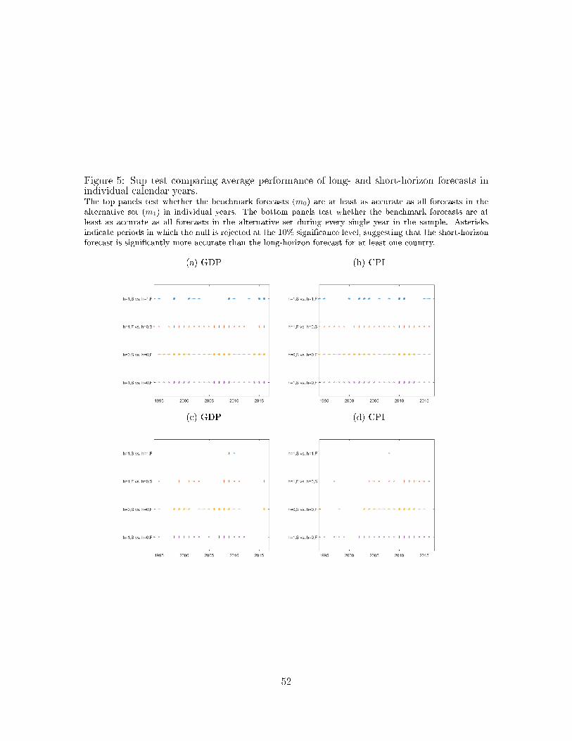
Figure 5: Sup test comparing average performance of long- and short-horizon forecasts inindividual calendar years.The top panels test whether the benchmark forecasts (m0) are at least as accurate as all forecasts in thealternative set (m1) in individual years. The bottom panels test whether the benchmark forecasts are atleast as accurate as all forecasts in the alternative set during every single year in the sample. Asterisksindicate periods in which the null is rejected at the 10% signi�cance level, suggesting that the short-horizonforecast is signi�cantly more accurate than the long-horizon forecast for at least one country.
(a) GDP (b) CPI
(c) GDP (d) CPI
52

Web Appendices
A Monte Carlo Simulations
To explore the �nite-sample performance of our bootstrap procedure for identifying superior
forecasting skills, this section conducts a series of Monte Carlo simulations addressing both
the size and the power of our bootstrap. Consider the following setup: for forecasters
m = 1, ....,M , variables i = 1, ...., N and time periods t + h = 1, ..., T , the forecast errors
are assumed obey the factor structure
ei,t+h,m = λi,mft+h + ui,t+h,m,
where ft+h is a mean-zero Gaussian AR(1) process with autoregressive coe�cient ρ and
variance σ2f . We generate λi,m as i.i.d random variables from a N(0, σ2
λ) distribution trun-
cated such that λ2i,mσ
2f ≤ 0.9; we then set ui,t+h,m as a mean-zero Gaussian AR(1) process
with AR coe�cient ρ and variance 1 − λ2i,mσ
2f . Here, {ft+h}Tt+h=1, {λi,m}1≤i≤N,1≤m≤M
and {ui,t+h,m}1≤i≤N,1≤m≤M,1≤t+h≤T are mutually independent. We set (σf , σλ) = (2, 1.2).
When T > 30, we use ρ = 0.5 and a block size BT = T 0.6; otherwise, we use ρ = 0 and
BT = 1. We consider both a no normalization and a partial normalization scheme, both
of which are described in Example 3.1. Under these schemes, all forecast errors have MSE
values equal to one and thus the null hypothesis that no forecasts underperform the baseline
model, m0, holds.
Table A1 reports size results from 1,200 Monte Carlo simulations using a variety of
combinations for the sample size, T = {25, 50, 100, 200}, the number of forecasters, M =
{2, 10, 100} and the number of outcome variables N = {1, 10, 25, 50, 100}.33 We report
results both with and without studentizing the Sup test statistic and use critical values of
α = 0.05, 0.10.
In general, the size of the non-studentized test statistic is closely aligned with the true
size although it tends to be undersized for large values of N and T , particularly when M is
also large. The size properties of the studentized test statistic are quite good for small-to-
modest values of N,M , and T , but this test statistic tends to be severely undersized when
N,T,M are large. The undersizing is particularly pronounced for α = 0.05. Interestingly,
when the time-series dimension is small (T = 25), the studentized test statistic is actually
over-sized and the rejection rate increases in the number of variables, N . This pattern
reverses in the tests that use larger sample sizes, i.e., T = 50, 100, 200.
The size simulations can be used to compute size-adjusted critical values that deliver
more accurate �nite-sample performance. Although using α as the critical value for the
33Each MC simulation uses 250 bootstraps.
53
p-value leads to asymptotically exact tests, this might not be the case in �nite samples. In
particular, for each value of (N,M, T ), we can compute size-adjusted critical values for the
p-value such that the rejection probability for this sample size under the null hypothesis
is made to be exactly α. Note that whenever the rejection rate in Table A1 exceeds α,
the corresponding size-adjusted p-value, displayed in Table A2, will be adjusted downwards
(below α), whereas the reverse holds when the rejection rate in Table A1 falls below α.
An interesting observation from Table A2 is that using a critical level of α = 0.10 for the
studentized test statistic in many cases gets us close to a size of 5%. This is the chief reason
why we use a 10% size throughout the empirical analysis.
To explore the power properties of the Sup test statistics with and without studentization,
consider the following setup. For each of the N outcome variables, we use one forecast as
the benchmark while the remaining (M − 1) forecasts are competitors. In other words,
we split the NM forecasts into N benchmarks and (N − 1)M competing forecasts. Next,
we randomly select 20% of these competing forecasts and add(2T−1 log(MN)
)1/8to the
selected forecast errors, which then have larger MSE than the baseline forecasts.
This design for the power experiments is in line with that in Chernozhukov et al. (2018).
In their simulations, 5% of the moments violate the null hypothesis while this �gure is
20% in ours. We choose a larger percentage of moments that violate the null hypothesis
due to the smaller sample size in our experiments: their sample size is always 400 and our
sample size ranges from 25 to 200. Because of our smaller sample sizes, it is necessary to
let the magnitude of departures from the null depend on the sample size in order to obtain
meaningful comparisons; if we change(2T−1 log(MN)
)1/8to a �xed value, we would likely
�nd that the methods either have power close to one or close to the nominal size.
Table A3 reports the power of the Sup test statistics with and without studentization.
To facilitate comparisons across the two test statistics, we use size-adjusted critical values.
With exception of a few instances when N = 1, across the board, the power of the Sup test
statistic is much higher with studentization than without, e.g., the power can be 10-20% for
the non-studentized test statistic but 70-80% for the studentized test statistic. The general
conclusion from is, thus, that using the studentized rather than the non-studentized test
statistic yields far better power.
B Proofs
This appendix provides proofs for the theoretical results in our paper.
54

B.1 Preliminary results
Before proving our theorem, we start by recalling some results from Chernozhukov et al.
(2018), re-stated here using our notation so that these results can be readily used in our
analysis. Let qT > rT with qT + rT ≤ T/2. Further, let BT = qT + rT and K = KT =
bT/(qT + rT )c (the integer part of T/(qT + rT )). For 1 ≤ k ≤ K, de�ne Ak = {t : (k −1)(qT + rT ) + 1 ≤ t ≤ (k− 1)(qT + rT ) + qT }. Let {εk}Kk=1 be i.i.d N(0, 1) random variables
that are independent of the data. In the proofs, we use Wt instead of Wt+h for notational
simplicity; changing t+ h to t does not a�ect the theoretical arguments.
Theorem B.1 (Theorem B.1 of Chernozhukov et al. (2018)). Let Assumption 1 hold. Then
there exist constants C, c > 0 depending only on c1, c2 and C1 such that
E supx∈R
∣∣∣∣∣P(
max1≤j≤N
T−1/2T∑t=1
Wjt ≤ x
)
− P
max1≤j≤N
1√KqT
K∑k=1
∑t∈Ak
(Wj,t − µj)εk ≤ x | {Ws}Ts=1
∣∣∣∣∣ ≤ CT−c,where µj = T−1
∑Tt=1Wjt. Moreover,
supx∈R
∣∣∣∣∣P(
max1≤j≤N
T−1/2T∑t=1
Wjt ≤ x
)− P
(max
1≤j≤NZj ≤ x
)∣∣∣∣∣ ≤ CT−c,where Z = (Z1, ..., ZN )′ ∈ RN is a centered Gaussian vector with variance matrix EZZ ′ =
(KqT )−1∑K
k=1E
[(∑t∈AkWt
)(∑t∈AkWt
)′].
Proof. The �rst claim follows from the statement of Theorem B.1 of Chernozhukov et al.
(2018). The second statement is from the proof of Theorem B.1 of Chernozhukov et al.
(2018); see Equation (94) therein.
B.1.1 Bootstrap approximation of normalized test statistic
The following theorem is a general result on the bootstrap approximation of the normalized
test statistic, assuming a good approximation of the normalization. In Appendix B.1.2,
we provide further results on the approximation of the normalization. We �rst state the
following Theorem B.2, present its proof, and then prove the auxiliary lemmas used.
Theorem B.2. Let Assumption 1 hold. Suppose that T−1√KrT (logN )3/2 = o(1),
T−1qT (logN )3/2 = o(1), T−1KrT log2N = o(1) and T−1r2TD
2T log3N = o(1). Let
55

a = (a1, ..., aN )′ ∈ RN be nonrandom with κ1 ≤ aj ≤ κ2 for all 1 ≤ j ≤ N and κ1, κ2 > 0.
Suppose that a = (a1, ..., aN ) satis�es min1≤j≤N aj > 0 and ‖a−a‖∞ = oP (1/ logN ). Then
supx∈R
∣∣∣∣∣P(
max1≤j≤N
T−1/2∑T
t=1Wjt
aj≤ x
)
− P
(max
1≤j≤N
T−1/2∑K
k=1
∑t∈Ak(Wj,t − µj)εkaj
≤ x | {Ws}Ts=1
)∣∣∣∣∣ = oP (1),
where Ak = {t : (k − 1)(qT + rT ) + 1 ≤ t ≤ k(qT + rT )}.
Proof. We �rst apply Theorem B.1 to {(a−11 W1t, ..., a
−1N WN t)}Tt=1, obtaining
E supx∈R
∣∣∣∣∣P(
max1≤j≤N
a−1j T−1/2
T∑t=1
Wjt ≤ x
)
− P
max1≤j≤N
a−1j (KqT )−1/2
K∑k=1
∑t∈Ak
(Wj,t − µj)εk ≤ x | {Ws}Ts=1
∣∣∣∣∣ ≤ CT−c,where C, c > 0 are constants that only depend on c1, c2, C1, κ1 and κ2. By Lemma B.5,
supx∈R
∣∣∣∣∣P max
1≤j≤Na−1j (KqT )−1/2
K∑k=1
∑t∈Ak
(Wj,t − µj)εk ≤ x | {Ws}Ts=1
− P
max1≤j≤N
a−1j T−1/2
K∑k=1
∑t∈Ak
(Wj,t − µj)εk ≤ x | {Ws}Ts=1
∣∣∣∣∣ = oP (1).
Therefore, we have
supx∈R
∣∣∣∣∣P(
max1≤j≤N
a−1j T−1/2
T∑t=1
Wjt ≤ x
)
− P
max1≤j≤N
a−1j T−1/2
K∑k=1
∑t∈Ak
(Wj,t − µj)εk ≤ x | {Ws}Ts=1
∣∣∣∣∣ = oP (1).
It follows from Lemma B.3 that
supx∈R
∣∣∣∣∣P(
max1≤j≤N
a−1j T−1/2
T∑t=1
Wjt ≤ x
)
− P
(max
1≤j≤Na−1j T−1/2
T∑t=1
Wjt ≤ x
)∣∣∣∣∣ = oP (1).
56

The desired result follows from this.
Lemma B.1. Let R = (R1, ..., RN )′, R = (R1, ..., RN )′, ζ = (ζ1, ..., ζN )′, ζ = (ζ1, ..., ζN )′
and Z = (Z1, ..., ZN )′ be random vectors in RN . Suppose that ζ and ζ are F-measurable for some σ-algebra F . Also assume that Z is a centered Gaussian vector with
min1≤j≤N E(Z2j ) ≥ b almost surely for some constant b > 0. If max1≤j≤N |Rj − Rj | =
oP (1/√
logN ) as N →∞ (or other dimensions tend to in�nity), then the following holds:
E supx∈R
∣∣∣∣P ( max1≤j≤N
Zj ≤ x)− P ( max
1≤j≤NRj ≤ x | F)
∣∣∣∣≤ 3E sup
x∈R
∣∣∣∣P ( max1≤j≤N
Zj ≤ x)− P
(max
1≤j≤NRj ≤ x | F
)∣∣∣∣+ o(1).
Moreover, if ‖ζ − ζ‖∞ = oP (1/√
logN ), the following holds:
supx∈R
∣∣∣∣P ( max1≤j≤N
Zj ≤ x)− P
(max
1≤j≤Nζj ≤ x
)∣∣∣∣≤ 3 sup
x∈R
∣∣∣∣P ( max1≤j≤N
Zj ≤ x)− P
(max
1≤j≤Nζj ≤ x
)∣∣∣∣+ o(1).
Proof. Step 1: show the �rst claim.
For an arbitrary η > 0, let c = η/√
logN . De�ne the event M = {max1≤j≤N |Rj −Rj | ≤ c} and variables ξ = max1≤j≤N Rj and ξ = max1≤j≤N Rj . Let aN =
supx∈R |P (max1≤j≤N Zj ≤ x)− P (ξ ≤ x | F)|.We �rst notice that, given the eventM, |ξ − ξ| ≤ c, and thus∣∣∣1 {ξ ≤ x} − 1
{ξ ≤ x
}∣∣∣= 1
{ξ ≤ x and ξ > x
}+ 1
{ξ > x and ξ ≤ x
}= 1
{ξ − ξ ≥ ξ − x and ξ − x > 0
}+ 1
{ξ − ξ < ξ − x and ξ − x ≤ 0
}≤ 1
{|ξ − x| ≤ |ξ − ξ|
}≤ 1 {|ξ − x| ≤ c} . (27)
Hence,∣∣∣P (ξ ≤ x | F)− P (ξ ≤ x | F)∣∣∣
≤ E[∣∣∣1 {ξ ≤ x} − 1
{ξ ≤ x
}∣∣∣ | F]≤ P (|ξ − x| ≤ c | F) + P (Mc | F)
≤ P (ξ ≤ x+ c | F)− P (ξ ≤ x− 2c) + P (Mc | F)
57

≤ P(
max1≤j≤N
Zj ≤ x+ c | F)− P
(max
1≤j≤NZj ≤ x− 2c
)+ P (Mc | F) + 2aN . (28)
Let ι = (1, ..., 1)′ ∈ RN . Then, by Lemma A.1 of Chernozhukov et al. (2017), it follows
that almost surely, for any x ∈ R,
P (Z ≤ (x+ c)ι | F)− P (Z ≤ (x− 2c)ι | F) ≤ 3cCb√
logN ,
where Cb > 0 is a constant that only depends on b. Here, Z ≤ (x+ c)ι means Zj ≤ (x+ c)
for all 1 ≤ j ≤ N ; similarly, Z ≤ (x − 2c)ι means that Zj ≤ (x − 2c) for all 1 ≤ j ≤ N .
Hence, for any z ∈ R, P (Z ≤ zι) = P (max1≤j≤N Zj ≤ z). Therefore, the above display
implies that for any x ∈ R,
P
(max
1≤j≤NZj ≤ x+ c | F
)− P
(max
1≤j≤NZj ≤ x− 2c
)≤ 3cCb
√logN . (29)
By (28), we have∣∣∣P (ξ ≤ x | F)− P (ξ ≤ x | F)∣∣∣ ≤ 3cCb
√logN + 2aN + P (Mc | F).
Since the above display holds for any x ∈ R, we have
supx∈R
∣∣∣P (ξ ≤ x | F)− P (ξ ≤ x | F)∣∣∣ ≤ 3cCb
√logN + 2aN + P (Mc | F),
and, thus,
supx∈R
∣∣∣∣P ( max1≤j≤N
Zj ≤ x)− P (ξ ≤ x | F)
∣∣∣∣ ≤ 3aN + 3cCb√
logN + P (Mc | F).
Taking expectations on both sides, we obtain
E supx∈R
∣∣∣∣P ( max1≤j≤N
Zj ≤ x)− P (ξ ≤ x | F)
∣∣∣∣ ≤ 3EaN+3cCb√
logN+P (Mc) = 3EaN+3ηCb+P (Mc).
Since max1≤j≤N |Rj −Rj | = oP (1/√
logN ), P (Mc) = o(1), and so
E supx∈R
∣∣∣∣P ( max1≤j≤N
Zj ≤ x)− P (ξ ≤ x | F)
∣∣∣∣ ≤ 3EaN + 3ηCb + o(1).
Because η > 0 is arbitrary, it follows that
E supx∈R
∣∣∣∣P ( max1≤j≤N
Zj ≤ x)− P (ξ ≤ x | F)
∣∣∣∣ = EaN + o(1).
58

Step 2: show the second claim.
The argument is similar to Step 1, but we include the details for completeness.
Fix an arbitrary η > 0. Let c1 = η/√
logN , ψ = max1≤j≤N ζj and ψ = max1≤j≤N ζj .
De�ne dN = supx∈R |P (ψ ≤ x)− P (max1≤j≤N Zj ≤ x)|. De�ne the event M1 = {‖ζ −ζ‖∞ ≤ c1}. As in (27), we notice that, given the eventM1,∣∣∣1 {ψ ≤ x} − 1
{ψ ≤ x
}∣∣∣ ≤ 1 {|ψ − x| ≤ c1} .
Thus, ∣∣∣P (ψ ≤ x)− P(ψ ≤ x
)∣∣∣≤ P (|ψ − x| ≤ c1) + P (Mc
1)
= P (x− c1 ≤ ψ ≤ x+ c1) + P (Mc1)
≤ P (ψ ≤ x+ c1)− P (ψ ≤ x− 2c1) + P (Mc1)
≤ P(
max1≤j≤N
Zj ≤ x+ c1
)− P
(max
1≤j≤NZj ≤ x− 2c1
)+ 2dN + P (Mc
1)
(i)
≤ 3c1Cb√
logN + 2dN + P (Mc1),
where (i) follows by (29) (with c replaced by c1). Since the above bound holds for any x ∈ R,we have that, given the eventM1,
supx∈R
∣∣∣P (ψ ≤ x)− P(ψ ≤ x
)∣∣∣ ≤ 3c1Cb√
logN + 2dN = 6c1Cbη + 2dN + P (Mc1).
Therefore,
supx∈R
∣∣∣∣P ( max1≤j≤N
Zj ≤ x)− P
(ψ ≤ x
)∣∣∣∣ ≤ 6c1Cbη + 3dN + P (Mc1).
Notice that P (Mc1) = o(1) due to ‖ζ − ζ‖∞ = oP (1/
√logN ). Since η > 0 is arbitrary,
we have
supx∈R
∣∣∣P (ψ ≤ x)− P(ψ ≤ x
)∣∣∣ ≤ 3dN + o(1).
This completes the proof.
Lemma B.2. Suppose that Z = (Z1, ..., ZN )′ is a centered Gaussian vector with
max1≤j≤N E(Z2j ) ≤ b for some constant b > 0. Then for any z ∈ (0,N/5),
P(‖Z‖∞ ≥
√2b log(N/z)
)≤ 2z.
Proof. Clearly, Zj/√EZ2
j ∼ N(0, 1). Thus, P(|Zj |/
√EZ2
j > x)
= 2Φ(−x) = 2 − 2Φ(x),
59

where Φ(·) denotes the cdf of a N(0, 1) variable. Since EZ2j ≤ b, we have that for any x > 0,
P(|Zj | >
√bx)≤ 2(1− Φ(x)). By the union bound, it follows that for any x > 0,
P
(max
1≤j≤N|Zj | >
√bx
)≤ 2N (1− Φ(x)).
Taking x = Φ−1(1 − a) for a ∈ (0, 1), we have P (‖Z‖∞ >√bΦ−1(1 − a)) ≤ 2Na. By
Lemma 1 of Zhu and Bradic (2018), for a ≤ 1/5, Φ−1(1 − a) ≤√
2 log(1/a). This means
that P (‖Z‖∞ >√
2b log(1/a)) ≤ 2Na. The desired result follows by setting a = z/N .
Lemma B.3. Let the assumptions of Theorem B.2 hold. Then
supx∈R
∣∣∣∣∣P(
max1≤j≤N
a−1j T−1/2
T∑t=1
Wjt ≤ x
)
− P
(max
1≤j≤Na−1j T−1/2
T∑t=1
Wjt ≤ x
)∣∣∣∣∣ = oP (1).
Proof. De�ne ζ = (ζ1, ..., ζN )′ and ζ = (ζ1, ..., ζN )′, where ζj = a−1j T−1/2
∑Tt=1Wjt and
ζj = a−1j T−1/2
∑Tt=1Wjt. Also, let Z = (Z1, ..., ZN )′ ∈ RN be a centered Gaussian vector
with variance matrix EZZ ′ = (KqT )−1∑K
k=1E
[(∑t∈AkWt
)(∑t∈AkWt
)′].
By Theorem B.1, we have
supx∈R
∣∣∣∣P ( max1≤j≤N
Zj ≤ x)− P
(max
1≤j≤Nζj ≤ x
)∣∣∣∣ = o(1). (30)
Applying the same argument with (Zj , ζj) replaced by (−Zj ,−ζj), we obtain
supx∈R
∣∣∣∣P ( max1≤j≤N
(−Zj) ≤ x)− P
(max
1≤j≤N(−ζj) ≤ x
)∣∣∣∣ = o(1).
By assumption, max1≤j≤N EZ2j ≤ C1. Hence, by Lemma B.2, we have that, for any
η ∈ (0, 1/5),
P(‖Z‖∞ ≥
√2C1 log(ηN )
)≤ 2η.
It follows that
P
(max
1≤j≤Nζj >
√2C1 log(ηN )
)≤ P
(max
1≤j≤NZj >
√2C1 log(ηN )
)+ o(1) ≤ 2η + o(1)
60

and
P
(max
1≤j≤N(−ζj) >
√2C1 log(ηN )
)≤ P
(max
1≤j≤N(−Zj) >
√2C1 log(ηN )
)+o(1) ≤ 2η+o(1).
Therefore,
P(‖ζ‖∞ >
√2C1 log(ηN )
)≤ P
(max
1≤j≤Nζj >
√2C1 log(ηN )
)+ P
(max
1≤j≤N(−ζj) >
√2C1 log(ηN )
)≤ 4η + o(1).
Since η is arbitrary, we have
‖ζ‖∞ = OP
(√logN
). (31)
By Assumption 1, min1≤j≤N E(Z2j ) ≥ c1. Next, we verify
‖ζ − ζ‖∞ = oP (1/√
logN ). (32)
Notice that ζj = a−1j ajζj . Thus,
‖ζ − ζ‖∞ = max1≤j≤N
|ζj − ζj | ≤ ‖ζ‖∞ max1≤j≤N
∣∣∣a−1j aj − 1
∣∣∣ .Since min1≤j≤N aj ≥ κ1 and ‖a − a‖∞ = oP (1), we have max1≤j≤N
∣∣∣a−1j aj − 1
∣∣∣ =
OP (‖a− a‖∞). Since ‖ζ‖∞ = OP (√
logN ), we have (32) by the assumption on ‖a− a‖∞.Therefore, from Lemma B.1, we have
supx∈R
∣∣∣∣P ( max1≤j≤N
Zj ≤ x)− P
(max
1≤j≤Nζj ≤ x
)∣∣∣∣≤ 3 sup
x∈R
∣∣∣∣P ( max1≤j≤N
Zj ≤ x)− P
(max
1≤j≤Nζj ≤ x
)∣∣∣∣+ oP (1)(i)= oP (1),
where (i) follows by (30). Now by the triangular inequality, (30) implies
supx∈R
∣∣∣∣P ( max1≤j≤N
ζj ≤ x)− P
(max
1≤j≤Nζj ≤ x
)∣∣∣∣ = oP (1).
This completes the proof.
61

Lemma B.4. Let the assumptions of Theorem B.2 hold. Then
max1≤j≤N
∣∣∣∣∣∣K∑k=1
∑t∈Ak\Ak
(Wj,t − µj)εk
∣∣∣∣∣∣ = OP
(√KrT logN + rTDT logN + rT
√T−1K logN
),
where Ak = {t : (k − 1)(qT + rT ) + 1 ≤ t ≤ k(qT + rT )} for 1 ≤ k ≤ K − 1 and
AK = {(K − 1)(qT + rT ) + qT + 1, ..., T}.
Proof. For 1 ≤ k ≤ K, let uj,k =∑
t∈Ak\AkWj,tεk. By Berbee's coupling (e.g., Lemma 7.1
of Chen et al. (2016)), there exist variables {vk}Kk=1 with vk = (v1,k, ..., vN ,k)′ such that (1)
{vk}Kk=1 is independent across k and independent of {εk}Kk=1; (2) vk has the same distribution
as∑
t∈Ak\AkWt and (3) P (⋂Kk=1{vk =
∑t∈Ak\AkWt}) ≥ 1−Kβmixing(qT ).
Since εk ∼ N(0, 1), Assumption 1 implies that max1≤j≤N∑K
k=1E(vj,kεk)2 ≤ KrTC1.
Also notice that ‖∑
t∈Ak\AkWt‖∞ ≤ rTDT . It follows by Lemma D.3 of Chernozhukov
et al. (2018) that
E
(max
1≤j≤N
∣∣∣∣∣K∑k=1
vj,kεk
∣∣∣∣∣)≤M
(√KrTC1 logN + rTDT logN
),
where M > 0 is a universal constant. Since max1≤j≤N
∣∣∣∑K−1k=1 vj,kεk
∣∣∣ =
max1≤j≤N |∑K−1
k=1 uj,k| with a probability of at least 1−Kβmixing(qT ) and Kβmixing(qT ) ≤Tβmixing(rT ) = o(1), we have that
max1≤j≤N
∣∣∣∣∣K∑k=1
uj,k
∣∣∣∣∣ = OP
(√KrT logN + rTDT logN
). (33)
In the proof of Lemma B.3, we showed that max1≤j≤N µj = OP (√T−1 logN ); see (31).
By a similar argument, we have max1≤j≤N (−µj) = OP (√T−1 logN ). Hence,
‖µ‖∞ = OP (√T−1 logN ).
It follows that
max1≤j≤N
∣∣∣∣∣∣K∑k=1
∑t∈Ak\Ak
µjεk
∣∣∣∣∣∣ = rT ‖µ‖∞
∣∣∣∣∣K−1∑k=1
εk
∣∣∣∣∣= OP (rT
√T−1 logN ×
√K − 1) = OP (rT
√T−1K logN ).
62

The above display and (33) imply that
max1≤j≤N
∣∣∣∣∣∣K∑k=1
∑t∈Ak\Ak
(Wj,t − µj)εk
∣∣∣∣∣∣ = OP
(√KrT logN + rTDT logN + rT
√T−1K logN
).
This completes the proof.
Lemma B.5. Let the assumptions of Theorem B.2 hold. Then
supx∈R
∣∣∣∣∣P max
1≤j≤Na−1j (KqT )−1/2
K∑k=1
∑t∈Ak
(Wj,t − µj)εk ≤ x | {Ws}Ts=1
− P
max1≤j≤N
a−1j T−1/2
K∑k=1
∑t∈Ak
(Wj,t − µj)εk ≤ x | {Ws}Ts=1
∣∣∣∣∣ = oP (1),
where {Ak}Kk=1 is de�ned in the statement of Lemma B.4.
Proof. De�ne R = (R1, ..., RN )′ and R = (R1, ..., RN )′, where Rj =
a−1j (KqT )−1/2
∑Kk=1
∑t∈Ak(Wj,t − µj)εk and Rj = a−1
j T−1/2∑K
k=1
∑t∈Ak(Wj,t − µj)εk.
Let F denote the σ-algebra generated by {Ws}Ts=1.
Also, let Z = (Z1, ..., ZN )′ ∈ RN be a centered Gaussian vector with variance matrix
EZZ ′ = (KqT )−1∑K
k=1E
[(∑t∈AkWt
)(∑t∈AkWt
)′].
By Theorem B.1, we have
supx∈R
∣∣∣∣P ( max1≤j≤N
Zj ≤ x)− P
(max
1≤j≤NRj ≤ x | F
)∣∣∣∣ = oP (1). (34)
Applying the same argument with (Zj , Rj) replaced by (−Zj ,−Rj), we obtain
supx∈R
∣∣∣∣P ( max1≤j≤N
(−Zj) ≤ x)− P
(max
1≤j≤N(−Rj) ≤ x | F
)∣∣∣∣ = oP (1).
By assumption, max1≤j≤N EZ2j ≤ C1. Hence, by Lemma B.2, we have that, for any
η ∈ (0, 1/5),
P(‖Z‖∞ ≥
√2C1 log(ηN )
)≤ 2η.
It follows that
P
(max
1≤j≤NRj >
√2C1 log(ηN ) | F
)≤ P
(max
1≤j≤NZj >
√2C1 log(ηN )
)+oP (1) ≤ 2η+oP (1)
63

and
P
(max
1≤j≤N(−Rj) >
√2C1 log(ηN ) | F
)≤ P
(max
1≤j≤N(−Zj) >
√2C1 log(ηN )
)+oP (1) ≤ 2η+oP (1).
In turn, we have
P(‖R‖∞ >
√2C1 log(ηN ) | F
)≤ P
(max
1≤j≤NRj >
√2C1 log(ηN ) | F
)+P
(max
1≤j≤N(−Rj) >
√2C1 log(ηN ) | F
)≤ 4η+oP (1).
Since η is arbitrary, we have
‖R‖∞ = OP (√
logN ). (35)
By Assumption 1, min1≤j≤N EZ2j ≥ c1. Hence, by Lemma B.1, it su�ces to verify that
max1≤j≤N
|Rj −Rj | = oP (1/√
logN ). (36)
We notice that
aj√TRj − aj
√KqTRj =
K∑k=1
∑t∈Ak\Ak
(Wj,t − µj)εk.
Hence, by Lemma B.4, we have
max1≤j≤N
∣∣∣aj√TRj − aj√KqTRj∣∣∣ = OP
(√KrT logN + rTDT logN + rT
√T−1K logN
).
Since ‖a− a‖∞ = oP (1) and min1≤j≤N aj ≥ κ1 > 0, we have
max1≤j≤N
∣∣∣Rj − aj a−1j
√KqT /TRj
∣∣∣ = OP
(√T−1KrT logN + T−1/2rTDT logN + rTT
−1√K logN
).
By (35), it follows that
max1≤j≤N
∣∣∣Rj −Rj∣∣∣≤ max
1≤j≤N
∣∣∣Rj − aj a−1j
√KqT /TRj
∣∣∣+ max1≤j≤N
∣∣∣aj a−1j
√KqT /T − 1
∣∣∣× max1≤j≤N
|Rj |
= OP
(√T−1KrT logN + T−1/2rTDT logN + rTT
−1√K logN
)+ max
1≤j≤N
∣∣∣aj a−1j
√KqT /T − 1
∣∣∣OP (√
logN )
64
≤ OP(√
T−1KrT logN + T−1/2rTDT logN + rTT−1√K logN
)+ max
1≤j≤N
∣∣∣aj a−1j − 1
∣∣∣√KqT /TOP (√
logN ) + max1≤j≤N
∣∣∣√KqT /T − 1∣∣∣OP (
√logN ).
(37)
By assumption, we have ‖a− a‖∞ = oP (1/ logN ) and min1≤j≤N aj ≥ κ1 > 0. Observe
that
max1≤j≤N
∣∣∣aj a−1j − 1
∣∣∣√KqT /T ≤ OP ( max1≤j≤N
|aj − aj |)
and∣∣∣√KqT /T − 1∣∣∣ =
1−KqT /T1 +
√KqT /T
<T −KqT
T
<((K + 1)(qT + rT )−KqT )
T=
(K + 1)rT + qTT
.
By the assumptions on the rates in the statement of Theorem B.2, we obtain (36) from
(37). This completes the proof.
We next show the following result.
B.1.2 Preliminary results on variance approximation
Lemma B.6. Let the assumptions of Theorem B.2 hold. Moreover, suppose that βmixing(i) .
exp(−b1ib2). Then
max1≤j≤N
|T−1T∑t=1
(Wj,t − E(Wj,t))| = OP
(DTT
−1/2(
logN + (log T )1/(2b2)))
.
Proof. We apply Bernstein's blocking technique with the same block structure as Ak and
Ak, but the choice of K and qT is only speci�c to the proof of this lemma. Let Rk,j =∑t∈Ak(Wj,t − E(Wj,t)). We choose rT such that Kβmixing(rT ) = o(1). This means that
KqT exp(−b1rb2T ) = o(1).
By Berbee's coupling and Lemma 8 of Chernozhukov et al. (2015), it follows that
max1≤j≤N
∣∣∣∣∣K∑k=1
Rk,j
∣∣∣∣∣= OP
max1≤j≤N , 1≤k≤K
|Rk,j |√
logN +
√√√√ max1≤j≤N
K∑k=1
ER2k,j × logN
65

≤ OP
max1≤k≤K
|Ak| max1≤j≤N , 1≤t≤T
|Wj,t − E(Wj,t)|√
logN +
√√√√ max1≤j≤N
K∑k=1
ER2k,j × logN
(i)= OP
(DT qT
√logN +DT
√KqT logN
),
where (i) follows from the de�nition of Ak and ER2k,j . D2
T qT (due to Lemma 7.2 of Chen
et al. (2016)). Moreover,
max1≤j≤N
∣∣∣∣∣T∑t=1
(Wj,t − E(Wj,t))−K∑k=1
Rk,j
∣∣∣∣∣ = max1≤j≤N
∣∣∣∣∣∣K∑k=1
∑t∈Ak/Ak
(Wj,t − E(Wj,t))
∣∣∣∣∣∣≤ 2DT
K∑k=1
|Ak/Ak| ≤ 2DT (KrT + qT ).
Therefore,
max1≤j≤N
∣∣∣∣∣T∑t=1
(Wj,t − E(Wj,t))
∣∣∣∣∣ = OP
(DT qT
√logN +DT
√KqT logN +DTKrT
).
Using K � T/(qT + rT ), we choose qT �√TrT /
√logN to get
max1≤j≤N
∣∣∣∣∣T∑t=1
(Wj,t − E(Wj,t))
∣∣∣∣∣ = OP
(DT
√T logN +DT
√TrT
).
Now the requirement of KqT exp(−b1rb2T ) = o(1) implies that we can choose rT �(log T )1/b2 , which means that
max1≤j≤N
∣∣∣∣∣T∑t=1
(Wj,t − E(Wj,t))
∣∣∣∣∣ = OP
(DT
√T(
logN + (log T )1/(2b2)))
.
The desired result follows from this.
Lemma B.7. Let the assumptions of Theorem B.2 hold. Moreover, suppose that
Kβmixing(qT + rT ) = o(1). Then
max1≤j≤N
∣∣∣∣∣∣T−1K∑k=1
∑t∈Ak
(Wj,t − µj)
2
− E
∑t∈Ak
(Wj,t − µj)
2∣∣∣∣∣∣= OP
(√T−1(qT + rT )D4
T logN + T−1(qT + rT )2D2T logN
).
66

Proof. For simplicity, we assume that K is an even number and denote LT = K/2. Since
Kβmixing(qT + rT ) = o(1), we can use Berbee's coupling and Lemma 8 of Chernozhukov
et al. (2015), obtaining
max1≤j≤N
∣∣∣∣∣∣LT∑l=1
∑t∈A2l−1
(Wj,t − µj)
2
− E
∑t∈A2l−1
(Wj,t − µj)
2∣∣∣∣∣∣= OP
√√√√√ LT∑
l=1
E
∑t∈A2l−1
(Wj,t − µj)
4
logN + max1≤l≤LT , 1≤j≤N
∑t∈A2l−1
(Wj,t − µj)
2
× logN
(i)= OP
√√√√ LT∑
l=1
|A2l−1|2(2DT )4 × logN + max1≤l≤LT
|A2l−1|2(2DT )2 × logN
= OP
(√T (qT + rT )D4
T logN + (qT + rT )2D2T logN
),
where (i) follows by E(∑
t∈A2l−1(Wj,t − µj)
)4. |A2l−1|2(2DT )4 (due to Lemma 7.2 of Chen
et al. (2016)). Similarly, we can show
max1≤j≤N
∣∣∣∣∣∣LT∑l=1
∑t∈A2l
(Wj,t − µj)
2
− E
∑t∈A2l
(Wj,t − µj)
2∣∣∣∣∣∣= OP
(√T (qT + rT )D4
T logN + (qT + rT )2D2T logN
).
The desired result follows from this.
B.2 Proof of Theorem 3.1
We apply Theorem B.2. We separate KT = qT + rT with qT > rT . Speci�cally, we choose
rT = κ1(log T )1/b2 with κ1 = (2/b1)1/b2 and qT = KT − rT . It su�ces to show that the
conditions of Theorem B.2 can be satis�ed by this choice of (qT , rT ).
Since K � T/(qT + rT ) and (rT /qT ) log2N = o(1), we have T−1√KrT (logN )3/2 = o(1)
and T−1KrT log2N = o(1). By qTDT log5/2(NT ) ≤ C1T1/2−c2 and rT < qT , we have
T−1qT (logN )3/2 = o(1) and T−1r2TD
2T log3N = o(1). It remains to show that Assumption
1 is satis�ed by this choice of (qT , rT ). In particular, with N = N , we need to verify the
following
max{Kβmixing(rT ), (rT /qT ) log2N} ≤ C1T−c2 (38)
67

and
qTDT log5/2(NT ) ≤ C1T1/2−c2 (39)
for some 0 < c2 < 1/4.
Since βmixing(rT ) . exp(−b1rb2T ), K ≤ T , it follows that Kβmixing(rT ) . T exp(−b1rb2T ).
Hence, we have Kβmixing(rT ) . T−1.
Since K � T/(qT + rT ) and qT > rT , we have qT � T/K. Therefore,
(rT /qT ) log2N . (log T )1/b2KT−1 log2N .
By Assumption 1, KT−1 log2N . T−b for some b ∈ (0, 1/4). Thus, we only need to
choose c2 = b/2 to obtain (rT /qT ) log2N . T−c2 . This proves (38).
By qT � T/K and Assumption 1, we have
qTDT log5/2(NT ) � K−1TDT log5/2(NT ) . T 1/2−b . T 1/2−c2 ,
which proves (39). Now we have veri�ed all the conditions of Theorem B.2, which implies
that
supx∈R
∣∣∣∣∣P(
max1≤j≤N
T−1/2∑T
t=1Wjt
aj≤ x
)
− P
(max
1≤j≤N
T−1/2∑K
k=1
∑t∈Ak(Wj,t − µj)εkaj
≤ x | {Ws}Ts=1
)∣∣∣∣∣ = oP (1).
This means that
limT→∞
P
(max
1≤j≤N
T−1/2∑T
t=1(Uj,t − EUj,t)aj
> Q∗T,1−α
)= α.
Under the null hypothesis of EUj,t ≤ 0, we have that
max1≤j≤N
T−1/2∑T
t=1(Uj,t − EUj,t)aj
≥ max1≤j≤N
T−1/2∑T
t=1 Uj,taj
= RT .
In turn, this means that
lim supT→∞
P(RT > Q∗T,1−α
)≤ α.
When EUj,t = 0, the inequality in the above two equation displays hold with equality.
This completes the proof.
68

B.3 Proof of Lemma 3.1
We consider two cases.
Case 1: aj = 1.
We only need to take aj = 1. Then aj − aj = 1 and the result clearly holds.
Case 2: aj =
√K−1
∑Kj=1
(B−1/2T
∑t∈Hj (∆Li,t+h − µi)
)2.
We inherit all the notations from before. Recall µj = T−1∑T
t=1Wj,t. Let a2j =
T−1∑K
k=1E(∑
t∈Ak(Wj,t − µj))2
with µj = T−1∑T
t=1E(Wj,t). Let Wj,t = Wj,t − µj and
a2j = T−1
∑Kk=1
(∑t∈Ak Wj,t
)2. Clearly, µj − µj = T−1
∑Tt=1 Wj,t.
Notice that by triangular inequality for the Euclidean norm in RK , we have
max1≤j≤N
|aj − aj | = T−1/2 max1≤j≤N
∣∣∣∣∣∣∣√√√√√ K∑
k=1
∑t∈Ak
Wj,t − |Ak|(µj − µj)
2
−
√√√√√ K∑k=1
∑t∈Ak
Wj,t
2∣∣∣∣∣∣∣
≤ T−1/2 max1≤j≤N
√√√√ K∑k=1
|Ak|2(µj − µj)2
≤ T−1/2‖µ− µ‖∞ max1≤k≤K
|Ak|√K
(i)= OP
(DTT
−1(
logN + (log T )1/(2b2))× (qT + rT )
√K)
= OP
(DTK
−1/2(
logN + (log T )1/(2b2)))
,
where (i) follows from Lemma B.6. On the other hand, Lemma B.7 implies that
max1≤j≤N
∣∣a2j − a2
j
∣∣ = OP
(√T−1(qT + rT )D4
T logN + T−1(qT + rT )2D2T logN
).
Notice that the rate conditions in the assumption imply that the rate in the above
two displays are oP (1/ logN ). Since min1≤j≤N aj is bounded away from zero, we have
max1≤j≤N |aj − aj | = oP (1/ logN ).
The proof for the other cases follows by similar arguments as for Case 2.
69

Table A1: Finite-sample size of Sup tests computed across multiple variables, forecasters, and time-periods
α = 0.05 α = 0.1Without studentization With studentization Without studentization With studentization
M = 2 M = 2 M = 2 M = 2N \ T 25 50 100 200 25 50 100 200 n \ T 25 50 100 200 25 50 100 200
1 0.063 0.060 0.050 0.057 0.058 0.063 0.049 0.057 1 0.117 0.135 0.111 0.113 0.117 0.131 0.116 0.11710 0.054 0.050 0.049 0.052 0.059 0.047 0.027 0.023 10 0.109 0.112 0.105 0.108 0.126 0.113 0.077 0.08125 0.053 0.048 0.045 0.056 0.073 0.033 0.026 0.014 25 0.115 0.112 0.093 0.112 0.141 0.098 0.076 0.07350 0.039 0.047 0.040 0.048 0.052 0.022 0.022 0.020 50 0.086 0.117 0.097 0.100 0.122 0.087 0.054 0.059100 0.033 0.036 0.040 0.039 0.082 0.027 0.011 0.015 100 0.087 0.099 0.109 0.086 0.148 0.074 0.058 0.045
M = 10 M = 10 M = 10 M = 10N \ T 25 50 100 200 25 50 100 200 n \ T 25 50 100 200 25 50 100 200
1 0.049 0.063 0.059 0.049 0.057 0.044 0.040 0.032 1 0.121 0.158 0.143 0.119 0.113 0.134 0.113 0.08810 0.068 0.053 0.043 0.047 0.077 0.034 0.021 0.021 10 0.134 0.143 0.121 0.104 0.155 0.101 0.075 0.06825 0.057 0.067 0.045 0.041 0.087 0.019 0.009 0.008 25 0.127 0.155 0.123 0.130 0.170 0.083 0.043 0.04950 0.042 0.047 0.056 0.035 0.099 0.020 0.006 0.007 50 0.105 0.135 0.123 0.095 0.196 0.072 0.044 0.033100 0.036 0.033 0.019 0.026 0.121 0.025 0.004 0.003 100 0.104 0.100 0.077 0.070 0.231 0.079 0.030 0.031
M = 100 M = 100 M = 100 M = 100N \ T 25 50 100 200 25 50 100 200 n \ T 25 50 100 200 25 50 100 200
1 0.053 0.072 0.051 0.047 0.075 0.039 0.021 0.020 1 0.150 0.165 0.137 0.128 0.135 0.114 0.084 0.07010 0.059 0.062 0.047 0.036 0.114 0.023 0.005 0.004 10 0.122 0.165 0.131 0.117 0.227 0.098 0.051 0.03625 0.042 0.034 0.042 0.038 0.130 0.020 0.007 0.002 25 0.113 0.120 0.126 0.100 0.283 0.083 0.033 0.02350 0.039 0.030 0.024 0.028 0.179 0.016 0.002 0.002 50 0.102 0.129 0.086 0.086 0.369 0.081 0.025 0.021100 0.031 0.023 0.016 0.022 0.237 0.007 0.001 0.002 100 0.067 0.088 0.070 0.063 0.430 0.063 0.013 0.011
Notes: This table presents the size of Sup tests comparing the �nite-sample accuracy of a set of benchmark forecasts m0 to a set of alternative forecasts, m1. All numbers are basedon 2,000 Monte Carlo simulations conducted under the null of equal predictive accuracy of the forecasts in m0 and m1. N denotes the number of variables; M refers to the number offorecasters, while T denotes the number of time-series observations. The two panels on the left present results set the asymptotic size of the test to α = 0.05 while the two panels onthe right set the asymptotic size of the test to α = 0.10. The Monte Carlo simulations generate the forecast errors as ei,t+h,m = λi,mft+h + ui,t+h,m, where ft is a mean-zero GaussianAR(1) process with autoregressive coe�cient ρ and variance σ2
f . We generate λi,m as i.i.d random variables from a N(0, σ2λ) distribution and truncated such that λ2
i,mσ2f ≤ 0.9; we
then set ui,t+h,m as a mean-zero Gaussian AR(1) process with AR coe�cient ρ and variance 1 − λ2i,mσ
2f . {ft+h}Tt+h=1, {λi,m}1≤i≤n,1≤m≤M and {ui,t+h,m}1≤i≤n,1≤m≤M,1≤t+h≤T are
assumed to be mutually independent. We choose (σf , σλ) = (2, 1.2). When T > 30, we use ρ = 0.5 and a block size of BT = T 0.6; otherwise we use ρ = 0 and BT = 1. We consider twostudentization schemes: no studentization (the �rst and third panels) and (partial) studentization (the second and fourth panel), which are both described in Example 1. Under thisscheme, all forecast errors have an MSE equal to one and thus the null hypothesis that no forecasts underperforms the baseline model holds.
70

Table A2: Size-adjusted critical values for the Sup test
α = 0.05 α = 0.1Without studentization With studentization Without studentization With studentization
M = 2 M = 2 M = 2 M = 2N \ T 25 50 100 200 25 50 100 200 n \ T 25 50 100 200 25 50 100 200
1 0.040 0.048 0.052 0.044 0.048 0.040 0.052 0.044 1 0.084 0.076 0.084 0.088 0.076 0.080 0.080 0.08810 0.048 0.052 0.052 0.048 0.040 0.052 0.080 0.080 10 0.096 0.088 0.096 0.092 0.076 0.092 0.124 0.12025 0.048 0.056 0.056 0.044 0.032 0.064 0.080 0.084 25 0.096 0.092 0.108 0.092 0.068 0.108 0.132 0.12850 0.068 0.056 0.064 0.052 0.048 0.068 0.092 0.092 50 0.112 0.092 0.104 0.104 0.088 0.112 0.140 0.152100 0.064 0.060 0.060 0.072 0.032 0.076 0.092 0.108 100 0.112 0.104 0.096 0.112 0.064 0.124 0.136 0.168
M = 10 M = 10 M = 10 M = 10N \ T 25 50 100 200 25 50 100 200 n \ T 25 50 100 200 25 50 100 200
1 0.052 0.040 0.048 0.052 0.044 0.056 0.056 0.068 1 0.084 0.072 0.076 0.084 0.092 0.080 0.092 0.11210 0.036 0.048 0.056 0.052 0.036 0.068 0.080 0.080 10 0.076 0.080 0.088 0.096 0.060 0.100 0.120 0.12825 0.044 0.040 0.056 0.052 0.024 0.080 0.108 0.104 25 0.088 0.072 0.088 0.088 0.060 0.112 0.148 0.15650 0.056 0.056 0.048 0.064 0.020 0.084 0.108 0.132 50 0.096 0.084 0.088 0.104 0.052 0.116 0.156 0.180100 0.064 0.068 0.076 0.084 0.016 0.076 0.128 0.140 100 0.100 0.104 0.116 0.124 0.040 0.116 0.172 0.188
M = 100 M = 100 M = 100 M = 100N \ T 25 50 100 200 25 50 100 200 n \ T 25 50 100 200 25 50 100 200
1 0.048 0.036 0.048 0.052 0.036 0.060 0.076 0.084 1 0.072 0.064 0.080 0.084 0.076 0.092 0.116 0.12810 0.044 0.044 0.052 0.056 0.024 0.076 0.100 0.120 10 0.088 0.068 0.080 0.092 0.044 0.104 0.140 0.16825 0.056 0.060 0.056 0.064 0.016 0.076 0.112 0.132 25 0.096 0.092 0.084 0.104 0.040 0.112 0.160 0.18450 0.060 0.064 0.072 0.068 0.012 0.084 0.128 0.148 50 0.100 0.088 0.112 0.112 0.028 0.116 0.172 0.196100 0.080 0.076 0.084 0.084 0.008 0.096 0.140 0.176 100 0.128 0.108 0.128 0.132 0.016 0.124 0.176 0.224
Notes: This table presents size-adjusted critical values for Sup tests conducted on �nite sample data generated in a Monte Carlo simulation. Here, N denotes the number of variables;M is the number of forecasters, and T is the number of time periods. The two panels on the left present results when the asymptotic size of the test is set to α = 0.05 while the twopanels on the right present result when the asymptotic size of the test is set to α = 0.10. For each value of (N,M, T ), we compute the critical value for the p-value such that the rejectionprobability for this sample size under the null hypothesis is set to equal α. We refer to these critical values as size-adjusted critical values. We consider two studentization schemes: nostudentization (�rst and third panels) and (partial) studentization (second and fourth panels), both being described in Example 1. The forecast errors are generated in the same wayas those in table A1.
71

Table A3: Power of Sup test using size-adjusted critical values
α = 0.05 α = 0.1Without studentization With studentization Without studentization With studentization
M = 2 M = 2 M = 2 M = 2N \ T 25 50 100 200 25 50 100 200 n \ T 25 50 100 200 25 50 100 200
1 0.050 0.053 0.057 0.035 0.054 0.045 0.064 0.038 1 0.095 0.087 0.105 0.090 0.082 0.083 0.095 0.09310 0.112 0.129 0.169 0.170 0.351 0.378 0.589 0.702 10 0.218 0.240 0.305 0.304 0.462 0.515 0.682 0.77525 0.109 0.131 0.121 0.114 0.461 0.576 0.790 0.903 25 0.216 0.208 0.280 0.255 0.609 0.712 0.892 0.95050 0.140 0.107 0.144 0.124 0.657 0.690 0.884 0.975 50 0.218 0.196 0.225 0.234 0.770 0.834 0.955 0.994100 0.100 0.105 0.100 0.159 0.621 0.771 0.922 0.993 100 0.197 0.205 0.180 0.244 0.776 0.890 0.976 0.999
M = 10 M = 10 M = 10 M = 10N \ T 25 50 100 200 25 50 100 200 n \ T 25 50 100 200 25 50 100 200
1 0.473 0.312 0.444 0.610 0.298 0.299 0.384 0.584 1 0.559 0.468 0.551 0.706 0.415 0.393 0.500 0.68710 0.095 0.112 0.125 0.146 0.637 0.723 0.873 0.978 10 0.182 0.207 0.213 0.274 0.733 0.827 0.945 0.99825 0.092 0.097 0.128 0.135 0.644 0.829 0.963 0.998 25 0.184 0.204 0.212 0.258 0.818 0.905 0.991 1.00050 0.097 0.133 0.117 0.159 0.650 0.816 0.967 1.000 50 0.213 0.241 0.218 0.279 0.829 0.904 0.990 1.000100 0.125 0.150 0.171 0.246 0.645 0.823 0.992 1.000 100 0.241 0.261 0.281 0.365 0.815 0.925 0.999 1.000
M = 100 M = 100 M = 100 M = 100N \ T 25 50 100 200 25 50 100 200 n \ T 25 50 100 200 25 50 100 200
1 0.721 0.508 0.721 0.857 0.560 0.651 0.822 0.932 1 0.824 0.710 0.864 0.938 0.719 0.763 0.909 0.96510 0.091 0.089 0.141 0.162 0.668 0.834 0.951 0.998 10 0.227 0.176 0.229 0.296 0.798 0.907 0.982 1.00025 0.130 0.155 0.144 0.185 0.700 0.843 0.958 0.999 25 0.239 0.252 0.240 0.312 0.843 0.943 0.995 1.00050 0.158 0.165 0.172 0.186 0.702 0.871 0.986 1.000 50 0.246 0.235 0.319 0.351 0.850 0.928 0.995 1.000100 0.182 0.155 0.208 0.249 0.701 0.935 0.987 1.000 100 0.319 0.285 0.372 0.443 0.812 0.979 0.998 1.000
Notes: This table reports the �nite-sample power of the Sup test conducted across multiple variables, forecasters and time-periods. N denotes the number of variables; M is thenumber of forecasters and T is the number of time periods. The two panels on the left present results using the 5% size-adjusted critical values from Table A2; the two panels on the rightpresent result using the 10% size-adjusted critical values from Table A2. We consider two studentization schemes: no studentization (�rst and third panels) and (partial) studentization(second and fourth panels), which are both described in Example 1. To investigate the power properties, we consider the following. Of all the Mn forecasts, N forecasts are assignedto the baseline set m0 (i.e., each of the N series has one baseline forecasts) while (N − 1)M forecasts are assigned to the set of alternatives, m1. All forecast errors are generated in thesame way as the simulation described in Table A1. Then, we randomly select 20% of the competing forecasts and add (2T−1 log(Mn))1/8 to their selected forecast errors, which thenhave larger MSE values than the baseline forecasts.
72