MEMORANDUM

No 37/2003

Rolf Aaberge, Ugo Colombino and Steinar

Strøm

ISSN: 0801-1117

Department of Economics University of Oslo

Do More Equal Slices Shrink the Cake? An Empirical Investigation of Tax-Transfer Reform

Proposals in Italy

This series is published by the University of Oslo Department of Economics

In co-operation with The Frisch Centre for Economic Research

P. O.Box 1095 Blindern N-0317 OSLO Norway Telephone: + 47 22855127 Fax: + 47 22855035 Internet: http://www.oekonomi.uio.no/ e-mail: econdep@econ.uio.no

Gaustadalleén 21 N-0371 OSLO Norway Telephone: +47 22 95 88 20 Fax: +47 22 95 88 25 Internet: http://www.frisch.uio.no/ e-mail: frisch@frisch.uio.no

List of the last 10 Memoranda: No 36 Kari Eika

Low Quality-Effective Demand. 43 pp. No 35 Karl Ove Moene

Social Democracy as a Development Strategy. 35 pp. No 34 Finn Roar Aune, Rolf Golombek and Sverre A. C. Kittelsen

Does Increased Extraction of Natural Gas Reduce Carbon Emissions?. 40 pp.

No 33 Christoph Schwierz The Effects of Taxes and Socioeconomic Variables on Market Work and Home Production in Norway in the Years 1970 to 2000. 61 pp.

No 32 John K. Dagsvik, Steinar Strøm and Zhiyang Jia A Stochastic Model for the Utility of Income. 39 pp.

No 31 Karine Nyborg, Richard B. Howarth, and Kjell Arne Brekke Green consumers and public policy: On socially contingent moral motivation. 25 pp.

No 30 Halvor mehlum A Finer Point in Forensic Identification. 11 pp.

No 29 Svenn-Erik Mamelund Effects of the Spanish Influenza Pandemic of 1918-19 on Later Life Mortality of Norwegian Cohorts Born About 1900. 30 pp.

No 28 Fedor Iskhakov Quasi-dynamic forward-looking model for joint household retirement decision under AFP scheme. 59 pp.

No 27 Henrik Wiig The Productivity of Social Capital. 22 pp.

A complete list of this memo-series is available in a PDF® format at:

http://www.oekonomi.uio.no/memo/

1

Do More Equal Slices Shrink the Cake?An Empirical Investigation of Tax-Transfer Reform Proposals in Italy

Rolf Aaberge, Research Department, Statistics Norway, Oslo

Ugo Colombino, Department of Economics, University of Turin

Steinar Strøm, Department of Economics, University of Oslo

Abstract

A crucial issue in efficiency-equality evaluations of tax reforms resides in the possibility that the levelas well as the distribution of welfare may change, where the household-specific measures of welfarecapture the value of income as well as the value of leisure. A better-designed redistribution andincome support system may not only foster equality but also improve the configuration of incentivesand by this route contribute in its turn to efficiency. This paper presents an empirical analysis of thewelfare effects for married couples of replacing the Italian tax system by three alternative hypotheticalreforms: a flat tax, a negative income tax, and a work fare scheme. We employ a microeconometricmodel of household labour supply that represents partners’ simultaneous choices, allows forconstraints in the choice of hours of work, and is sufficiently flexible to capture a large variety ofsupply responses. These features appear to be crucial in the evaluation of reform effects. The resultssuggest that there is scope for improving upon the current system under both the efficiency and theequality criterion. The benefits from the reforms, however, come from unexpected directions since thelargest labour supply contribution to the increase in welfare come from poor and middle classhouseholds whereas rich households appear to be much less responsive to changes in the tax rates.The simulation results reveal that a crucial role in shaping the results is played by the relatively higherbehavioural responsiveness of married women living in low and average income households.

Keywords: Tax reforms, labour supply, welfare gains and losses, efficiency-equality trade-off, socialwelfare

JEL classification: D19, D69, J22

2

1. IntroductionIn the last few years a debate has developed in Italy upon reforming the tax-transfer treatment of

households. Although with some delay, the debate follows closely enough policy discussions that are

going on in other OECD countries, and moves around two focal issues. The first one concerns the

possibly large loss in efficiency due to disincentives and distortions on worker behaviour caused by

progressive taxation. The reform proposals that are mainly motivated by such arguments tend to

suggest a flatter profile of the marginal tax rates (with the pure “flat tax” as a limit case) together with

a reduction of the levels of the tax rates. The second issue stems from the widespread observation that

the current Italian system of transfers and benefits directly or indirectly related to supporting the life

standard of needy or poor or in any sense disadvantaged households performs rather poorly both in

terms of cost-effectiveness and fairness. The reform proposals that are mainly inspired by this

concern by and large converge in supporting some more or less universal basic transfer, or basic

guaranteed level of income, or basic endowment.

The picture is mirrored into the political platforms of alternative coalitions. Since the

publication of a “Libro Bianco” on behalf of the Ministry of Finance in 19941, up to the tax reform

proposals contained in the 2001 election platform, the quest for lower and “flatter” tax rates has been

supported with more energy by the centre-right coalition (“Casa delle Liberta”), while the concern for

a more equitable and cost-effective system of income support and redistribution has been more a

policy focus of the recent centre-left governments2 (“Ulivo”) as well as of the electoral platform of the

centre-left coalition. It must be recognised however that the two issues are more complementary than

alternative. For example, a non-technical article by Rizzi and Rossi (1997) proposes an overall reform

of the tax-transfer system combining a basic universal transfer with a flat tax, very much in line with

the arguments developed in Atkinson (1995). A similar proposal, under the label of “Social

Dividend”, was included in the 2001 electoral platform of the centre-left coalition3.

Previous exercises applied to Italy have adopted non-behavioural simulations for evaluating reforms

similar to the ones mentioned above4. When account is not taken of behavioural responses, the

1 Ministero delle Finanze (1994)2 See Commissione Onofri (1997) for analyses and proposals elaborated upon these issues during the last centre-leftgovernment.3 Ministero del Tesoro (2000).4 Baldini and Bosi (2001) use a static micro-simulation model to evaluate the effects on income distribution and on net taxrevenue of the two reforms contained in the electoral platforms of the two opposed coalitions, and conclude that they both areundesirable. The (almost) flat tax proposal - proposed by the centre-right coalition - would according to the results of Baldiniand Bosi - entail a major loss in revenue; to keep revenue constant an unbearably high rate would be required. On the otherhand, the “social dividend + flat rate” reform - proposed by the centre-left coalition - would have positive effects onredistribution but again would require an exceedingly high flat rate to keep the revenue constant. Another example of non-behavioural simulation analysis of this type of reforms is provided by Bourguignon et al. (1997).

3

dimension of the (gross) “cake” is obviously fixed. However, the crucial issue in efficiency-equality

evaluation resides precisely in the possibility that the dimension (along with the distribution) of the

cake may change. Less distortionary tax rates may generate a larger amount of resources available for

redistribution; a better designed redistribution and income support system may not only foster equality

but also improve the configuration of incentives and by this route contribute in its turn to efficiency.

In this paper we use a model of household labour supply to evaluate stylised versions of the above

reform ideas. A behavioural model might reveal the possibility of improving both efficiency and

equality. We use a pre-estimated household labour supply model, briefly described in Appendix A.

The social evaluation methodology we use is a generalisation of King (1983), where

measures of welfare are derived from equivalent incomes defined in terms of a reference household

and of the prices (wages) and opportunities that this household faces. The introduction of a reference

state (household characteristics, market opportunities and prices) is made in order to compare welfare

across households and opportunity sets5. A recent example of a policy simulation exercise using a

consistent social evaluation methodology that is close to the one adopted in this paper is provided by

Fortin et al. (1993). Their study, however, relies on a calibrated (not estimated) and a rather restrictive

model of household labour supply based on a Stone-Geary utility function that has not been subjected

to empirical testing.

The methodology for welfare evaluation is explained in section 2, whilst the tax reforms in

question and a brief outline of the 1993 tax regime are described in section 3 and Appendix B. The

simulation results are also reported in section 3. Section 4 provides concluding remarks.

2. Behavioural micro-simulation and welfare evaluation The simulation tool is a microeconometric model of household labour supply, previously estimated on

1993 data. Some essential features of the model are synthetically illustrated in Appendix A6. Here we

recall the general format of the estimation and policy simulation steps. The i-th household (a couple)

is assumed to choose a “job” from a choice-set iΩ . The choice set specification accounts for quantity

constraints, limits to the choice of work hours and different opportunities between households and

5 We also checked the sensitivity of the results with respect to the choice of the reference state.6 A full presentation of the model and more details on data and estimation can be found in Aaberge, Colombino and Strøm(1999) and Aaberge, Colombino, Strøm and Wennemo (2000). Some key features are illustrated in Appendix A. The modelallows for observed as well as unobserved characteristics in preferences and opportunities, for spouses’ simultaneousdecisions, for non-convex budget sets due to the complexity of the tax system and for quantity constraints on the choice ofhours of work. Previous structural labour supply models estimated on Italian data include Colombino (1985) and Colombinoand Del Boca (1990).

4

genders. Each job alternative contains wife’s gross wage rate iFw , husband’s wage rate iMw , wife’s

hours of work iFh , husband’s hours of work iFh and other unobserved (by the analysts) characteristics

j. As examples of j we can think of commuting time, environmental characteristics of the job, skill

content of the job etc. The choice set contains also non-market activities, i.e. jobs with 0w = and

0h = . Let i iF iF iM iM iY w h w h m= + + be the gross household income associated with a particular job,

where im represent other (exogenous) income. Net household income under tax-transfer regime k will

then be ( , , )k ki i iF iF iM iM iC Y R w h w h m= − , where ( )kR ⋅ - a function of gross incomes - represents the

tax-transfer rule that computes the net tax to be paid under tax-transfer regime k. Preferences are

represented by the utility function ( , , , )ki i iF iMU C h h j . The i-th household then solves the problem

( , , , )max ( , , , )

. .( , , )

ki iF iM i

ki i iF iM

C h h j

k ki i iF iF iM iM i

U C h h j

s tC Y R w h w h m

∈Ω

= −(2.1)

The observed 1993 behaviour is assumed to be generated by the solution of the problem above under

the 1993 tax-transfer regime. The data set used includes 2160 married couples in age 18-54 belonging

to the 1993 Bank-of-Italy Survey of Household Income and Wealth (SHIW93). On the basis of

observed behaviour we estimate the utility function and the parameters of the choice sets7. The

simulation consists in solving

( )

( , , , )

1993

max ( , , , )

. .( , , )

, , =

ki iF iM i

ki i iF iM

C h h j

k ki i i iF iF iM iM i

ki iF iF iM iM i i

i i

U C h h j

s tC Y R w h w h m

R w h w h m R

∈Ω

= −

∑ ∑

(2.2)

The first constraint is the i-th household's budget constraint. The second one is the constant-tax-

revenue constraint and concerns all households.

7 The estimates of this specific version of the model are presented in Aaberge, Colombino, Strøm and Wennemo (2000).

5

Let ( ), , ki i iV m RΩ represent the maximum utility level attained by household i, endowed

with exogenous income im , facing choice set iΩ and tax-transfer rule kR . Let us consider now a

reference household S that faces choice set SΩ , and a reference tax-transfer rule SR . We ask what is

the exogenous income kiy that would allow the reference household in the reference setting to reach

utility ( ), ; ki i i iV m RΩ :

( ) ( ), , , ,k k Si i i S S iV m R V y RΩ = Ω . (2.3)

Thus, ( ), , ; ,k k k Si i i i Sy y R m R= Ω Ω is a generalisation of the concept of indirect money-metric utility

as defined in Varian (1992) or in King (1983) – where it is called equivalent income8. The use of a

reference choice set SΩ and a reference tax-transfer rule SR allows comparisons between policy

reforms defined by changes in R and/or Ω . The use of a reference household (or reference

household characteristics) makes it meaningful to compare and aggregate the household-specific

equivalent incomes.

Let us suppose the status quo is some tax-transfer rule 0R . Under this regime, household i

attains utility level ( )0, ,i i iV m RΩ . The money-metric representation 0iy of this utility level is

implicitly defined by

( ) ( )0 0, , , , Si i i S S iV m R V y RΩ = Ω (2.4)

Now, a new tax-transfer rule 1R is introduced. The corresponding equivalent income 1iy is defined by

( ) ( )1 1, , , , Si i i i S S iV m R V y RΩ = Ω (2.5)

The equivalent incomes 1iy and 0

iy for household i represent the levels of (exogenous) income that

affords the reference household S the same level of utility under the reference choice set SΩ and the

reference tax-transfer system SR as household i attains under tax systems 1R and 0R (and choice set

8 The concept must not be confused with the homonymous one used in the equivalence scales literature.

6

iΩ ). Thus, the difference between 1iy and 0

iy for household i emerges as an appropriate measure of

the household-specific welfare effect of changing tax-transfer system from 0R to 1R . Moreover,

since the money values of the household's utilities are defined in terms of a reference household who

faces fixed prices and a fixed choice set, this welfare measure are comparable across households. The

difference between the two equivalent incomes can be interpreted as a monetary measure of welfare

change and we will call it Comparable Welfare Gain:

1 0i i iCWG y y= − (2.6)

We use flat tax (FT) as the reference tax system. The reason for this choice is that the

evaluation of the equivalent income defined by equation (2.3) is computationally much more

convenient if the reference system is a system where tax rates are not subject to choice. Any

alternative reference tax system will imply endogenous tax rates. The reference tax-transfer rule will

be the FT rule (defined above) that generates the same net revenue as the actual 1993 rule.

It should be emphasised that due to the random utilities employed here we have to perform

stochastic simulations in order to generate the distribution of the CWGs. The decile-specific mean

values of CWG are reported in section 3.

As indicated above the CWG-values may depend on the choice of reference household.

Thus, it is important to examine the sensitivity of the results with regard to the choice of reference

household. In the simulation exercise that follows, we have alternatively used - as reference - the

household (and the corresponding choice set) with the lowest, the median and the highest observed

income. The results, however, are very similar; therefore, to simplify the exposition, we only report

the results obtained when using the median income household as reference.

Although the distributions of CWG generated by alternative tax reforms provide important

information for evaluating the welfare effects of tax reforms, a complete ranking of these distributions

may require the use of a social welfare function. Moreover, social welfare functions serve as primary

quantities for summarising the information content of the distribution of CWGs. In this study we use

the following family of rank-dependent social welfare functions1

1,

0

( ) ( ) , 1,2,...,b k b kW p t F t dt b−= =∫ (2.7)

where 1kF − is the left inverse of the cumulative distribution function of equivalent income under tax-

transfer rule k and pb(t) is a weight function defined by

7

( )1

log , 1( )

2,3,...1 ,1b b

t bp t b btb

−

− == =− −

(2.8)

where b is the inequality aversion parameter9. Note that the inequality aversion decreases when b

increases. It follows by straightforward calculations that ,b k kW µ≤ = mean of the distribution ( )kF y ,

and that ,b kW is equal to µk if and only if Fk is the egalitarian distribution. Thus, ,b kW can be

interpreted as the equally distributed equivalent level of equivalent income under tax regime k.

Aaberge (2000) demonstrated that the following family of inequality measures,

,, 1 , 1, 2,...b k

b kk

WC b

µ= − = (2.9)

yields a complete characterisation of the distribution function Fk provided that the mean is known10.

Moreover, Aaberge (2000) justified that the use of a few of these inequality measures may give a good

summarisation of inequality in the distribution function.

When the tax-benefit rule is changed from 0R to 1R expression (2.9) can be exploited to

measure the proportionate social gain11 defined by the expression

( )( )

1 ,1,1

,0 0 ,0

11

bbb

b b

CWW C

µξ

µ−

= =−

. (2.10)

Expression (2.10) shows that the effect on social welfare can be decomposed into the product of the

efficiency effect 1

0

µµ

and the equality effect ( )( )

,1

,0

11

b

b

CC

−−

. In the limiting case when b → ∞, ξb reduces

to the ratio between the means of the post- and pre-reform equivalent incomes. Therefore we also

have:

9 Several other authors have discussed rationales for this approach, see e.g. Donaldson and Weymark (1980, 1983), Weymark(1981), Yaari (1988), Ben Porath and Gilboa (1992) and Aaberge (2001).10 Note that

,, 2

b kC b ≥ is the “generalised” Gini family introduced by Mehran (1976). It can be easily verified that C2k is

equal to the Gini coefficient. For unimodal distributions that are not strongly skew to the right or left the Gini coefficient ismost sensitive to changes that take place in the middle part of the income distribution. As noted by Aaberge (2000) C1kexhibits strong downside inequality aversion and is equivalent to a measure of inequality that was introduced by Bonferroni(1930). By contrast, C3k exhibits upside inequality aversion and therefore yields a supplement to the information provided bythe Gini coefficient and the Bonferroni coefficient.

11 The terminology is taken from King (1983).

8

( )( )

,1

,0

11

bb

b

CC

ξ ξ ∞

−=

−(2.11)

3. Tax reformsSince the model we use for the tax simulations is estimated on 1993 data, we take the 1993 tax rule as

the status quo (R0). It is essentially a system of increasing marginal tax rates, going from 10 per cent

(up to 7,2 millions of ITL) to 50 per cent (over 300 millions of ITL), which are applied to individual

total annual income. For more details we refer to the Appendix B. since 1993 the number of brackets

has been reduced, but the essential characteristics of the system are still the same12.

The hypothetical reforms are stylised representations of ideas that – as mentioned in section

1 – are a matter of debate and proposal in Italy as well as in other OECD countries, with differing

focus on different aspects of the tax regime. On the one hand there is a quest for a flatter profile of the

marginal tax rates in order to reduce disincentives and enhance efficiency13. On the other hand, and

specifically in Italy, it is recognised that the system of basic income support provides transfers that are

not cost-effective and do not respond to any explicit design of social or family policy, and that

therefore the system needs to be rationalised on a more transparent and universalistic basis. Under

different labels, the ideas belonging to this second strand, converge on proposing some type of basic

income scheme, either in the form of a universal transfer or in the form of transfer that compensate

incomes up to a basic level. The quests for more efficiency via a flatter tax profile and for more, or

not less, equality via a more cost-effective system of income support are far from being mutually

exclusive. In fact many proposals (e.g. Atkinson, 1995 and, for Italy Rizzi and Rossi, 1997, and more

recently Ministero del Tesoro, 2000) match a flat tax with a basic income scheme. In what follows, we

evaluate three different systems that in one way or another can satisfy these criteria. The first is a

proportional or flat tax (FT). If Y represents total gross income, the tax FTR to be paid by the

household is

FTFTR t Y= (3.1)

12 In the text and in the tables, the figures are in 000's of Italian Lire. In order to translate into EURO, the figures should bedivided by 1.93627.13 Another motivation for less progressive tax rates is to reduce the incentives to evasion and elusion.

9

where FTt is a constant marginal tax rate. Besides incorporating the idea of minimising distortions, it

is also a benchmark system, useful for comparison. As mentioned above it will also be used as the

reference tax rule since it is computationally convenient to do so.

The second reform is a simple negative income tax (NIT), where a flat tax is complemented

with a transfer (a negative tax) that guarantees households’ income up to a basic level G14:

( )NIT

NIT

Y G if Y GR

t Y G if Y G− ≤

= − ≥(3.2)

Last, we consider the so-called WorkFare (WF) system, which essentially is a modification

of NIT where the transfer is received only if the household works a minimum required amount of

hours15,

( )

min

min

0WF

WF

if Y G and H HR Y G if Y G and H H

t Y G if Y G

≤ <= − ≤ > − ≥

(3.3)

where tWF is a constant marginal tax rate, H represent the total hours worked by the wife and the

husband and Hmin is a minimum required number of hours worked (set equal to 1000 in the

simulation). Although similar to the NIT, the WF system is interesting to analyse, both because it may

have better chances to receive political support and because of the theoretical argument according to

which under certain conditions it can be proved to be Pareto-superior to NIT16.

Note that ,FT NITR R and WFR are functions of the wife and husband's earnings and the other

income of the couple. NIT and WF are interpreted as reforms that try to compound the criterion of

lessening distortions from high marginal tax rates and the criterion of redesigning the basic income

14 In this exercise we limit ourselves to the NIT and do not consider the possibly less realistic basic income in the form of auniversal unconditional transfer. The idea of a minimum guaranteed income or alternatively of a universal basic income orwealth transfer, has a long tradition in economics and political philosophy and can be traced back to Tom Paine, CharlesFourier and John Stuart Mill amongst others. More recently, it motivated proposals from scholars with radically differentideology, from Friedman (1964) to Van Parijs (1995), passing through Tobin (1966), Meade (1978) and Atkinson (1995) tocite a few. A recent articulated proposal for a universal transfer in the form of an initial endowment is put forward byAckerman and Alstott (1999). Targetti Lenti (2000) provides a survey with focus on the Italian case.15 In the simulation exercise we put Hmin = 1000 (cumulatively for the two partners). Alternatively - and more generally - onemight think of making the transfer conditional on some other decision made by the household, such as taking part in atraining program.16 See Fortin et al. (1993).

10

support system in a more effective way. Since the actual basic income support policies are thought to

be rather wasteful and occasionally even inequitable, there might be scope for reforms that are able to

increase both efficiency and equality.

For each of the reforms illustrated above, the simulation consists in solving problem (2.2).

For each reform there is a marginal tax rate that must be endogenously determined by the simulation

as the one generating the same total tax revenue as of 1993, given the other parameters of the tax-

transfer rules17. The constant-revenue marginal tax rates turn out to be 0.184 (FT), 0.284 (NIT) and

0.273 (WF). The average net tax rate (i.e. the ratio of total net tax revenue to total gross income) is

0.20 under 1993 regime and goes down to 0.184 (FT), 0.198 (NIT) and 0.195 (WF). Since net tax

revenue is kept constant, the result of a lower average tax rate reveals that all the reforms induce

behavioural changes that generate a larger total gross income18.

As a way of summarising the basic behavioural features implied by the model, before

entering the illustration of reforms simulation, in Table 1 we show the labour supply elasticity with

respect to wage, broken down by gender and household income. They are obtained by increasing gross

wages by 1%, computing the new labour supply choices individual by individual and then averaging

across the sample. We observe a very clear-cut difference of responsiveness between wife and

husband and a marked inverse dependence of elasticity on household income19. This pattern of

elasticities suggests that women living in low or average income households play a crucial role in

determining reform effects, provided the reform implies significant changes in incentives for them.

Table 1 also reveals that cross-elasticities – again mostly for women in low and average income

brackets – are far from irrelevant, thus giving support to the choice of modelling the joint decisions by

household members. Below we suggest that they significantly contribute in explaining some

apparently counterintuitive results.

17 For FT, the marginal tax rate is of course constant for any level of income. For NIT and WF is the (constant) marginal taxrate applied to incomes above the guaranteed level G.18 This effect can be due to more participants, and/or more hours worked among participants, and/or a more productive poolof participants (i.e. a favourable selection effect).19 It is worthwhile noting that the functional form adopted for representing household utility (see Appendix A) does not implya priori any particular relationship between supply elasticity and household income or individual wage.

11

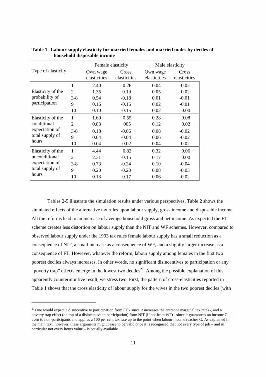
Table 1 Labour supply elasticity for married females and married males by deciles ofhousehold disposable income

Female elasticity Male elasticityType of elasticity Own wage

elasticitiesCross

elasticitiesOwn wageelasticities

Crosselasticities

1 2.40 0.26 0.04 -0.022 1.35 -0.19 0.05 -0.023-8 0.54 -0.18 0.01 -0.019 0.16 -0.16 0.02 -0.01

Elasticity of theprobability ofparticipation

10 0.10 -0.15 0.02 0.001 1.60 0.55 0.28 0.082 0.83 005 0.12 0.023-8 0.18 -0.06 0.08 -0.029 0.04 -0.04 0.06 -0.02

Elasticity of theconditionalexpectation oftotal supply ofhours 10 0.04 -0.02 0.04 -0.02

1 4.44 0.82 0.32 0.062 2.31 -0.15 0.17 0.003-8 0.73 -0.24 0.10 -0.049 0.20 -0.20 0.08 -0.03

Elasticity of theunconditionalexpectation oftotal supply ofhours 10 0.13 -0.17 0.06 -0.02

Tables 2-5 illustrate the simulation results under various perspectives. Table 2 shows the

simulated effects of the alternative tax rules upon labour supply, gross income and disposable income.

All the reforms lead to an increase of average household gross and net income. As expected the FT

scheme creates less distortion on labour supply than the NIT and WF schemes. However, compared to

observed labour supply under the 1993 tax rules female labour supply has a small reduction as a

consequence of NIT, a small increase as a consequence of WF, and a slightly larger increase as a

consequence of FT. However, whatever the reform, labour supply among females in the first two

poorest deciles always increases. In other words, no significant disincentives to participation or any

“poverty trap” effects emerge in the lowest two deciles20. Among the possible explanation of this

apparently counterintuitive result, we stress two. First, the pattern of cross-elasticities reported in

Table 1 shows that the cross elasticity of labour supply for the wives in the two poorest deciles (with

20 One would expect a disincentive to participation from FT - since it increases the entrance marginal tax rate) -, and apoverty trap effect (on top of a disincentive to participation) from NIT (if not from WF) - since it guarantees an income Geven to non-participants and applies a 100 per cent tax rate up to the point when labour income reaches G. As explained inthe main text, however, these arguments might cease to be valid once it is recognised that not every type of job – and inparticular not every hours value – is equally available.

12

respect to the husband’s wage) is positive (0.82 per cent). Also, for a majority of men, the marginal

wage rate increases as a consequence of any of the reforms, particularly on full-time jobs. Given the

positive cross-elasticity, this leads to an increase in the wife’s labour supply. Second, there is a

possible effect of the interactions of the reforms with the quantity constraints on the hours choice. As

explained in Appendix A, the model accounts for the fact that not every type of job is equally

available to every individual. If, for example, part-time jobs are hard to find, at least for some women,

the relevant comparison is the one between non-participation and full-time jobs. In a sense, the

average net wage rate becomes more relevant than the marginal net wage. Thus, it may well be the

case that a reform implies a higher (compared to the 1993 system) net income on a full-time job. This

effect will encourage participation even if the entrance marginal tax rate is higher (FT) or if unearned

income increases (NIT and WF). Note that a traditional model, where different job type availability is

not taken into account, could not have captured such an effect. Overall, it is worthwhile noting that

the specific features of the microeconometric model employed – partners’ simultaneous choices,

constraints in the choice of hours and ability to capture a large variety of supply responses – turn out

to be crucial in explaining the simulation results.

In Table 3 we present the mean value CWGs of the three reforms outlined above,

disaggregated by 1993 household welfare decile and by “winners” and “losers”. For each reform,

three simulation exercises have been performed, using three different reference households. However,

since the results are similar, for simplicity of exposition we only report the results obtained with the

median income household as reference21. All the reforms are more efficient than the 1993 rule, since

for each reform the overall average CWG is positive. Also the overall proportion of winners is always

positive. However, the distributional effects are very different. It seems clear that FT is disequalising,

since the average CWG is negative for the worst-off fraction of the sample. Also, there is a majority

of losers in the worst-off deciles. On the other hand the results of Table 3 suggest that NIT and WF

might be equalising, since the only decile to loose is the best-off one. Note that the identification of

the proportions of winners and losers solely requires ordinal utility information. Thus, the estimates of

the proportions of winners and losers are independent of the choice of reference state.

21 The results obtained with the three different reference households are reported in a working paper by Aaberge, Colombinoand Strøm (2001) that can be downloaded from CHILD web page (www.child-centre.it).

13

Table 2. Participation rates, annual hours of work, gross income, disposable income and taxesfor married couples under alternative tax regimes by deciles of disposable householdincome under 1993-taxes

Annual hours of work Households, 1000 ITL 1993

Taxregime Decile

Participationrates,

per cent

Givenparticipation

In the totalpopulation

Grossincome

Taxes Disposableincome

M F M F M F

1993-tax rules

123-8910

95.697.598.999.399.4

14.119.943.865.574.4

15711832199121172237

10301209154617311828

15011787197021032225

145 241 67711331361

15221 24372 48187 85135128396

525 2109 89601998334365

1469522263392276515294032

All 98.5 43.7 1972 1590 1943 694 54225 11074 43150

FT

123-8910

95.497.899.099.499.5

19.624.444.764.573.2

17061924204821622267

12641397158517411834

16271882202721502257

247 342 70911241344

22933 31761 54142 89459132888

4219 5845 99611646024452

18714 25917 44181 72999108435

All 98.6 45.0 2036 1623 2008 731 60189 11074 49115

NIT

123-8910

95.2897.1398.6399.2199.49

14.4419.9141.4263.2972.59

15511820199621382252

10561240154017331832

14781768196921212241

152 247 63810971331

16404 26199 49801 86985130581

-1952 2537 95382021832714

1835623662402636676797867

All 98.29 41.87 1976 1589 1942 665 55897 11074 44823

WF

123-8910

95.3297.4598.8299.3199.49

15.1920.2842.2063.5672.96

16211866201821452256

11171285154817381833

15451818199421302244

170 260 65311051338

17655 27280 50669 87455131013

-247 2956 94871956931538

1790224324411826788599476

All 98.45 42.52 2001 1597 1970 679 56742 11074 45668Note to Table 2. The results for WF are new, while the results for 1993, FT and NIT are taken fromAaberge et al. (2000).

14

Table 3. The distribution of CWG by losers and winners, and by deciles of household equivalentincome1) under 1993-taxes when the 1993 tax regime is replaced by various alternativetax regimes

Average CWGin 1000 ITL

Tax-

transfer

rule

Deciles WinnersPer cent of

the totalpopulation

All couples Losers Winners

1 41.5 -122 -5228 70512 43.5 457 -5641 83103-8 52.0 2848 -6029 110589 60.1 6307 -6607 1492610 60.9 7325 -8299 17460

FT

All 51.8 3105 -6121 117031 65.3 3039 -2620 60822 59.2 2208 -2762 56343-8 54.6 1736 -3998 65269 51.4 1573 -5595 840810 46.1 -808 -9719 9726

NIT

All 55.0 1643 -4640 68211 64,8 2750 -2656 57322 59,3 2165 -2773 55403-8 55,4 1835 -3958 65319 52,6 1793 -5551 845910 47,6 -478 -9668 9776

WF

All 55,6 1724 -4594 67901) Equivalent income and CWG are defined using the median income household as reference

In Tables 4 and 5 we extend the analysis to the social welfare effect and its components. We

use ,b kW defined by (2.7) and (2.8) for 1, 2, 3 and b = ∞ The corresponding measures of social

welfare have been calculated for both the pre- and post-reform distributions of equivalent income. The

values of proportionate social gain bξ defined by (2.10) are given in Table 4. All the reforms produce

a positive social gain for any value of the inequality aversion parameter b. As we have noted above,

ξ∞ ignores distributional effects and solely captures the efficiency gains of the reform. In other

words, the last column of Table 4 contains the ratio between the average equivalent income under a

certain reform and the average equivalent income under the 1993 rule. Thus, if we only care about

efficiency we look at the last column and read that social gain is 2.1% under FT, 0.8% under NIT and

1.1% under WF. If we also care about the distribution of equivalent income, and we adopt – say – a

Gini welfare function (i.e. we use (2.7) with b = 2), then the social gain is 0.9% under FT, 1.5% under

NIT and 1.6% under WF. As we can see from (2.10) or (2.11), the proportionate social gain of Table 4

can be factored into the efficiency effect (i.e. ξ∞ ) and the equality effect (i.e. ( ) ( ),1 ,01 1b bC C− − ).

15

Table 5 reports the equality effects. The reforms are equalising (disequalising) if the entries are

greater (lower) than 1. For example, equality is increased by 0.7% under the NIT reform when we

employ the Gini welfare function (i.e. b=2).

Table 4. Proportionate social gain under the tax-transfer reforms

bξ

Tax-transfer rule b = 1 b = 2 b = 3 b = ∞

FT 1.002 1.009 1.012 1.021

NIT 1.020 1.015 1.013 1.008

WF 1.019 1.016 1.015 1.011

Table 5. Equality effects of the tax-transfer reforms

( )( )

,1

,0

11

b

b

CC

−−Tax-transfer rule

b = 1 b = 2 b = 3

FT 0.981 0.988 0.991

NIT 1.012 1.007 1.005

WF 1.008 1.005 1.004

Table 4 and Table 5 together reveal that all the reforms attain a positive social gain but through a

different route. Namely, FT is efficient but disequalising; the social gain is positive since the

efficiency effect more than compensates the disequalising effect, even when social welfare function

(the Bonferroni welfare function, b = 1) exhibits rather strong inequality aversion. On the other hand,

NIT and WF are both efficient and equalising with respect to the 1993 rule. It appears therefore that it

16

is possible to overcome the trade-off between efficiency and equality. NIT and WF just provide two

examples. It is worthwhile noting however that the benefits from the reforms seem to come from an

unexpected direction. Most advocates of lower marginal tax rates for higher incomes (as it is true of

all the three reforms we have simulated) tend to think that the rich are more responsive than the poor.

According to this view, thanks to better incentives, the rich would increase labour supply and take up

more productive opportunities, and by this way they would contribute to a bigger cake. Looking into

the details of our simulation, however, we discover that what happens is quite the opposite. Table 2

reveals that the largest response to the reforms in terms of hours comes from households belonging to

low and average income deciles. This is also consistent with the pattern of supply elasticities

presented in Table 1. The reforms we have simulated indeed exploit already some of the implications

of this pattern of behavioural responses, by lowering marginal taxes also for some fraction of the

average income population. For example, an individual income of 30,000,000 ITL (somewhat above

the average individual income in 1993) would face – according to 1993 tax rule – a marginal tax rate

equal to 34%. For the same income, the marginal tax rates under the reforms would be lower (FT:

18.4%; NIT: 28.4%; WF: 27.3%). Moreover, under NIT and WF rules, the reformed marginal tax

rates - although rather low in absolute terms - are high enough to finance a guaranteed income such

that both rules turn out to be also equalising (besides being more efficient with respect to the 1993

regime). However, for the very high incomes - say those facing a 51% marginal tax rate - the gain is

obviously much higher, although their supply elasticity is close to zero. NIT or WF might probably be

improved upon for example by using a two-rate tax instead of the flat rate, with the lower rate

imposed on low and average incomes. Interestingly enough, a tax-transfer rule of this sort appears to

enlarge the scope for an improvement of both efficiency and equality, since then lower tax rates would

fall upon the individuals who are both more elastic and poorer22.

22 Note that the argument is at odds with a widespread opinion, according to which efficiency should be pursued by cuttingtaxes on the highest incomes. See Røed and Strøm (2001) and Fitoussi (2000) for - respectively - a recent provocative surveyand an informed opinion that also oppose the conventional wisdom. We are using here an argument inspired by the Ramsey –inverse elasticity – rule, according to which less elastic behaviours should be taxed more in order to collect a given amount.Of course the argument cannot be used literally in this context since the criterion that differentiates elasticities (i.e. householdincome) depends also on the elasticities themselves. Computations by Saez (2001) seem to give support to the aboveconjecture. However Saez uses a calibrated model based on a rather restrictive specification of preferences. A rigorousanalysis fully exploiting the complexity of our empirical model would require locating the tax rule that maximises socialwelfare over a general family of tax rules. This is however computationally very cumbersome, unless the rule can be definedby two or three parameters as in the exercises illustrate in this paper. We are currently working on extending the simulationprocedure to more general families of tax rules.

17

4. Summary and discussionUsing a flexible microeconometric model of household labour supply, we have simulated

behavioural responses and welfare gains and losses for married couples resulting from

replacing the Italian tax system as of 1993 by three alternative tax- transfer regimes: a flat tax,

a negative income tax and a work-fare system. The flexibility of the model rests upon

- a fully simultaneous representation of partners' decisions,

- a utility function specification that, although well founded on a substantive theory of

choice, does not force a priori any specific pattern of supply response with respect to

wages or incomes,

- and on a representation of the opportunity set that allows for unobserved job

characteristics and different availability of different types of job.

Since the specific features of the microeconometric model employed – partners’ simultaneous

choices, constraints in the choice of hours and ability to capture a large variety of supply

responses – appear to be very important in explaining the simulation results, a short discussion

of the methodological choices in-built in the model is in order here. Two major problems have

to be faced in developing empirical model of labour supply for tax reform evaluation:

• complicated tax rules may introduce non-convexities and kink-points into the budget set

that make cumbersome the use of Lagrange Kuhn-Tucker conditions associated to

constrained utility maximisation;

• the standard textbook model is not able to reproduce well the actual distribution of hours

of work, which is not unimodal but tends instead to cluster around two or three value

ranges (such as, e.g. partime, fulltime and double shift).

As to the first problem, we follow the strategy of modelling the choice in terms of a direct

comparison of utility levels, thus avoiding the complications implied by working with

conditions involving marginal variations. The resulting model is a member of the multinomial

logit family, in a continuous version. Under this respect our model is close to - among others -

Dickens and Lundberg (1993), van Soest (1995) and Duncan and McRae (1999).

As to the second problem, the recent literature has witnessed many different approaches. One

consists in introducing into the utility function a sufficiently large number of parameters - e.g.

18

through a polynomial approximation - such that the distribution of hours can be rationalised.

The risk of this approach is that it tends to explain everything with the observed variables: it is

dubious whether it produces more reliable results - with respect to simpler utility function

specifications - when evaluating policy changes or when simulating outside the estimation

sample. A different, alternative or complementary, procedure consists in assuming that there

are fixed costs of working. This refinement can contribute to explain why very few

observations are usually found between, say, non-participation and 18-20 hours a week. Our

approach is still different. On the one hand we adopt a utility function that, although flexible,

is amenable to a direct interpretation of the parameters in terms of economic theory. On the

other hand we directly model the distribution of opportunities contained in the choice set,

allowing for a different availability of job types for different households. Under this respect

our approach is close to, although more general than, Dickens and Lundberg (1993).

For the purpose of social welfare evaluation, we draw upon King (1983) by deriving

welfare change measures from equivalent incomes (or indirect money metric utilities) defined

in terms of a reference household and of the prices that this household faces. The money

metric utilities are then aggregated into a social welfare criterion, which allows evaluating the

reforms in terms of efficiency and equality.

As a first notable result, it turns out that all of the reforms are efficient, and that while

FT is disequalising, NIT and WF are also equalising. The results are robust with respect to the

choice of the reference household in computing welfare effects. Therefore the analysis

suggests that there is indeed scope for designing a system that is superior to the current one

according to both efficiency and equality.

A second striking result is that the main effects produced by the reforms seem to

come from a direction that is very different from the expectations of most advocates of the

reforms themselves. There are two widespread clichés circulating in the discussions about

social policy and tax reforms. The first is the expectation that basic income support policies

(NIT, WorkFare etc.) entail a significant reduction of labour supply in lower income deciles,

with the risk of activating "poverty traps". Our results do not support this view, and we have

discussed likely explanations rooted in realistic - although not standard - features of the

model. Second, most advocates of tax reforms that reduce the progressivity and the marginal

rates applied to higher incomes, tend to expect that this will give stronger labour supply

19

incentives to households located in the upper deciles of income distribution. Even this

expectation receives little support from our results. All the reforms entail a significant increase

of household gross income and a somewhat lower average tax rate. However, large part of the

labour supply contribution comes from lower and average income households. At the root of

these results there are

- the magnitude and the sign of the partners' labour supply cross-elasticities,

- the structure of the opportunity set in terms of availability of different types of jobs,

- and a marked inverse dependence of labour supply wage elasticities on household income.

The last feature above also suggest that NIT or WF might probably be improved upon moving

along unconventional directions, such as lowering taxes and flattening marginal rates not so

much on highest incomes but rather on low and average incomes.

Acknowledgements: We would like to thank Tom Wennemo for skilful programming

assistance, Anne Skoglund for technical assistance and word processing, and K.A. Breke and

E. Holmøy for useful comments. Special thanks to Dino Rizzi (University of Venezia), who

provided us with a program written by him for the simulation of the direct and inverse 1993

tax-transfer rules (Rizzi, 1996). Part of the paper was written when Aaberge and Strøm were

visiting ICER and the Department of Economics in Torino. The Regione Piemonte is

gratefully acknowledged for providing financial support and excellent working conditions.

Ugo Colombino gratefully acknowledges financial and organisational support from Statistics

Norway and the Department of Economics in Oslo, and from the Italian Ministry of University

and Scientific Research (MURST, research grants 1998 and 2000).

20

Appendix A

The microeconometric modelThe model is fully described in Aaberge, Colombino, Strøm and Wennemo (2000). A more

technical presentation, with some differences in the empirical specification, is provided by

Aaberge, Colombino and Strøm (1999). General foundations are given in Dagsvik (1994), and

a first application is presented in Aaberge et al. (1995). Here we give a concise sketch, using

the terminology introduced in section 2. Two major problems have to be faced in developing

empirical model of labour supply for tax reform evaluation:

• complicated tax rules may introduce non-convexities and kink-points into the budget set

that make cumbersome the use of Lagrange Kuhn-Tucker conditions associated to

constrained utility maximisation;

• the standard textbook model is not able to reproduce well the actual distribution of hours

of work, which is not unimodal but tends instead to cluster around two or three value

ranges (such as, e.g. partime, fulltime and double shift).

As to the first problem, we follow the strategy of modelling the choice in terms of a direct

comparison of utility levels, thus avoiding the complications implied by working with

conditions involving marginal variations. Under this respect our model is close to - among

others - Dickens and Lundberg (1993), van Soest (1995) and Duncan and McRae (1999). As

to the second problem, the recent literature has witnessed many different approaches. One

consists in introducing into the utility function a sufficiently large number of parameters - e.g.

through a polynomial approximation - such that the distribution of hours can be rationalised.

The risk of this approach is that it tends to explain everything with the observed variables: it is

dubious whether it produces more reliable results - with respect to simpler utility function

specifications - when evaluating policy changes or when simulating outside the estimation

sample. A different, alternative or complementary, procedure consists in assuming that there

are fixed costs of working. This refinement can contribute to explain why very few

observations are usually found between, say, non-participation and 18-20 hours a week. Our

approach is still different. On the one hand we adopt a utility function that although flexible is

amenable to a direct interpretation of the parameters in terms of economic theory. On the other

21

hand we directly model the distribution of opportunities contained in the choice set, allowing

for different availability of job types for different households.

The choice set iΩ for household i contains a certain number (unknown to the analyst) of

“household opportunities”, each of them being described by work hours of work ( ,F Mh h ),

gross wage rates ( ,F Mw w ) and by other unobserved characteristics j. The subscripts F and M

refer to the wife (Female) and to the husband (Male). The choice set is modelled through the

definition of the p.d.f. ( , , , )i F M F Mp h h w w , which can be interpreted as the relative frequency

(in the choice set) of an opportunities requiring ( ,F Mh h ) hours, paying wage rates ( ,F Mw w ).

The choice set includes both market opportunities (jobs) and non-market opportunities (which

have all zero hours and zero wage, but typically differ as to other unobserved characteristics).

More precisely:0 0

0 0

0 0

0 0

( ) ( ) ( ) ( ) for > 0 and >0

( ) ( )(1 ) for = 0 and >0( , , , , )

( ) ( ) (1 ) for > 0 and = 0

(1 )(1 ) for =

h h w wiF F iM M iF F iM M iF iM F Mh wiM M iM M iF iM F M

i F M F M i h wiF F iF F iF iM F M

iF iM F

p h p h p w p w p p h hp h p w p p h h

p h h w wp h p w p p h h

p p h

ε−

=−

− − 0 and = 0Mh

(A.1)

where

( )hij jp h = conditional p.d.f. of opportunities requiring jh hours for gender j, given jh > 0; it is

specified as uniform with a peak corresponding to full-time;

( )wij jp w = conditional p.d.f. of opportunities paying wage jw for gender j, given jh > 0; it is

specified as log-normal, with the mean depending on Education, Age and Regional dummies;0ijp = probability of opportunities with jh > 0 for gender j; it is specified as logistic with

location parameter depending on regional dummies and on local gender-specific

unemployment rates.

For more details on the empirical specification of the opportunity p.d.f.s we refer again to

Aaberge, Colombino and Strøm (1999) and Aaberge, Colombino, Strøm and Wennemo

(2000).

The utility level attained by household i when choosing a given opportunity depends however

not only on the observed characteristics of the opportunity (hours and wages) and of the

household, but also on unobserved characteristics. We assume that utility can be factorised as

22

( , , , ) ( , , ) ( )i i iF iM i i iF iM iU C h h j C h h jε= Ψ + , where ε is a random variable accounting for the

joint effect of household’s and opportunity’s unobserved characteristics. We assume the ε s

are independent draws from a standard Type I extreme value distribution, i.e. Prob( Eε ≤ ) =

exp exp E− − .

For the systematic utility a Box-Cox functional form is chosen:

( ) [ ]1 4

8

22 3 5 6 7

1 4

29 10 11 12 13

8

1 1, , ln (ln )

1ln (ln ) 6 6

aM

i F M M M

aF

F F

C LC h h a N a a A a Aa

La a A a A a CU a COa

α

αα

− − Ψ = + ⋅ + + + ⋅

− + + + + + ⋅

(A.2)

where C is annual household net (disposable) income, N is the size of the household, Aj is the

age of gender j, CU6 and CO6 are the number of children below and above 6 years old and Lj

is the proportion of leisure for gender j, defined as 18760

jj

hL = − ( jh is annual hours of

work).

The functional form chosen for representing utility is flexible in the sense that it permits many

different shapes of labour supply curves and does not impose a priori any specific dependence

of supply from income or wage. One could assure even more flexibility by - for example -

introducing interaction terms or by using polynomial approximations. Flexibility, however,

has to be balanced against other relevant criteria. We favoured a functional form that –

although flexible – still permits a direct economic interpretation of the parameters. There is

also a more fundamental motivation for relying on such a form, which is rooted in

psychophysical measurement theory. Dagsvik and Strøm (2003) prove that a form such as

(A.2) is consistent with certain invariance assumptions on preferences. A related, although not

equivalent, result was also proved by Luce (1959).

23

Given the assumptions above, the probability of observing household i choosing an

opportunity containing , , and F M F Mh h w w turns out to be23:

exp ( , , ) ( , , , )

( , , , )exp ( , , ) ( , , , )

i i F M i F M F Mi F M F M

i i F M i F M F M F M F M

C h h p h h w wh h w w

Z y y p y y x x dy dy dx dxϕ

Ψ=

Ψ∫ ∫ ∫ ∫

(A.3)

with

( , , )i iF iF iM iM i iF iF iM iM iC w h w h m R w h w h m= + + −

and

( , , )i F F M M i F F M MZ x y x y m R x y x y m= + + −

where R ( ) is the tax paid and im is exogenous income. The choice probabilities can then be

used to jointly estimate the parameters of the utility function and of the opportunity density

functions by Maximum Likelihood. The estimates are reported in Aaberge, Colombino, Strøm

and Wennemo (2000)24. The model performs very well in terms of fit to worked hours and

income distribution, which suggest that the specification of the utility function and of the

opportunity density function are sufficiently flexible to capture the large behavioural

variability present in the sample.

23 For the derivation of the choice density see Aaberge, Colombino and Strøm (1999). The choice densities are similar tothose produced by the continuous multinomial logit of Ben-Akiva and Watanatada (1981). The basic versions of the modelsdeveloped for example by vanSoest (1995) and Duncan and McRae (1999) can be interpreted as special cases of (A.2) wherethe p.d.f.s pi are set equal to a constant.24 The estimates can be obtained by the authors upon request.

24

Appendix B

The Italian tax system as of 1993Here we summarise the main features of the personal income tax system in 1993. The

essential characteristics of the systems remain unchanged in the following years, although

there is a movement towards reducing the number of marginal tax rates, introducing a slightly

less progressive profile, and increasing the amount of the family benefits.

The unit of taxation is the individual. To the individual total taxable income, the following

marginal tax rates are applied:

Income (1000 LIT) Marginal tax rate (per cent)Up to 7,200 107,200 - 14,400 2214,400 – 30,000 2730,000 – 60,000 3460,000 – 150,000 41150,000 – 300,000 46Over 300,000 51

In our sample (Bank of Italy Survey of Household Income and Wealth, 1993) the average

household gross income and the average taxes paid in our sample are respectively 54,525,000

ITL and 11,074,000 ITL. Some expenditures (such as medical or insurance) can be deducted

from income before applying taxes. Child allowances (83,100 ITL for each child) and

dependent spouse allowances (719,300 ITL) – up to the amount of the gross tax – can be

subtracted from the tax. Allowances are also granted to wage workers (690,600 ITL for

everyone plus 215,800 ITL if the gross income is below 13,200,000 ITL). For example, one

implication of the tax allowances is that for tax payer with dependent spouse the marginal tax

rate attached to the first bracket is zero. Conditional on the number of household members, on

household total income, and on being a wage worker, the head of the household receives

family benefits. These transfers are comparatively rather low, besides being conditional on

occupational status. For example, a household with 1 child would receive 720,000 ITL if total

25

household gross income is below 17,306,000 ITL, 240,000 ITL if income is above 17,306,000

and below 21,632,000, nothing if income is above 21,632,000. The transfers have been

increased since 1993b even in real terms but they remain low in comparison to other European

countries.

References

Aaberge, R. (2000): Characterisations of Lorenz Curves and Income Distributions, Social

Choice and Welfare 17, 639-653.

Aaberge, R. (2001): Axiomatic Characterization of the Gini Coefficient and Lorenz Curve

Orderings, Journal of Economic Theory, 101, 115-132.

Aaberge, R., J.K. Dagsvik and S. Strøm (1995): Labor Supply Responses and Welfare Effects

of Tax Reforms, Scandinavian Journal of Economics, 97(4), 635-659.

Aaberge, R., U. Colombino and S. Strøm (1999): Labor Supply in Italy: An Empirical

Analysis of Joint Household Decisions, with Taxes and Quantity Constraints, Journal of

Applied Econometrics, 14, 403-422.

Aaberge R., U. Colombino, S. Strøm and T. Wennemo (2000): Joint labour supply of married

couples: efficiency and distribution effects of tax and labour market reforms, in: Mitton L.,

Sutherland H. and M. Weeks (Eds.) Micro-simulation Modelling for Policy Analysis:

Challenges and Innovations, Cambridge University Press.

Aaberge, R., U. Colombino and S. Strøm (2001): Do More Equal Slices Shrink the Cake?,

CHILD Working Paper 19/2001 (www.child-centre.it).

Ackerman, B. and A. Alstott (1999): The Stakeholder Society, Yale University Press.

26

Atkinson, A.B. (1995): Public Economics in Action. The Basic Income Flat Tax Proposal,

Clarendon Press.

Baldini, and Bosi (2001): An Evaluation of Tax Reforms With Focus on Children Welfare,

Working Paper CHILD n. 3/2001, http://www.de.unito.it/CHILD/index.html.

Ben-Akiva, M. and Watanatada, T. (1981): “Application of a Continuous Spacial Choice

Logit Model”, in Manski, C. F. and McFadden D. (eds.) Structural Analysis of Discrete Data

with Econometric Applications, MIT Press, 1981.

Ben Porath, E. and I. Gilboa (1994): Linear Measures, the Gini Index, and the Income-

Equality Trade-off, Journal of Economic Theory 64, 443-467.

Bonferroni, C. (1930): Elementi di Statistica Generale, Seeber, Firenze.

Bouguignon F., O’Donoghue C., Sastre-Descals J., Spadareo A. and F. Utili (1997): “Eur3: a

Prototype European Tax-Benefit Model”, DAE Working Paper # MU9703, Microsimulation

Unit, Department of Applied Economics, University of Cambridge.

Colombino U. (1985): “A Model of Married Women Labour Supply with Systematic and

Random Disequilibrium Components”, Ricerche Economiche, 39, 2, 165-179.

Colombino, U. and D. Del Boca (1990): “The Effect of Taxes on Labor Supply in Italy”, The

Journal of Human Resources, 25, 390-414.

Commissione di Indagine sulla Poverta’ (1985): La poverta’ in Italia, Presidenza del

Consiglio dei Ministri, Roma.

Commissione per l'analisi delle compatibilita' macroeconomiche della spesa sociale

(Commissione Onofri) (1997): Rapporto Finale, Presidenza del Consiglio dei Ministri, Roma.

27

Dagsvik, J.K. (1994): "Discrete and Continuous Choice, Max-stable Processes and

Independence from Irrelevant Attributes", Econometrica 4, 1179-1205.

Dagsvik J. K. and S. Strøm (2003): “Analysing Labor Supply Behavior with Latent Job

Opportunity Sets and Institutional Choice Constraints”, Discussion Paper No. 344, Statistics

Norway, Research Department.

Dickens, W. and S. Lundberg (1993): "Hours Restrictions and Labor Supply", International

Econonomic Review 1, 169-191.

Donaldson, D. and J.A. Weymark (1980): A single Parameter Generalization of the Gini

Indices of Inequality, Journal of Economic Theory 22, 67-86.

Donaldson, D. and J.A. Weymark (1983): Ethically Flexible Indices for Income Distributions

in the Continuum, Journal of Economic Theory 29, 353-358.

Duncan A. and J. McRae (1999): Household Labour Supply, Childcare Costs and in-Work

Benefits: modelling the impact of the Working Families Tax Credit in the UK, paper

presented to the Econometric Society European Meetings, Santiago de Compostela,

September 1999

Friedman, M. (1964): The case for negative income tax: a view from the right, in Bunzel, J.

(ed.) Issues of American Public Policy, Prentice-Hall.

Fitoussi, J. P. (2000): La corsa dell'Europa alle riduzioni fiscali, La Repubblica, 11August

2000.

Fortin, B., Truchon, M. and L. Beauséjour (1993): ”On Reforming the Welfare System.

Workfare meets the Negative Income Tax”, Journal of Public Economics, 31, 119-151.

28

King, M. (1983): “Welfare Analysis of Tax Reforms Using Household Data”, Journal of

Public Economics, 21, 183-214.

Luce, R. D. (1959): “On the Possible Psychological Laws”, Psychological Review, 66, 81-95.

Meade, J. (1978): The Structure and Reform of Direct Taxation, IFS-Allen and Unwin.

Mehran, F. (1976): Linear Measures of inequality, Econometrica 44, 805-809.

Ministero delle Finanze (1994): La Riforma Fiscale, Supplemet to Il Sole-24 Ore, 19

December 1994.

Ministero del Tesoro (2000): Il dividendo sociale, un'imposta negativa per rinnovare il

welfare e sostenere i redditi delle famiglie, Comunicato Stampa 15.12.00,

http://www.tesoro.it.

Myles D. G. (1997): Public Economics, Cambridge, Cambridge University Press.

Rizzi D. (1996) TBM: un modello statico di microsimulazione, Dipartimento di Scienze

Economiche, Universita’ CaFoscari, Venezia.

Rizzi D. and N. Rossi (1997): Minimo vitale e imposta sul reddito proporzionale, in da

Empoli and G. Muraro (Eds.) Verso Un Nuovo Stato Sociale, Milano, Franco Angeli.

Røed, K. and S. Strøm (2001): Progressive Taxes and the Labor Market - Is the Trade-Off

between Equality and Efficiency Inevitable?, Journal of Economic Surveys 16, 77-100.

Saez, E. (2001): Using Elasticities to Derive Optimal Income Tax Rates, Review of Economic

Studies, 68, 205-229.

29

Targetti Lenti, R. (2000): Reddito di cittadinanza e minimo vitale, Rivista di Scienza delle

Finanze e Diritto Finanziario 59,

Tobin, J. (1966): The Case for an Income Guarantee, The Public Interest 4, 31-41.

Van Parijs, P. (1995): Real Freedom for All, Oxford University Press.

Van Soest, A. (1995): Structural Models of Family Labor Supply: A Discrete Choice

Approach, Journal of Human Resources 1 , 63-88.

Varian, H. (1992): Microeconomic Analysis, Norton & Company.

Weymark, J. (1981): Generalized Gini Inequality Indices, Mathematical Social Sciences 1,

409-430.

Yaari, M.E. (1988): A Controversial Proposal Concerning Inequality Measurement, Journal of

Economic Theory, 44, 381-397.