1

Do Retail Trades Move Markets?

Brad M. Barber

Terrance Odean

Ning Zhu*

July 2007

* Barber is at University of California, Davis, 133 AOB IV, One Shields Avenue, UC Davis, Davis, CA 95616 and can be reached at by email bmbarber@ucdavis.edu or by phone at 530-752-0512. Odean at University of California, Berkeley, 545 Student Services #1900, University of California at Berkeley, Berkeley, CA 94720-1900 and can be reached by email at odean@haas.berkeley.edu or by phone at 510-642-6767. Zhu is at University of California, Davis, at University of California, Davis, 129 AOB IV, One Shields Avenue, UC Davis, Davis, CA 95616 and can be reached at by email nzhu@ucdavis.edu or by phone at 530-752-3871.

2

Do Retail Trades Move Markets?

Abstract

We study the trading of individual investors using transaction data and identifying buyer- or seller-initiated trades. We document four results: (1) Small trade order imbalance correlates well with order imbalance based on trades from retail brokers. (2) Individual investors herd. (3) When measured annually, small trade order imbalance forecasts future returns; stocks heavily bought underperform stocks heavily sold by 4.4 percentage points the following year. (4) Over a weekly horizon small trade order imbalance reliably predicts returns, but in the opposite direction; stocks heavily bought one week earn strong returns the subsequent week, while stocks heavily sold earn poor returns.

1

A central question in the debate over market efficiency is whether investor sentiment

influences asset prices. Shleifer and Summers (1990) 1 argue that the demand of some

investors “is affected by sentiments not fully justified by fundamental news” and trading

by fully rational investors is risky and therefore limited. Thus investor sentiment, as

reflected in the retail investor demand, may cause prices to deviate from underlying

fundamentals. Our research is motivated by this theory of investor sentiment, though we

do not claim to definitively test the theory.

We analyze tick-by-tick transaction level data for U.S. stock markets using the Trade

and Quotes (TAQ) and Institute for the Study of Security Markets (ISSM) transaction

data over the period 1983 to 2001. We document four results: (1) Order imbalance based

on buyer- and seller-initiated small trades from the TAQ/ISSM data correlate well with

the order imbalance based on trades of individual investors from brokerage firm data.

This indicates that small trades that have been signed using algorithms developed by Lee

and Ready (1991) are reasonable proxies for the trades of individual investors. (2) Order

imbalance based on TAQ/ISSM data indicates strong herding by individual investors.

Individual investors predominantly buy (sell) the same stocks as each other

contemporaneously. Furthermore, they predominantly buy (or sell) the same stocks one

week (or month) as they did the previous week (or month). (3) Stocks heavily bought by

individual investors one week (i.e., stocks for which most small trades that week are

buyer initiated) earn strong returns contemporaneously and in the subsequent week, while

stocks heavily sold one week earn poor returns contemporaneously and in the subsequent

week. This pattern persists for a total of three to four weeks and then reverses for the

2

subsequent several weeks. (4) When measured over one year, small capitalization stocks

bought by retail investors have positive contemporaneous returns while medium and

large stocks have negative contemporaneous returns. For small, medium, and large stocks

the imbalance between purchases and sales of retail investors one year forecasts cross-

sectional stock returns the subsequent year. Stocks heavily bought by individuals one

year underperform stocks heavily sold by 4.4 percentage points in the following year.

Among stocks for which it is most difficult to arbitrage mispricings, the spread in returns

between stocks bought and stocks sold is 13.1 percentage points the following year; for

stocks with higher levels of individual investor trading, the spread is 13.5 percentage

points the following year.

In addition to examining the ability of small trades to forecast returns, we also look

at the predictive value of large trades. In striking contrast to our small trade results,

stocks heavily purchased with large trades one week earn poor returns in the subsequent

week, while stocks heavily sold one week earn strong returns in the subsequent week.

When measured over one year, the imbalance between purchases and sales for large

trades has little or no predictive power,

We calculate the percentage of small trades that are buyer initiated. This measure of

individual investor trading has distinct advantages over alternative measures as a gauge

of investor sentiment. Many recent studies analyze proprietary brokerage account data.

Unlike our transactional data, brokerage account records allow researchers to definitively

identify trades as retail. However, many retail account databases do not distinguish

3

between executed market and limit orders. We believe that market orders are a better

measure of investor sentiment than limit orders because whether or not a limit order is

executed depends upon the activities of others. Suppose, for example, that in a particular

week, individual investors place an equal number of buy and sell limit orders for a stock,

but institutional investors only execute against the buy orders. The heavy buy imbalance

of executed individual investor limit orders and the resulting change in investor holdings

would, in this case, reflect the beliefs and preferences of the institutions not individuals.

Changes in holdings do not provide the information we need about who initiates the

trades leading to holdings changes. Furthermore, our transactional data allows us to look

at a much longer time period than we could analyze with existing individual account level

databases.

Previous papers have also analyzed quarterly institutional holdings data such as

mutual fund holdings (e.g., Grinblatt and Titman (1989) and Wermers (1999)) and 13F

filings data (e.g., Gompers and Mettrick (2001)). If the holdings of individual investors

are the complement to institutional holdings, one might ask what advantages our data

have over institutional holdings data. There are several reasons why our data are better

suited to test investor sentiment theories of finance than are quarterly institutional

holdings. 1) We are interested in the influence of small investor initiated trades on

subsequent cross-sectional returns. Investor holdings can change as a result of both

aggressive trades (e.g, market orders) and passive trades (e.g, limit orders). As discussed

above, we believe that the distinction between executed market and limit orders is

important when measuring investor sentiment. 2 2) The holdings of investors who place

4

small trades are not the simple complement of reported institutional holdings. Small

institutions and wealthy individuals don’t file 13Fs. Wolff (2004) reports that over one-

third of stock ownership-including direct ownership of shares and indirect ownership

through mutual funds, trusts, and retirement accounts-of U.S. households is concentrated

in the wealthiest one percent of households. Thus, a large portion of non-institutional

holdings are owned by extremely wealthy individuals who may not file 13Fs and whose

trading is not likely to be driven by the same considerations that motivate the small

traders who interest us. 3) Our methodology enables us to examine the relationship

between investor trading and subsequent returns over short horizons such as a week.

Short horizons cannot be studied with quarterly data. 3

The rest of our paper is organized as follows. The next section discusses related

theoretical and empirical work. Section 2 describes our data and empirical methods.

Section 3 examines evidence that our measure of the proportion of small trades in each

stock that are buyer initiated is highly correlated with the buy sell imbalance of investors

at a large discount brokerage and large retail brokerage. Furthermore, the proportion of

small trades in each stock that are buyer initiated is highly persistent over time. Section 4

presents our principal results demonstrating that the proportion of small trades that are

buyer initiated predicts future cross-sectional returns at weekly and annual horizons.

Section 5 discusses an alternative explanation for our results and Section 6 concludes.

1 Theory and Prior Evidence

Investor sentiment is generally attributed to individual, retail investors (see, for

example, Lee, Shleifer, and Thaler (1991)). Since individual investors tend to place small

5

trades, their purchases and sales must be correlated if they are to appreciably affect

prices. Barber, Odean, and Zhu (2005) show that the trading of individual investors at a

large discount brokerage (1991-1996) and at a large retail brokerage (1997-1999) is

systematically correlated. 4 In any month, the investors at these brokerages tend to buy

and sell the same stocks. Furthermore, the monthly imbalance of purchases and sales by

these investors (i.e., (purchases – sales)/ (purchases + sales)) is correlated over time.

Thus, investors are likely to be net buyers (or net sellers) of the same stocks in

subsequent months as they are in the current month. Analyzing Australian data for the

period 1991 to 2002, Jackson (2003) also provides evidence that the trading of individual

investors is coordinated. We extend these studies by showing that the imbalance of buyer

and seller initiated small trades on the New York Stock Exchange (NYSE), the American

Stock Exchange (ASE), and Nasdaq are highly correlated with the imbalance of

purchases and sales by individual investors at the two brokerages. Establishing that small

trades are a reasonable proxy for the trading of individual investors allows us to use

eighteen years of trades data to test individual investor herding and to test the effect of

this herding on subsequent stock returns.

Other studies have examined the relationship between aggregate individual

investor buying and contemporaneous returns. Over a two-year period, Goetzmann and

Massa (2003) establish a strong contemporaneous correlation between daily index fund

inflows and S&P 500 market returns. Kumar and Lee (2006) demonstrate a correlation in

the aggregate buy-sell imbalance of individual investors at a large discount brokerage;

these investors tend to move money into or out of the market at the same times as each

6

other. Kumar and Lee find that the buy-sell imbalance of individual investors aggregated

for all stocks is related to contemporaneous stock returns especially for stocks potentially

difficult to arbitrage.

Our paper differs from these papers in two important ways: First—and most

importantly, we test the implications of persistent buying (or selling) by individuals for

subsequent, rather than contemporaneous, cross-sectional returns. Second, we analyze a

much longer and broader sample than that used in prior research. The papers that come

closest to ours are Hvidkjaer (2006), Jackson (2003), Dorn, Huberman, and Sengmueller

(2006), and Kaniel, Saar and Titman (2006).

In contemporaneous work, Hvidkjaer, 5 like us, uses TAQ and ISSM data to

identify buyer and seller initiated small trades. He measures the difference in turnover

rates for buyer and seller initiated small trades over periods of one to 24 months. He then

analyses the relationship between signed small trade turnover and subsequent cross-

sectional returns. Like us, Hvidkjaer finds that when the small trade imbalances are

calculated over a year (as well as shorter and longer periods), those stocks most actively

purchased (sold) by individual investors underperform in the following year. Hvidkjaer

detects evidence of continued underperformance for up to three years. In addition to

demonstrating that stocks heavily bought (sold) by individual investors one year earn

negative abnormal returns the following year, we also examine the ability of individual

investor trades over shorter periods to forecast cross-sectional returns. 6

7

Jackson (2003) examines Australian brokerage trading records from 1991 through

2001 and finds that net buying is persistent from one week to the next and that net buying

one week is followed by positive returns the following week.

Kaniel, Saar and Titman (2006) look at short horizon returns subsequent to net

buying by individual investors for 1,920 NYSE stocks from 2000 through 2003. They

find that stocks heavily bought by individuals one week reliably outperform the market

the following week. Kaniel, Saar and Titman (2006) propose that risk-averse individual

investors provide liquidity to institutions that demand immediacy. Thus prices fall as

institutions sell to individuals one week and rebound the next.

While Kaniel, Saar, and Titman (2006) and we examine measures of individual

investor buying intensity, the data measured differ in key respects. 1) Kaniel, Saar, and

Titman (2006) examine only trades directed to the NYSE. Discount brokerages catering

to self-directed individual investors send few, if any, trades to the NYSE. 7 Thus Kaniel,

Saar, and Titman (2006) see very few trades from discount or deep discount brokerages.

We look at all NYSE, ASE, and Nasdaq trades, thus our trading measure includes trades

by self-directed individuals. 2) Kaniel, Saar, and Titman’s (2006) measure includes

executed limit orders. Our measure is designed to exclude limit orders. 3) Kaniel, Saar,

and Titman (2006) look only at NYSE listed stocks. We include ASE and Nasdaq stocks.

Thus, we look at many more small firms than do Kaniel, Saar, and Titman’s (2006) and,

as discussed in Section 4, we find substantially different return patterns for large and

small firms.

8

Our empirical findings also differ from those of Kaniel, Saar, and Titman (2006)

in critical ways. 1) Our buying intensity measure is positively correlated with weekly

contemporaneous returns—what one expects from market orders. Kaniel, Saar, and

Titman’s buying intensity measure is negatively correlated with daily and weekly

contemporaneous returns—what one expects from limit orders. 2) Our weekly buying

intensity measure is positively correlated with returns over the following two week’s and

negatively correlated with returns at the fifth week and beyond. This is consistent with

the investor sentiment theory that we test. Kaniel, Saar, and Titman’s (2006) buying

intensity measure is also correlated with the following week’s return. However, they do

not report the same reversal that we find at the fifth week nor does their story predict

such a reversal.

Dorn, Huberman, and Sengmueller (2006) examine trading records for 37,000

investors with accounts at a German discount brokerage. They document correlated

trading by these investors at daily, weekly, monthly, and quarterly horizons. Weekly net

limit order purchases correlate negatively with contemporaneous returns and positively

with returns the following week. Weekly net market order purchases correlate positively

with contemporaneous returns and positively with returns the following week.

Andrade, Chang, and Seasholes (2006) examine changes in margin holdings by

investors—primarily individual investors—on the Taiwan Stock Exchange. They find

9

that weekly changes in (long) margin holdings correlate positively with contemporaneous

returns and negatively with returns over the subsequent ten weeks.

Unlike Jackson (2003), Andrade, Chang, and Seasholes (2006), Dorn, Huberman,

and Sengmueller (2006), and Kaniel, Saar, and Titman (2006), we also look at the

predictive value of large trades. In striking contrast to our small trade results, we find that

stocks predominantly purchased with large trades one week underperform those

predominantly sold that week during the following week. Finally, with the luxury of a

longer time-series of data, we are able to analyze the effect of persistent buying (or

selling) over a longer annual horizon. In contrast to weekly results, we document that

when the percentage of trades that are buyer initiated is calculated over an annual horizon

stocks underperform, rather than outperform, subsequent to individual investor net

buying. 8

Previous studies demonstrate that individual investors lose money through trading.

Odean (1999) and Barber and Odean (2001) report that the stocks that individual

investors purchase underperform the stocks they sell. 9 Examining all orders and trades

over five years by all individual and institutional investors in Taiwan, Barber, Lee, Liu,

and Odean (2007) find that individual investors lose money through trade before

subtracting costs, and that these losses result primarily from aggressive (i.e., liquidity

demanding) trades. While the losses of individual investors suggest that their trades

might have predictive value, previous studies shed little light on the degree to which

these trades will forecast cross-sectional differences in stock returns. Furthermore, the

10

brokerage data analyzed by Odean (1999) and Barber and Odean (2001) identify

purchases and sales, but (importantly) does not indicate whether trades were initiated by

the buyer or seller. Thus, some of the losses of investors documented in previous studies

could arise from the limit orders of individual investors being opportunistically picked off

by institutional investors.

The principal finding of our study is that, measured over both long and short

horizons, the imbalance of small buyer and seller initiated trades forecasts subsequent

cross-sectional differences in stock returns.

2 Data and Methods

Our empirical analyses rely on the combination of tick-by-tick transaction data

compiled by the Institute for the Study of Securities Market (ISSM) for the period 1983

to 1992 and New York Stock Exchange (NYSE) from 1993 to 2000. The latter database

is commonly referred to as the Trade and Quote (TAQ) database. Together, these

databases provide a continuous history of transactions on the NYSE and American Stock

Exchange (ASE) from 1983 to 1992. Nasdaq data are available from 1987 to 2000,

though Nasdaq data are unavailable in six months during this period. 10 We end our

analysis in 2000, since the widespread introduction of decimalization in 2001, together

with growing use of computerized trading algorithms to break up institutional trades,

created a profound shift in the distribution of trade size and likely undermines our ability

to identify trades initiated by individuals or institutions.

11

We identify each trade in these databases as buyer- or seller-initiated following

the procedure outlined in Lee and Ready (1991). Specifically, trades are identified as

buyer- or seller-initiated using a quote rule and a tick rule. The quote rule identifies

trades as buyer-initiated if the trade price is above the midpoint of the most recent bid-ask

quote and seller-initiated if the trade price is below the midpoint. The tick rule identifies a

trade as buyer-initiated if the trade price is above the last executed trade price and seller-

initiated if the trade price is below the last executed trade price.

NYSE/ASE and Nasdaq stocks are handled slightly differently. First, since the

NYSE/ASE opens with a call auction that aggregates orders, opening trades on these

exchanges are excluded from our analysis; the call auction on open is not a feature of

Nasdaq, so opening trades on Nasdaq are included. Second, Ellis, Michaely, and O’Hara

(2000) document that the tick rule is superior to the quote rule for Nasdaq trades that

execute between the posted bid and ask prices. Thus, we follow their recommendation

and use the quote rule for trades that execute at or outside the posted quote and use the

tick rule for all other trades that execute within the bid and ask prices. In contrast, for

NYSE/ASE stocks, we use the tick rule only for trades that execute at the midpoint of the

posted bid and ask price.

In addition to signing trades (i.e., identifying whether a trade is buyer- or seller-

initiated), we use trade size as a proxy for individual investor and institutional trades as

outlined by Lee and Radhakrishna (2000) and partition trades into five bins based on

trade size (T):

12

1. T ≤ $5,000 (Small Trades)

2. $5,000 < T ≤ $10,000

3. $10,000 < T ≤ $20,000

4. $20,000 < T ≤ $50,000

5. $50,000 < T (Large Trades)

Trades less than $5,000 (small trades) are used as a proxy for individual investor trades,

while trades greater than $50,000 (large trades) are used as a proxy for institutional

trades. Lee and Radhakrishna trace signed trades to orders for 144 NYSE stocks over a

three month period in 1990-91 and document that these trade size bins perform well in

identifying trades initiated by individual investors and institutions. To account for

changes in purchasing power over time, trade size bins are based on 1991 real dollars and

adjusted using the consumer price index.

In each week (month or year), from January 1983 to December 2000, we calculate

the proportion of signed trades for a stock that is buyer initiated during the week (month

or year) within each trade size bin. All proportions are weighted by value of trade, though

results are similar using the number of trades. In each week (month or year), we limit our

analysis to stocks with a minimum of ten signed trades within a trade size bin. It is

perhaps worth noting that while, on a dollar weighted basis, there must be a purchase for

every sale, no such adding up constraint exists for buyer and seller initiated trades. In any

given period, buyers (or sellers) can initiate the majority of trades.

13

3 Preliminary Analyses

3.1 Do Small Trades Proxy for Individual Investor Trades?

Several recent empirical studies rely on the assumption that trade size is an

effective proxy for identifying the trades of individual investors (see, e.g., Hvidkjaer

(2004, 2006), Shanthikumar (2003), Malmendier and Shanthikumar (2004), and

Shanthikumar (2005)). To date, the only empirical evidence validating this claim is

provided by Lee and Radhakrishna (2000), who analyze a limited sample of 144 NYSE

stocks over a three month period in 1990-1991. We externally validate the use of trade

size combined with the signing algorithms developed by Lee and Ready (1991) as a

proxy for the trading of individual investors over a much wider sample of stocks and a

longer time period.

To test the effectiveness of using signed small trades as a proxy for individual

investor trading, we compare the trading patterns for small signed trades in TAQ/ISSM

database to trades of individual investors at a large discount broker in the early 1990s and

a large retail (i.e., full service) broker in the late 1990s. The large discount broker data

contain approximately 1.9 million common stock trades by 78,000 households between

January 1991 and November 1996; these data are described extensively in Barber and

Odean (2000). The large retail broker data contain approximately 7.2 million common

stock trades by over 650,000 investors between January 1997 and June 1999; these data

are described extensively in Barber and Odean (2004).

14

For each of the three trade datasets, we calculate monthly proportion buys for

each stock as described above. For each month from January 1991 through November

1996, we calculate the cross-sectional spearman rank correlations between the proportion

buys for the large discount broker and the proportion buys for each of the five trade size

bins in the TAQ/ISSM data. For each month from January 1997 through June 1999, we

calculate the correlations between the large retail broker and the TAQ/ISSM data. These

mean monthly correlations are presented in Table 1.

The pattern of correlations presented in Table 1, Panels A and B, provides strong

support for the use of small trades as a proxy for individual investor trading. The

correlation in proportion buys is greatest for the two smallest trade size bins and

gradually declines. In addition, the correlation between trades by individual investors at

both the large retail and discount brokers and the TAQ/ISSM large trades are reliably

negative. Lee and Radhakrishna (2000) document that large trades are almost

exclusively institutional trades. The correlations presented in Table 1, Panels A and B,

indicate the trading patterns of individual investors and institutions are quite different.

In Table 1, Panel C, we present the correlation matrix for the monthly proportion

buys for each of the five trade size bins using data from the TAQ/ISSM datasets.

Consistent with the results in Panels A and B, the mean correlation between the

proportion buys based on small trades and the proportion buys based on large trades is

negative, while the correlation of the proportion buys for adjacent trade size bins is

uniformly positive.

15

3.2 Are the trades of Individual Investors Coordinated?

Barber, Odean, and Zhu (2005) document strong correlations in individual

investor buying and selling activity within a month and over time; investors at the

discount and retail brokerages described above tend to buy (and to sell) the same stocks

as each other in the same month and in consecutive months; the same is true for investors

at the large retail brokerage. Using the same large discount brokerage data, Kumar and

Lee (2006) document that investors’ movements in and out of the market are also

correlated. Kumar and Lee tie these movements to contemporaneous small stock returns.

In this section, we use small trades from TAQ/ISSM to confirm that the trading of

individual investors is systematically correlated. We conduct two analyses to verify this.

First, we calculate the herding measure described in Lakonishok, Shleifer, and Vishny

(1992). Define pit as the proportion of all small (or large) trades in stock i during month t

that are purchases (i.e., buyer-initiated). E[pit] is the proportion of all trades that are

purchases in month t. The herding measure essentially tests whether the observed

distribution of pit is fat-tailed relative to the expected distribution under the null

hypothesis that trading decisions are independent and conditional on the overall observed

level of buying (E[pit]). Specifically, the herding measure for stock i in month t is

calculated as:

HMi,t = |][||][| ,,,, titititi pEpEpEp −−−

The latter term in this measure – |][| ,, titi pEpE − – accounts for the fact that we expect

to observe more variation in the proportion of buys in stocks with few trades (See

16

Lakonishok et al. (1992) for details.) If small trades are independent, the herding

measure will have a mean of zero.

For both large and small trades, we calculate the mean herding measure in each

month from January 1983 through December 2000. For small trades, the mean herding

measure is 7 percent and is positive in 214 out of 216 months. This measure of herding is

in the same ballpark as the monthly herding measures of 6.8 percent to 12.8 percent

estimated for individual investors by Barber, Odean, and Zhu (2005). For large trades,

the mean herding measure we estimate is 10 percent and is positive in 196 out of 216

months. Wermers (1999) uses quarterly mutual fund holding data to calculate quarterly

herding measures ranging from a low of 1.9 percent to a high of 3.4 percent.

Lakonishok, Shleifer, and Vishny (1992) use quarterly pension fund holdings data to

calculate a quarterly herding measure of 2.7 percent for the pension funds that they

analyze. Thus, our estimate of institutional herding is triple that of previous studies.

There are three possible reasons why our estimates of institutional herding are larger

than previous estimates. First, we are analyzing herding at a monthly horizon rather

than a quarterly horizon. Second, we are analyzing only the initiator of the trade. Third,

we are estimating herding for only the largest trade size bin. Institutions that rely on

large trades may herd more than all institutions in aggregate. For both large and small

trades, we find evidence of coordinated trading within the month.

In our second analysis, we analyze the evolution of proportion buys over time by

ranking stocks into deciles based on the proportion buys in week t. We then analyze the

17

mean proportion of trades that are buys in the subsequent 104 weeks for each of the

deciles. If buying and selling is random, we would expect no persistence in the proportion

buys across deciles. (Results are qualitatively similar if we form deciles each month

rather than each week.)

In Figure 1, we present the week to week evolution of the proportion of buyer

initiated trades for deciles sorted on the proportion of buyer initiated trades for small

trades and large trades. The figure makes clear that there is strong persistence in the

direction of trading based on small trades. In the ranking week, the spread in the

proportion buys between the top and bottom decile is 58.1 percentage points for small

trades and 55.9 percentage points for large trades. This spread declines slowly for small

trades to 23.0, 16.9, 13.7, and 10.4 after 1, 3, 6, and 12 weeks (respectively). In contrast,

the spread narrows relatively quickly for large trades to 8.1, 4.7, 3.4, and 2.8 percentage

points after 1, 3, 6, and 12 weeks respectively. This evidence suggests the trading

preferences of individual investors are more persistent than those of institutions. 11

4 Does Coordinated Trading Predict Returns?

4.1 Portfolio Formation and Descriptive Statistics

The evidence to this point indicates the preferences of individual investors are

coordinated and remarkably persistent. We now turn to the focus of our inquiry – does

this coordinated trading affect prices? Specifically, we are interested in learning whether

the coordinated buying (selling) of individual investors can support prices above (below)

18

levels that would otherwise be justified by the stock fundamentals, thus forecasting

subsequent returns. In short, do individual investor preferences influence prices?

To test this hypothesis, we focus first on annual horizons and begin with a very

simple approach. In December of each year from 1983 through 2000, we partition stocks

into quintiles based on the proportion of signed small trades that are buyer initiated

during the year. Using the monthly Center for Research in Security Pricing (CRSP)

database, we construct monthly time series of returns on value-weighted and equally-

weighted portfolios of stocks in each quintile. Each stock position is held for 12 months

following the ranking year (i.e., portfolios are reconstituted in December of each year).

We construct analogous portfolios using the proportion of buyer initiated trades based on

large trades.

Table 2 present descriptive statistics for the quintiles based on small trades (Panel

A) and large trades (Panel B). For quintiles based on the proportion of buyer initiated

trades calculated using small trades, stocks bought are larger (mean market cap $1.5

billion) and more heavily traded (mean volume $1.6 billion) than stocks sold (mean

market cap of $500 million and mean volume of $368 million). Among stocks

predominantly sold, small trades represent a larger proportion of all trades by both value

and number. Similar patterns emerge for quintiles based on the proportion of buyer

initiated trades calculated using large trades. For all quintiles, small trades represent a

high proportion of the total number of trades, while large trades represent a high

proportion of the total value of trade.

19

During the ranking year, with one exception, stocks heavily sold by both

individual and institutional investors earn poor returns while stocks heavily bought earn

strong returns. This is not at all surprising, since our convention for identifying trades as

buyer- or seller-initiated conditions on price moves. Trades that move prices up are

considered buyer-initiated, while those that move prices down are seller-initiated. The

one exception to this pattern is the value-weighted portfolios based on small trades.

4.2 Univariate Sorts

Our primary annual return results are presented in Table 3. Recall that we construct

value-weighted and equally-weighted portfolios formed in December of each year and

held for 12 months. The most noteworthy result to emerge from this analysis is the

spread in returns between stocks heavily bought and stocks heavily sold by individual

investors (small trade columns). For value-weighted portfolios, the spread in the raw

returns is -37 basis points per month (t=-2.21). This underperformance can be traced

largely to the strong performance of stocks heavily sold by individuals. The value-

weighted portfolio of stocks heavily sold by individuals beats the market by 38 basis

points per month (t=2.58), while the value-weighted portfolio of stocks heavily bought by

individuals essentially matches market rates of return.

To determine whether style tilts or factor loadings can explain the return spread, we

estimate a four-factor model. We estimate a time-series regression where the dependent

variable is the monthly portfolio return less the risk free rate and the four independent

variables represent factors related to market, firm size, book-to-market ratio

20

(value/growth), and momentum. 12 Four-factor alphas for the value-weighted portfolios

yield a similar return spread of 35 basis points per month (t=2.40), while stocks heavily

sold by individual investors continue to earn strong four-factor alphas of 34 basis points

(t=2.69). Factors related to market, size, value/growth, and momentum provide little

explanatory power for the return spread. 13

The 35 bps monthly return spread is economically large – translating into a 4.2

percentage points annually. By comparison, during our sample period (1983 to 2000) the

mean monthly return on the market, size, value, and momentum factors are 69 bps

(t=2.24), -12 bps (t=-0.49), 34 bps (t=1.46), and 92 bps (t=3.11).

The return spread on equally-weighted portfolios is greater than that based on

value-weighted portfolios. The raw return spread between stocks heavily bought by

individual investors and those sold grows to 44 basis points per month (t=-2.99), while

the four-factor alpha grows to 57 basis points per month (t=-4.67). This is not terribly

surprising, since the equally-weighted portfolios heavily reflect the returns of small

stocks which individual investors are more likely to influence.

The return spread for portfolios formed on the basis of the proportion of buyer

initiated large trades is not reliably different from zero. The raw return spread is 5 bps

per month, while the four-factor alpha for the long-short portfolio is 0.3 bps per month.

Curiously, the middle portfolio (portfolio 3) – i.e., where the proportion of buyer initiated

21

large trades is roughly 0.5 – earns strong returns. We have no ready explanation for this

finding.

It is not surprising that large trades, though influential when executed, do not

predict future returns. Though large trades are almost exclusively the province of

institutions, institutions with superior information almost certainly break up their trades

to hide their informational advantage among the trades of smaller, less informed,

investors. Thus, the most informative institutional trades are not likely to be the largest

trades. Consistent with this portrait of informed trading, Barclay and Warner (1993)

provide evidence that medium-sized trades, which they define as trades between 500 and

9,900 shares, have the greatest price impact. Unfortunately, it is difficult to identify

smaller institutional trades since they are effectively hiding among the trades of less

informed investors. Thus, we are unable to provide a compelling test of the performance

of institutional trades using the data presented here.

4.3 Two-Way Sorts

To investigate whether there is any interaction between the proportion buyer

initiated trades based on individual and institutional trading, we estimate returns for 25

portfolios based on a five-by-five matrix of stocks sorted independently by (1) the

proportion of buyer initiated small trades and (2) the proportion of buyer initiated large

trades. The results of this analysis are presented in Table 4, where rows represent the

quintiles of the proportion of buyer initiated large trades and columns present the

quintiles of the proportion of buyer initiated small trades. Of particular interest is the

22

seventh column of numbers (Small Trade B-S), which presents the spread between the

returns on portfolios of stocks heavily bought less the returns on stocks heavily sold by

small traders for each of the five quintiles of large trade proportion buys. In four of the

five large trade quintiles, the return spread is negative. Only among stocks heavily sold

by institutions is there no economically meaningful spread between stocks bought and

sold by small traders; for the remaining quintiles, the abnormal returns range from 22 to

49 bps per month when we analyze value-weighted returns (Panel A) and 37 to 63 bps

per month when we analyze equally-weighted returns (Panel B). The spread in returns

between stocks bought and sold by small traders is 34 pbs per month for stocks that are

also traded by institutions (Panel A, column 7, row 6)–very similar to our main results in

Table 4 that do not condition on the presence of large and small trades in the ranking

year. Scanning the seventh row of numbers (Large Trade B-S), we again find little

consistent evidence that the proportion buys based on large trades predict returns.

Of some note, the stocks with the highest proportion of both small and large buyer

initiated trades, earn the lowest returns in the subsequent year, with average four-factor

alphas of -39 bps per month for the value-weighted portfolio (t = -2.66) and -41 bps per

month for the equal-weighted portfolio (t = -3.35). This suggests that buyer initiated

trading of a stock by both individual and institutional investors in one year causes an

overreaction resulting in underperformance in the subsequent year.

4.4 Results by Idiosyncratic Risk

Our story predicts stronger price reversals in stocks with more limited arbitrage

23

opportunities. One measure of the limits of arbitrage is the extent to which a stock has

readily available substitutes. Several papers (Wurgler and Zhuravskaya (2003), Ali,

Hwang, and Trombley (2003), Mendenhall (2004), Mushruwala, Rajgopal, and Shevlin

(2006), and Pontiff (2006) among others) argue that stocks with high levels of

idiosyncratic risk are more difficult to arbitrage. While one can develop more refined

measures (e.g., by searching across all stocks for close substitutes), the prior work in this

area documents that a simple measure of idiosyncratic risk is highly correlated with more

sophisticated measures. Consequently, we use the standard deviation of the monthly

residual from a time-series regression of the firm excess returns on the market excess

returns over the 48 months preceding the end of our ranking period as our measure of

idiosyncratic risk. (Results are similar if we use the monthly residual from the Fama-

French three-factor model.) We then separately analyze return patterns for stocks in

bottom 30%, middle 40%, and top 30% based on this measure of idiosyncratic risk.

These results are presented in Table 6. To conserve space, we present only four-

factor alphas for value-weighted portfolio returns. Market-adjusted returns and equally-

weighted returns yield qualitatively similar results. Sorting on idiosyncratic risk yields a

sharp separation in returns. We find strong evidence that stocks with higher idiosyncratic

risk have stronger reversals; stocks in the top 30 percent of our measure of idiosyncratic

risk yield a return spread of -110 bps per month (t=-2.64), while stocks in the middle 40

and bottom 30 percent yield return spreads of only -38 bps per months (t=-1.44) and -29

bps per month (t=-1.56).

24

Both small firms and firms with high levels of idiosyncratic risk are difficult to

arbitrage. However, we expect larger price impacts for small firms not only because they

are difficult to arbitrage, but because the price impact of correlated retail trading is likely

to be greatest for small firms.

Firm size and idiosyncratic risk are negatively correlated; the typical correlation in

our sample is about -50 percent. To disentangle whether the results in table 6 are merely

driven by firm size, we conduct the following auxiliary analysis. We identify small,

medium, and large firms using NYSE breakpoints. Small firms are those below the 30th

percentile of NYSE market cap, while large firms are those above the 70th percentile.

Remaining firms are classified as medium-sized. Within each firm size category, we

partitions firms based on idiosyncratic risk as above. By construction, the high, medium,

and low idiosyncratic risk portfolios have roughly equal representation of small, medium,

and large firms.

The results of this analysis indicate larger return spreads for the high idiosyncratic

risk size-neutral portfolios. For the high idiosyncratic risk portfolio, the equally-weighted

return spread is -117 bps (t=-4.05), while the value-weighted return spread is -54 bps (t=-

1.70). For the low idiosyncratic risk portfolio, the equally-weighted return spread is -26

bps per month (t=-2.37), while the value-weighted return spread is -34 bps per month (t=-

1.65). The difference in the return spreads between the high and low idiosyncratic risk

partitions are statistically significant for the equally-weighted portfolio (t=-3.09), but not

for the value-weighted portfolios (t=-0.51). The strength of the equally-weighted results

25

indicates idiosyncratic risk is most influential in predicting return reversals among small

firms.

4.5 Results by Small Trade Turnover

We expect the influence of small traders to be greatest when small traders are

active. To measure the activity of small traders, we calculate small trade turnover, which

we define as the sum of signed small trades divided by average monthly market cap

during the ranking year. We then partition stocks into three groups based on small trade

turnover. High small trade turnover stocks are those above the 70th percentile of turnover

within the year, while low small trade turnover stocks are those below the 30th percentile

of turnover. Remaining stocks are placed in the medium trade turnover category. As was

done for our main results, we calculate value-weighted portfolio returns separately for

each turnover group.

The results of this analysis are presented in Table 7. To conserve space, we

present only four-factor alphas for value-weighted portfolio returns. Market-adjusted

returns and equally-weighted returns yield qualitatively similar results. Sorting on small

trade turnover yields a sharp separation in returns. Low turnover stocks heavily bought by

small traders underperform those sold by 21 bps per month, though the return spread is

not reliably different from zero (t=1.28). In contrast, the return spread for mid- and high

turnover groups are reliably negative and economically large – 48 bps per month (t=2.50)

and 112 bps per month (t=2.58). Again, we find no consistent evidence that stocks

heavily bought by large traders earn returns that are substantially different from those for

stocks heavily sold by large traders.

26

4.6 One-Week Calendar Time Return Analysis

Having established that the trading behavior of individual investors in one year

forecasts cross-sectional stock returns the following year, we turn our attention to shorter

horizons.

First we measure the contemporaneous relationship between the weekly order

imbalance of small and large trades and returns the same week, by constructing portfolios

as before using weekly rather than annual order imbalance. Specifically, on Wednesday

of each week we rank stocks into quintiles based on the proportion buys using small

trades. The value-weighted returns on the portfolio are calculated for the

contemporaneous week. We obtain a time-series of daily returns for each quintile. We

compound the daily returns to obtain a monthly return series. We conduct a similar

analysis for portolios constructed based on the proportion buys using large trades.

The results of this analysis are presented in Table 8, Panel A. For both large and

small trades, contemporaneous returns are strongly increasing in the proportion of trades

that are purchases. Causality could go in either direction or both. That is, an imbalance of

purchases (sales) could drive prices up (down) or investors may choose to buy (sell)

stocks that are going up (down). We do not attempt to determine causality here. Others

who have looked at the relationship between contemporaneous retail investor flows and

returns have found evidence of causality in both directions (e.g., Goetzmann and Massa,

(2003) and Agnew and Balduzzi (2005)).

27

Next we examine the ability of one week’s order imbalance to forecast the

subsequent week’s cross-sectional returns. To calibrate the size of the abnormal returns

that one might observe from pursuing a strategy of investing in stocks recently bought by

small traders, we construct portfolios as before using weekly rather than annual order

imbalance. Specifically, on Wednesday of each week we rank stock into quintiles based

on the proportion buys using small trades. The value-weighted returns on the portfolio

are calculated for the subsequent week (five trading days). Thus, in contrast to our main

results, where we rank stocks annually and hold them for one year, in this analysis we

rank stock weekly and hold them for one week. Ultimately, we obtain a time-series of

daily returns for each quintile. We compound the daily returns to obtain a monthly return

series. Again, we conduct a similar analysis for portfolios constructed based on the

proportion buys using large trades.

The results of this analysis are presented in Table 8, Panel B. Stocks recently sold

by small traders perform poorly (-64 bps per month, t=-5.16), while stocks recently

bought by small traders perform well (73 bps per month, t=5.22). Note this return

predictability represents a short-run continuation rather than reversal of returns; stocks

with a high weekly proportion buys perform well both in the week of strong buying and

the subsequent week. This runs counter to the well-documented presence of short-term

reversals in weekly returns. 14, 15

28

Portfolios based on the proportion buys using large trades yield precisely the

opposite result. Stocks bought by large traders perform poorly in the subsequent week (-

36 bps per month, t=-3.96), while those sold perform well (42 bps per month, t=3.57).

We find a positive relationship between the weekly proportion of buyer initiated

small trades in a stock and contemporaneous returns. Kaniel, Saar, and Titman (2006)

find retail investors to be contrarians over one week horizons, tending to sell more so

than buy stocks with strong performance. Like us, they find that stocks bought by

individual investors one week outperform the subsequent week. They suggest that

individual investors profit in the short-run by supplying liquidity to institutional investors

whose aggressive trades drive prices away from fundamental value and benefiting when

prices bounce back. Barber, Lee, Liu, and Odean (2005) document that individual

investors can earn short term profits by supplying liquidity. This story is consistent with

the one week reversals we see in stocks bought and sold with large trades. Aggressive

large purchases may drive prices temporarily too high while aggressive large sells drive

them too low both leading to reversals the subsequent week. However, the provision of

immediate liquidity by individual investors does not explain the small trade results

presented here (nor is it likely to contribute appreciably to our annual horizon results).

Unlike Kaniel, Saar, and Titman’s investor sentiment measure, our imbalance measure is

unlikely to include liquidity supplying trades since the algorithm we use to sign trades is

specifically designed to identify buyer and seller initiated trades. We suspect that,

consistent with the investor sentiment models discussed above, when buying (selling)

pressure by individual investors pushes prices up (down) in the current week, continued

29

buying (selling) pressure push prices further up (down) the following week. If so, then

prices are being distorted in the direction of individual investor trades and we would

expect to find evidence of subsequent reversals.

4.7 Weekly Fama Macbeth Regressions

To explore this issue, we estimate a series of cross-sectional regressions where the

dependent variable is weekly returns and the independent variables capture the pattern of

past trading activity by small traders. Specifically, we estimate the following cross-

sectional regression separately for each week from January 4, 1984, through December

27, 2000:

∑ ∑∑= =

−−−−−−−−−−=

+++++++=449

5

4

152,53,3,

4

1

by

w wttwtwwtwtwtwtwt

wwt grrfeMVEdBMPBcPBbar ε

where the dependent variable is the percentage log return for a firm in week t (rt). 16 The

independent variables of interest include four weekly lags of proportion buys based on

small trades (PBt-1 to PBt-4) and 12 lags of proportion buys for four-week periods

beginning in t-5 (PBt-5,t-8 to PBt-49,t-52). As control variables, we include a firm’s book to

market ratio (BM) and firm size (MVE, i.e., log of market value of equity) to control for

size and value effects (Fama and French, 1992), four lags of weekly returns (rt-1 to rt-4) to

control for well-documented short-term reversals (Lehmann (1990) and Jegadeesh

(1990)), and the firm return between weeks t-52 to t-5 (rt-52,t-5) to control for momentum

in returns (Jegadeesh and Titman, 1993). The typical week has 1,900 firms included in

the cross-sectional regression with a range of 267 firms for the week of March 28, 1984,

(before the availability of Nasdaq data) to a maximum of 3,566 in the week of January

12, 2000; 24 weeks are missing between 1984 and 1990 due to missing ISSM data.

30

Statistical inference is based on the mean coefficient estimates and standard error of the

mean across 860 weekly regressions.

These results are presented in Figure 2, where we plot the coefficient estimates on

lags of proportion buys. As the figure makes clear, consistent with our weekly calendar

time results, but in striking contrast to our annual results, recent buying by small traders

is positively, rather than negatively, related to current returns. The results at one and two

weeks are statistically significant (t=29.97 and t=6.45 for lags of one and two weeks,

respectively) and economically large. For example, ceteris paribus, if 60 percent, rather

than 50 percent, of the small trades in a stock were buyer-initiated in the past week, the

stock would earn a log return that is 18 bps higher during the current week.

Consistent with our annual results, current weekly returns are generally negatively

related to buying by small traders in the past five to 52 weeks. The negative effects are

most pronounced for weeks t-5 to t-8 and generally shrink in economic and statistical

significance as we move to longer lags.

Thus, consistent with investor sentiment models, the aggressive purchases (sales)

of stocks by individual investors coincides with price increases (decreases) that,

eventually, reverse.

5 An Alternative Explanation

An alternative explanation for our annual results is offered by an anonymous

31

referee. In this story, individuals provide liquidity to institutions. Institutions begin

selling stocks that they believe to be overvalued. The overvaluation that institutions

perceive could be driven by changes in firms’ fundamental values. Individuals notice

falling prices for some stocks and purchase stocks for prices that appear to them to be

below intrinsic values. Individuals then wind up holding overvalued stocks, and the long-

run returns of the stocks they purchase are negative, reflecting the information of the

institutions that sold them the stocks.

This story is similar to that proposed by Kaniel, Saar and Titman (2006) in which

individual investors provide liquidity to institutional investors. However, in Kaniel, Saar,

and Titman (2006) institutions demand liquidity over periods of days, not months or

years. In this alternative story, market inefficiencies do not result from the biases of

individual investors but, rather, from the inability of institutional investors to

immediately identify and correct mispricings. Once recognized, mispricings can require

one to two years to correct. This story predicts that prices fall as individual investors buy.

The theory we are testing predicts prices rise as individual investors buy. Consistent with

our theory, we find that, at weekly horizons, the proportion of small trades that are buyer

initiated and contemporaneous returns are positively correlated (Table 8, Panel A).

At annual horizons, the evidence is not as straight-forward. When stocks are

sorted into quintiles on the basis of the proportion of small trades that are buyer initiated,

equally-weighted portfolios of stocks in quintiles with more buyer initated trades have

higher returns in the sorting year than do portfolios with more seller initated trades (Table

2, bottom of Panel A). However, this pattern does not hold when portfolios are weighted

by each firm’s market capitalization; now quintiles with more buyer initiated trades have

32

lower returns in the sorting year.

Differences in the behavior of equally-weighted and value-weighted portfolios

often result from differences in the behavior of large and small firms. To test for firm size

differences, and conduct the following analyses. On each day, we rank stocks into

quintiles based on the daily proportion of signed small trades that are buyer initiated

(requiring a minimum of 10 trades). We then calculate the returns for these stocks during

the ranking day. For each quintile, the mean abnormal return is calculated weighted by

the market cap of each firm. We separately analyze small, medium, and large firms. We

repeat the same analysis, basing our rankings on monthly and annual rather than daily

order imbalance. Results for the extreme quintiles are reported in Table 9.

At a daily horizon, the returns are consistent with the direction of order imbalance

and the relation is stronger for small than for medium and large firms. At a monthly

horizon, the pattern of returns small firm returns is still consistent with order imbalance.

But medium and large firm returns are negative in months when individuals are net

buyers and positive when they are net sellers. We know from prior work (e.g., Odean,

1999), that the buying and selling decisions of individual investors are quite sensitive to

past returns. Measuring returns and individual investor trading imbalance during the same

month (or year) conflates the contemporaneous impact of trading on returns with the

impact of recent returns on individual investor trading decisions.

33

To better understand the timing of these returns within a month, we plot cumulative

abnormal returns around the ranking day, we separate our sample into small, medium,

and large stocks and sort stocks each day into quintiles on the proportion of small trades

that are buyer initiated. On each event day, we calculate the market-adjusted return for

each stock (firm return less value-weighted market return). Weighted mean market-

adjusted returns are calculated on each event day, where market capitalization from the

beginning of the analysis period is used to weight returns on all event days. Cumulative

market-adjusted returns (CARs) are the sum of daily mean market-adjusted returns. In

Figure 3, Panel A, daily CARs are plotted separately for small, medium, and large firms..

The patterns of returns leading up to the ranking day are consistent across the

different size partitions. Stocks with a high proportion of sells on the ranking day

experience strong returns prior to the ranking day, while stocks with a high proportion of

buys on the ranking day experience poor prior returns. Importantly, the pattern of returns

leading up to the ranking day is stronger than the returns on the ranking day for medium

and large stocks. In contrast, for small stocks where the impact of these small trades are

(relatively) large, the pattern of returns leading up to the ranking day are weaker than the

returns on the ranking day.

These daily patterns of returns likely explain the apparently inconsistent monthly

returns that we observe in Table 9. For example, large firms with a large proportion of

buys earn negative returns of 79 bps in the ranking month. This is consistent with the

daily pattern that we observe in Figure 3, Panel A, where stocks with a high proportion of

34

buys earn poor returns in the days prior to ranking. For big firms, where the price impact

of small trades is relatively small, it is almost certainly the case that the negative returns

preceding individual investor net buying are the predominant reason we observe negative

returns in months with a high proportion of buyer-initiated small trades.

In the main analyses in this paper, we analyze returns based on ranking periods of

one year. During the ranking year, equally-weighted portfolios earn returns consistent

with the direction of order imbalance, but value-weighted portfolios do not (see Table 2,

bottom of panel A). The difference in value-weighted and equally-weighted results

suggest different patterns for small and large firms. In auxiliary analyses, we confirm

small firms earn returns during the ranking year that are consistent with the direction of

trades, medium and big firms do not. 17 Again we believe the most likely explanation is

the pattern of returns leading up to these trades within the year.

Within a sorting year, an average of six months of returns will precede a trade. In

Figure 3, Panel B, we plot monthly CARs for monthly order imbalance quintiles. For

small firms, over the six months preceding the sorting month, stocks predominantly

bought during the sorting month outperform those predominantly sold; only in the two

months leading up to the sorting month does this pattern reverse. For medium and large

firms, during the six months preceding the sorting month, stocks predominantly bought in

the sorting month underperform those predominantly sold; on average individual

investors are net buyers of stocks with significant recent losses and net sellers of stocks

with significant recent gains. The negative relationship we observe between annual

35

returns for medium and large stocks and net individual buying during the same year,

appears to be driven by returns in months leading up to individual investor trading. Thus

we are able to reconcile the annual contemporaneous returns of medium and large stocks

with our theory; however, these returns are also consistent with the alternative

explanation.

Imbalances in buyer and seller initiated trades move prices. The impact is greatest

for small firms which are likely to be more difficult to arbitrage and to have greater

individual investor trading turnover. The negative relationship we document between the

annual proportion of signed small trades that are buyer initiated and returns in the

subsequent year is strongest for such firms. This relationship supports the theory that the

trades of individual investors move prices away from fundamental value.

6 Conclusion

In theoretical models of investor sentiment, trading by not fully rational traders

can drive prices away from fundamental values. Risk-averse informed traders cannot

eliminate mispricing due to limits of arbitrage. When uninformed traders actively buy,

assets become overpriced; when they actively sell, assets become underpriced.

Eventually, asset prices are likely to revert towards fundamental values.

In this paper, we analyze eighteen years of tick-by-tick transactional data for U.S

stocks. First, we document that signed small trades provide a reasonable proxy for the

trading of individual investors. We externally validate that small trades from transactional

data that have been signed using algorithms developed by Lee and Ready (1991) and

36

Ellis et al. (2000) provide a reasonable proxy for the trading of individual investors; we

do so by correlating the order imbalance based on small trades to order imbalance based

on individual investor trades at a retail and discount brokerage firm during the 1990s.

Second, using small trades as a proxy for the trading behavior of individual investors, we

find that the buyer initiated (and seller initiated) trades of individual investors are highly

correlated; that is, in any given month individual investors systematically buy some

stocks and sell others. Furthermore, individual investors tend to buy (or sell) the same

stocks one month as they did the previous month.

Over short horizons our evidence is consistent with noise trader models in which

the buying (selling) of retail investors push prices too high (low) leading to subsequent

reversals. We find that weekly imbalances in buyer and seller initiated small trades

(trades of less than 5,000 1991 dollars) are correlated with contemporaneous returns and,

more importantly, forecast cross-sectional differences in returns for the subsequent week.

Stocks that individual investors are buying (selling) during one week have positive

(negative) abnormal returns that week and in the subsequent two weeks. These returns

then reverse over the next several months.

Over annual horizons, our evidence that retail investors move prices is mixed.

Smaller capitalization stock prices rise (fall) during years in which retail investors are net

buyers (sellers), but medium and large capitalization stock prices fall (rise) during years

in which retail investors are net buyers (sellers). While medium and large stock prices do

rise (fall) during days or weeks of intense retail investor buying (selling), the negative

37

correlation between annual retail investor buying and stock returns for medium and large

stocks is consistent with an alternative explanation where individual investors are

providing liquidity to institutions who are selling overvalued stocks and buying

undervalued stocks (see Section 5).

For small, medium, and large stocks, annual retail buy imbalances, forecast the

next year’s return. Calculating imbalances in buyer and seller initiated small trades

annually, we document that the quintile of stocks with the highest proportion of buyer

initiated small trades underperforms the quintile with the lowest proportion of buyer

initiated small trades by 4.4 percentage points over the next year. In contrast, the quintile

of stocks with the highest proportion of buyer initiated large trades (trades of over 50,000

1991 dollars) earn returns that are not reliably different from those earned by the quintile

with the lowest proportion of buyer-initiated large trades. The ability of small trades to

forecast future returns is weakest for large capitalization firms and greatest for stocks for

which arbitrage is difficult, such as those with greater idiosyncratic risk, and for stocks in

which individual investors trade most intensely. For high idiosyncratic risk stocks, the

quintile of stocks with the highest proportion of buyer initiated small trades

underperforms the quintile with the lowest proportion of buyer initiated small trades by a

(four-factor) risk-adjusted 13.2 percentage points over the next year. For those stocks

with the highest intensity of individual investor trades, this underperformance is an

annual risk-adjusted 13.5 percentage points.

38

We conclude that over short and long horizons retail trade imbalances forecast

future returns. Over short horizons – such as a day or week – retail trades move stock

prices in the direction of their trades. Over long horizons like a year, the retail trades

move only the prices of small stocks in the direction of their trade. In combination the

contemporaneous price moves and subsequent reversals suggest retail trades move

markets – particularly among small stocks, where the trades of retail investors are most

likely to be influential.

39

Figure 1: The Evolution of the Proportion of Buyer-initiated Trades over Time for Small

and Large Trades

Stocks are sorted into deciles based on the proportion of signed trades that are buys in

week 0. The figure traces the evolution of the proportion buyer-initiated trades for each

decile over the subsequent 104 weeks. Small trades are less than $5,000 and large trades

are greater than $50,000 (in 1991 dollars).

40

Figure 2: The Effect of Past Small Trade Order Imbalance on Weekly Returns 1984 to

2000

The following cross-sectional regression is estimated in each week from 1/4/84 through

12/27/00:

∑ ∑∑= =

−−−−−−−−−−=

+++++++=449

5

4

15,52,3,3

4

1

by

w wttwtwwtwtwtwtwt

wwt grrfeMVEdBMPBcPBbar ε ,

where r (dependent variable) is the percentage log return for a firm in week t.

Independent variables include: PB, the proportion buys based on small trades (where lags

are included for the past year); BM, book-to-market ratio; MVE, log of market value of

equity; r, lags of weekly returns (percentage log returns for four weeks leading up to

week t and the compound return from week t-52 to t-5). Results are based on 860 weekly

regressions with a mean of 1,900 observations; 24 weeks are missing due to missing

ISSM data.

The figure presents the mean coefficient estimates across weeks on the lagged proportion

buy variables. Test statistics are based on the time-series mean and standard deviation of

coefficient estimates. Mean coefficient estimates for control variables are presented in

the table below the figure.

41

Figure 3: Daily (Panel A) and Monthly (Panel B) Cumulative Abnormal Returns (CARs)

for Value-Weighted Portfolios formed on the basis of Daily and Monthly Proportion

Buyer-Initiated Trades using Small and Large Trades: February 1983 to December 2000

Stocks are sorted into quintiles based on proportion buyer-initiated trades calculated

using small trades. Small firms are those below the 30th percentile of NYSE market cap,

while large firms are those above the 70th percentile. Remaining firms are classified as

medium-sized. Mean returns across all stocks and days are weighted by market cap.

42

References

Andrade, Sandro, Charles Chang, and Mark Seasholes, 2006, Trading imbalances,

predictable reversals, and cross-sectional effects, working paper, University of

California, Berkeley.

Agnew, Julie and Pierluigi Balduzzi, 2005, Rebalancing Activity in 401(k) Plans,

working paper, Boston College.

Ali, Ashiq, Lee-Seok Hwang, and Mark A. Trombley, 2003, Arbitrage Risk and Book-to-

Market Anomaly, Journal of Financial Economics 69, 355-373.

Barber, Brad M., Lee, Yi-Tsung, Liu, Yu-Jane and Odean, Terrance, 2007, Just How

Much Do Individual Investors Lose by Trading? forthcoming, Review of

Financial Studies.

Barber, Brad M., Lee, Yi-Tsung, Liu, Yu-Jane and Odean, Terrance, 2005b, Do

Individual Day Traders Make Money? Evidence from Taiwan

http://ssrn.com/abstract=529063.

Barber, Brad M., and Terrance Odean, 2000, Trading is hazardous to your wealth: The

common stock investment performance of individual investors, Journal of

Finance, 2000, 55, 773-806.

43

Barber, Brad M., and Terrance Odean, 2001, Boys will be boys: Gender, overconfidence,

and common stock investment, Quarterly Journal of Economics, 116, 261-292.

Barber, Brad M., and Terrance Odean, 2004, Are individual investors tax savvy?

Evidence from retail and discount brokerage accounts, Journal of Public

Economics, 88, 419-442.

Barber, Brad M. and Odean, Terrance, 2005, All that Glitters: The Effect of Attention

and News on the Buying Behavior of Individual and Institutional Investors

http://ssrn.com/abstract=460660

Barber, Brad M., Odean, Terrance and Zhu, Ning, 2005, Systematic Noise

http://ssrn.com/abstract=474481.

Barberis, Nicholas, Andrei Shleifer, and Robert Vishny, 1998, A model of investor

sentiment, Journal of Financial Economics, 49, 307-343.

Barclay, Michael J., and Jerold B. Warner, 1993, Stealth trading and volatility: Which

trades move prices? Journal of Financial Economics, 34, 281-305.

Campbell, John Y., Ramadorai, Tarun and Vuolteenaho, Tuomo, 2004, Caught On Tape:

Predicting Institutional Ownership with Order Flow

http://ssrn.com/abstract=519882.

44

Coval, Joshua D., Hirshleifer, David A. and Shumway, Tyler, 2003, Can Individual

Investors Beat the Market? http://ssrn.com/abstract=364000.

Daniel, Kent D., David Hirshleifer, and Avanidhar Subrahmanyam, 1998, Investor

psychology and security market under- and over-reactions, Journal of Finance,

53, 1839-1886.

Daniel, Kent D., David Hirshleifer & Avanidhar Subrahmanyam, 2001, Overconfidence,

Arbitrage, and Equilibrium Asset Pricing, The Journal of Finance, 56, 921-965.

DeBondt, Werner, 1993, Betting on trends: Intuitive forecasts of financial risk and return,

International Journal of Forecasting, 9, 355-371.

DeBondt, Werner and Richard Thaler, 1987, Further evidence on investor overreaction

and stock market seasonality, Journal of Finance, 42, 557-581.

DeLong, J. Bradford, Andre Shleifer, Lawrence H. Summers, and Robert J. Waldmann,

1990a, Noise Trader Risk in Financial Markets, Journal of Political Economy, 98,

703-738.

DeLong, J. Bradford, Andrei Shleifer, Lawrence Summers, and Robert J Waldmann,

1990b, Positive feedback investment strategies and destabilizing rational

speculation, Journal of Finance, 45, 375-395.

45

DeLong, J. Bradford, Andrei Shleifer, Lawrence Summers, and Robert J Waldmann,

1991, The survival of noise traders in financial market, Journal of Business, 64, 1-

20.

Dhar, Ravi and Zhu, Ning, 2006, Up Close and Personal: An Individual Level Analysis

of the Disposition Effect, Management Science, 52-5, 726-74.

Dorn, Daniel, Gur Huberman, and Paul Sengmueller, 2006, “Correlated Trading and

Returns,” working paper, Columbia University.

Ellis, Katrina, Roni Michaely, and Maureen O’Hara, 2000, The accuracy of trade

classification rules: Evidence from Nasdaq, Journal of Financial and Quantitative

Analysis, 35, 529-551.

Fama, Eugene F., and Kenneth R. French, 1992, The cross-section of expected stock

returns, Journal of Finance, 54, 1939-1967.

Gervais, Simon, Ron Kaniel, and Dan H. Minglegrin (2001), The high-volume return

premium, Journal of Finance, 55, 877-919.

Gervais, Simon, and Terrance Odean, 2001, Learning to be overconfident, Review of

Financial Studies, 14, 1-27.

46

Genesove, David, and Chris Mayer, 2001, Nominal loss aversion and seller behavior:

Evidence from the housing market, Quarterly Journal of Economics, 116, 1233-

1260.

Goetzmann, William N., and Massimo Massa, 2003, Index Funds and Stock Market

Growth The Journal of Business, 76, 1–28.

Gompers, Paul A., and Andrew Metrick, 2001, Institutional Investors and Equity Prices,

Quarterly Journal of Economics, 116, 229-259.

Grinblatt, Mark and Matti Keloharju, 2001, What makes investors trade?, Journal of

Finance, 56, 589-616.

Grinblatt, Mark and Sheridan Titman, 1989, Mutual fund performance: An analysis of

quarterly portfolio holdings, Journal of Business, 3, 393-416.

Heath, Chip, Steven Huddart, and Mark Lang. 1999, Psychological Factors and Stock

Option Exercise, Quarterly Journal of Economics, 114, 601–627.

Hvidkjaer, Soeren, 2004, A Trade-Based Analysis of Momentum, forthcoming, Review of

Financial Studies.

47

Hvidkjaer, Soeren, 2006, Small trades and the cross-section of stock returns, working

paper, University of Maryland.

Ivkovich, Zoran, Sialm, Clemens and Weisbenner, Scott J., 2007, Portfolio Concentration

and the Performance of Individual Investors, forthcoming, Journal of Financial

and Quantitative Analysis..

Ivkovich, Zoran, and Scott J. Weisbenner, 2005, Local does as local is: Information

content of the geography of individual investors’ common stock investments,

Journal of Finance, 60, 267-306.

Jackson, Andrew, 2003, The Aggregate Behavior of Individual Investors

http://ssrn.com/abstract=536942.

Jegadeesh, Narasimhan, 1990, Evidence of predictable behavior of security returns,

Journal of Finance, 45, 881-898

Jegadeesh, Narasimhan, and Sheridan Titman, 1993, Returns to buying winners and

selling losers: Implications for stock market efficiency, Journal of Finance, 48,

65-91.

Kahneman, Daniel, and Amos Tversky. 1979, Prospect Theory: An Analysis of Decision

under Risk, Econometrica, 46, 171–185.

48

Kaniel, Ron, Saar, Gideon and Titman, Sheridan, 2006, Individual Investor Sentiment

and Stock Returns http://ssrn.com/abstract=600084.

Kumar, Alok and Lee, Charles M. C., 2006, Retail Investor Sentiment and Return

Comovements, Journal of Finance, 61-5, 2451-2486.

Kyle, Albert, and F. Albert Wang, 1997, speculation duopoly with agreement to disagree:

Can overconfidence survive the market test? Journal of Finance, 52, 2073-2090.

Lakonishok, Josef, Andrei Shleifer, and Robert W. Vishny, 1992, The impact of

institutional trading on stock prices, Journal of Financial Economics, Vol. 32, No.

1, pp. 23-43.

Lee, Charles M. C., and Balkrishna Radhakrishna, 2000, Inferring investor behavior:

Evidence from TORQ data, Journal of Financial Markets, 3, 83-111.

Lee, Charles M. C., and Mark J. Ready, 1991, Journal of Finance, 46, 733-46

Lee, Charles M.C., Andrei Shleifer, and Richard H. Thaler, 1991, Investor Sentiment and

the Closed-End Fund Puzzle, Journal of Finance, 46, 75-109.

49

Lehman, Bruce N., 1990, Fads, martingales, and market efficiency, Quarterly Journal of

Economics, 105, 1-28.

Malmendier, Ulrike and Shanthikumar, Devin M., 2004, Are Investors Naive About

Incentives? http://ssrn.com/abstract=601114.

Mashruwala, Christina A., Shivaram Jajgopal, and Terry J. Shevlin, 2006, Why is the

accrual anomaly not arbitraged away? The role of idiosyncratic risk and

transaction costs, Journal of Accounting & Economics, 42, 3-33.

Mendenhall, Richard, 2004, Arbitrage risk and post-earnings-announcement drift,

Journal of Businesss, 77, 875-894.

Odean, Terrance, 1998a, Are investors reluctant to realize their losses?, Journal Of

Finance, Vol. 53, No. 5, p.1775-1798.

Odean, Terrance, 1998b, Volume, volatility, price, and profit when all traders are above

average, Journal of Finance 53, 1887-1934.

Odean, Terrance, 1999, Do investors trade too much?, American Economic Review, 89,

1279-1298.

50

Odean, Terrance, Strahilevitz, Michal and Barber, Brad M., 2004, Once Burned, Twice

Shy: How Naive Learning and Counterfactuals Affect the Repurchase of Stocks

Previously Sold http://ssrn.com/abstract=611267.

Pontiff, Jeff, 2006, Costly arbitrage and the myth of idiosyncratic risk, Journal of

Accounting & Economics, 42, 35-52.

Seasholes, Mark and Ning Zhu, 2005, Is there Information in the Local Choices of

Individuals?, working paper, University of California, Davis.

Shanthikumar, Devin M., 2003, Small and Large Trades Around Earnings

Announcements: Does Trading Behavior Explain Post-Earnings-Announcement

Drift? http://ssrn.com/abstract=449800

Shanthikumar, Devin M., 2005, Small Trader Reactions to Consecutive Earnings

Surprises: A Market Test of Behavioral Theory http://ssrn.com/abstract=449882..

Shleifer, Andrei, and Lawrence Summers, 1990, The Noise Trader Approach to Finance,

Journal of Economic Perspectives, 4, 19-33

Shleifer, Andrei, and Robert Vishny, 1997, The Limits of Arbitrage, Journal of Finance,

52, 35-55

Shefrin, Hersh, and Meir Statman. 1985. The Disposition to Sell Winners Too Early and

Ride Losers Too Long: Theory and Evidence, Journal of Finance, 40, 777–782.

51

Thaler, Richard, 1985, Mental accounting and consumer choice, Marketing Science, 4,

199-214.

Tversky, Amos and Daniel Kahnemann, 1974, Judgment under uncertainty: Heuristics

and biases, Science, 185, 1124-1131.

Weber, Martin, and Colin F. Camerer, 1998, The Disposition Effect in Securities

Trading: An Experimental Analysis, Journal of Economic Behavior &

Organization, 33, 167-184.

Wermers, Russ, 1999. Mutual Fund Herding and the Impact on Stock Prices, Journal of

Finance, 55-2, 581-622.

Wolff, Edward N., 2004, Changes in household wealth in the 1980s and 1990s in the

U.S., working paper no. 407, The Levy Economics Institute of Bard College.

Wurgler, Jeffrey and Ekaterina Zhuravskaya, 2002, Does arbitrage flatten demand curves

for stocks?, Journal of Business, 75, 583-608.

52

Footnotes

* Barber and Zhu are at the Graduate School of Management, UC-Davis. Odean is at the

Haas School of Business, UC-Berkeley. We appreciate the comments of Devraj Basu,

Darrell Duffie, Paul Tetlock, Mark Seasholes, Sheridan Titman, and seminar participants

at the 1st Behavioral Finance Symposium, Beijing University, Berkeley-Stanford Joint

Finance Seminar, the BSI-Gamma Foundation Conference, China International Finance

Conference (Xi’an), Columbia University, Emory University, the European Finance

Association Meeting (Zurich), Fuller Thaler Asset Management, Goldman Sachs, HEC,

INQUIRE UK meeting, INSEAD, the JOIM Conference, Lehman Brothers, Massey

University, the NBER Asset Pricing Meeting, National Cheng-Chi University (Taiwan),

National University of Singapore, Simon Fraser University, Singapore Management

University, the University of Melbourne, and the Western Finance Association Meetings.

We are extremely grateful to the BSI-Gamma foundation for providing financial support

for this research. We thank Shane Shepherd for helpful research assistance. Bob Wood

helped us navigate the ISSM data, while Gjergji Cici helped us navigate the TAQ data.

1. See also DeLong, Shleifer, Summers, and Waldman (1990a), DeLong, Shleifer,

Summers, and Waldman (1991), and Shleifer and Vishny (1997).

2. Campbell, Ramodorai, and Vuolteenaho (2005) develop an algorithm to identify

institutional trades that combines signed trades from TAQ and changes in quarterly

institutional ownership from Spectrum. Their algorithm provides a promising avenue for

developing a better understanding of whether the direction of institutional trades predict

future returns.

53

3. One additional disadvantange of 13F data pointed out by Hvidkjaer (2006) is that

it does not include institutional short positions. Thus, if a hedge fund enters into a short

position through trades with only institutional investor, this will increase institutional

holdings as reported on 13F reports, while if a hedge fund enters into a short position

through trades with only individual investors, this will not affect institutional holdings as

reported on 13F reports.

4. Many recent papers argue that individual investor trading is often motivated by a

variety of psychological heuristics and biases. A combination of mental accounting

(Thaler, 1985) and risk seeking in the domain of losses (Kahneman and Tversky, 1979)

may lead investors to hold onto losing investments and sell winners (see Shefrin and

Statman (1985), Odean (1998a), Weber and Camerer (1998), Heath, Huddart, and Lang

(1999), Genesove and Mayer (2001), Grinblatt and Keloharju (2001), Dhar and Zhu

(2006).The representativeness heuristic (Tversky and Kahneman, 1974) may lead

investors to buy securities with strong recent returns (see DeBondt and Thaler (1987),

DeLong, Shleifer, Summers, and Waldman (1990b), DeBondt (1993), and Barberis,

Shleifer, and Vishny (1998)). Overconfidence may cause investors to trade too

aggressively and, in combination with self-attribution bias, could contribute to

momentum in stock returns. (See Kyle and Wang (1997), Odean (1998b), Daniel,

Hirshleifer, and Subrahmanyam (1998, 2001), and Gervais and Odean (2001)). Limited

attention may constrain the set of stocks investors consider buying (Barber and Odean,

2005) thus concentrating purchases in attention grabbing stocks. And anticipated regret

may dissuade investors from purchasing stocks that have risen since they were previously

sold or purchased (Odean, Strahilevitz, and Barber, 2004).

54

5. Hvidkjaer and the authors of this paper became aware of each other’s papers after

both papers were written.

6. A note jointly written by Soeren Hvidkjaer and ourselves reconciling

methodological differences in this paper and Hvidkjaer (2006) is available at

http://faculty.haas.berkeley.edu/odean/reconciliation.pdf .

7. In SEC Rule 606 reports for the first quarter of 2006, Ameritrade, E*Trade,

Scottrade, and TD Waterhouse report sending less than one percent of orders for NYSE

listed stocks to the NYSE. Schwab reports seven percent.

8. Hvidkjaer (2004) uses transactional data to investigate the role of small traders in

generating momentum in stock returns.

9. Some individual investors may have more stock picking skill than their peers.

Coval, Hirshleifer, and Shumway (2002) find that some individual investors earn reliably

positive returns, at least before trading costs. Ivkovich and Weisbenner (2005) argue

individual investors profit on investments close to their home, though Seasholes and Zhu

(2005) argue these effects are not robust. Ivkovich, Sialm, and Weisbenner (2007)

document that individual investors with concentrated portfolios earn strong returns.

Barber, Lee, Liu, and Odean (2005b) find that the most active day traders in Taiwan earn

positive profits before costs and that three percent of day traders who were most

profitable in the previous six months are reliably profitable in the following month even

after costs.

10. Nasdaq data are missing in April and May, 1987, April and July, 1988, and

November and December, 1989. In addition to these months, there are an additional 46

trading days with no data for Nasdaq between 1987 and 1991. There are also 146 trading

55

days with no data for NYSE/ASE between 1983 and 1991. We use data posted on the

Wharton Research Data Services (WRDS) as of August 2005.

11. We observe buyer and seller initiated trades, not actual preferences. In response

to a change in preference for some stocks, institutions, as a group, may simply execute

their trades more quickly than individuals even though their preferences are no less

persistent than those of individuals.

12. The factor data are from Ken French’s data library

(mba.tuck.dartmouth.edu/pages/faculty/ken.french/data_library.html). The construction

of these factors is described on the web site.

13. In auxiliary analysis, we estimate monthly cross-sectional regressions where the

proportion buys from the retail datasets is the dependent variable and proportion buyer-

initiated trades from the TAQ trade size bins yield five independent variables. We use the

mean results from these regressions to calculate predicted retail order imbalance in each

year by applying the mean coefficient estimates from this regression to the annual

proportion buyer-initiated trades in each of the five TAQ/ISSM trade size bins for our

entire sample period (1983 to 2000). Finally, stocks are ranked based on predicted retail

order imbalance in each year. We construct portfolios based on quintiles of predicted

retail order imbalance and analyze the returns in the year following ranking. The results

are qualitatively similar to, but somewhat weaker, than the results presented in Table 3.

This loss of forecasting power may be due to noisy forecasts of retail order imbalance or

it may be that because retail order imbalances include executed limit orders while signed

small trades focus on market orders, thus providing a better measure of investor

sentiment. In additional auxiliary analyis, we rank stocks into quartiles based on the

56

number of months in the sorting year in which the percentage of small signed trades that

are purchases is over 50%. We construct portfolios based on these persistence quartiles

and analyze the returns in the year following ranking. Results for the monthly persistence

measure are qualitatively similar to the percentage buy results presented in Table 3, i.e.,

the portfolio of stocks with the fewest buy months underperforms the portfolio of stocks

with the most buy months in the year following the ranking; monthly persistence results

are somewhat stronger than our reported results for equally weighed portfolios and

somewhat weaker for value-weighted portfolios.

14. Stocks with many buyer-initiated trades in period t are more likely to have an end-

of-period price posted at the ask, while stocks with many seller-initiated trades in period t

are more likely to have an end-of-period price posted at the bid. Thus, absent other

effects, we would expect stocks heavily bought to have negative returns in period t+1 if

the closing price at period t+1 is equally likely to be a bid or ask, while (for similar

reasons) stocks heavily sold would have positive returns in period t+1. The size of these

reversals would depend on the size of the percentage spread. This microstructure effect

works against our finding that stocks with more buyer (seller) initiated small trades one

week have strong (weak) returns the next, but could contriubute to the opposite pattern

for large trades.

15. Gervais, Kaniel, and Minglegrin (2001) find that stocks with unusually high (low)

trading volume over a day or a week tend to appreciate (depreciate) over the subsequent

month. We find a positive relationship between turnover and individual investor order

imbalance at an annual horizon (Table 2). In unreported analysis (available from the

authors) we find the same relationship at horizons of one week and one month. Barber

57

and Odean (2005) report a strong positive relationship between individual investor order

imbalance and abnormal trading volume on a daily basis. Individual investor order

imbalance (and its persistence) may contribute to the relationship that Gervais, Kaniel,

and Minglegrin (2001) document between volume and subsequent returns.

16. Weekly returns are calculated from Wednesday to Wednesday. If Wednesday is a

holiday, the first valid trading day following the holiday is used to start or end the week.

17. Table 2, Panel A, reports a monthly market-adjusted return for the value-weighted

portfolios of stocks heavily sold (quintile 1) and bought (quintile 5) of 39 bps and 4 bps,

respectively. The corresponding value-weighted returns with small, medium, and large

firms are: small sold (-59 bps), small buy (52 bps), medium sold (40 bps), medium buy (-

8 bps), big sold (49 bps), big buy (5 bps).

58

Table 1: Mean Monthly Correlation in the Proportion of Trades that are Buyer Initiated

across Datasets

The table presents the mean monthly percentage spearman correlation between the

proportion buys for TAQ/ISSM trades size bins and proportion buys for trades at a large

discount broker (Panel A) and a large retail broker (Panel B) and correlations between the

proportions buys for TAQ/ISSM trades size bins (Panel C). The standard deviations and

t-statistics are based on the monthly time-series of cross-sectional correlations.

In each month, we calculate the proportion of trades for a stock that are buys using three

datasets: TAQ/ISSM, trades at a large discount broker (1/91 to 11/96), and trades at a

large retail broker (1/97 to 6/99). For the TAQ/ISSM data, proportion buys are based on

trades identified as buyer- or seller-initiated within five trade size bins. Small trades are

less than $5,000 and large trades are greater than $50,000 (in 1991 dollars).

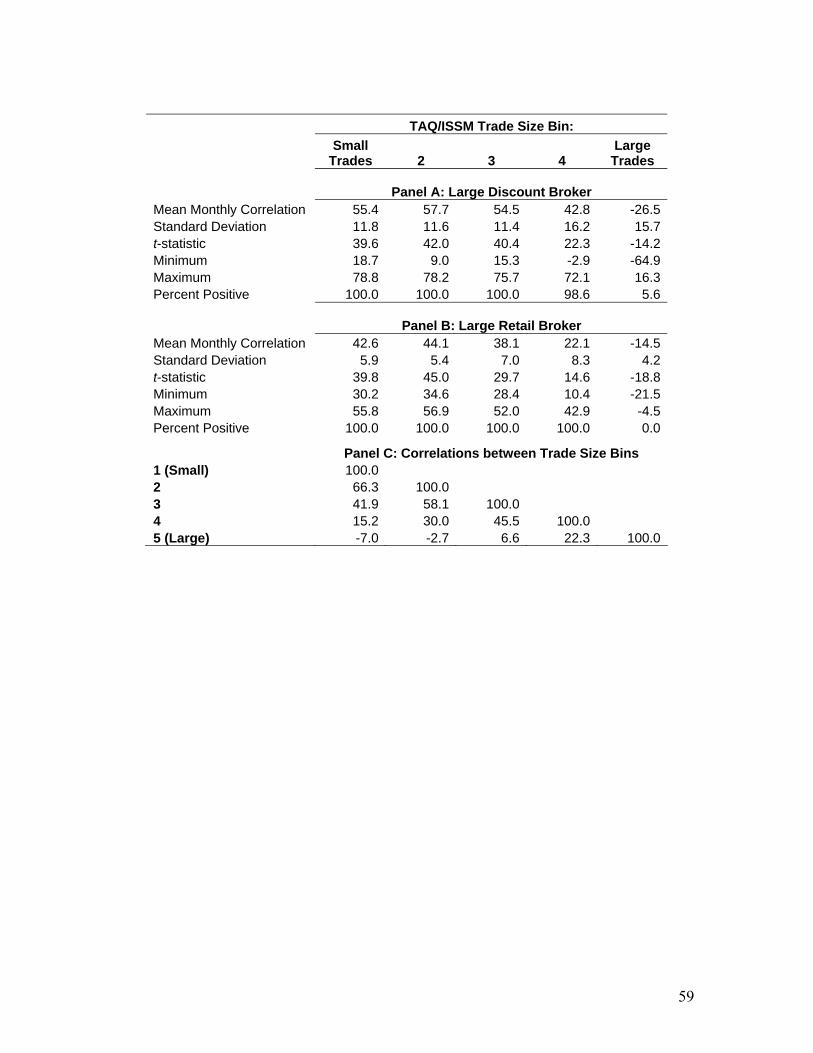
59

TAQ/ISSM Trade Size Bin:

Small

Trades 2 3 4 Large

Trades

Panel A: Large Discount Broker Mean Monthly Correlation 55.4 57.7 54.5 42.8 -26.5Standard Deviation 11.8 11.6 11.4 16.2 15.7t-statistic 39.6 42.0 40.4 22.3 -14.2Minimum 18.7 9.0 15.3 -2.9 -64.9Maximum 78.8 78.2 75.7 72.1 16.3Percent Positive 100.0 100.0 100.0 98.6 5.6

Panel B: Large Retail Broker Mean Monthly Correlation 42.6 44.1 38.1 22.1 -14.5Standard Deviation 5.9 5.4 7.0 8.3 4.2t-statistic 39.8 45.0 29.7 14.6 -18.8Minimum 30.2 34.6 28.4 10.4 -21.5Maximum 55.8 56.9 52.0 42.9 -4.5Percent Positive 100.0 100.0 100.0 100.0 0.0

Panel C: Correlations between Trade Size Bins 1 (Small) 100.0 2 66.3 100.0 3 41.9 58.1 100.0 4 15.2 30.0 45.5 100.0 5 (Large) -7.0 -2.7 6.6 22.3 100.0

60

Table 2: Descriptive Statistics for Quintiles based on Annual Proportion Buys

Quintiles are formed on the basis of annual proportion buyer-initiated transactions for

small trades (Panel A) and large trades (Panel B) from 1983 through 2000. The table

presents means across all stock-year observations. Market cap is average month-end

market cap in the ranking year. Annual turnover is total CRSP dollar volume during the

year scaled by market cap. Mean monthly market-adjusted returns are time series means

for portfolios constructed in the ranking year.

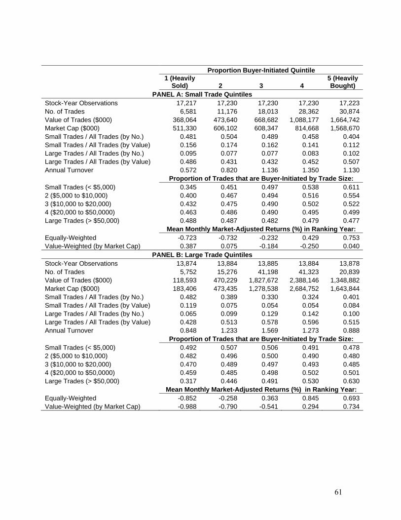
61

Proportion Buyer-Initiated Quintile

1 (Heavily

Sold) 2 3 4 5 (Heavily Bought)

PANEL A: Small Trade Quintiles Stock-Year Observations 17,217 17,230 17,230 17,230 17,223No. of Trades 6,581 11,176 18,013 28,362 30,874Value of Trades ($000) 368,064 473,640 668,682 1,088,177 1,664,742Market Cap ($000) 511,330 606,102 608,347 814,668 1,568,670Small Trades / All Trades (by No.) 0.481 0.504 0.489 0.458 0.404Small Trades / All Trades (by Value) 0.156 0.174 0.162 0.141 0.112Large Trades / All Trades (by No.) 0.095 0.077 0.077 0.083 0.102Large Trades / All Trades (by Value) 0.486 0.431 0.432 0.452 0.507Annual Turnover 0.572 0.820 1.136 1.350 1.130 Proportion of Trades that are Buyer-Initiated by Trade Size: Small Trades (< $5,000) 0.345 0.451 0.497 0.538 0.6112 ($5,000 to $10,000) 0.400 0.467 0.494 0.516 0.5543 ($10,000 to $20,000) 0.432 0.475 0.490 0.502 0.5224 ($20,000 to $50,0000) 0.463 0.486 0.490 0.495 0.499Large Trades (> $50,000) 0.488 0.487 0.482 0.479 0.477 Mean Monthly Market-Adjusted Returns (%) in Ranking Year: Equally-Weighted -0.723 -0.732 -0.232 0.429 0.753Value-Weighted (by Market Cap) 0.387 0.075 -0.184 -0.250 0.040

PANEL B: Large Trade Quintiles Stock-Year Observations 13,874 13,884 13,885 13,884 13,878No. of Trades 5,752 15,276 41,198 41,323 20,839Value of Trades ($000) 118,593 470,229 1,827,672 2,388,146 1,348,882Market Cap ($000) 183,406 473,435 1,278,538 2,684,752 1,643,844Small Trades / All Trades (by No.) 0.482 0.389 0.330 0.324 0.401Small Trades / All Trades (by Value) 0.119 0.075 0.054 0.054 0.084Large Trades / All Trades (by No.) 0.065 0.099 0.129 0.142 0.100Large Trades / All Trades (by Value) 0.428 0.513 0.578 0.596 0.515Annual Turnover 0.848 1.233 1.569 1.273 0.888 Proportion of Trades that are Buyer-Initiated by Trade Size: Small Trades (< $5,000) 0.492 0.507 0.506 0.491 0.4782 ($5,000 to $10,000) 0.482 0.496 0.500 0.490 0.4803 ($10,000 to $20,000) 0.470 0.489 0.497 0.493 0.4854 ($20,000 to $50,0000) 0.459 0.485 0.498 0.502 0.501Large Trades (> $50,000) 0.317 0.446 0.491 0.530 0.630 Mean Monthly Market-Adjusted Returns (%) in Ranking Year: Equally-Weighted -0.852 -0.258 0.363 0.845 0.693Value-Weighted (by Market Cap) -0.988 -0.790 -0.541 0.294 0.734

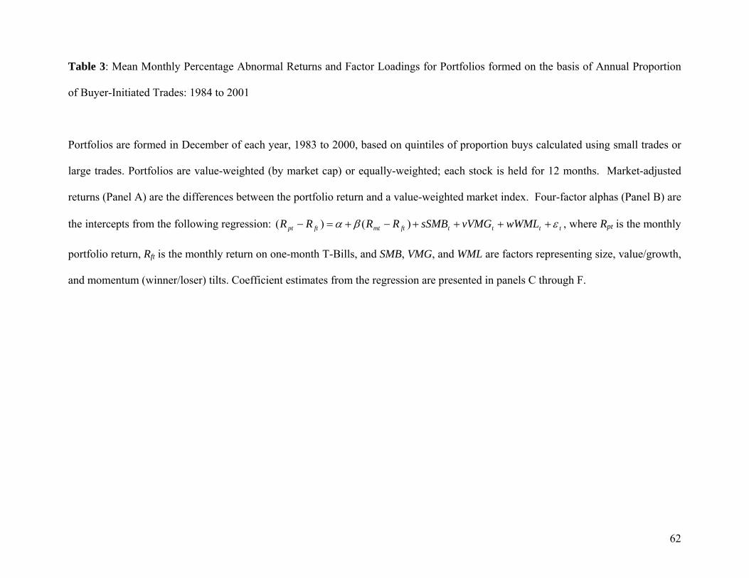
62

Table 3: Mean Monthly Percentage Abnormal Returns and Factor Loadings for Portfolios formed on the basis of Annual Proportion

of Buyer-Initiated Trades: 1984 to 2001

Portfolios are formed in December of each year, 1983 to 2000, based on quintiles of proportion buys calculated using small trades or

large trades. Portfolios are value-weighted (by market cap) or equally-weighted; each stock is held for 12 months. Market-adjusted

returns (Panel A) are the differences between the portfolio return and a value-weighted market index. Four-factor alphas (Panel B) are

the intercepts from the following regression: ttttftmtftpt wWMLvVMGsSMBRRRR εβα ++++−+=− )()( , where Rpt is the monthly

portfolio return, Rft is the monthly return on one-month T-Bills, and SMB, VMG, and WML are factors representing size, value/growth,

and momentum (winner/loser) tilts. Coefficient estimates from the regression are presented in panels C through F.

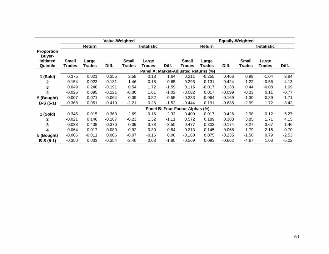
63

Value-Weighted Equally-Weighted Return t-statistic Return t-statistic Proportion

Buyer-Initiated Quintile

Small Trades

Large Trades Diff.

Small Trades

Large Trades Diff.

Small Trades

Large Trades Diff.

Small Trades

Large Trades Diff.

Panel A: Market-Adjusted Returns (%) 1 (Sold) 0.375 0.021 0.355 2.58 0.13 1.64 0.211 -0.255 0.466 0.99 -1.04 3.84

2 0.154 0.023 0.131 1.46 0.15 0.65 0.293 -0.131 0.424 1.22 -0.56 4.133 0.049 0.240 -0.191 0.54 1.72 -1.59 0.116 -0.017 0.133 0.44 -0.08 1.094 -0.026 0.095 -0.121 -0.30 1.61 -1.02 -0.082 0.017 -0.099 -0.33 0.11 -0.77

5 (Bought) 0.007 0.071 -0.064 0.09 0.82 -0.55 -0.233 -0.064 -0.169 -1.30 -0.39 -1.71B-S (5-1) -0.368 0.051 -0.419 -2.21 0.26 -1.52 -0.444 0.191 -0.635 -2.99 1.72 -3.42

Panel B: Four-Factor Alphas (%) 1 (Sold) 0.345 -0.015 0.360 2.69 -0.16 2.33 0.409 -0.017 0.426 2.98 -0.12 5.27

2 -0.021 0.146 -0.167 -0.23 1.32 -1.11 0.572 0.189 0.383 3.85 1.71 4.153 0.033 0.409 -0.376 0.39 3.73 -3.50 0.477 0.303 0.174 3.27 3.67 1.464 -0.064 0.017 -0.080 -0.92 0.30 -0.84 0.213 0.145 0.068 1.79 2.15 0.70

5 (Bought) -0.006 -0.011 0.006 -0.07 -0.16 0.06 -0.160 0.075 -0.235 -1.50 0.79 -2.53B-S (5-1) -0.350 0.003 -0.354 -2.40 0.03 -1.80 -0.569 0.093 -0.662 -4.67 1.03 -5.02

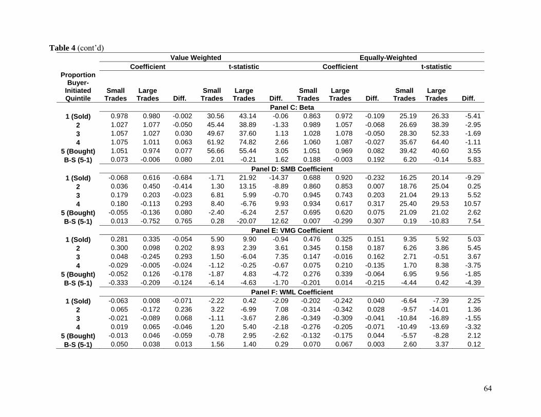
64

Table 4 (cont’d) Value Weighted Equally-Weighted Coefficient t-statistic Coefficient t-statistic Proportion

Buyer-Initiated Quintile

Small Trades

Large Trades Diff.

Small Trades

Large Trades Diff.

Small Trades

Large Trades Diff.

Small Trades

Large Trades Diff.

Panel C: Beta 1 (Sold) 0.978 0.980 -0.002 30.56 43.14 -0.06 0.863 0.972 -0.109 25.19 26.33 -5.41

2 1.027 1.077 -0.050 45.44 38.89 -1.33 0.989 1.057 -0.068 26.69 38.39 -2.953 1.057 1.027 0.030 49.67 37.60 1.13 1.028 1.078 -0.050 28.30 52.33 -1.694 1.075 1.011 0.063 61.92 74.82 2.66 1.060 1.087 -0.027 35.67 64.40 -1.11

5 (Bought) 1.051 0.974 0.077 56.66 55.44 3.05 1.051 0.969 0.082 39.42 40.60 3.55B-S (5-1) 0.073 -0.006 0.080 2.01 -0.21 1.62 0.188 -0.003 0.192 6.20 -0.14 5.83

Panel D: SMB Coefficient 1 (Sold) -0.068 0.616 -0.684 -1.71 21.92 -14.37 0.688 0.920 -0.232 16.25 20.14 -9.29

2 0.036 0.450 -0.414 1.30 13.15 -8.89 0.860 0.853 0.007 18.76 25.04 0.253 0.179 0.203 -0.023 6.81 5.99 -0.70 0.945 0.743 0.203 21.04 29.13 5.524 0.180 -0.113 0.293 8.40 -6.76 9.93 0.934 0.617 0.317 25.40 29.53 10.57

5 (Bought) -0.055 -0.136 0.080 -2.40 -6.24 2.57 0.695 0.620 0.075 21.09 21.02 2.62B-S (5-1) 0.013 -0.752 0.765 0.28 -20.07 12.62 0.007 -0.299 0.307 0.19 -10.83 7.54

Panel E: VMG Coefficient 1 (Sold) 0.281 0.335 -0.054 5.90 9.90 -0.94 0.476 0.325 0.151 9.35 5.92 5.03

2 0.300 0.098 0.202 8.93 2.39 3.61 0.345 0.158 0.187 6.26 3.86 5.453 0.048 -0.245 0.293 1.50 -6.04 7.35 0.147 -0.016 0.162 2.71 -0.51 3.674 -0.029 -0.005 -0.024 -1.12 -0.25 -0.67 0.075 0.210 -0.135 1.70 8.38 -3.75

5 (Bought) -0.052 0.126 -0.178 -1.87 4.83 -4.72 0.276 0.339 -0.064 6.95 9.56 -1.85B-S (5-1) -0.333 -0.209 -0.124 -6.14 -4.63 -1.70 -0.201 0.014 -0.215 -4.44 0.42 -4.39

Panel F: WML Coefficient 1 (Sold) -0.063 0.008 -0.071 -2.22 0.42 -2.09 -0.202 -0.242 0.040 -6.64 -7.39 2.25

2 0.065 -0.172 0.236 3.22 -6.99 7.08 -0.314 -0.342 0.028 -9.57 -14.01 1.363 -0.021 -0.089 0.068 -1.11 -3.67 2.86 -0.349 -0.309 -0.041 -10.84 -16.89 -1.554 0.019 0.065 -0.046 1.20 5.40 -2.18 -0.276 -0.205 -0.071 -10.49 -13.69 -3.32

5 (Bought) -0.013 0.046 -0.059 -0.78 2.95 -2.62 -0.132 -0.175 0.044 -5.57 -8.28 2.12B-S (5-1) 0.050 0.038 0.013 1.56 1.40 0.29 0.070 0.067 0.003 2.60 3.37 0.12

65

Table 5: Monthly Percentage Abnormal Returns for Portfolios formed from Five-by-Five Partition on Annual Proportion Buyer-

Initiated Trades based on Small Trades (columns) and Large Trades (Rows): 1984 to 2001

Portfolios are formed in December of each year, 1983 to 2000, based on independent quintiles of proportion buyer-initiated trades

calculated using small trades or large trades. Portfolios are value-weighted (by market cap); each stock is held for 12 months. Four-

factor alphas (Panel B) are the intercepts from the time-series regressions of the excess portfolio return on factors related to the

market, size, book-to-market (value/growth), and momentum.

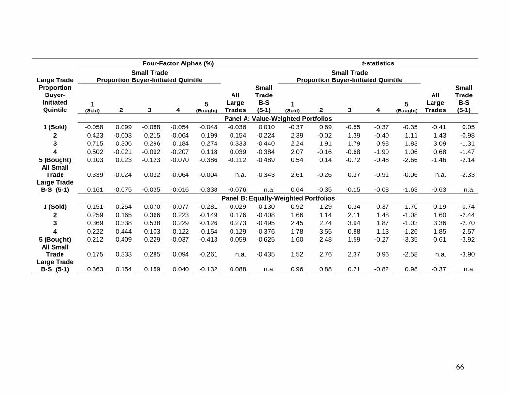
66

Four-Factor Alphas (%) t-statistics Small Trade

Proportion Buyer-Initiated Quintile Small Trade

Proportion Buyer-Initiated Quintile Large Trade Proportion

Buyer-Initiated Quintile

1 (Sold) 2 3 4

5 (Bought)

All Large

Trades

Small Trade B-S (5-1)

1 (Sold) 2 3 4

5 (Bought)

All Large

Trades

Small Trade B-S (5-1)

Panel A: Value-Weighted Portfolios 1 (Sold) -0.058 0.099 -0.088 -0.054 -0.048 -0.036 0.010 -0.37 0.69 -0.55 -0.37 -0.35 -0.41 0.05

2 0.423 -0.003 0.215 -0.064 0.199 0.154 -0.224 2.39 -0.02 1.39 -0.40 1.11 1.43 -0.983 0.715 0.306 0.296 0.184 0.274 0.333 -0.440 2.24 1.91 1.79 0.98 1.83 3.09 -1.314 0.502 -0.021 -0.092 -0.207 0.118 0.039 -0.384 2.07 -0.16 -0.68 -1.90 1.06 0.68 -1.47

5 (Bought) 0.103 0.023 -0.123 -0.070 -0.386 -0.112 -0.489 0.54 0.14 -0.72 -0.48 -2.66 -1.46 -2.14All Small

Trade 0.339 -0.024 0.032 -0.064 -0.004 n.a. -0.343 2.61 -0.26 0.37 -0.91 -0.06 n.a. -2.33Large Trade

B-S (5-1) 0.161 -0.075 -0.035 -0.016 -0.338 -0.076 n.a. 0.64 -0.35 -0.15 -0.08 -1.63 -0.63 n.a. Panel B: Equally-Weighted Portfolios

1 (Sold) -0.151 0.254 0.070 -0.077 -0.281 -0.029 -0.130 -0.92 1.29 0.34 -0.37 -1.70 -0.19 -0.742 0.259 0.165 0.366 0.223 -0.149 0.176 -0.408 1.66 1.14 2.11 1.48 -1.08 1.60 -2.443 0.369 0.338 0.538 0.229 -0.126 0.273 -0.495 2.45 2.74 3.94 1.87 -1.03 3.36 -2.704 0.222 0.444 0.103 0.122 -0.154 0.129 -0.376 1.78 3.55 0.88 1.13 -1.26 1.85 -2.57

5 (Bought) 0.212 0.409 0.229 -0.037 -0.413 0.059 -0.625 1.60 2.48 1.59 -0.27 -3.35 0.61 -3.92All Small

Trade 0.175 0.333 0.285 0.094 -0.261 n.a. -0.435 1.52 2.76 2.37 0.96 -2.58 n.a. -3.90Large Trade

B-S (5-1) 0.363 0.154 0.159 0.040 -0.132 0.088 n.a. 0.96 0.88 0.21 -0.82 0.98 -0.37 n.a.

67

Table 6: Monthly Percentage Abnormal Returns by Idiosyncratic Risk Partitions for

Value-Weighted Portfolios formed on the basis of Annual Proportion Buyer-Initiated

Trades using Small and Large Trades: 1984 to 2001

Portfolios of low, medium, and high idiosyncratic risk are formed in December of each

year, 1983 to 2000, based on quintiles of proportion buyer-initiated trades calculated

using small trades or large trades. Idiosyncratic risk is measured as the residual standard

deviation from a regression of firm returns less the risk-free rate on the market return less

the risk-free rate over four years preceding the ranking month. Stocks are ranked into

low (bottom 30%), medium (middle 40%), and high (top 30%) idiosyncratic risk

partitions. Four-factor alphas are the intercepts from the time-series regressions of the

excess portfolio return on factors related to the market, size, book-to-market

(value/growth), and momentum.

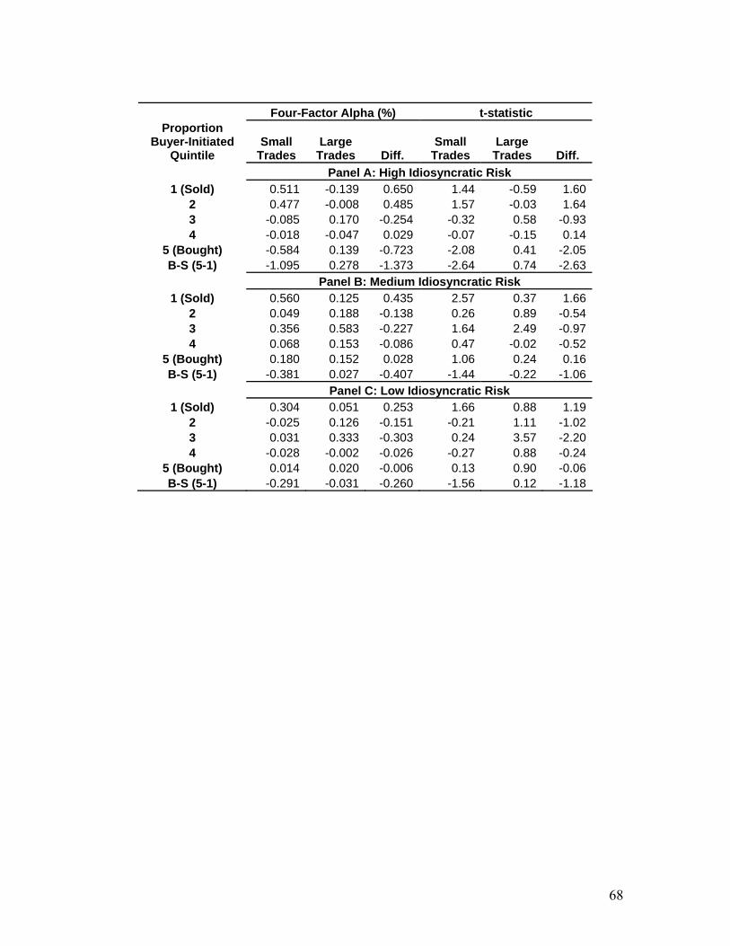
68

Four-Factor Alpha (%) t-statistic

Proportion Buyer-Initiated

Quintile Small

Trades Large

Trades Diff. Small

Trades Large Trades Diff.

Panel A: High Idiosyncratic Risk 1 (Sold) 0.511 -0.139 0.650 1.44 -0.59 1.60

2 0.477 -0.008 0.485 1.57 -0.03 1.64 3 -0.085 0.170 -0.254 -0.32 0.58 -0.93 4 -0.018 -0.047 0.029 -0.07 -0.15 0.14

5 (Bought) -0.584 0.139 -0.723 -2.08 0.41 -2.05 B-S (5-1) -1.095 0.278 -1.373 -2.64 0.74 -2.63

Panel B: Medium Idiosyncratic Risk 1 (Sold) 0.560 0.125 0.435 2.57 0.37 1.66

2 0.049 0.188 -0.138 0.26 0.89 -0.54 3 0.356 0.583 -0.227 1.64 2.49 -0.97 4 0.068 0.153 -0.086 0.47 -0.02 -0.52

5 (Bought) 0.180 0.152 0.028 1.06 0.24 0.16 B-S (5-1) -0.381 0.027 -0.407 -1.44 -0.22 -1.06

Panel C: Low Idiosyncratic Risk 1 (Sold) 0.304 0.051 0.253 1.66 0.88 1.19

2 -0.025 0.126 -0.151 -0.21 1.11 -1.02 3 0.031 0.333 -0.303 0.24 3.57 -2.20 4 -0.028 -0.002 -0.026 -0.27 0.88 -0.24

5 (Bought) 0.014 0.020 -0.006 0.13 0.90 -0.06 B-S (5-1) -0.291 -0.031 -0.260 -1.56 0.12 -1.18

69

Table 7: Percentage Abnormal Returns by Small Trade Turnover for Value-Weighted

Portfolios formed on the basis of Annual Proportion Buyer-Initiated Trades using Small

and Large Trades: 1984 to 2001

Portfolios of low, mid, and high small trade turnover are formed in December of each

year, 1983 to 2000, based on quintiles of proportion buyer-initiated trades calculated

using small trades or large trades. Small trade turnover is calculated as the total value of

small trades in the ranking year divided by mean monthly market cap. Low small trade

turnover firms are those below the 30th percentile within the year, while high small trade

turnover firms are those above the 70th percentile within the year. Remaining firms are

classified as mid small trade turnover. Portfolios are value-weighted (by market cap);

each stock is held for 12 months. Four-factor alphas (Panel B) are the intercepts from the

time-series regressions of the excess portfolio return on factors related to the market, size,

book-to-market (value/growth), and momentum.

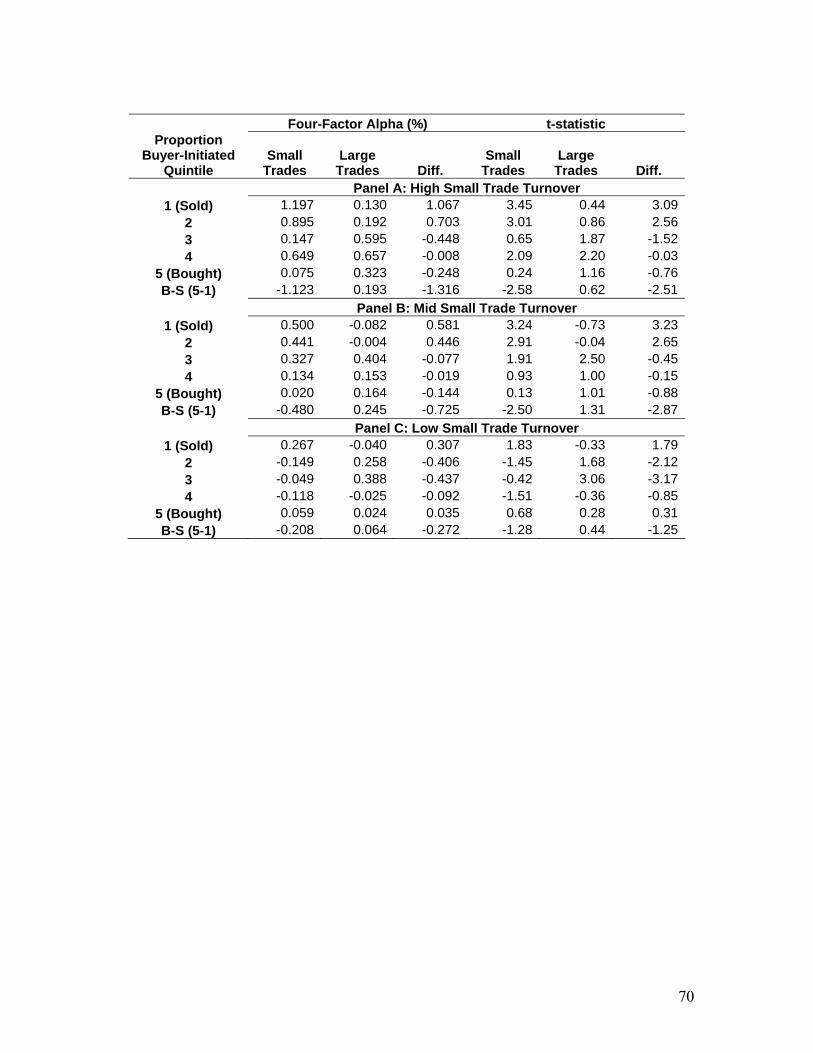
70

Four-Factor Alpha (%) t-statistic

Proportion Buyer-Initiated

Quintile Small

Trades Large Trades Diff.

Small Trades

Large Trades Diff.

Panel A: High Small Trade Turnover 1 (Sold) 1.197 0.130 1.067 3.45 0.44 3.09

2 0.895 0.192 0.703 3.01 0.86 2.563 0.147 0.595 -0.448 0.65 1.87 -1.524 0.649 0.657 -0.008 2.09 2.20 -0.03

5 (Bought) 0.075 0.323 -0.248 0.24 1.16 -0.76B-S (5-1) -1.123 0.193 -1.316 -2.58 0.62 -2.51

Panel B: Mid Small Trade Turnover 1 (Sold) 0.500 -0.082 0.581 3.24 -0.73 3.23

2 0.441 -0.004 0.446 2.91 -0.04 2.653 0.327 0.404 -0.077 1.91 2.50 -0.454 0.134 0.153 -0.019 0.93 1.00 -0.15

5 (Bought) 0.020 0.164 -0.144 0.13 1.01 -0.88B-S (5-1) -0.480 0.245 -0.725 -2.50 1.31 -2.87

Panel C: Low Small Trade Turnover 1 (Sold) 0.267 -0.040 0.307 1.83 -0.33 1.79

2 -0.149 0.258 -0.406 -1.45 1.68 -2.123 -0.049 0.388 -0.437 -0.42 3.06 -3.174 -0.118 -0.025 -0.092 -1.51 -0.36 -0.85

5 (Bought) 0.059 0.024 0.035 0.68 0.28 0.31B-S (5-1) -0.208 0.064 -0.272 -1.28 0.44 -1.25

71

Table 8: Monthly Percentage Abnormal Returns for Value-Weighted Portfolios formed

on the basis of Weekly Proportion Buyer-Initiated Trades using Small and Large Trades:

February 1983 to December 2000

Portfolios are formed on Wednesday of each week, 1/4/1983 to 12/27/2000, based on

quintiles of weekly proportion buyer-initiated trades calculated using small trades or

large trades. In Panel A, positions are taken the first day of the ranking period and held

for the ranking period (i.e., one week). In Panel B, positions are taken the day after

ranking and held for one week (five trading days). The daily returns of portfolios are

compounded to yield a monthly return series. Four-factor alphas are the intercepts from

the time-series regressions of the monthly excess portfolio return on factors related to the

market, size, book-to-market (value/growth), and momentum.

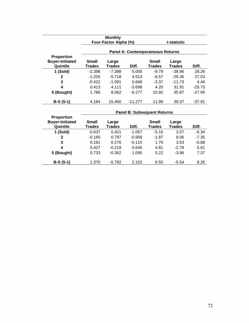
72

Monthly

Four-Factor Alpha (%) t-statistic

Panel A: Contemporaneous Returns Proportion

Buyer-Initiated Quintile

Small Trades

Large Trades Diff.

Small Trades

Large Trades Diff.

1 (Sold) -2.398 -7.398 5.000 -9.79 -38.96 28.262 -1.205 -5.718 4.513 -6.57 -29.36 27.033 -0.422 -1.091 0.668 -3.37 -11.73 4.464 0.413 4.111 -3.698 4.20 31.91 -25.73

5 (Bought) 1.786 8.062 -6.277 10.92 35.87 -27.95

B-S (5-1) 4.184 15.460 -11.277 11.99 39.37 -37.91

Panel B: Subsequent Returns Proportion

Buyer-Initiated Quintile

Small Trades

Large Trades Diff.

Small Trades

Large Trades Diff.

1 (Sold) -0.637 0.421 -1.057 -5.16 3.57 -6.342 -0.160 0.797 -0.958 -1.87 8.06 -7.353 0.161 0.276 -0.115 1.70 3.53 -0.884 0.427 -0.219 0.646 4.81 -2.79 5.61

5 (Bought) 0.733 -0.362 1.095 5.22 -3.96 7.37

B-S (5-1) 1.370 -0.782 2.152 6.55 -5.54 8.26

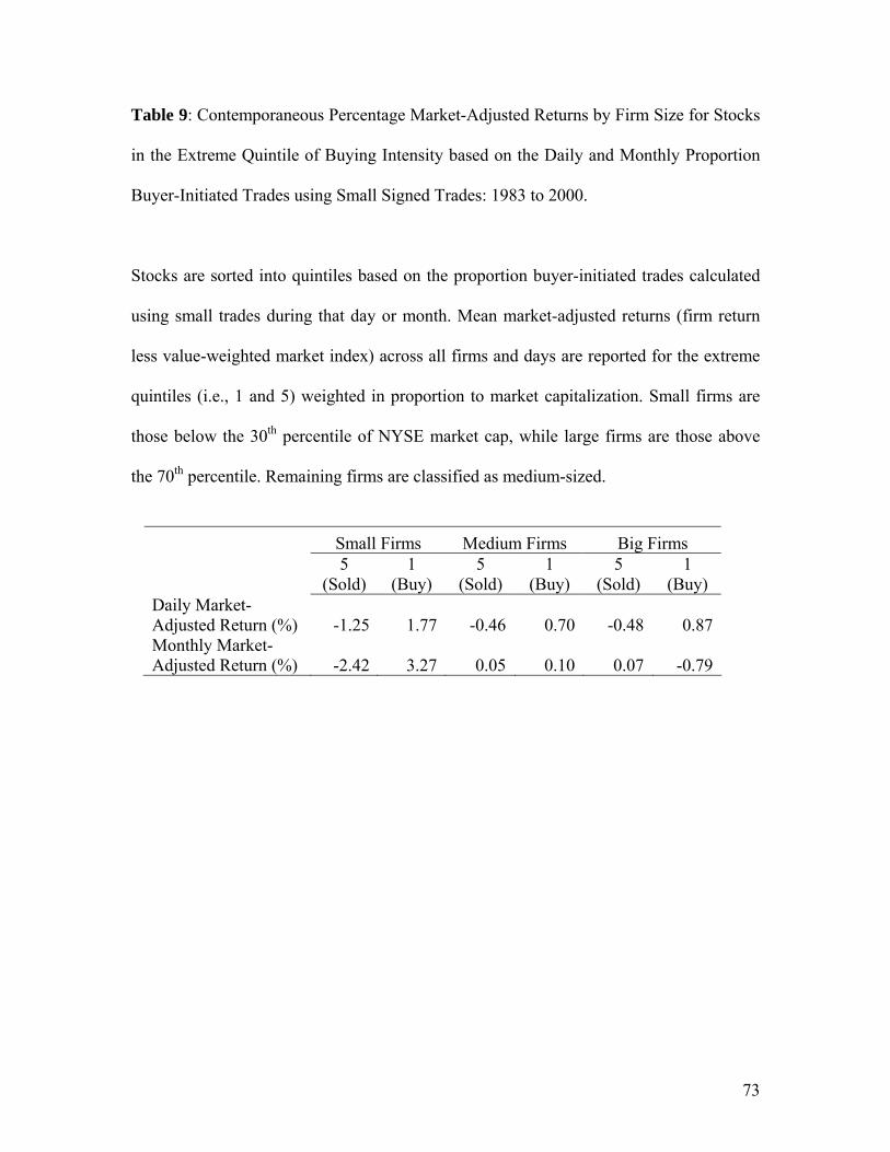
73

Table 9: Contemporaneous Percentage Market-Adjusted Returns by Firm Size for Stocks

in the Extreme Quintile of Buying Intensity based on the Daily and Monthly Proportion

Buyer-Initiated Trades using Small Signed Trades: 1983 to 2000.

Stocks are sorted into quintiles based on the proportion buyer-initiated trades calculated

using small trades during that day or month. Mean market-adjusted returns (firm return

less value-weighted market index) across all firms and days are reported for the extreme

quintiles (i.e., 1 and 5) weighted in proportion to market capitalization. Small firms are

those below the 30th percentile of NYSE market cap, while large firms are those above

the 70th percentile. Remaining firms are classified as medium-sized.

Small Firms Medium Firms Big Firms

5

(Sold) 1

(Buy) 5

(Sold) 1

(Buy) 5

(Sold) 1

(Buy) Daily Market-Adjusted Return (%) -1.25 1.77 -0.46 0.70 -0.48 0.87 Monthly Market-Adjusted Return (%) -2.42 3.27 0.05 0.10 0.07 -0.79

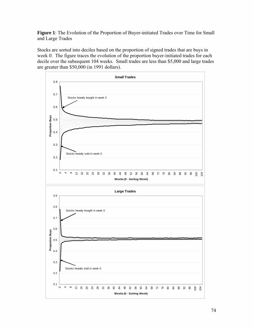
74

Figure 1: The Evolution of the Proportion of Buyer-initiated Trades over Time for Small and Large Trades Stocks are sorted into deciles based on the proportion of signed trades that are buys in week 0. The figure traces the evolution of the proportion buyer-initiated trades for each decile over the subsequent 104 weeks. Small trades are less than $5,000 and large trades are greater than $50,000 (in 1991 dollars).

Small Trades

0.1

0.2

0.3

0.4

0.5

0.6

0.7

0.8

0 4 8 12 16 20 24 28 32 36 40 44 48 52 56 60 64 68 72 76 80 84 88 92 96 100

104

Weeks (0 - Sorting Week)

Prop

ortio

n Bu

ys

Large Trades

0.1

0.2

0.3

0.4

0.5

0.6

0.7

0.8

0.9

0 4 8 12 16 20 24 28 32 36 40 44 48 52 56 60 64 68 72 76 80 84 88 92 96 100

104

Weeks (0 - Sorting Week)

Prop

ortio

n Bu

ys

Stocks heavily bought in week 0

Stocks heavily sold in week 0

Stocks heavily sold in week 0

Stocks heavily bought in week 0

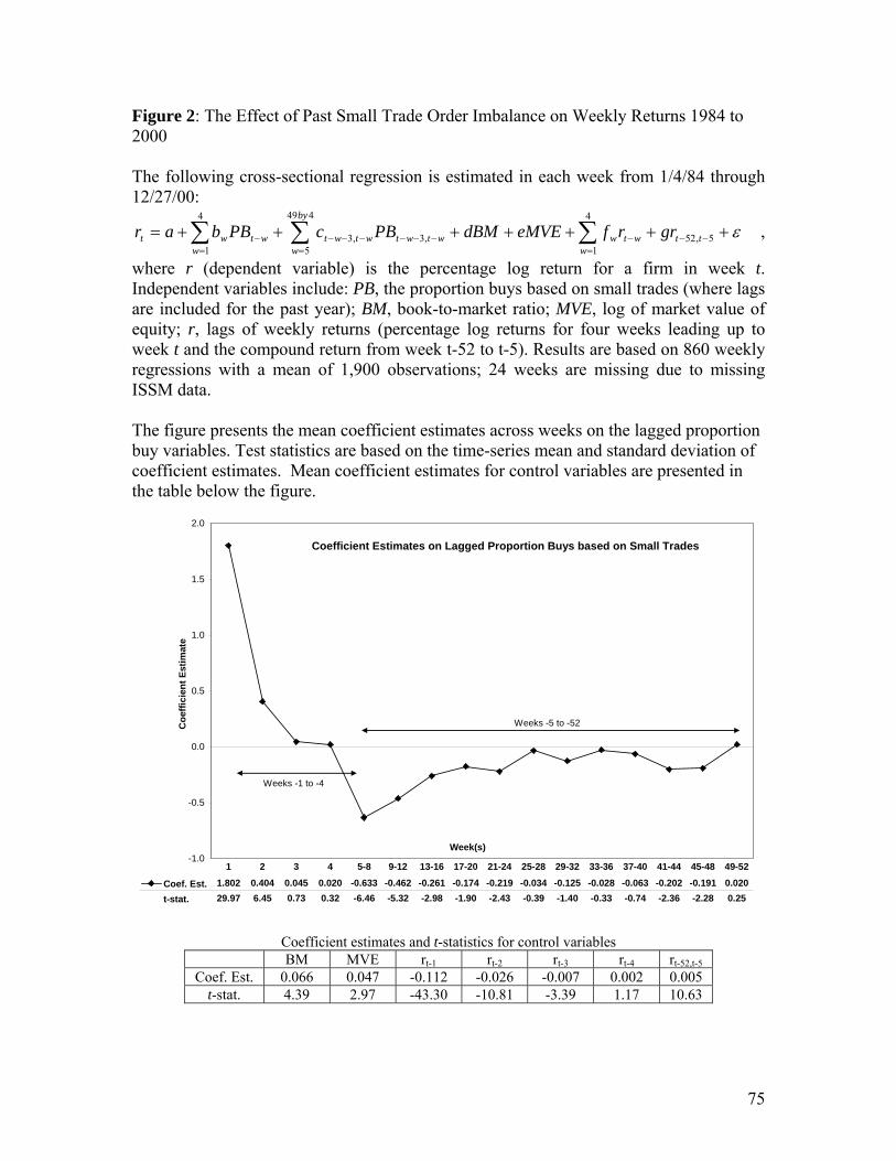
75

Figure 2: The Effect of Past Small Trade Order Imbalance on Weekly Returns 1984 to 2000 The following cross-sectional regression is estimated in each week from 1/4/84 through 12/27/00:

∑ ∑∑= =

−−−−−−−−−−=

+++++++=449

5

4

15,52,3,3

4

1

by

w wttwtwwtwtwtwtwt

wwt grrfeMVEdBMPBcPBbar ε ,

where r (dependent variable) is the percentage log return for a firm in week t. Independent variables include: PB, the proportion buys based on small trades (where lags are included for the past year); BM, book-to-market ratio; MVE, log of market value of equity; r, lags of weekly returns (percentage log returns for four weeks leading up to week t and the compound return from week t-52 to t-5). Results are based on 860 weekly regressions with a mean of 1,900 observations; 24 weeks are missing due to missing ISSM data. The figure presents the mean coefficient estimates across weeks on the lagged proportion buy variables. Test statistics are based on the time-series mean and standard deviation of coefficient estimates. Mean coefficient estimates for control variables are presented in the table below the figure.

Coefficient Estimates on Lagged Proportion Buys based on Small Trades

-1.0

-0.5

0.0

0.5

1.0

1.5

2.0

Week(s)

Coe

ffici

ent E

stim

ate

Coef. Est. 1.802 0.404 0.045 0.020 -0.633 -0.462 -0.261 -0.174 -0.219 -0.034 -0.125 -0.028 -0.063 -0.202 -0.191 0.020t-stat. 29.97 6.45 0.73 0.32 -6.46 -5.32 -2.98 -1.90 -2.43 -0.39 -1.40 -0.33 -0.74 -2.36 -2.28 0.25

1 2 3 4 5-8 9-12 13-16 17-20 21-24 25-28 29-32 33-36 37-40 41-44 45-48 49-52

Weeks -1 to -4

Weeks -5 to -52

Coefficient estimates and t-statistics for control variables

BM MVE rt-1 rt-2 rt-3 rt-4 rt-52,t-5 Coef. Est. 0.066 0.047 -0.112 -0.026 -0.007 0.002 0.005

t-stat. 4.39 2.97 -43.30 -10.81 -3.39 1.17 10.63

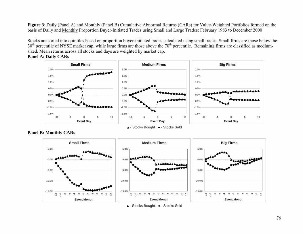
76

Figure 3: Daily (Panel A) and Monthly (Panel B) Cumulative Abnormal Returns (CARs) for Value-Weighted Portfolios formed on the basis of Daily and Monthly Proportion Buyer-Initiated Trades using Small and Large Trades: February 1983 to December 2000 Stocks are sorted into quintiles based on proportion buyer-initiated trades calculated using small trades. Small firms are those below the 30th percentile of NYSE market cap, while large firms are those above the 70th percentile. Remaining firms are classified as medium-sized. Mean returns across all stocks and days are weighted by market cap. Panel A: Daily CARs

▲ - Stocks Bought ● - Stocks Sold

Medium Firms

-1.5%

-1.0%

-0.5%

0.0%

0.5%

1.0%

1.5%

2.0%

-10 -5 0 5 10

Event Day

Small Firms

-1.5%

-1.0%

-0.5%

0.0%

0.5%

1.0%

1.5%

2.0%

-10 -5 0 5 10

Event Day

Big Firms

-1.5%

-1.0%

-0.5%

0.0%

0.5%

1.0%

1.5%

2.0%

-10 -5 0 5 10

Event Day

Panel B: Monthly CARs

▲ - Stocks Bought ● - Stocks Sold

Small Firms

-15.0%

-10.0%

-5.0%

0.0%

5.0%

-12

-10 -8 -6 -4 -2 0 2 4 6 8 10 12

Event Month

Medium Firms

-15.0%

-10.0%

-5.0%

0.0%

5.0%

-12

-10 -8 -6 -4 -2 0 2 4 6 8 10 12

Event Month

Big Firms

-15.0%

-10.0%

-5.0%

0.0%

5.0%

-12

-10 -8 -6 -4 -2 0 2 4 6 8 10 12

Event Month