RESEARCHPAPER

Do species distribution models explainspatial structure within tree speciesranges?geb_478 662..673

Daniel Montoya1*, Drew W. Purves2, Itziar R. Urbieta1,3 and

Miguel A. Zavala4

1Departamento de Ecología, Universidad de

Alcalá, 28871 Alcalá de Henares, Madrid,

Spain, 2Microsoft Research Cambridge, 7 J J

Thomson Avenue, Cambridge CB3 0FB, UK,3IRNA, CSIC, PO Box 1052, E-41080, Sevilla,

Spain, 4Centro de Investigación Forestal

(CIFOR), Instituto Nacional de Investigación y

Tecnología Agraria y Alimentaria (INIA),

28040 Madrid, Spain

ABSTRACT

Aim To evaluate the ability of species distribution models (SDMs) to predict thespatial structure of tree species within their geographical ranges (how trees aredistributed within their ranges).

Location Continental Spain.

Methods We used an extensive dataset consisting of c. 90,000 plots (1 plot km-2)where presence/absence data for 23 common Mediterranean and Atlantic treespecies had been surveyed. We first generated SDMs relating the presence orabsence of each species to a set of 16 environmental predictors, following a stepwisemodelling process based on maximum likelihood methods. Superimposing spatialcorrelograms generated from the predictions of the SDMs over those generatedfrom the raw data allowed a model–observation comparison of the nature, scaleand intensity (level of aggregation) of spatial structure with the species ranges.

Results SDMs predicted accurately the nature and scale of the spatial structure oftrees. However, for most species, the observed intensity of spatial structure (level ofaggregation of species in space) was substantially greater than that predicted by theSDMs. On average, the intensity of spatial aggregation was twice that predicted bySDMs. In addition, we also found a negative correlation between intensity ofaggregation and species range size.

Main conclusions Standard SDM predictions of spatial structure patterns differamong species. SDMs are apparently able to reproduce both the scale and intensityof species spatial structure within their ranges. However, one or more missingprocesses not included in SDMs results in species being substantially more aggre-gated in space than can be captured by the SDMs. This result adds to recent calls fora new generation of more biologically realistic SDMs. In particular, future SDMsshould incorporate ecological processes that are likely to increase the intensity ofspatial aggregation, such as source–sink dynamics, fine-scale environmental het-erogeneity and disequilibrium.

KeywordsCovariance–distance function, Iberian Peninsula, maximum likelihood, spatialstructure, species aggregation, species distribution models (SDMs), trees.

*Correspondence: Daniel Montoya, Departmentof Ecología, Universidad de Alcalá, 28871 Alcaláde Henares, Madrid, Spain.E-mail: daniel.montoya@alu.uah.es

INTRODUCTION

Anthropogenic climate change is a major threat to the mainte-

nance of biological diversity. Most modelling frameworks used

to predict its effects on species distributions rely on the biocli-

matic ‘envelope’ approach, whereby present climate–species

relationships are used to estimate distributions of species under

future climate scenarios (Huntley et al., 1995; Peterson et al.,

2002; Thomas et al., 2004; Thuiller et al., 2005). Despite recent

studies having demonstrated significant variability in model

predictions (Segurado & Araújo, 2004; Pearson et al., 2006),

species distribution models (SDMs) constitute a general and

Global Ecology and Biogeography, (Global Ecol. Biogeogr.) (2009) 18, 662–673

DOI: 10.1111/j.1466-8238.2009.00478.x© 2009 Blackwell Publishing Ltd www.blackwellpublishing.com/geb662

widely used approximation to modelling the geographical

ranges of biological communities, on the basis that climate is the

main driver of species distributions world-wide (Hawkins et al.,

2003).

One of the main criticisms of SDMs, however, is that these

models implicitly assume that biological communities are

niche-assembled and not influenced by endogenous factors

(Pearson & Dawson, 2003; Hampe, 2004). This assumption

overlooks empirical evidence showing that spatial structure

often emerges due to population-level factors (e.g. dispersal,

biotic interactions, gregarious behaviour) as well as exogenous

factors (e.g. aggregated environmental conditions; Lehman &

Tilman, 1997). Moreover, Bahn & McGill (2007) recently

showed that environmental variables captured the spatial struc-

ture of breeding birds of North America in a haphazard way,

suggesting that population-level processes rather than exog-

enous factors are the main predictors of the spatial structure

patterns of species. Although these findings do not exclude the

environment from models, they suggest that modelling species

distributions must integrate diverse sets of explanatory factors

from pure environmental variables (scenopetic; Soberón, 2007)

to resource-related and biotic variables (bionomic; Soberón,

2007), because they together generate the spatial patterns

observed in nature: scenopoetic variables may have broad spatial

structures (i.e. climate), whereas bionomic variables probably

tend to have much more fine-grained spatial structures (i.e.

biotic interactions). Given that bionomic variables are difficult

to obtain at broad geographical scales, modelling population-

level processes represents a major challenge for SDMs, and

attempts to incorporate processes such as competition and

mutualistic interactions into the SDM framework are gaining in

importance (Leathwick & Austin, 2001; Anderson et al., 2002;

Gutiérrez et al., 2005; Araújo & Luoto, 2007). Although this

research shows that the inclusion of population-level processes

improves SDMs, a remaining question is to what extent SDMs

predict the spatial structure of individual species within their

distribution ranges. This is intriguing, since knowledge of this

spatial structure is likely to be critical for understanding the

dynamics of forest communities, their interactions with the

environment and other biological species and their response to

climate changes (Lehman & Tilman, 1997).

In spatial ecology, the term ‘spatial structure’ refers to how

species are organized (structured) within their distribution

ranges by reference to a random (non-structured) null model

that is usually assumed to be a homogeneous Poisson process.

Spatial structure can be explored using a spatial covariance–

distance function (Solé & Bascompte, 2007), which provides a

measure of the direction and magnitude of deviation from ran-

domness of a pair of locations as a function of their distance

apart. This function reveals three important components of the

spatial structure that we refer to here as intensity, nature and

scale. Intensity is a quantitative measure of the magnitude of

spatial structure, i.e. the magnitude of the deviation between the

observed pattern, and the null model. Intensity is associated

with the level of aggregation/segregation of species in space, and

gives information about how close in space are individuals from

the same species. This magnitude is usually greatest at distance

0, and so in practice the intensity can usually be defined as the

value of the covariance function at distance 0. Nature refers to

the direction of the deviation (more aggregated than expected

from the null model; less aggregated than expected) and how

this changes with distance (e.g. more aggregated than expected

at short distances, less aggregated than expected at intermediate

distances, random at large distance). Scale refers to the distances

in space over which the deviation occurs (e.g. at what distance

does the pattern first become non-structured?). Therefore,

nature and scale are qualitative measures of spatial structure that

focus on questions such as whether species within a region are

equally similar regardless of distance or differ as a function of

distance.

Theory and evidence suggest that population-level processes

affect species ranges (e.g. post-glacial dispersal limitation; Sven-

ning & Skov, 2007) as well as spatial structure within these

ranges (e.g. local dispersal leads to intraspecific aggregation;

Pacala, 1997). However, little is known about what elements of

the observed spatial structure in species distributions are more

related to either environmental or population-level processes.

The most likely reason for this is that current SDMs have com-

monly focused on understanding species ranges and how these

might alter under climate change, but have rarely examined

how individual species are arranged within those ranges (e.g.

random, regular/uniform, aggregated). A fundamental issue

when exploring spatial structure is that we need models that

allow a continuous probability of occurrence of a species given

certain environmental conditions. Although most SDMs can

potentially generate such probability maps, they usually convert

a posteriori the continuous probabilities (range 0–1) into a

binary prediction for presence/absence (0 or 1). This reduces

continuous probability maps to discrete presence/absence pre-

dictions, and so spatial structure cannot be accurately studied

because ecological properties such as spatial aggregation of indi-

viduals show no patterns of response along environmental gra-

dients. Therefore, current SDMs have not yet shown how they

can capture the nature, scale and intensity of the spatial struc-

ture of individual species at finer scales.

Here, we investigate the performance of an SDM to capture

the spatial structure of 23 common tree species of Mediterra-

nean and Atlantic ecosystems. By using spatial structure analy-

sis, we evaluate the performance of SDMs to describe the

observed spatial structure for many species and at fine spatial

scales. This is potentially important for understanding species

distributions because many suggested processes that may dimin-

ish the explanatory power of SDMs mainly operate at short to

intermediate spatial scales (e.g. dispersal, biotic interactions,

perturbation events, habitat loss and fragmentation; Pearson &

Dawson, 2003; Hampe, 2004). For example, empirical dispersal

kernels show high densities of seeds at short distances from the

parent tree, demonstrating that local dispersal leads to intraspe-

cific aggregation (Pacala, 1997). Also, perturbations such as

habitat loss and fragmentation usually divide landscapes into a

set of forest patches, which in turn cause patchy aggregated

distributions of species (Fahrig, 2003). Given that most of the

SDMs and the spatial aggregation of trees

Global Ecology and Biogeography, 18, 662–673, © 2009 Blackwell Publishing Ltd 663

population-level processes not considered by SDMs tend to

result in more aggregated structures, we were interested in

testing the hypothesis that spatial aggregation is the main

unpredicted component of the spatial structure. Specifically, we

address three questions: (1) To what extent can species spatial

structure be predicted by environmental conditions? (2) How

does this predictive ability differ among different features of the

spatial structure (intensity, nature, scale)? (3) How does this

predictive ability differ among species?

DATA AND METHODS

Study region

We analysed data from an extensive dataset obtained in conti-

nental Spain (492,173 km2). This region houses a large altitudi-

nal gradient (sea level to 3500 m); it comprises a mosaic of

different climates (from semi-arid climates to Mediterranean

and humid Atlantic climates), and a number of different land-

scapes. The Second Spanish Forest Inventory (Inventario For-

estal Nacional, 1995) surveyed this area (1986–96), yielding a

total of 89,365 circular plots distributed across the forested

surface of the Iberian Peninsula, with an approximate density of

1 plot km-2. Each plot was located in the field by giving its

Universal Transverse Mercator (UTM) coordinates, and was

sampled for many attributes. We extracted the presence/absence

data for 23 tree species commonly found in Mediterranean and

Atlantic forests of the study region. These species comprise a

wide range of niches and biological traits and include both

native and introduced species (Table 1).

Environmental variables

To reduce the chance of missing environmental factors that may

explain the observed patterns, environmental variability was

characterized for each plot by a set of 16 variables which might

be critical to plant physiological function and survival in the

Mediterranean and Atlantic systems. We used annual, seasonal

and monthly values of mean temperature (T, °C) and precipi-

tation (P, mm), and annual and seasonal values of mean radia-

tion (RAD, kW m-2), extracted from a digital atlas of the Iberian

Peninsula (Ninyerola et al., 2005). From these variables, we

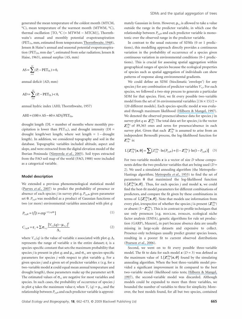
Table 1 List of tree species included inthe analyses.

Species Origin

Factor 1

(D = 1)

Factor 2

(D = 2)

Factor 3

(D = 3) d Pseudo R2

Abies alba Native MTCM SumP 0.81 0.68

Castanea sativa Exotic AnP MTCM 0.29 0.33

Ceratonia siliqua Native MTCM AHI 0.53 0.66

Corylus avellana Native SumP TO 0.32 0.68

Eucalyptus camaldulensis Exotic AMT AHI 0.24 0.55

Eucalyptus globulus Exotic TO MTCM SumP 0.53 0.44

Fagus sylvatica Native SumP TO 0.39 0.74

Ilex aquifolium Native SumP TO 0.46 0.86

Juniperus thurifera Native MTCM AnP 0.21 0.35

Olea europaea Native MTWM AMT 0.31 0.47

Phyllirea latifolia Native MTWM AnP 0.43 0.65

Pinus halepensis Native MTWM AHI 0.42 0.54

Pinus nigra Native MTCM MTWM 0.27 0.44

Pinus pinaster Native AMT TO 0.32 0.68

Pinus radiata Exotic AR MTCM 0.18 0.19

Pinus sylvestris Native AMT SprP 0.27 0.33

Pinus uncinata Native MTCM SumP MTWM 0.89 0.92

Quercus faginea Native MTCM AnP 0.39 0.49

Quercus ilex Native AnP MTCM 0.05 0.06

Quercus petraea Native SumP TO 0.20 0.27

Quercus robur Native TO SprP 0.80 0.89

Quercus suber Native AMT SprP 0.42 0.63

Rhamnus alaternus Native MTWM SumP 0.43 0.73

The origin of each species (native versus exotic) is indicated. Variables included in the best-fit speciesdistribution models (SDMs) are provided. The proportion of spatial aggregation explained by SDMsis provided for each species as the species’ predicted aggregation at distance 0 (d) and overall predictedspatial structure (pseudo R2).MTCM, mean temperature of the coldest month (°C); MTWM, mean temperature of the warmestmonth (°C); TO, thermal oscillation (°C); SumP, summer precipitation (mm); SprP, spring precipi-tation (mm); AnP, annual precipitation (mm); AMT, annual mean temperature (°C); AHI, annualhydric index (adimensional); AR, annual radiation (kW m-2). See main text for definitions and datasources.

D. Montoya et al.

Global Ecology and Biogeography, 18, 662–673, © 2009 Blackwell Publishing Ltd664

generated the mean temperature of the coldest month (MTCM,

°C), mean temperature of the warmest month (MTWM, °C),

thermal oscillation [TO, °C (= MTWM - MTCM)], Thornth-

waite’s annual and monthly potential evapotranspiration

(PETTh, mm, estimated from temperature; Thornthwaite, 1948),

Jensen & Haise’s annual and seasonal potential evapotranspira-

tion (PETJH, mm day-1, estimated from solar radiation; Jensen &

Haise, 1963), annual surplus (AS, mm)

AS PETTh= −( ) >=∑ Pi

i 1

12

0,

annual deficit (AD, mm)

AD PETTh= −( ) <=∑ Pi

i 1

12

0,

annual hydric index (AHI; Thornthwaite, 1957)

AHI AS AD PETTh= × − ×( )100 60 ,

drought length (DL = number of months where monthly pre-

cipitation is lower than PETTh), and drought intensity (DI =drought length/wet length; where wet length = 1 – drought

length). In addition, we considered topography and soil in the

database. Topographic variables included altitude, aspect and

slope, and were extracted from the digital elevation model of the

Iberian Peninsula (Ninyerola et al., 2005). Soil types extracted

from the FAO soil map of the world (FAO, 1988) were included

as a categorical variable.

Model description

We extended a previous phenomenological statistical model

(Purves et al., 2007) to predict the probability of presence or

absence of each species j in survey plot q, Pj,q,q, given parameter

set q. Pj,q,q was modelled as a product of Gaussian functions of

two (or more) environmental variables associated with plot q:

Pj qC j q

, ,, ,expθ

θ= +[ ]− ( )1 1 (1)

CV q

j q j x jx j x j

x, , ,

, ,θ ε σ

μ= + ∑

( ) −[ ]2

Δ(2)

where Vx,j(q) is the value of variable x associated with plot q; Dx

represents the range of variable x in the entire dataset; ej is a

species-specific constant that sets the maximum probability that

species j is present in plot q; and mx,j and sx,j are species-specific

parameters for species j with respect to plot variable q. For a

given species j and a given set of predictor variables x (e.g. for a

two-variable model x could equal mean annual temperature and

drought length), these parameters make up the parameter set q.

The estimated values of sx,j are negative for most variables and

species. In such cases, the probability of occurrence of species j

in plot q takes the maximum value ej when Vx (q) = mx,j and the

relationship between Pj,q,q and each predictor variable is approxi-

mately Gaussian in form. However, mx,j is allowed to take a value

outside the range in the predictor variable, in which case the

relationship between Pj,q,q and each predictor variable is mono-

tonic over the observed range in the predictor variable.

In contrast to the usual outcome of SDMs (0 or 1 predic-

tions), this modelling approach directly provides a continuous

variation in the probability of occurrence of a species given

continuous variation in environmental conditions (0–1 predic-

tions). This is crucial for assessing spatial aggregation within

geographical ranges of species because the ecological properties

of species such as spatial aggregation of individuals can show

patterns of response along environmental gradients.

We could define an SDM (bioclimatic ‘envelope’) for any

species j for any combination of predictor variables Vx,j. For each

species, we followed a two-step process to generate a particular

SDM for that species. First, we fit every possible two-variable

model from the set of 16 environmental variables [(16 ¥ 15)/2 =120 different models]. Each species-specific model x was evalu-

ated through maximum likelihood (Hilborn & Mangel, 1997).

We denoted the observed presence/absence data for species j in

survey plot q as Z j q,Obs. The total data set for species j is the vector

Z j q,Obs of 89,365 ones and zeros for presence/absence in each

survey plot. Given that each Z j q,Obs is assumed to arise from an

independent Bernoulli process, the log-likelihood function forZ j q,

Obs is:

L Obs Obs ObsZ x Zj q j q j q j q j qZ P P, , , , , , ,, ln lnθ θ θ{ } = ⋅ ( ) + −( )⋅ −( )[ 1 1 ]]∑ (3)

For two-variable models x is a vector of size D whose compo-

nents define the two predictor variables that are being used (D =2). We used a simulated annealing algorithm (the Metropolis–

Hastings algorithm; Metropolis et al., 1953) to find the set of

parameters q that maximized the log-likelihood functionL ObsZ xj q, ,θ{ } . Thus, for each species j and model x, we could

find the best-fit model parameters for different combinations of

predictors, and compare the fit given by these combinations in

terms of L ObsZ xj q, ,θ{ }. Note that models use information from

every plot, irrespective of whether the species j is present (Z j q,Obs)

or absent (1− Z j q,Obs). This is in contrast to profile techniques that

use only presences [e.g. bioclim, domain, ecological niche

factor analysis (ENFA), genetic algorithms for rule set produc-

tion (GARP), Maxent], in part because absence data are usually

missing in large-scale datasets and expensive to collect.

Presence-only techniques usually predict greater species losses,

resulting in a poorer fit to current observed distributions

(Pearson et al., 2006).

Second, we went on to fit every possible three-variable

model. The fit to data for each model x (D = 3) was defined as

the maximum value of L ObsZ xj q, ,θ{ } found by the simulating

annealing algorithm. When the best three-variable model pro-

vided a significant improvement in fit compared to the best

two-variable model (likelihood ratio tests; Hilborn & Mangel,

1997), the second-variable model was discarded. Although

models could be expanded to more than three variables, we

bounded the number of variables to three for simplicity. More-

over, the best models found, for all but two species, contained

SDMs and the spatial aggregation of trees

Global Ecology and Biogeography, 18, 662–673, © 2009 Blackwell Publishing Ltd 665

only two variables. Therefore increasing the model dimension-

ality was not justified in this case because it did not provide

further information, nor would it improve model fits statisti-

cally. Multi-collinearity was minimized by preventing SDMs

from incorporating highly correlated variables (r > 0.6).

Spatial analysis

We used spatial correlograms, which give information on the

spatial similarity of the samples versus their distance apart

(spatial covariance–distance function, Solé & Bascompte, 2007).

Spatial structure was quantified using the spatial covariance

functions given in Purves et al. (2007). These statistics give a

value for the autocovariance of species j at a distance class r,

Cj(r), which we compare with the expected correlation under

spatial randomness E{Cj(r)}. The ratio of these two quantities

yields a dimensionless measure of departure from spatial aggre-

gation Wj(r) (Condit et al., 2000). A value of Wj(r) > 0 indicates

aggregation of species j at distance class r, Wj(r) < 0 indicates

segregation, and Wj(r) = 0 indicates spatial randomness (no

aggregation or segregation). The W statistic was used because it

is simpler than the many alternative distance-based covariance

functions (e.g. semi-variance, Ripley’s k; Ripley, 1981); but it is

likely to have yielded similar results to them. The estimates of Wdo not depend on the arrangement of survey plots.

We explored the spatial autocorrelation of the observations,

and compared these with the spatial structure predicted by the

SDMs. For each species, we calculated correlograms both from

the observations and from the predictions of the best model. To

do this, we generated spatial correlograms using the spatial

covariance functions calculated for original observations and

predicted spatial structure after fitting each model at 20 distance

classes. Thus, the smaller the difference in spatial autocorrela-

tion between observed and predicted values at any distance class,

the greater the capacity of the model to explain spatial structure

at that distance. In contrast, any remaining spatial autocorrela-

tion at a distance class indicates the inadequacy of the model to

describe the spatial structure at that scale and therefore suggests

that other processes not included in the SDMs are contributing

to the observed spatial pattern. The estimation of spatial auto-

correlation effects may thus help in detecting processes influ-

encing species spatial structure. For discussion, we divide spatial

structure into three main components: nature, scale and inten-

sity. The interpretation of residual autocorrelation in spatial

structure between models and observations was performed for

nature, scale and intensity, so that possible mismatches could be

associated with each of them.

To quantify the match between the predicted and observed

spatial structure, we calculated two measures. The value d is

defined as the predicted aggregation at distance zero, as a pro-

portion of the observed aggregation, i.e. d = predicted Cov

[0]/observed Cov [0]: thus, d is a measure of observed versus

predicted intensity only. In contrast, pseudo-R2 measures the

overall match between the predicted and observed spatial struc-

ture at all distance classes, reflecting the overall match between

the predicted and observed nature, scale and intensity of spatial

structure. We expected a priori that values of pseudo R2 would

be higher than values of d, because pseudo R2 includes larger

spatial scales where environmental conditions, especially

climate, are thought to be the most critical determinants of

species spatial structure. Analyses were performed in C and

statistica (StatSoft, 2003).

RESULTS

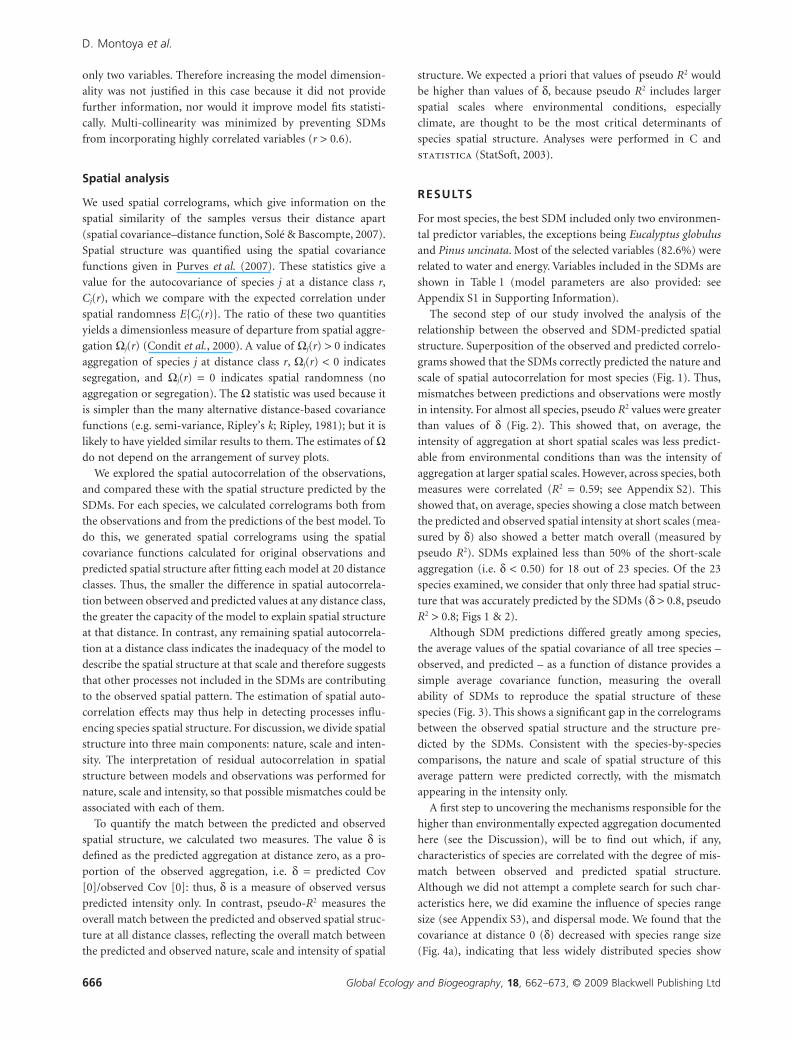
For most species, the best SDM included only two environmen-

tal predictor variables, the exceptions being Eucalyptus globulus

and Pinus uncinata. Most of the selected variables (82.6%) were

related to water and energy. Variables included in the SDMs are

shown in Table 1 (model parameters are also provided: see

Appendix S1 in Supporting Information).

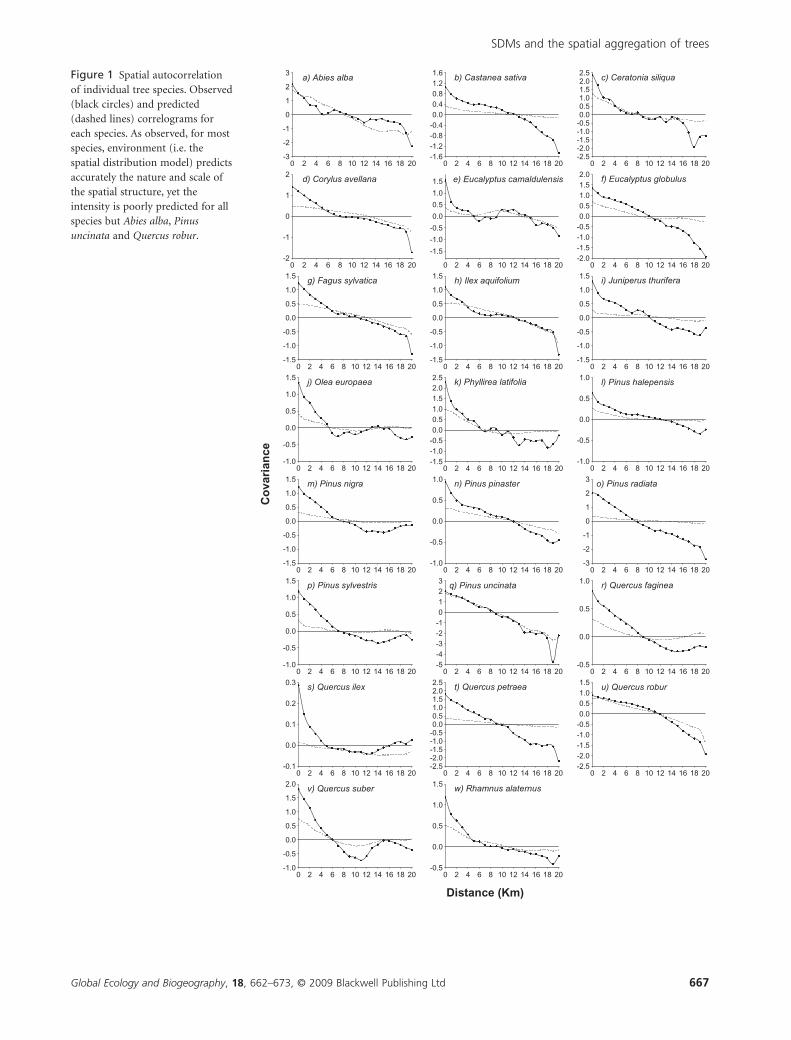
The second step of our study involved the analysis of the

relationship between the observed and SDM-predicted spatial

structure. Superposition of the observed and predicted correlo-

grams showed that the SDMs correctly predicted the nature and

scale of spatial autocorrelation for most species (Fig. 1). Thus,

mismatches between predictions and observations were mostly

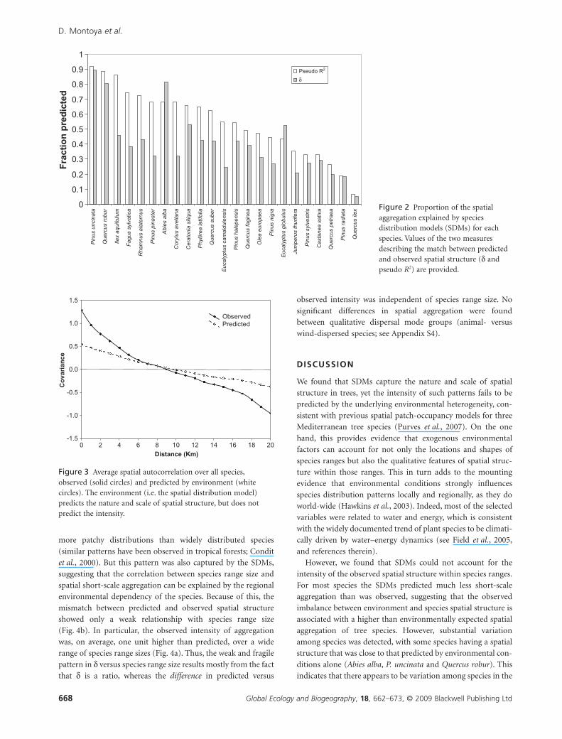
in intensity. For almost all species, pseudo R2 values were greater

than values of d (Fig. 2). This showed that, on average, the

intensity of aggregation at short spatial scales was less predict-

able from environmental conditions than was the intensity of

aggregation at larger spatial scales. However, across species, both

measures were correlated (R2 = 0.59; see Appendix S2). This

showed that, on average, species showing a close match between

the predicted and observed spatial intensity at short scales (mea-

sured by d) also showed a better match overall (measured by

pseudo R2). SDMs explained less than 50% of the short-scale

aggregation (i.e. d < 0.50) for 18 out of 23 species. Of the 23

species examined, we consider that only three had spatial struc-

ture that was accurately predicted by the SDMs (d > 0.8, pseudo

R2 > 0.8; Figs 1 & 2).

Although SDM predictions differed greatly among species,

the average values of the spatial covariance of all tree species –

observed, and predicted – as a function of distance provides a

simple average covariance function, measuring the overall

ability of SDMs to reproduce the spatial structure of these

species (Fig. 3). This shows a significant gap in the correlograms

between the observed spatial structure and the structure pre-

dicted by the SDMs. Consistent with the species-by-species

comparisons, the nature and scale of spatial structure of this

average pattern were predicted correctly, with the mismatch

appearing in the intensity only.

A first step to uncovering the mechanisms responsible for the

higher than environmentally expected aggregation documented

here (see the Discussion), will be to find out which, if any,

characteristics of species are correlated with the degree of mis-

match between observed and predicted spatial structure.

Although we did not attempt a complete search for such char-

acteristics here, we did examine the influence of species range

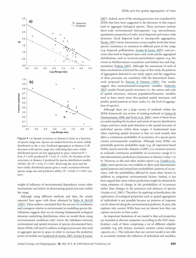
size (see Appendix S3), and dispersal mode. We found that the

covariance at distance 0 (d) decreased with species range size

(Fig. 4a), indicating that less widely distributed species show

D. Montoya et al.

Global Ecology and Biogeography, 18, 662–673, © 2009 Blackwell Publishing Ltd666

0 2 4 6 8 10 12 14 16 18 20-3

-2

-1

0

1

2

3a) Abies alba

0 2 4 6 8 10 12 14 16 18 20-1.6-1.2-0.8-0.40.00.40.81.21.6

b) Castanea sativa

0 2 4 6 8 10 12 14 16 18 20-2.5-2.0-1.5-1.0-0.50.00.51.01.52.02.5

c) Ceratonia siliqua

0 2 4 6 8 10 12 14 16 18 20-2

-1

0

1

2d) Corylus avellana

0 2 4 6 8 10 12 14 16 18 20

-1.5

-1.0

-0.5

0.0

0.5

1.0

1.5 e) Eucalyptus camaldulensis

0 2 4 6 8 10 12 14 16 18 20-2.0-1.5-1.0-0.50.00.51.01.52.0 f) Eucalyptus globulus

0 2 4 6 8 10 12 14 16 18 20-1.5

-1.0

-0.5

0.0

0.5

1.0

1.5 g) Fagus sylvatica

0 2 4 6 8 10 12 14 16 18 20-1.5

-1.0

-0.5

0.0

0.5

1.0

1.5 h) Ilex aquifolium

0 2 4 6 8 10 12 14 16 18 20-1.5

-1.0

-0.5

0.0

0.5

1.0

1.5 i) Juniperus thurifera

0 2 4 6 8 10 12 14 16 18 20-1.0

-0.5

0.0

0.5

1.0

1.5 j) Olea europaea

0 2 4 6 8 10 12 14 16 18 20-1.5-1.0-0.50.00.51.01.52.02.5 k) Phyllirea latifolia

0 2 4 6 8 10 12 14 16 18 20-1.0

-0.5

0.0

0.5

1.0 l) Pinus halepensis

0 2 4 6 8 10 12 14 16 18 20-1.5

-1.0

-0.5

0.0

0.5

1.0

1.5 m) Pinus nigra

0 2 4 6 8 10 12 14 16 18 20-1.0

-0.5

0.0

0.5

1.0 n) Pinus pinaster

0 2 4 6 8 10 12 14 16 18 20-3

-2

-1

0

1

2

3 o) Pinus radiata

0 2 4 6 8 10 12 14 16 18 20-1.0

-0.5

0.0

0.5

1.0

1.5 p) Pinus sylvestris

0 2 4 6 8 10 12 14 16 18 20-5-4-3-2-10123 q) Pinus uncinata

0 2 4 6 8 10 12 14 16 18 20-0.5

0.0

0.5

1.0 r) Quercus faginea

0 2 4 6 8 10 12 14 16 18 20-0.1

0.0

0.1

0.2

0.3 s) Quercus ilex

0 2 4 6 8 10 12 14 16 18 20-2.5-2.0-1.5-1.0-0.50.00.51.01.52.02.5 t) Quercus petraea

0 2 4 6 8 10 12 14 16 18 20-2.5-2.0-1.5-1.0-0.50.00.51.01.5 u) Quercus robur

Co

vari

ance

0 2 4 6 8 10 12 14 16 18 20-1.0

-0.5

0.0

0.5

1.0

1.5

2.0 v) Quercus suber

0 2 4 6 8 10 12 14 16 18 20-0.5

0.0

0.5

1.0

1.5 w) Rhamnus alaternus

Distance (Km)

Figure 1 Spatial autocorrelationof individual tree species. Observed(black circles) and predicted(dashed lines) correlograms foreach species. As observed, for mostspecies, environment (i.e. thespatial distribution model) predictsaccurately the nature and scale ofthe spatial structure, yet theintensity is poorly predicted for allspecies but Abies alba, Pinusuncinata and Quercus robur.

SDMs and the spatial aggregation of trees

Global Ecology and Biogeography, 18, 662–673, © 2009 Blackwell Publishing Ltd 667

more patchy distributions than widely distributed species

(similar patterns have been observed in tropical forests; Condit

et al., 2000). But this pattern was also captured by the SDMs,

suggesting that the correlation between species range size and

spatial short-scale aggregation can be explained by the regional

environmental dependency of the species. Because of this, the

mismatch between predicted and observed spatial structure

showed only a weak relationship with species range size

(Fig. 4b). In particular, the observed intensity of aggregation

was, on average, one unit higher than predicted, over a wide

range of species range sizes (Fig. 4a). Thus, the weak and fragile

pattern in d versus species range size results mostly from the fact

that d is a ratio, whereas the difference in predicted versus

observed intensity was independent of species range size. No

significant differences in spatial aggregation were found

between qualitative dispersal mode groups (animal- versus

wind-dispersed species; see Appendix S4).

DISCUSSION

We found that SDMs capture the nature and scale of spatial

structure in trees, yet the intensity of such patterns fails to be

predicted by the underlying environmental heterogeneity, con-

sistent with previous spatial patch-occupancy models for three

Mediterranean tree species (Purves et al., 2007). On the one

hand, this provides evidence that exogenous environmental

factors can account for not only the locations and shapes of

species ranges but also the qualitative features of spatial struc-

ture within those ranges. This in turn adds to the mounting

evidence that environmental conditions strongly influences

species distribution patterns locally and regionally, as they do

world-wide (Hawkins et al., 2003). Indeed, most of the selected

variables were related to water and energy, which is consistent

with the widely documented trend of plant species to be climati-

cally driven by water–energy dynamics (see Field et al., 2005,

and references therein).

However, we found that SDMs could not account for the

intensity of the observed spatial structure within species ranges.

For most species the SDMs predicted much less short-scale

aggregation than was observed, suggesting that the observed

imbalance between environment and species spatial structure is

associated with a higher than environmentally expected spatial

aggregation of tree species. However, substantial variation

among species was detected, with some species having a spatial

structure that was close to that predicted by environmental con-

ditions alone (Abies alba, P. uncinata and Quercus robur). This

indicates that there appears to be variation among species in the

0

0.1

0.2

0.3

0.4

0.5

0.6

0.7

0.8

0.9

1

Pin

us u

ncin

ata

Que

rcus

rob

ur

Ilex

aqui

foliu

m

Fag

us s

ylva

tica

Rha

mnu

s al

ater

nus

Pin

us p

inas

ter

Abi

es a

lba

Cor

ylus

ave

llana

Cer

aton

ia s

iliqu

a

Phy

llire

a la

tifol

ia

Que

rcus

sub

er

Euc

alyp

tus

cam

aldu

lens

is

Pin

us h

alep

ensi

s

Que

rcus

fagi

nea

Ole

a eu

ropa

ea

Pin

us n

igra

Euc

alyp

tus

glob

ulus

Juni

peru

s th

urife

ra

Pin

us s

ylve

stris

Cas

tane

a sa

tiva

Que

rcus

pet

raea

Pin

us r

adia

ta

Que

rcus

ilex

Fra

ctio

n p

red

icte

dPseudo R2

δ

Figure 2 Proportion of the spatialaggregation explained by speciesdistribution models (SDMs) for eachspecies. Values of the two measuresdescribing the match between predictedand observed spatial structure (d andpseudo R2) are provided.

0 2 4 6 8 10 12 14 16 18 20Distance (Km)

-1.5

-1.0

-0.5

0.0

0.5

1.0

1.5

Co

vari

ance

Observed Predicted

Figure 3 Average spatial autocorrelation over all species,observed (solid circles) and predicted by environment (whitecircles). The environment (i.e. the spatial distribution model)predicts the nature and scale of spatial structure, but does notpredict the intensity.

D. Montoya et al.

Global Ecology and Biogeography, 18, 662–673, © 2009 Blackwell Publishing Ltd668

weight of influence of environmental dependency versus other

mechanisms (see below) in determining spatial structure within

the range.

Although using different methods and data, the results

reported here agree with those obtained by Bahn & McGill

(2007). These authors concluded that ‘the success of coordinates

and contagion relative to environment in modelling species dis-

tributions suggests that we are missing fundamental ecological

elements underlying distributions when we model them using

environmental conditions only’. Given the imbalance between

environment and spatial structure of species documented here,

future SDMs will need to address ecological processes that tend

to aggregate species in space in order to increase the predictive

power of models (see Leathwick & Austin, 2001; Araújo & Luoto,

2007). Indeed, most of the missing processes not considered by

SDMs that have been suggested in the literature in this respect

tend to aggregate biological species. These processes include

short-scale environmental heterogeneity (e.g. microclimates,

quantitative properties of soils), local dispersal and source–sink

dynamics (local dispersal leads to intraspecific aggregation;

Pacala, 1997); biotic interactions across trophic levels that foster

species coexistence or exclusion in different parts of the range

(e.g. dispersal, pollinization; Araújo & Luoto, 2007); and pro-

cesses that tend to fragment space and create patchy aggregated

distributions, such as recurrent perturbation regimes (e.g. fire

events in Mediterranean ecosystems) and habitat loss and frag-

mentation (Fahrig, 2003). Although the assessment of each of

these mechanisms is beyond the scope of this study, the patterns

of aggregation detected in our study region and the suggestion

of these processes are consistent with the hierarchical frame-

work proposed by Pearson & Dawson (2003). Our results

suggest that environmental/scenopoetic variables (Soberón,

2007) predict broad spatial structures (i.e. the nature and scale

of spatial structure), whereas population/bionomic variables

tend to have much more fine-grained spatial structures and

predict spatial patterns at lower scales (i.e. the level of aggrega-

tion of species).

Although there are a large variety of methods within the

SDMs framework (see review of existing methods in Guisan &

Zimmermann, 2000, and Scott et al., 2002), most of them focus

on understanding the location and extent of species distribution

ranges and have rarely paid attention to the spatial structure of

individual species within these ranges. A fundamental issue

when exploring spatial structure is that we need models that

allow a continuous probability of occurrence of a species given

certain environmental conditions. Although most SDMs can

potentially generate probability maps (e.g. all regression-based

SDMs, neural networks, Maxent, GARP), it is common practice

to reclassify continuous probability of occurrence (range 0–1)

into deterministic predictions of presence or absence (value 1 or

0). However, as this and other studies report (e.g. Condit et al.,

2000), most species are very unlikely to show such deterministic

spatial patterns and instead have probabilistic patterns of occur-

rence, with the probabilities affected by many other factors in

addition to exogenous environmental factors. Indeed, it has

been argued that more robust predictions might be obtained by

using estimates of change in the probabilities of occurrence

rather than changes in the presences and absences of species

(Araújo et al., 2005). Therefore, by applying reclassification, the

exploration of ecological properties such as spatial aggregation

of individuals is not possible because no patterns of response

can be observed along the environmental gradients. In part, this

explains why current SDMs have not yet shown how they can

capture structure at finer scales.

An important limitation of our model is that soil properties

are included as discrete categories (according to the FAO classi-

fication), each of them comprising a set of different edaphic

variables (e.g. pH, texture, moisture content, cation exchange

capacity, etc.). This indicates that our current model is not able

to accurately estimate the influence of individual soil variables,

-3.5 -3.0 -2.5 -2.0 -1.5 -1.0 -0.5 0.0

Log (Range size)

0.0

0.5

1.0

1.5

2.0

2.5

3.0

3.5d

Observed Predicted

a)

-3.5 -3.0 -2.5 -2.0 -1.5 -1.0 -0.5 0.0

Log (Range size)

0.0

0.1

0.2

0.3

0.4

0.5

0.6

0.7

0.8

0.9

1.0

Fra

ctio

n p

red

icte

d

b)

Figure 4 (a) Spatial covariance at distance 0 (km) as a functionof species range size. Species are ranked from less to more widelydistributed on the x-axis. Predicted aggregation at distance 0 (d)decreases with species range size, indicating that more widelydistributed species are less aggregated in space (observed R2 =0.64, P < 0.05; predicted R2 = 0.62, P < 0.05). (b) Fraction of thecovariance at distance 0 predicted by species distribution models(SDMs) (d) (R2 = 0.26, P < 0.05). Removing the most and theleast widely distributed species gives a weak correlation betweenspecies range size and predictive ability (R2 = 0.026, P < 0.05) (seetext).

SDMs and the spatial aggregation of trees

Global Ecology and Biogeography, 18, 662–673, © 2009 Blackwell Publishing Ltd 669

leaving open the possibility that some of the unexplained varia-

tion in the intensity of spatial structure is due to species

responses to variation in soil. If so, this would not just be a case

of an important exogenous environmental factor that has been

missed. Rather, unlike most of the factors considered here, soil is

heavily affected by the presence or absence of the species, over

and above those aspects of soil that are defined exogenously (e.g.

bedrock types). Because soil may determine the spatial structure

of biological communities (Coudun et al., 2006), especially for

those species that are more substrate dependent, it would be

beneficial if future SDMs included high-resolution soil datasets

at large scales.

A potential problem with the model presented here is that it

assumes normal (Gaussian) responses between species occur-

rence and environmental variables. This is a common assump-

tion in niche theory and SDMs (Austin, 2002) also made by our

model. The functional response of species to environmental

gradients is still a matter of debate: for example, it has been

argued that symmetric unimodal responses are rare whereas

skewed curves predominate (see Austin, 2002). On the other

hand, the real response curves of species to environmental vari-

ables can be quantified only when all other factors are non-

limiting, an unlikely phenomenon in nature (Huston, 2002). It

remains to be seen whether SDMs with alternative functional

forms might reproduce spatial structure more accurately than

those documented here: although the observed deviation in this

case was so large (Fig. 1) that it seems unlikely that the mis-

matches can be attributed entirely, or even mainly, to this

problem.

Another common and necessary assumption in large-scale

distribution modelling is that tree populations are in pseudo-

equilibrium with environmental conditions (Guisan & Zimmer-

mann, 2000; Pearson & Dawson, 2003). However, the validity of

this assumption varies across different groups of organisms, and

among species within the same group (Araújo & Pearson, 2005).

This is the case for exotic species. Whereas some of the exotic

species in the Iberian Peninsula have been naturalized over time

since their first introduction (e.g. Castanea sativa), others (e.g.

Pinus radiata and Eucalyptus sp.) have been recently introduced

as plantations. The time for naturalization for these species has

been very short as most plantations were planted primarily in

the second half of the 20th century (Blondel & Aronson, 1999).

This suggests that spatial distributions associated with recently

introduced species do not fit with the pseudo-equilibrium

assumption between species occurrence and environmental

conditions. Indeed, in this case spatial structure is poorly

explained by environmental conditions for most exotic trees,

especially P. radiata (see Fig. 2). This raises the possibility that,

in other cases, a mismatch between predicted and observed fine-

scale spatial structure might be a useful indicator of non-

equilibrium. Results for introduced tree species should thus be

taken cautiously because they may be reflecting their allochtho-

nous nature.

Given the reported time lags in the recolonization of northern

latitudes following Holocene warming in Europe (Svenning &

Skov, 2004; Araújo & Pearson, 2005), the equilibrium between

species distributions and environmental conditions may be

associated with the distance to historical glacial refugia. Indeed,

major biological regions in Europe are determined more by the

location of these glacial refugia than by current climate gradi-

ents (Araújo & Pearson, 2005; Svenning & Skov, 2005, 2007).

Because the last glacial episode affected more intensely the areas

historically covered by ice than the southern ice-free regions of

Europe (Montoya et al., 2007), and the Iberian Peninsula is

located in a historical glacial refugium where trees were not

excluded (Hewitt, 2000; Carrión et al., 2003), it is reasonable to

consider that tree species in continental Spain are closer to equi-

librium than tree species living in northern areas (except exotic

species), simply because species have had more time and less

dispersal distance to colonize suitable areas. The equilibrium

assumption also depends on the dispersal abilities of individual

species to colonize environmentally suitable regions (Tyre et al.,

2001). For example, animal dispersal of seeds is generally

addressed to longer distances than wind dispersal. Fourteen out

of our 23 tree species are dispersed by animals, which suggests

that, given enough time, at least these species might be at equi-

librium with the environment. However, previous studies have

shown that the response of certain individual trees to glacial

history indicates strong links between the location of glacial

refugia and spatial patterns of trees in the Iberian Peninsula

(Benito Garzón et al., 2007). Therefore, a reasonable conclusion

is that whereas spatial restrictions apply to a subset of species,

others might be at equilibrium with current environmental con-

ditions in our study region.

Finally, the equilibrium assumption is less apparent in dis-

turbed ecosystems such as Mediterranean forests, where human

influence is strong. In this case, the observed imbalance between

environment and spatial aggregation of tree species might be

explained by the lack of equilibrium between species and

current environmental conditions. However, because attempts

to incorporate population-level processes such as biotic interac-

tions into the SDM framework (Leathwick & Austin, 2001;

Araújo & Luoto, 2007) have shown that combined population–

environmental models have more predictive power than pure

environmental models, it is reasonable to conclude that

population-level processes explain at least part of the difference

in spatial aggregation of tree species between SDMs and obser-

vations. Despite this, it is important to bear in mind that our

results are restricted to tree species in continental Spain, and

thus we are not certain to what extent any patterns or results that

we observe here may be extrapolated to other regions.

Patchiness, or the degree to which individuals are aggregated,

is crucial for understanding the dynamics of forest communi-

ties, such as how a given species uses resources and is used as a

resource, and to describe the species’ reproductive biology.

Information on spatial aggregation of a species can be also criti-

cal for predicting its distribution in a different region or future

distributions following landscape changes (e.g. climate change).

Moreover, the aim of reserve design is to select a small but

efficient network of sites for conservation. In such a case, robust

prediction of the distribution and spatial structure of the species

in the selected network is crucial (Araújo & Williams, 2000;

D. Montoya et al.

Global Ecology and Biogeography, 18, 662–673, © 2009 Blackwell Publishing Ltd670

Araújo et al., 2002). However, given the high variation in the

accuracy of SDM predictions (Segurado & Araújo, 2004;

Pearson et al., 2006) and the species-specific nature of biological

responses to landscape changes (e.g. climate change; Kerr &

Kharouba, 2007), it seems clear that predicting the responses of

individual species will often be difficult. A promising avenue is

that recent studies suggest that species traits are behind these

interspecific differences, and that species might therefore be

aggregated into functional groups according to physiological

and demographic traits. For example, Pöyry et al. (2008) have

shown that the quality of SDMs for a set of 98 species of but-

terflies is shaped by processes operating at the population level.

These authors found that the spatial distribution of species with

low mobility and short flight periods was modelled more accu-

rately than that of species with high mobility and long flight

periods. Future studies should address empirically the question

of which traits reduce the uncertainty associated with environ-

mental models, and identify relevant traits to understand the

spatial distributions of species under global change.

In summary, although SDMs are a general and widely used

approximation to modelling species distributions, future con-

servation strategies will require models that incorporate greater

biological realism (Hampe, 2004; Keith et al., 2008). Spatial

structure analyses within species distribution ranges show that

SDMs capture very accurately the nature and scale of the spatial

structure of tree species, yet the intensity or level of aggregation

of species in space is captured poorly. Species are more aggre-

gated in space than environmentally expected, and so the devel-

opment of more realistic SDMs should focus on those ecological

processes that increase species aggregation.

ACKNOWLEDGEMENTS

We thank the Ministerio de Medio Ambiente, Spain, and

R. Vallejo and J. A. Villanueva for help with IFN2 data. We

also thank M. A. Rodríguez for his useful comments on first

versions of the manuscript, and three anonymous referees

for their comments and suggestions. D.M. was supported by

the Spanish Ministry for Education and Science (fellowship

AP2004-0075). M.A.Z. was supported by the DINAMED project

(grant CGL2005-05830-03), and INTERBOS3 project (grant

CDL2008-04503-03-03). This research is part of the GLO-

BIMED (http://www.globimed.net/) network of forest ecology.

REFERENCES

Anderson, R.A., Peterson, A.T. & Gómez-Laverde, M. (2002)

Using niche-based GIS modelling to test geographic predic-

tions of competitive exclusion and competitive release in

South American pocket mice. Oikos, 98, 3–16.

Araújo, M.B. & Luoto, M. (2007) The importance of biotic

interactions for modelling species distributions under climate

change. Global Ecology and Biogeography, 16, 743–753.

Araújo, M.B. & Pearson, R.G. (2005) Equilibrium of species’

distributions with climate. Ecography. 28, 693–695.

Araújo, M.B. & Williams, P.H. (2000) Selecting areas for species

persistence using occurrence data. Biological Conservation, 96,

331–345.

Araújo, M.B., Williams, P.H. & Turner, A. (2002) A sequential

approach to minimize threats within selected conservation

areas. Biodiversity and Conservation, 11, 1011–1024.

Araújo, M.B., Whittaker, R.J., Ladle, R.J. & Erhard, M. (2005)

Reducing uncertainty in projections of extinction risk

from climate change. Global Ecology and Biogeography, 14,

529–538.

Austin, M.P. (2002) Spatial prediction of species distribution: an

interface between ecological theory and statistical modelling.

Ecological Modelling, 157, 101–118.

Bahn, V. & McGill, B.J. (2007) Can niche-based distribution

models outperform spatial interpolation? Global Ecology and

Biogeography, 16, 733–742.

Benito Garzón, M., Sánchez de Dios, R. & Sáinz Ollero, H.

(2007) Predictive modelling of tree species distributions on

the Iberian Peninsula during the Last Glacial Maximum and

Mid-Holocene. Ecography, 30, 120–134.

Blondel, J. & Aronson, J.C. (1999) Biology and wildlife of the

Mediterranean region. Oxford University Press, Oxford.

Carrión, J.S., Yll, E.I., Walker, M.J., Legaz, A.J., Chaín, C. &

López, A. (2003) Glacial refugia of temperate, Mediterranean

and Ibero-North African flora in south-eastern Spain: new

evidence from cave pollen at two Neanderthal sites. Global

Ecology and Biogeography, 12, 119–129.

Condit, R., Ashton, P.S., Baker, P., Bunyavejchewin, S.,

Gunatilleke, S., Gunatilleke, N., Hubbell, S.P., Foster, R.B.,

Itoh, A., LaFrankie, J.V., Lee, H.S., Losos, E., Manokaran, N.,

Sukumar, R. & Yamakura, T. (2000) Spatial patterns in the

distribution of tropical tree species. Science, 288, 1414–1418.

Coudun, C., Gégout, J.-C., Piedallu, C. & Rameau, J.-C. (2006)

Soil nutritional factors improve models of plant species dis-

tribution: an illustration with Acer campestre (L.) in France.

Journal of Biogeography, 33, 1750–1763.

FAO (1988) Soil map of the world. FAO/UNESCO, Rome.

Available at: http://www.fao.org/AG/agl/agll/dsmw.htm (last

accessed August 2008).

Fahrig, L. (2003) Effects of habitat fragmentation on biodiver-

sity. Annual Review of Ecology and Systematics, 34, 487–515.

Field, R., O’Brien, E.M. & Whittaker, R.J. (2005) Global models

for predicting woody plant richness from climate: develop-

ment and evaluation. Ecology, 86, 2263–2277.

Guisan, A. & Zimmermann, N.E. (2000) Predictive habitat dis-

tribution models in ecology. Ecological Modelling, 135, 147–

186.

Gutiérrez, D., Fernández, P., Seymour, A.S. & Jordano, D. (2005)

Habitat distribution models: are mutualist distributions good

predictors of their associates? Ecological Applications, 15, 3–18.

Hampe, A. (2004) Bioclimate envelope models: what they detect

and what they hide. Global Ecology and Biogeography, 13, 469–

476.

Hawkins, B.A., Field, R., Cornell, H.V., Currie, D.J., Guégan, J.-F.,

Kaufman, D.M., Kerr, J.T., Mittelbach, G.G., Oberdorff, T.,

O’Brien, E.M., Porter, E.E. & Turner, J.R.G. (2003) Energy,

SDMs and the spatial aggregation of trees

Global Ecology and Biogeography, 18, 662–673, © 2009 Blackwell Publishing Ltd 671

water, and broad-scale geographic patterns of species rich-

ness. Ecology, 84, 3105–3117.

Hewitt, G.M. (2000) The genetic legacy of the Quaternary ice

ages. Nature, 405, 907–913.

Hilborn, R. & Mangel, M. (1997) The ecological detective. Con-

fronting models with data. Monographs in population biology

28. Princeton University Press, Princeton, NJ.

Huntley, B., Berry, P.M., Cramer, W. & McDonald, A.P. (1995)

Modelling present and potential future ranges of some Euro-

pean higher plants using climate response surfaces. Journal of

Biogeography, 22, 967–1001.

Huston, M.A. (2002) Introductory essay: critical issues for

improving predictions. Predicting species occurrences: issues of

scale and accuracy (ed. by J.M. Scott, P.J. Heglund, M.L.

Morrison, J.B. Haufler, M.G. Raphael, W.A. Wall and F.B.

Samson), pp. 7–21. Island Press, Washington, DC.

Inventario Forestal Nacional. (1995) Segundo inventario forestal

nacional. Ministerio de Agricultura, Pesca y Alimentación,

Madrid, Spain.

Jensen, M.E. & Haise, H.R. (1963) Estimating evapotranspira-

tion from solar radiation. Journal of Irrigation and Drainage

Engineering ASCE, 89, 15–41.

Keith, D.A., Akçakaya, H.R., Thuiller, W., Midgley, G.F., Pearson,

R.G., Phillips, S.J., Regan, H.M., Araújo, M.B. & Rebelo, T.G.

(2008) Predicting extinction risks under climate change: cou-

pling stochastic population models with dynamic bioclimatic

habitat models. Biology Letters, 4, 560–563.

Kerr, J.T. & Kharouba, H. (2007) Climate change and conserva-

tion. Theoretical ecology (ed. by R. May and A. McLean), pp.

190–204. Oxford University Press, Oxford.

Leathwick, J.R. & Austin, M.P. (2001) Competitive interactions

between tree species in New Zealand’s old growth indigenous

forests. Ecology, 82, 2560–2573.

Lehman, C.L. & Tilman, D. (1997) Competition in spatial habi-

tats. Spatial ecology: the role of space in population dynamics

and interspecific interactions (ed. by D. Tilman and P. Kareiva),

pp. 185–203. Princeton University Press, Princeton, NJ.

Metropolis, N., Rosenbluth, A.W., Rosenbluth, M.N., Teller,

A.H. & Teller, E. (1953) Equations of state calculations by fast

computing machines. Journal of Chemical Physics, 21, 1087–

1092.

Montoya, D., Rodríguez, M.A., Zavala, M.A. & Hawkins, B.A.

(2007) Contemporary richness of Holarctic trees and the his-

torical pattern of glacial retreat. Ecography, 30, 173–182.

Ninyerola, M., Pons, X. & Roure, J.M. (2005) Atlas climático

digital de la Península Ibérica. Metodología y aplicaciones en

bioclimatología y geobotánica, Universidad Autónoma de Bar-

celona, Bellaterra. Available at: http://www.opengis.uab.es/

wms/iberia/index.htm (last accessed June 2008).

Pacala, S.W. (1997) Dynamics of plant communities. Plant

ecology (ed. by M.J. Crawley), pp. 532–555. Blackwell Scien-

tific Publications, Oxford.

Pearson, R.G. & Dawson, T.P. (2003) Predicting the impacts of

climate change on the distribution of species: are bioclimate

envelope models useful? Global Ecology and Biogeography, 12,

361–371.

Pearson, R.G., Thuiller, W., Araújo, M.B., Martínez-Meyer, E.,

Brotons, L., McClean, C., Miles, L., Segurado, P., Dawson, T.P.

& Lees, D.C. (2006) Model-based uncertainty in species

range prediction. Global Ecology and Biogeography, 33, 1704–

1711.

Peterson, A.T., Ortega-Huerta, M.A., Bartley, J., Sánchez-

Cordero, V., Soberón, J., Buddemeier, R.H. & Stockwell, D.R.

(2002) Future projections for Mexican faunas under global

climate change scenarios. Nature, 416, 626–629.

Pöyry, J., Luoto, M., Heikkinen, R.K. & Saarinen, K. (2008)

Species traits are associated with the quality of bioclimatic

models. Global Ecology and Biogeography, 17, 403–414.

Purves, D.W., Zavala, M.A., Ogle, K., Prieto, F. & Rey Benayas,

J.M. (2007) Environmental heterogeneity, bird-mediated

directed dispersal, and oak woodland dynamics in Mediterra-

nean Spain. Ecological Monographs, 77, 77–97.

Ripley, B.D. (1981) Spatial statistics. John Wiley and Sons, New

York.

Scott, J.M., Heglund, P.J., Haufler, J.B., Morrison, M., Raphael,

M.G. & Wall, W.B. (2002) Predicting species occurrences: issues

of accuracy and scale. Island Press, Covelo, CA.

Segurado, P. & Araújo, M. (2004) An evaluation of methods for

modelling species distributions. Journal of Biogeography, 31,

1555–1569.

Soberón, J. (2007) Grinnellian and Eltonian niches and geo-

graphic distributions of species. Ecology Letters, 10, 1115–

1123.

Solé, R.V. & Bascompte, J. (2007) Self-organization in complex

ecosystems. Princeton University Press, Princeton, NJ.

StatSoft, Inc. (2003) STATISTICA (data analysis software

system), Version 6. Available at http://www.statsoft.com (last

accessed August 2008).

Svenning, J.-C. & Skov, F. (2004) Limited filling of the potential

range in European tree species. Ecology Letters, 7, 565–573.

Svenning, J.-C. & Skov, F. (2005) The relative roles of environ-

ment and history as controls of tree species composition

and richness in Europe. Journal of Biogeography, 32, 1019–

1033.

Svenning, J.-C. & Skov, F. (2007) Could the tree diversity pattern

in Europe be generated by postglacial dispersal limitation?

Ecology Letters, 10, 453–460.

Thomas, C.D., Cameron, A., Green, R.E., Bakkenes, M.,

Beaumont, L.J., Collingham, Y.C., Erasmus, B.F., De Siqueira,

M.F., Grainger, A., Hannah, L., Hughes, L., Huntley, B., Van

Jaarsveld, A.S., Midgley, G.F., Miles, L., Ortega-Huerta, M.A.,

Peterson, A.T., Phillips, O.L. & Williams, S.E. (2004) Extinc-

tion risk from climate change. Nature, 427, 145–148.

Thornthwaite, C.W. (1948) An approach toward a rational clas-

sification of climate. Geographical Review, 38, 55–94.

Thornthwaite, C.W. (1957) Instructions and tables for computing

potential evapotranspiration and the water balances. Labora-

tory of Climatology, Centerton, NJ.

Thuiller, W., Lavorel, S., Araújo, M.B., Sykes, M.T. & Prentice,

I.C. (2005) Climate change threats plant diversity in Europe.

Proceedings of the National Academy of Sciences USA, 102,

8245–8250.

D. Montoya et al.

Global Ecology and Biogeography, 18, 662–673, © 2009 Blackwell Publishing Ltd672

Tyre, A.J., Possingham, H.P. & Lindenmayer, D.B. (2001) Match-

ing observed pattern with ecological process: can territory

occupancy provide information about life history parameters?

Ecological Applications, 11, 1722–1738.

SUPPORTING INFORMATION

Additional Supporting Information may be found in the online

version of this article:

Appendix S1 Maximum likelihood estimates (MLE) for each

species-specific model.

Appendix S2 Relationship between predicted aggregation at

distance 0 (d) and overall predicted spatial structure (pseudo

R2).

Appendix S3 Relationship between species range size and

overall predicted spatial structure (pseudo R2).

Appendix S4 Permutation test on the relationship between

spatial aggregation and qualitative dispersal mode.

As a service to our authors and readers, this journal provides

supporting information supplied by the authors. Such materials

are peer-reviewed and may be re-organized for online delivery,

but are not copy-edited or typeset. Technical support issues

arising from supporting information (other than missing files)

should be addressed to the authors.

BIOSKETCHES

Daniel Montoya is a PhD student at the University of

Alcalá, Spain. His main research combines theoretical,

computational and empirical data to study how spatial

processes affect biodiversity patterns from local to

continental scales. He is especially interested in the

effects of perturbations, such as habitat loss and global

change, on ecological networks and distribution

patterns of species.

Editor: José Alexandre F. Diniz-Filho.

SDMs and the spatial aggregation of trees

Global Ecology and Biogeography, 18, 662–673, © 2009 Blackwell Publishing Ltd 673