1

Does Inequality Hinder the Diffusion of Technology? Preliminary Explorations By

Pedro Conceição, Pedro Faria, Pedro Ferreira, Beatriz Padilla, and Miguel T. Preto

IN+ Center for Innovation, Technology and Policy Research Instituto Superior Técnico, Lisbon, Portugal

Abstract This paper presents preliminary results of empirical tests of the hypothesis that inequality hinders the diffusion of new technologies.. Rather than considering the skill-biased technological change (which looks at how new production technologies require skills that are complementary to them, and lead to a rising premium for these skills that may result in growing inequality), we suggest to test whether inequality levels may limit the ability of individuals to acquire new consumption technologies. This hypothesis predicts a negative effect of inequality on the rate of diffusion of new technologies (we consider here the diffusion of three information and communications technologies). The preliminary results suggest that the effect of inequality on technology diffusion is positive. While this may indicate that our hypothesis should be rejected, a number of aspects suggest that this result should not be considered final until further explorations are undertaken. 1. Introduction The relationship between economic inequality and technology is traditionally conceptualized as one-way: new technologies are understood to contribute to the increase of economic inequality. The rationale for this understanding is based on the hypothesis that technological change is skill biased. New technologies create the demand for new skills, which are in low supply at the moment when the new technologies begin to diffuse. As the technology diffuses, the demand for these (new) skills increases, and since supply is tight those with the skills in demand see their wages increase, while other skills are remunerated at the same rate as before. The recent increase in economic inequality in most developed countries has been attributed to the diffusion of information technology, especially computers, raising the wage premium for computer programmers and, in general, computer literate people (see, for example, Acemoglu 2002a). The skill-biased technological-change hypothesis is based on the assumption that there is a complementarity between skills and new technologies. Several models have provided a formal way to interpret this hypothesis, including Krussell et al (1997), Vindigni (2002), Acemoglu and Pieshcke (2000) and Card and Lemieux (2000), Bound & Johnson (1992), Schmitt (1995)1. Caselli´s (1999) approach is more flexible and sophisticated, since instead of focusing on the substitutability between skilled and unskilled labor or skill-complementary technology, he focused on substitutability among technologies, where technological change is produced by substitution between types of capital. Technological change can be skill biased (if new skills are more expensive to acquire than the skills required by pre-existing technologies, i.e. information technologies) or de-skilling (if the new skills can be acquired at a lower cost than the pre-existing technologies, i.e. assembly line). Aghion and Williamson (1998), while acknowledging that the drivers of inequality are little understood, still argue that one of the factors that pushed income inequality up has been technological change. Other researchers have focused on alternative explanations for the increase in inequality. Acemoglu (2002b) compares changes in the wage structure in the United States, the United Kingdom and Continental Europe. While he agrees with the fact that wage inequality rose because the demand for high skilled workers increased relative to their supply, he raises the question of why the process has been different in Europe. He offers three explanations. One is that relative supply of skills increased faster in Europe accounting for less increased in inequality. Second, the European wage institutions (such as unions) have helped to prevent rising inequalities. The third explanation, non-traditional, suggests that technical change has been less skill biased in Europe, maybe due to different explanatory factors: countries develop their own technologies which are less

1 In some models the increase in skill-premium in also linked to an increased to the premium of higher educational levels. In some models, credit constraints explain why inequality persists: the less-skilled not only earn lower salaries, but lack the income to invest in education that would provide them with the skills allowing them to “jump” to higher wage levels.

2

skill-biased or that those countries may lag behind the world technology frontier having different incentives to adopt new technologies. In this sense, and due to wage compression in Europe, firms may find more profitable to adopt new technologies that fit more unskilled workers. Consequently, job creation is less profitable in Europe and in the long run, it manifests in the increase of unemployment. In terms of empirical work, Krueger (1993) found evidence that employees that directly use computers at work earn higher salaries. Because highly educated workers are more likely to use computers on the job, the proliferation of computers (technological change) explains, according to this author, the increasing returns to education between 1984 and 1989. Autor et al (1997) explore this issue finding that the diffusion of computers explains 40% of the changes in wages toward college graduates, while investments in computers accounts for at least 30% in the increase in the rate of within-industry skill upgrading. Challenging these findings, DiNardo and Pischke (1997) believe that the causal effects of computer use on wages are not so straightforward. Applying similar statistical techniques to those used by Krueger, they illustrate that the wage differentials associated with the use of calculators, a telephone, a pen or a pencil, or even sitting on the job, are very similar to those measured by computer use. Instead, their results suggest that computer users have unobserved skills which may have little to do with the use of computers but that are rewarded in labor markets, or that computers were introduced in jobs that were already of higher wages. Borghans and ter Weel (2002) take a different approach. They start from the observation that computer use increases individual productivity as well as the supply of goods. They argue that the maximum level of wage inequality depends on the distribution of productivity of workers within and between groups. In the initial phase, wage inequality tends to increase. In the long run, wage inequality tends to decrease depending on the productivity gains from using computers. These authors also explore a related issue. They wonder if computer skills are really needed to use a computer. They conclude that computer skills in general do not yield significant labor market returns, unless we refer to the highest level of sophistication in the use of computers, which is not widespread. Acemoglu and Zilibotti (2001) are concerned with differences in productivity between the developed and developing countries. The differences arise because most technologies adopted by developing countries are developed in the industrialized countries and thus are designed to make optimal use of the skilled labor force. In less developed countries, the workforce is less skilled, and so less productive in the use of those technologies. The obvious consequence is that even if all countries have equal access to new technologies, the mismatch between skills and technologies leads to differences in total factor productivity. Other problems associated with less developed countries are: the specialization of the South in low skilled tasks, and the lack of poor intellectual property rights enforcement. In response to these issues they suggest that protecting property rights and educating the labor force would lead to convergence and income and productivity inequalities would stabilize. As exposed above, the literature on wage inequality and technological change is vast. However, the perspectives taken tend to follow the skill-biased technological change hypothesis, with modeling and empirical variation on the same theme. The relationship between inequality and diffusion is taken from the perspective of the production side of the economy. The issue of how inequality influences the adoption of technologies of consumption is seldom studied and there is a clear lack of empirical models and data to illustrate it. The question is also rarely analyzed at the level of cross-country comparisons and the, possibly, more complex relationship between technological change and inequality is not commonly acknowledged. Still, as we will briefly describe below, there are exceptions. Sachs (2002) in a recent speech talked about the global innovation divide and characterized poor countries as “the excluded poor” and suggesting that the international community should support their science and technology needs by doing something about those countries trapped by extreme poverty, geographical isolation and ecological distress. Similarly, Castells (1998) identified the fourth world, as those countries that are pretty much excluded from the ICT revolution. In many different aspects, he is concerned with what has been named “the information age”. Castells believes that an escape from this fourth world (the excluded poor for Sachs) is possible, but it would require massive technological upgrading of countries, firms and households, upgrading of the educational system, establishing a world wide network of science and technology and reversing the marginalization of entire countries, cities or neighborhoods.

3

Pippa Norris (2001) is preoccupied with the root causes and the consequences of the inequalities that characterized the first decade of the diffusion of the Internet. In relation to inequality or the digital divide as a multidimensional phenomenon, she considers three different aspects: the global divide or divergence of Internet access between developing and industrialized countries, the social divide or the gap between information rich and poor in each country, and the democratic divide, which is the difference between those who use and do not use digital resources to engage in public life. Her interest in inequalities deals with relative inequalities and whether there are special barriers to using digital technologies and if a technology such as the Internet has similar disparities in the penetration of older communication technologies. Hargittai (1999) looks at Internet connectivity differences across OECD countries, suggesting that even among these “more similar countries”, it is possible to find differences in relation to Internet connectivity. This study indicates that there are several factors that influence the process of diffusion, among them economic indicators, human capital, the institutional legal environment, and the existing technological infrastructure. However, the empirical results demonstrate that economic wealth and telecommunications policy (understood as free competition or monopoly) are the most salient predictors of internet diffusion. Beilock and Dimitrova (2003) proposed an exploratory model of Internet diffusion across countries and found that income per capita plays an important role in the diffusion of access, as well as infrastructure and other non economic factors. Our project transcends their study in the sense that we are concerned with several ICTs (mobiles, personal computers and the Internet) and we suspect that there may be many more variables that contribute to explain the influence of inequality in the diffusion of these technologies. This literature review allows us to make a general assessment of the current body of literature. First, there is a gap in the analyses of the impact that inequality may have in the diffusion of new technologies, viewed from the consumption side of the economy. Second, while there are some studies that do address the issue from a viewpoint that goes beyond the skill-biased technological change hypothesis (namely about the digital divide), still there is a lack of empirical work. In this context, this paper considers, in the next section, a complementary way to look at the relationship between inequality and technological change. The ensuing section 3 considers the type of data collected to test the hypothesis. Section 4 briefly describes the empirical model used to test the hypothesis and section 5 presents the results. Section 6 concludes the paper. 2. Hypothesis This paper explores the hypothesis that economic equality accelerates the diffusion of new technologies. The goal of this paper is to identify and measure the effects of inequality on the diffusion, specifically, of ICTs. To this end, this paper studies the proliferation of personal computers, Internet access and mobiles phones. The study focuses on the differences in the penetration of these technologies across countries. Therefore, we are interested in considering and finding the relevant variables at the macro level that might explain why ICTs have diffused differently across countries, besides economic inequality. We will address this issue from the consumption side. Here, we are interested in the diffusion of these technologies as technologies of consumption that end-users acquire and use. This is not the approach taken in most studies, which look at measuring productivity and how it relates to technology adoption and inequality. We will consider ICTs as consumption goods. Hence, looking at how salaries have changed due to the incorporation of new technologies at the workplace and how salaries have changed in order to reward having the “know-how” to use them is not our primary goal. Such analyses make more sense when technologies are seen as production goods. In contrast, this study is concerned with finding out the variables that better explain the adoption of consumption ICTs across countries. In fact, the fundamental hypothesis we intend to test is whether the relationship between economic inequality and technological change can be understood not only on the production side as a complementarity between skills and new technologies, but also, from the consumption side, in the way that individuals have disposable income to buy new technology. High levels of inequality may limit the opportunities for new technologies to diffuse: less people have resources available to buy them. If this conjecture is valid, then one would expect

4

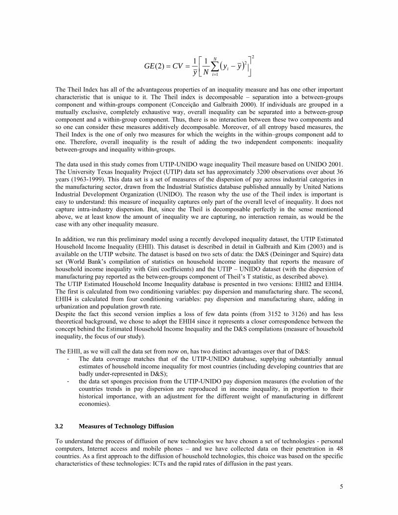
new technologies to exhibit slower diffusion rates where inequality is higher. This paper addresses this hypothesis. The next section describes the type of data collected thus far to perform preliminary explorations. 3. Measurement and Data Collection There are two obvious types of data required to test the hypothesis presented in section 2. The first are data of inequality, the second some measure of technological diffusion. The unit of analysis being considered in the study is the country, so we will need to look for measures of inequality and of technology diffusion for different countries. We consider first the data on inequality, which are based on two measures of wage dispersion captured through the Theil’s inequality measure and the estimated household income inequality (EHII). Inequality is then the key independent variable. Then, we look at measures of technology diffusion, as the dependent variables. Finally, we briefly describe other variables that may be important in determining the pace of technology diffusion, that is, other possible independent variables. 3.1 Measures of Inequality Interest on economic inequality has risen recently (see Atkinson, 1997, for example). But the measurement of inequality – that is, the measurement of the dispersion in the distribution of income – is a complex question (see Cowell, 1999). For example, Sen (1997) summarizes this complexity raising two issues regarding the meaning and use of inequality measures. First, inequality measures must encompass an objective element. Second, in some situations, they must allow for comparing alternative income distributions across a large number of people. As Conceição and Ferreira (2000) argue a measure of economic inequality provides, ideally, a number that summarizes the dispersion of the distribution of income among individuals. The measurement of inequality should encompass the differences in per capita income across populations within a country and across countries. There are many ways to measure inequality, all of which have some intuitive or mathematical appeal. However, we must be cautious because some measures of inequality have a perverse behavior. For instance, the variance is not independent of the income scale: doubling all incomes would produce a quadrupling of the estimate of income inequality (Litchfied 1999). For our purposes, it is important to consider a decomposable measure of inequality, for reasons that will become apparent later. The Generalized Entropy (GE) class of measures of inequality is the only one that is decomposable and satisfies the other criteria usually asked from inequality measures. The general formula for the measures in this class is

⎪⎭

⎪⎬⎫

⎪⎩

⎪⎨⎧

−⎟⎟⎠

⎞⎜⎜⎝

⎛−

= ∑=

111)(1

2

N

i

i

yy

NGE

α

ααα

where N is the number of people in the population, yi is the income of the ith person and y is the average income. α is a parameter that can take any real value. The two measures of inequality put forward by Theil are instances of this formula for α at 0 and 1:

∑=

⎟⎟⎠

⎞⎜⎜⎝

⎛==

N

i iyy

NLGE

1

ln1)0(

and

∑=

⎟⎟⎠

⎞⎜⎜⎝

⎛⋅==

N

i

ii

yy

yy

NTGE

1ln1)1( ,

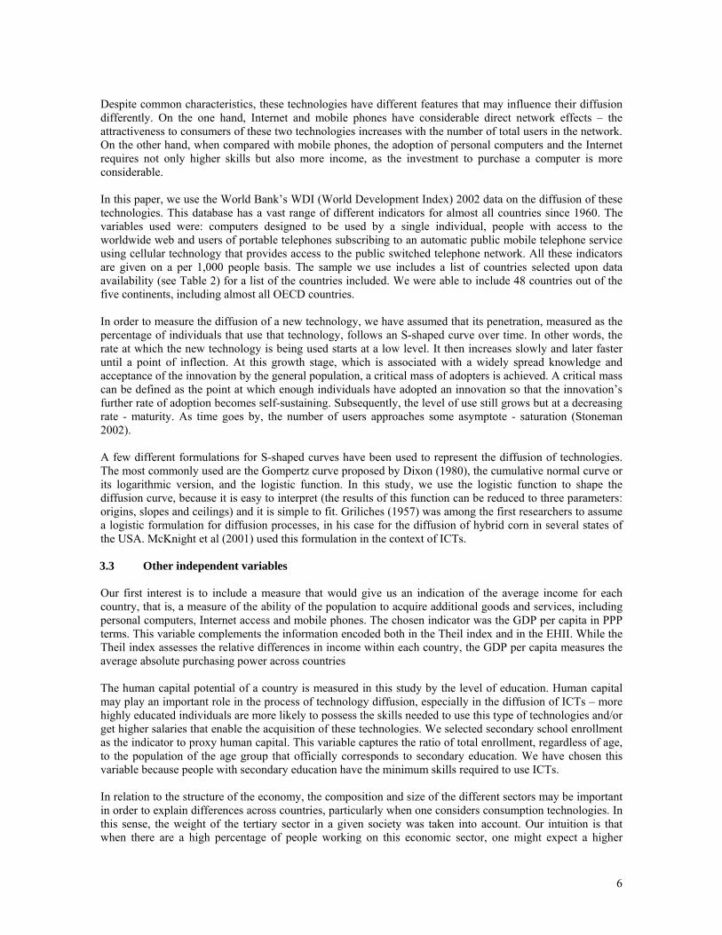
These measures are called, respectively, the mean log deviation and the Theil Index. Both of these measures are non-decreasing in inequality. Another well known member of this family of inequality measures is the coefficient of variation, obtained for α=2:

5

( )2

1

211)2( ⎥⎦

⎤⎢⎣

⎡−== ∑

=

N

ii yy

NyCVGE

The Theil Index has all of the advantageous properties of an inequality measure and has one other important characteristic that is unique to it. The Theil index is decomposable – separation into a between-groups component and within-groups component (Conceição and Galbraith 2000). If individuals are grouped in a mutually exclusive, completely exhaustive way, overall inequality can be separated into a between-group component and a within-group component. Thus, there is no interaction between these two components and so one can consider these measures additively decomposable. Moreover, of all entropy based measures, the Theil Index is the one of only two measures for which the weights in the within–groups component add to one. Therefore, overall inequality is the result of adding the two independent components: inequality between-groups and inequality within-groups. The data used in this study comes from UTIP-UNIDO wage inequality Theil measure based on UNIDO 2001. The University Texas Inequality Project (UTIP) data set has approximately 3200 observations over about 36 years (1963-1999). This data set is a set of measures of the dispersion of pay across industrial categories in the manufacturing sector, drawn from the Industrial Statistics database published annually by United Nations Industrial Development Organization (UNIDO). The reason why the use of the Theil index is important is easy to understand: this measure of inequality captures only part of the overall level of inequality. It does not capture intra-industry dispersion. But, since the Theil is decomposable perfectly in the sense mentioned above, we at least know the amount of inequality we are capturing, no interaction remain, as would be the case with any other inequality measure. In addition, we run this preliminary model using a recently developed inequality dataset, the UTIP Estimated Household Income Inequality (EHII). This dataset is described in detail in Galbraith and Kim (2003) and is available on the UTIP website. The dataset is based on two sets of data: the D&S (Deininger and Squire) data set (World Bank’s compilation of statistics on household income inequality that reports the measure of household income inequality with Gini coefficients) and the UTIP – UNIDO dataset (with the dispersion of manufacturing pay reported as the between-groups component of Theil’s T statistic, as described above). The UTIP Estimated Household Income Inequality database is presented in two versions: EHII2 and EHII4. The first is calculated from two conditioning variables: pay dispersion and manufacturing share. The second, EHII4 is calculated from four conditioning variables: pay dispersion and manufacturing share, adding in urbanization and population growth rate. Despite the fact this second version implies a loss of few data points (from 3152 to 3126) and has less theoretical background, we chose to adopt the EHII4 since it represents a closer correspondence between the concept behind the Estimated Household Income Inequality and the D&S compilations (measure of household inequality, the focus of our study). The EHII, as we will call the data set from now on, has two distinct advantages over that of D&S:

- The data coverage matches that of the UTIP-UNIDO database, supplying substantially annual estimates of household income inequality for most countries (including developing countries that are badly under-represented in D&S);

- the data set sponges precision from the UTIP-UNIDO pay dispersion measures (the evolution of the countries trends in pay dispersion are reproduced in income inequality, in proportion to their historical importance, with an adjustment for the different weight of manufacturing in different economies).

3.2 Measures of Technology Diffusion To understand the process of diffusion of new technologies we have chosen a set of technologies - personal computers, Internet access and mobile phones – and we have collected data on their penetration in 48 countries. As a first approach to the diffusion of household technologies, this choice was based on the specific characteristics of these technologies: ICTs and the rapid rates of diffusion in the past years.

6

Despite common characteristics, these technologies have different features that may influence their diffusion differently. On the one hand, Internet and mobile phones have considerable direct network effects – the attractiveness to consumers of these two technologies increases with the number of total users in the network. On the other hand, when compared with mobile phones, the adoption of personal computers and the Internet requires not only higher skills but also more income, as the investment to purchase a computer is more considerable. In this paper, we use the World Bank’s WDI (World Development Index) 2002 data on the diffusion of these technologies. This database has a vast range of different indicators for almost all countries since 1960. The variables used were: computers designed to be used by a single individual, people with access to the worldwide web and users of portable telephones subscribing to an automatic public mobile telephone service using cellular technology that provides access to the public switched telephone network. All these indicators are given on a per 1,000 people basis. The sample we use includes a list of countries selected upon data availability (see Table 2) for a list of the countries included. We were able to include 48 countries out of the five continents, including almost all OECD countries. In order to measure the diffusion of a new technology, we have assumed that its penetration, measured as the percentage of individuals that use that technology, follows an S-shaped curve over time. In other words, the rate at which the new technology is being used starts at a low level. It then increases slowly and later faster until a point of inflection. At this growth stage, which is associated with a widely spread knowledge and acceptance of the innovation by the general population, a critical mass of adopters is achieved. A critical mass can be defined as the point at which enough individuals have adopted an innovation so that the innovation’s further rate of adoption becomes self-sustaining. Subsequently, the level of use still grows but at a decreasing rate - maturity. As time goes by, the number of users approaches some asymptote - saturation (Stoneman 2002). A few different formulations for S-shaped curves have been used to represent the diffusion of technologies. The most commonly used are the Gompertz curve proposed by Dixon (1980), the cumulative normal curve or its logarithmic version, and the logistic function. In this study, we use the logistic function to shape the diffusion curve, because it is easy to interpret (the results of this function can be reduced to three parameters: origins, slopes and ceilings) and it is simple to fit. Griliches (1957) was among the first researchers to assume a logistic formulation for diffusion processes, in his case for the diffusion of hybrid corn in several states of the USA. McKnight et al (2001) used this formulation in the context of ICTs. 3.3 Other independent variables Our first interest is to include a measure that would give us an indication of the average income for each country, that is, a measure of the ability of the population to acquire additional goods and services, including personal computers, Internet access and mobile phones. The chosen indicator was the GDP per capita in PPP terms. This variable complements the information encoded both in the Theil index and in the EHII. While the Theil index assesses the relative differences in income within each country, the GDP per capita measures the average absolute purchasing power across countries The human capital potential of a country is measured in this study by the level of education. Human capital may play an important role in the process of technology diffusion, especially in the diffusion of ICTs – more highly educated individuals are more likely to possess the skills needed to use this type of technologies and/or get higher salaries that enable the acquisition of these technologies. We selected secondary school enrollment as the indicator to proxy human capital. This variable captures the ratio of total enrollment, regardless of age, to the population of the age group that officially corresponds to secondary education. We have chosen this variable because people with secondary education have the minimum skills required to use ICTs. In relation to the structure of the economy, the composition and size of the different sectors may be important in order to explain differences across countries, particularly when one considers consumption technologies. In this sense, the weight of the tertiary sector in a given society was taken into account. Our intuition is that when there are a high percentage of people working on this economic sector, one might expect a higher

7

consumption of household ICTs. If a considerable fraction of the population makes use of ICTs at work, it is then probable that the diffusion of these technologies as a final consumer good may growth relatively faster. The indicator used to measure the weight of the tertiary sector in the economy is the percentage of value added that is due to service sectors (that is, ISIC 50-99). The data source used for these variables is the WDI 2002. In the future, we are planning to include more independent variables to improve the explanatory power of our model. If necessary, the current data will be reviewed. Other authors that studied the diffusion of ICTs were sensible to the relevance of other independent and controlling variables for understanding the process of technology diffusion and included some economic and social variables in their studies. For instance, Gebread (2002) conducted a study about the diffusion of mobile telecommunications in 41 African countries between 1987 and 2000 employing a fixed effects model. The results indicate that competition is the main driving force behind telecommunications widespread use, duopolies and triopolies grow faster than monopolies. This study also found that privatization, digitalization and urbanization are significant determinants in the diffusion of mobile phones. In a study about the diffusion of the Internet in some OECD countries, Hargittai (1999) included several variables such as level of English expertise, the existence of monopoly (as related to telecommunications policy), the prices of accessing the Internet, and phone density (as a proxy for infrastructure). In this study, the author found that economic factors alone did not explain Internet connectivity, and that telecommunications policy and infrastructure were important variables. In a more recent study still about the diffusion of Internet, Beilock and Dimitrova (2003) found that not only income appeared to be important, but also the openness of the society (understood as high or low level of civil liberties) and infrastructure (including number of personal computer and number of telephone per thousand people) play a role in explaining the level of technology diffusion. Hall and Khan (2002), in a review article on adoption of technologies, based on previous empirical and non-empirical studies, suggested that market structure (presence or absence of competition), the regulatory environment and governmental institutions have powerful effects on technology adoption. Later versions of the work presented in this paper should consider some of these independent variables, which in some contexts in the past have seemed to explain differences in the proliferation of new technologies across countries. 3.4 Limitations The data collected and used in this paper has several limitations that are worth mentioning. The main limitation of the UTIP dataset is that industrial pay inequality is only a component of overall income inequality, but the relative importance of industrial wages inequality differs across countries and over time depending on the structure of the economy. In addition to the industry, the agriculture (primary sector) and the services (tertiary sector) sectors may play an important role in the overall economy, depending on the country. Even though Conceição and Galbraith (2001) have shown that the dynamics of the industry Theil do follow those of the overall economy’s, we are using in this paper levels of inequality, rather than rates of change. Still, the EHII data set, as Galbraith and Kim (2003) suggest, goes around this difficulty. With respect to the data used to characterize the diffusion of technology, also there exist gaps in the time series that may reduce our confidence in the results obtained: (a) the technologies we are studying were introduced in the market very recently, thus it is impossible to have a comprehensive long time series to use in our regression analyses; (b) the three technologies analyzed belong to the ICTs sectors and therefore the results may be biased by the common characteristics of these technologies and, as a result, the findings cannot yet be applied to other contexts; (c) the data available about the penetration rate of the three technologies studied did not consider the purpose for what the technology was purchased, thus there is no differentiation between the adoption of the technology for household use and corporate use. The independent variables used in our analysis may explain differently the adoption of technology by household and by corporations, but we are not able to capture such effect, which might be small if adoption trends do not vary much between the two segments of the economy.

8

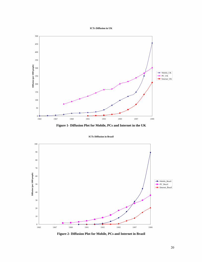
The choice and analysis of the independent variables provided here is at a preliminary stage, so will be our conclusions. We are aware of these limitations and hope to include in the future other variables in the model, especially variables that account for non-economic aspects, such as social and political elements that enhance and sometimes hinder the diffusion of new technologies. 4. Model and Methodology This section presents the models devised to explain the diffusion of ICTs and its possible relationships to inequality and to the other macro socio-economic variables considered in this study. This section also discusses the methodologies applied to estimate such models. The first sub section looks at the model used to explain the proliferation of ICTs within each country. The second sub section discusses the model used to explain the different rates of diffusion of ICTs found across countries. 4.1 The diffusion of ICTs within countries The diffusion of a new technology in a country follows usually an S-shaped curve. This is the case for the penetration of personal computers, Internet access and mobile phones, as mentioned before (see figures 1 through 4). The cumulative normal and the logistic curves are among the most used formulations for the diffusion of technology in the literature. Following Griliches (1957), the logistic growth curve is defined by P=K/(1+e-(a+bt)), where P is the percentage of penetration of the new technology, K the ceiling value, t the time variable, b the rate of growth coefficient and a the constant that allows for shifting the S-curve in the time domain. By dividing both sides by K-P and taking the logarithm, we get a linear relationship, log[P/(P-K)]=a+b.t, which allows for estimating the parameters of the S-curve directly by least squares. The value of K is assumed to be 100%, since each of the three technologies considered can, theoretically, be used by each and every person individually. However, we know that even in the long run, the penetration of a new technology hardly rises up to such level. Looking at data from the WDI about the penetration of mature technologies, like Television sets and Telephone Mainlines, in the US (country where these technologies diffusion has stabilized) we notice that the ceiling of diffusion is between 70% and 90%. Later versions of this work should consider estimating the ceiling value more carefully. Additionally, we can observe that a and b are related by the expression a=log[(α/(1-α)]-b.tα, where α is a level of proliferation of the technology (in percentage terms, therefore between 0 and 1) and tα is the time for which such level is obtained. Hence, we are interested in estimating the model log[(1-α)P/(α(P-K))]=b.t+εt, where εt is the error term. This model can be easily estimated with linear least squares without a constant term. We have fitted an S-shaped curved to the proliferation of each of the three technologies considered for each of the countries used in our analysis. Each S-shaped curve is estimated separately. Note that this procedure generates a rate of growth coefficient for each country for each technology. In other words, the logistic curves serve as a summary device collapsing the levels of penetration of the new technology over time into the rate of growth coefficient. Then, we set up a vector with all these coefficients, b(c,τ), where c indicates the country and τ the technology. 4.2 Linking diffusion rates to macro socio-economic variables The goal of the second part of our work is to assess the relationship between the rate of growth coefficient, b(c,τ), and socio-economic variables across countries. In estimating this relationship, we expect to explain how the proliferation of a new technology depends on these variables, following the ideas discussed in the previous sections.

9

Consider a single technology and the vector of rate of growth coefficients for that technology bτ(c)=b(c,τ). We set up the model

bτ(c)=X(c).βτ+µτc where X(c) is a vector of independent variables used to explain variance in bτ(c) and µτc is the error term. As our major goal is to relate the diffusion of technology to inequality, X(c) will include the level of inequality for the countries considered. X(c) will also include other variables, such as the GDP per capita, a proxy for the level of education and an indicator of the influence of the tertiary sector in the economic structure of the country, as discussed in section 3.4. A limitation of this model is that we write the rate of growth coefficient for each technology separately. However, we know that the proliferation of one technology influences markedly the diffusion of other technologies (see Table 1 where we report the coefficients of correlation between the three technologies studied). This is an issue that should be addressed carefully in later versions of this work, for example considering a system of simultaneous equations. Just as we summarized the proliferation of each technology per country and therefore collapsed this time series into a single number, the rate of growth coefficient for that technology and that country, we need to follow the same approach with regards to the variables in X(c), so that we can estimate the model above across countries. In lack of a consistent theory to do so, we took, for each independent variable, its average over the appropriate time period. For example, for the level of inequality, we averaged out, for each country, the Theil Index over the time period between 1985 and 1999, that is, we have constructed the vector:

),(1)(1

icTheilIndexN

cIN

i∑=

=

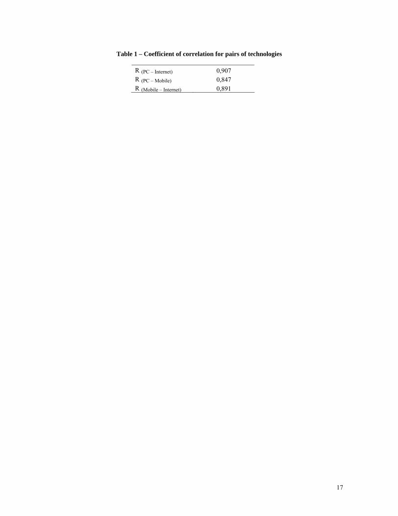
We proceeded likewise for all the other independent variables and obtained X(c). The vector of coefficients in our model βτ indicates the relationship between the rate of growth coefficient and the independent variables across countries for each technology. Recall that a higher b coefficient indicates a faster technology proliferation. Therefore, a priori, we expect inequality to be negatively correlated with the dependent variable (b or the rate of growth coefficient). On the contrary, we expect both the GDP per capita ppp and the level of education to be positively correlated with the dependent variable. 5. Preliminary Results This section summarizes a range of the preliminary empirical results obtained so far. First, we look at the diffusion rates of the ICTs considered in the paper. Then we present the results of estimating the parameters of the S curves, followed by the preliminary results of the empirical estimates of the determinants of technological diffusion. 5.1 Relationship among the diffusion of different ICTs We start by noting that there is a strong interaction among the evolution of the penetration of the three technologies studied. Also along time, it is possible that one technology exert some influence on the diffusion of another technology that somehow has a connection to the former. We began by performing a bivariate analysis on the penetration of each technology over time that allows for calculating the coefficients of correlation for each pair of technologies. Table 1 depicts the results. It is worth noting that there is a positive and strong association between the three technologies that we are studying, especially in the case of ownership of personal computers and Internet access. While this might not be surprising because today it is still very likely that one needs a computer to connect to the Internet, the strong association between PCs and mobiles and between mobiles and the Internet shows that technologies in

10

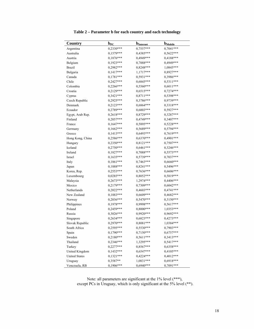
the information revolution are very much tied to each other and the use of one of them clearly prompts the use of the others, especially when the diffusion of newer ICTs that enable to use the internet through cell phones The above observation indicates that when examining the diffusion of one technology, one must relate it to the diffusion of the other technologies, for example, because of the, sometimes sine qua non, need of having one technology to use the other. However, we also observe that after a certain critical mass of users has been achieved, the growth of the penetration rate of a technology is self-sustained given the network effects, therefore less dependent on the penetration of complementary technologies. That is, two regimes in the relationship between the diffusion of ICTs and the complementarity among these technologies might be expected. 5.2 Results of the fitting of S-shaped curves This section presents and discusses the results of fitting S-shaped curves to the proliferation of ICTs, for each technology and for each country, obtained by computing the parameter b of the logistic function by employing least squares on the logarithmic transformation suggested in section 3. Table 2 shows the coefficients b(c,τ) obtained. We have 144 coefficients, since we have 48 countries and 3 technologies to consider for each country. All the regressors are statistically significant for the three technologies at the 1% level, with the exception of Uruguay for the diffusion of personal computers, which is significant at the 5% level. Additionally, the R2 for the regressions ran vary between 0.6487 and 0.9971, which are high. Hence, the results confirm the hypothesis that the S-shaped curves are good functional forms to explain the diffusion of ICTs within countries. If we remember that there is a positive relationship between the rate of growth coefficient b and the proliferation of technology, we can conclude that the technology with a slower diffusion rate is Personal Computers, since bPC is always the lowest coefficient for each country. It seems convenient to understand why the rate of coefficient growth for personal computers is the smallest of the three rates computed. One potential reason is that the initial investment required to buy a personal computer is substantially superior in comparison to the investment needed for example to use a mobile phone. The technology associated with a PC is older than the others analyzed in this paper, which implies that the diffusion’s stage of PC could be more advanced than for other ICTs. Thus, the growth of mobile and Internet access is higher also because there is a gap to fill until they reach the same diffusion’s stage of PCs (this also can be observed in the diffusion plots in the figures 1 through 4). Another possible explanation relates to skills. The PC technology is much more skill intensive that the other technologies considered, mobile phones and the Internet. In reality, the skill-demanding characteristic of PC conditions the rate of coefficient growth of the diffusion of such technology. Finally, it is also possible to observe that at least two thirds of the countries in this sample present a value for parameter b referring to Internet access greater than the respective value for mobile. The remaining countries, with a few exceptions, seem to belong to a group of less developed nations. This would suggest that these countries “leapfrog” to using mobile phones without having used the Internet so much. However, such an analysis must deserve caution. It might be that these countries cannot use so much the Internet because there is no installed PC based that allows for doing so. To delve more seriously into this issue one should characterize the investments in ICTs in these countries in order to understand to what extent it is easier to deploy wireless technologies and mobile phones rather than computer networks. Other possible explanations for the use of mobile phones as a substitute to fixed phones in less developed societies include the fact that the poor cannot afford installation costs and that fixed lines are not easily available in the market due to infrastructure limitations. 5.3 Results of explaining the parameters of the S-curves The previous section estimated the growth coefficient for the logistic curves aimed at capturing the diffusion of ICTs in each country considered. This section relates these coefficients to the macro socio-economic

11

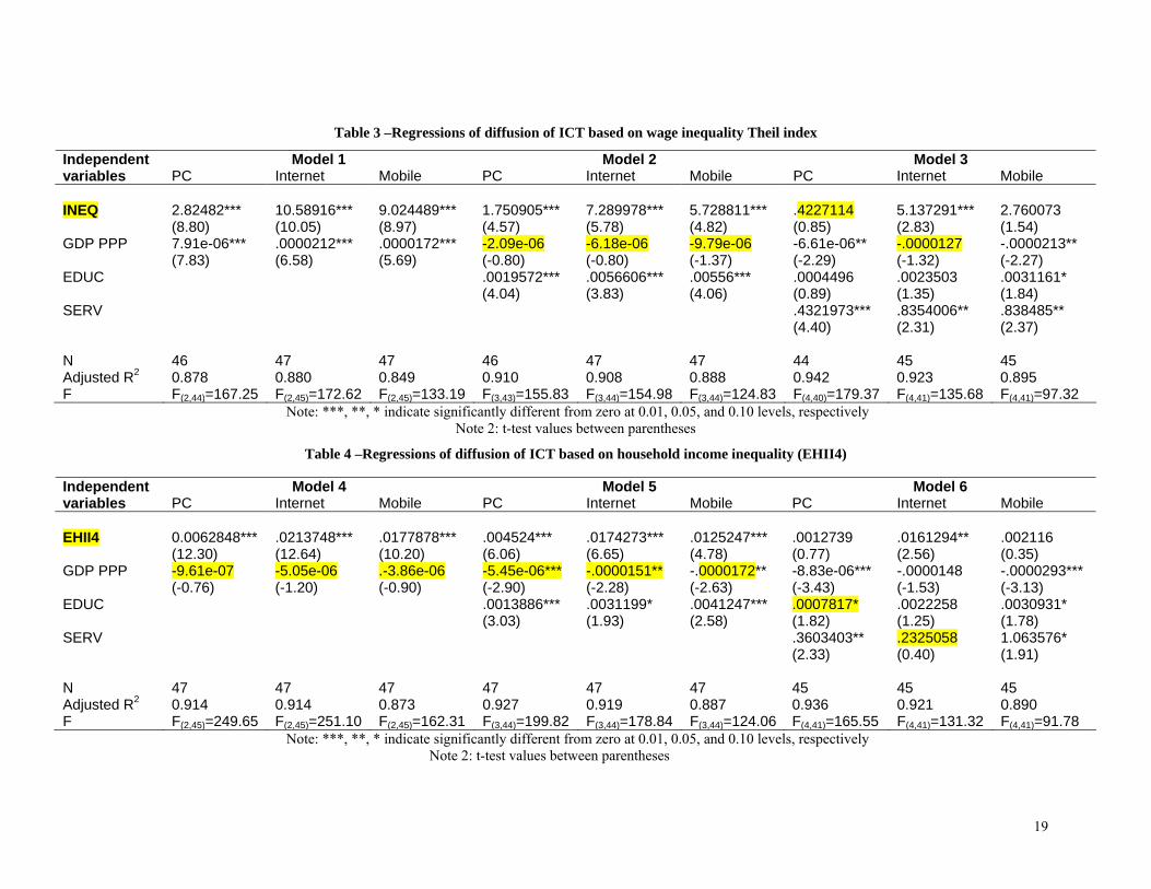
variables discussed in section 3.3 and in section 4.2, as a way to explain the relationship between these variables and the diffusion of ICTs. Therefore, we have considered a set of models in which we write the growth coefficient as a function of these variables. The first model includes two independent variables: economic inequality, measured by the Theil Index and represented by INEQ in our model, and a variable that gauges the ability of the population to acquire additional goods and services - the gross domestic product per capita converted to international dollars using purchasing power parity rates (GDP PPP):

bτ(c) = α1.INEQ(c) + α2.GDP PPP(c) + ε(c) Equation 1 – Model 1

The first column in Table 3 shows the results obtained from estimating this model with linear least squares. We observe that inequality has a positive correlation to the rate of growth coefficient and is always significant at the 1% level. Therefore, our study indicates that the diffusion of technology increases with higher levels of inequality. This fact could be explained by the hypothesis of Galbraith (1998) that suggests that that new commodities diffuse from the rich to the masses. In an unequal society, with an economic elite, it would be easier to introduce new technologies, and so one would expect that these new consumer goods become part of the everyday life even for low-income households. As new technologies become mature, their prices fall, and they become available to poorer people at substantially lower prices than were first paid by the economic elites. As expected, the GDP PPP is positively correlated with the dependent variable and statistically significant at the 1% level for all the three technologies considered. Additionally, note that for this model and for all the three technologies considered, the adjusted R2 are high (between 0.85 and 0.88) and the F-statistics for the whole models are high as well (greater than 100.00), which attests for the explanatory power of this model. The second model considers the introduction of an additional independent variable to complement the explanatory power of Theil Index and GDP PPP. This variable, named EDUC in the model, is used to proxy the level of human capital. The relevance of this variable is easily explained by the argument that more highly educated individuals are likely to possess the appropriate skills needed to use ICTs more efficiently. The second model estimated is

bτ(c) = α1.INEQ(c) + α2.GDP PPP (c) + α3.EDUC (c) + ε (c) Equation 2 – Model 2

The second column in Table 3 shows the results obtained from estimating this model using least squares. The most relevant and surprisingly result is that the sign of the coefficient associated with GDP PPP changes from positive to negative, but the coefficients are not statistically significant at all. In addition, the variable EDUC is positively related to the dependent variable and statistically significant at the 1% level.. By comparing the adjusted R2 of the two models discussed so far, it seems relevant to point out that the second model is a better fit than the previous one as the adjusted R2 range from 0.89 and 0.91.. Despite the fact that we cannot fully understand the sign change of the coefficient in GDP PPP, the introduction of the EDUC variable contributes positively to explain the variance in the growth coefficients associated with the diffusion of ICTs. The third model devised includes the same variables as model 1 and model 2, plus a variable related to the economic structure of the country - the value added of the services sector as % of the GDP, which we have called SERV. The model to estimate is

bτ(c) = α1.INEQ (c) + α2.GDP PPP (c) + α3.EDUC (c) + α4.SERV (c) + ε (c) Equation 3 – Model 3

12

The results obtained from estimating this model are shown in the last column of table 3. The new independent variable, which reflects the contribution of the tertiary sector in the economic structure of the countries, is also statistically significant at the 5% level. The overall fitness of the model increases from the previous models as its adjusted R2 ranges from 0.89 to 0.94. However, the variable EDUC is only significant for the case of the mobile phones at the 10%. This suggests that we might have to rethink the proxy we are using for the level of human capital. Or, alternatively, that there is a significant correlation among the independent variables that might have to be addressed with more sophisticated econometric methods. In model 3, the variable INEQ becomes less significant. In fact, it is statistically significant only for the case of the internet which is significant at the 1% level. It is therefore interesting to understand why the explanatory power of inequality seems to decrease from model 1 to model 3. We believe that further analysis and in depth study of other independent variables (including the relationships among them) may contribute to shed light on these issues and sharpen our knowledge and understanding of the relationship between inequality and the diffusion of ICTs. The following models are the outcome of a substitution of the variable that measures economic inequality. Instead of using the wage inequality Theil index from UTIP, the models 4-6 include a variable that measure the household income inequality (EHII). As referred above, the main difference between the Theil index from UTIP and EHII4 is that the former pertains only to economic inequality across the industrial sector and the latter is wider in the sense that includes annual estimates of household income inequality for most countries. Looking at Table 4 it is possible to observe that the model 4 presents better measures of goodness of fit (adjusted R2 and F-statistic) when compared with model 1.

bτ(c) = α1.EHII4(c) + α2.GDP PPP(c) + ε(c) Equation 4 – Model 4

The fourth model shows that the variable GDP PPP is not statistically significant for none of the three technologies. It is worth remembering that in model 1 this variable is significant at the 1% level. Computing the coefficient of correlation between the two measures of inequality used in the models and the GDP PPP it is possible to see that the results show a low level of association between the variables. The fifth model is composed by the same variables of the second model with the substitution of the Theil index by the EHII4.

bτ(c) = α1.EHII4(c) + α2.GDP PPP (c) + α3.EDUC (c) + ε (c) Equation 5 – Model 5

Model 5, when compared with model 2 also presents better adjusted R2 and F-statistic (see Table 4). In Model 5 all variables are statistically significant. The main change is that GDP ppp becomes significant while it was not in Model 2. The last model presented is similar to model 3 with the exception of the variable concerning economic inequality.

bτ(c) = α1.EHII4 (c) + α2.GDP PPP (c) + α3.EDUC (c) + α4.SERV (c) + ε (c) Equation 6 – Model 6

There are some relevant differences between the models 3 and 6, namely in the case of PC technology. The inequality measure is only significant for the Internet. In the case of EDUC, the main change from Model 3 is that it becomes significant for PCs. With respect to the Internet, the variable SERV is not longer significant Finally, about the mobile technology there are not relevant differences between these two models. In sum, we could say that using the EHII4 yield results that are similar to those obtained with the Theil index, although if comparing all the six models, Model 3 shows a better fit. There are differences in the precision

13

with which estimates are measured in the different models, but the substantive results are very similar in both cases. 6. Conclusions This study is a preliminary work of a long term project about the relationships between inequality and technology diffusion. Thus, it is our purpose to upgrade and improve in several aspects what we have done so far. First, the logistic curve’s K parameter will have to be adjusted. In this analysis was assumed that the upper limit to technology penetration is 100%, which is an assumption that needs to be justified with existing empirical studies and may be modified. In relation to the technology diffusion measurement, it is planed to test other methods to estimate the evolution of S-shaped curve of diffusion (Gompertz, cumulative normal, cumulative log-normal and other epidemic models). Simultaneously, as referred in section 4, is important to construct an equation system that includes the diffusion of all technologies in order to capture interaction across technologies. It is also important to study other technologies such as passenger cars, other household technologies, to avoid a possible bias by focusing only in the diffusion of new and information technologies. With respect to the inequality measurements we wish to develop new Theil index series that measure inequality across all sectors of society – as referred in section 2.1, as the Theil coefficient used here pertains only to economic inequality across the industrial sector. In addition, and with respect to the EHII, we want to study the implications of this dataset, namely the interaction with the conditioning variables in the measurement of inequality. Finally, is necessary to review the independent variables included in the model in order to increase the fitting of the model to what indeed goes on in the real world (and for that, we might have to consider variables to measure the extent of the telecommunications infrastructure, the level of civil rights, monopoly power, hedonic technology prices). This preliminary work has shown that, as we expected, the level of inequality in a given society plays an important role in the diffusion of ICTs, although we expected to find the opposite effect. Our assumption was that the diffusion of technology would be hindered by economic inequality, but the empirical model suggests the opposite is the case. This does not mean the total rejection of our hypothesis, at least not until we continue working in the model in different directions. One is obviously to find better proxies for some of the variables used to represent human capital. Another is to include and test other possible independent and controlling variables, such as telecommunications policy framework, whether countries have competition and or public/private telecommunications providers, prices of the technologies and services related to ICTs. Moreover, one important step would be to advance in the elaboration of a new data set that encompasses more comprehensive information about inequality. We believe it is important to account for other sectors of the economy, or at least, at the minimum we should be able to find out if inequality in the industrial sector behave similarly as inequality in other sectors of the economy, especially for countries where services and agriculture are the base of economic activities and where ICTs also are supposed to proliferate. As a preliminary report of the on-going research project, we could state the following:

• Preliminary results seem to reject the original hypothesis formulated; • This rejection cannot, at this stage, be considered firm because there is still work to do in terms of:

o Better defining the type of data used to translate into quantitative terms the concepts being advanced (namely in terms of the inequality measure; if it is likely that the most important source of income used to buy the consumption technologies are wages, we are not considering at present the entire service sector);

o Ameliorating the estimating of the model, to correct, or account for, obvious collinearity between independent variable and the very likely endogeneity between inequality and technological diffusion;

o Better capturing the consumption side of the economy, which is not completely captured with the data at present;

14

• Still, it is at least possible that using better data and econometric techniques will not change substantially the essence of the results, and a conceptual effort needs to be undertaken to attempt to explain what may turn out to be a surprising result, in light of our original hypothesis.

15

References Acemoglu, D. (2002a). “Technical Change, Inequality and the Labor Market,” Journal of Economic

Literature, 40: 7-72. Acemoglu, D. (2002b). “Cross-country Inequality Trends,” Economic Journal, 113 (485): F121-F149 Sp. Iss.

F. Acemoglu, D., and Pieshcke, J. S. (2000). “Certification of Training and Training Outcomes,” European

Economic Review, 44: 917-927. Acemoglu, D., and Zilibotti, F. (2001). “Information Accumulation in Development,” Journal of Economic

Growth, 4: 5-38. Aghion, P., Caroli, E., and Peñalosa, C. G. (1999). “Inequality and Economic Growth: The Perspective of the

New Growth Theories,” Journal of Economic Literature, 37: 1615-1660. Aghion, P., and Williamson, J. G. (1998). Growth, Inequality and Globalization. Cambridge; Cambridge

University Press. Atkinson, A. B. (1997). "Bringing Income Distribution in from the Cold," The Economic Journal, 107: 291-

321. Autor, D. H., Katz, L. F., and Krueger A. B. (1998). “Computing Inequality: Have Computers Changed the

Labor Market,” Quarterly Journal of Economics, 113: 1169-1213. Beilock, R., and Dimitrova, D. V. (2003). “An Exploratory Model of Inter-country Internet Diffusion,”

Telecommunications Policy, 27: 237-252. Bound, J, and Johnson, G. (1992). “Changes in the Structure of Wages in the 1980s – An Evaluation of

Alternative Explanations,” American Economic Review, 82: 371-392. Borghans, L. A., and ter Weel, B. (2002). “The Diffusion of Computers and the Distribution of Wages,” ROA

working paper series number 3. Card, D. and Lemieux, T. (2000). “Can Falling Supply Explain the Rising Return to College for Younger

Men? A Cohort-based Analysis,” Quarterly Journal of Economics, 116: 705-746. Caselli, F. (1999). “Technological Revolutions,” American Economic Review, 89: 78-102 Castells, M. (1996). The Rise of the Network Society, The Information Age: Economy, Society and Culture,

Vol. I. Oxford; Blackwell Publishers Ltd. Castells, M. (1998). “Information Technology, Globalization and Social Development” Paper prepared for the

UNRISD Conference on Information Technologies and Social Development. Conceição, P., and Ferreira, P. (2000). “The Young Person’s Guide to the Theil Index: Suggesting Intuitive

Interpretations and Exploring Analytical Applications,” UTIP working paper number 14. Conceição, P., and Galbraith, J. K. (2000). “Constructing Long and Dense Time-Series of Inequality Using

the Theil Index,” Eastern Economic Journal, 26: 61-74. Cowell, F. A. (1999) “Measurement of Inequality,” in Atkinson, A. B. and Bourguignon F. (eds) Handbook of

Income Distribution, North Holland, Amsterdam. DiNardo, J., and Pischke, J. S. (1997). “The Returns to Computer Use Revisited:

Have Pencils Changed the Wage Structure too?,” The Quarterly Journal of Economics, 112: 291-303.

Dixon, R. (1980). “Hybrid Corn Revisited,” Econometrica, 48: 1451-1461 Easterly, W. (2002). “Inequality does Causes Underdevelopment: New evidence

from commodity endowments, middle class share, and other determinants of per capita income,” Center for Global Development working paper number 1.

Galbraith, J. K., and Kum, H. (2003). “Estimating the Inequality of Household Incomes: Filling Gaps and Correcting Errors in Deininger & Squire,” UTIP working paper number 22.

Galbraith, J. K. (1998). Create Unequal: The Crisis in American Pay. New York, The Free Press. Gebreab, F. A. (2002). “Getting Connected: Competition and Diffusion in African Mobile Communications

Markets,” World Bank Policy Research working paper number 2863 Griliches, Z. (1957). “Hybrid Corn: An Exploration in the Economics of Technological Change,”

Econometrica, 25: 501-522. Hall, B. H., and Khan, B. (2003, forthcoming). “Adoption of New Technology,” Draft of an article for

publication in Jones, Derek C., Handbook of Economics in the Electronic Age, Academic Press. Hargittai, E. (1999). “Weaving the Western Web: Explaining Differences in Internet Connectivity among

OECD Countries,” Telecommunications Policy, 23: 701-718.

16

Krueger, A. B. (1993). “How Computers have Changed the Wages Structure – evidence from microdata, 1984-1989.” Quarterly Journal of Economics, 108: 33-60.

Krussel, P., Ohanian, L. E., Ríos-Rull, J. V., and Violante, G. L. (1997). “Capital-Skill Complementarity and Inequality: a macroeconomic analysis,” Federal Reserve Bank of Minneapollis staff report number 236.

Kuznets, S. (1963). "Quantitative Aspects of the Economic-Growth of Nations," Economic Development and Cultural Change, 11: 1-80.

Litchfield, J. A. (1999). “Inequality Methods and Tools,” Text for World Bank’s Web Site on Inequality, Poverty, and Socio-economic Performance.

McKnight, L. W. and M. S. Shuster (2001), “After the Web: Diffusion of Internet Media” in McKnight, L. W. Lehr, W. and Clark, D. D. (eds.) Internet Telephony, Cambridge, Massachusetts, The MIT Press: 165-190

Norris, P. (2001). Digital Divide? Civic Engagement, Information Poverty & the Internet Worldwide. New York; Cambridge University Press.

Sachs, J. (2002). “The Global Innovation Divide,” National Bureau Economic Research, www.nber.org/books/innovation3/sachs5-22-02.pdf.

Schmitt, J. (1995). “The Changing Structure of Male Earnings in Britain, 1974-88,” in Differences and changes in wage structures, (ed.) Freeman R and Katz L, University of Chicago Press.

Sen, A. K. (1997; 1st ed. 1973). On Economic Inequality. Oxford; Clarendon Press Oxford University Press. Stoneman, P. (2002). The Economics of Technological Diffusion. Oxford; Blackwell Publishers Ltd. UTIP (2002). “UTIP UNIDO Theil 2001”, Austin Texas: UTIP. Vindigni, A. (2002). “Income distribution and Skilled Biased Technological Change,” Princeton, Department

of Economics - Industrial Relations Sections working paper number 464, www.irs.princeton.edu/pubs/pdfs/464.pdf.

World Bank (2002). “World Development Indicators”, Washington DC: The World Bank.

17

Table 1 – Coefficient of correlation for pairs of technologies

R (PC – Internet) 0,907 R (PC – Mobile) 0,847 R (Mobile – Internet) 0,891

18

Table 2 – Parameter b for each country and each technology

Note: all parameters are significant at the 1% level (***),

except PCs in Uruguay, which is only significant at the 5% level (**).

Country bPC bInternet bMobile Argentina 0,2330*** 0,7557*** 0,7041*** Australia 0,1579*** 0,4385*** 0,5622*** Austria 0,1876*** 0,4949*** 0,4188*** Belgium 0,1923*** 0,7888*** 0,4949*** Brazil 0,2982*** 0,8248*** 1,0845*** Bulgaria 0,1417*** 1,1717*** 0,8927*** Canada 0,1781*** 0,5931*** 0,3986*** Chile 0,2427*** 0,6845*** 0,5311*** Colombia 0,2266*** 0,5560*** 0,6011*** Croatia 0,2129*** 0,6515*** 0,7274*** Cyprus 0,3421*** 0,8711*** 0,5398*** Czech Republic 0,2925*** 0,3786*** 0,9739*** Denmark 0,2123*** 0,6864*** 0,3318*** Ecuador 0,2789*** 0,6003*** 0,5927*** Egypt, Arab Rep. 0,2618*** 0,8729*** 0,3287*** Finland 0,2057*** 0,4749*** 0,3407*** France 0,1647*** 0,5895*** 0,5228*** Germany 0,1662*** 0,5689*** 0,5794*** Greece 0,1413*** 0,6493*** 0,7619*** Hong Kong, China 0,2586*** 0,6370*** 0,4901*** Hungary 0,2350*** 0,8121*** 0,7507*** Iceland 0,2750*** 0,6461*** 0,3246*** Ireland 0,1827*** 0,7088*** 0,5573*** Israel 0,1635*** 0,5739*** 0,7037*** Italy 0,1861*** 0,7463*** 0,6660*** Japan 0,1888*** 0,8241*** 0,5496*** Korea, Rep. 0,2553*** 0,7636*** 0,6606*** Luxembourg 0,0285*** 0,8052*** 0,5819*** Malaysia 0,2673*** 1,2974*** 0,4406*** Mexico 0,2179*** 0,7309*** 0,6042*** Netherlands 0,2022*** 0,4603*** 0,4741*** New Zealand 0,1883*** 0,6609*** 0,4682*** Norway 0,2036*** 0,5470*** 0,3150*** Philippines 0,1978*** 0,9998*** 0,5617*** Poland 0,2459*** 0,8000*** 1,0353*** Russia 0,3026*** 0,9920*** 0,9692*** Singapore 0,2634*** 0,6823*** 0,4273*** Slovak Republic 0,2970*** 0,8081*** 1,0384*** South Africa 0,2595*** 0,5530*** 0,7903*** Spain 0,1790*** 0,7150*** 0,6757*** Sweden 0,2180*** 0,5611*** 0,3413*** Thailand 0,2346*** 1,3295*** 0,5417*** Turkey 0,2277*** 0,8567*** 0,6358*** United Kingdom 0,1432*** 0,6547*** 0,4105*** United States 0,1321*** 0,4224*** 0,4012*** Uruguay 0,3587** 1,0831*** 0,6918*** Venezuela, RB 0,1906*** 0,6940*** 0,7091***

19

Table 3 –Regressions of diffusion of ICT based on wage inequality Theil index

Note: ***, **, * indicate significantly different from zero at 0.01, 0.05, and 0.10 levels, respectively Note 2: t-test values between parentheses

Table 4 –Regressions of diffusion of ICT based on household income inequality (EHII4)

Note: ***, **, * indicate significantly different from zero at 0.01, 0.05, and 0.10 levels, respectively Note 2: t-test values between parentheses

Model 1 Model 2 Model 3 Independent variables PC Internet Mobile PC Internet Mobile PC Internet Mobile INEQ 2.82482***

(8.80) 10.58916*** (10.05)

9.024489*** (8.97)

1.750905*** (4.57)

7.289978*** (5.78)

5.728811*** (4.82)

.4227114 (0.85)

5.137291*** (2.83)

2.760073 (1.54)

GDP PPP 7.91e-06*** (7.83)

.0000212*** (6.58)

.0000172*** (5.69)

-2.09e-06 (-0.80)

-6.18e-06 (-0.80)

-9.79e-06 (-1.37)

-6.61e-06** (-2.29)

-.0000127 (-1.32)

-.0000213** (-2.27)

EDUC .0019572*** (4.04)

.0056606*** (3.83)

.00556*** (4.06)

.0004496 (0.89)

.0023503 (1.35)

.0031161* (1.84)

SERV .4321973*** (4.40)

.8354006** (2.31)

.838485** (2.37)

N 46 47 47 46 47 47 44 45 45 Adjusted R2 0.878 0.880 0.849 0.910 0.908 0.888 0.942 0.923 0.895 F F(2,44)=167.25 F(2,45)=172.62 F(2,45)=133.19 F(3,43)=155.83 F(3,44)=154.98 F(3,44)=124.83 F(4,40)=179.37 F(4,41)=135.68 F(4,41)=97.32

Model 4 Model 5 Model 6 Independent variables PC Internet Mobile PC Internet Mobile PC Internet Mobile EHII4 0.0062848***

(12.30) .0213748*** (12.64)

.0177878*** (10.20)

.004524*** (6.06)

.0174273*** (6.65)

.0125247*** (4.78)

.0012739 (0.77)

.0161294** (2.56)

.002116 (0.35)

GDP PPP -9.61e-07 (-0.76)

-5.05e-06 (-1.20)

.-3.86e-06 (-0.90)

-5.45e-06*** (-2.90)

-.0000151** (-2.28)

-.0000172** (-2.63)

-8.83e-06*** (-3.43)

-.0000148 (-1.53)

-.0000293*** (-3.13)

EDUC .0013886*** (3.03)

.0031199* (1.93)

.0041247*** (2.58)

.0007817* (1.82)

.0022258 (1.25)

.0030931* (1.78)

SERV .3603403** (2.33)

.2325058 (0.40)

1.063576* (1.91)

N 47 47 47 47 47 47 45 45 45 Adjusted R2 0.914 0.914 0.873 0.927 0.919 0.887 0.936 0.921 0.890 F F(2,45)=249.65 F(2,45)=251.10 F(2,45)=162.31 F(3,44)=199.82 F(3,44)=178.84 F(3,44)=124.06 F(4,41)=165.55 F(4,41)=131.32 F(4,41)=91.78

20

ICTs Diffusion in UK

0

50

100

150

200

250

300

350

400

450

500

1985 1987 1989 1991 1993 1995 1997 1999

Diff

usio

n (p

er 1

000

peop

le)

Mobile_UKPC_UKInternet_UK

Figure 1- Diffusion Plot for Mobile, PCs and Internet in the UK

ICTs Diffusion in Brazil

0

10

20

30

40

50

60

70

80

90

100

1985 1987 1989 1991 1993 1995 1997 1999

Diff

usio

n (p

er 1

000

peop

le)

Mobile_BrazilPC_BrazilInternet_Brazil

Figure 2- Diffusion Plot for Mobile, PCs and Internet in Brazil

21

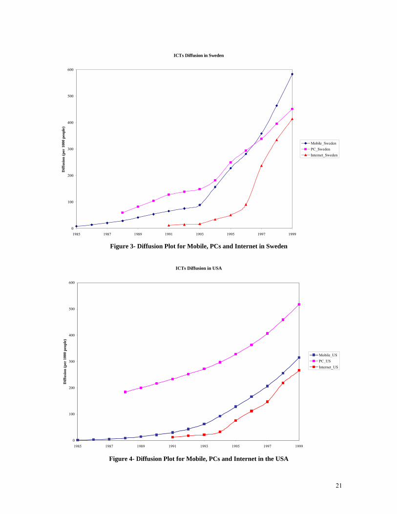
ICTs Diffusion in Sweden

0

100

200

300

400

500

600

1985 1987 1989 1991 1993 1995 1997 1999

Diff

usio

n (p

er 1

000

peop

le)

Mobile_SwedenPC_SwedenInternet_Sweden

Figure 3- Diffusion Plot for Mobile, PCs and Internet in Sweden

ICTs Diffusion in USA

0

100

200

300

400

500

600

1985 1987 1989 1991 1993 1995 1997 1999

Diff

usio

n (p

er 1

000

peop

le)

Mobile_USPC_USInternet_US

Figure 4- Diffusion Plot for Mobile, PCs and Internet in the USA