Download this - Bilingual Publishing Co

Editor-in-ChiefDr. Chin-Ling Chen

Chaoyang University of Technology, Taiwan

Editorial Board Members

Chong Huang, United StatesYoshifumi Manabe, Japan

Hao Xu, United StatesShicheng Guo, United States

Leila Ghabeli, IranDiego Real Mañez, Spain

Senthil Kumar Kumaraswamy, IndiaSanthan Kumar Cherukuri, India

Asit Kumar Gain, AustraliaJue-Sam Chou, Taiwan

Sedigheh Ghofrani, IranYu Tao, China

Lianggui Liu, ChinaVandana Roy, India

Jun Zhu, ChinaZulkifli Bin Mohd Rosli, Malaysia

Radu Emanuil Petruse, RomaniaSaima Saddiq, Pakistan

Saleh Mobayen, IranAsaf Tolga Ulgen, Turkey

Xue-Jun Xie, ChinaMehmet Hacibeyoglu, Turkey

Prince Winston D, IndiaPing Ding, China

Youqiao Ma, CanadaMarlon Mauricio Hernandez Cely, Brazil

Amirali Abbasi, IranGe Song, United States

Rui Min, ChinaP. D. Sahare, India

Volodymyr Gennadievich Skobelev, UkraineHui Chen, China

M.M. Kamruzzaman, BangladeshSeyed Saeid Moosavi Anchehpoli, Iran

Sayed Alireza Sadrossadat, IranFa Wang, United States

Tingting Zhao, ChinaSasmita Mohapatra, India

Akram Sheikhi, Iran

Husam Abduldaem Mohammed, IraqMuhammet Nuri Seyman, TurkeyNeelamadhab Padhy, IndiaAli Mohsen Zadeh, IranOye Nathaniel David, NigeriaXiru Wu, ChinaYashar Hashemi, IranAli Ranjbaran, IranAbdul Qayyum, FranceAlberto Huertas Celdran, IrelandMaxim A. Dulebenets, United StatesYanxiang Zhang, ChinaAlex Michailovich Asavin, Russian FederationJafar Ramadhan Mohammed, IraqShitharth Selvarajan, IndiaSchekeb Fateh, SwitzerlandAlexandre Jean Rene Serres, BrazilDadmehr Rahbari, IranJunxuan Zhao, United StatesJun Shen, ChinaXinggang Yan, United KingdomYuan Tian, ChinaAbdollah Doosti-Aref, IranMingxiong Zhao, ChinaHamed Abdollahzadeh, IranFalu Weng, ChinaWaleed Saad Hilmy, EgyptQilei Li, ChinaQuang Ngoc Nguyen, JapanFei Wang, ChinaXiaofeng Yuan, China Vahdat Nazerian, IranYanling Wei, BelgiumKamarulzaman Kamarudin, MalaysiaTajudeen Olawale Olasupo, United StatesMd. Mahbubur Rahman, KoreaIgor Simplice Mokem Fokou, CameroonHéctor F. Migallón, SpainNing Cai, China

Dr. Chin-Ling ChenEditor-in-Chief

Journal ofElectronic & Information

Systems

Volume 1 Issue 2 · Octobe 2020 · ISSN 2661-3204 (Online)

Volume 1 | Issue 2 | Octobe 2019 | Page 1-25Journal of Electronic & Information Systems

Contents

CopyrightJournal of Electronic & Information Systems is licensed under a Creative Commons-Non-Commercial 4.0 International Copyright (CC BY- NC4.0). Readers shall have the right to copy and distribute articles in this journal in any form in any medium, and may also modify, convert or create on the basis of articles. In sharing and using articles in this journal, the user must indicate the author and source, and mark the changes made in articles. Copyright © BILINGUAL PUBLISH-ING CO. All Rights Reserved.

Empirical Wavelet Transform; Stationary and Nonstationary Signals

Hesam Akbari Sedigheh Ghofrani

Increase the Quality of Life through the Development of Automation

Anoushe Arab

The Experimental WSN Network for Underground Monitoring H2 Abundance in the Mine

Atmosphere Karnasurt Mine Lovozero Layered Alkaline Intrusion

Asavin A. M. Puha V.V. Baskakov S.S. Chesalova E.I. Litvinov A.V.

Three Median Relations of Target Azimuth in one Dimensional Equidistant Double Array

Tao Yu

Article

1

6

15

21

1

Journal of Electronic & Information Systems | Volume 01 | Issue 02 | October 2019

Distributed under creative commons license 4.0 DOI: https://doi.org/10.30564/jeisr.v1i2.1008

Journal of Electronic & Information Systems

https://ojs.bilpublishing.com/index.php/jeis

ARTICLE

Empirical Wavelet Transform; Stationary and Nonstationary Signals

Hesam Akbari1　Sedigheh Ghofrani2* 1. Biomedical Engineering Department, South Tehran Branch, Islamic Azad University, Tehran, Iran 2. Electrical Engineering Department, South Tehran Branch, Islamic Azad University, Tehran, Iran

ARTICLE INFO ABSTRACT

Article historyReceived: 9 July 2019 Accepted: 4 November 2019Published Online: 31 March 2020

Signal decomposition into the frequency components is one of the oldest challenges in the digital signal processing. In early nineteenth century, Fourier transform (FT) showed that any applicable signal can be decom-posed by unlimited sinusoids. However, the relationship between time and frequency is lost under using FT. According to many researches for appropriate time-frequency representation, in early twentieth century, wavelet transform (WT) was proposed. WT is a well-known method which developed in order to decompose a signal into frequency compo-nents. In contrast with original WT which is not adaptive according to the input signal, empirical wavelet transform (EWT) was proposed. In this paper, the performance of discrete WT (DWT) and EWT in terms of signal decomposing into basic components are compared. For this pur-pose, a stationary signal including five sinusoids and ECG as biomedical and nonstationary signal are used. Due to being non-adaptive, DWT may remove signal components but EWT because of being adaptive is appro-priate. EWT can also extract the baseline of ECG signal easier than DWT.

Keywords:Empirical wavelet transformDiscrete wavelet transformSignal decomposition

　

*Corresponding Author:Sedigheh Ghofrani,Electrical Engineering Department, South Tehran Branch, Islamic Azad University, Tehran, Iran;Email: [email protected]

1. Introduction

Signal decomposition into the frequency compo-nents is one of the oldest challenges in the digital signal processing. In early nineteenth century,

Fourier transform (FT) showed that any applicable signal can be decomposed by unlimited sinusoids. Moreover, the relationship between time and frequency is lost in FT. In order to overcome the mentioned problem, short time Fourier transform (STFT) was proposed, where a signal is windowed in time domain and the FT is individually com-puted for each window. Through this, the signal spectrum corresponding to every window is obtained separately. Although using STFT preserves the time-frequency rela-tionship, and it is known as a time-frequency representa-

tion, increasing the width of used window is equivalent to decrease the time resolution [1]. Since basis functions of both FT and the STFT are in exponential form, under no similarity between the signal and the exponential element function, the resultant frequency spectrum cannot offer an appropriate representation about the signal frequency components. In early twentieth century, according to many researches for appropriate time-frequency representation, wavelet transform (WT) was proposed [2]. As, the mother wavelet is not necessarily exponential, it can be used for time-frequency analysis of those signals which are not combinations of exponential functions. The first basis function proposed for the WT called Haar [3], different ba-sis functions as Little-Paley [4], Meyer [5], and Daubechies [1] were proposed.

2


Distributed under creative commons license 4.0

Although, many advantages of WT as a time-frequency decomposition method is known, the bottle neck of using wavelet is nonadaptivity to the input signal. So empirical mode decomposition (EMD) which operates adaptively according to the input signal was proposed [6]. In general, EMD decomposes a signal to different intrinsic mode functions (IMFs). It is a reversible operation that means sum of obtained IMFs and the residual signal synthesize the original input signal. Although, EMD algorithm has primarily been considered in several signal processing applications, lack of closed-form mathematical expres-sion, time consuming, and also sensitivity to the noise are always known as its limitation factors.

In 2013, an approach called empirical wavelet trans-form (EWT) was proposed to overcome the mentioned drawbacks [7]. EWT is adaptive similar to EMD but instead of EMD, it is not noise sensitive. Also, having a mathe-matical expression, capable EWT to analyze signals faster than EMD. Comparison among EMD, EWT and discrete WT (DWT) as a well-known non adaptive time-frequency signal representation were reported [8-10]. In this paper, as a case study of processing a stationary signal and also ECG as a nonstationary signal, we compare the performance of the DWT and EWT as well.

The paper is organized as follows. In Section 2, the the-ory of original WT and EWT are explained. Then in Sec-tion 3, two signals are decomposed by EWT and DWT. Finally, both decomposition algorithms are evaluated. The paper conclusion is given in Section 4.

2. WT And EWT

In general, WT by using the filter bank decomposes a signal into specified frequency sub-bands. The cut-off frequency of the filter bank at the first and the second decomposition level, are 2/π and 4/π in order, so it is

n2/π at the nth decomposing level. In other word, for the nth decomposition level, the bandwidth of low-pass filter is [0, n2/π ] and the bandwidth of high-pass filter is [ n2/πfalse, 12/ −nπ ]. Two functions called Φ as scaling function (SF) and Ψ as wavelet function (WF) have key roles in signal decomposition,

otherwise 0

1t0 if 1(t)

<≤

=Φ (1)

<≤−

<≤=Ψ

otherwise 01t/21 if 12/1t0 if 1

)t( (2)

DOI: https://doi.org/10.30564/jeisr.v1i2.1008

For every decomposition level, the signal projection with low-pass filter and high-pass filter are called approx-imation and detail. However, the cut-off frequencies in WT for all decomposition levels are constant that means the WT is not adaptive to the input signal. In contrast, for EWT, the filter bank cut-off frequencies are not con-stant and vary according to the input signal components [7]. Using FT, the frequency spectrum of the input signal is obtained in [0, 𝜋] and the local maxima of frequency spectrum are marked, and then midpoints of every pair maximum are used as the filter bank cut-off frequency. It should be noted that the number of required local max-ima depends on the number of decomposition levels. In other words n largest local maximums are required for n decomposition levels, also the first cut-off frequency falls between zero and the maximum at the lowest frequency. After specifying the cut-off frequencies, the filter bank is formed according to the idea of Littlewood–Paley and Meyers wavelets [11]. For EWT, the SF and the WF func-tions are defined in Fourier domain as [7],

φ ω λ ω ω λ ω ( ) cos( ) if (1- ) | | (1 ) f f = ≤ ≤ +

πβ λ ω1 if| | (1- )

0 otherwise

( , )2

1

ω λ ω

1 1

f ≤ 1

(3)

ψ ωi n f=2,.., ( ) =

cos( ) if (1 ) | | (1- )

sin( ) if (1 ) | | (1 )

πβ λ ω

πβ λ ω

( , )1 if (1 ) | | (1- )

0 otherwise

( , )2

2i

i

+1 − ≤ ≤

+ ≤ ≤

+ ≤ ≤ +

λ ω ω λ ω

λ ω ω λ ω

λ ω ω λ ω

1 1i f i

1

+ +

i f i

i f i

+

(4)

where,

β λ ω β( , ) ( ) i =| | (1 )ω λ ωf i− −

2λωi

(5)

where ,..,,21,..2,1 ncutcutcutni fff==ω and )(min ë

i 1i

i 1i

ωωωω

+−

<−

+

which make sure the EWT coefficient are in )(2 ℜL space,

and )(yβ is,

β β β( ) ( ) (1 ) 1 y [0,1]y y y= + − = ∀ ∈ 1 if y 1

0 if y 0≤

≥ (6)

Similar to WT, approximation and detail coefficients are obtained by using the inner product between the input signal and SF and WF, respectively.

3



3. Simulation Result

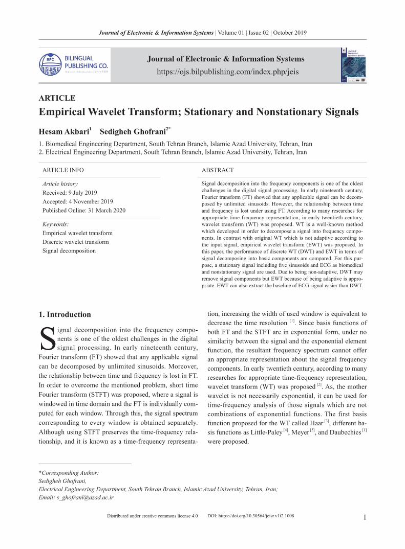
In order to demonstrate the capability of EWT, in com-parison with DWT based on Dubeches, a stationary sig-nal and ECG signal are used. The first signal )t(x is an stationary and multicomponent consists of five sinusoids with different amplitudes and frequencies as,

)t(x)t(x)t(x)t(x)t(x)t(x 54321 ++++= (7)

where x1(t) 4sin(4 t)= π , x2 (t) 13sin(16 t)= − π ,x3 (t) 11sin(40 t)= π , x4 (t) 8sin(64 t)= − π and ) t128sin(5)t(5 π=x . According to the frequency com-

ponents of signal )t(x , the sampling frequency is consid-ered 256 Hz. The signal )t(x is decomposed by wavelet with 4 decomposition levels and EWT considering 5 sub-bands, see Figure1. As mentioned before and observed in Figure1-a, the bandwidth of filter banks for WT are fixed; that means if any frequency component of the input signal lay on the cut-off frequency of filter bank, it is removed. For the signal )t(x , it happened for the second, fourth and fifth components with frequencies equal 8, 32, and 64 Hz. As shown in Figure1-b, signal decomposition by EWT, at first the frequency spectrum of )t(x is obtained in [0,], then local maximums are specified, and accordingly the

Figure 1. Decomposing the signal x(t), Eq(7), by (a) WT, (b) EWT

4



cut-off frequencies of filter bank are determined. It should be noted that the first cut-off frequency lies between zero and the first maximum with the lowest frequency. All sig-nals in nature have higher amplitude in lower frequencies compared to high frequencies, in addition a large amount of information exists in lower frequencies where high fre-

quencies include noise. According to the explained EWT methodology, the most of EWT sub bands are chosen in low frequencies

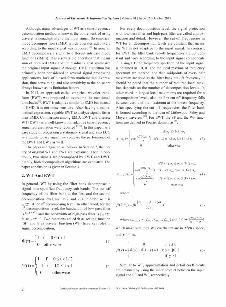
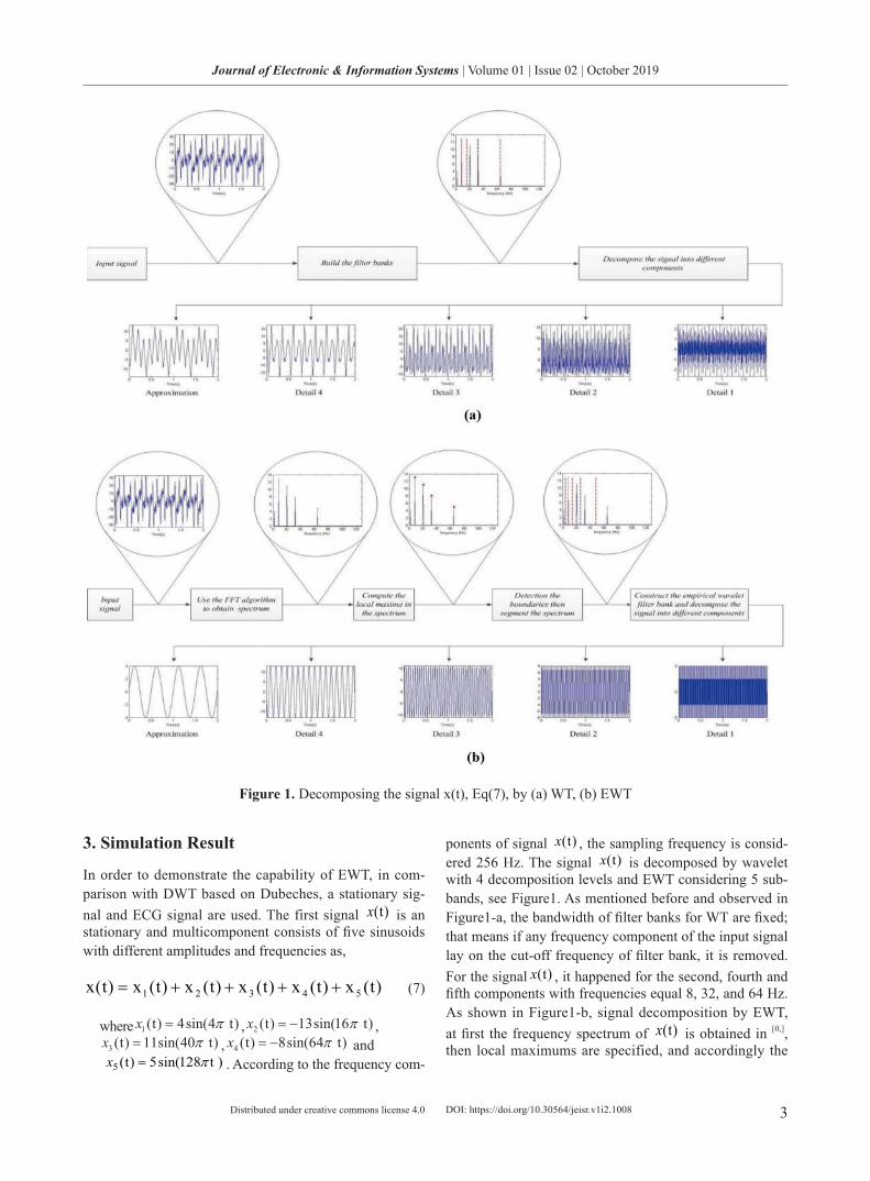
In WT, as the sampling frequency increases, the num-ber of decomposition level is increased in order to be capable of investigating the low frequency components

Figure 2. Decomposing ECG signal and extracting the baseline by (a) WT, (b) EWT


5



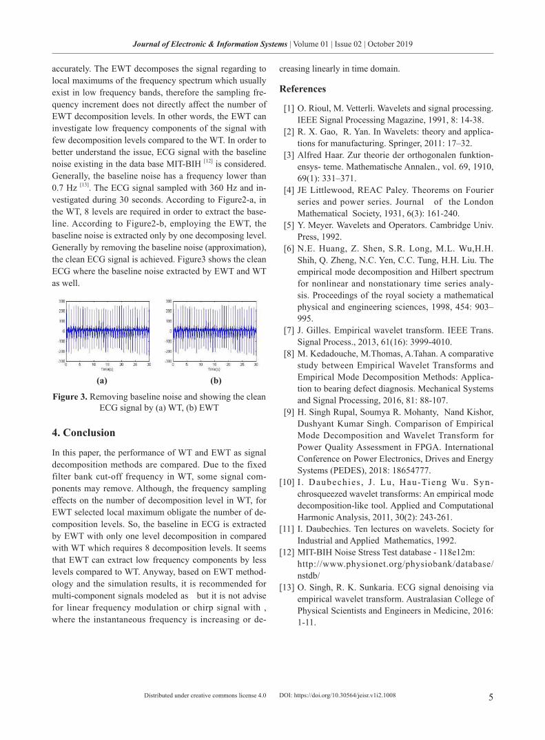
accurately. The EWT decomposes the signal regarding to local maximums of the frequency spectrum which usually exist in low frequency bands, therefore the sampling fre-quency increment does not directly affect the number of EWT decomposition levels. In other words, the EWT can investigate low frequency components of the signal with few decomposition levels compared to the WT. In order to better understand the issue, ECG signal with the baseline noise existing in the data base MIT-BIH [12] is considered. Generally, the baseline noise has a frequency lower than 0.7 Hz [13]. The ECG signal sampled with 360 Hz and in-vestigated during 30 seconds. According to Figure2-a, in the WT, 8 levels are required in order to extract the base-line. According to Figure2-b, employing the EWT, the baseline noise is extracted only by one decomposing level. Generally by removing the baseline noise (approximation), the clean ECG signal is achieved. Figure3 shows the clean ECG where the baseline noise extracted by EWT and WT as well.

(a) (b)

Figure 3. Removing baseline noise and showing the clean ECG signal by (a) WT, (b) EWT

4. Conclusion

In this paper, the performance of WT and EWT as signal decomposition methods are compared. Due to the fixed filter bank cut-off frequency in WT, some signal com-ponents may remove. Although, the frequency sampling effects on the number of decomposition level in WT, for EWT selected local maximum obligate the number of de-composition levels. So, the baseline in ECG is extracted by EWT with only one level decomposition in compared with WT which requires 8 decomposition levels. It seems that EWT can extract low frequency components by less levels compared to WT. Anyway, based on EWT method-ology and the simulation results, it is recommended for multi-component signals modeled as but it is not advise for linear frequency modulation or chirp signal with , where the instantaneous frequency is increasing or de-

creasing linearly in time domain.

References

[1] O. Rioul, M. Vetterli. Wavelets and signal processing. IEEE Signal Processing Magazine, 1991, 8: 14-38.

[2] R. X. Gao, R. Yan. In Wavelets: theory and applica-tions for manufacturing. Springer, 2011: 17–32.

[3] Alfred Haar. Zur theorie der orthogonalen funktion-ensys- teme. Mathematische Annalen., vol. 69, 1910, 69(1): 331–371.

[4] JE Littlewood, REAC Paley. Theorems on Fourier series and power series. Journal of the London Mathematical Society, 1931, 6(3): 161-240.

[5] Y. Meyer. Wavelets and Operators. Cambridge Univ. Press, 1992.

[6] N.E. Huang, Z. Shen, S.R. Long, M.L. Wu,H.H. Shih, Q. Zheng, N.C. Yen, C.C. Tung, H.H. Liu. The empirical mode decomposition and Hilbert spectrum for nonlinear and nonstationary time series analy-sis. Proceedings of the royal society a mathematical physical and engineering sciences, 1998, 454: 903–995.

[7] J. Gilles. Empirical wavelet transform. IEEE Trans. Signal Process., 2013, 61(16): 3999-4010.

[8] M. Kedadouche, M.Thomas, A.Tahan. A comparative study between Empirical Wavelet Transforms and Empirical Mode Decomposition Methods: Applica-tion to bearing defect diagnosis. Mechanical Systems and Signal Processing, 2016, 81: 88-107.

[9] H. Singh Rupal, Soumya R. Mohanty, Nand Kishor, Dushyant Kumar Singh. Comparison of Empirical Mode Decomposition and Wavelet Transform for Power Quality Assessment in FPGA. International Conference on Power Electronics, Drives and Energy Systems (PEDES), 2018: 18654777.

[10] I . Daubechies , J . Lu, Hau-Tieng Wu. Syn-chrosqueezed wavelet transforms: An empirical mode decomposition-like tool. Applied and Computational Harmonic Analysis, 2011, 30(2): 243-261.

[11] I. Daubechies. Ten lectures on wavelets. Society for Industrial and Applied Mathematics, 1992.

[12] MIT-BIH Noise Stress Test database - 118e12m: http://www.physionet.org/physiobank/database/

nstdb/ [13] O. Singh, R. K. Sunkaria. ECG signal denoising via

empirical wavelet transform. Australasian College of Physical Scientists and Engineers in Medicine, 2016: 1-11.


6





ARTICLE

Increase the Quality of Life through the Development of Automation

Anoushe Arab*

Education office of Zahedan, Iran


Article historyReceived: 31 October 2019Accepted: 30 January 2020Published Online: 31 March 2020

This paper discusses needs for the automation of the underdevelopment communities. The novelty of this research is the link between production of microprocessors and increasing of the life quality. This study high-lights the importance of efficient and economic architecture of logical cir-cuits for the automation. The aim of this research is to produce a logical circuit, which includes suitable gates. The circuit will be embedded in the automatic devices as a microprocessor to cause programmed functions. This research reports analytically a workshop method to build the circuit. It uses an assembly card and required gates. Then, it suggests certain VHDL codes to drive a motor. The workshop presents the configuration schemes and connection board for every gate. In addition, it shows a schematic wiring diagram of the circuit. Finally, the economic analysis proves the mass production of the circuit will enhance the automation and consequently the quality of life. The outcome of this research is a helpful experience to the engineers, manufacturers and students of the relevant disciplines to resolve the inequality in the use of the modern technologies.

Keywords:Logic circuitsDigital gatesMicroprocessorsMass productionQuality of lifeAssembly card

　

*Corresponding Author:Anoushe Arab,Education office of Zahedan, Iran;Email: [email protected]

1. Introduction

During the recent decades an exciting evolution in the capabilities of microprocessors has been seen. The rapid spread of microprocessors in the

daily life increased the necessity of embedding a micro-processor somewhere inside the machineries and tools. The advent of digital and automatization technologies for urban infrastructure, residential buildings and other urban spaces has increased the need for more inexpensive and functional logical circuits. Therefore, as today’s urban life is becoming increasingly automated, great demands are placed on the logical circuits and microprocessors we use in the buildings, components of urban infrastructures such as automatic doors, automatic tellers, home security and control, bus and train ticket seller machines and so on.

With some simple keystrokes as the only input, we expect the automated device to handle the rest to achieve the de-sired result.

The main question addressed by this paper is how shall we improve the quality of life in the underdevelopment communities with the help of automatization? Therefore the question is, how shall we produce a more efficient, economic and purposeful digital circuit for controlling a DC motor with special functional requirements?

The goal is to encourage regional/urban planners and entrepreneurs in the underdevelopment cities to increase the quality of urban life by emphasizing on digitalizing and au-tomatizing of the urban life. For this reason, the aim of this research is to design and manufacture a more efficient and economic logical circuit card and microprocessor for digital control of DC motors via simple analog joysticks.

7



The method of this research paper to achieve the goal has both theoretical and experimental bulks. Neverthe-less, it has been given a lot of importance to report a workshop experience to produce a logical circuit.

This paper is structured in 5 parts as follows: Intro-duction, theoretical explorations, workshop experiences, methodology and discussions, and conclusions.

2. Theoretical Explorations

Human beings always use knowledge and technology to make their lives more comfortable. As far as societies rely more on knowledge, technology and fairness, they have been able to create a better quality of life. [22]. As today’s society is becoming increasingly automated, great demands are placed on the products we use for a more qualified and comfortable life [6,8]. During doing a lot of things such simple individual issues, professional tasks or making decisions about the important and complex problems, we expect immediate assistance via automatic devices and tools [7,11,17]. With some simple keystrokes as the only input, we expect the automation to handle the rest to achieve the desired result [9,15,16]. Scholars have explored the link between progress in knowledge-based urban planning and improvement of urban life quality [10,26]. There have been several attempts to build small-size and lightweight microprocessors with simple logical circuits. The purpose has always been making things easy and ac-curate. This purpose consequently has improved human life quality [24]. Scientists believe that a characteristic of our era, which is the result of exploiting the achievements of the industrial revolution, is the spread of the digitaliza-tion and automatization technologies. On the other word in the new era, people use the automated tools in more circumstances. The industrial revolution changed the tools of manual labor, relied on the power of human beings into mechanical instruments and motors. Whereas the advanc-es in the digital and automatic technologies change the mechanical instruments to automatic, light, small, effi-cient, inexpensive, and comfortable tools and motors [28]. Although it was expected that the advances in digitization and automatization would serve all human beings, regard-less their geographical situations, this did not happen. Comparing countries with each other and even comparing the cities of a certain country with each other, especially in the underdevelopment countries, shows that the use of automation achievements is not equivalent. As a result, people in the underdevelopment cities and regions do not enjoy the benefits of automatic progress and their quality of life is less than minimum standards and sometimes unacceptable [23]. For these reasons, the necessity of the importing knowledge and technology for the production

of logical circuits and microprocessors in all countries is understood [14]. At the same time, we know that any microprocessor-based system necessarily has some stan-dard elements and gates such as memory, timing, input/output (I/O), analog to digital (A/D) converter, registers, resistors, diodes, interrupter, etc. [2]. Engineers and man-ufacturers of this industry, i.e. Baker and Allan et al have been researching on this subject and addressed the char-acteristics of gates and components that form a logical circuit [1,5]. Also, the standards and qualities necessary for the production of gates and components of logical circuits are the subject of research and analysis of numerous engi-neers and manufacturers. For example, Auch and Wright believe that major researches on the logical circuits have been carried out from a manufacturing standpoint, which considers less improvement of the productions [3,27]. From the practical point of view, we are facing always with this question: How shall gates and components of a logical cir-cuit be interconnected and assembled to provide reliable services to users? Many engineers in different manufac-turing companies, i.e. Patterson & Sequin have explored the right answers to the above question. They thought that it would be possible to put numerous electronic gates onto a single chip. They discussed the desirable architectural features in modem microprocessors. They concluded that: “a processor design includes features such as an on-chip memory hierarchy, multiple homogeneous caches for en-hanced execution parallelism, support for complex data structures and high-level languages, a flexible instruction set, and communication hardware” [18]. A microprocessor needs an engine to work. An engine can be controlled digitally, analogously, or so-called mechanistic. The ad-vantage of digital control is the ability to pre-program movements and control schemes. This makes it fast, pre-cise and the movements can be repeated exactly the same way thousands of times a day. Another advantage of using a microprocessor for motor control is that communication of the motor control and the rest of the process takes place via the data bus already in the microprocessor. Analog control does not require advanced equipment. This option fits well when the steering does not need to follow prede-termined schedules. Furthermore, we think on how shall the progress made in the manufacturing industry of logical circuits and microprocessors be used to serve the automa-tion of the underdevelopment regions? The right answer to this question is important, particularly when scholars suggest the use of microprocessors to resolve the critical problems, i.e. the water crisis in the underdevelopment re-gions [22]. The production of standard electronic gateways and the assembly of those in digital circuits in the form of smaller, lighter, cheaper and more functional microproces-

8



sors are the core attempts of the engineers and investors in this industry. Only as one sample see the research has been done by Paul and colleagues. They reported that: “Workshop participants consistently called for the ad-vancement of the components and interconnects required for developing smart goods. Persistent themes included reduced power, enhanced battery life, energy harvesting, smaller sizes, and lower cost” [19]. We reviewed the opin-ions and experiences of engineers and manufacturers of logical circuits. We reviewed four issues, namely 1- the standards and quality of digital gateways, 2- components and gateways included in a logical circuit, 3- optimal connection and efficient assembly of components in a cir-cuit, 4- and the optimal production of gates and micropro-cessors. According to this review, in the next section, we are going to analyze a workshop experience for generating a digital logic circuit for a microprocessor.

3. Workshop Experiences

3.1 Digital Control for DC Motor

This workshop experience is about the design of a circuit board for digital control of a small DC motor. The expe-rience contains solutions, connection tables, assembly diagrams and descriptions of selected components. An economic calculation of 100 circuits is performed to prove the profitability of microprocessors’ mass production in the underdevelopment regions. In addition, we developed program codes for programmable logic devices, PLD-cir-cuits, and test programs. In the other words, the workshop experience aimed at designing and manufacturing an elec-tronic card for digital control of a DC motor via a simple analog joystick. An automated system has an engine as an actuator. Control of the motor can be done in different ways, but we will concentrate on the procedure of digital control. This type of control has become very common and in this workshop we would use a standard processor, a digital standard circuit with required gates and a con-trolling principle. Solution methods have been chosen on the basis of the knowledge that we have acquired through the theoretical explorations and exercises in the subject areas. We should develop and realize a solution for con-trolling the DC motor with special functional require-ments. The targets of the workshop were as follows:

(1) Design and improvement of a system that is in ac-cordance with a given specification of requirements

(2) Different conversion principles for A/D and D/A converters and its performance

(3) Breaking down the problem into minor sub-prob-lems and dividing our suggested electronic system into functional blocks

(4) Design principles for the testability of the systemIn addition, the control specifications were:(1) The control is available with analog joystick deliv-

ers voltages between 0 and 5 V.(2) The joystick position should directly affect the en-

gine speed with the following setups:① Neutral position: stationary motor② Maximum position: Maximum speed in clockwise

rotation ③ Minimum position: Maximum speed in counter-

clockwise rotation(3) The control card must be able to be connected to

EXKIT as an interface between the microprocessor and the engine

(4) At low speeds, the engine should rotate without snatching.

(5) The joystick position should be presented on the display.

(6) The cost of component never exceeds 25 US$.(7) The control card should be easy to troubleshoot and

repair.(8) Software for testing motor control or joystick mode

must be produced.(9) The documentation must be able to be used by tech-

nicians for further production as well as by the engineer for the improvement or modification of the design

(10) Calculation basis for planned production of 100 units

3.2 Design of the Required Digital Circuit

The Following figure exhibits the block diagram of our proposed circuit with the applied gates and components.

Computer↔Interface→Converter→Joystick

↓↓

InterfaceDisplay

↓

PWM

↓

Motor

Figure 1. Flowchart of the gates included in the circuit block

Following we describe every component in terms of its characteristics, functions, and connections schema.

JoystickThe joystick consists of two potentiometers, of which only

one is used. The potentiometer is an adjustable resistor whose value changes depending on the position of the joystick.

Circuit ADC0804In order to convert the analog signal from the joystick to


9



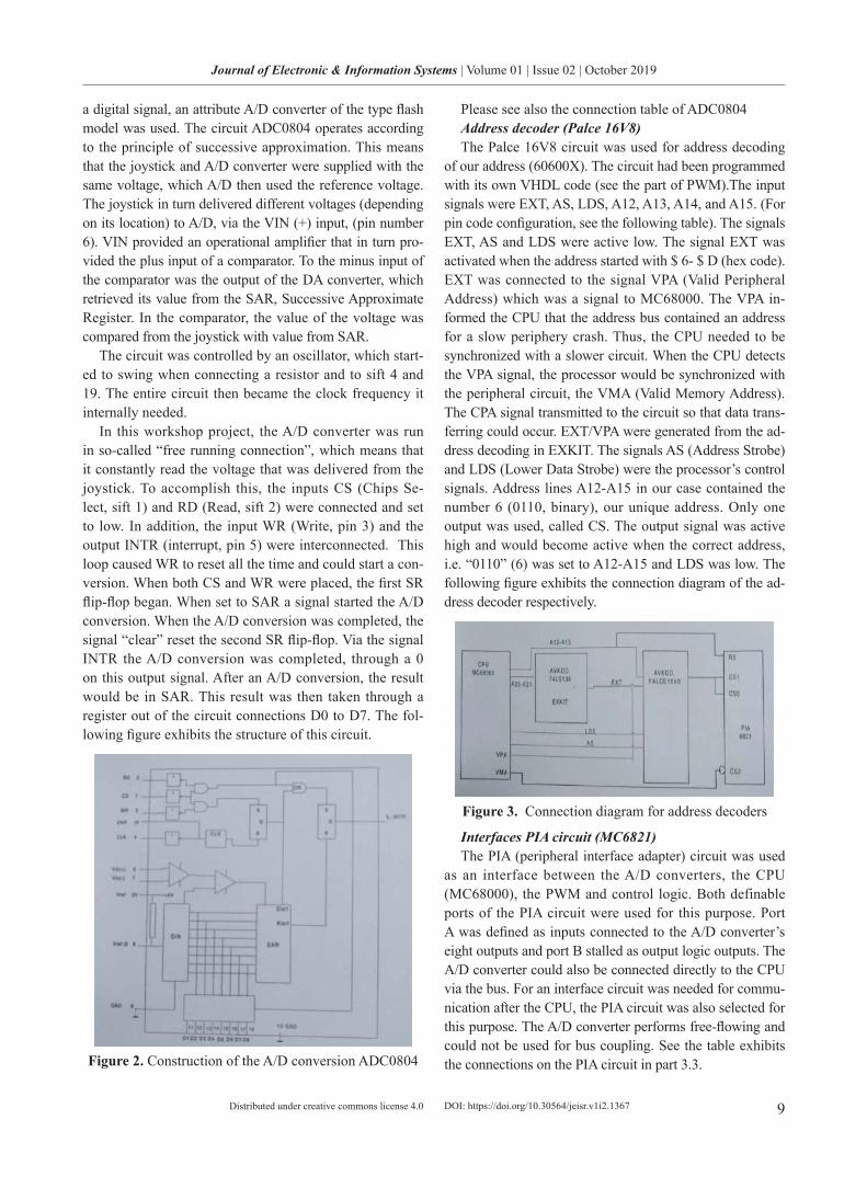
a digital signal, an attribute A/D converter of the type flash model was used. The circuit ADC0804 operates according to the principle of successive approximation. This means that the joystick and A/D converter were supplied with the same voltage, which A/D then used the reference voltage. The joystick in turn delivered different voltages (depending on its location) to A/D, via the VIN (+) input, (pin number 6). VIN provided an operational amplifier that in turn pro-vided the plus input of a comparator. To the minus input of the comparator was the output of the DA converter, which retrieved its value from the SAR, Successive Approximate Register. In the comparator, the value of the voltage was compared from the joystick with value from SAR.

The circuit was controlled by an oscillator, which start-ed to swing when connecting a resistor and to sift 4 and 19. The entire circuit then became the clock frequency it internally needed.

In this workshop project, the A/D converter was run in so-called “free running connection”, which means that it constantly read the voltage that was delivered from the joystick. To accomplish this, the inputs CS (Chips Se-lect, sift 1) and RD (Read, sift 2) were connected and set to low. In addition, the input WR (Write, pin 3) and the output INTR (interrupt, pin 5) were interconnected. This loop caused WR to reset all the time and could start a con-version. When both CS and WR were placed, the first SR flip-flop began. When set to SAR a signal started the A/D conversion. When the A/D conversion was completed, the signal “clear” reset the second SR flip-flop. Via the signal INTR the A/D conversion was completed, through a 0 on this output signal. After an A/D conversion, the result would be in SAR. This result was then taken through a register out of the circuit connections D0 to D7. The fol-lowing figure exhibits the structure of this circuit.

Figure 2. Construction of the A/D conversion ADC0804

Please see also the connection table of ADC0804Address decoder (Palce 16V8)The Palce 16V8 circuit was used for address decoding

of our address (60600X). The circuit had been programmed with its own VHDL code (see the part of PWM).The input signals were EXT, AS, LDS, A12, A13, A14, and A15. (For pin code configuration, see the following table). The signals EXT, AS and LDS were active low. The signal EXT was activated when the address started with $ 6- $ D (hex code). EXT was connected to the signal VPA (Valid Peripheral Address) which was a signal to MC68000. The VPA in-formed the CPU that the address bus contained an address for a slow periphery crash. Thus, the CPU needed to be synchronized with a slower circuit. When the CPU detects the VPA signal, the processor would be synchronized with the peripheral circuit, the VMA (Valid Memory Address). The CPA signal transmitted to the circuit so that data trans-ferring could occur. EXT/VPA were generated from the ad-dress decoding in EXKIT. The signals AS (Address Strobe) and LDS (Lower Data Strobe) were the processor’s control signals. Address lines A12-A15 in our case contained the number 6 (0110, binary), our unique address. Only one output was used, called CS. The output signal was active high and would become active when the correct address, i.e. “0110” (6) was set to A12-A15 and LDS was low. The following figure exhibits the connection diagram of the ad-dress decoder respectively.

Figure 3. Connection diagram for address decoders

Interfaces PIA circuit (MC6821)The PIA (peripheral interface adapter) circuit was used

as an interface between the A/D converters, the CPU (MC68000), the PWM and control logic. Both definable ports of the PIA circuit were used for this purpose. Port A was defined as inputs connected to the A/D converter’s eight outputs and port B stalled as output logic outputs. The A/D converter could also be connected directly to the CPU via the bus. For an interface circuit was needed for commu-nication after the CPU, the PIA circuit was also selected for this purpose. The A/D converter performs free-flowing and could not be used for bus coupling. See the table exhibits the connections on the PIA circuit in part 3.3.


10



Light signals for joystick modeVisual presentation of the motor’s direction and speed

was solved with LEDs and a programmed logic circuit. To mark the engine speed and direction and thus the joystick position, a Palce 22V10 PLD circuit was programmed. By defining the output signals from the A/D converter into in-put signals and dividing them into 10 intervals of total 256 combinations, the PLD circuit delivered 10 output signals coupled to an active low LED (B1001H) protected by the 220 Ω resistor. The PLD circuit was programmed to shine with all the diodes when the joystick was in a neutral po-sition. At maximum speed in each direction, half of the diodes were switched off on the corresponding side of the ramp and vice versa. The following table exhibits the con-figuration order of the diode.

PWM - Palce 16V8 (NAND)Since we chose to extract the maximum signal from the

counter outputs ( ) and all inputs are high (225), we had to connect the wires via a NAND gate to deliver a low signal. This was solved with the following VHDL code.

If (10=‘1’ and 11=‘1’ and 12=‘1’ and 13=‘1’ and 14=‘1’ and 15=‘1’ and

16=‘1’ and 17=‘1’) then max≤‘0’;Else max≤‘1’;End if;We ignore here to write the full-VHDL code. The count-

er we used (SN74HC590) had RCO value that was ahead of the outputs. If we were to use the RCO signal from the counter, we would not be able to extract the maximum val-ue from the counter. To be able to use the maximum value from the counter, we had an 8-input NAND gate. By using the outputs from the counter to the inputs of the NAND gate, we got the maximum value. The following figure ex-hibits the configuration scheme of our NAND gate.

Figure 4 . Configuration scheme of the NAND gate

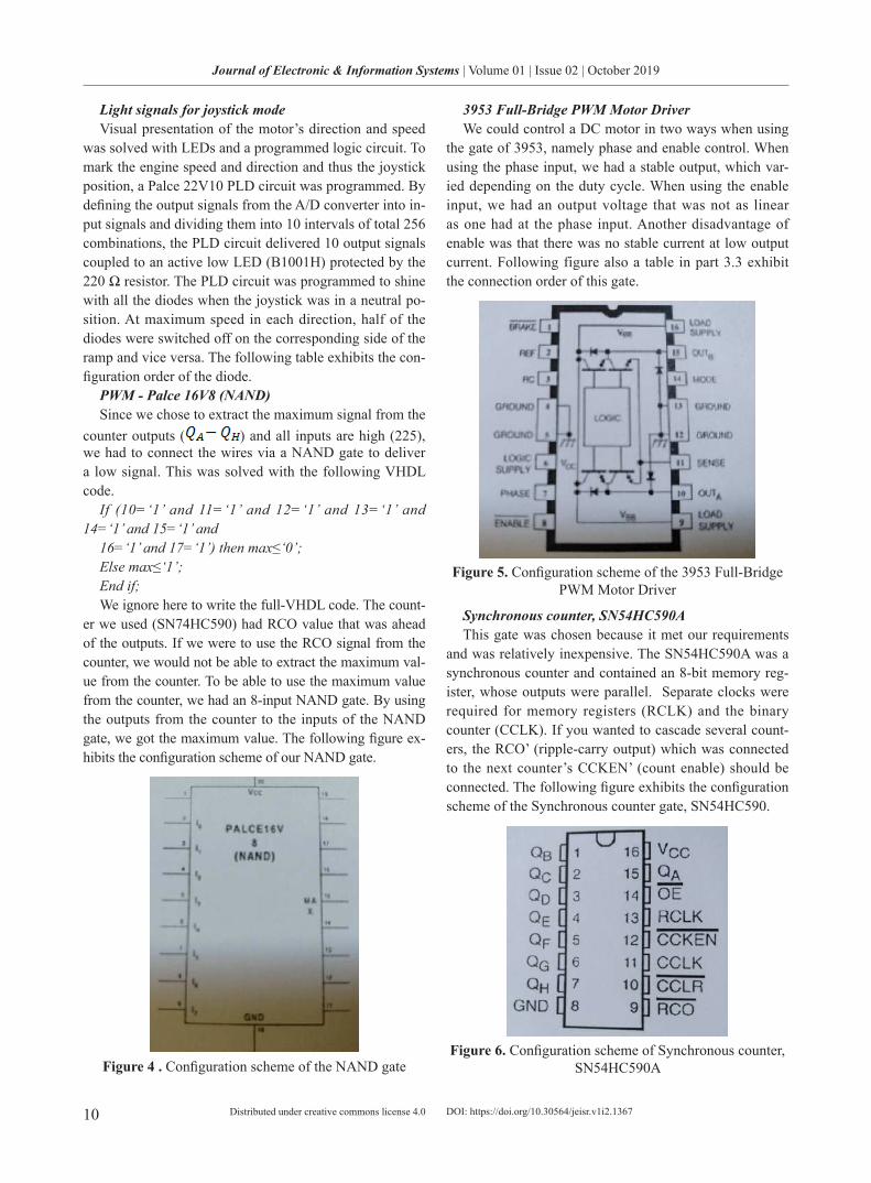
3953 Full-Bridge PWM Motor DriverWe could control a DC motor in two ways when using

the gate of 3953, namely phase and enable control. When using the phase input, we had a stable output, which var-ied depending on the duty cycle. When using the enable input, we had an output voltage that was not as linear as one had at the phase input. Another disadvantage of enable was that there was no stable current at low output current. Following figure also a table in part 3.3 exhibit the connection order of this gate.

Figure 5. Configuration scheme of the 3953 Full-Bridge PWM Motor Driver

Synchronous counter, SN54HC590AThis gate was chosen because it met our requirements

and was relatively inexpensive. The SN54HC590A was a synchronous counter and contained an 8-bit memory reg-ister, whose outputs were parallel. Separate clocks were required for memory registers (RCLK) and the binary counter (CCLK). If you wanted to cascade several count-ers, the RCO’ (ripple-carry output) which was connected to the next counter’s CCKEN’ (count enable) should be connected. The following figure exhibits the configuration scheme of the Synchronous counter gate, SN54HC590.

Figure 6. Configuration scheme of Synchronous counter, SN54HC590A


11



An active low signal should be phased out when the counter had finished counting (at 255). We called this the maximum signal. Our solution was that from the outputs ( ) pulled these lines to a PLD made for a NAND gate. The alternative was to remove the maximum signal from RCO directly. The following figure is the map of the connections.

Figure 7. Map of the synchronous counter connecting lines

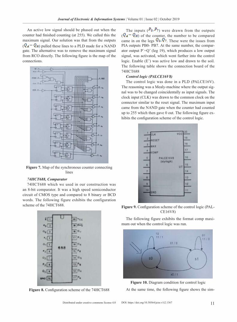
74HCT688, Comparator74HCT688 which we used in our construction was

an 8-bit comparator. It was a high speed semiconductor circuit of CMOS type and compared to 8 binary or BCD words. The following figure exhibits the configuration scheme of the 74HCT688.

Figure 8. Configuration scheme of the 74HCT688

The inputs ( - ) were drawn from the outputs ( ) of the counter, the number to be compared came in on the legs - . These were the issues from PIA outputs PB0- PB7. At the same number, the compar-ator output P´=Q’ (leg 19), which produces a low output signal, was activated, which went further into the control logic. Enable (E’) was active low and drawn to the soil. The following table shows the connection board of the 74HCT688

Control logic (PALCE16V8)The control logic was done in a PLD (PALCE16V).

The reasoning was a Mealy-machine where the output sig-nal was to be changed coincidentally as input signals. The clock input (CLK) was drawn to the common clock on the connector similar to the reset signal. The maximum input came from the NAND gate when the counter had counted up to 255 which then gave 0 out. The following figure ex-hibits the configuration scheme of the control logic.

Figure 9. Configuration scheme of the control logic (PAL-CE16V8)

The following figure exhibits the format comp maxi-mum out when the control logic was run.

Figure 10. Diagram condition for control logic

At the same time, the following figure shows the sim-


12



ulated condition, we supplied with the help of the simula-tor.

Figure 11. Simulation of the control logic of the format: comp max/out

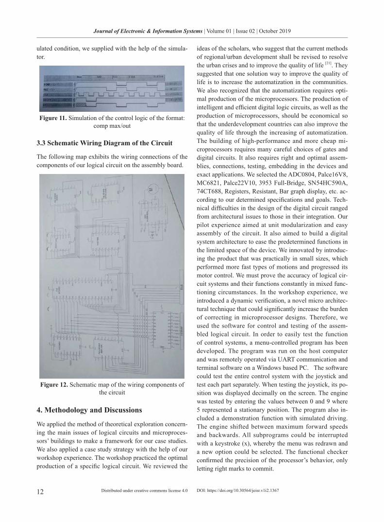
3.3 Schematic Wiring Diagram of the Circuit

The following map exhibits the wiring connections of the components of our logical circuit on the assembly board.

Figure 12. Schematic map of the wiring components of the circuit

4. Methodology and Discussions

We applied the method of theoretical exploration concern-ing the main issues of logical circuits and microproces-sors’ buildings to make a framework for our case studies. We also applied a case study strategy with the help of our workshop experience. The workshop practiced the optimal production of a specific logical circuit. We reviewed the

ideas of the scholars, who suggest that the current methods of regional/urban development shall be revised to resolve the urban crises and to improve the quality of life [21]. They suggested that one solution way to improve the quality of life is to increase the automatization in the communities. We also recognized that the automatization requires opti-mal production of the microprocessors. The production of intelligent and efficient digital logic circuits, as well as the production of microprocessors, should be economical so that the underdevelopment countries can also improve the quality of life through the increasing of automatization. The building of high-performance and more cheap mi-croprocessors requires many careful choices of gates and digital circuits. It also requires right and optimal assem-blies, connections, testing, embedding in the devices and exact applications. We selected the ADC0804, Palce16V8, MC6821, Palce22V10, 3953 Full-Bridge, SN54HC590A, 74CT688, Registers, Resistant, Bar graph display, etc. ac-cording to our determined specifications and goals. Tech-nical difficulties in the design of the digital circuit ranged from architectural issues to those in their integration. Our pilot experience aimed at unit modularization and easy assembly of the circuit. It also aimed to build a digital system architecture to ease the predetermined functions in the limited space of the device. We innovated by introduc-ing the product that was practically in small sizes, which performed more fast types of motions and progressed its motor control. We must prove the accuracy of logical cir-cuit systems and their functions constantly in mixed func-tioning circumstances. In the workshop experience, we introduced a dynamic verification, a novel micro architec-tural technique that could significantly increase the burden of correcting in microprocessor designs. Therefore, we used the software for control and testing of the assem-bled logical circuit. In order to easily test the function of control systems, a menu-controlled program has been developed. The program was run on the host computer and was remotely operated via UART communication and terminal software on a Windows based PC. The software could test the entire control system with the joystick and test each part separately. When testing the joystick, its po-sition was displayed decimally on the screen. The engine was tested by entering the values between 0 and 9 where 5 represented a stationary position. The program also in-cluded a demonstration function with simulated driving. The engine shifted between maximum forward speeds and backwards. All subprograms could be interrupted with a keystroke (x), whereby the menu was redrawn and a new option could be selected. The functional checker confirmed the precision of the processor’s behavior, only letting right marks to commit.


13



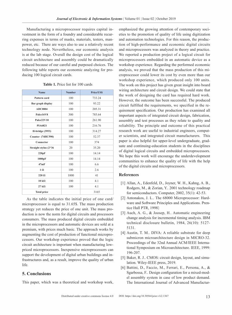
Manufacturing a microprocessor requires capital in-vestment in the form of a foundry and considerable recur-ring expenses in terms of masks, materials, testers, man-power, etc. There are ways also to use a relatively recent technology node. Nevertheless, our economic analysis is at the lab stage. Overall the design cost of the logical circuit architecture and assembly could be dramatically reduced because of our careful and purposed choices. The following table reports our economic analyzing for pro-ducing 100 logical circuit cards.

Table 1. Price list for 100 cards

Name Number Price/US$

Pattern card 100 733.24

Bar graph display 100 93.22

ADC0804 100 205.31

Palce16V8 300 785.64

Palce22V10 100 261.90

PIA6821 100 216.76

H-bridge (3953) 100 314.27

Counter (74HC590) 100 52.37

Connector 100 374

Straight stylus (2*36 20 35.20

220pF 100 14.14

1000pF 100 14.14

47mF 100 6.6

1 Ω 100 2.6

220 Ω 1000 41

10 kΩ 100 4.1

27 kΩ 100 4.1

Total price 3165

As the table indicates the initial price of one card/microprocessor is equal to 31.65$. The mass production strategy yet reduces the price of one unit. The mass pro-duction is now the norm for digital circuits and processors consumers. The mass produced digital circuits embedded in the microprocessors and automatic devices are sold at a premium, with prices much basic. The approach works by augmenting the cost of production of functional micropro-cessors. Our workshop experience proved that the logic circuit architecture is important when manufacturing low-priced microprocessors. Inexpensive microprocessors can support the development of digital urban buildings and in-frastructures and, as a result, improve the quality of urban life.

5. Conclusions

This paper, which was a theoretical and workshop work,

emphasized the growing attention of contemporary soci-eties to the promotion of quality of life using digitization and automation technologies. For this reason, the produc-tion of high-performance and economic digital circuits and microprocessors was analyzed in theory and practice. We reported a production project of a logical circuit for microprocessors embedded in an automatic device as a workshop experience. Regarding the performed economic analysis, we proved that the mass production of this mi-croprocessor could lower its cost by even more than our workshop experience, which produced only 100 units. The work on this project has given great insight into board wiring architecture and circuit design. We could state that the work of designing the card has required hard work. However, the outcome has been successful. The produced circuit fulfilled the requirements, we specified in the re-quirement specification. Our production has examined all important aspects of integrated circuit design, fabrication, assembly and test processes as they relate to quality and reliability. The principle and outcome of this practical research work are useful to industrial engineers, comput-er scientists, and integrated circuit manufacturers. This paper is also helpful for upper-level undergraduate, grad-uate and continuing-education students in the disciplines of digital logical circuits and embedded microprocessors. We hope this work will encourage the underdevelopment communities to enhance the quality of life with the help of the digital circuits and microprocessors.

References

[1] Allan, A., Edenfeld, D., Joyner, W. H., Kahng, A. B., Rodgers, M., & Zorian, Y.. 2001 technology roadmap for semiconductors. Computer, 2002, 35(1): 42-53.

[2] Antonakos, J. L.. The 68000 Microprocessor: Hard-ware and Software Principles and Applications. Pren-tice Hall PTR, 1998.‏

[3] Auch, A. G., & Joosep, H.. Automatic engineering change analysis for incremental timing analysis. IBM technical disclosure bulletin, 1984, 26(10): 5127-5131.

[4] Austin, T. M.. DIVA: A reliable substrate for deep submicron microarchitecture design in MICRO-32. Proceedings of the 32nd Annual ACM/IEEE Interna-tional Symposium on Microarchitecture. IEEE, 1999: 196-207.

[5] Baker, R. J.. CMOS: circuit design, layout, and simu-lation. Wiley-IEEE press, 2019.

[6] Battini, D., Faccio, M., Ferrari, E., Persona, A., & Sgarbossa, F.. Design configuration for a mixed-mod-el assembly system in case of low product demand. The International Journal of Advanced Manufactur-


14



ing Technology, 2007, 34(1-2): 188-200.[7] Bischof, C. H., Roh, L., & Mauer‐Oats, A. J..

ADIC: an extensible automatic differentiation tool for ANSI‐C. Software: Practice and Experience, 1997, 27(12): 1427-1456.

[8] Boothroyd, G.. Assembly automation and product design. CRC Press, 2005.

[9] Card, S. K.. The psychology of human-computer in-teraction. CRC Press, 2018.

[10] Ebrahimzadeh, I., Shahraki, A. A., Shahnaz, A. A., & Myandoab, A. M.. Progressing urban development and life quality simultaneously. City, Culture and So-ciety, 2016, 7(3): 186-193.

[11] Giordano, G.. Buying Power: As Industry 4.0 contin-ues to influence the plastics industry, manufacturers must consider connectivity and other factors when purchasing equipment. Plastics Engineering, 2019, 75(1): 28-35.

[12] Hemert, L. H.. Digitala kretsar. Studentlitteratur, ‏.2001

[13] Hnatek, E. R.. Integrated circuit quality and reliabili-ty. CRC Press, 1994.

[14] Koç, T. Ç.. The importance of high technology for economic development: a comparative analysis of Turkey and South Korea (Master’s thesis, Işık Üniversitesi), 2019.

[15] Libes, D.. Exploring Expect: a Tcl-based toolkit for automating interactive programs. O’Reilly Media, Inc., 1995.

[16] Maheshwary, S.. Automated Feature Construction and Selection (Doctoral dissertation, International In-stitute of Information Technology Hyderabad), 2019.

[17] Nichols, J., Myers, B. A., & Litwack, K.. Improving automatic interface generation with smart templates. In Proceedings of the 9th international conference on Intelligent user interfaces. ACM, 2004: 286-288.

[18] Patterson, D. A., & Sequin, C. H.. Design consider-ations for single-chip computers of the future. IEEE Journal of Solid-State Circuits, 1980, 15(1): 44-52.

[19] Paul, B. K., Panat, R., Mastrangelo, C., Kim, D., & Johnson, D.. Manufacturing of smart goods: Current state, future potential, and research recommenda-tions. Journal of Micro and Nano-Manufacturing, 2016, 4(4): 044001.

[20] Peatman, J. B.. Microcomputer-based design. Mc-Graw-Hill, Inc., 1977.

[21] Shahraki, A. A.. Regional development assessment: Reflections of the problem-oriented urban planning. Sustainable cities and society, 2017, 35: 224-231.

[22] Shahraki, A. A.. Supplying water in hydro-drought regions with case studies in Zahedan. Sustainable Water Resources Management, 2019, 5(2): 655-665.

[23] Siddiquee, N. A.. E-government and transformation of service delivery in developing countries: The Ban-gladesh experience and lessons. Transforming Gov-ernment: People, Process and Policy, 2016, 10(3): 368-390.

[24] Sugihara, T., Yamamoto, K., & Nakamura, Y.. Hard-ware design of high performance miniature anthropo-morphic robots. Robotics and Autonomous Systems, 2008, 56(1): 82-94.

[25] Tersine, R. J.. Production/Operations Management: Concepts. Structure and Analysis, 1985, 2.‏

[26] Turkoglu, H.. Sustainable development and quality of urban life. Procedia-Social and Behavioral Scienc-es, 2015, 202: 10-14.

[27] Wright, I. C.. A review of research into engineering change management: implications for product design. Design Studies, 1997, 18(1): 33-42.

[28] Xu, L. D., Xu, E. L., & Li, L.. Industry 4.0: state of the art and future trends. International Journal of Pro-duction Research, 2018, 56(8): 2941-2962.‏


15





ARTICLE

The Experimental WSN Network for Underground Monitoring H2 Abundance in the Mine Atmosphere Karnasurt Mine Lovozero Lay-ered Alkaline Intrusion

Asavin A. M.1*　Puha V.V.2　Baskakov S.S.3　Chesalova E.I.4　Litvinov A.V.5 1. V.I. Vernadsky Institute of Geochemistry and Analytical Chemistry RAS, Moscow2. Geological Institute Kola Scientific Centre RAS, Apatity 3. Moscow State Technical University, Moscow 4. State Geological Museum RAS, Moscow 5. National Research Nuclear University “MEPFI”, Moscow


Article historyReceived: 16 January 2020 Accepted: 6 March 2020Published Online: 31 March 2020

We have developed specialized equipment based on hydrogen mini-MDM sensors and the WSN telecommunication technology for long-term mon-itoring of hydrogen content in the environment. Unlike existing methods, the developed equipment makes it possible to carry out measurements directly in the explosion zone with high discreteness in time. This equip-ment was tested at a large rare-earth deposit of the Lovozero alkaline pluton Karnasurt in the underground mining tunnel. We observed a short time impulse very high concentration of hydrogen in the atmosphere (more than 3 orders of normal atmosphere concentration). This discovery is very important because at the time of the explosion one can create abnormally high concentrations of explosive mixtures of hydrocarbon gases that can leaded to accidents. The high resolving power of the our measurement equipment makes it possible in the first time in practical to determine the shape of the anomaly hydrogen of such a concentration and to calculate the volumes of hydrogen released from the rocks, at first time in the prac-tice. The shape of the anomaly usually consists of 2-3 additional peaks of the shape - “dragon-head” like. We make an first attempt is made to ex-plain this form of anomaly in the article. The aim of the work the estimate hydrogen emission in mining ore deposit of rare earth elements.

Keywords:HydrogenGas monitoringWSNMining depositEnvironment ecology

　

*Corresponding Author:Asavin A. M.,V.I. Vernadsky Institute of Geochemistry and Analytical Chemistry RAS, Moscow;Email: [email protected]

1. Introduction

Hydrogen is one of the most interesting trace gases found in the alkaline rocks. The emission of free hydrogen from ultrabasic rocks, associated with

serpentine forming processes, is the most well-known process. However, more recently attention was paid to

high hydrogen content in alkaline rocks [4]. The high con-centration of hydrocarbon and hydrogen-hydrocarbon gases in alkaline complexes link with occluded as fluid inclusions in minerals. These fact presences in the alka-line rock of hydrocarbon gases has a number of practical implications and it is therefore important to understand their source and distribution. Under certain conditions,

16



combustible and exposable gas components can accumu-late in the space of the underground mines. This may be a serious danger for the mining workflows and for human life and health. If you had to forecast an increase of gas emission in the mines, it is necessary to determine their spatial and time variations and a condition of their ap-pearance. According to their mobility, gas components are very sensitive to conditions of geological environment and can be effective indicators of the dangerous and adverse geodynamic factors.

Unfortunately, hydrogen is one of the most volatile gases, and therefore, when estimating of gas emission is made by traditional methods, there is the possibility that we measure only fragment of s some residual flux. We developed a specialized equipment based on MDM (semiconductors type) hydrogen sensors [3] and used WSN (wireless sensor network) telecommunication technology for long-time monitoring of hydrogen content in the atmosphere. Unlike existing methods, the developed equipment allows to carry out measurements directly in the zone of blasting operations with high discreteness in time.

2. Methods

The basic task of work is organization of the ecological monitoring in the district of exploitation of large deposits of apatite and rare earth elements ore deposit on the base of modern WSN technologies, consisting of sensors of gas H2, CH4, CO2, temperature, pressure, humidity by com-plex autonomous controls of telecommunications sensors network (used ZigBee protocol) (Figure 1).

Wireless sensor network monitoring (WSN) is last innovation for the industry. WSN are spatially distributed autonomous sensors to monitor physical or environmental conditions, such as gas, temperature, pressure, etc. and to cooperatively pass their data through the network to a main server location [2]. The WSN is built of “nodes” - from a few to several hundreds or even thousands, where each node is connected to one (or sometimes several) sensors. Each network node has a radio transceiver with an internal antenna or connection to an external antenna, a microcontroller, an electronic circuit for interfacing with the sensors and an energy source, usually a battery or an embedded form of energy harvesting. The project includes the development of informational and analytical system, which includes a network of gas emission sensors and internet webpage based on modern WEB-GIS technologies. The advantages of this technology is auton-omous work (to several months and more), programmable measurement of gas sensor, low cost (on one node of net-work), and possibility to connect to one node of supervi-sion a several types of sensors.

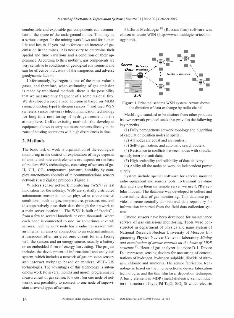
Platform MeshLogic [8] (Russian firm) software was chosen to create WSN (http://www.meshlogic.ru/technol-ogy.html).

Figure 1. Principal schema WSN system. Arrow shows the direction of data exchange by radio-chanel

MeshLogic standard to be distinct from other products its own network protocol stack that provides the following key benefits [1]:

(1) Fully homogenous network topology and algorithm of calculation position nodes in spatial;

(2) All nodes are equal and are routers;(3) Self-organization, and automatic search routers;(4) Resistance to conflicts between nodes with simulta-

neously inter transmit data;(5) High scalability and reliability of data delivery;(6) Ability all the nodes to work on independent power

supply.System include special software for service monitor

radio equipment and sensors tools. To transmit real-time data and store them on remote server we use GPRS cel-lular modem. The database was developed to collect and store online data of gas monitoring. This database pro-vides a secure centrally administered data repository for information imported from the field data collection sys-tem.

Unique sensors have been developed for maintenance service of gas emissions monitoring. Tools were con-structed in department of physics and nano system of National Research Nuclear University of Moscow En-gineering Physics Nuclear Center in laboratory Mining and examination of sensor controls on the basis of MDP structure [3]. Heart of gas analyzer is device D-1. Device D-1 represents sensing devices for measuring of concen-trations of hydrogen, hydrogen sulphide, dioxide of nitro-gen, chlorine and ammonia. The sensor fabrication tech-nology is based on the microelectronic device fabrication technologies and the thin film laser deposition technique. A basic element is MDP (metal-dielectric-semiconduc-tor) - structure of type Pd-Ta2O5-SiO2-Si which electric


17



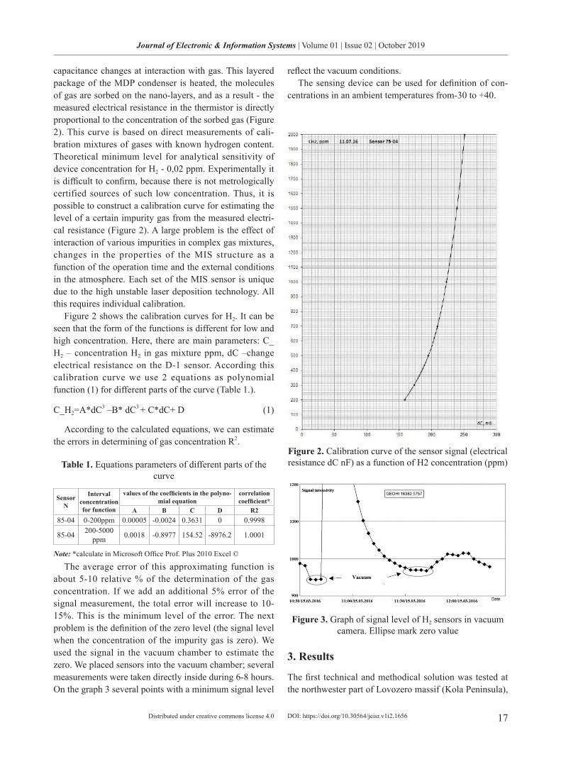
capacitance changes at interaction with gas. This layered package of the MDP condenser is heated, the molecules of gas are sorbed on the nano-layers, and as a result - the measured electrical resistance in the thermistor is directly proportional to the concentration of the sorbed gas (Figure 2). This curve is based on direct measurements of cali-bration mixtures of gases with known hydrogen content. Theoretical minimum level for analytical sensitivity of device concentration for H2 - 0,02 ppm. Experimentally it is difficult to confirm, because there is not metrologically certified sources of such low concentration. Thus, it is possible to construct a calibration curve for estimating the level of a certain impurity gas from the measured electri-cal resistance (Figure 2). A large problem is the effect of interaction of various impurities in complex gas mixtures, changes in the properties of the MIS structure as a function of the operation time and the external conditions in the atmosphere. Each set of the MIS sensor is unique due to the high unstable laser deposition technology. All this requires individual calibration.

Figure 2 shows the calibration curves for H2. It can be seen that the form of the functions is different for low and high concentration. Here, there are main parameters: C_H2 – concentration H2 in gas mixture ppm, dC –change electrical resistance on the D-1 sensor. According this calibration curve we use 2 equations as polynomial function (1) for different parts of the curve (Table 1.).

C_H2=A*dC3 –B* dC3 + C*dC+ D (1)

According to the calculated equations, we can estimate the errors in determining of gas concentration R2.

Table 1. Equations parameters of different parts of the curve

Sensor N

Interval concentration for function

values of the coefficients in the polyno-mial equation

correlation coefficient*

A B C D R285-04 0-200ppm 0.00005 -0.0024 0.3631 0 0.9998

85-04 200-5000 ppm 0.0018 -0.8977 154.52 -8976.2 1.0001

Note: *calculate in Microsoft Office Prof. Plus 2010 Excel ©

The average error of this approximating function is about 5-10 relative % of the determination of the gas concentration. If we add an additional 5% error of the signal measurement, the total error will increase to 10-15%. This is the minimum level of the error. The next problem is the definition of the zero level (the signal level when the concentration of the impurity gas is zero). We used the signal in the vacuum chamber to estimate the zero. We placed sensors into the vacuum chamber; several measurements were taken directly inside during 6-8 hours. On the graph 3 several points with a minimum signal level

reflect the vacuum conditions. The sensing device can be used for definition of con-

centrations in an ambient temperatures from-30 to +40.

Figure 2. Calibration curve of the sensor signal (electrical resistance dC nF) as a function of H2 concentration (ppm)

Figure 3. Graph of signal level of H2 sensors in vacuum camera. Ellipse mark zero value

3. Results

The first technical and methodical solution was tested at the northwester part of Lovozero massif (Kola Peninsula),


18



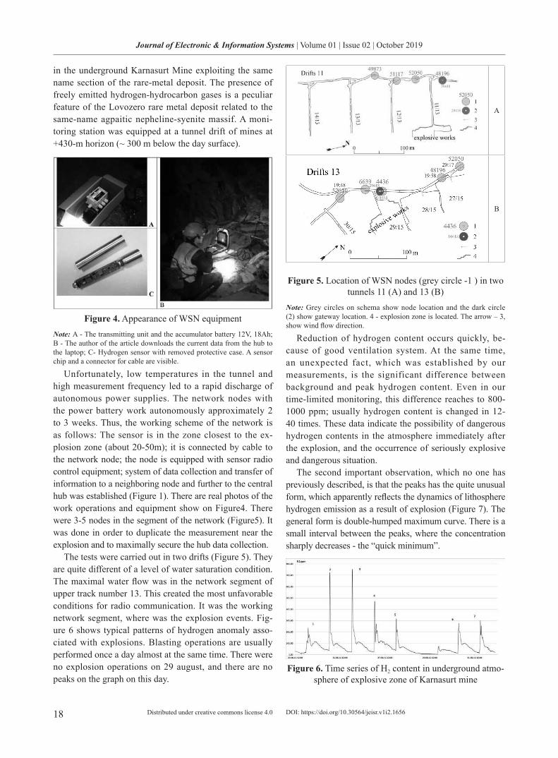
in the underground Karnasurt Mine exploiting the same name section of the rare-metal deposit. The presence of freely emitted hydrogen-hydrocarbon gases is a peculiar feature of the Lovozero rare metal deposit related to the same-name agpaitic nepheline-syenite massif. A moni-toring station was equipped at a tunnel drift of mines at +430-m horizon (~ 300 m below the day surface).

Figure 4. Appearance of WSN equipmentNote: A - The transmitting unit and the accumulator battery 12V, 18Ah; B - The author of the article downloads the current data from the hub to the laptop; C- Hydrogen sensor with removed protective case. A sensor chip and a connector for cable are visible.

Unfortunately, low temperatures in the tunnel and high measurement frequency led to a rapid discharge of autonomous power supplies. The network nodes with the power battery work autonomously approximately 2 to 3 weeks. Thus, the working scheme of the network is as follows: The sensor is in the zone closest to the ex-plosion zone (about 20-50m); it is connected by cable to the network node; the node is equipped with sensor radio control equipment; system of data collection and transfer of information to a neighboring node and further to the central hub was established (Figure 1). There are real photos of the work operations and equipment show on Figure4. There were 3-5 nodes in the segment of the network (Figure5). It was done in order to duplicate the measurement near the explosion and to maximally secure the hub data collection.

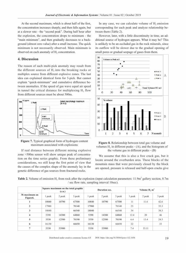
The tests were carried out in two drifts (Figure 5). They are quite different of a level of water saturation condition. The maximal water flow was in the network segment of upper track number 13. This created the most unfavorable conditions for radio communication. It was the working network segment, where was the explosion events. Fig-ure 6 shows typical patterns of hydrogen anomaly asso-ciated with explosions. Blasting operations are usually performed once a day almost at the same time. There were no explosion operations on 29 august, and there are no peaks on the graph on this day.

А

B

Figure 5. Location of WSN nodes (grey circle -1 ) in two tunnels 11 (A) and 13 (B)

Note: Grey circles on schema show node location and the dark circle (2) show gateway location. 4 - explosion zone is located. The arrow – 3, show wind flow direction.

Reduction of hydrogen content occurs quickly, be-cause of good ventilation system. At the same time, an unexpected fact, which was established by our measurements, is the significant difference between background and peak hydrogen content. Even in our time-limited monitoring, this difference reaches to 800-1000 ppm; usually hydrogen content is changed in 12-40 times. These data indicate the possibility of dangerous hydrogen contents in the atmosphere immediately after the explosion, and the occurrence of seriously explosive and dangerous situation.

The second important observation, which no one has previously described, is that the peaks has the quite unusual form, which apparently reflects the dynamics of lithosphere hydrogen emission as a result of explosion (Figure 7). The general form is double-humped maximum curve. There is a small interval between the peaks, where the concentration sharply decreases - the “quick minimum”.

Figure 6. Time series of H2 content in underground atmo-sphere of explosive zone of Karnasurt mine


19



At the second maximum, which is about half of the first, the concentration increases sharply, and then falls again, but at a slower rate - the “second peak”. During half hour after the explosion, the concentration drops to minimum - the “main minimum”, and then gradually decreases to a back-ground (almost zero value) after a small increase. The quick minimum is not necessarily observed. Main minimum is observed on each anomaly of H2 concentration.

4. Discussion

The reason of such multi-pick anomaly may result from the different sources of H2 into the breaking rocks or multiplex source from different explosive zones. The last idea can explained identical form for 3-pick. But cannot explain “quick-minimum” and cumulative difference be-tween anomalies. If the speed of gas wave equal air speed in tunnel the critical distance for multiplexing H2 flow from different sources must be about 500m.

Figure 7. Typical graphical form of hydrogen content maximum associated with explosions

If real distance between different mining explosive zone >500m sensor will show unique peak of concentra-tion on the time series graphic. From these preliminary considerations, we still keep the first point of view that the causes of the complex shape of the anomaly lay in the genetic difference of gas sources from fractured rocks.

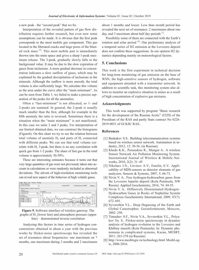
In any case, we can calculate volume of H2 emission corresponding for each peak and analyze relationship be-tween them (Table 2).

However, later, with a little discontinuity in time, an ad-ditional source of hydrogen appears. What it may be? This is unlikely to be an occluded gas in the rock minerals, since its outflow will be slower due to the gradual opening of small pores or gradual seepage of gases from them.

A

B

Figure 8. Relationship between total gas volume and volumes H2 in different peaks - (A), and the histogram of

the volume gas in different peaks - (B)

We assume that this is also a free crack gas, but it locate around the overburden area. These blocks of the mountain mass that were previously closed by the block are opened, pressure is released and half-open cracks give

Table 2. Volume of emission H2 from rock after the explosion (input calculation parameters: 11.9m2 gallery section, 0.7m / sec flow rate, sampling interval 10sec).

Square maximum on the total graphic (c.u.) Duration sec. Volume H2 m

3

maximum on Figure6. 1 peak 2 peak 3 peak 1 peak 2 peak 3 peak 1 peak 2 peak 3 peak

1 10840 10790 67500 10840 10790 67500 11 11.6 42.6

2 17980 70140 17980 70140 23 35.3

3 18040 66540 18040 66540 34 38.3

4 5390 14380 64860 5390 14380 64860 12.4 20 46

5 3530 12580 70190 3530 12580 70190 6.4 13.4 24.5

6 16130 66650 16130 66650 22 33

7 5330 53980 5330 53980 7.4 33.11


20



a new peak - the “second peak” that we fix. Interpretation of the revealed pattern of gas flow dis-

tribution requires further research, but even now some assumptions can be made. It is obvious that the first peak corresponds to the most mobile gas component. This gas located in the liberated cracks and large pores of the blast-ed rock mass [5]. This most mobile part is immediately thrown into the mine space and gives a sharp 1-peak max-imum release. The 3-peak, gradually slowly falls to the background value. It may be due to the slow expiration of gases from inclusions. A more gradual decrease in concen-tration indicates a slow outflow of gases, which may be explained by the gradual decrepitation of inclusions in the minerals. Although the outflow is more smooth, the total volume is also sufficiently large. We calculate this volume as the area under the curve after the “main minimum”. As can be seen from Table 1, we failed to make a precise sep-aration of the peaks for all the anomalies.

Often a “fast-minimum” is not allocated, so 1- and 2-peaks are summed. In general, the 2-peak is usually much smaller than the first, although for example in the fifth anomaly the ratio is reversed. Sometimes there is a situation when the “main minimum” is not manifested. In this case we unite 2 and 3 peaks. For interpretation of our limited obtained data, we can construct the histograms (Figure6). On this chart we try to see the relation between total volume of anomaly H2 and parts of H2 connected with different peaks. We can see that total volume cor-relate with H2 3-peak, but there is no any correlation with quick gas from 1-2 peaks. The share of fast gas in the total volume is approximately 30-50%.

These are interesting estimates because it turns out that very large quantities of gas were not previously taken into ac-count in calculations or were randomly included as abnormal deviations. The advent of high-resolution monitoring tools can reveal new aspect of the behavior of high volatile gases.

Figure 9. Software interface of wireless gateway. The graphs of H2 (lower line) and atmosphere pressure (upper

line) – demonstrated inverse correlation

Analyzing this factors in time series of hydrogen con-centrations obtained in about a year with the previous works by flicker-noise spectroscopy has revealed the set of resonance about frequencies: one maximum on 7 months, one maximum during 2 months and 2 maximums

about 1 months and lesser. Less than month period has revealed the next set of resonance: 2 maximums about one day, and 3 maximum about half day periods [7].

Possibility some of them are connected with the Earth’s rotation and solar period [6]. Our preliminary analysis of a temporal series of H2 emission at the Lovozero deposit does not confirm these suggestions. In our opinion H2 dy-namics depending mainly on meteorological factors.

5. Conclusions

This work is the first experiment in technical decision for long-term monitoring of gas emission on the base of WSN, the high-sensitive sensors of hydrogen, software and equipment attended with a transmitter network. In addition to scientific task, this monitoring system also al-lows to monitor an explosive situation in mines as a result of high concentration of explosive gas mixtures.

Acknowledgments

This work was supported by program “Basic research for the development of the Russian Arctic” (I32П) of the Presidium of the RAS and partly State contract No 0226-2019-0051 of GI KSC RAS..

References

[1] Baskakov S.S.. Building telecommunication systems based on wireless sensor network. Automation in in-dustry, 2012, 12: 30-36. (in Russian).

[2] Khedo K.K., Perseedoss R., Mungur A.. A wireless Sensor Network Air Pollution Monitoring System. International Journal of Wireless & Mobile Net-works, 2010, 2(2): 31–45

[3] Nikolaev I.N., Litvinov A.V., Emelin, E.V.. Appli-cability of MDS-sensors as detector elements of gas analyzers. Sensors & Systems, 2007, 5: 66-73.

[4] Nivin V. A.. Free hydrogen-hydrocarbon gases from the Lovozero loparite deposit (Kola Peninsula, NW Russia). Applied Geochemistry, 2016, 74: 44-55.

[5] Nivin V. A.. Diffusively Disseminated Hydrogen–Hydrocarbon Gases in Rocks of Nepheline Syenite Complexes Geochemistry International, 2009, 47(7): 672–691.

[6] Syvorotkin V.L.. Deep Degassing of the Earth and Global Catastrophes. Geoinformtsentr, Moscow, 2002: 250.

[7] Timashev S.F., Nivin V.A., Syvorotkin V.L., Polya-kov Yu. S.. Flicker-noise spectroscopy in dynamic analysis of hydrogen evolution in the Lovozero and Khibiny massifs (Kola Peninsula). In: Dynamic phe-nomena in complicated systems, Kazan, MESRT, 2011: 263-278 (in Russian).

[8] http://www.meshlogic.ru/technology.html MeshLog-ic, 2006-2016.


21





ARTICLE

Three Median Relations of Target Azimuth in one Dimensional Equi-distant Double Array

Tao Yu* China electronics technology corporation, China


Article historyReceived: 25 March 2020 Accepted: 9 April 2020Published Online: 31 May 2020

On the basis of the linear positioning solution of one-dimensional equi-distant double-base linear array, by proper approximate treatment of the strict solution, and by using the direction finding solution of single base path difference, the sinusoidal median relation of azimuth angle at three stations of the linear array is obtained. By using the sinusoidal median relation, the arithmetic mean solution of azimuth angle at three stations is obtained. All these results reveal the intrinsic correlation between the azimuth angles of one-dimensional linear array.

Keywords:AzimuthDouble-base arraySingle base direction findingArithmetic meanMedian relationshipPassive location

　

*Corresponding Author:Tao Yu,China electronics technology corporation, China;Email: [email protected]

1. Introduction

If based on strict mathematical derivation, there will be a tangent median relationship between the three sites of one-dimensional equal-spaced line array [1]. Strict-

ly speaking, the tangent median relation may not be the original result given in the literature [1], because the author seems to have seen the same or similar results in a paper, but the provenance was not immediately available.

In this paper, based on the linear positioning solution of one-dimensional equidistant double-base linear array [1], the sinusoidal median relationship of azimuth angle at three stations of the array is given by proper approximate processing of the strict linear solution and by using the di-rection finding solution of single-base path difference. By

using the sinusoidal median relation, the arithmetic mean solution of azimuth angle at three stations is obtained. For the convenience of reading and correction of the original errors, the derivation process of linear positioning solution of one-dimensional equidistant double base array and the derivation process of tangent median relation are given in this paper.

The results of this paper show that there are not only strict tangent median relation, but also approximate si-nusoidal median relation and approximate azimuth angle median relation. Up to now, most of the researches on pas-sive positioning systems only arrange mathematical equa-tions from the perspective of solving unknown quantities, but do not study the internal correlation among various parameters in depth. In fact, one-dimensional linear arrays

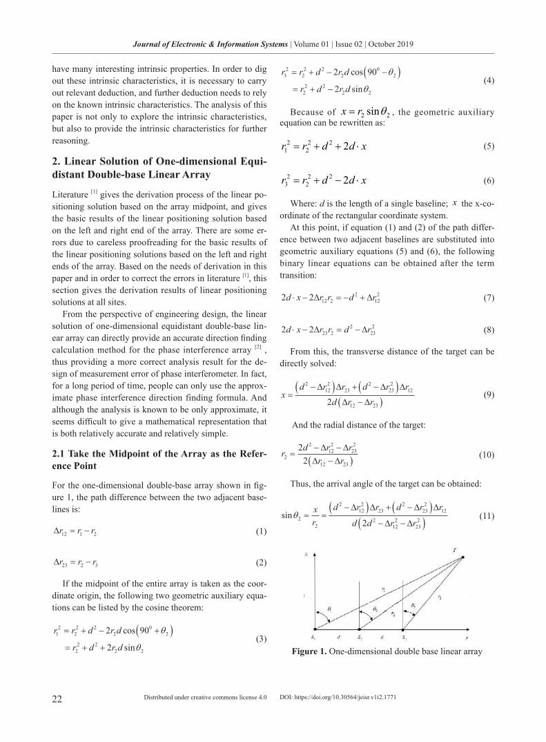
22



have many interesting intrinsic properties. In order to dig out these intrinsic characteristics, it is necessary to carry out relevant deduction, and further deduction needs to rely on the known intrinsic characteristics. The analysis of this paper is not only to explore the intrinsic characteristics, but also to provide the intrinsic characteristics for further reasoning.

2. Linear Solution of One-dimensional Equi-distant Double-base Linear Array

Literature [1] gives the derivation process of the linear po-sitioning solution based on the array midpoint, and gives the basic results of the linear positioning solution based on the left and right end of the array. There are some er-rors due to careless proofreading for the basic results of the linear positioning solutions based on the left and right ends of the array. Based on the needs of derivation in this paper and in order to correct the errors in literature [1], this section gives the derivation results of linear positioning solutions at all sites.

From the perspective of engineering design, the linear solution of one-dimensional equidistant double-base lin-ear array can directly provide an accurate direction finding calculation method for the phase interference array [2] , thus providing a more correct analysis result for the de-sign of measurement error of phase interferometer. In fact, for a long period of time, people can only use the approx-imate phase interference direction finding formula. And although the analysis is known to be only approximate, it seems difficult to give a mathematical representation that is both relatively accurate and relatively simple.

2.1 Take the Midpoint of the Array as the Refer-ence Point

For the one-dimensional double-base array shown in fig-ure 1, the path difference between the two adjacent base-lines is:

∆ = −r r r12 1 2 (1)

∆ = −r r r23 2 3 (2)

If the midpoint of the entire array is taken as the coor-dinate origin, the following two geometric auxiliary equa-tions can be listed by the cosine theorem:

r r d r d1 2 2 22 2 2 0= + − +

= + +r d r d2 2 22 2

2 cos 90

2 sinθ

( θ ) (3)

r r d r d3 2 2 22 2 2 0= + − −

= + −r d r d2 2 22 2

2 cos 90

2 sinθ

( θ ) (4)

Because of 22 sinθrx = , the geometric auxiliary equation can be rewritten as:

xddrr ⋅++= 2222

21 (5)

xddrr ⋅−+= 2222

23 (6)

Where: d is the length of a single baseline; x the x-co-ordinate of the rectangular coordinate system.

At this point, if equation (1) and (2) of the path differ-ence between two adjacent baselines are substituted into geometric auxiliary equations (5) and (6), the following binary linear equations can be obtained after the term transition:

2 2d x r r d r⋅ − ∆ = − + ∆12 2 122 2 (7)

2 2d x r r d r⋅ − ∆ = − ∆23 2 232 2 (8)

From this, the transverse distance of the target can be directly solved:

x =(d r r d r r2 2 2 2− ∆ ∆ + − ∆ ∆12 23 23 12

2d r r)(∆ − ∆12 23

()

) (9)

And the radial distance of the target:

r2 =2d r r

2(2 2 2

∆ −∆−∆ −∆r r12 23

12 23

) (10)

Thus, the arrival angle of the target can be obtained:

sinθ2 = =rx

2

(d r r d r r2 2 2 2− ∆ ∆ + − ∆ ∆

d d r r(12 23 23 12

2)

2 2 2− ∆ −∆

(12 23 )

) (11)

Figure 1. One-dimensional double base linear array


23



2.2 Take the Left End of the Array as the Refer-ence

Since the distance and orientation between the target and the leftmost site of the detection array are solved, the positioning equation is established by taking the leftmost position of the array as the coordinate origin. At this time, the geometric auxiliary equation listed by the cosine theo-rem is:

r r d r d2 1 1 12 2 2= + − −2 cos 90( θ ) (12)

r r d r d3 1 1 12 2 2= + − −4 4 cos 90( θ ) (13)

The path difference equation adopted should be:

∆ = −r r r12 1 2 (14)

∆ = −r r r13 1 3 (15)

The above two equations are substituted into equations (12) and (13) respectively, and the following binary linear equations are obtained after the term transfer:

2 2d x r r d r⋅ − ∆ = − ∆12 1 122 2 (16)

4 2 4d x r r d r⋅ − ∆ = − ∆13 1 132 2 (17)

From this, we can directly solve:

x =(4d r r d r r2 2 2 2− ∆ ∆ − − ∆ ∆

2 213 12 12 13

d r r)( ∆ − ∆12 13

()

) (18)

r1 =2 2d r r

2 2(2 2 2+ ∆ −∆∆ −∆r r12 13

12 13

) (19)

From the target position parameter obtained, the target arrival angle at the left end of the array can be obtained:

sinθ1 =(4d r r d r r2 2 2 2− ∆ ∆ − − ∆ ∆

d d r r(2 213 12 12 13)

2 2 2+ ∆ −∆

(12 13 )

) (20)

2.3 Take the Right End of the Array as the Refer-ence

To solve the distance and azimuth between the target and the site at the rightmost end of the detection array, the positioning equation is established by taking the position at the rightmost end of the array as the coordinate origin.

At this time, the geometric auxiliary equation listed by the cosine theorem is:

r r d r d1 3 3 32 2 2= + − +4 4 cos 90( θ ) (21)

r r d r d2 3 3 32 2 2= + − +2 cos 90( θ ) (22)

The path difference equation adopted should be:

∆ = −r r r23 2 3 (23)

∆ = −r r r13 1 3 (24)

By substituting the above two equations into the geo-metric auxiliary equations (21) and (22), the following binary linear equations can be obtained after the term transfer:

4 2 4d x r r r d⋅ − ∆ = ∆ −13 3 132 2 (25)

2 2d x r r r d⋅ − ∆ = ∆ −23 3 232 2 (26)

From this, we can directly solve:

x =(4d r r d r r2 2 2 2− ∆ ∆ − − ∆ ∆

2 213 23 23 13

d r r)(∆ − ∆13 23

()

) (27)

r3 =2 2d r r

2 2(2 2 2

∆ − ∆+ ∆ −∆r r13 23

23 13

) (28)

sinθ3 =(4d r r d r r2 2 2 2− ∆ ∆ − − ∆ ∆

d d r r(2 213 23 23 13)

2 2 2+ ∆ −∆

(23 13 )

) (29)

3. Three Median Relationships

3.1 The Direction Finding Solution of Single base Path Difference Obtained by Approximate Sim-plification

For the direction-finding equation (11) derived by taking the midpoint of the whole array as the coordinate origin, if the higher-order terms of the path difference contained in the equation are simplified to be approximately equal ∆ ≈ ∆r r12 23

2 2 , then:

sinθ ≈ =(d r r r2 2

2

− ∆ ∆ + ∆

d d r(2 1 2

2 2

)(− ∆ 1 )

) (∆ + ∆r r1 2

2d)

(30)


24



Due to:

∆ = − = − + − = ∆ + ∆r r r r r r r r r13 1 3 1 2 2 3 1 2( ) ( ) (31)

Therefore, there is a single-base direction finding solu-tion:

sinθ =∆2rd13 (32)

It is verified by simulation that the reference datum of single base path difference direction finding is at the midpoint of the whole baseline length. As far as the ex-pression form of the obtained single-base direction find-ing formula is concerned, the analysis result given by the author seems to be only a shift correction to the measure-ment datum of the existing approximate direction finding formula. And it is through this simple shift that the single - base direction finding formula is obtained.

The practical engineering significance of this result is that it provides a method for direction finding with long baseline time difference [3]. Theoretically, the exact solu-tion can be obtained based on multi-station time differ-ence measurement, but in the actual engineering design process, multi-station is often difficult to be located on a straight line. In this way, it is necessary to consider the di-rection finding problem of non-straight line, and the mea-surement error of angle between baselines will be gener-ated. According to the existing analysis [4], the included angle error has a relatively large impact on the positioning accuracy. Therefore, two-station high precision direction finding is more worthy of consideration.

3.2 Tangent Median Relationship

For the one-dimensional equidistant double-base array shown in figure 1, the radial distance of the three stations is projected onto the x axis and y axis respectively, and the following identities can be obtained:

2 2 1 1sin sinr r dθ θ= − (33)

2 2 3 3sin sinr r dθ θ= + (34)

2 2 1 1cos cosr rθ θ= (35)

2 2 3 3cos cosr rθ θ= (36)

If equations (33) and (34) are added, we can get:

2 2 1 1 3 32 sin sin sinr r rθ θ θ= + (37)

Then, substitute equation (35) and equation (36) into the above equation to eliminate the radial distance r1 and r3, and get:

2 3 22 1 22 2

1 3

sin cossin cos2 sin

cos cosrrr

θ θθ θθ

θ θ= + (38)

From this, it can be concluded that there exists the following tangent median relationship among the arrival angles of three sites:

2 1 32tg tg tgθ θ θ= + (39)

3.3 Sum of Sine Angles at the Two Endpoints of the Double Array

Add the direction-finding equations (20) and (29) at the left and right endpoints of the array:

sin sinθ θ1 3+ =

+(

(

4

4

d r r d r r

d r r d r r

2 2 2 2

2 2 2 2

− ∆ ∆ − − ∆ ∆

−∆ ∆ − −∆ ∆

d d r r

d d r r

(

(

2 2

2 2

13 23 23 13

13 12 12 13

)

)

2 2 2

2 2 2

+ ∆ −∆

+ ∆ −∆

(23 13

(12 13

)

))

)

(40)

Make approximate processing for the path difference of single base array:

∆ ≈ ∆r r12 130.5 (41)

∆ ≈ ∆r r23 130.5 (42)

After sorting, on the right side of the equation (40):

The right side of the equation 2≈∆2rd13 (43)

Therefore, the formula (32) in the previous section is quoted as follows:

sin sin 2sinθ θ θ1 3 2+ ≈ (44)

That is to say, the sinusoidal angles of the three sites approximately meet the arithmetic mean, and the obtained sinusoidal median relation is very similar to the tangent median relation.

3.4 Sum of Azimuth Angles at Two Endpoints of the Double Array

Use the trig formula, the sum of two sinusoidal angles of formula (20) and formula (29) can be converted into:


25



sin sin 2sin cosθ θ1 3+ =

θ θ θ θ1 3 1 3+ −2 2

(45)

Using equation (37), there is an approximate relation-ship:

sin cos sin

θ θ θ1 3 13+ ∆2 2

≈ θ2 (46)

For remote direction finding, since the intersec-tion angle Δθ13 is small, it can be approximated that cos(0.5Δθ13)≈1, so there are:

θ θ1 3+2

≈θ2 (47)

That is, the arithmetic mean of azimuth at the two end-points is approximately equal to the azimuth of the mid-point of the baseline. Previous studies by the author have shown that, the deviation characteristics of the approxi-mate direction-finding errors of two adjacent single-base arrays are exactly opposite [5]. If the arithmetic average of the approximate direction-finding results of two adjacent single-base arrays in one dimension is taken, the arithme-tic average of the two direction-finding values can be used to get the result that the deviation of the direction-finding error is close to zero by using an offsetting method.

4. Conclusion

The tangent mean relation is derived strictly, while the sine mean relation and the arithmetic mean of azimuth are approximate results. The results of this paper can be understood from two different perspectives: On the one hand, it seems that there are many magical features about

one-dimensional linear array. The azimuth at three stations not only satisfies the tangent median relation, but also ap-proximately satisfies the sinusoidal median relation, and also approximately satisfies the azimuth angle median re-lation. In fact, in reference [1], the author also studies that there exists the properties of arithmetic series between adjacent processes.

On the other hand, it is actually strictly proved that the arithmetic mean of azimuth of two endpoints is not equal to the angle value of the intermediate site. In fact, existing research and analysis show that, in most analytical anal-ysis, the positioning solution of one-dimensional array has a high requirement for the accuracy of calculation of direction-finding angle, and a few differences will make it difficult to get correct results. Therefore, the results of this paper undoubtedly have guiding significance for the subsequent analysis.

References

[1] Tao Yu . Technology of Passive detection loca-tion[M]. National defense industry press, 2017

[2] Tao Yu. Accurate Solution of DF Formula for Phase Interference with One-Dimensional Double Base-line[J]. Journal of Antennas, 2012,1(01): 8-11.

[3] Tao Yu. An Ultra-precision Time Difference DF Al-gorithm Based on Long Baseline[J]. Radio Engineer-ing, 2015, 45(9): 34-36.

[4] Jianhua Shao. Short baseline time difference di-rection finding technology and its application prospect[J]. Aerospace Electronic Warfare, 1997(4): 23-25.

[5] Tao Yu. Arithmetical Average Method of DF for Phase Interference One-Dimensional Double Base-line[J]. Modern Navigation, 2013, 4(5): 371-374.


Author GuidelinesThis document provides some guidelines to authors for submission in order to work towards a seamless submission

process. While complete adherence to the following guidelines is not enforced, authors should note that following

through with the guidelines will be helpful in expediting the copyediting and proofreading processes, and allow for

improved readability during the review process.

Ⅰ. Format

Program: Microsoft Word (preferred)

Font: Times New Roman

Size: 12

Style: Normal

Paragraph: Justified

Required Documents

Ⅱ. Cover Letter

All articles should include a cover letter as a separate document.

The cover letter should include:

Names and affiliation of author(s)

The corresponding author should be identified.

Eg. Department, University, Province/City/State, Postal Code, Country

A brief description of the novelty and importance of the findings detailed in the paper

Declaration

v Conflict of Interest

Examples of conflicts of interest include (but are not limited to):

Research grants

Honoria

Employment or consultation

Project sponsors

Author’s position on advisory boards or board of directors/management relationships

Multiple affiliation

Other financial relationships/support

Informed Consent

This section confirms that written consent was obtained from all participants prior to the study.

Ethical Approval

Eg. The paper received the ethical approval of XXX Ethics Committee.

Trial Registration

Eg. Name of Trial Registry: Trial Registration Number

Contributorship

The role(s) that each author undertook should be reflected in this section. This section affirms that each credited author

has had a significant contribution to the article.

1. Main Manuscript

2. Reference List

3. Supplementary Data/Information

Supplementary figures, small tables, text etc.

As supplementary data/information is not copyedited/proofread, kindly ensure that the section is free from errors, and is

presented clearly.

Ⅲ. Abstract

A general introduction to the research topic of the paper should be provided, along with a brief summary of its main

results and implications. Kindly ensure the abstract is self-contained and remains readable to a wider audience. The

abstract should also be kept to a maximum of 200 words.

Authors should also include 5-8 keywords after the abstract, separated by a semi-colon, avoiding the words already used

in the title of the article.

Abstract and keywords should be reflected as font size 14.

Ⅳ. Title

The title should not exceed 50 words. Authors are encouraged to keep their titles succinct and relevant.

Titles should be reflected as font size 26, and in bold type.

Ⅳ. Section Headings

Section headings, sub-headings, and sub-subheadings should be differentiated by font size.

Section Headings: Font size 22, bold type

Sub-Headings: Font size 16, bold type

Sub-Subheadings: Font size 14, bold type

Main Manuscript Outline

Ⅴ. Introduction

The introduction should highlight the significance of the research conducted, in particular, in relation to current state of

research in the field. A clear research objective should be conveyed within a single sentence.

Ⅵ. Methodology/Methods

In this section, the methods used to obtain the results in the paper should be clearly elucidated. This allows readers to be

able to replicate the study in the future. Authors should ensure that any references made to other research or experiments

should be clearly cited.

Ⅶ. Results

In this section, the results of experiments conducted should be detailed. The results should not be discussed at length in

this section. Alternatively, Results and Discussion can also be combined to a single section.

Ⅷ. Discussion

In this section, the results of the experiments conducted can be discussed in detail. Authors should discuss the direct and

indirect implications of their findings, and also discuss if the results obtain reflect the current state of research in the field.

Applications for the research should be discussed in this section. Suggestions for future research can also be discussed in

this section.

Ⅸ. Conclusion

This section offers closure for the paper. An effective conclusion will need to sum up the principal findings of the papers,

and its implications for further research.

Ⅹ. References

References should be included as a separate page from the main manuscript. For parts of the manuscript that have

referenced a particular source, a superscript (ie. [x]) should be included next to the referenced text.

[x] refers to the allocated number of the source under the Reference List (eg. [1], [2], [3])

In the References section, the corresponding source should be referenced as:

[x] Author(s). Article Title [Publication Type]. Journal Name, Vol. No., Issue No.: Page numbers. (DOI number)

Ⅺ. Glossary of Publication Type

J = Journal/Magazine

M = Monograph/Book

C = (Article) Collection

D = Dissertation/Thesis

P = Patent

S = Standards

N = Newspapers

R = Reports

Kindly note that the order of appearance of the referenced source should follow its order of appearance in the main manu-

script.

Graphs, Figures, Tables, and Equations

Graphs, figures and tables should be labelled closely below it and aligned to the center. Each data presentation type

should be labelled as Graph, Figure, or Table, and its sequence should be in running order, separate from each other.

Equations should be aligned to the left, and numbered with in running order with its number in parenthesis (aligned

right).

Ⅻ. Others

Conflicts of interest, acknowledgements, and publication ethics should also be declared in the final version of the manu-

script. Instructions have been provided as its counterpart under Cover Letter.

Bilingual Publishing Co. (BPC) is an international publisher of online, open access and scholarly peer-reviewed journals covering a wide range of academic disciplines including science, technology, medicine, engineering, education and social science. Reflecting the latest research from a broad sweep of subjects, our content is accessible world-wide——both in print and online.

BPC aims to provide an analytics as well as platform for information exchange and discussion that help organizations and professionals in advancing society for the betterment of mankind. BPC hopes to be indexed by well-known databases in order to expand its reach to the science community, and eventually grow to be a reputable publisher recognized by scholars and researchers around the world.

BPC adopts the Open Journal Systems, see on ojs.bilpublishing.com

Database Inclusion

China National KnowledgeInfrastructure

Asia & Pacific ScienceCitation Index Creative Commons

Google Scholar Crossref MyScienceWork

About the Publisher