Embed Size (px)
Citation preview
arX
iv:0
912.
4247
v1 [
nlin
.PS]
21
Dec
200
9
Drift And Meander Of Spiral Waves
Thesis submitted in accordance with the requirements ofthe University of Liverpool for the degree of Doctor in Philosophy
by
Andrew J. Foulkes
March 2009
Abstract
In this thesis, we are concerned with the dynamics of spiral wave solutions to
Reaction-Diffsion systems of equations, and how they behave when subject to sym-
metry breaking perturbations.
We present an asymptotic theory of the study of meandering (quasiperiodic spiral
wave solutions) spiral waves which are drifting due to symmetry breaking perturbations.
This theory is based on earlier theories: the 1995 Biktashev et al theory of drift of
rigidly rotating spirals [14], and the 1996 Biktashev et al theory of meander of spirals
in unperturbed systems [16]. We combine the two theories by first rewriting the 1995
drift theory using the symmetry quotient system method of the 1996 meander theory,
and then go on to extend the approach to meandering spirals by considering Floquet
theory and using a singular perturbation method. We demonstrate the work of the
newly developed theory on simple examples.
We also develop a numerical implementation of the quotient system method, demon-
strate its numerical convergence and its use in calculations which would be difficult to
do by the standard methods, and also link this study to the problem of calculation of
response functions of spiral waves.
i
Declaration
No part of the work referred to in this Thesis have been submitted in support of
an application for another degree or qualification of this or any other institution of
learning. However, some parts of the material contained herein have been previously
published.
ii
Contents
Abstract i
Declaration ii
Contents v
List of Figures ix
Acknowledgements x
1 Introduction 1
2 Literature Review 3
2.1 Spiral Waves . . . . . . . . . . . . . . . . . . . . . . . . . . . . . . . . . 3
2.2 Spiral Wave Dynamics . . . . . . . . . . . . . . . . . . . . . . . . . . . . 8
2.3 Models used in Numerical Analysis . . . . . . . . . . . . . . . . . . . . . 31
2.4 Numerical Methods & Software . . . . . . . . . . . . . . . . . . . . . . . 34
3 Asymptotic Theory of Drift and Meander 40
3.1 Introduction . . . . . . . . . . . . . . . . . . . . . . . . . . . . . . . . . . 40
3.2 Drift of a Rigidly Rotating Spiral Wave . . . . . . . . . . . . . . . . . . 41
3.3 Drift of a Rigidly Rotating Spiral Wave: Examples . . . . . . . . . . . . 60
3.4 Floquet Theory - Periodic Solutions . . . . . . . . . . . . . . . . . . . . 76
3.5 Application to the Quotient System . . . . . . . . . . . . . . . . . . . . 98
3.6 Drift & Meander Example: Resonant Drift . . . . . . . . . . . . . . . . 101
3.7 Frequency Locking . . . . . . . . . . . . . . . . . . . . . . . . . . . . . . 106
3.8 Conclusion & Further Work . . . . . . . . . . . . . . . . . . . . . . . . . 113
4 Initial Numerical Analysis 115
4.1 Introduction . . . . . . . . . . . . . . . . . . . . . . . . . . . . . . . . . . 115
4.2 Inhomogeneity Induced Drift of Spiral Wave . . . . . . . . . . . . . . . . 115
4.3 Electrophoretic Induced Drift of Spiral Wave . . . . . . . . . . . . . . . 123
iii
4.4 Generic Forms for the Equation of motion . . . . . . . . . . . . . . . . . 128
4.5 Conclusion . . . . . . . . . . . . . . . . . . . . . . . . . . . . . . . . . . 132
5 Numerical Solutions of Spiral Waves in a Moving Frame of Reference134
5.1 Introduction . . . . . . . . . . . . . . . . . . . . . . . . . . . . . . . . . . 134
5.2 Numerical Implementation . . . . . . . . . . . . . . . . . . . . . . . . . . 135
5.3 Examples: Rigidly Rotation and Meander . . . . . . . . . . . . . . . . . 148
5.4 Convergence Testing of EZ-Freeze . . . . . . . . . . . . . . . . . . . . . . 159
5.5 Application I: 1:1 Resonance in Meandering Spiral Waves . . . . . . . . 178
5.6 Application II: Large Core Spirals . . . . . . . . . . . . . . . . . . . . . 186
5.7 Conculsion . . . . . . . . . . . . . . . . . . . . . . . . . . . . . . . . . . 196
6 Numerical Calculation of Response Functions 197
6.1 Introduction . . . . . . . . . . . . . . . . . . . . . . . . . . . . . . . . . . 197
6.2 Response Functions & Their Importance . . . . . . . . . . . . . . . . . . 198
6.3 Numerical Implementation . . . . . . . . . . . . . . . . . . . . . . . . . . 201
6.4 Generation of Initial Conditions . . . . . . . . . . . . . . . . . . . . . . . 204
6.5 Examples: ec.x . . . . . . . . . . . . . . . . . . . . . . . . . . . . . . . . 210
6.6 Convergence Testing . . . . . . . . . . . . . . . . . . . . . . . . . . . . . 212
6.7 Conculsion . . . . . . . . . . . . . . . . . . . . . . . . . . . . . . . . . . 219
7 Conclusions & Further Work 220
A Definitions 222
A.1 Dynamical System . . . . . . . . . . . . . . . . . . . . . . . . . . . . . . 222
A.2 Quasiperiodicity . . . . . . . . . . . . . . . . . . . . . . . . . . . . . . . 222
A.3 Torus . . . . . . . . . . . . . . . . . . . . . . . . . . . . . . . . . . . . . 223
A.4 Bifurcations . . . . . . . . . . . . . . . . . . . . . . . . . . . . . . . . . . 224
A.5 Codimension (Codim) . . . . . . . . . . . . . . . . . . . . . . . . . . . . 233
A.6 Excitability . . . . . . . . . . . . . . . . . . . . . . . . . . . . . . . . . . 233
A.7 Euclidean Symmetry . . . . . . . . . . . . . . . . . . . . . . . . . . . . . 233
A.8 A Bit of Group Theory . . . . . . . . . . . . . . . . . . . . . . . . . . . . 236
A.9 Manifolds . . . . . . . . . . . . . . . . . . . . . . . . . . . . . . . . . . . 242
A.10 Banach Spaces . . . . . . . . . . . . . . . . . . . . . . . . . . . . . . . . 244
B EZ-Freeze 246
B.1 Getting Started: A Quick Guide . . . . . . . . . . . . . . . . . . . . . . 246
B.2 How it works - The Users Manual . . . . . . . . . . . . . . . . . . . . . . 251
B.3 How it works - The Programmers Manual . . . . . . . . . . . . . . . . . 256
iv

B.4 Mathematical Background . . . . . . . . . . . . . . . . . . . . . . . . . . 260
Bibliography 268
v
List of Figures
2.1 A Spiral Wave . . . . . . . . . . . . . . . . . . . . . . . . . . . . . . . . 4
2.2 Evolution of a Spiral Wave from a broken wave . . . . . . . . . . . . . . 6
2.3 Spiral wave tip: definition 1 . . . . . . . . . . . . . . . . . . . . . . . . . 8
2.4 Spiral wave tip: definition 2 . . . . . . . . . . . . . . . . . . . . . . . . . 8
2.5 A Rigidly Rotating Spiral Wave . . . . . . . . . . . . . . . . . . . . . . . 9
2.6 Hopf bifurcation transition from rigid rotation to meander . . . . . . . . 10
2.7 A Meandering Spiral Wave with inward facing petals . . . . . . . . . . . 11
2.8 A Meandering Spiral Wave with outward facing petals . . . . . . . . . . 11
2.9 Barkley’s Flower garden . . . . . . . . . . . . . . . . . . . . . . . . . . . 12
2.10 Meandering spiral wave from ODE system . . . . . . . . . . . . . . . . . 14
2.11 A snap shot of a spiral wave. . . . . . . . . . . . . . . . . . . . . . . . . 15
2.12 Functional space representation of a spiral wave solution . . . . . . . . . 17
2.13 Spiral wave tip location . . . . . . . . . . . . . . . . . . . . . . . . . . . 18
2.14 Meandering spiral waves: numerical solution . . . . . . . . . . . . . . . . 22
2.15 Meandering spiral waves: analytical solution . . . . . . . . . . . . . . . . 23
2.16 Drifting rigidly rotating spiral wave . . . . . . . . . . . . . . . . . . . . . 24
2.17 Barkley’s model: Phase Portrait . . . . . . . . . . . . . . . . . . . . . . 32
2.18 FHN model: Phase Portrait . . . . . . . . . . . . . . . . . . . . . . . . . 32
2.19 Barkley’s model: Phase Portrait showing the “δ” line. . . . . . . . . . . 33
3.1 Quotient system reduction in the functional space . . . . . . . . . . . . 44
3.2 Resonant drift: comparison of the analytical solution to numerical solution 64
3.3 Electrophoretic drift: comparison of the analytical and numerical solutions 70
3.4 2:1 Arnol’d Tongue . . . . . . . . . . . . . . . . . . . . . . . . . . . . . . 111
3.5 Poincare mapping . . . . . . . . . . . . . . . . . . . . . . . . . . . . . . 113
4.1 Inhomogeneitiy induced drift: gradient=0.0008 . . . . . . . . . . . . . . 117
4.2 Inhomogeneitiy induced drift: gradient vs. speed . . . . . . . . . . . . . 118
4.3 Inhomogeneitiy induced drift of a meandering spiral wave . . . . . . . . 121
4.4 Inhomogeneitiy induced drift: Quotient solution . . . . . . . . . . . . . . 122
vi
4.5 Inhomogeneitiy induced drift: translational velocities . . . . . . . . . . . 122
4.6 Inhomogeneitiy induced drift: cross section of the translational velocities 123
4.7 Electrophoretis induced drift: time vs. ω . . . . . . . . . . . . . . . . . . 125
4.8 Electrophoretis induced drift: a vs. ω0:ωH . . . . . . . . . . . . . . . . . 126
4.9 Electrophoretis induced drift: Trajectory for a=0.5530 . . . . . . . . . . 127
4.10 Electrophoretis induced drift: Trajectory for a=0.5540 . . . . . . . . . . 127
4.11 Electrophoretis induced drift: a vs. ω0:ωH . . . . . . . . . . . . . . . . . 127
4.12 Meandering spiral wave: trajectories . . . . . . . . . . . . . . . . . . . . 129
4.13 Meandering spiral wave: x and y components . . . . . . . . . . . . . . . 129
4.14 Drifting and meandering spiral wave: trajectory . . . . . . . . . . . . . . 131
4.15 Drifting and meandering spiral wave: x and y components . . . . . . . . 132
5.1 Calculation of the translational and rotational shifts. . . . . . . . . . . . 138
5.2 Analogy behind the third pinning condition. . . . . . . . . . . . . . . . . 142
5.3 Non-uniqueness of the revised tip pinning condition. . . . . . . . . . . . 144
5.4 Rigid Rotation in Barkley’s model and in the laboratory frame of reference.150
5.5 Rigid rotation: Barkley’s model, First order, Method 1. . . . . . . . . . 152
5.6 Rigid rotation: Barkley’s model, Second order, Method 1. . . . . . . . . 152
5.7 Rigid rotation: Barkley’s model, First order, Method 2. . . . . . . . . . 153
5.8 Rigid rotation: Barkley’s model, Second order, Method 2. . . . . . . . . 153
5.9 Meander in the FHN model and in the laboratory frame of reference. . . 154
5.10 Meander: FHN model, first order, method 1 . . . . . . . . . . . . . . . . 157
5.11 Meander: FHN model, second order, method 1 . . . . . . . . . . . . . . 157
5.12 Meander: FHN model, first order, method 2 . . . . . . . . . . . . . . . . 158
5.13 Meander: FHN model, second order, method 2 . . . . . . . . . . . . . . 158
5.14 Rigid rotation: dependency on the second pinning point . . . . . . . . . 159
5.15 Meander: dependency on the second pinning point . . . . . . . . . . . . 160
5.16 Spacestep convergence: Neumann boundary condition . . . . . . . . . . 164
5.17 Spacestep convergence: Neumann boundary conditions, final solutions . 165
5.18 Spacestep convergence: Dirichlet boundary conditions . . . . . . . . . . 166
5.19 Spacestep convergence: Dirichlet boundary conditions, final solutions . . 167
5.20 Box size convergence: Neumann boundary conditions . . . . . . . . . . . 169
5.21 Box size convergence: Neumann boundary conditions, final solutions . . 170
5.22 Box size convergence: Dirichlet boundary conditions . . . . . . . . . . . 171
5.23 Box size convergence: Dirichlet boundary conditions, final solutions . . . 172
5.24 Timestep convergence: Neumann boundary conditions . . . . . . . . . . 174
5.25 Timestep convergence: Neumann boundary conditions, final solutions . 175
5.26 Timestep convergence: Dirichlet boundary conditions . . . . . . . . . . . 176
vii
5.27 Timestep convergence: Dirichlet boundary conditions, final solutions . . 177
5.28 Parametric Portrait for FHN model with γ=0.5 [63] . . . . . . . . . . . 180
5.29 1:1 resonance testing run 1: trajectories . . . . . . . . . . . . . . . . . . 182
5.30 1:1 resonance testing run 1: quotient solutions . . . . . . . . . . . . . . . 183
5.31 1:1 resonance testing run 2: trajectories . . . . . . . . . . . . . . . . . . 184
5.32 1:1 resonance testing run 2: quotient solutions . . . . . . . . . . . . . . . 185
5.33 1:1 resonance testing run 3: trajectories . . . . . . . . . . . . . . . . . . 187
5.34 1:1 resonance testing run 2: quotient solutions . . . . . . . . . . . . . . . 188
5.35 Large core: a versus ω . . . . . . . . . . . . . . . . . . . . . . . . . . . . 191
5.36 Large core: a versus ω split either side of critical point . . . . . . . . . . 191
5.37 Spiral wave solution at the critical point . . . . . . . . . . . . . . . . . . 192
5.38 Large core: solutions . . . . . . . . . . . . . . . . . . . . . . . . . . . . . 193
5.39 Spiral wave solution at the critical point . . . . . . . . . . . . . . . . . . 193
5.40 Large core: right of critical point . . . . . . . . . . . . . . . . . . . . . . 194
5.41 Large core: left of critical point . . . . . . . . . . . . . . . . . . . . . . . 195
6.1 Determining the radius of the trajectory and the center of rotation . . . 207
6.2 Determination of the inscribed circle. . . . . . . . . . . . . . . . . . . . . 207
6.3 Linear Interpolation. . . . . . . . . . . . . . . . . . . . . . . . . . . . . . 209
6.4 Numerical solution of the Goldstone modes . . . . . . . . . . . . . . . . 211
6.5 Numerical solution of the response functions . . . . . . . . . . . . . . . . 211
6.6 Disk Size Convergence . . . . . . . . . . . . . . . . . . . . . . . . . . . . 214
6.7 Angular Convergence . . . . . . . . . . . . . . . . . . . . . . . . . . . . . 216
6.8 Radial Convergence . . . . . . . . . . . . . . . . . . . . . . . . . . . . . 218
A.1 A typical 2-Torus. . . . . . . . . . . . . . . . . . . . . . . . . . . . . . . 223
A.2 A traveling wave displaying propagation. . . . . . . . . . . . . . . . . . . 234
A.3 Rotation of the original axis . . . . . . . . . . . . . . . . . . . . . . . . . 235
A.4 Translational shift of a wave train . . . . . . . . . . . . . . . . . . . . . 239
A.5 Manifold illustration 1 . . . . . . . . . . . . . . . . . . . . . . . . . . . . 243
A.6 Manifold illustration 2 . . . . . . . . . . . . . . . . . . . . . . . . . . . . 243
A.7 The graph of f(x, t) with t fixed. . . . . . . . . . . . . . . . . . . . . . . 244
A.8 Banch space: a function in the original space . . . . . . . . . . . . . . . 244
A.9 The graph of f(x, t) for various fixed values of time. . . . . . . . . . . . 245
A.10 Banch space: a function in the Banach space . . . . . . . . . . . . . . . 245
B.1 Rigidly rotating spiral wave . . . . . . . . . . . . . . . . . . . . . . . . . 248
B.2 Rigidly rotating spiral wave tip trajectory reconstruction . . . . . . . . . 249
B.3 A meandering spiral wave . . . . . . . . . . . . . . . . . . . . . . . . . . 249
viii
B.4 Meandering spiral tip trajectory reconstruction . . . . . . . . . . . . . . 250
ix
Acknowledgements
There are many people who have supported me throughout my studies to which I
am in debt.
Firstly, my supervisor Vadim Biktashev. Your support to me over the last three
years has been fantastic, and I believe that without your assistance, intellect and un-
derstanding I would not be where I am today. I am particularly grateful for introducing
me to the wonderful world of programming. I have discovered a talent, with your as-
sistance, that I previously had no knowledge of. Finally, I would like to say bowoespasibo za vse Vy sdelali dl men za prowlye tri goda. budu vsegda imet~dolg k Vam.Secondly, to the lecturers and postdocs from the University of Liverpool who have
helped me throughout my studies. To Irina Biktasheva for your support and very useful
constructive comments regarding my work and involving in your research project. To
Bakhty Vasiev for many hours of your time discussing various numerical procedures. To
Radostin Simitev for his help with general computer, programming and LATEX matters.
Ozgur Selsil for being a good friend over the last three years and giving the support I
need.
To Mike Nieves, thanks for putting up with me over the last three years, for the
hours of discussions we’ve had and for being a good friend. To Stuart and Ibrahim,
again many thanks for being such good friends and also for all the help you have given
me over the last three years.
To my family, I thank you for believing in me and giving me all the support I have
needed over the last three years. To my Mum especially, without you behind me I
would not be here today writing this thesis. Words can’t express just how much you
mean to me. To my best mate Ste Winslow, I thank you for always being there and we
will forever be best mates.
Finally, to my wife. You have had to put up with a lot of mixed emotions over
the last three years. We have two lovely children and it has not been easy for us all,
especially in the last year of my studies. I thank you from the bottom of my heart for
being such a supportive wife and the mother of my lovely boys, Charlie and Sam.
x
Dedicated to Charlie and Sammy-Jo, my whole world.
xi
Publications
Some of the work presented within this thesis has been shown in the following
publications and presentations:
Publications
1. I.V. Biktasheva, D. Barkley, V.N. Biktashev, A.J. Foulkes, G.V. Bordyugov, Com-
putation of the response functions of spiral waves in active media, Phy. Rev. E,
2009 (in review)
2. A.J. Foulkes, V.N. Biktashev, Spiral Wave Solutions in a Comoving Frame of
Reference, 2009 (in preparation)
Presentations
1. “Dynamics of Spiral Waves Under Symmetry Breaking Perturbations”, 2008 PhD
Symposium, Department of Mathematical Science, The University of Liverpool,
21 May 2008 (talk).
2. “Group Theortical Approaches to Drift of Rigidly Rotating Spiral Waves”,Group
Seminars, Mathematical Cardiology Group, Department of Mathematical Sci-
ence, The University of Liverpool, April 2008 - August 2008 (series of talks).
3. “Drift and Meander of Spiral Waves”, Seminar - Liverpool Mathematical Biology
Group, Department of Mathematical Science, The University of Liverpool, 10 &
24 April 2008 (talk).
4. “Drift and Meander of Spiral Waves”, British Applied Mathematics Colloquium
2008, The University of Manchester, 3 April 2008 (talk).
5. “Towards a Theory of the Drift of Meandering Spiral Waves”, 2007 PhD Sympo-
sium, Department of Mathematical Science, The University of Liverpool, 22 May
2007 (talk).
6. “Meandering and Drifting Spiral Waves due to Inhomogeneities”, British Applied
Mathematics Colloquium 2007, The University of Bristol, 18 April 2007 (talk).
7. “Drift of Meandering Spiral Waves due to Inhomogeneities”, Annual Research
Day 2007, The University of Liverpool, 14 March 2007 (poster - 1st prize,
Dept. of Mathematical Sciences).
xii
8. “Spiral Wave Meander”, Group Seminars, Mathematical Cardiology Group, De-
partment of Mathematical Science, The University of Liverpool, August 2006 -
January 2007 (series of talks).
9. “Meander of Spiral Waves”, 2006 PhD Symposium, Department of Mathematical
Science, The University of Liverpool, 23 May 2006 (talk).
xiii
Chapter 1
Introduction
Spirals occur throughout Nature. From Spiral Galaxies that are many millions of
light years in diameter, to snail shells that are maybe only a centimetre or two across.
One important occurance of spirals in Nature is the presence of spiral wave in cardiac
tissue, and in particular spiral waves have been largely linked to the onset of Cardiac
Arrythmias. Hence, the study of the onset of these spiral waves, and how they behave,
is an area of research that has attracted a lot of attention over the years.
We are concerned with the dynamics of spiral wave solutions to Reaction-Diffusion
systems of equations, and how they behave when subject to symmetry breaking pertur-
bations. We present an asymptotic theory of the study of meandering (quasiperiodic
spiral wave solutions) spiral waves which are drifting due to symmetry breaking per-
turbations, as well as a numerical method to solve the quotient system derived from
the theory.
We also drew some motivation for the numerical studies from the initial work into
frequency locked spiral waves. It was noted that the spiral wave solutions used in this
initial analysis were conducted in a box which needed to be of a size such that the
numerical simulations did not take a long time to generate. Therefore, the answer to
this is to study the spiral wave solution in a frame of reference which is moving with the
tip of the wave, thereby ensuring that the spiral wave never reaches the boundaries and
enabling us to conduct the simulations for as long as would like, but using a relatively
small box size.
The structure of the thesis is detailed below:
• Chapter 2: Here we shall give an introduction to spiral waves. We will introduce
the main concepts and definitions, before giving a review of the main separate
theories of meander and drift. We will also give a review of the software we shall
use and the numerical methods implemented into the software.
• Chapter 3: In this chapter, we shall show our asymptotic theory of the drift
1
of meandering spiral waves. This is split into three distinct parts. The first
part is concerned with the rewriting of the theory of drift of a rigidly rotating
spiral wave using group theory as well as perturbation and asymptotic methods.
The first part is concluded with three examples of drift: viz. resonant drift;
electropheresis induced drift; and inhomogeneity induced drift. The extension of
this theory to meandering spiral waves is then achieved using Floquet theory. We
will review Floquet theory before applying it to our problem. We note that in
applying Floquet theory to our problem, we discovered that we required a singular
perturbation method in order to achieve boundedness in the perturbed part of
the solution. This singular perturbation technique took the form of a correction
to the time variable. We then end the chapter with some analysis of frequency
locking and how we used the results from the singular perturbation method to
obtain the Arnol’d Standard Mapping.
• Chapter 4: We will then show some of the initial numerical analysis we under-
took in the early stages of this work. We investigated frequency locking using
both inhomogeneity and electropheresis induced drift within Barkley’s model.
The results generated within this chapter motivated the work for Chap.5, since
it was clear that we needed either a larger box size in which to study frequency
locking or to study the spiral waves in a frame of reference comoving with the tip
of the spiral wave.
• Chapter 5: We shall then look at the numerical calculations of spiral waves in
a frame of reference that is comoving with the tip of the spiral wave. We shall
describe the methods that we use in this work and introduce the program that
was generated from this work - EZ-Freeze. We shall then show the results of the
testing of the program, before showing some examples and applications.
• Chapter 6: This chapter is concerned with the numerical calculation of the re-
sponse functions for spiral waves. The response functions are the eigenfunctions
relating to the critical eigenvalues of the adjoint linearised Reaction-Diffusion sys-
tem of equation. The analytical calculation of these is not possible and therefore
they can only be studied numerically. A program called evcospi is used in this
work. We will also show how EZ-Freeze can be used in the generation of the
initial conditions for evcospi, and explain why using EZ-Freeze is more accurate
than using other methods.
• Chapter 7: Finally, will conclude this work and describe some of the future
directions for this work.
2
Chapter 2
Literature Review
In this chapter we review the main papers upon which we build our research. We
commence with an introduction to spiral waves, detailing the nature of the spiral wave,
its features and its most important properties. The author will also include his own
account of the various properties of spiral waves.
We will then move on to the dynamics of the spiral wave and the sort of motion
that it can exhibit. We will start from the most basic type of spiral wave motion, Rigid
Rotation, before moving on to a more complicated type of motion known as Meander.
We will then round off the section with a review of a motion known as Drift. All these
reviews will be supported by the author’s own numerical analysis wherever the author
feels it necessary to help the reader.
The models used throughout our numerical work will then be discussed and several
key properties of each model used will be scrutinised. We will also provide an analysis
of the types of numerical methods used to solve such model (which are PDE’s), and
review the types of software that will be used to conduct the numerical methods.
Finally, we will conclude this chapter.
2.1 Spiral Waves
Spiral waves can be mathematically studied as spatio-temporal solutions to Reaction-
Diffusion type systems of equations. That is not to say that all solutions, where they
exist, to Reaction-Diffusion systems are spiral waves. Also, they can appear in non-
Reaction-Diffusion type systems such as the Hodgkin-Huxley system of equations. They
are, of course, dependent not only on initial conditions but also on the parameters of
the Reaction-Diffusion model used (as we will show later on). So, the equations we will
be considering are Reaction-Diffusion type equations:
∂u
∂t= D∇2u + f(u), where u, f ∈ R
n;D ∈ Rn×n, r = (x, y) ∈ R
2 (2.1)
3
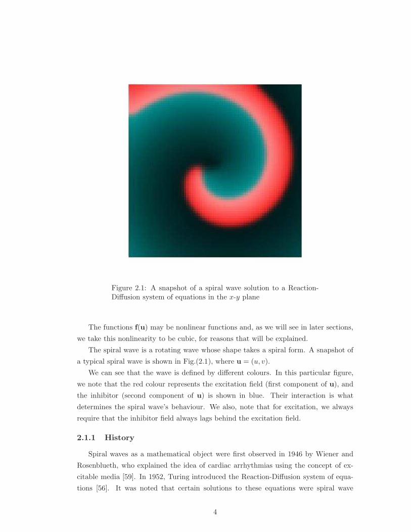
Figure 2.1: A snapshot of a spiral wave solution to a Reaction-Diffusion system of equations in the x-y plane
The functions f(u) may be nonlinear functions and, as we will see in later sections,
we take this nonlinearity to be cubic, for reasons that will be explained.
The spiral wave is a rotating wave whose shape takes a spiral form. A snapshot of
a typical spiral wave is shown in Fig.(2.1), where u = (u, v).
We can see that the wave is defined by different colours. In this particular figure,
we note that the red colour represents the excitation field (first component of u), and
the inhibitor (second component of u) is shown in blue. Their interaction is what
determines the spiral wave’s behaviour. We also, note that for excitation, we always
require that the inhibitor field always lags behind the excitation field.
2.1.1 History
Spiral waves as a mathematical object were first observed in 1946 by Wiener and
Rosenblueth, who explained the idea of cardiac arrhythmias using the concept of ex-
citable media [59]. In 1952, Turing introduced the Reaction-Diffusion system of equa-
tions [56]. It was noted that certain solutions to these equations were spiral wave
4
solutions. In the 1960’s, Belousov and Zhabotinski observed spiral patterns in light in-
tensive chemical reactions, now known as the Belousov-Zhabotinski Reaction, or simply
BZ-Reaction. It must be noted that they did not work together. Belousov initiated the
work [12], which was subsequently picked up by Zhabotinski several years later [66, 65].
However, their combined research is recognized in unison. This work was then made
popular in the West by Arthur Winfree in the early 1970’s, and it was to Winfree that
the discovery of meandering spiral waves (to be discuss in the next section) is credited
[61].
Since the 1970’s there has been a massive surge in the amount of research that has
taken place on spiral waves and their many physical occurrences - initiation of spiral
waves; transition from rigid rotation to meander; drift of spiral waves; frequency locking
within meandering waves and forced spiral waves, to name but a few.
We are primarily interested in the dynamics of meandering and drifting spiral waves.
As we progress through the following sections we will introduce the main concepts and
theories that we will be using, as well as several paper reviews that we feel are necessary.
In general, there are several excellent books on spiral waves and patterns formed
from Reaction-Diffusion systems. The first book is by Winfree and is a general intro-
duction to this area [62]. As Winfree states in his introduction, this book is primarily
about patterns that involve time - memory and heartbeat as just two examples. He then
splits the book into four parts. The first part is an introduction to arrhythmias, and
considers temporal patterns without any spatial organization. He looks at circadian
rhythms, as well as the heartbeat and other biological rhythms, and how these be-
have when interrupted. The second part considers spatially organised biological clocks,
particular the heartbeat, and how the presence of rotating waves can prove lethal to
the heartbeat. Then he extends the ideas introduced in the previous two parts to the
three dimensional case - scroll waves. In part four, he summarizes what he has intro-
duced and what questions remain outstanding. his book is extremely well written and
supported by many pictures and diagrams, a lot of which are coloured.
The next book is by Murray [48]. In fact this is a collection of two books in
Mathematical Biology gives an excellent introduction, at undergraduate level, to the
mathematics behind spiral waves. The main text that we are interested is found in
the second volume, Chapter 1, which describes various wave processes arising from
Reaction-Diffusion type equations. The section of this chapter that becomes most
interesting for our purposes is Section 1.6 et seq. Although the mathematical content
relating to spiral waves in this text is aimed at undergraduate level, it provides a general
background knowledge base for which to proceed into spiral wave research.
Another excellent publication is the book by Keener and Sneyd [37]. This covers a
vast array of areas relating to the physiology of the body. The sections of interest to us
5
y
x
y
x
y
x
y
x
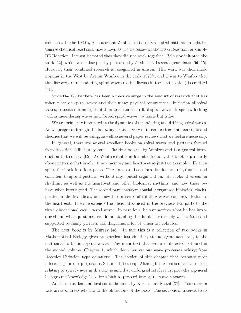
Figure 2.2: Evolution of a Spiral Wave from a broken wave [67].
appear in Chaps.9&10. Chap.9 introduces the mathematics behind a one dimensional
wave train, and introduces two classic models which simulate wave propagation, viz.
FitzHugh-Nagumo model and the Hodgkin-Huxley model. Also introduced is a singular
perturbation approach to studying these phenomena. Finally, Chap.10 briefly describes
the mathematics behind rotating waves (spiral waves) and how these waves can be
studied analytically, even though the models used are PDE’s which may not necessarily
have general analytical solutions.
The next book is a more advanced text by Zykov [67]. This, overall, is probably one
of the best books that has been produced which concentrates on solely waves in excitable
media. Zykov begins his book by describing the sort of systems that we may come across
which support the propagation of excitation waves. He also places high importance on
the use of computer modeling and simulation, and therefore taylors the text towards
such work. To sumarise the book briefly, Chap.1 introduces the concept of excitable
media and spiral waves. In particular, he introduces the sorts of equations that we are
likely to come across in this area of work, including the famed Belousov-Zhabotinski
Reaction. Chap.2 then gives a thorough review of the sorts of processes that we may
come across in biological excitable tissues. Chaps.3&4 present the methods to simulate
wave propagation in one and two dimensions, with particular reference to the initiation
of excitation waves. Chap.5 describes the simulation of waves in cardiac tissue, whilst in
Chap.6 Zykov presents a simplified approach to studying spiral wave processes in two-
dimensional excitable media in both bounded and unbounded dimensions. Chap.7 is
an investigation into the general properties of excitation circulation in two-dimensions,
and a simplified model is used in the simulations. Finally, Chap.8 deals with the issue
of controlling excitation waves and in particular, how to control excitation waves in
cardiac tissue. Overall, an excellent text for those wanting a thorough background
reading into this area.
6
2.1.2 Initiation
The subject of initiation of a spiral wave could be a Ph.D project in itself. Indeed,
several authors have studied this in great details [51, 1], and others have also looked at
the 1-D case (travelling waves) [34], but not so much the 3-D case (scroll waves). The
book by Zykov described in the previous section gives an excellent introduction into
the initial process of excitation waves. For our purposes, we are not concerned with
exactly how these wavesare initiated, but how theyevolve in time once they have been
initiated.
We will, however, give a brief description of how these wave are initiated. The
method which we will use, and which is implemented into the software we use, is
known as Cross Field Stimulation. This is when the spiral wave is initiated when two
plane waves, travelling perpendicular to each other, collide, form a broken wave and
evolveinto a spiral. Of course, not every collision resultin a spiral wave, but in our
simulation, the initial conditions are chosen such that a spiral wave is formed in most
instances.
So, once these waves have collided and a broken wave is formed, the spiral wave
then takes shape, as shown in Fig.(2.2), where the arrows in each picture show the
direction of motion of the excitation field. We also see that the inhibitor field is lagging
behind the excitation field as described above. So, we can see that it is this interaction
of the two fields that help form the wave.
2.1.3 Tip of the Spiral Wave
The location of the tip of the spiral is extremely important. Throughout our work,
we consider how the wave moves by studying the motion of the tip of the spiral wave.
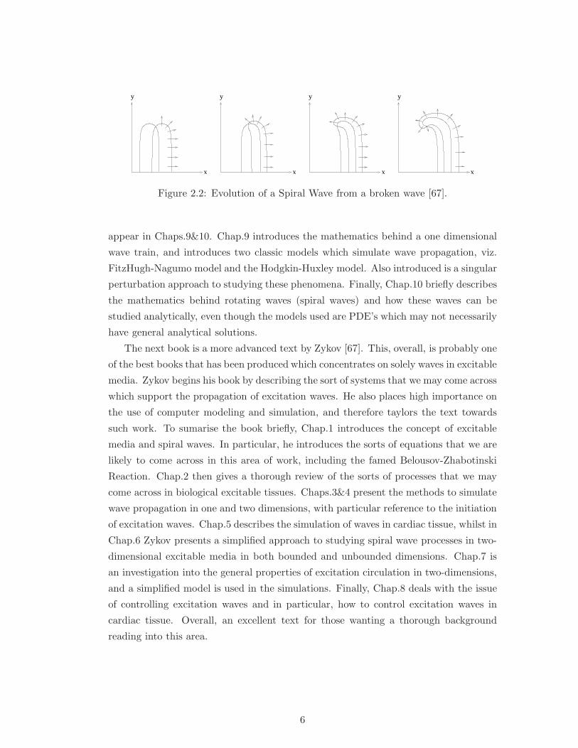
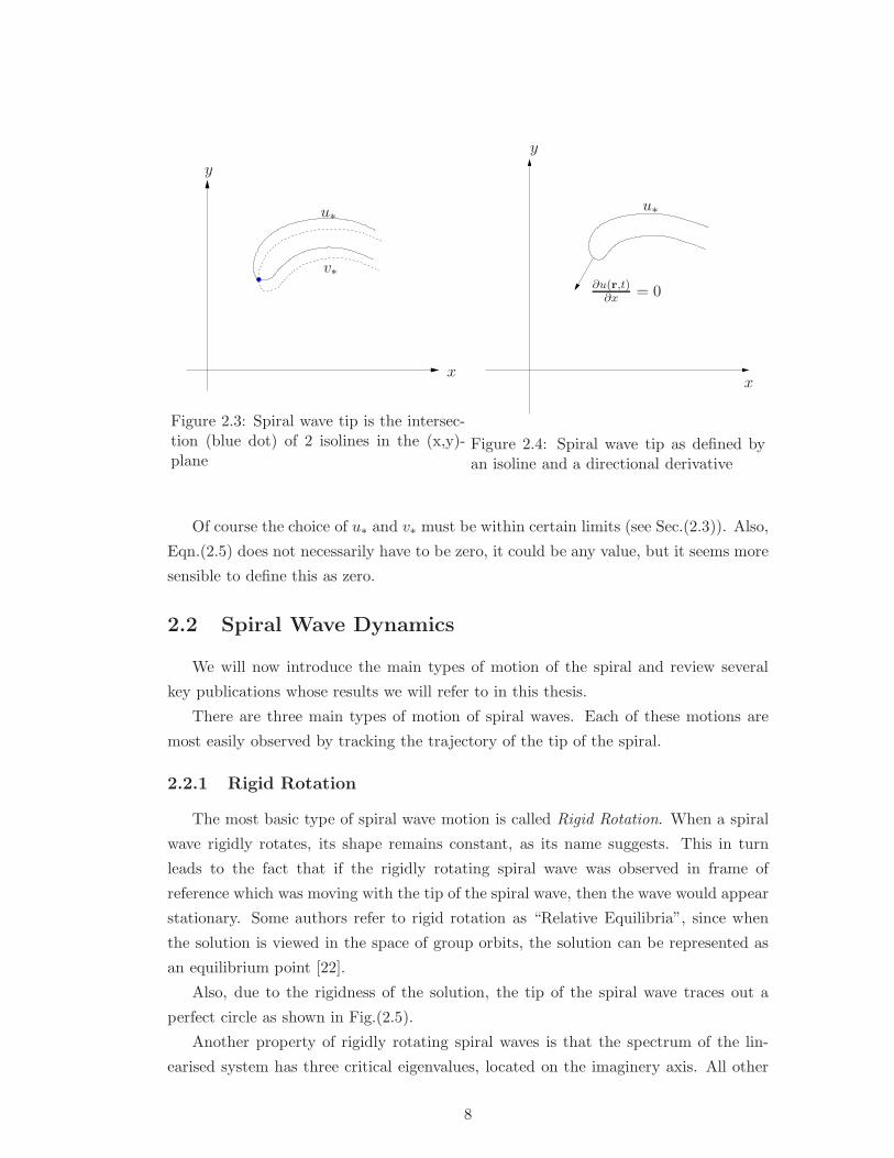
The most common way to define the tip of a spiral wave is to define two isolines -
one defined in the excitation field, and the other in the inhibitor field - and define the
tip as the intersection of the two lines, Fig.(2.3):
u(r, t) = u∗ (2.2)
v(r, t) = v∗ (2.3)
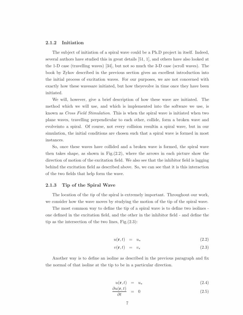
Another way is to define an isoline as described in the previous paragraph and fix
the normal of that isoline at the tip to be in a particular direction.
u(r, t) = u∗ (2.4)
∂u(r, t)
∂t= 0 (2.5)
7
y
x
u∗
v∗
Figure 2.3: Spiral wave tip is the intersec-tion (blue dot) of 2 isolines in the (x,y)-plane
∂u(r,t)∂x
= 0
x
y
u∗
Figure 2.4: Spiral wave tip as defined byan isoline and a directional derivative
Of course the choice of u∗ and v∗ must be within certain limits (see Sec.(2.3)). Also,
Eqn.(2.5) does not necessarily have to be zero, it could be any value, but it seems more
sensible to define this as zero.
2.2 Spiral Wave Dynamics
We will now introduce the main types of motion of the spiral and review several
key publications whose results we will refer to in this thesis.
There are three main types of motion of spiral waves. Each of these motions are
most easily observed by tracking the trajectory of the tip of the spiral.
2.2.1 Rigid Rotation
The most basic type of spiral wave motion is called Rigid Rotation. When a spiral
wave rigidly rotates, its shape remains constant, as its name suggests. This in turn
leads to the fact that if the rigidly rotating spiral wave was observed in frame of
reference which was moving with the tip of the spiral wave, then the wave would appear
stationary. Some authors refer to rigid rotation as “Relative Equilibria”, since when
the solution is viewed in the space of group orbits, the solution can be represented as
an equilibrium point [22].
Also, due to the rigidness of the solution, the tip of the spiral wave traces out a
perfect circle as shown in Fig.(2.5).
Another property of rigidly rotating spiral waves is that the spectrum of the lin-
earised system has three critical eigenvalues, located on the imaginery axis. All other
8
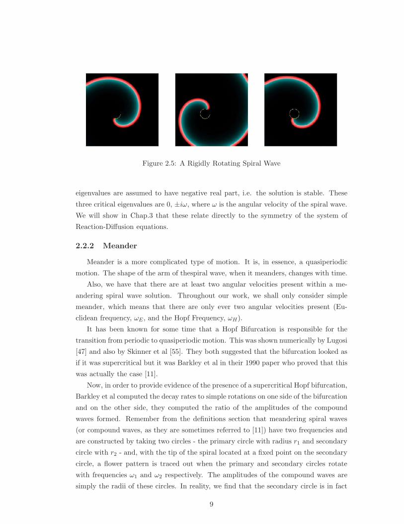
Figure 2.5: A Rigidly Rotating Spiral Wave
eigenvalues are assumed to have negative real part, i.e. the solution is stable. These
three critical eigenvalues are 0, ±iω, where ω is the angular velocity of the spiral wave.
We will show in Chap.3 that these relate directly to the symmetry of the system of
Reaction-Diffusion equations.
2.2.2 Meander
Meander is a more complicated type of motion. It is, in essence, a quasiperiodic
motion. The shape of the arm of thespiral wave, when it meanders, changes with time.
Also, we have that there are at least two angular velocities present within a me-
andering spiral wave solution. Throughout our work, we shall only consider simple
meander, which means that there are only ever two angular velocities present (Eu-
clidean frequency, ωE, and the Hopf Frequency, ωH).
It has been known for some time that a Hopf Bifurcation is responsible for the
transition from periodic to quasiperiodic motion. This was shown numerically by Lugosi
[47] and also by Skinner et al [55]. They both suggested that the bifurcation looked as
if it was supercritical but it was Barkley et al in their 1990 paper who proved that this
was actually the case [11].
Now, in order to provide evidence of the presence of a supercritical Hopf bifurcation,
Barkley et al computed the decay rates to simple rotations on one side of the bifurcation
and on the other side, they computed the ratio of the amplitudes of the compound
waves formed. Remember from the definitions section that meandering spiral waves
(or compound waves, as they are sometimes referred to [11]) have two frequencies and
are constructed by taking two circles - the primary circle with radius r1 and secondary
circle with r2 - and, with the tip of the spiral located at a fixed point on the secondary
circle, a flower pattern is traced out when the primary and secondary circles rotate
with frequencies ω1 and ω2 respectively. The amplitudes of the compound waves are
simply the radii of these circles. In reality, we find that the secondary circle is in fact
9
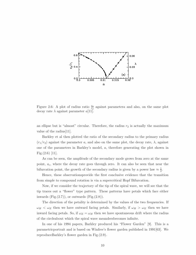
Figure 2.6: A plot of radius ratio r1r2
against parametera and also, on the same plotdecay rate λ against parameter a[11].
an ellipse but is “almost” circular. Therefore, the radius r2 is actually the maximum
value of the radius[11].
Barkley et al then plotted the ratio of the secondary radius to the primary radius
(r1/r2) against the parameter a, and also on the same plot, the decay rate, λ, against
one of the parameters in Barkley’s model, a, therefore generating the plot shown in
Fig.(2.6) [11].
As can be seen, the amplitude of the secondary mode grows from zero at the same
point, ac, where the decay rate goes through zero. It can also be seen that near the
bifurcation point, the growth of the secondary radius is given by a power law ≈ 12 .
Hence, these observationsprovide the first conclusive evidence that the transition
from simple to compound rotation is via a supercritical Hopf Bifurcation.
Now, if we consider the trajectory of the tip of the spiral wave, we will see that the
tip traces out a “flower” type pattern. These patterns have petals which face either
inwards (Fig.(2.7)), or outwards (Fig.(2.8)).
The direction of the petality is determined by the values of the two frequencies. If
ωH < ωE then we have outward facing petals. Similarly, if ωH > ωE then we have
inward facing petals. So, if ωE = ωH then we have spontaneous drift where the radius
of the circleabout which the spiral wave meandersbecomes infinite.
In one of his 1994 papers, Barkley produced his “Flower Garden” [9]. This is a
parametricportrait and is based on Winfree’s flower garden published in 1991[63]. We
reproduceBarkley’s flower garden in Fig.(2.9).
10
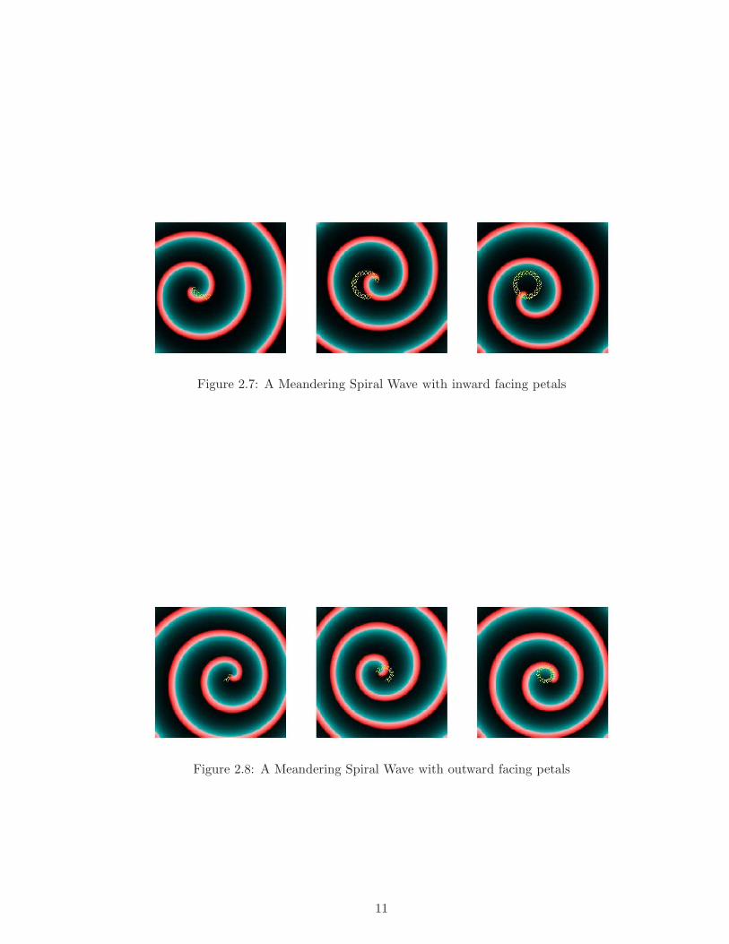
Figure 2.7: A Meandering Spiral Wave with inward facing petals
Figure 2.8: A Meandering Spiral Wave with outward facing petals
11
0
0.2
0.4
0.6
0.8
1
0 0.5 1 1.5 2
b
a
MRW
NW
NW
RW
RW
A
B D
C
E G F
MRW
NW
NW
RW
RW
A
B D
C
E G F
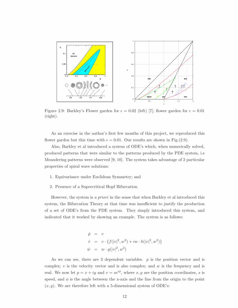
Figure 2.9: Barkley’s Flower garden for ǫ = 0.02 (left) [7]; flower garden for ǫ = 0.01(right).
As an exercise in the author’s first few months of this project, we reproduced this
flower garden but this time with ǫ = 0.01. Our results are shown in Fig.(2.9).
Also, Barkley et al introduced a system of ODE’s which, when numerically solved,
produced patterns that were similar to the patterns produced by the PDE system, i.e
Meandering patterns were observed [9, 10]. The system takes advantage of 2 particular
properties of spiral wave solutions:
1. Equivariance under Euclidean Symmetry; and
2. Presence of a Supercritical Hopf Bifurcation.
However, the system is a priori in the sense that when Barkley et al introduced this
system, the Bifurcation Theory at that time was insufficient to justify the production
of a set of ODE’s from the PDE system. They simply introduced this system, and
indicated that it worked by showing an example. The system is as follows:
p = v
v = v · f(|v|2, w2) + iw · h(|v|2, w2)w = w · g(|v|2, w2)
As we can see, there are 3 dependent variables. p is the position vector and is
complex; v is the velocity vector and is also complex; and w is the frequency and is
real. We now let p = x + iy and v = seiφ, where x, y are the position coordinates, s is
speed, and φ is the angle between the x-axis and the line from the origin to the point
(x, y). We are therefore left with a 5-dimensional system of ODE’s:
12
x = s cos(φ), y = s sin(φ)
φ = w · h(s2, w2), s = s · f(s2, w2), w = w · g(s2, w2)
As you can see, we have 3 unknown functions, f(s2, w2), g(s2, w2) and h(s2, w2),
and it is up to the reader to define exactly what these functions are. Barkley et al took
these functions and Taylor expanded them as follows:
f(s2, w2) = α0 + α1s2 + α2w
2 + α3s4
g(s2, w2) = β0 + β1s2 + β2w
2
h(s2, w2) = γ0
After assigning specific values to α0, α3, β0, β1 and β2, and letting ξ = s2 and
ζ = w2, we get the following reduced system:
ξ = 2ξf(ξ, ζ)
ζ = 2ζg(ξ, ζ)
where:
f(ξ, ζ) = −1
4+ α1ξ + α2ζ − ξ2
g(ξ, ζ) = ξ − ζ − 1
h(ξ, ζ) = γ0
We can now take this reduced system and use our usual dynamical system and
bifurcation analysis to shown that, for α1 = 103 , there is a Hopf Bifurcation at α2 = −5
and γ0 =√
28.
In order to verify that the patterns produced by the system of ODE’s are the same
as those produced by the PDE’s, we created a simple C program which numerically
solved the 5-dimensional system of ODE’s with the parameters α1, α2 and γ0 being the
parameters that are varied, with the other parameters being kept at the values specified
above. We observed that the patterns produced were the same as those produced by
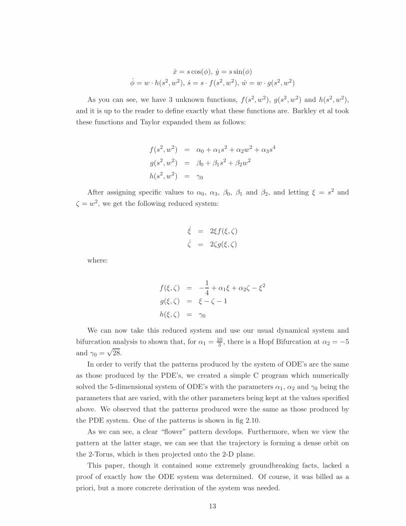
the PDE system. One of the patterns is shown in fig 2.10.
As we can see, a clear “flower” pattern develops. Furthermore, when we view the
pattern at the latter stage, we can see that the trajectory is forming a dense orbit on
the 2-Torus, which is then projected onto the 2-D plane.
This paper, though it contained some extremely groundbreaking facts, lacked a
proof of exactly how the ODE system was determined. Of course, it was billed as a
priori, but a more concrete derivation of the system was needed.
13
-0.4
-0.2
0
0.2
0.4
0.6
0.8
1
0.4 0.6 0.8 1 1.2 1.4 1.6 1.8-0.4
-0.2
0
0.2
0.4
0.6
0.8
1
0.4 0.6 0.8 1 1.2 1.4 1.6 1.8
Figure 2.10: Results from numerical analysis of the ODE system taken from the sametip file but at different time intervals
This was then motivation for Biktashev et al [16] to derive a system of equations
the describe the dynamics of the tip of a meandering spiral wave. We will review this
publication in more detail.
Theory of Meander [16]
Biktashev et al considered the special Euclidean group SE(2), together with the
following reaction diffusion equation:
∂tu = D∇2u + f(u) (2.6)
for u = u(r, t) = (u(1), u(2), . . . , u(l)) ∈ Rl, l ≥ 2, r = (x, y) ∈ R
2. As mentioned,
previously, this system is equivariant under transformations belonging to SE(2). A
proof of this is shown in the appendix (Sec.(A.8.9)). So, if u(r, t) is a solution then so
too is u(r, t) such that:
u(r, t) = T (g)u(r, t), ∀g ∈ SE(2) (2.7)
where T (g) is the group action of g ∈ SE(2) on the function u(r, t).
Let us for a moment think about the group SE(2). This group is concerned with
translations and rotations in the 2 dimensional plane, (x, y). Therefore, the elements
of SE(2) concerns only spatial transformations, not temporal transformations. Now, if
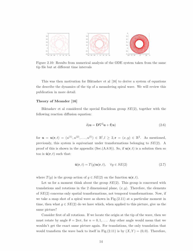
we take a snap shot of a spiral wave as shown in Fig.(2.11) at a particular moment in
time, then what g ∈ SE(2) do we have which, when applied to this picture, give us the
same picture?
Consider first of all rotations. If we locate the origin at the tip of the wave, then we
must rotate by angle θ = 2nπ, for n = 0, 1, . . .. Any other angle would mean that we
wouldn’t get the exact same picture again. For translations, the only translation that
would transform the wave back to itself in Fig.(2.11) is by (X,Y ) = (0, 0). Therefore,
14
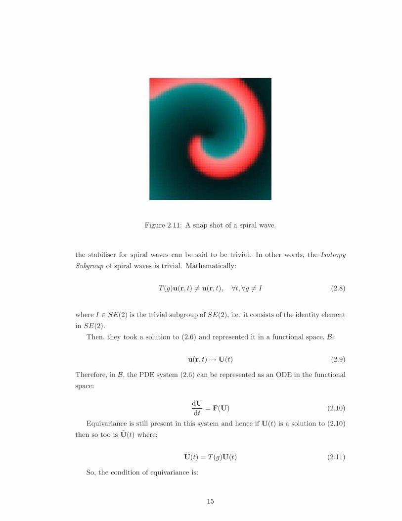
Figure 2.11: A snap shot of a spiral wave.
the stabiliser for spiral waves can be said to be trivial. In other words, the Isotropy
Subgroup of spiral waves is trivial. Mathematically:
T (g)u(r, t) 6= u(r, t), ∀t,∀g 6= I (2.8)
where I ∈ SE(2) is the trivial subgroup of SE(2), i.e. it consists of the identity element
in SE(2).
Then, they took a solution to (2.6) and represented it in a functional space, B:
u(r, t) 7→ U(t) (2.9)
Therefore, in B, the PDE system (2.6) can be represented as an ODE in the functional
space:
dU
dt= F(U) (2.10)
Equivariance is still present in this system and hence if U(t) is a solution to (2.10)
then so too is U(t) where:
U(t) = T (g)U(t) (2.11)
So, the condition of equivariance is:
15
T (g)F(U) = F(T (g)U(t))
for ∀U ∈ B and ∀g ∈ SE(2).
In the appendix, we provide the definition of an Group Orbit (Sec.(A.8.4)). In our
functional space, we take a solution, say V(t), and apply a particular transformation-
from SE(2) to this solution. This will give us our orbit. The orbit can therefore be
viewed as being fixed in time. Also, all spiral wave solutions along this orbit have the
same shape. If we took a solution along a particular orbit, then applying a transforma-
tion in SE(2) to this solution, we get another solution along this orbit. However, the
actual shape of the wave has not changed - only it’s position and orientation. The only
type of single armed spiral wave that corresponds to this situation is rigidly rotating
spiral waves.
So, what happens if we don’t travel along the orbits, but transversally to the orbits?
What we are observing in this case is that the wave is changing shape as we move across
the orbits. Therefore, we get Meandering Spiral Waves due to the shape of the wave
changing [54].
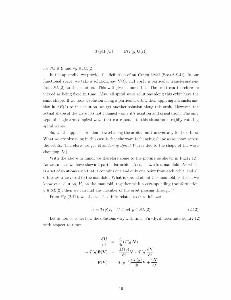
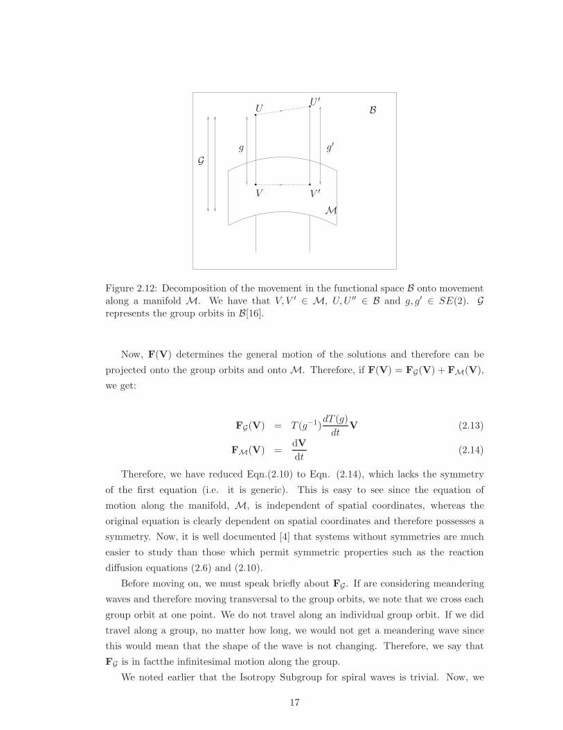
With the above in mind, we therefore come to the picture as shown in Fig.(2.12).
As we can see we have shown 2 particular orbits. Also, shown is a manifold,M which
is a set of solutions such that it contains one and only one point from each orbit, and all
orbitsare transversal to the manifold. What is special about this manifold, is that if we
know one solution, V , on the manifold, together with a corresponding transformation
g ∈ SE(2), then we can find any member of the orbit passing through V .
From Fig.(2.12), we also see that V is related to U as follows:
U = T (g)V, V ∈M, g ∈ SE(2) (2.12)
Let us now consider how the solutions vary with time. Firstly, differentiate Eqn.(2.12)
with respect to time:
dU
dt=
d
dt(T (g)V)
⇒ T (g)F(V) =dT (g)
dtV + T (g)
dV
dt
⇒ F(V) = T (g−1)dT (g)
dtV +
dV
dt
16
g
G
B
M
UU ′
V V ′
g′
Figure 2.12: Decomposition of the movement in the functional space B onto movementalong a manifold M. We have that V, V ′ ∈ M, U,U ′′ ∈ B and g, g′ ∈ SE(2). Grepresents the group orbits in B[16].
Now, F(V) determines the general motion of the solutions and therefore can be
projected onto the group orbits and onto M. Therefore, if F(V) = FG(V) + FM(V),
we get:
FG(V) = T (g−1)dT (g)
dtV (2.13)
FM(V) =dV
dt(2.14)
Therefore, we have reduced Eqn.(2.10) to Eqn. (2.14), which lacks the symmetry
of the first equation (i.e. it is generic). This is easy to see since the equation of
motion along the manifold, M, is independent of spatial coordinates, whereas the
original equation is clearly dependent on spatial coordinates and therefore possesses a
symmetry. Now, it is well documented [4] that systems without symmetries are much
easier to study than those which permit symmetric properties such as the reaction
diffusion equations (2.6) and (2.10).
Before moving on, we must speak briefly about FG . If are considering meandering
waves and therefore moving transversal to the group orbits, we note that we cross each
group orbit at one point. We do not travel along an individual group orbit. If we did
travel along a group, no matter how long, we would not get a meandering wave since
this would mean that the shape of the wave is not changing. Therefore, we say that
FG is in factthe infinitesimal motion along the group.
We noted earlier that the Isotropy Subgroup for spiral waves is trivial. Now, we
17
y
x
v1(x, y) = u10
v2(x, y) = u20
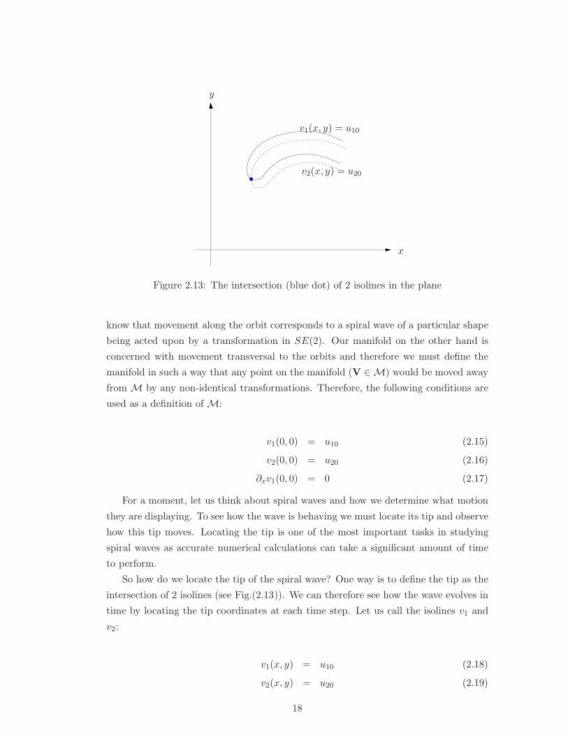
Figure 2.13: The intersection (blue dot) of 2 isolines in the plane
know that movement along the orbit corresponds to a spiral wave of a particular shape
being acted upon by a transformation in SE(2). Our manifold on the other hand is
concerned with movement transversal to the orbits and therefore we must define the
manifold in such a way that any point on the manifold (V ∈M) would be moved away
from M by any non-identical transformations. Therefore, the following conditions are
used as a definition of M:
v1(0, 0) = u10 (2.15)
v2(0, 0) = u20 (2.16)
∂xv1(0, 0) = 0 (2.17)
For a moment, let us think about spiral waves and how we determine what motion
they are displaying. To see how the wave is behaving we must locate its tip and observe
how this tip moves. Locating the tip is one of the most important tasks in studying
spiral waves as accurate numerical calculations can take a significant amount of time
to perform.
So how do we locate the tip of the spiral wave? One way is to define the tip as the
intersection of 2 isolines (see Fig.(2.13)). We can therefore see how the wave evolves in
time by locating the tip coordinates at each time step. Let us call the isolines v1 and
v2:
v1(x, y) = u10 (2.18)
v2(x, y) = u20 (2.19)
18
where u10 and u20 are arbitrary constants. Now u10 and u20 need to be chosen carefully
and in particular they must be located within the “No Mans Land” as described in [24],
otherwise a spiral wave may appear to have no tip by this definition.
Now, let us consider motion along the group orbit. We know, from the previous
section, that the equation of motion is given by Eqn.(2.13). Biktashev et al then showed
that by considering the motion along the group orbit we get:
FG(V) = −((c,∇) + ω∂θ)V (2.20)
for some c ∈ R2 and ω ∈ R.
Since F(V) = FG(V)+FM(V), then the movement along the manifold is FM(V) =
F(V)− FG(V).
Therefore, we get that in the PDE formulation, our reaction diffusion equation now
becomes:
FM(V) = F(V)− FG(V) (2.21)
⇒ dV
dt= F(V)− FG(V) (2.22)
⇒ ∂v
∂t= D∇2v + f(v) + (c,∇)v + ω∂θv (2.23)
So, what have we got in this case? Well, we now have a Reaction-Diffusion-
Advection equation of the motion along the manifold, with each solution v(r, t) being
located on the manifold. Therefore, the reaction diffusion equation is now in a comov-
ing frame of reference (with the origin located at the tip of the spiral wave) and not
a laboratory frame as in Eqn.(2.6). In Eqn.(2.23), we have that c and ω are changing
with time. Therefore, for each solution of Eqn.(2.23), v(r, t), we have a corresponding
unique value for c and ω. So by solving Eqn.(2.23), we can find each v, c and ω, for
each instant of time. Hence we can say that c and ω can be found by whatever method
we decide to use and so there exists a unique v, c, ω for each point on the manifold.
Also, since each c and ω change as each solution v(x, y, t) changes, then Eqn.(2.23)
together with Eqns.(2.15)-(2.17) can be viewed as a dynamical system. Finally, Eqns.
(2.15)-(2.17) can be viewed as the quotient system of the spiral wave solution to
Eqn.(2.23).
The next aim of the paper was to derive the equations of motion for the tip of the
wave. Their analysis produced the following relation:
T (cdt, ωdt) = id− dt(c,∇)− dtω∂θ (2.24)
19
where dt is the timestep. Also, by considering motion along the group orbit, i.e.
Eqn.(2.13), they were able to establish another relation:
T (R + dR,Θ + dΘ) = T (R,Θ)T (dtc, dtω) (2.25)
where dR and dΘ are infinitesimal shifts in R and Θ respectively. Therefore, by taking
Eqns.(2.24) and (2.25), and also considering,
T (g) : z 7→ R + zeγΘ (2.26)
where γ is the rotational matrix given by:
γ =
(
0 −11 0
)
then we have,
TR + dR,Θ + dΘz = TR,ΘTdtc, dtωz (2.27)
⇒ R + dR + eγ(Θ+dΘ)z = TR,Θ(dtc + eγdtωz) (2.28)
⇒ dR + eγΘeγdΘz = dteγΘc + eγdtωeγΘz (2.29)
which leads nicely to the equations of motion:
dR
dt= eγΘ(t)c(t) (2.30)
dΘ
dt= ω(t) (2.31)
or, using complex notation:
dR
dt= c(t)eiΘ(t) (2.32)
dΘ
dt= ω(t) (2.33)
It is easy that to see when we have rigid rotation, i.e. c and ω are constant, then
we can easily integrate Eqns.(2.32) and (2.33) to get:
20
R = R0 −ic
ωei(ωt+Θ0) (2.34)
where R = X + iY are the tip coordinates, R0 = X0 + iY0 is the initial position of the
tip of the wave, and c = cx + icy and ω are the translational and angular velocities. Of
course, Eqn.(2.34) is the equation of a circle, hence proving that the trajectory traced
out by the tip of a rigidly rotating spiral wave is a perfect circle.
Let us now consider meandering spiral waves. It is well documented that there are
2 frequencies present in a simple meandering spiral wave (again, we name just a few
of these for reference - [63], [11], [29], [47]). It has also be shown that the transition
from rigid rotation to meandering, is via a Hopf Bifurcation ([11], [36]). This Hopf
Bifurcation affects the motion of the wave by introducing a new frequency into the
system, the Hopf Frequency.
Biktashev et al proposed that the forms of c and ω should be derived straight from
Hopf Bifurcation Theory. They proposed to use the following form:
c(t) = c0 + c1z + c1z + O(|z|2) (2.35)
ω(t) = ω0 + ω1z + ω1z + O(|z|2) (2.36)
z = αz − βz|z|2 (2.37)
Therefore, using Eqns.(2.35) and (2.36), together with z = rei(ωH t+φ), we can inte-
grate Eqns.(2.32) and (2.33) directly to get:
R = R0 + A
(
sin(α)− cos(α)
)
+B
(
cos(α) − sin(α)sin(α) cos(α)
)(
m1 sin(β) + n2 cos(β)m2 sin(β)− n1 cos(β)
)
(2.38)
where:
21
α = ω0t + θ0 (2.39)
β = ωHt + φ (2.40)
A =c0
ω0(2.41)
B =2r
ωH(ω2H − ω2
0)(2.42)
c1 = c11 + ic12 (2.43)
ω1 = ω11 + iω12 (2.44)
m1 = ω2Hc11 − ω0c0ω11 (2.45)
m2 = ωH(c0ω12 − ω0c12) (2.46)
n1 = ωH(c0ω11 − ω0c11) (2.47)
n2 = ω2Hc12 − ω0c0ω12 (2.48)
Clearly, if there is no limit cycle present, i.e. r = 0, we get the equation of motion
for the rigidly rotating waves, since we will have that A = 0.
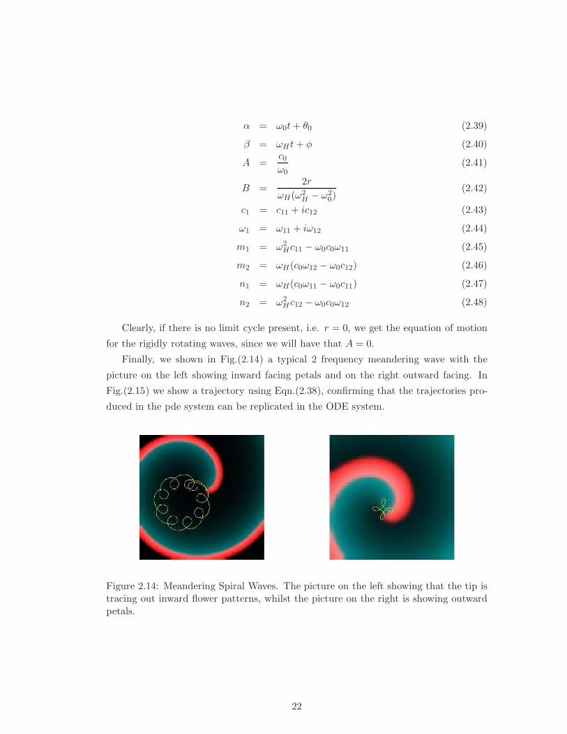
Finally, we shown in Fig.(2.14) a typical 2 frequency meandering wave with the
picture on the left showing inward facing petals and on the right outward facing. In
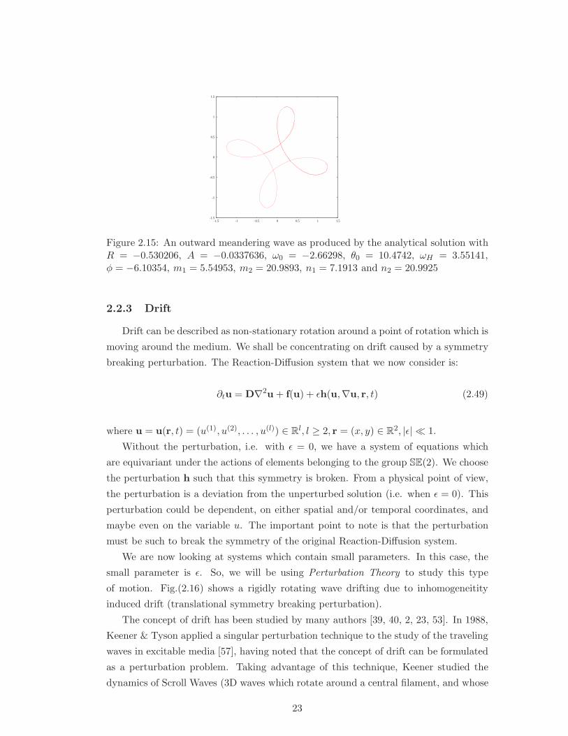
Fig.(2.15) we show a trajectory using Eqn.(2.38), confirming that the trajectories pro-
duced in the pde system can be replicated in the ODE system.
Figure 2.14: Meandering Spiral Waves. The picture on the left showing that the tip istracing out inward flower patterns, whilst the picture on the right is showing outwardpetals.
22
-1.5
-1
-0.5
0
0.5
1
1.5
-1.5 -1 -0.5 0 0.5 1 1.5
Figure 2.15: An outward meandering wave as produced by the analytical solution withR = −0.530206, A = −0.0337636, ω0 = −2.66298, θ0 = 10.4742, ωH = 3.55141,φ = −6.10354, m1 = 5.54953, m2 = 20.9893, n1 = 7.1913 and n2 = 20.9925
2.2.3 Drift
Drift can be described as non-stationary rotation around a point of rotation which is
moving around the medium. We shall be concentrating on drift caused by a symmetry
breaking perturbation. The Reaction-Diffusion system that we now consider is:
∂tu = D∇2u + f(u) + ǫh(u,∇u, r, t) (2.49)
where u = u(r, t) = (u(1), u(2), . . . , u(l)) ∈ Rl, l ≥ 2, r = (x, y) ∈ R
2, |ǫ| ≪ 1.
Without the perturbation, i.e. with ǫ = 0, we have a system of equations which
are equivariant under the actions of elements belonging to the group SE(2). We choose
the perturbation h such that this symmetry is broken. From a physical point of view,
the perturbation is a deviation from the unperturbed solution (i.e. when ǫ = 0). This
perturbation could be dependent, on either spatial and/or temporal coordinates, and
maybe even on the variable u. The important point to note is that the perturbation
must be such to break the symmetry of the original Reaction-Diffusion system.
We are now looking at systems which contain small parameters. In this case, the
small parameter is ǫ. So, we will be using Perturbation Theory to study this type
of motion. Fig.(2.16) shows a rigidly rotating wave drifting due to inhomogeneitity
induced drift (translational symmetry breaking perturbation).
The concept of drift has been studied by many authors [39, 40, 2, 23, 53]. In 1988,
Keener & Tyson applied a singular perturbation technique to the study of the traveling
waves in excitable media [57], having noted that the concept of drift can be formulated
as a perturbation problem. Taking advantage of this technique, Keener studied the
dynamics of Scroll Waves (3D waves which rotate around a central filament, and whose
23
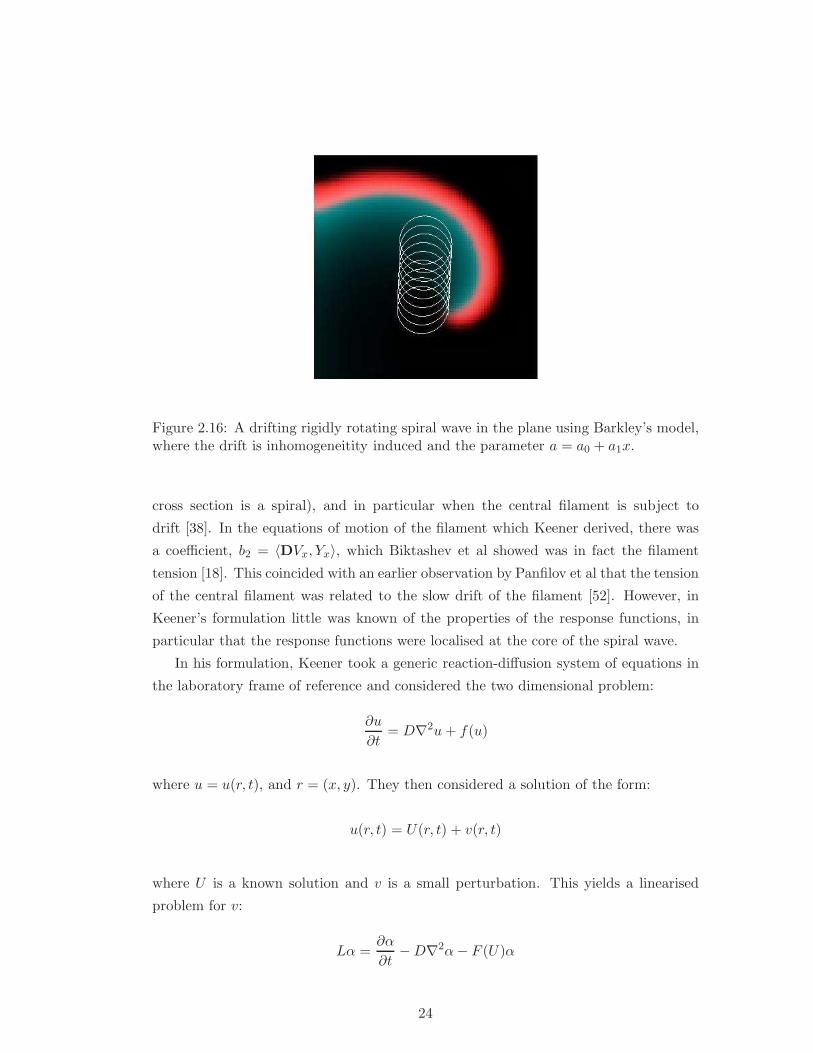
Figure 2.16: A drifting rigidly rotating spiral wave in the plane using Barkley’s model,where the drift is inhomogeneitity induced and the parameter a = a0 + a1x.
cross section is a spiral), and in particular when the central filament is subject to
drift [38]. In the equations of motion of the filament which Keener derived, there was
a coefficient, b2 = 〈DVx, Yx〉, which Biktashev et al showed was in fact the filament
tension [18]. This coincided with an earlier observation by Panfilov et al that the tension
of the central filament was related to the slow drift of the filament [52]. However, in
Keener’s formulation little was known of the properties of the response functions, in
particular that the response functions were localised at the core of the spiral wave.
In his formulation, Keener took a generic reaction-diffusion system of equations in
the laboratory frame of reference and considered the two dimensional problem:
∂u
∂t= D∇2u + f(u)
where u = u(r, t), and r = (x, y). They then considered a solution of the form:
u(r, t) = U(r, t) + v(r, t)
where U is a known solution and v is a small perturbation. This yields a linearised
problem for v:
Lα =∂α
∂t−D∇2α− F (U)α
24
where F (U) = ∂f(u)∂u|u = U . The corresponding adjoint linearised equation was:
L∗β =∂β
∂t+ D∇2β + F T (U)β
Therefore, we note that in this frame of reference, the critical eigenvalues are all
zero and that the eigenfunctions and response functions are all time dependent. The
inner product used by Keener therefore took the form:
〈u, v〉 = limr→∞
∫ P
0
∫ 2π
0
∫ r
0 u.vrdrdθdt
πr2P
In 1995, Biktashev et al used used a similar perturbation technique to produce a
theory of drift of a spiral wave [14]. We shall review this in detail in the next section.
However, we should note that Biktashev et al formulated their problem in a slightly
different way, making use of the conjecture that the response functions were localised.
This lead to a different formulation of the scalar product between the Goldstone modes
(eigenfunction to the linearised reaction-diffusion equation) and the response functions,
leading to a difference in the normalisation of the response functions. They also con-
sidered solutions in a rotating frame of reference, in which the rigidly rotating spiral
wave solutions are stationary.
Theory of Drift [14]
We shall review in some detail, the paper by Biktashev and Holden, published in
1995 on the theory of drift. Although the paper is entitled in such a way as to suggest
that only resonant drift is considered, it actually considers just a symmetry breaking
perturbation, with several excellent specific examples included for good measure.
They commence the theoretical work in this paper by considering the following
generic Reaction-Diffusion Equation (Eqn.(2.49)). They aimed to study spiral wave
solutions of (2.49) and therefore sought solutions of the form:
u = u(r, t) = u(ρ, θ + ωt) (2.50)
where r = (x, y) and ρ = ρ(r), θ = θ(r) are polar co-ordinates in the (x, y) plane. In
particular, we shall assume that the solution to (2.49) supports rigid rotation. This
means that ω is constant. Furthermore, they considered the unperturbed situation and
assumed that the solution to (2.49) is:
u = u0(r, t) = u0(ρ, θ + ωt) (2.51)
25
with u0 being 2π-periodic. This means that (2.49) becomes:
∂tu0 = D∇2u0 + f(u0) (2.52)
It is well known that spiral wave solutions to (2.49) with no perturbation are in-
variant under euclidean symmetry as well temporal transformations. This implies that
(2.51) is a solution to (2.49) with ǫ = 0 then so too is:
u0;δr,δt = u0(r− δr, t− δt) (2.53)
It can therefore be said that equation (2.53) generates a 3 dimensional manifold of
solutions to (2.49).
Also, since they know considered a rigidly rotating spiral waves, then the solution
is stable. This means that any small deviation away from the solution eventual ends
up in a small vicinity of the unperturbed solution. Hence we arrive at the following
Stability Postulate:
Stability Postulate: Any solution to (2.49) at ǫ = 0 with initial conditions sufficiently
close to (2.50) tends to one of the solutions to (2.53) with some δr, δt as t → ∞, i.e.
the family (2.53) is stable as a whole against small perturbations in initial conditions.
They firstly considered the system of solutions to (2.49) with ǫ = 0 and also with a
perturbation present in the solution. A small deviation in the solution could arise from
a small deviation in the initial conditions. It was assumed that the solution to (2.49)
is of the form:
u = u0(r, t) + v(r, t) = u0(ρ, θ + ωt) + v(r, t) (2.54)
where v(r, t) = O(ǫ) is the perturbation. Therefore, the initial conditions are:
u(r, 0) = u0(r, 0) + v0(r) (2.55)
Substituting (2.54) into (2.49) and splitting out unperturbed from perturbed parts,
we get:
∂u0
∂t= D∇2u0 + f(u0) (2.56)
∂v
∂t= Lv (2.57)
where linearised operator L is given by:
26
Lα = D∇2α +∂f
∂uα (2.58)
We see that Eqn.(2.57) is the equation of motion for the small perturbation from
the original solution. v(r, t) can be thought of as the remainder terms if we are using
Asymptotic Methods. Since they considered rigidly rotating spiral waves, it is more
convenient to perform the analysis in a rotating frame of reference, i.e.:
t → t = t
r → r : ρ(r) = ρ(r), θ(r) = θ(r) + ωt
Hence, (2.57) becomes:
∂v
∂t= Lv (2.59)
where:
Lv = D∇2v + vF(u0(r))− ω∂v
∂θ(2.60)
Now, it was noted that the study of the linear stability of the operator, L, by
studying the eigenvalues and eigenvectors of the linear system. It is well known that
there are three critical eigenvalues who have with zero real parts for rigidly rotating
spiral waves. These come from the symmetry of the unperturbed system. So, it can be
said that the solution (2.51) differs from (2.53) at small δr and δt by a function linearly
composed of three linearly independent functions.
They then considered the eigenfunctions to the linear operator L, and, after some
analysis, it can be shown that these take the form:
V0 = −ω∂u0
∂θ, λ0 = 0 (2.61)
V1 = −1
2
(
∂u0
∂ρ− i
1
ρ
∂u0
∂θ
)
e−iθ, λ1 = iω (2.62)
V−1 = −1
2
(
∂u0
∂ρ+ i
1
ρ
∂u0
∂θ
)
eiθ, λ−1 = −iω (2.63)
Accordingly to the stability postulate, there should be no other eigenvalues on the
imaginary axis. So, the solution to (2.59) can be expanded in its eigenbasis as follows:
v(r, t) = c0V0(r) + c1eiωtV1(r) + c−1e
−iωtV−1(r) + o(1) (2.64)
27
as t→∞. To determine the coefficients ci, they took the scalar product of (2.64) with
the eigenfunctions to the adjoint operator L+ to get:
c0,±1 = (W0,±iω, v) (2.65)
where W0,±iω satisfies:
L+W0,±iω = λ0,±iωW0,±iω (2.66)
and the following orthogonality condition holds:
(Wi, Vj) = δij (2.67)
Now, the scalar products used above are the scalar products in a functional space
and defined as:
(W,V ) =
∫ ∫
〈W (r), V (r)〉d2r (2.68)
where the integration is over the whole plane.
They then considered the case for ǫ 6= 0, and firstly considered a regular perturba-
tion technique.
u(r, t) = u0(r, t) + ǫv(r, t) + O(ǫ2) (2.69)
In the rotating frame of reference, we get:
∂v
∂t= Lv + h(u0(r), r, t) (2.70)
which is similar to Eqn.(2.59) but with the perturbation term added. It was then
assumed that the solution to (2.70) can be expressed as the linear combination of its
eigenvectors and eigenvalues, and in particular that its eigenvectors form the span of
solutions in the space of solutions:
v(t) =∑
λ
ci(t)Vi (2.71)
where Vi are the eigenvectors of the linearised system (2.71). It was noted that v is a
28
function of t and therefore, since Vi is a vector constant, hence ci = ci(t). They then
needed to find expressions for ci.
This can then be written as:
v(t) =∑
λ
Vieλt
∫ t
0e−λτH(τ)dτ (2.72)
In the knowledge that there are 3 eigenvalues with values 0,±iω. They then consid-
ered the case when λ = 0. They then showed that (Wj , v) = cj = eλt∫ t
0 e−λτH(τ )dτ ,
noting that j is the eigenvalue. Therefore, when λ = 0:
(W0, v) =
∫ t
0H(τ)dτ (2.73)
⇒ (W0, v) =
∫ t
0(W0, h)dτ (2.74)
Now, as t→∞, they found that (2.74) grows to infinity, if, for example, they had
that (W0, h) is a non-zero constant.
So, what does all this mean? Well, we have seen that if we have small perturbation,
then as t → ∞ the functions ci become very large. This in term means that v(t) also
becomes large and therefore contradicts the stability postulate of a previous section.
Hence, we can say that the Regular Perturbation technique implemented here does
not work and so cannot describe drift. Therefore, Biktashev et al decided to look at
Singular Perturbation methods.
They then decided to use a singular perturbation technique to study this particular
system. This allowed to obtain solutions that are valid for large values of time at
bounded values of h. They therefore considered solutions of the form:
u(r, t) = u0
(
r−R(t), t− Φ(t)
ω
)
+ ǫv(r, t) (2.75)
= u0(ρ(r−R(t)), θ(r−R(t)) + ωt− Φ(t)) + ǫv(r, t) (2.76)
By using similar techniques to the regular perturbation theory, they established theequation for v:
ǫ∂tv = ǫLv + ǫh
„
u0
„
r− R, t −Φ
ω
«
, r, t
«
+ ∂θu0
„
r− R, t −Φ
ω
«
+∂xu0
„
r − R, t −Φ
ω
«
X′(t) + ∂yu0
„
r− R, t −Φ
ω
«
Y′(t) + O(ǫ) (2.77)
In a frame of reference associated with the spiral wave, they got:
ǫ∂tv = ǫLv + ǫh (u0(r), r, t) +1
ωV0(r)Φ
′(t)
+(
V1(r)ei(ωt−Φ) + V−1(r)e
−i(ωt−Φ))
X ′(t)
+(
iV1(r)ei(ωt−Φ) − iV−1(r)e
−i(ωt−Φ))
Y ′(t) + O(ǫ) (2.78)
29
Therefore, by taking the scalar product of Eqn.(2.78) with the eigenfunctions to the
adjoint operator L+, we have:
Φ′(t) = ǫω(W0, h) + O(ǫ) (2.79)
X ′(t) = ǫReei(ωt−Φ)(W1,h)+ O(ǫ) (2.80)
Y ′(t) = ǫImei(ωt−Φ)(W1,h)+ O(ǫ) (2.81)
Therefore, they have obtained the equations of motion along the manifold (2.53) under
a generic perturbation h(u, r, t).
They then considered two examples; Resonant drift, where the perturbation is time
dependent only; and Inhomogeneitity induced drift. We will review the simpler example
in this thesis, which is Resonant drift.
So, consider a perturbation of the form:
h(u, r, t) = H(Ωt− φ), such that H(φ + 2π) = H(φ) (2.82)
Next, we shall consider the averaged motion of the spiral. Therefore, the equations
of motion (2.79)-(2.81), become:
Φ′(t) = ǫH0 + O(ǫ) (2.83)
X ′(t) = ǫ|H1| cos((ωt − Φ)− (Ωt− φ) + argH1) + O(ǫ) (2.84)
Y ′(t) = ǫ|H1| sin((ωt− Φ)− (Ωt− φ) + argH1) + O(ǫ) (2.85)
where Hn are given by:
Hn =
∫ ⟨∫
Wnd2r,H(η)
⟩
e−inηdη (2.86)
Introducing the notation:
ϕ = (ωt − Φ)− (Ωt− φ) + argH1 (2.87)
we get:
φ′(t) = ω + ǫH0 − Ω + O(ǫ) (2.88)
X ′(t) = ǫ|H1| cos(φ) + O(ǫ) (2.89)
Y ′(t) = ǫ|H1| sin(φ) + O(ǫ) (2.90)
which, when integrated, give us the equation of a circle.
30
2.3 Models used in Numerical Analysis
In our numerical work, we will be using two models - the FitzHugh-Nagumo model
[24, 49], affectionately known as FHN, and Barkley’s model [11, 8]. Barkley’s model is
shown below
∂u(1)
∂t= ∇2u(1) +
1
εu(1)(1− u(1))
[
u(1) − u(2) + b
a
]
(2.91)
∂u(2)
∂t= Dv∇2u(2) + u(1) − u(2) (2.92)
where a, b, and ε are parameters, and also u(i) represents the i’th component of the two
component system. In his original papers [11, 8], Barkley calls u(1) = u and u(2) = v,
but we will try to be consistent with notation throughout this thesis and therefore we
adopt our notation as shown in (2.91).
FHN on the other hand, is similar to Barkley’s model but takes a slightly different
form:
∂u(1)
∂t= ∇2u(1) +
1
ε
(
u(1) − (u(1))3
3− u(2)
)
(2.93)
∂u(2)
∂t= Dv∇2u(2) + ε
(
u(1) + β − γu(2))
(2.94)
where the parameters in this model are β, γ and ε.
It must be stressed at this stage that ε in these models are not necessarily small
quantities, unlike the ǫ that we will be using in Perturbation Theory. They are model
parameters and in fact determine the slow and fast times within the models. In most
cases they are taken to be small, but they must not get confused with the small pa-
rameters used in perturbation theory.
2.3.1 Similarities in the FHN and Barkley’s Models
There are many similarities between the two models. For instance, in the evolution
of the u(1) fields, both models have cubic local kinetics. Also in the u(2) fields, the local
kinetics are linear.
They also have very similar phase portraits as shown in Figs.(2.17) and (2.18).
For FHN, the nullclines are given by:
l1 : u(2) =1
γu(1) +
β
γ(2.95)
l2 : u(2) = u(1) − (u(1))3
3(2.96)
31

u(2)
u(1)10
l1
l2
Figure 2.17: Barkley’s model:Phase Portrait.
u(2)
u(1)
l1
l2
Figure 2.18: FHN model:Phase Portrait.
whereas in Barkley they are:
horizontal nullclines : u(2) = u(1) (2.97)
vertical nullclines : u(2) = au(1) − b, u(1) = 0, u(1) = 1 (2.98)
Also we have that the intersections of the nullclines occur at (0, 0) & (±√
3, 0) in
FHN, and at (0.0) & (1, 1) in Barkley’s model.
In both phase portraits, we have detailed not only typical excitation trajectories
(given in blue) but have also shown the directions of the trajectories throughout the
portrait given by the red arrows. We have tried to use the length of these directional
arrows to indicate the speed of the trajectory at those points; so a short arrow would
indicate a slow speed, etc.
In each case, the stable fixed point is shown by a large black dot, and is located
at (0, 0) in Barkley’s model and (xS , yS) in FHN where xS and yS are the coordinates
of the intersection of the two isolines. Just thinking about the steady state in FHN,
this state always depends on the values of the model parameters, β and γ. However,
in Barkley’s model, the stable steady state is fixed, no matter what the values of the
model parameters.
We can also go as far to say that Barkley’s model is just a simplified version of the
FHN model. Consider the vertical nullclines. In Barkley’s model, two of these nullclines
form the vertical lines of a backward “N” shape. These are the “slow” nullclines,
meaning that the trajectory moves slowly along with respect to these nullclines, with
the horizontal nullcline being the fast nullcline. The middle part of the “N” shape, is
32
u(2)
u(1)
10
δ
l1
l2
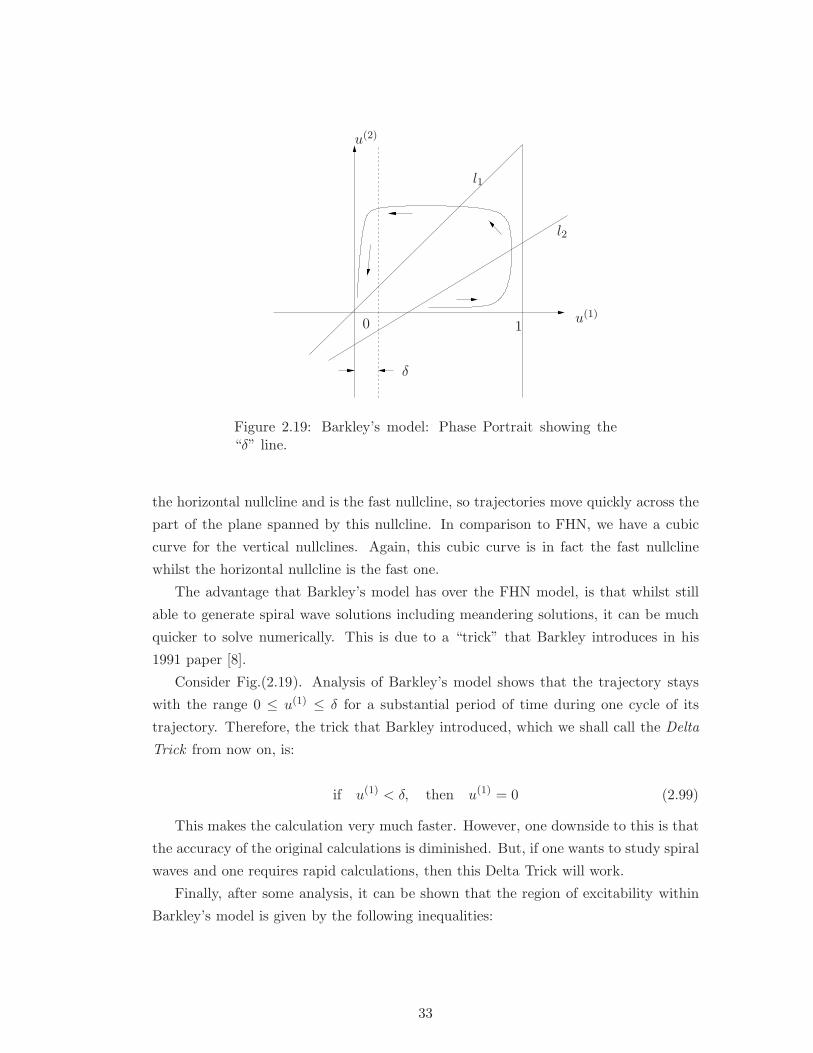
Figure 2.19: Barkley’s model: Phase Portrait showing the“δ” line.
the horizontal nullcline and is the fast nullcline, so trajectories move quickly across the
part of the plane spanned by this nullcline. In comparison to FHN, we have a cubic
curve for the vertical nullclines. Again, this cubic curve is in fact the fast nullcline
whilst the horizontal nullcline is the fast one.
The advantage that Barkley’s model has over the FHN model, is that whilst still
able to generate spiral wave solutions including meandering solutions, it can be much
quicker to solve numerically. This is due to a “trick” that Barkley introduces in his
1991 paper [8].
Consider Fig.(2.19). Analysis of Barkley’s model shows that the trajectory stays
with the range 0 ≤ u(1) ≤ δ for a substantial period of time during one cycle of its
trajectory. Therefore, the trick that Barkley introduced, which we shall call the Delta
Trick from now on, is:
if u(1) < δ, then u(1) = 0 (2.99)
This makes the calculation very much faster. However, one downside to this is that
the accuracy of the original calculations is diminished. But, if one wants to study spiral
waves and one requires rapid calculations, then this Delta Trick will work.
Finally, after some analysis, it can be shown that the region of excitability within
Barkley’s model is given by the following inequalities:
33
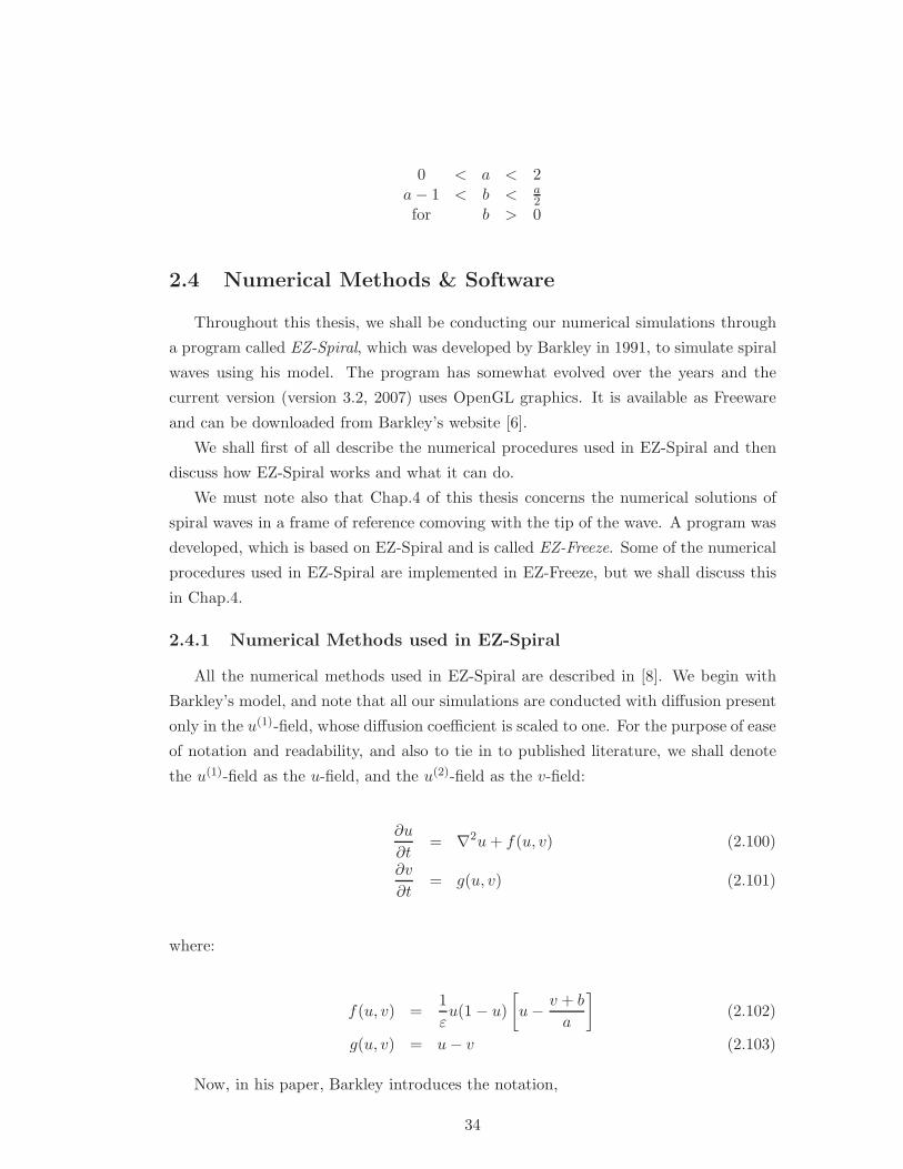
0 < a < 2a− 1 < b < a
2for b > 0
2.4 Numerical Methods & Software
Throughout this thesis, we shall be conducting our numerical simulations through
a program called EZ-Spiral, which was developed by Barkley in 1991, to simulate spiral
waves using his model. The program has somewhat evolved over the years and the
current version (version 3.2, 2007) uses OpenGL graphics. It is available as Freeware
and can be downloaded from Barkley’s website [6].
We shall first of all describe the numerical procedures used in EZ-Spiral and then
discuss how EZ-Spiral works and what it can do.
We must note also that Chap.4 of this thesis concerns the numerical solutions of
spiral waves in a frame of reference comoving with the tip of the wave. A program was
developed, which is based on EZ-Spiral and is called EZ-Freeze. Some of the numerical
procedures used in EZ-Spiral are implemented in EZ-Freeze, but we shall discuss this
in Chap.4.
2.4.1 Numerical Methods used in EZ-Spiral
All the numerical methods used in EZ-Spiral are described in [8]. We begin with
Barkley’s model, and note that all our simulations are conducted with diffusion present
only in the u(1)-field, whose diffusion coefficient is scaled to one. For the purpose of ease
of notation and readability, and also to tie in to published literature, we shall denote
the u(1)-field as the u-field, and the u(2)-field as the v-field:
∂u
∂t= ∇2u + f(u, v) (2.100)
∂v
∂t= g(u, v) (2.101)
where:
f(u, v) =1
εu(1− u)
[
u− v + b
a
]
(2.102)
g(u, v) = u− v (2.103)
Now, in his paper, Barkley introduces the notation,
34
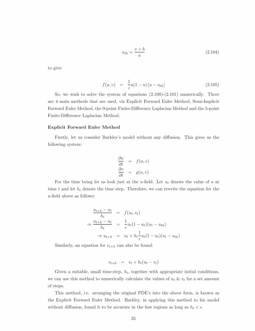
uth =v + b
a(2.104)
to give:
f(u, v) =1
εu(1− u) [u− uth] (2.105)
So, we wish to solve the system of equations (2.100)-(2.101) numerically. There
are 4 main methods that are used, viz Explicit Forward Euler Method, Semi-Implicit
Forward Euler Method, the 9-point Finite-Difference Laplacian Method and the 5-point
Finite-Difference Laplacian Method.
Explicit Forward Euler Method
Firstly, let us consider Barkley’s model without any diffusion. This gives us the
following system:
∂u
∂t= f(u, v)
∂v
∂t= g(u, v)
For the time being let us look just at the u-field. Let ut denote the value of u at
time t and let ht denote the time step. Therefore, we can rewrite the equation for the
u-field above as follows:
ut+h − ut
ht= f(ut, vt)
⇒ ut+h − ut
ht=
1
ǫut(1− ut)(ut − uth)
⇒ ut+h = ut + ht1
ǫut(1− ut)(ut − uth)
Similarly, an equation for vt+h can also be found:
vt+h = vt + ht(ut − vt)
Given a suitable, small time-step, ht, together with appropriate initial conditions,
we can use this method to numerically calculate the values of ut & vt for a set amount
of steps.
This method, i.e. arranging the original PDE’s into the above form, is known as
the Explicit Forward Euler Method. Barkley, in applying this method to his model
without diffusion, found it to be accurate in the fast regions as long as ht < ǫ.
35
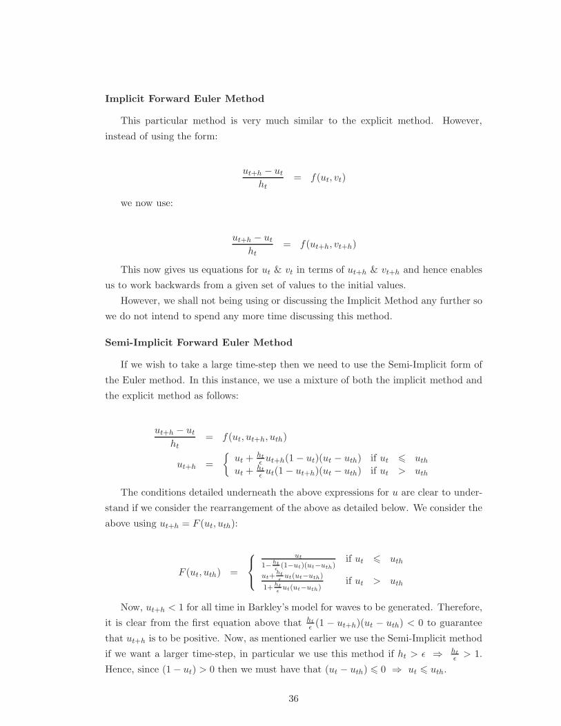
Implicit Forward Euler Method
This particular method is very much similar to the explicit method. However,
instead of using the form:
ut+h − ut
ht= f(ut, vt)
we now use:
ut+h − ut
ht= f(ut+h, vt+h)
This now gives us equations for ut & vt in terms of ut+h & vt+h and hence enables
us to work backwards from a given set of values to the initial values.
However, we shall not being using or discussing the Implicit Method any further so
we do not intend to spend any more time discussing this method.
Semi-Implicit Forward Euler Method
If we wish to take a large time-step then we need to use the Semi-Implicit form of
the Euler method. In this instance, we use a mixture of both the implicit method and
the explicit method as follows:
ut+h − ut
ht= f(ut, ut+h, uth)
ut+h =
ut + ht
ǫut+h(1− ut)(ut − uth) if ut 6 uth
ut + ht
ǫut(1− ut+h)(ut − uth) if ut > uth
The conditions detailed underneath the above expressions for u are clear to under-
stand if we consider the rearrangement of the above as detailed below. We consider the
above using ut+h = F (ut, uth):
F (ut, uth) =
ut
1−htǫ
(1−ut)(ut−uth)if ut 6 uth
ut+htǫ
ut(ut−uth)
1+htǫ
ut(ut−uth)if ut > uth
Now, ut+h < 1 for all time in Barkley’s model for waves to be generated. Therefore,
it is clear from the first equation above that ht
ǫ(1 − ut+h)(ut − uth) < 0 to guarantee
that ut+h is to be positive. Now, as mentioned earlier we use the Semi-Implicit method
if we want a larger time-step, in particular we use this method if ht > ǫ ⇒ ht
ǫ> 1.
Hence, since (1− ut) > 0 then we must have that (ut − uth) 6 0 ⇒ ut 6 uth.
36
A similar argument is used to show the second condition. Again, we require ut+h >
0. This therefore means that the denominator is positive. Hence, to guarantee this
condition, we need that ht
ǫut(ut − uth) > 0. Now, ht
ǫ> 0 and ut > 0 hence ut − uth >
0 ⇒ ut > uth.
To summarise for the Euler Methods, we can see that for small ht
ǫ, we use the
Explicit Method (note that the Explicit method can be derived from the expressions
for the Semi-Implicit method by expanding the denominators in the expressions for
F (ut, uth) above). For large ht
ǫ, we need to use a Semi-Implicit Method and find that
we can simplify the expressions for F (ut, uth) as follows:
F (ut, uth) = 0 if ut < uth
= uth if ut = uth
= 1 if ut > uth
Five-Point and Nine-Point Finite-Difference Laplacian Method
The Forward Euler Methods as described above efficiently solve the system, numer-
ically, in the absence of diffusion. Therefore, we now need to introduce a scheme which
looks after the diffusion term.
We will use two schemes. The five-point scheme:
∇2un,m =un−1,m + un+1,m + un,m−1 + un,m+1 − 4un,m
h2x
+ O(h3x) (2.106)
and the nine-point scheme:
∇2un,m =1
h2x
(4 (un−1,m + un+1,m + un,m−1 + un,m+1) + un−1,m−1
+un+1,m−1 + un−1,m+1 + un−1,m+1 − 20un,m) + O(h3x) (2.107)
We note that both the five-point and nine-point schemes are second order accurate
schemes and therefore whether we use a five-point scheme or a nine-point scheme makes
no difference to the accuracy of the calculations.
Therefore, for the numerical work that we cover here, we shall be using the five-point
scheme, unless stated otherwise.
Operator Splitting
Another method used in the numerical schemes is operator splitting. The user of
EZ-Spiral has the choice as to whether they wish to use operator splitting or not. Let
us assume the evolution of the u-field takes the following form:
37
∂u
∂t= R(u, v) +D(u) (2.108)
where R is the reaction terms (f(u, v) in Barkley’s model) and D is the diffusion term.
If operator splitting is used then for each step then the equation above can be solved
as:
un+ 12
= un + htR(un, vn) (2.109)
un+1 = un+ 12
+ htD(un+ 12) (2.110)
where un is the current time step, un+1 is the next time step and un+ 12
is the half step
between the current step and the next step.
We shall be using operator splitting in the schemes we use in Chap.4.
2.4.2 EZ-Spiral
We shall now provide some details on the program EZ-Spiral which solves Barkley’s
model using the above mentioned numerical schemes. However, it doesn’t just solve it,
it also provides a graphical interpretation of the data which it has generated.
The program is written in C. It has been made available as Freeware software on
an open license from GNU. Users are encouraged to not only use the software for their
research but to amend it as they feel fit.
The graphics, in the latest version, is provided through OpenGL and we shall be
using the graphics part of the code within EZ-Spiral for the graphics in our own program
EZ-Freeze.
The program is aimed at Linux/Unix based systems and therefore the graphical
window is provided using X-Windows. The program can be run in non-graphical mode
in MS Windows, but obviously, only data can be generated, not graphics.
Provided with the program files is a file called task.dat. Within this file are a
variety of parameters, including the model parameters, numerical parameters, and a
variety of other parameters such as a parameter which determines whether a file is to be
produced containing the tip coordinates, or a parameter which determines how much
information is relayed to the user on the screen before, during and after the simulation.
The purpose of providing this file is so that we can compile the program just once and
if we need to amend any parameters, we can just do it easily through the task.dat file
and not through the code, thereby avoiding having to compile the program again.
38
So, once the program is made and is executed, an X-Window will appear. The
simulation is then started by activating the X-Window (by either clicking in the window
or hovering the mouse arrow over the window) and then pressing the space bar. Using
the parameters provided with the program when it is first downloaded, the user should
see a wave rotating fairly fast (depending on the spec of the system being used).
A variety of key presses are provided with the program. We have come across
space. Another is p, which pauses the simulation and q quits the simulation. Once the
simulation has been terminated using the q key, then a final conditions file is generated
containing a host of various bits of information, such as parametersused, and more
importantly, the values of u and v for each grid point at the tip the program was
terminated. The file produced is called fc.dat. This file can be copied to an initial
conditions file, ic.dat, and the next simulations start from those initial conditions.
Other key presses that are important are t and the arrow keys. The t key switches
tip plotting on and off. So, if we switch on tip plotting, then the tip trajectory will be
plotted on the screen from the moment t is pressed. The arrow keys moves the wave
around the screen screen.
One other point to note is that the code is extremely well commented. So it is not
hard for someone fluent in C to find their way around the code.
39
Chapter 3
Asymptotic Theory of Drift andMeander
3.1 Introduction
The aim of this chapter is to provide an asymptotic theory of the drift of meandering
spiral waves. Other authors have also worked on this area [44, 43, 64, 28], but we
provide an alternative approach to this subject and an approach which we think is
more straightforward.
We shall base our theory on the papers that were described in detail in Chap.2 -
the theory of meander [16] and the theory of drift [14]. Both theories were written
using different techniques and we intend to rewrite one of the theories using similar
techniques to those used in the other theory.
So, the first section of this chapter is devoted to the rewriting of the theory of
drift using group theoretical approaches as well as perturbation techniques. We will
concentrate, firstly, on a rigidly rotating spiral wave, and provide three examples of drift
(Resonant Drift, Electrophoretic Induced Drift, and Inhomogeneity Induced Drift).
We will then proceed to extend this theory to meandering spiral waves. We note
that in a suitable functional space (in this case the functional space will be the space
of all group orbits), the solutions are periodic. In fact they are limit cycle solutions.
This has been proven numerically, with attempts to prove it analytically by proving
the transition from rigid rotation to meander is via a Hopf bifurcation[64]. Therefore,
we shall be using Floquet theory to study the meandering part of the wave.
So, we will give a review of Floquet theory as first presented in 1883 by Gaston
Floquet [25], extending this to adjoint solutions, before applying Floquet theory to
meandering spiral waves. One of the features of the theory we will be presenting, is
that the singular perturbation method developed gives rise to an ODE which determines
the shift in the limit cycle. The solution to this ODE can be put into the form of the
40
Arnol’d Standard Mapping. Therefore, it is thought that frequency locking within
meandering spiral waves which are drifting due to symmetry breaking perturbations
can be observed.
We end the chapter with a conclusion and indication of further work to do in this
area.
3.2 Drift of a Rigidly Rotating Spiral Wave
3.2.1 Formulation of the problem
In this section, we present a study of the drift of a rigidly rotating spiral wave. We
will take a general Reaction-Diffusion system of equations (RDS) in the plane which
is subject to a symmetry breaking perturbation, and we apply perturbation and group
theory techniques to develop a theory that will describe the dynamics of the spiral
wave.
The system of equations we consider is shown below:
∂u
∂t= D∇2u + f(u) + ǫh(u,∇u, r, t), u, f,h ∈ R
n, D ∈ Rn×n r ∈ R
2 (3.1)
where u = u(r, t) = u(x, y, t) = (u(1), u(2), . . . , u(n), D is the matrix of diffusion coeffi-
cients, 0 < ǫ≪ 1 and n ≥ 2. If h = 0, then we have that Eqn.(3.1) is equivariant with
respect to Euclidean transformations of the plane.
The perturbation, h, could in practice be any perturbation, but for our purpose,
we require it to be a symmetry breaking perturbation and also that it is bounded.
Therefore, we have that Eqn.(3.1) is no longer equivariant under Euclidean symmetry.
We will later on show three distinct examples using different perturbations of how our
theory will work.
Now, we will be studying the spiral wave in a frame of reference that is moving
with the tip of the wave. There are several advantages to doing this, including the
derivation of a generic form of the equations of motion of the tip of the spiral wave
from the analysis in transforming the laboratory frame of reference to the comoving
frame. Therefore, we will need to define the tip of the wave in the comoving frame of
reference as follows:
u(i)(R, t) = u∗ (3.2)
u(j)(R, t) = v∗ (3.3)
∂u(i)
∂x(R, t) = 0 (3.4)
41
where R = (X,Y ) is the coordinate of the tip of the spiral wave in the (x, y) plane, and
1 ≤ i, j ≤ n. Also, we note that (3.4) is a derivative with respect to x and not x. Now,
x is the transformed laboratory frame coordinate, x, to the comoving frame given as:
(
xy
)
7→(
xy
)
=
(
cos(Θ) sin(Θ)− sin(Θ) cos(Θ)
)(
x−Xy − Y
)
where (X,Y ) are the tip coordinates and Θ is the tip phase. Therefore, our tip condi-
tions in the laboratory frame of reference now become:
u(i)(R, t) = u∗
u(j)(R, t) = v∗
cos(Θ)∂u(i)
∂x(R, t)− sin(Θ)
∂u(i)
∂y(R, t) = 0
Let us now define v(r, t) such that v(r, t) is a transformation of the solution u(r, t)
so that the tip of the wave is located at the origin for all time, and also the phase of the
tip of the wave is constant for all time. Therefore, we have that v(r, t) is the solution
to a RDS which is in the frame of reference moving with the tip of the wave. In the
next section, we will derive the RDS in the moving frame of reference.
Now, we define v such that it is related to u as follows:
v(r, t) = T (g−1)u(r, t)
⇒ u(r, t) = T (g)v(r, t)
where g ∈ SE(2), g = R,Θ, i.e. the group of all rotations and translations. T (g) is
the action of the group element g ∈ SE(2) and is defined as:
T (g)u(r, t) = u(g−1r, t)
Now, we will be choosing R and Θ such that they are the tip coordinates and phase.
We note that if (x, y) are the coordinates in the moving frame of reference, then:
(
xy
)
=
(
cos(Θ) sin(Θ)− sin(Θ) cos(Θ)
)(
x−Xy − Y
)
Clearly, we can see that in the moving frame of reference, Eqns.(3.2)-(3.4) become:
42
v(i)(0, t) = u∗ (3.5)
v(j)(0, t) = v∗ (3.6)
∂v
∂x
(i)
(0, t) = 0 (3.7)
where v(i) and v(j) are the i’th and j’th components of v respectively, and 1 ≤ i, j ≤ n,
and we have taken the tip to be at the origin.
As we will see in the next section, by representing this system in a functional space
we can rewrite it in the comoving frame of reference whose origin is located at the tip
of the spiral wave.
3.2.2 Representation in the comoving frame of reference
We now represent Eqn.(3.1) in a functional Space, B. The functional space in
question is taken to be the space of all Euclidean group orbits. A formal construction
of this space is found in [64].
We therefore find that the RDS in this space is:
dU
dt= F(U) + ǫH(U, t) (3.8)
where U,F,H ∈ B, and U(t)↔ u(x, t), F(U)↔ f(u) +∇2u.
Next, we define a manifold, which we call a Representative Manifold, in B consisting
of all functions which have the tip of the spiral wave at the origin of the frame of
reference for all time. We restrict our attention to spiral wave solutions, which may be
formally defined as those having just one tip. We also restrict the solutions to those
spiral waves having just one arm. Let us denote such a set of solutions S ⊂ B. So,
M : ∀U ∈ S, ∃′g ∈ SE(2),V ∈M : U = T (g)V
We will also assume that the set S with respect to (3.1) is open and invariant, i.e.
spiral waves do not terminate spontaneously and do not break up into many spirals (if
they do, then such behaviour is not either drift or meander, and is not considered by
this theory).
We can decompose the motion in this space as motion along the Representative
Manifold and motion along a group orbit which is transversal to this Representative
Manifold. We show in Fig.(3.1) the representative manifold and also a spiral wave
solution.
43
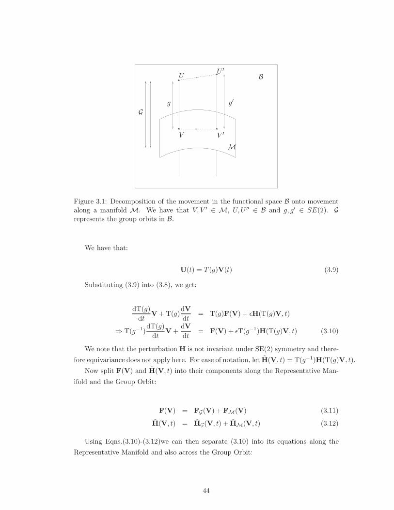
g
G
B
M
UU ′
V V ′
g′
Figure 3.1: Decomposition of the movement in the functional space B onto movementalong a manifold M. We have that V, V ′ ∈ M, U,U ′′ ∈ B and g, g′ ∈ SE(2). Grepresents the group orbits in B.
We have that:
U(t) = T (g)V(t) (3.9)
Substituting (3.9) into (3.8), we get:
dT(g)
dtV + T(g)
dV
dt= T(g)F(V) + ǫH(T(g)V, t)
⇒ T(g−1)dT(g)
dtV +
dV
dt= F(V) + ǫT(g−1)H(T(g)V, t) (3.10)
We note that the perturbation H is not invariant under SE(2) symmetry and there-
fore equivariance does not apply here. For ease of notation, let H(V, t) = T(g−1)H(T(g)V, t).
Now split F(V) and H(V, t) into their components along the Representative Man-
ifold and the Group Orbit:
F(V) = FG(V) + FM(V) (3.11)
H(V, t) = HG(V, t) + HM(V, t) (3.12)
Using Eqns.(3.10)-(3.12)we can then separate (3.10) into its equations along the
Representative Manifold and also across the Group Orbit:
44
dV
dt= FM(V) + ǫHM(V, t) Manifold (3.13)
T(g−1)dT(g)
dtV = FG(V) + ǫHG(V, t) Group Orbit (3.14)
Eqn.(3.13) can now be rewritten as follows using Eqns.(3.11) and (3.12):
dV
dt= F(V)− FG(V) + ǫH(V, t)− ǫHG(V, t)
Using the equation along the Group Orbit (3.14) together with Eqn.(3.9), we can
determine the generic forms of HG(V, t) and FG(V).
To do this, we must first establish the generic forms of the equations of motion along
the group orbits. Note that the representative manifold is made of spiral with their tip
at the origin. Thus, the group transformations describe the position and orientation of
the tip in the laboratory frame of reference.
3.2.3 Generic Forms of the Equations of Motion
Firstly, we consider the motion along the group orbit as given by Eqn.(3.14) and, in
particular, the form of the left hand side of this particular equation. We shall consider
how the operator T(g−1)dT(g)dt
acts on a function.
We recall from Group Theory that an action of g ∈ SE(2) on a function w(r) is
given by:
T(g)w(r) = w(g−1r) = w(r)
where
r = (r −R)e−iΘ
for r,R ∈ C and r = x + iy, R = X + iY . In R2, we have that:
r = e−γΘ(r−R)
where r,R ∈ R2 and γ is the rotational operator having direct correspondence to the
Lie Group generators of SE(2):
γ =
(
0 −11 0
)
(3.15)
45
Therefore, we have that:
T(g)w(r) = w(e−γΘ(r−R)) (3.16)
Let us now differentiateEqn.(3.16) with respect to time:
dT(g)
dtw(r) =
∂
∂tw(e−γΘ(r−R))
= ∇w · ∂
∂t(e−γΘ(r−R))
= ∇w · (−e−γΘR− Θγe−γΘ(r−R))
= W(r)
Now we apply the action of the inverse element of g ∈ SE(2), bearing in mind that
gr = R + eγΘr:
T(g−1)dT(g)
dtw(r) = T(g−1)W(r)
= W(gr)
= ∇w · (−e−γΘR− Θγe−γΘ((R + eγΘr)−R))
= ∇w · (−e−γΘR− Θγr)
Now, let us introduce the following notations:
c = e−γΘR (3.17)
ω = Θ (3.18)
This therefore leads to:
T(g−1)dT(g)
dtw(r) = ∇w(−c− ωγr)
= −∇w · c− ω∇wγr)
Now, bearing in mind that γ is the rotational matrix given by (3.15), and letting:
∇w =
(
∂w
∂x,∂w
∂y
)
c = (cx, cy)T
r = (x, y)T
46
we get that (3.19) becomes:
T(g−1)dT(g)
dtw(r) = −
(
∂w
∂x,∂w
∂y
)(
cx
cy
)
− ω
(
∂w
∂x,∂w
∂y
)(
0 −11 0
)(
xy
)
= −(
cx∂
∂x+ cy
∂
∂y
)
w− ω
(
∂w
∂x,∂w
∂y
)(
−yx
)
= −(c,∇)w− ω
(
−y∂
∂x+ x
∂
∂y
)
w
= −(c,∇)w− ω∂w
∂θ(3.19)
where we now have that (c,∇) is the scalar product between c and ∇. Now, we must
consider that we are dealing with solutions in our functional space. Therefore, the
spatial operators in (3.19) must be recognised as operators in the functional space, in
which solutions depend on time. Therefore, we have that:
T(g−1)dT(g)
dtV = −(c, ∇)V− ω∂θV
⇒ FG(V) + ǫHG(V, t) = −(c, ∇)V− ω∂θV
where ∇ = (∂x, ∂y), and the notation ∂ denotes spatial partial differential operations
in the functional space.
We can rearrange Eqns.(3.17) and (3.18) and get the following generic forms for the
equations of motion:
R = eγΘc
Θ = ω
or, in complex terms:
R = ceiΘ
Θ = ω
We note that the value of ω and c (or c) are defined from earlier considerations,
namely that the dynamics of V happens along the representative manifold.
47
3.2.4 Motion along the Representative Manifold
We will now consider Eqn.(3.13). We note that:
FM(V) = F(V)− FG(V)
HM(V, t) = H(V, t)− HG(V, t)
Therefore, using Eqns.(3.20)-(3.20), (Eqn.(3.13) becomes:
dV
dt= FM(V) + ǫHM(V, t)
⇒ dV
dt= F(V) + ǫH(V, t)− FG(V)− ǫHG(V, t)
⇒ dV
dt= F(V) + (c, ∇)V + ω∂θV + ǫH(V, t) (3.20)
In the original space, Eqn.(3.20) can now be written as:
∂v
∂t= D∇2v + f(v) + (c,∇)v + ω∂θv + ǫh(v, r, t) (3.21)
where ∇ = (∂x, ∂y), and the transformed perturbation h is given by the explicit algo-
rithm:
h = T(g−1)h(T(g)v, r, t)
Let us consider for a moment what we have achieved, and what Eqn.(3.21) means.
Eqn.(3.21) is not only a Reaction-Diffusion equation - it also contains Advection terms.
The advection terms have evolved from the transformation from a laboratory (station-
ary) frame of reference to a frame of reference comoving with the tip of the spiral wave,
i.e. in the functional space Eqn.(3.20) is the motion along the Representative Manifold.
So, we have taken a spiral wave solution, from the laboratory frame of reference and
have simply transformed it using the Advection terms with carefully chosen advection
coefficients, c and ω.
Now, if we consider a meandering trajectory, for example, we would have that the
trajectory along the representative manifold crosses the groups orbits passing transver-
sally to the manifold. This means that, as expected, the shape of the wave is changing.
Therefore, each group element g whose group orbit the meandering trajectory passes,
is changing with time. Therefore, for meander, the Advection coefficients, c
and ω, are also changing with time and are also solutions to (3.21). We can
therefore say that the Advection coefficients depend on the current value of the vector
V in the functional space or v in terms of the PDE. This means that if v ∈ Rn, then
48
a solution will have n + 3 components, n of which are functions of r and the other
3 are just numbers. However, we only have n equations. Now, Eqns.(3.5)-(3.7) come
from the definition of the manifold and we shall call these the tip pinning conditions.
Therefore, the full, closed system of equations is:
∂v
∂t= D∇2v + f(v) + (c,∇)v + ω∂θv + ǫh(v, r, t)
v1(0, t) = u∗
v2(0, t) = v∗
∂v1(0, t)
∂x= 0
If we consider that the Advection coefficients are dependent on the solution v, the
we can simply write the solution as:
∂v
∂t= D∇2v + f(v) + (c[v],∇)v + ω[v]∂θv + ǫh(v, r, t) (3.22)
We shall see in Chap.5 that it is possible to numerically solve this system. In fact,
the whole of Chap.5 is devoted to the numerical solution of such systems.
Finally, before moving onto the next part of the work, we must emphasise that a
revised set of tip pinning conditions was found to be necessary and these are:
v1(0, t) = u∗
v2(0, t) = v∗
v1(Rinc, t) = u∗
where Rinc = (xinc, yinc) is a point not at the origin, but some arbitrary point which
the boundaries of the media in which we are studying this system. This set of pinning
conditions will be discussed in full in Chap.5.
3.2.5 Perturbation Theory
We now have a system of equations which determines the evolution of the system
along the manifold that we have defined. We know that since we are dealing with a
perturbation problem, we must have a perturbed solution to this problem. Let us say
that the solution is of the form:
49
v = v0 + ǫv1 + O(ǫ2) (3.23)
i.e. we are considering a regular perturbation technique. Also, we have from above
that:
cx = c0x + ǫc1x (3.24)
cy = c0y + ǫc1y (3.25)
ω = ω0 + ǫω1 (3.26)
Substituting Eqns.(3.23) and (3.24)-(3.26) into (3.21), we get:
ǫ = 0⇒ ∂v0
∂t= D∇2v0 + f(v0) + (c0,∇)v0 + ω0∂θv0 (3.27)
ǫ 6= 0⇒ ∂v1
∂t= D∇2v1 +
df(v0)
dv· v1 + (c0,∇)v1 + ω0∂θv1
+(c1,∇)v0 + ω1v0 + h(v0, r, t) + O(ǫ) (3.28)
If we let:
Lα = D∇2α+df(v0)
dv·α+ (c0,∇)α+ ω0∂θα (3.29)
and h = (c1,∇)v0 + ω1v0 + h(v0, r, t)
we can rewrite (3.28) as:
∂v1
∂t= L(v1) + h + O(ǫ)
We also need to consider the tip pinning conditions to make the system closed.
Therefore, we have that:
ǫ = 0 : v(i)0 (0, t) = u∗ , ǫ 6= 0 : v
(i)1 (0, t) = 0
v(j)0 (0, t) = v∗ , v
(j)1 (0, t) = 0
∂v(i)0 (0,t)∂x
= 0 ,∂v
(i)1 (0,t)∂x
= 0
Furthermore, we note that the above conditions can be rewritten as:
(µk,v0) = ml
(µk,v1) = 0
50
for k = 1, 2, 3, and l = i for k = 1, 3 and l = j for k = 2, where:
µk = δ(r)el, for k = 1, 2
µ3 = ∂xδ(r)ei
and
m1
m2
m3
=
u∗
v∗0
, el =
δ1l
δ2l
·δnl
Also, we define the scalar product (α,β) as
(α,β) =
∫ π
−π
dθ
∫ ∞
−∞
∫ ∞
−∞〈α,β〉dr
Therefore, two systems that we have are:
∂v0
∂t= D∇2v0 + f(v0) + (c0,∇)v0 + ω0∂θv0
(µj ,v0(0, t)) = mj
for j = 1, 2, 3, and∂v1
∂t= L(v1) + h + O(ǫ)
(µj,v1(0, t)) = 0
where v0,v1, f ∈ Rn and D ∈ R
n×n
3.2.6 Explicit forms of the eigenfunctions to L for rigidly rotatingspiral waves
Before we proceed further, we will analytically derive explicit expressions for the
eigenfunctions to the linear operator L.
Firstly, we note that the linear operator L has an associated eigenvalue problem:
Lφi = λiφi
Now, we also have an adjoint problem:
51
L+ψj = λjψj
Next, consider the equation for the unperturbed solution, i.e. Eqn.(3.27):
∂v0
∂t= D∇2v0 + f(v0) + (c0,∇)v0 + ω0∂θv0
We are looking primarily at rigidly rotating spiral wave solutions in the moving
frame of reference. These solutions are actually stationary solutions in a frame of
reference moving with the tip of the spiral wave. Therefore, we can take the partial
derivative of v0 with respect to time to be zero, giving us:
D∇2v0 + f(v0) + (c,∇)v0 + ω0∂θv0 = 0 (3.30)
Let us now differentiate Eqn.(3.30) with respect to x. This gives:
D∇2 ∂v0
∂x+ (c,∇)
∂v0
∂x+ ω0∂θ
∂v0
∂x+
∂f(v0)
∂v
∂v0
∂x= −ω0
∂v0
∂y
Therefore,
L∂v0
∂x= −ω0
∂v0
∂y(3.31)
where L is defined in (3.29).
Similarly, if we differentiate with respect to y then we get:
L∂v0
∂y= ω0
∂v0
∂x(3.32)
Now, if we multiply Eqn.(3.32) by i and add to Eqn.(3.31) then we have:
Lφ1 = iωφ1
where φ1 is given by:
φ1 =∂v0
∂x+ i
∂v0
∂y
Similarly:
Lφ−1 = −iωφ−1
52
where:
φ−1 =∂v0
∂x− i
∂v0
∂y
We can therefore see that there are 2 eigenvalues and their corresponding eigen-
functions for the operator L given by:
λ1 = iω0 , φ1 = ∂v0∂x
+ i∂v0∂y
λ−1 = −iω0 , φ−1 = ∂v0∂x− i∂v0
∂y
There is one more eigenvalue that also appears on the imaginary axis. Consider
differentiating Eqn.(3.30) with respect to θ:
D∇2 ∂v0
∂θ+
∂
∂θ(c0,∇)v0 + ω0
∂2v0
∂θ2+
∂f(v0)
∂v
∂v0
∂θ= 0
We have:
∂
∂θ(c0,∇)v0 = (c0,∇)
∂v0
∂θ− c0x
∂v0
∂y+ c0y
∂v0
∂x
Therefore, we get:
L∂v0
∂θ= −c0x
∂v0
∂y+ c0y
∂v0
∂x(3.33)
Ideally, we wish to express Eqn.(3.33) as an eigenvalue problem with eigenfunction
φ0. If we look at the right hand side of Eqn.(3.33), we can see that it can be expressed
as follows:
−c0x∂v0
∂y+ c0y
∂v0
∂x= Imc0φ0
In fact, we can say that:
−c0x∂v0
∂y+ c0y
∂v0
∂x=
1
2i(c0φ1 − c0φ1)
where φ1 = φ−1. So, we can see that the final eigenfunction we are looking for is a
linear combination of ∂v0∂θ
, φ1 and φ1:
φ0 =∂v0
∂θ+ αφ1 + β1φ1
where
53
α =c0
2ω0
β =c0
2ω0
which then gives us:
Lφ0 = 0
implying that the eigenvalue in this instance is λ0 = 0.
To summarise, we have shown that there are 3 eigenvalue that lie on the imaginary
axis and these, together with their corresponding eigenfunctions, are:
λ1 = iω0 , φ1 = ∂v0∂x
+ i∂v0∂y
,
λ−1 = −iω0 , φ−1 = ∂v0∂x− i∂v0
∂y,
λ0 = 0 , φ0 = ∂v0∂θ
+ c02ω0φ1 + c0
2ω0φ1.
Finally, we can rearrange the above to get:
∂v0
∂x=
1
2(φ1 + φ−1), (3.34)
∂v0
∂y=
1
2i(φ1 − φ−1), (3.35)
∂v0
∂θ= φ0 −
c0
2ω0φ1 −
c0
2ω0φ1. (3.36)
3.2.7 Solvability Conditions
Our next aim is to show that v1 is bounded. To do this, we shall consider:
∂v1
∂t= L(v1) + h + O(ǫ) (3.37)
and also consider v1 expanded in the eigenbasis of L:
v1 =∑
i
ai(t)φi(x) (3.38)
where φi satisfy:
Lφi(x) = λiφi(x). (3.39)
54
Next, we assumed at the beginning of this theory that h is bounded. Therefore, it
follows that h is also bounded.
Let us now expand h in its eigenbasis:
h =∑
i
hi(t)φi(x) (3.40)
Associated to (3.39) is an adjoint eigenvalue problem:
L+ψj(x) = λjψj(x),
where:
(ψj ,φi) = δij . (3.41)
Let us now substitute Eqns.(3.38) and (3.40) in (3.37):
∑
i
aiφi =∑
i
(Laiφi + hiφi)
Premultiplication by ψj and using the biorthogonality condition (3.41) gives us:
ai = λiai + hi.
Integration gives us:
ai(t) = ai(0)eλit +
∫ t
0hi(τ)eλi(t−τ)dτ.
or, if we define ξ = t− τ :
ai(t) = ai(0)eλit +
∫ t
0hi(t− ξ)eλiξdξ (3.42)
We now wish to show that v1 is bounded, which will be achieved if we can show
that ai is bounded for all i.
We note from [14] that the Stability Postulate claims that for stable solutions we
require that the eigenvalues λi satisfy Reλi ≤ 0. We know that for rigidly rotating
spiral waves there are only three critical eigenvalues which lie on the imaginary axis
(λ0,±1 = 0,±iω0). Therefore, all other eigenvalues satisfy Reλi6=0,±1 < 0.
Consider the absolute value of (3.42):
|ai(t)| ≤∣
∣
∣ai(0)e
λit∣
∣
∣+
∣
∣
∣
∣
∫ t
0hi(t− ξ)eλiξdξ
∣
∣
∣
∣
(3.43)
55
We now assume, and prove later on, that hi are bounded, hi ≤ K where K is a
constant:
|ai(t)| ≤∣
∣
∣ai(0)e
λit∣
∣
∣+ K
∣
∣
∣
∣
∫ t
0eλiξdξ
∣
∣
∣
∣
|ai(t)| ≤ ai(0)eReλit +
K
|λi|(
eReλit − 1)
Clearly, for Reλi < 0, i.e. for i 6= 0,±1, we have that ai are bounded. For the
case i = 0 where λ0 = 0, we are best referring back to Eqn.(3.43):
|a0(t)| ≤ |a0(0)|+∣
∣
∣
∣
∫ t
0h0(t− ξ)dξ
∣
∣
∣
∣
This is guaranteed to be bounded if, for example, h0 = 0. Similarly, it can be shown
that h±1 = 0 for bounded a±1.
Now, we know that:
h =∑
i
hiφi
⇒ hi = (ψi, h)
Therefore:
⇒ (ψ0,±1, h) = 0
is a solvability condition which we will use in the next section to help us determine the
full equations of motion.
It remains for us to shown that the hi are indeed bounded. Consider h:
h = cx∂v0
∂x+ cy
∂v0
∂y+ ω
∂v0
∂θ+ h
We note that the derivatives of v0 with respect to x, y and θ can be expressed as
linear combinations of φ0,±1. We also note that h is bounded by the original assumption
and can be expressed as:
h =∑
i
kiφi.
56
So, we can rewrite h as:
h =∑
i
(Aici + ki)φi
∑
i
hiφi =∑
i
(Aici + ki)φi
Premultiplying by ψj, we get:
hi = Aici + ki
Consider the absolute value of hi above:
|hi| ≤ |Aici|+ |ki|
Now we know that h is bounded, hence ki are also bounded. We also know that ci
and Ai are bounded constant terms. Therefore, we have that hi are bounded. QED.
3.2.8 Equations of Motion
Substitution of Eqn.(3.30) into Eqn.(3.44)yields:
c1x(ψl,∂v0
∂x) + c1y(ψl,
∂v0
∂y) + ω1(ψl,
∂v0
∂θ) = −(ψl, h(v0, r, t)) for l = 0,±1
Using Eqns.(3.34)-(3.36), we have that (3.44) is transformed to:
c1x(ψl,1
2(φ1 + φ−1)) + c1y(ψl,
1
2i(φ1 − φ−1))
+ω1(ψl,φ0 −c0
2ω0φ1 −
c0
2ω0φ1) = −(ψl, h(v0, r, t))
(1
2c1x −
i
2c1y −
c0
2ω0ω1)(ψl,φ1)+
(1
2c1x +
i
2c1y −
c0
2ω0ω1)(ψl, φ1)+
ω1(ψl,φ0) = −(ψl, h(v0, r, t))
So, if l = 0, we get:
ω1 = −(ψ0, h(v0, r, t))
Now, we recall that we previously had that φ−1 = φ1. Hence, for l = −1:
57
1
2(c1x + ic1y −
c0
ω0ω1) = −(ψ1, h(v0, r, t))
c1x + ic1y = −2(ψ1, h(v0, r, t)) +c0
ω0ω1
c1 = −2(ψ1, h(v0, r, t)) +c0
ω0(ψ0, h(v0, r, t)) (3.44)
We previously noted that the equations of motion are:
dR
dt= ceiΘ
dΘ
dt= ω
which implies that:
dR
dt= (c0 + ǫc1)e
iΘ
dΘ
dt= ω0 + ǫω1
Therefore, our full equations of motion become:
dR
dt=
[
c0 − ǫ(2(ψ1, h(v0, r, t)) +c0
ω0(ψ0, h(v0, r, t)))
]
eiΘ (3.45)
dΘ
dt= ω0 − ǫ(ψ0, h(v0, r, t)) (3.46)
3.2.9 Comparison to the Biktashev Approach
We shall now compare our results from this section to the previous results of Bik-
tashev et al [14].
The main and obvious difference is that we consider the motion of the tip of the
spiral, whereas Biktashev et al consider the motion of the center of rotation. Other
differences include the form of the Goldstone Modes, in particular the translational
Goldstone Mode corresponding to the eigenvalue λ0 = 0. However, we note that the
eigenvalues, in both the comoving frame of reference and rotating frame of reference
are exactly the same.
We note that we can reformulate Eqns.(3.45)&(3.46), as follows. Firstly, consider
the orientation, Θ of the tip of the spiral wave. We call the orientation of the center of
rotation, Φ, and note that for small perturbations, its derivative , Φ is slowly varying,
i.e. its derivative is small, Φ = O(ǫ). Therefore, we can relate Φ to Θ as:
58
Θ = Φ + θ
Next, in order to transform the coordinates of the tip to the coordinates of the
center of rotation, we perform a sliding average of the tip equations, where the average
is taken over the period of the unperturbed spiral. If we represent the coordinates of
the center of rotation as R = X + iY , then we have:
dR
dt=
1
T
∫ T2
−T2
dτ
[
c0 − ǫ(2(ψ1, h(v0, r, t)) +c0
ω0(ψ0, h(v0, r, t)))
]
eiΘ
dΦ
dt= − ǫ
T
∫ T2
−T2
(ψ0, h)dτ
where T = 2πω0
. We find that the resulting equations are:
dR
dt= −2ǫ
T
∫ T2
−T2
∫
R2
eiθ〈ψ1, h〉drdτ (3.47)
dΦ
dt= − ǫ
T
∫ T2
−T2
∫
R2
〈ψ0, h〉drdτ
If we take the equations of motion from Biktashev et al and represent them in their
averaged coordinates then we find that we have:
dR
dt=
ǫ
T
∫ T2
−T2
∫
R2
ei(ωt−Φ)〈ψ1, h〉drdτ (3.48)
dΦ
dt=
ǫ
T
∫ T2
−T2
∫
R2
〈ψ0, h〉drdτ
We can see that the equations are very similar. One difference is the factor of two
in the coordinates equations. This can be traced back to Eqns.(12) and (13) in [14],
where the factor of 12 is included in (12) and therefore does not appear explicitly in
(13). Therefore, the factor of two is actually there but it is “built in” to the Goldstone
Modes.
Another obvious difference is the use of the response function ψ1 in (3.47) as opposed
to ψ1 in (3.48). This is, of course, down to the choice of the Goldstone mode which we
have decided to use in order to determine the forms of the first order perturbed parts of
the translational and angular velocities (c and ω respectively). We could have chosen
to use the φ1 Goldstone mode, rather than its comjugate, φ1.
59
We shall present three examples in the next section. Before we show the specifics
of these examples, we would like to provide one more similarity between the theory
presented here and Keener’s theory. In [38], Keener showed that the coefficient b2,
which Biktashev et al showed was equal to the filament tension of a scoll wave, is given
by:
b2 = 〈DVx, Yx〉
We also note from [52] that the tension is equal to the velocity of electrophoretic
induced drift. We show in the examples that our theory indicates that the velocity of
the drift is given by:
A−1,−1 = (ψ1, Aφ1)
which is of course comparable to what Keener derived.
3.3 Drift of a Rigidly Rotating Spiral Wave: Examples
In this section, we will show three different examples of how our revised theory
works. Each example will involve a different type of perturbation.
We start with the simplest type of perturbation, which is a perturbation depending
only on time. This gives rise to Resonant Drift. The next example is Electrophoretic
induced drift, which is a rotational symmetry breaking perturbation. We conclude the
section with an example of Inhomogeneity indiced drift, which gives rise to translational
symmetry breaking.
In each case we shall calculate the transformed perturbations before deriving explicit
expressions for the tip trajectory. We shall then show a comparison of the trajectories
produced using our theory and those from actual numerical calculations.
3.3.1 Resonant Drift
We saw in Sec.(3.3) that the equations of motion for the tip of a spiral wave that
is drifting are:
dR
dt= c0e
iΘ − 2ǫ(ψ1, h(v0, r, t))eiΘ +
ǫc0
ω0(ψ0, h(v0, r, t))e
iΘ
dΘ
dt= ω0 + ǫ(ψ0, h(v0, r, t))
where R = X + iY and Θ are the tip coordinate and phase of the spiral, c0 ∈ C is
60
the unperturbed velocity of the spiral, ω ∈ R is the unperturbed frequency, h is the
transformed symmetry breaking perturbation (this is what causes the spiral to drift), ǫ
is a small parameter, and ψi are the eigenfunctions to the adjoint operator of L defined
as:
Lα = D∇2α+ (c0,∇)α+ ω0∂θα+∂f(v0)
∂vα
We are considering resonant drift, which means that the perturbation is dependent
only on time. We take the perturbation to be:
ǫh = ǫh(t) = A cos(Ωt + ξ) (3.49)
where Ω is the frequency of the perturbation, and A = ǫa is a real valued n-component
vector:
A = (A1, A2, · · · , An)T
whose elements are O(ǫ). Now, h is defined to be:
h = T(g−1)h(T(g)v0, r, t)
Since h, as defined as in Eqn.(3.49), is not dependent on spatial coordinates, then
we have that:
h = h(t) = A cos(Ωt + ξ)
Our equations of motion are now:
dR
dt= c0e
iΘ − ǫeiΘ(2(ψ1,h(t)) +c0
ω0(ψ0,h(t)))
dΘ
dt= ω0 + ǫ(ψ0,h(t))
We now consider the inner products (ψi,h(t)). By definition we have:
(ψi,h(t)) = (ψi,A cos(Ωt + ξ))
= (ψi,A) cos(Ωt + ξ)
= βi cos(Ωt + ξ)
61
where βi = O(ǫ) and is a constant since we are dealing with Rigid Rotation. We note
that βi is either complex or real depending on ψi - if ψi ∈ C then βi ∈ C and vice versa.
So, for i = ±1, β±1 is complex, whilst for i = 0, β0 ∈ R. Therefore, our equations of
motion are:
dR
dt= c0e
iΘ − cos(Ωt + ξ)eiΘ(2β1 +c0
ω0β0) (3.50)
dΘ
dt= ω0 − β0 cos(Ωt + ξ) (3.51)
Since we have only time dependency within Eqns.(3.50) & (3.51) then we can inte-
grate them directly.
Consider firstly Eqn.(3.51):
dΘ
dt= ω0 − β0 cos(Ωt + ξ)
⇒ Θ(t) = Θ0 + ω0t−β0
Ωsin(Ωt + ξ) (3.52)
Let us now introduce the following notation:
γ = 2β1 +c0
ω0β0 = O(ǫ)
and substitute Eqn.(3.52) into Eqn.(3.50):
dR
dt= c0e
i(Θ0+ω0t)e−iβ0Ω
sin(Ωt+ξ) − γ cos(Ωt + ξ)ei(Θ0+ω0t)e−i(β0Ω
sin(Ωt+ξ))
We note that β0 = O(ǫ), and so we have:
dR
dt= c0e
i(Θ0+ω0t) − iβ0c0
Ωsin(Ωt + ξ)ei(Θ0+ω0t) − γ cos(Ωt + ξ)ei(Θ0+ω0t) + O(ǫ2)
or:
dR
dt= c0e
i(Θ0+ω0t) − γ−ei((ω0+Ω)t+ξ+Θ0) − γ+ei((ω0−Ω)t+ξ−Θ0) + O(ǫ2) (3.53)
where γ+ = 12
(
β0c0Ω + γ
)
and γ− = 12
(
β0c02iΩ − γ
)
. Let us now integrate this equation:
R = R0 −ic0
ω0ei(Θ0+ω0t) +
iγ−ω0 + Ω
ei((ω0+Ω)t+ξ+Θ0)
− iγ+
ω0 − Ωei((ω0−Ω)t+ξ−Θ0) + O(ǫ2) (3.54)
62
provided that ω20 6= Ω2. The first two terms in (3.54) determine the initial position
of the tip of the spiral wave (R0 = X0 + iY0) and also the unperturbed trajectory
(− ic0ω0
ei(Θ0+ω0t)). The other two terms determine the perturbation to this trajectory.
To demonstrate this perturbation, let us consider the following situation.
Perfect Resonance: ω0 = Ω
Let us consider the case for ω0 = Ω. To see exactly what is happening here, it is
best to go back to the ODE (3.53):
dR
dt= c0e
i(Θ0+ω0t) − γ−ei(2Ωt+ξ+Θ0) + γ+ei(ξ−Θ0) + O(ǫ2)
We now see that the last term is actually just a complex constant, so integration
gives us:
R = R0 −ic0
Ωei(Θ0+Ωt) +
iγ−2Ω
ei(2Ωt+ξ+Θ0) + γ+tei(ξ−Θ0) + O(ǫ2)
⇒ R = R0 −i|c0|Ω
ei(Θ0+Ωt+argc0) +i|γ−|2Ω
ei(2Ωt+ξ+Θ0argγ−)
+γ+tei(ξ−Θ0+argγ+) + O(ǫ2) (3.55)
So, what we now have is our original unperturbed trajectory, which is drifting in a
straight line according to the drift velocity given by γ+ei(ξ−Θ0). This straight line drift
is in accordance with the original theory of drift given in [14].
Comparison of the Analytical Predictions to Simulations
To show that the trajectory given by (3.55) is indeed correct, we fitted Eqns.(3.52)
& (3.55), to data obtained using an amended version of EZ-Spiral. The amendments
to EZ-Spiral involved implementing the perturbation (3.49) into the code. Once the
data had been obtained, we used the fitting procedure in Gnuplot to fit the equations
of motion to the data.
We used Barkley’s model for the simulations with model parameters set at a = 0.52,
b = 0.05 and ε = 0.02. The physical and numerical parameters were chosen as L = 40,
∆x = 0.25, ∆t = 7.8125 × 10⁻³ (the timestep corresponds to the parameters ts in
EZ-Spiral being ts=0.5). We also note that we use the 5-point Laplacian.
Our results are shown in Fig.(3.2). We also note that values of the parameters
found in Eqn.(3.55), were:
63
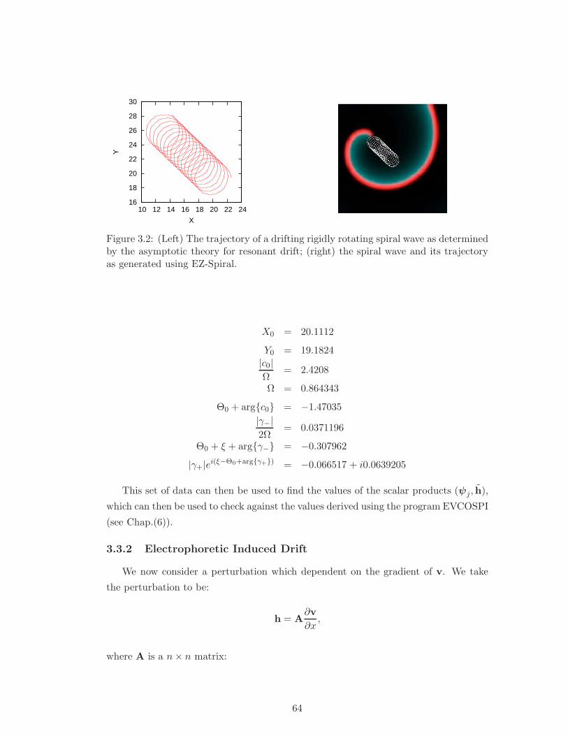
16
18
20
22
24
26
28
30
10 12 14 16 18 20 22 24
Y
X
Figure 3.2: (Left) The trajectory of a drifting rigidly rotating spiral wave as determinedby the asymptotic theory for resonant drift; (right) the spiral wave and its trajectoryas generated using EZ-Spiral.
X0 = 20.1112
Y0 = 19.1824
|c0|Ω
= 2.4208
Ω = 0.864343
Θ0 + argc0 = −1.47035
|γ−|2Ω
= 0.0371196
Θ0 + ξ + argγ− = −0.307962
|γ+|ei(ξ−Θ0+argγ+) = −0.066517 + i0.0639205
This set of data can then be used to find the values of the scalar products (ψj, h),
which can then be used to check against the values derived using the program EVCOSPI
(see Chap.(6)).
3.3.2 Electrophoretic Induced Drift
We now consider a perturbation which dependent on the gradient of v. We take
the perturbation to be:
h = A∂v
∂x,
where A is a n× n matrix:
64
A =
A1 0 · · 00 A2 0 · ·· 0 A3 0 ·· · · · 00 · · 0 An
.
We need to determine the transformed version of h. We know h is defined to be:
h = T(g−1)h(T(g)v0, r, t).
Firstly, we bear in mind how the transformation works. Given g ∈ SE(2), where
g = (R,Θ), then:
g :
(
xy
)
7→(
xy
)
=
(
XY
)
+
(
cos(Θ) − sin(Θ)sin(Θ) cos(Θ)
)(
xy
)
, (3.56)
g−1 :
(
xy
)
7→(
xy
)
=
(
cos(Θ) sin(Θ)− sin(Θ) cos(Θ)
)(
x−Xy − Y
)
. (3.57)
Next, we consider T(g)v0 (note that the transformations do not affect time depen-
dency; therefore, the dependence on time is omitted from now on):
T(g)v0(r) = v0(g−1r)
= v0(r)
= v0(r)
Therefore, we have:
ǫh(T (g)v0(r)) = ǫh(v0(r))
= A∂v0
∂x(r)
= A∂v0
∂x(r)
= A
(
∂v0
∂x(r)
∂x
∂x+
∂v0
∂y(r)
∂y
∂x
)
We now recall from Eqn.(3.57) expressions for x and y, hence:
ǫh(T (g)v0(r)) = A
(
∂v0
∂x(r)
∂x
∂x+
∂v0
∂y(r)
∂y
∂x
)
= A
(
cos(Θ)∂v0
∂x(r)− sin(Θ)
∂v0
∂y(r)
)
= v0(r)
= v0(x, y)
65
We now consider the action of the element g−1 on v0(x, y):
ǫT (g−1)h(T (g)v0(r)) = T (g−1)v0(r)
= v0(g(r))
= v0(X + x cos(Θ)− y sin(Θ),
Y + x sin(Θ) + y cos(Θ))
We now note that:
x = (x−X) cos(Θ) + (y − Y ) sin(Θ)
y = −(x−X) sin(Θ) + (y − Y ) cos(Θ)
Therefore, we have:
X + x cos(Θ)− y sin(Θ) = X + ((x−X) cos(Θ) + (y − Y ) sin(Θ)) cos(Θ)−(−(x−X) sin(Θ) + (y − Y ) cos(Θ)) sin(Θ)
= X + (x−X) cos2(Θ) + (y − Y ) sin(Θ) cos(Θ)
+(x−X) sin2(Θ)− (y − Y ) sin(Θ) cos(Θ)
= X + (x−X)(sin2(Θ) + cos2(Θ))
= x
Similarly, it can be shown that:
Y + x sin(Θ) + y cos(Θ) = y
Therefore, we have:
ǫh = v0(x, y)
= v0(r)
= A
(
cos(Θ)∂v0
∂x(r)− sin(Θ)
∂v0
∂y(r)
)
The equations of motion are now:
dR
dt= c0e
iΘ − eiΘ
[
2
(
ψ1,A
(
cos(Θ)∂v0
∂x(r)− sin(Θ)
∂v0
∂y(r)
))
+c0
ω0
(
ψ0,A
(
cos(Θ)∂v0
∂x(r)− sin(Θ)
∂v0
∂y(r)
))]
dΘ
dt= ω0 −
(
ψ0,A
(
cos(Θ)∂v0
∂x(r)− sin(Θ)
∂v0
∂y(r)
))
66
We now consider the inner products (ψi,A(cos(Θ)∂v0∂x
(r)− sin(Θ)∂v0∂y
(r))):
(ψi,A(cos(Θ)∂v0
∂x(r)− sin(Θ)
∂v0
∂y(r))) = cos(Θ)(ψi,A
∂v0
∂x(r))
− sin(Θ)(ψi,A∂v0
∂y(r))
= (ψi, ǫh)
We know from previous analysis that ∂xv0 and ∂yv0 can be expressed as a linear
combination of the eigenfunctions to the linear operator L.
∂xv0 =1
2(φ1 + φ1)
∂yv0 =1
2i(φ1 − φ1)
Therefore:
(ψi, ǫh) =cos(Θ)
2(ψi,A(φ1 + φ1))−
sin(Θ)
2i(ψi,A(φ1 − φ1))
=cos(Θ)
2(ψi,Aφ1) +
cos(Θ)
2(ψi,Aφ1)
−sin(Θ)
2i(ψi,Aφ1) +
sin(Θ)
2i(ψi,Aφ1)
We note that the choice of A is such that each element in the diagonal of A could
be non-zero and also they could all be different. The choice of these is arbitrary but
such that they are “small”. This therefore means that (ψi, Aφj) 6= δij . What we can
do is denote each of these scalar products using:
(ψi, Aφj) = Ai,j
Therefore:
(ψi, ǫh) =1
2Ai,1e
iΘ +1
2Ai,−1e
−iΘ
Therefore:
dR
dt= c0e
iΘ −(
c0
2ω0A0,1 + A−1,1
)
e2iΘ −(
c0
2ω0A0,−1 + A−1,−1
)
dΘ
dt= ω0 −
1
2(A0,1e
iΘ + A0,−1e−iΘ)
We will now integrate Eqns.(3.58) & (3.58) using asymptotic techniques, taking
advantage of the fact that Ai,j are small.
67
Firstly, we consider Eqn.(3.58) and note that A0,1 and A0,−1 are complex number,
and in fact we note that A0,1 = A0,−1.
We also assume that because A0,1 and A0,−1 are small, then:
A0,1 = ǫa0,1
A0,−1 = ǫa0,−1
Θ = Θ0 + ǫΘ1
Our problem now becomes:
dΘ0
dt+ ǫ
dΘ1
dt= ω0 −
ǫ
2(a0,1e
i(Θ0+ǫΘ1) + a0,−1e−i(Θ0+ǫΘ1)) + O(ǫ2)
⇒ dΘ0
dt+ ǫ
dΘ1
dt= ω0 −
ǫ
2(a0,1e
iΘ0 + a0,−1e−iΘ0) + O(ǫ2)
Splitting out the different orders in ǫ, we have:
ǫ0 :dΘ0
dt= ω0
ǫ1 :dΘ1
dt= −1
2(a0,1e
iΘ0 + a0,−1e−iΘ0)
We can see that (3.58) gives us:
Θ0 = ω0t + Θ0(0)
Substituting (3.3.2) into (3.58), we get:
dΘ1
dt= −1
2(a0,1e
i(ω0t+Θ0(0)) + a0,−1e−i(ω0t+Θ0(0)))
Θ1 = Θ1(0) +ia0,1
2ω0ei(ω0t+Θ0(0)) − ia0,−1
2ω0e−i(ω0t+Θ0(0))
Hence, our final expression for Θ is:
Θ = Θ(0) + ω0t + ǫ
(
ia0,1
2ω0ei(ω0t+Θ0(0)) − −ia0,−1
2ω0ei(ω0t+Θ0(0))
)
We now consider Eqn.(3.58). The first thing to note is that the coefficient to the
double angle exponential and also the constant term are just complex number, and in
fact these complex number have a small magnitude. Therefore, define the following
complex numbers:
ǫξ =c0
2ω0A0,−1 + A−1,−1
ǫζ =c0
2ω0A0,1 + A−1,1
68
Therefore, we get:
dR
dt= c0e
iΘ − ǫζe2iΘ − ǫξ + O(ǫ2) (3.58)
We also note that the initial conditions for Θ, say Θ(0) = Θ∗ give:
Θ = (ω0t + Θ∗) +iǫ
2ω0
(
a0,1ei(ω0t+Θ∗) − a0,−1e
−i(ω0t+Θ∗))
Now, consider eiΘ:
eiΘ = ei(ω0t+Θ∗) − ǫa0,−1
2ω0− ǫa0,1
2ω0e2i(ω0t+Θ∗) + O(ǫ2)
Similarly:
e2iΘ = e2i(ω0t+Θ∗) + O(ǫ)
Using these expression for the exponentials, Eqn.(3.58) now becomes:
dR
dt= c0e
i(ω0t+Θ∗) − ǫ
(
c0a0,1
2ω0+ ζ
)
e2i(ω0t+Θ∗)
+ǫ
(
c0a0,−1
2ω0− ξ
)
+ O(ǫ2)
⇒ dR
dt= c0e
i(ω0t+Θ∗) −(
c0
ω0A0,1 + A−1,−1
)
e2i(ω0t+Θ∗) + A−1,1 + O(ǫ2)
Hence, we can integrate to get:
R = R(0)− ic0
ω0ei(ω0t+Θ∗) +
i
2ω0
(
c0
ω0A0,1 + A−1,−1
)
e2i(ω0t+Θ∗)
−A−1,−1t + O(ǫ2)
⇒ R = R(0)− i|c0|ω0
ei(ω0t+Θ∗+argc0) +i
2ω0|A|e2i(ω0t+Θ∗+argA)
−|A−1,−1|eiargA−1,−1t + O(ǫ2)
where A =(
c0ω0
A0,1 + A−1,−1
)
Comparison with numerical simulations
As we did for resonant drift, we shall show an example of just how accurate our the-
ory is, by comparing the data from the numerical simulation (again using an amended
version of EZ-Spiral) with the analytical predictions.
69
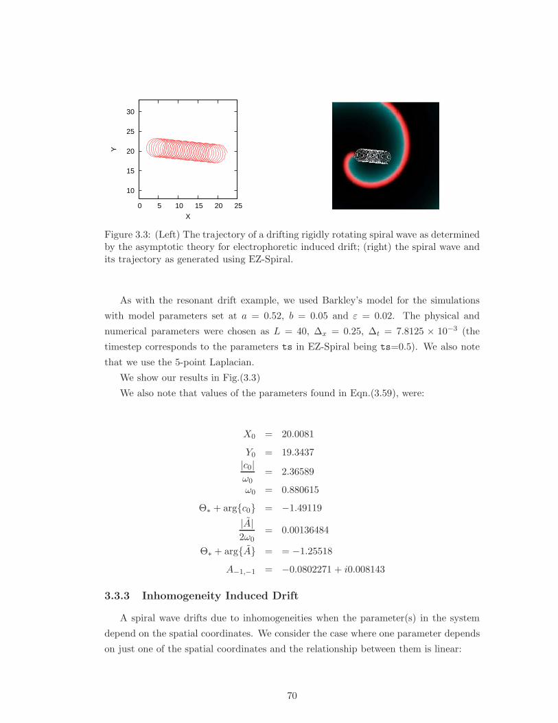
10
15
20
25
30
0 5 10 15 20 25
Y
X
Figure 3.3: (Left) The trajectory of a drifting rigidly rotating spiral wave as determinedby the asymptotic theory for electrophoretic induced drift; (right) the spiral wave andits trajectory as generated using EZ-Spiral.
As with the resonant drift example, we used Barkley’s model for the simulations
with model parameters set at a = 0.52, b = 0.05 and ε = 0.02. The physical and
numerical parameters were chosen as L = 40, ∆x = 0.25, ∆t = 7.8125 × 10⁻³ (the
timestep corresponds to the parameters ts in EZ-Spiral being ts=0.5). We also note
that we use the 5-point Laplacian.
We show our results in Fig.(3.3)
We also note that values of the parameters found in Eqn.(3.59), were:
X0 = 20.0081
Y0 = 19.3437
|c0|ω0
= 2.36589
ω0 = 0.880615
Θ∗ + argc0 = −1.49119
|A|2ω0
= 0.00136484
Θ∗ + argA = = −1.25518
A−1,−1 = −0.0802271 + i0.008143
3.3.3 Inhomogeneity Induced Drift
A spiral wave drifts due to inhomogeneities when the parameter(s) in the system
depend on the spatial coordinates. We consider the case where one parameter depends
on just one of the spatial coordinates and the relationship between them is linear:
70
α = α0 + α1x
where, for x = 0 we have α(0) = α0.
This leads to a symmetry breaking perturbation causing the wave to drift. We have
the following RDS:
∂u
∂t= D∇2u + f(u, α(x))
Expanding this using Taylor Series we get:
∂u
∂t= D∇2u + f(u, α0) + α1x
∂f
∂α(u, α0) + O(α2
1)
We see that the perturbation is now:
ǫh = α1x∂f
∂α(u, α0) + O(ǫ2)
where ǫ = α1 is gradient of the inhomogeneity and:
h = x∂f
∂α(u, α0)
We now have that h = h(v0, r) and we next need to calculate h. Firstly, consider:
h(T (g)v0, r) = h(T (g)v0(r), r)
= h(v0(g−1r), r)
= h(v0(r), r)
where r is given by:
(
xy
)
=
(
cos(Θ) sin(Θ)− sin(Θ) cos(Θ)
)(
x−Xy − Y
)
Therefore:
h(T (g)v0, r) = h(v0(r), r)
= x∂f
∂α(v0(r), α0)
= v(r)
71
Now, we apply the action of the inverse group element g−1 on h(T (g)v0, r):
h = T (g−1)h(T (g)v0, r)
= T (g−1)v(r)
= v(gr)
= v(X + x cos(Θ)− y sin(Θ), Y + x sin(Θ) + y cos(Θ))
= (X + x cos(Θ)− y sin(Θ))∂f
∂α(v0(r), α0)
The equations of motion are now:
dR
dt= c0e
iΘ − eiΘ
[
2
(
ψ1, (X + x cos(Θ)− y sin(Θ))∂f
∂α
)
− c0
ω0
(
ψ0, (X + x cos(Θ)− y sin(Θ))∂f
∂α
)]
,
dΘ
dt= ω0 −
(
ψ0, (X + x cos(Θ)− y sin(Θ))∂f
∂α
)
.
We now consider the inner products (ψi, (X + x cos(Θ)− y sin(Θ)) ∂f∂α
):(
ψi, (X + x cos(Θ)− y sin(Θ))∂f
∂α
)
= X
(
ψi,∂f
∂α
)
+ cos
(
Θ)(ψi, x∂f
∂α
)
− sin
(
Θ)(ψi, y∂f
∂α
)
Let us now define the following:
Ci,0 =
(
ψi,∂f
∂α
)
,
Ci,x =
(
ψi, x∂f
∂α
)
,
Ci,y =
(
ψi, y∂f
∂α
)
Hence, we have:
(
ψi, h)
= XCi,0 + cos Ci,x − sinCi,y
Therefore, we can write our equations of motion as follows. Firstly, dRdt
:
dR
dt= c0e
iΘ − α1eiΘ
(
X(2C−1,0 +c0
ω0C0,0) + cos(Θ)(2C−1,x +
c0
ω0C0,x)
− sin(Θ)(2C−1,y +c0
ω0C0,y)
)
72
Furthermore, if we define:
B0 = 2C−1,0 +c0
ω0C0,0,
2Bx = 2C−1,x +c0
ω0C0,x,
2iBy = 2C−1,y +c0
ω0C0,y,
then:
dR
dt= (c0 − α1XB0)eiΘ − α1(B
x −By)e2iΘ − α1(Bx + By).
Furthermore, if:
B+ = Bx + By,
B− = Bx −By.
then:
dR
dt= (c0 − α1XB0)eiΘ − α1B
−e2iΘ − α1B+.
Similarly we have that:
dΘ
dt= ω0 − α1(ψ0, (X + x cos(Θ)− y sin(Θ))
∂f
∂α)),
= ω0 − α1XC0,0 − α1 cos(Θ)C0,x + α1 sin(Θ)C0,y.
Finally, let us introduce further notation:
Ci,1 = (ψi, r∂f
∂α),
Ci,−1 = (ψi, r∂f
∂α),
where r = x + iy. It can be seen that:
Ci,x =1
2(Ci,1 + Ci,−1)
Ci,y =1
2i(Ci,1 − Ci,−1)
73
Therefore:
cos(Θ)C0,x − sin(Θ)C0,y =1
2(C0,1e
iΘ + C0,−1e−iΘ)
Hence:dΘ
dt= ω0 − α1XC0,0 −
α1C0,1
2eiΘ − α1C0,−1
2e−iΘ
Before we integrate the equations, we will firstly expand the solutions R and Θ in
orders of α1:
R = R0 + α1R1 + O(α21)
Θ = Θ0 + α1Θ1 + O(α21)
This leads to the equations:
dR0
dt= c0e
iΘ0 (3.59)
dR1
dt= ic0Θ1e
iΘ0 −X0B0eiΘ0 −B−e2iΘ0 −B+ (3.60)
dΘ0
dt= ω0 (3.61)
dΘ1
dt= −X0C0,0 −
C0,1
2eiΘ0 − C0,−1
2e−iΘ0 (3.62)
We will now integrate Eqns.(3.61), (3.59), (3.62) and (3.60), in that order.
Firstly, Eqn.(3.61) gives us, when integrated:
Θ0 = Θ∗ + ω0t
Next, we integrate Eqn.(3.59) to get:
R0 = R∗ −ic0
ω0ei(Θ∗+ω0t)
which gives us:
X0 = X∗ −i
2ω0
(
c0eiΘ0 − c0e
−iΘ0)
Next, we consider (3.62):
dΘ1
dt= −
(
X∗ −i
2ω0
(
c0eiΘ0 − c0e
−iΘ0)
)
C0,0 −C0,1
2eiΘ0 − C0,−12
e
−iΘ0
dΘ1
dt= −X∗C0,0 −
(
C0,1
2− ic0C0,0
2ω0
)
eiΘ0 −(
C0,−1
2+
ic0C0,0
2ω0
)
e−iΘ0
74
Integration gives:
Θ1 = Θ+ −X∗C0,0t + PeiΘ0 + P e−iΘ0
where:
P =i
2ω0
(
C0,1 −ic0C0,0
ω0
)
Before we move on to the final equation, we note that the perturbed part of Θ, i.e.
Θ1 must be bounded for our theory to work. This must mean that C0,0 = 0, otherwise
Θ1 is not bounded:
Θ1 = Θ+PeiΘ0 + P e−iΘ0
where P is no now given by:
P = − iC0,1
2ω0
Finally, we can consider Eqn.(3.60):
dR1
dt= ic0Θ1e
iΘ0 −X0B0eiΘ0 −B−e2iΘ0 + α1B
+
dR1
dt= (ic0 −X∗B
0)eiΘ0 +
(
ic0P +ic0B
0
2ω0−B−
)
e2iΘ0
+
(
ic0P −ic0B
0
2ω0+ B+
)
Integration gives:
R1 = R+ −i
ω0(ic0 −X∗B
0)eiΘ0 − i
2ω0
(
ic0P +ic0B
0
2ω0−B−
)
e2iΘ0
+
(
ic0P −ic0 + B+
2ω0−B−
)
t
R1 = R+ + A1eiΘ0 + A2e
2iΘ0 + A3t
where:
75
A1 = − i
ω0(ic0 −X∗B
0)
A2 = − i
2ω0
(
ic0P +ic0B
0
2ω0−B−
)
A3 = ic0P −ic0 + B+
2ω0−B−
We also note that the velocity of the drift, A3, can be expressed as:
A3 =ic0C−1,0
ω0+ C−1,−1
Therefore, the final full equations motion of the tip of a rigidly rotating spiral wave
which is drifting due to an inhomogeneity induced drift, are given by:
R(t) = R(0)− ic0
ω0ei(Θ∗+ω0t) + α1A1e
i(Θ∗+ω0t)
+α1A2e2i(Θ∗+ω0t) + α1A3t + O(α2
1)
Θ(t) = Θ(0) + ω0t + α1Pei(Θ∗+ω0t) + α1P e−i(Θ∗+ω0t) + O(α21)
3.4 Floquet Theory - Periodic Solutions
3.4.1 Introduction
In the next stage of our work, we consider the limit cycle solutions in the functional
space corresponding to spiral wavesolutions. Some authors denote this phenomenon as
Relative Periodic Solutions. In general, limit cycle solutions correspond to Meandering
Spiral Waves.
The stability of these limit cycles is of utmost importance. Unstable solution can
lead to multiple solutions, for instance, and also solutions with multiple tips and arms,
which are not covered by this theory. We consider only stable limit cycle solutions.
We saw in Sec.(3.2) that the equations of motion for a drifting rigidly rotating wave
were of the form:
dR
dt=
[
c0 − ǫ(2(ψ1, h(v0, r, t)) +c0
ω0(ψ0, h(v0, r, t)))
]
eiΘ
dΘ
dt= ω0 + ǫ(ψ0, h(v0, r, t))
where c0 and ω0 are constant and form the Euclidean Projection part of the quotient
76
solution. Therefore, since they are constant, we have an equilibrium in the quotient
space.
We now wish to consider non constant c0(t) and ω0(t). We therefore wish to study
the solutions in the quotient system to the Reaction-Diffusion-Advection system of
equations (3.22) in the functional space:
dV
dt= F(V) + (c[V], ∂r)V + ω[V]∂θV + ǫH(V, t)(V, t)
We now consider a general system of equations as shown below which will be dis-
cussed in the next section:
dV
dt= g(V) + ǫk(V, t)
where V, g, k ∈ Rn. The system (3.4.1) is a functional space analogue of (3.4.1)
3.4.2 General Floquet Theory
Firstly, consider system (3.4.1) with k = 0 with the following form:
dV
dt= g(V) (3.63)
We assume that the solutions to (3.63) are periodic and that they are perturbed
with the following form:
V(t) = V0(t) + ǫV1(t) (3.64)
We also assume that the unperturbed solution V0(t) is a known limit cycle solution
of period T :
V0(t + T ) = V0(t)
Substituting (3.64) into (3.63) and splitting out the orders of ǫ, we get:
ǫ0 :dV0
dt= g(V0)
ǫ1 :dV1
dt= G(t)V1 (3.65)
where G(t) = ∂g∂V
∣
∣
∣
V=V0(t)is a matrix of first order partial derivatives of g(V) evaluated
at V0(t).
77
Since we assume that we know the solution V0(t), we will consider for the remainder
of this section the solution V1(t), and its evolution as determined by Eqn.(3.65)
Consider G(t). This matrix of functions is periodic with period T since it is evalu-
ated at V0(t) which is periodic with period T :
G(t + T ) = G(t)
Now, any solution to Eqn.(3.65) can be expressed as a linear combination of n-
linearly independent solutions to (3.65), where the n-linearly independent solutions
form the columns of a matrix, Q(t), known as the Fundamental Matrix. Since any
solution to (3.65) can be expressed as a linear combination of linearly independent
solutions to (3.65), then any solution can be expressed as:
V1(t) = Q(t)C
where C is a constant vector and is equal to the initial value of V1(t), i.e.:
V1(t) = Q(t)V1(0)
Now, since the columns of Q(t) are independent solutions to (3.65), then Q(t) itself
must satisfy (3.65):
Q(t) = G(t)Q(t)
where the dot notation represents time derivatives. Now if Q(t) is a solution to (3.65)
then so too is Q(t + T ):
Q(t + T ) = G(t + T )Q(t + T )
Q(t + T ) = G(t)Q(t + T )
So, if Q(t) is a fundamental matrix, then so too is Q(t + T ).
Theorem 3.4.1. [35] Given a fundamental matrix Q(t), then Q(t + T ) is linearly
dependent on Q(t). Furthermore, if:
Q(t) = [qij(t)]
then we have that:
Q(t + T ) = [qij(t + T )] =
[
n∑
k=1
qik(t)bkj
]
= Q(t)B (3.66)
78
where bkj are constant and B is a constant matrix with B = [bkj].
Definition 3.4.2. The Monodromy Matrix, M is defined as the matrix Q evaluated
at an initial time, t0:
M = Q−1(t0)Q(t0 + T )
This implies that the constant matrix B above is actually equal to the Monodromy
Matrix. Also, we generally have that t0 = 0 and also that Q(0) = I, where I is an
identity matrix. Hence, the definition of the Monodromy Matrix reduces to:
M = Q(T )
An immediate consequence of this is that if we consider Eqn.(3.66):
Q(nT ) = Mn
Which implies that any solution evaluated at t = T is:
V1(nT ) = MnV1(0)
It follows that the stability of the solutions V1 to (3.65) is done by studying the
eigenvalues of M. These eigenvalues are called the Floquet Multipliers of the system
(3.65), and are given by:
det(M− µI) = 0, for µ = (µ1, · · · , µn) (3.67)
We note that if |µi| < 1 ∀i = 1, . . . , n then the system is stable. Else, if ∃µi > 1
for some i, then the system is unstable. There always exists one multiplier µ∗ = 1.
The reason for this is that we require periodic solutions, and if there does not exist
a multiplier equal to one, then we will not get periodic solutions. We shall show a
proof of this in Sec.(3.4.8). This will become more evident when we state Thm.(3.4.4).
We assume that we are dealing with stable solutions and therefore we must have that
|µi| < 1 ∀i = 1, . . . , n and i 6= ∗.Furthermore, we come to the following definition:
Definition 3.4.3. Let µ be the Floquet Multipliers as defined by (3.67) corresponding
to the period T of G(t). Then, the corresponding Floquet Exponent, ρ, is defined as:
eρT = µ.
We now come to the following fundamental theorem:
79
Theorem 3.4.4. [35] Suppose that M has n distinct multipliers, µi for i = 1, .., n.
Then Eqn.(3.65) has n linearly independent solutions of the form:
qi(t) = pi(t)eρit
where the pi(t) are functions with period T . The qi(t) are the columns of the Funda-
mental Matrix which therefore has the following form:
Q(t) = P(t)eRt
where R is a constant matrix, known as the Indicator Matrix.
From this Theorem, it immediately follows that at t = 0 we have:
I = P(0)
and also at time t = T , we get:
Q(T ) = eRT
due to the T -periodicity of P(t). We know that the Monodromy Matrix, M, is the
Fundamental Matrix evaluated at time t = T , and so we come to another important
derivation:
M = eRT
Now, any solution to Eqn.(3.65) can be therefore be expressed as:
V1i(t) = Q(t)C = P(t)eRtV1(0) =∑
i
pi(t)eρitV1i(0)
where V1(t) = (V11(t), V12(t), . . . , V1n(t)).
So, at time T , we have:
V1(T ) = P(T )eRTV1(0) = P(0)eRTV1(0) = MV1(0)
with the second equation coming from the periodicity of P . So, generally, for time nT ,
we have:
80
V1(nT ) = MnV1(0) (3.68)
To complete the picture, let us consider the solution at time t = t + T :
V1(t + T ) = Q(t + T )V1(0) = Q(t)Q(T )V1(0) = Q(t)MV1(0)
Now, let us introduce the multiplier problem for M:
(M− µI)β = 0
where β is the eigenvector corresponding to the the Floquet multiplier of M.
Generally, there is a solution V1, called the eigensolution, which is a linear com-
bination of the columns of the Fundamental Matrix, such that V1(0) = β:
V1(t) = Q(t)β
Therefore:
V1(t + T ) = Q(t)Mβ = Q(t)µβ = µQ(t)β = µV1(t)
So, in general it can be shown that:
V1(t + nT ) = µnV1(t)
Let us now claim the following. We know that the eigenvalues to R are ρ and
satisfy:
det(R− ρiI) = 0
The eigenvalue problem is:
Rαi = ρiαi
where αi is an eigenvector of R. This therefore means that:
eRtαi = eρitαi (3.69)
81
Then there will exist a solution to (3.65) of the form:
V1i(t) = Q(t)αi = P(t)eRtαi = P(t)eρitαi = eρitP(t)αi = eρitφi(t)
where φi(t) is periodic and defined as the Eigenfunction corresponding to the Floquet
Exponent, ρi. We shall call this eigenfunction the Floquet Eigenfunction:
φi(t) = P(t)αi
Let us now derive the eigenvalue problem relating to these eigenfunctions. From
Eqn.(3.69) we have:
eRtαi = eρitαi
PeRtαi = eρitPαi
PeRtP−1Pαi = eρitPαi
PeRtP−1φi = eρitφi
QP−1φi = eρitφi
Therefore, we have an operator defined as QP−1 for which the above equation holds
true.
Let us now consider the solution V1i(t) = eρitφi(t),and substitute this into Eqn.(3.65):
ρieρitφi(t) + eρitφi(t) = G(t)eρitφi(t)
⇒ ρiφi(t) + φi(t) = G(t)φi(t)
⇒ φi(t) = (G(t)− ρiI)φi(t)
3.4.3 Floquet Eigenfunctions corresponding to Meander
We will now consider the unperturbed Reaction-Diffusion-Advection system of equa-
tions, whose solution is now a meandering spiral wave. This time, let us consider the
system in our original space:
∂v0
∂t= D∇2v0 + f(v0) + (c(v0),∇)v0 + ω(v0)∂θv0 (3.70)
Let us now differentiate Eqn.(3.70) with respect to x:
82
∂
∂x
(
∂v0
∂t
)
= D∇2
(
∂v0
∂x
)
+∂f(v0)
∂v0
(
∂v0
∂x
)
+ cx(v0)∂2v0
∂x2+ cy(v0)
∂2v0
∂x∂y
+ω(v0)∂
∂x
(
x∂v0
∂y− y
∂v0
∂x
)
+ O(ǫ2)
∂
∂t
(
∂v0
∂x
)
= D∇2
(
∂v0
∂x
)
+ f′(v0)
(
∂v0
∂x
)
+ cx(v0)∂
∂x
(
∂v0
∂x
)
+ cy(v0)∂
∂y
(
∂v0
∂x
)
+ω(v0)∂v0
∂y+ ω(v0)
(
x∂
∂y
∂v0
∂x− y
∂
∂x
∂v0
∂x
)
+ O(ǫ2)
∂
∂t
(
∂v0
∂x
)
= D∇2
(
∂v0
∂x
)
+ f′(v0)
(
∂v0
∂x
)
+ (c(v0),∇)
(
∂v0
∂x
)
+ ω(v0)∂
∂θ
(
∂v0
∂x
)
+ω(v0)
(
∂v0
∂y
)
+ O(ǫ2)
∂
∂t
(
∂v0
∂x
)
= G(t)
(
∂v0
∂x
)
+ ω(v0)
(
∂v0
∂y
)
+ O(ǫ2)
where G(t) is given by:
G(t)α = D∇2α + f′(v0)α + (c(v0),∇)α + ω(v0)∂α
∂θ(3.71)
Similarly, by differentiating Eqn.(3.70) with respect to y, we get:
∂
∂t
(
∂v0
∂y
)
= G(t)
(
∂v0
∂y
)
− ω(v0)
(
∂v0
∂x
)
+ O(ǫ2) (3.72)
We see that if we consider (3.71)+i(3.72), then:
∂
∂t
(
∂v0
∂x+ i
∂v0
∂y
)
= G(t)
(
∂v0
∂x+ i
∂v0
∂y
)
− iω(v0)
(
∂v0
∂x+ i
∂v0
∂y
)
+ O(ǫ2)
(
G(t)− ∂
∂t
)
φ1 = iω(v0)φ1
where φ1 is the eigenfunction in a comoving frame of reference given by:
φ1 =∂v0
∂x+ i
∂v0
∂y
and therefore the eigenfunction in the laboratory frame of reference needs to be trans-
formed:
φ1 = eiΘ0φ1 (3.73)
83
where Θ0 satisfies:
Θ0 = ω(v0)
Differentiating Eqn.(3.73) with respect to t, we get:
∂φ1
∂t= iΘ0e
iΘ0φ1 + eiΘ0∂φ1
∂t∂φ1
∂t= iω(v0)e
iΘ0φ1 + eiΘ0G(t)φ1 − iω(v0)eiΘ0φ1
∂φ1
∂t= eiΘ0G(t)φ1
∂φ1
∂t= G(t)φ1
(
G(t)− ∂
∂t
)
φ1 = 0
This is equivalent to the Floquet exponent problem given by:
(
G(t)− ∂
∂t
)
φi = ρiφi
Hence, the eigenfunction φ1 corresponds to the zero Floquet exponent. Similarly,
it can be shown that the complex conjugate of φ1 = φ−1 is given by,
φ−1 = e−iΘ0φ−1
where,
φ−1 =∂v0
∂x− i
∂v0
∂y
and satisfies:
(
G(t)− ∂
∂t
)
φ−1 = 0
Again, we see that φ−1 corresponds to the zero Floquet exponent.
Finally, let us consider differentiating Eqn.(3.70) with respect to θ. After some
analysis, we get:
∂
∂t
(
∂v0
∂θ
)
= G(t)
(
∂v0
∂θ
)
− cx(v0)
(
∂v0
∂y
)
+ cy(v0)
(
∂v0
∂x
)
+ O(ǫ2)
Let us define the eigenfunction φ0 as:
84
φ0 =∂v0
∂θ+ αφ1 + βφ−1
Now, consider the operation of G(t) on φ0:
G(t)φ0 = G(t)∂v0
∂θ+ αG(t)φ1 + βG(t)φ−1
G(t)φ0 =∂
∂t
(
∂v0
∂θ
)
+ cx(v0)
(
∂v0
∂y
)
− cy(v0)
(
∂v0
∂x
)
+α
(
iω(v0)φ1 +∂
∂tφ1
)
+ β
(
−iω(v0)φ−1 +∂
∂tφ−1
)
G(t)φ0 =∂
∂t
(
∂v0
∂θ
)
+cx(v0)
2i
(
φ1 − φ−1
)
− cy(v0)
2
(
φ1 + φ−1
)
+α
(
iω(v0)φ1 +∂
∂tφ1
)
+ β
(
−iω(v0)φ−1 +∂
∂tφ−1
)
G(t)φ0 =∂
∂t
(
∂v0
∂θ+ αφ1 + βφ−1
)
+ φ1
(
cx(v0)
2i− cy(v0)
2+ αiω(v0)
)
−φ−1
(
cx(v0)
2i+
cy(v0)
2+ βiω(v0)
)
G(t)φ0 =∂
∂tφ0 + φ1
(
− ic(v0)
2+ αiω(v0)
)
− φ−1
(
− ic(v0)
2+ βiω(v0)
)
So, if:
α =c(v0)
2ω(v0)
β =c(v0)
2ω(v0)
then we have:
φ0 =∂v0
∂θ+
c(v0)
2ω(v0)φ1 +
c(v0)
2ω(v0)φ−1
⇒ φ0 =∂v0
∂θ+
c(v0)
2ω(v0)φ1e
−iΘ0 +c(v0)
2ω(v0)φ−1e
iΘ0
which in turn implies that:
G(t)φ0 =∂
∂tφ0
(
G(t)− ∂
∂t
)
φ0 = 0
85
Clearly, we have that:
φ0 = φ0
and φ0 satisfies:
(
G(t)− ∂
∂t
)
φ0 = 0
implying that φ0 is another eigenfunction of the Floquet exponent problem for the
zero exponent.
To summarise, we have in the laboratory frame of reference:
φ∗ = ∂v0∂τ
, ρ∗ = 0
φ1 = eiΘ0
(
∂v0∂x
+ i∂v0∂y
)
, ρ1 = 0
φ−1 = e−iΘ0
(
∂v0∂x− i∂v0
∂y
)
, ρ−1 = 0
φ0 = ∂v0∂θ
+ c(v0)2ω(v0)φ1e
−iΘ0 + c(v0)2ω(v0)
φ−1eiΘ0 , λ0 = 0
(3.74)
In the comoving frame of reference, we have:
φ∗ = ∂v0∂τ
, ρ∗ = 0
φ1 = ∂v0∂x
+ i∂v0∂y
, ρ1 = iω(v0)
φ−1 = ∂v0∂x− i∂v0
∂y, ρ−1 = −iω(v0)
φ0 = ∂v0∂θ
+ c(v0)2ω(v0)φ1 + c(v0)
2ω(v0)φ−1 , ρ0 = 0
(3.75)
3.4.4 Floquet Theory: The Adjoint Problem
We summarize several results from the previous section. Firstly, we note that for
the system V1 = G(t)V1, we have the Fundamental Matrix defined as:
Q(t) = P(t)eRt
where R is a constant matrix known as the Indicator Matrix and P(t+T ) = P(t). The
eigenvalues, ρi, to R are known as the Floquet Exponents and satisfy:
Rαi = ρiαi
where αi are the corresponding eigenvectors. Also, the Fundamental Matrix evaluated
at T , where T is the period of the solution to the system, is known as the Monodromy
Matrix, M, whose eigenvalues are the Floquet Multipliers.
86
Now, Q(t) consists of n independent fundamental solutions, qi, which are defined
as:
qi(t) = pi(t)eρit = Q(t)αi (3.76)
We then defined the Floquet Eigenfunctions as:
φi(t) = P(t)αi
which satisfy:
(
G(t)− d
dt
)
φi = ρiφi ⇒ Lφi = ρiφi
where:
Lα = G(t)α− dα
dt
We can now define the adjoint problem. The adjoint system of equation to V1 =
G(t)V1 is given by:
⇒ dW
dt= −G+(t)W (3.77)
The eigenfunction generated by this system are ψj , which are periodic and satisfy:
(
G+(t) +d
dt
)
ψj = σjψj
Also they take the following form:
ψj(t) = P(t)βj
Using:
L+β = G+(t)β +dβ
dt
our adjoint eigenproblem is :
L+ψj = σjψj
The eigenfunctions, ψj, are called the Floquet response functions.
87

3.4.5 Biorthogonality Conditions
There exists a biorthogonality condition between the Floquet response functions,
ψj, and the eigenfunctions, φi, to the linear operator L. Let us define the scalar product
between these in two different ways:
(1) (ψj,φi) = 〈ψj,φi〉 (3.78)
(2) (ψj,φi) =
∫ T2
−T2
〈ψj(τ),φi(τ)〉dτ (3.79)
where definition (1) is local in time, with definition (2) being averaged over the period
of the spiral, i.e. global in time, and 〈αi,βj〉 is the usual Hermitian scalar product.
The first definition means that the biorthogonality condition takes the form of the
scalar product of the two functions in question for any given time.
It would be beneficial for us if we could use definition (1) due to the fact that we
would not have to integrate nor would we have to consider a range of times, but just
one particular moment.
Let us consider definition Eqn.(3.78) and define the following:
< ψj ,φi >= gji(t) (3.80)
Let us now differentiate (3.80):
dgji
dt= < ψj ,φi > + < ψj , φi >
Using the following:
φi = (G(t)− ρi)φi
ψj = −(G(t)+ − σj)ψj
88
we get:
dgji
dt= 〈−G(t)+ψj ,φi〉+ 〈σjψj,φi〉
+〈ψj,G(t)φi〉 − 〈ψj , ρiφi〉dgji
dt= −〈ψj,G(t)φi〉+ σj〈ψj,φi〉
+ < ψj,G(t)φi〉 − ρi〈ψj ,φi〉dgji
dt= σj〈ψj ,φi〉 − ρi〈ψj,φi〉
dgji
dt= (σj − ρi)〈ψj ,φi〉
dgji
dt= (σj − ρi)gji
Since L+ is an adjoint operator to L with respect to the global scalar product, we
have:for i = j ρj = σj
for i 6= j 〈ψj,φi〉 = 0
Going back to our differential equation in gji, we have:
dgji
dt= (σj − ρi)gji
⇒ gji(t) = gji(0)e(σj−ρi)t
So, if i = j:
gii(t) = gii(0)
We know biorthogonality means that:
(ψj ,φi) =
∫ T2
−T2
gij(τ)dτ = δji
This therefore implies that:
〈ψj ,φi〉 =δji
T
3.4.6 Solvability Conditions
Now, we have that φi and ψj satisfy:
Lφi = ρiφi
L+ψj = ρjψj
89
Let us consider the fundamental matrix of (3.77). We assume that it takes the
following form:
Q(t) = PeRt
So, Q(t) also satisfies (3.77) and gives:
dQ
dt= G+(t)Q
Now, we know that the eigenvalues to R are σj = ρj . So let us assume that the
eigenvectors are β and satisfy;
Rβj = ρjβj
Now if the eigenfunctions are orthogonal, then the eigenvectors must also be or-
thogonal:
(βj ,αi) = δji (3.81)
So, if we substitute the definitions of φi and ψj into (ψj,φi) = δji and use (3.81),
then we get:
ψj(t) = (P−1)+(t)βj
Therefore, we now have a complete algorithm to find the Floquet response functions.
We now need to define, a suitable solvability condition. In order to have a unique
solution for V1, let us impose the following orthogonality condition:
(ψ∗,V1) = 0
where ψ∗ is the the adjoint floquet eigenfunction to the adjoint linear operator L+
corresponding to the unit multiplier, i.e. µ∗ = 1 ⇒ ρ∗ = 0.
Let us differentiate (ψ∗,V1) with respect to time:
d
dt(ψ∗,V1) = 0
(ψ∗, V1) + (ψ0,V1) = 0
⇒ (ψ∗, V1) = −(ψ0,V1)
Using Eqn.(3.4.4), we have:
90
(ψ∗, V1) = −(−G(t)+ψ∗ + σ∗ψ∗,V1)
⇒ (ψ∗, V1) = (G(t)+ψ∗,V1)
⇒ (ψ∗, V1) = (ψ∗,G(t)V1)
Hence, we now have two solvability conditions:
(ψ∗,V1) = 0
(ψ∗, V1) = (ψ∗,G(t)V1)
3.4.7 Stability in a Perturbed System; Regular Perturbation Tech-niques.
We now consider the following perturbed system:
dV
dt= g(V) + ǫk(V, t) (3.82)
Like the unperturbed case (3.63), we assume that V has the regular form (3.64):
V(t) = V0(t) + ǫV1(t) + O(ǫ2) (3.83)
Substituting Eqn.(3.83) into (3.82), using Taylor expansion and splitting out into
orders of ǫ, we get:
ǫ0 :dV0
dt= g(V0) (3.84)
ǫ1 :dV1
dt= G(t)V1 + k(V0, t) (3.85)
As before, we assume that V0 is a limit cycle solution. Therefore, we concentrate
our efforts on (3.85). Furthermore, we see that, as before, G(t) is a periodic function
of period T and also we now have that k(V0, t) must be a periodic function also of
period T .
Since we know the solution to (3.84), we shall concentrate on the solutions to (3.85).
Firstly, we recall that G(t) is a matrix of partial derivatives of g(V):
G(t) =
[
∂gi
∂Vj
]
We also see that G(t) is periodic with period T . We therefore want to solve the
following ODE:
91
dV1
dt−G(t)V1 = k(t)
We do this by firstly considering the homogeneous equation to find a Complemen-
tary Function, and then use a suitable ansatz for the Particular Integral, which will
enable us to find the General Solution:
V1 = V1,CF + V1,P I
So, for the complimentary function, consider the homogeneous equation:
dV1,CF
dt= G(t)V1,CF (3.86)
We know from Floquet Theory that this has the solution:
V1,CF = Q(t)V1(0)
where we have an explicit expression for the Fundamental Matrix Q(t):
Q(t) = eR
G(t)dt
For a particular integral, we use the Method of Variation of Parameters [50]:
V1,P I = Q(t)A(t) (3.87)
This time, we assume that the vector premultiplied by Q(t) is time dependent.
Substituting (3.87) into (3.86) we get:
A(t) =
∫ t
0Q−1(η)k(η)dη
Therefore, the Particular Integral is :
V1,P I = Q(t)
∫ t
0Q−1(η)k(η)dη
giving the full solution to be:
V = V0(t) + ǫQ(t)
(
V1(0) +
∫ t
0Q−1(η)k(η)dη
)
+ O(ǫ2) (3.88)
A property that we require from the solutions V is that they are bounded. Numer-
ical results show that for large time periods (Chap.5), the spiral wave solution in the
92
quotient system remains bounded. The purpose of this part of the work is to analyt-
ically study the evolution of the limit cycles that are evident in the quotient system.
Therefore, we require that the limit cycle solutions remain bounded.
Let us show that, in general, the solution shown in (3.88) is NOT in fact bounded.
Consider the first order of ǫ part of (3.88) and let us assume that the vector function
k(t) can be expressed as:
k(t) =∑
i
ki(t)φi(t)
Therefore, the first order part of (3.88) now becomes:
V1(t) = Q(t)V1(0) +∑
i
Q(t)
∫ t
0Q−1(η)ki(η)φi(η)dη
Now, we know that φi(t) = P(t)αi, so therefore:
V1(t) = Q(t)V1(0) +∑
i
Q(t)
∫ t
0Q−1(η)ki(η)P(η)αidη
= Q(t)V1(0) +∑
i
Q(t)
∫ t
0ki(η)e−RηP−1(η)P(η)αidη
= Q(t)V1(0) +∑
i
Q(t)
∫ t
0ki(η)e−Rηαidη
= Q(t)V1(0) +∑
i
Q(t)
∫ t
0ki(η)e−ρiηαidη
= Q(t)V1(0) +∑
i
Q(t)αi
∫ t
0ki(η)e−ρiηdη
Now we know that αi are eigenvectors and that Q(t)αi = qi(t) = pi(t)eρit from
(3.76):
V1(t) = Q(t)V1(0) +∑
i
pi(t)eρit
∫ t
0ki(η)e−ρiηdη
= Q(t)V1(0) +∑
i
pi(t)
∫ t
0ki(η)e−ρi(η−t)dη
Now, we require that the elements ki of the perturbation are bounded. Also, we
note that t ≥ η and since we require stable limit cycles (meaning that ρi ≤ 0) then
e−ρi(η−t) ≪ 1, and using the fact that ρ0 = 0 and ρi6=0 < 0:
V1(t) = Q(t)V1(0) +∑
i6=0
pi(t)
∫ t
0ki(η)e−ρi(η−t)dη + p0(t)
∫ t
0k0(η)dη
⇒ V1(t) ≈ Q(t)V1(0) + p0(t)
∫ t
0k0(η)dη
93
for large time. Therefore we see that there will be a linear growth in V1(t) as time grows
and hence V1(t) is not bounded, unless of course if∫ t
0 k0(η)dη converges. Therefore, if∫ t
0 k0(η)dη does not converge, a singular perturbation technique is required.
3.4.8 Stability in an Perturbed System; Singular Perturbation Tech-niques.
Given the following system:
dV
dt= g(V) + ǫk(V) (3.89)
we assume a solution to (3.89) takes the following form:
V(t) = V0(t + θ(t)) + ǫV1(t + θ(t))
where θ(t) is a shift to time and can be thought of as a perturbation of the limit cycle’s
phase. Using the method of Strained Coordinates [50], let us introduce the following
notation:
τ = t + θ(t)
This means that our solution can be expressed as:
V(t) = V0(τ) + ǫV1(τ) (3.90)
Substituting (3.90) into (3.89) we get:
(1 + θ)dV0
dτ+ ǫ(1 + θ)
dV1
dτ= g(V0) + ǫG(τ)V1 + ǫk(V0)
where G(τ) = ∂g∂V
∣
∣
∣
V=V0
.
Splitting out the unperturbed and perturbed parts, we obtain:
UnperturbeddV0
dτ= g(V0)
Perturbed θdV0
dτ+ ǫ(1 + θ)
dV1
dτ= ǫG(τ)V1 + ǫk(V0)
This therefore means that θ must be of the order of epsilon, θ = O(ǫ). Let θ take
the following form:
94
θ = ǫA (3.91)
Before moving on to find an expression for A, we note that:
dθ
dt=
dθ
dτ
dτ
dtdθ
dt=
dθ
dτ(1 + θ)
dθ
dt=
dθ
dτ
1
1− dθdτ
dθ
dt=
dθ
dτ+ O(ǫ2)
Now, on substituting (3.91) into (3.91) and bearing in mind that ǫθV′1 = O(ǫ2), we
get:
AdV0
dτ+
dV1
dτ= G(τ)V1 + k(V0) + O(ǫ)
If S = k(V0)−AV′0, then we get:
dV1
dτ= G(τ)V1 + S + O(ǫ)
Consider this equation and premultiply it with the Floquet response functions cor-
responding to the unit multiplier:
(
ψj ,dV1
dτ
)
=(
ψj,G(τ)V1
)
+(
ψj,S)
−(
ψj ,V1
)
=(
ψj,G(τ)V1
)
+(
ψj,S)
(
G+ψj ,V1
)
=(
ψj,G(τ)V1
)
+(
ψj,S)
(
ψj ,G(τ)V1
)
=(
ψj,G(τ)V1
)
+(
ψj,S)
(
ψj ,S)
= 0 (3.92)
for j = ∗, 0,±1.
We now have the following relation:
95
(ψ∗,S) = 0
⇒ (ψ∗,k(V0)−AV′0) = 0
⇒ (ψ∗,k(V0))− (ψ∗, AV′0) = 0
⇒ (ψ∗,k(V0)) = (ψ∗, AV′0)
⇒ A(ψ∗,V′0) = (ψ∗,k(V0))
⇒ A(ψ∗,φ∗) = (ψ∗,k(V0))
⇒ A = (ψ∗,k(V0))
So the full closed system of equations which governs the dynamics of the perturbed
limit cycle is:
dV0
dτ= g(V0)
dV1
dτ= G(τ)V1 + S + O(ǫ) (3.93)
dθ
dτ= ǫ(ψ∗,k(V0))
where S = k(V0)−(ψ∗,k)V′0. Now, we note that Eqn.(3.93) is equivalent to Eqn.(3.85),
and therefore we will perform a similar exercise to see if V1 is now bounded.
Firstly, we note that the solution to (3.93) can be split out as the sum of a comple-
mentary function and a particular integral.
V1 = V1,CF + V1,P I
The complementary function is:
V1,CF = Q(τ)V1(0)
and the particular integral turns out to be:
V1,P I = Q(τ)
∫ τ
0Q−1(t)S(t)dt
Therefore, the full solution is:
V(τ) = V0(τ) + ǫQ(τ)V1(0) + ǫQ(τ)
∫ τ
0Q−1(t)S(t)dt (3.94)
96
We now show that, in general, the solution shown in (3.94) is bounded. Consider
the first order of ǫ part of (3.94) and let us assume that the vector function S(t) can
be expanded in its eigenbasis as:
S(t) =∑
i
si(t)φi(t)
It follows that:
S(τ) =∑
i
si(τ)φi(τ)
⇒ (ψi,S(τ)) = si(τ)
⇒ si(τ) = (ψi,k− (ψ∗,k)V′0)
⇒ si(τ) = (ψi,k)− (ψ∗,k)(ψi,V′0)
⇒ si(τ) = (ψi,k)− (ψ∗,k)(ψi,φ∗)
⇒ si(τ) = (ψi,k)− (ψ∗,k)δi,∗
Using a technique similar to that used in Sec.(3.4.7), we find that:
V1(τ) = Q(τ)V1(0) +∑
i
pi(τ)
∫ τ
0si(t)e
−ρi(t−τ)dt (3.95)
Consider the right hand side of Eqn.(3.95). We know that Q(τ) is periodic and
hence bounded. Therefore, since V1(0) is a constant vector, then Q(τ)V1(0) is a
vector whose components are all bounded. The second term on the right hand side is
also bounded which is seem by taking the absolute value of the integral and using the
Absolute Value Integral Inequality :
∣
∣
∣
∣
∣
∑
i
pi(τ)
∫ τ
0si(t)e
−ρi(t−τ)dt
∣
∣
∣
∣
∣
≤∑
i
|pi(τ)|∣
∣
∣
∣
∫ τ
0si(t)e
−ρi(t−τ)dt
∣
∣
∣
∣
≤∑
i
|pi(τ)|∫ τ
0
∣
∣
∣si(t)e−ρi(t−τ)
∣
∣
∣dt
≤∑
i
|pi(τ)|∫ τ
0|si(t)| e−ρi(t−τ)dt
Now, we know that pi(τ) are periodic and hence bounded by, say, pi, and also if
we assume that the perturbation k is bounded then we also have that si(τ) are also
bounded:
||k(τ)|| ≤ K ⇒ |si(τ)| < ci
97
for some K and ci. Therefore, we have:
∣
∣
∣
∣
∣
∑
i
pi(τ)
∫ τ
0si(t)e
−ρi(t−τ)dt
∣
∣
∣
∣
∣
<∑
i
pi
∫ τ
0cie
−ρi(t−τ)dt
<∑
i
pici
∫ τ
0e−ρi(t−τ)dt
<∑
i
pici
[
− 1
ρie−ρi(t−τ)
]τ
0
<∑
i
pici
ρi(1− eρiτ )
We note that ρi ≤ 0. Therefore,we have:
∣
∣
∣
∣
∣
∑
i
pi(τ)
∫ τ
0si(t)e
−ρi(t−τ)dt
∣
∣
∣
∣
∣
<∑
i
pici
ρi
which shows that provided the sum on the right hand side above converges, we have
that V1 is bounded.
3.5 Application to the Quotient System
We will now apply the theory reviewed and developed in Sec.(3.4) to our own
particular problem, which is the study of meandering spiral waves that are the subject
of symmetry breaking perturbations. We know from [9, 16, 64, 28] that in a suitable
functional space, we have limit cycle solutions. Therefore, we will now apply Floquet
Theory techniques to this specific problem.
3.5.1 Application to the Quotient System
In a suitable functional space, which we can think of as the space of group orbits,
we saw that we have the following equations, the solutions to which are spiral waves in
a frame of reference comoving with the tip of the spiral wave.
dV
dt= F(V) + (c, ∂r)V + ω∂θV + ǫH(V, t)
V (1)(t) = u∗ (3.96)
V (2)(t) = v∗ (3.97)
∂xV (1) = 0 (3.98)
98
We note that we can reformulate this system of equations by resolving (3.96)-(3.98)
with respect to c and ω, so that c and ω depend on V:
dV
dt= F(V) + (c(V), ∂r)V + ω(V)∂θV + ǫH(V, t) (3.99)
We will use (3.99) for the remainder of this theory.
In Sec.(3.4) we took a general equation of the form:
dV
dt= g(V) + ǫk(V, t)
and we saw that we needed to consider shifts in time and a new time variable was
introduced:
τ = t + θ(t)
which can be written as:
t = τ − θ(τ)
We also note that we can expand our solutions in powers of ǫ as follows:
V(τ) = V0(τ) + ǫV1(τ) + O(ǫ)
c(τ) = c0(τ) + ǫc1(τ) + O(ǫ)
ω(τ) = ω0(τ) + ǫω1(τ) + O(ǫ)
where c0, c1, ω0 and ω1 are given by:
c0(τ) = c(V0)
c1(τ) =dc(V0)
dVV1
ω0(τ) = ω(V0)
ω1(τ) =dω(V0)
dVV1
We therefore find that we get the following system of equations:
99
dV0
dτ= g(V0)
dV1
dτ= LV1 + S + O(ǫ)
dθ
dτ= ǫ(ψ∗,k)
where
g(V0) = F(V0) + (c0, ∂r)V0 + ω0∂θV0
LV1 =dF(V0)
dV+ (c0, ∂r)V1 + ω0∂θV1
S = (c1, ∂r)V0 + ω1∂θV0 + H(V, t)− (ψ0, H)dV0
dτ(3.100)
Finally, in order to make V1 a unique solution, we require an additional condition
which guarantees uniqueness. We choose this to be:
(ψ∗,V1) = 0
An immediate consequence of this condition is the solvability condition (3.92).
3.5.2 Full Equations of Motion
Let us take the scalar product of (3.100) with ψi:
(ψi,S) = c1x(ψi, ∂xV0) + c1y(ψi, ∂yV0)
+ω1(ψi, ∂θV0) + (ψi, H(V, t))− (ψ∗, H)(ψi,dV0
dτ) (3.101)
Using the expressions for the eigenfunctions φi in the comoving frame of reference,
(3.75), the solvability condition (3.92)and also also Eqn.(3.101), we have:
i = 0 : ω1 = −(ψ0, H(V, t)) (3.102)
i = 1 :c1
2− ω1c0
2ω0= −(ψ1, H(V, t))
i = −1 :c1
2− ω1c0
2ω0= −(ψ−1, H(V, t))
⇒ c1 =ω1c0
ω0− 2(ψ−1, H(V, t)) (3.103)
Therefore, our full equations of motion are:
dR
dt=
[
c0(t)− ǫc0(t)
ω0(t)(ψ0(t + θ(t)), H(V, t))− 2ǫ(ψ−1(t + θ(t)), H(V, t))
]
eiΘ + O(ǫ2)
dΘ
dt= ω0(t)− ǫ(ψ0(t + θ(t)), H(V, t)) + O(ǫ2)
dθ
dt= ǫ(ψ∗(t + θ(t)), H(V, t)) + O(ǫ2)
100
where V = V(τ) = V(t + θ(t)), and ψj = ψj(τ) = ψj(t + θ(t)).
We note that if the amplitude of meander vanishes, then these equations are similar
to the equations for the rigidly rotating spiral wave without meander. This is as
expected. However, the difference in this instance is that the velocities c0 and ω0, and
also the response functions, are no longer constant but are dependent on time. The
theory so far developed in this thesis can equally apply to rigidly rotating spiral waves
and also meandering spiral, both of which are subject to drift.
However, we cannot say the same about the theories developed by Keener and also
Biktashev. They were developed specifically for rigidly rotating spiral waves. No peri-
odic solutions were assumed in both those theories and therefore we cannot compare the
theory developed in this section to those theories. If we wanted to do a full comparison,
then further work will need to be done, which is beyond the scope of this thesis.
Finally, we show in the next section an example of a meandering spiral wave that
is subject to resonant drift.
3.6 Drift & Meander Example: Resonant Drift
Let us now consider the equations of motion for a meandering spiral wave which
is drifting due to a time dependent perturbation - i.e. resonant drift. As stated in
Sec.(3.7), our perturbation will take the form:
H = A cos(Ωt + φr)
where A is a where A is an n-dimensional column vector. Also, since this is a time
dependent perturbation, then we also have that H = H.
We recall that the equations of motion for the meandering and drifting spiral wave
are:
dR
dt=
[
c0(t)− ǫc0(t)
ω0(t)(ψ0(t + θ(t)), H(V, t))− 2ǫ(ψ−1(t + θ(t)), H(V, t))
]
eiΘ + O(ǫ2)
dΘ
dt= ω0(t)− ǫ(ψ0(t + θ(t)), H(V, t)) + O(ǫ2)
dθ
dt= ǫ(ψ∗(t + θ(t)), H(V, t)) + O(ǫ2)
with R, c0 ∈ C. Let us for a moment consider c0 and ω0, which are now time dependent.
We will take advantage of the fact that a Hopf bifurcation has occurred in the transition
101
from rigid rotation to meander. Therefore, from Hopf bifurcation theory, we can express
c and ω as:
c0 = c∗ + c1z + c1z + O(|z|2)ω0 = ω∗ + ω1z + ω1z + O(|z|2)z = αz + βz|z|2 + O(|z|2) (3.104)
where z is a limit cycle solution satisfying (3.104), which is the Hopf Normal Form, and
also we assume that we are close to the Hopf Bifurcation. If we take the limit cycle z
to have the form:
z = ǫei(νt+η)
then the forms for c0 and ω0 become:
c0 = c∗ + 2ǫ|c1| cos(νt + ξ) + O(ǫ2) (3.105)
ω0 = ω∗ + 2ǫ|ω1 cos(νt + ζ) + O(ǫ2) + O(|z|2) (3.106)
where ξ = η + argc1 and ζ = η + argω1.Next, let us consider the scalar products (ψi, H(V, t)). We see that:
(ψi, H(V, t)) = (ψi,A cos(Ωt + φr))
⇒ (ψi, H(V, t)) = cos(Ωt + φr)(ψi,A)
⇒ (ψi, H(V, t)) = αi(τ) cos(Ωt + φr)
where αi(τ) = (ψi,A). We note also that αi is dependent on τ , not t. This is due to
ψi being functions of τ and not t, which is stated in Sec.(3.4). We see that since we
consider Hopf bifurcations, then we can assume that αi(τ) takes the form:
αi(τ) = αi cos(ντ + φr)⇒ αi(t) = αi cos(ν(t + θ(t)) + φr)
where ν is the hopf frequency and the αi are constants. Therefore:
102
(ψi, H(V, t)) = αi cos(ν(t + θ(t)) + φr) cos(Ωt + φr)
Furthermore, if we let θ(t) = θ0 + ǫβ(t) + O(ǫ2), then:
(ψi, H(V, t)) = αi cos(νt + φ∗) cos(Ωt + φr)
where φ∗ = νθ0 + φr. So, the equations of motion are now given by:
dR
dt= c0e
iΘ − ǫ
(
c0α0
ω0+ 2α−1
)
cos(νt + φ∗) cos(Ωt + φr)eiΘ (3.107)
dΘ
dt= ω0 − ǫα0 cos(νt + φ∗) cos(Ωt + φr) (3.108)
Using Eqns.(3.105)&(3.106), we find that (3.107)&(3.108) become:
dR
dt= (c∗ + 2ǫ|c1| cos(νt + ξ))eiΘ − ǫα cos(νt + φ∗) cos(Ωt + φr)e
iΘ (3.109)
dΘ
dt= ω∗ − ǫα0 cos(νt + φ∗) cos(Ωt + φr) (3.110)
where α = c∗α0ω∗
+ 2α−1.
Let us consider (3.110). This can be rewritten as:
dΘ
dt= ω∗ −
ǫα0
2cos((ν + Ω)t + φ∗ + φr)−
ǫα0
2cos((ν − Ω)t + φ∗ − φr)
Integration gives:
Θ(t) = Θ0 + ω∗t−ǫα0
2(ν + Ω)sin((ν + Ω)t + φ∗ + φr)
− ǫα0
2(ν − Ω)sin((ν − Ω)t + φ∗ − φr) + O(ǫ2)
Now consider (3.109). This can be rewritten as:
103
dR
dt= c∗e
i(Θ0+ω∗t)
+ǫc∗α0
2
„
1
ν + Ωsin((ν + Ω)t + φ∗ + φr) −
1
ν − Ωsin((ν − Ω)t + φ∗ − φr)
«
ei(Θ0+ω∗t)
+2ǫ|c1| cos(νt + ξ))ei(Θ0+ω∗t) − ǫα cos(νt + φ∗) cos(Ωt + φr)ei(Θ0+ω∗t)
dR
dt= c∗e
i(Θ0+ω∗t) + 2ǫ|c1| cos(νt + ξ))ei(Θ0+ω∗t)
+ǫc∗α0
2
„
1
ν + Ωsin((ν + Ω)t + φ∗ + φr) −
1
ν − Ωsin((ν − Ω)t + φ∗ − φr)
«
ei(Θ0+ω∗t)
−ǫα
2(cos((ν + Ω)t + φ∗ + φr) + cos((ν − Ω)t + φ∗ − φr)) e
i(Θ0+ω∗t)
After some algebra, we get:
dR
dt= c∗e
i(Θ0+ω∗t) + ǫ|c1|ei((ω∗+ν)t+Θ0+ξ) + ǫ|c1|ei((ω∗−ν)t+Θ0−ξ)
−a1ei((ω∗+ν+Ω)t+Θ0+φ∗+φr) − a2e
i((ω∗−ν−Ω)t+Θ0−φ∗−φr)
−b1ei((ω∗−ν+Ω)t+Θ0−φ∗+φr) − b2e
i((ω∗+ν−Ω)t+Θ0+φ∗−φr)
where we have defined:
a1 =ǫ
4
(
α +ic∗α0
ν + Ω
)
a2 =ǫ
4
(
α− ic∗α0
ν + Ω
)
b1 =ǫ
4
(
α +ic∗α0
ν − Ω
)
b2 =ǫ
4
(
α− ic∗α0
ν − Ω
)
Integrating with the initial condition R(0) = R0, we get:
R = R0 −ic∗
ω∗
ei(Θ0+ω∗t) − ǫ
i|c1|
ω∗ + νe
i((ω∗+ν)t+Θ0+ξ) − ǫi|c1|
ω∗ − νe
i((ω∗−ν)t+Θ0−ξ)
+ia1
ω∗ + ν + Ωe
i((ω∗+ν+Ω)t+Θ0+φ∗+φr) +ia2
ω∗ − ν − Ωe
i((ω∗−ν−Ω)t+Θ0−φ∗−φr)
+ib1
ω∗ − ν + Ωe
i((ω∗−ν+Ω)t+Θ0−φ∗+φr) +ib2
ω∗ + ν − Ωe
i((ω∗+ν−Ω)t+Θ0+φ∗−φr) (3.111)
Let us consider each term on the right hand side. Firstly, we have the initial position
vector, R0. The next term determines the “core” trajectory. By that, we mean the
trajectory of the underlying, unperturbed spiral. We can see that if we set ǫ = 0,
104
then we would get the trajectory of the rigidly rotating spiral, which is of course a
perfect circle with radius c∗ω∗
. The next two terms actually determine the “petals” of
the trajectory. These can be rewritten as follows:
Tpetals = −ǫi|c1|
ω∗ + νei((ω∗t+ν)t+Θ0+ξ) − ǫ
i|c1|ω∗ − ν
ei((ω∗t−ν)t+Θ0−ξ)
= −aei(ω∗t+Θ0)ei(νt+ξ) − bei(ω∗t+Θ0)e−i(νt+ξ)
where
a = ǫi|c1|
ω∗ + ν
b = ǫi|c1|
ω∗ − ν
If we split out the exponentials into their complex equivalents, and gather the same
trigonometric functions, we find that we can write the equations of the trajectory of
the petals, in matrix terms, as:
Tpetals = −(
cos(ω∗t + Θ0) − sin(ω∗t + Θ0)sin(ω∗t + Θ0) cos(ω∗t + Θ0)
)(
−m sin(νt + ξ)n cos(νt + ξ)
)
where
n = ǫ|c1|(
1
ω∗ + ν+
1
ω∗ − ν
)
m = ǫ|c1|(
1
ω∗ + ν− 1
ω∗ − ν
)
The other four terms all describe the trajectory with respect to the perturbation,
i.e. the drift. Using the technique we used for the petal trajectories we get that the
trajectory is:
Tdrift =
„
cos((ω∗ + ν)t + Θ0 + φ∗) − sin((ω∗ + ν)t + Θ0 + φ∗)sin((ω∗ + ν)t + Θ0 + φ∗) cos((ω∗ + ν)t + Θ0 + φ∗)
« „
−p1 sin(Ωt + φ∗)p2 cos(Ωt + φ∗)
«
+
„
cos((ω∗ − ν)t + Θ0 − φ∗) − sin((ω∗ − ν)t + Θ0 − φ∗)sin((ω∗ − ν)t + Θ0 − φ∗) cos((ω∗ − ν)t + Θ0 − φ∗)
« „
−p3 sin(Ωt + φ∗)p4 cos(Ωt + φ∗)
«
where
105
p1 =ia1
ω∗ + ν + Ω− ib2
ω∗ + ν − Ω
p2 =ia1
ω∗ + ν + Ω+
ib2
ω∗ + ν − Ω
p3 =ib1
ω∗ − ν + Ω− ia2
ω∗ − ν − Ω
p4 =ib1
ω∗ − ν + Ω+
ia2
ω∗ − ν − Ω
The final overall trajectory, is given by:
R = R0 −ic∗
ω∗
ei(Θ0+ω∗t)
−
„
cos(ω∗t + Θ0) − sin(ω∗t + Θ0)sin(ω∗t + Θ0) cos(ω∗t + Θ0)
« „
−m sin(νt + ξ)n cos(νt + ξ)
«
+
„
cos((ω∗ + ν)t + Θ0 + φ∗) − sin((ω∗ + ν)t + Θ0 + φ∗)sin((ω∗ + ν)t + Θ0 + φ∗) cos((ω∗ + ν)t + Θ0 + φ∗)
« „
−p1 sin(Ωt + φ∗)p2 cos(Ωt + φ∗)
«
+
„
cos((ω∗ − ν)t + Θ0 − φ∗) − sin((ω∗ − ν)t + Θ0 − φ∗)sin((ω∗ − ν)t + Θ0 − φ∗) cos((ω∗ − ν)t + Θ0 − φ∗)
« „
−p3 sin(Ωt + φ∗)p4 cos(Ωt + φ∗)
«
It all looks a little complicated, and can in fact be viewed as a type of chaotic motion.
However, we can see what happens better if we consider when the frequencies are in
resonance. The problem here is that we have three different frequencies and therefore
the question is which of them shall we have in resonance. Let us consider the case when
Ω = ω∗ + ν. We can see, from Eqn.(3.111), that the speed of the drift will be given by:
S =∣
∣
∣b2e
i(Θ0+φ∗−φr)∣
∣
∣
⇒ S =
∣
∣
∣
∣
ǫ
4
(
α− ic∗α0
ν − Ω
)∣
∣
∣
∣
However, the drift is obviously not as straightforward for meandering spirals, com-
pared to the rigidly rotating spirals. The motion is quite chaotic and will be a very
interesting area of research in the future. We can see that this cannot be directly
compared to the drift equations obtained for rigidly rotating.
3.7 Frequency Locking
In this section, we consider resonant drift, and shall consider whether we can detect
in particular frequency locking using the theory developed so far together with the
techniques from Arnol’d [5].
106
3.7.1 The Arnol’d Standard Mapping for Resonant Drift
We now introduce a particular form of the symmetry breaking perturbation, which
we choose to be Resonant Drift:
H = A cos(Ωt + φr) (3.112)
where A is an n-dimensional column vector, Ω is the frequency of the perturbation, and
φr is the phase of the perturbation. Also, since this is a time dependent perturbation,
then we also have that H = H.
We will first of all look at a method to detect whether a meandering and drifting
spiral wave is exhibiting frequency locking. Consider Eqn.(3.112):
dθ
dτ= ǫ(ψ∗(τ),k(t)) + O(ǫ2)
⇒ dθ
dτ= ǫα(τ) cos(Ωt + φr) + O(ǫ2) (3.113)
where α(τ) = (ψ∗(τ),A).
We now introduce the following variables:
σ =Ωt
2π
ρ =ντ
2π
We also see that σ is related to ρ by introducing a correction term ξ:
σ = ρ + ξ(τ)
This therefore leads to:
θ(τ) =Ω− ν
Ωτ − 2πξ(τ)
Ω
So, Eqn.(3.113), now becomes:
dξ
dτ=
Ω− ν
2π− ǫΩ
2πα(τ)β(t) + O(ǫ2)
where β(t) = cos(Ωt+φr). We can further arrange this equation, by changing variable:
107
dξ
dρ= A−K ′α(ρ)β(ρ + ξ) + O(ǫ2) (3.114)
where:
A =
(
Ω− ν
ν
)
K ′ =ǫΩ
ν
We now consider the solutions to Eqn.(3.114) as an iterated scheme:
ξ(0)(ρ) = ξ0 + Aρ
ξ(n+1)(ρ) = ξ0 + Aρ−K ′
∫ ρ
0α(η)β(η + ξ(n)(η))dη + O(ǫ2)
We wish to study this system for one full period of the limit cycle, so therefore we
have:
ξ(0)(1) = ξ0 + A
ξ(1)(1) = ξ0 + A−K ′
∫ 1
0α(η)β(η + ξ(0)(η))dη + O(ǫ2)
Let, ξ1 = ξ(1)(1):
ξ1 = ξ0 + A−K ′
∫ 1
0α(η)β(η + ξ0 + Aη)dη + O(ǫ2)
⇒ ξ1 = ξ0 + A−K ′
∫ 1
0α(η)β(ξ0 + (1 + A)η)dη + O(ǫ2) (3.115)
Thus, Eqn.(3.115) above is a solution to (3.114), for the first iteration over the
period of the limit cycle.
Let us consider a specific example. We note that several authors have shown nu-
merically that the transition from a rigidly rotating spiral to a meandering spiral wave
is via a Hopf Bifurcation. Therefore, if we are near the point at which the Hopf Bifur-
cation has occurred, then the projection, α(τ), onto the limit cycle can be thought of
as harmonic. Hence, we use the following:
108
α(τ) = α∗ cos(ντ + φc)
β(t) = cos(Ωt + φr)
where ν is the Hopf frequency. This now needs to be rewritten in terms of ρ and σ:
α(ρ) = cos(2πρ + φc)
β(σ) = α∗ cos(2πσ + φr)
which leads to:
ξ1 = ξ0 + A− K ′α∗ν
2(Ω2 − ν2sin
(
πΩ
ν
)
∑
±
(Ω ∓ ν) cos
(
πΩ
ν+ 2πξ0 + φr ± φc
)
+ O(ǫ2)
Consider now the sum on the right hand side and denote this by S:
S = 2Ω cos
(
πΩ
ν+ 2πξ0 + φr
)
cos(φc) + 2ν sin
(
πΩ
ν+ 2πξ0 + φr
)
sin(φc)
Now, let:
C = 2Ω cos(φc)
B = 2ν sin(φc)
Hence, we have:
S = C cos
(
πΩ
ν+ 2πξ0 + φr
)
+ B sin
(
πΩ
ν+ 2πξ0 + φr
)
Next, we let C and B be:
C =√
C2 + B2 sin(γ)
B =√
C2 + B2 cos(γ)
109
which leads to:
S =√
C2 + B2 sin
(
πΩ
ν+ 2πξ0 + φr + γ
)
Hence, our full solution is now:
ξ1 = ξ0 + A− K
2πsin
(
πΩ
ν+ 2πξ0 + φr + γ
)
+ O(ǫ2)
where:
A =Ω− ν
ν
K =K ′α∗πν
√C2 + B2
Ω2 − ν2sin
(
πΩ
ν
)
⇒ K =ǫα∗πΩ
√C2 + B2
Ω2 − ν2sin
(
πΩ
ν
)
√
C2 + B2 = 2
√
Ω2 cos2(φc) + ν2 sin2(φc)
Now, let:
2πηi = 2πξi +πΩ
ν+ φr + γ
This therefore gives us:
η1 = η0 + A− K
2πsin (2πη0) + O(ǫ2)
This is exactly the form for Arnold’s Standard Mapping [5], up to the O(ǫ2) terms.
3.7.2 Arnol’d’s Tongues & Locking
Frequency locking occurs when two of the frequencies within the system being
studied are rationally related. In our case, we consider the relationship between the
Hopf frequency, ν, and the forcing frequency, Ω.
We have seen in the above subsection, that we can derive the Arnol’d Standard
Mapping from the correction term to the time variable in our singular perturbation
theory. In his breakthrough paper [5], Arnol’d described how, for mappings in the form
110
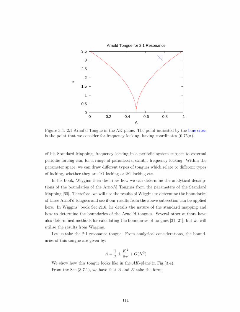
0
0.5
1
1.5
2
2.5
3
3.5
0 0.2 0.4 0.6 0.8 1
K
A
Arnold Tongue for 2:1 Resonance
Figure 3.4: 2:1 Arnol’d Tongue in the AK-plane. The point indicated by the blue crossis the point that we consider for frequency locking, having coordinates (0.75,π).
of his Standard Mapping, frequency locking in a periodic system subject to external
periodic forcing can, for a range of parameters, exhibit frequency locking. Within the
parameter space, we can draw different types of tongues which relate to different types
of locking, whether they are 1:1 locking or 2:1 locking etc.
In his book, Wiggins then describes how we can determine the analytical descrip-
tions of the boundaries of the Arnol’d Tongues from the parameters of the Standard
Mapping [60]. Therefore, we will use the results of Wiggins to determine the boundaries
of these Arnol’d tongues and see if our results from the above subsection can be applied
here. In Wiggins’ book Sec.21.6, he details the nature of the standard mapping and
how to determine the boundaries of the Arnol’d tongues. Several other authors have
also determined methods for calculating the boundaries of tongues [31, 21], but we will
utilise the results from Wiggins.
Let us take the 2:1 resonance tongue. From analytical considerations, the bound-
aries of this tongue are given by:
A =1
2± K2
8π+ O(K3)
We show how this tongue looks like in the AK-plane in Fig.(3.4).
From the Sec.(3.7.1), we have that A and K take the form:
111
A =Ω− ν
ν(3.116)
K =2ǫα∗πΩ
√
Ω2 cos2(φc) + ν2 sin2(φc)
Ω2 − ν2sin
(
πΩ
ν
)
(3.117)
Therefore, Eqn.(3.116) implies that:
Ω = (A + 1)ν (3.118)
Hence we can obtain an expression for ǫα∗ using Eqns.(3.117) and (3.118) to give:
ǫα∗ =K((A + 1)2 − 1)
2π(A + 1) sin(π(A + 1))√
(A + 1)2 cos2(φc) + sin2(φc)
Let us consider a non-trivial point within the tongue, and by non-trivial we mean
that A 6= 12 . We choose the point (A,K) = (0.75, π) as indicated in Fig.(3.4). This
implies that, from Eqn.(3.118) we have:
Ω =7
4ν
Also, if we take that φc = π, then Eqn.(3.7.2) gives us:
ǫα∗ =K((A + 1)2 − 1)
2π(A + 1)2 sin(π(A + 1))
⇒ ǫα∗ =33
49√
2⇒ ǫα∗ ≈ −0.476215
So, if our singular perturbation is indeed correct, we should find that the Poincare
mapping of equation governing the evolution of the correction to the time variable gives
us one point. This equation is:
dθ
dτ= ǫα0 cos(Ωt + φr) + O(ǫ2)
⇒ dθ
dt= ǫα∗ cos(ν(t + θ(t)) + φc) cos(Ωt + φr) + O(ǫ2) (3.119)
Numerically, Eqn.(3.119) is solved using:
θn+1 = θn + ∆tǫα∗ cos(ν(t + θn) + φc) cos(Ωt + φr) (3.120)
where ∆t is the timestep.
We show in Fig.(3.5), the Poincare mapping for this iterative scheme with the
parameters as detailed. We can clearly see that we do not get a frequency locked
solution. We must therefore conclude that we can not detect frequency locking using
the order of accuracy implemented into the above scheme.
112
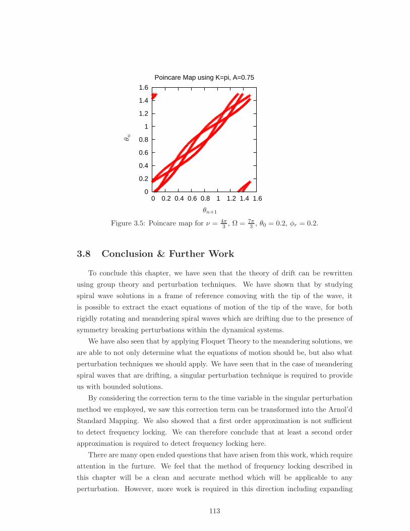
0
0.2
0.4
0.6
0.8
1
1.2
1.4
1.6
0 0.2 0.4 0.6 0.8 1 1.2 1.4 1.6
Poincare Map using K=pi, A=0.75
θn+1
θ n
Figure 3.5: Poincare map for ν = 4π3 , Ω = 7π
3 , θ0 = 0.2, φr = 0.2.
3.8 Conclusion & Further Work
To conclude this chapter, we have seen that the theory of drift can be rewritten
using group theory and perturbation techniques. We have shown that by studying
spiral wave solutions in a frame of reference comoving with the tip of the wave, it
is possible to extract the exact equations of motion of the tip of the wave, for both
rigidly rotating and meandering spiral waves which are drifting due to the presence of
symmetry breaking perturbations within the dynamical systems.
We have also seen that by applying Floquet Theory to the meandering solutions, we
are able to not only determine what the equations of motion should be, but also what
perturbation techniques we should apply. We have seen that in the case of meandering
spiral waves that are drifting, a singular perturbation technique is required to provide
us with bounded solutions.
By considering the correction term to the time variable in the singular perturbation
method we employed, we saw this correction term can be transformed into the Arnol’d
Standard Mapping. We also showed that a first order approximation is not sufficient
to detect frequency locking. We can therefore conclude that at least a second order
approximation is required to detect frequency locking here.
There are many open ended questions that have arisen from this work, which require
attention in the furture. We feel that the method of frequency locking described in
this chapter will be a clean and accurate method which will be applicable to any
perturbation. However, more work is required in this direction including expanding
113
the system to include second order terms.
114
Chapter 4
Initial Numerical Analysis
4.1 Introduction
In this chapter, we shall discuss the initial numerical analysis of the drift and me-
ander of spiral waves. The role of the analysis is to motivate subsequent chapters.
This chapter is concerned mainly with the drift of spiral waves. We shall split it
into two main parts: Inhomogeneity Induced Drift; and Electrophoresis Induced Drift.
We also note that we will use only Barkley’s model in this analysis.
For Inhomogeneity induced drift, we shall test the analytical theory that the velocity
of the drift of a rigidly rotating spiral wave should be linearly proportional to the drift
parameter [14]. We will also investigate whether the generic forms of the equations
of motion can be determined numerically for both rigidly rotating spiral waves and
meandering spiral waves, and touch on whether we can detect frequency locking.
For Electrophoresis induced drift, we shall conduct some analysis into frequency
locking within Barkley’s model.
All simulations were conducted using EZ-Spiral, amended accordingly for the pur-
poses of the study.
4.2 Inhomogeneity Induced Drift of Spiral Wave
When a wave drifts due to Inhomogeneities the model parameter(s) is(are) depen-
dent on the spatial coordinates. Its point of rotation is no longer stationary but drifts
along a straight line [14]. Therefore, as an example, we have that a = a(x) in Barkley’s
model. In our analysis, we took a to be linearly dependent on x to get:
a = a0 + a1x (4.1)
where a1 is known as the gradient of the drift. A formal analysis of this is done in
115
Chap.(3).
We will be using Barkley’s model throughout the simulations:
∂u
∂t= ∇2u +
1
εu(1− u)
[
u− v + b
a0 + a1x
]
(4.2)
∂v
∂t= u− v (4.3)
We will use EZ-Spiral throughout this analysis [6] and will firstly look at rigidly
rotating spiral waves.
4.2.1 Initial Analysis
We decided choose the following values of model parameters:
a0 = 0.7
a1 = 0
b = 0.15
ε = 0.01
noting that we initially do not have any drift. Other numerical and physical parameters
were chosen as follows:
Nx = 181
Lx = 60
Steps per plot = 16
ts = 0.8
where Nx is the number of grid points used for the numerical grid, L−x is the length of
the numerical box used, and ts is timestep as a fraction of the diffusion stability limit.
These are all specified in the task.dat file used with EZ-Spiral. This means that our
space step and time step were hx = 13 and ht = 1
30 respectively. These steps were kept
constant throughout our analysis. We also decided to use the Nine Point Laplacian
formula for solving the diffusion terms.
First of all we need to show that our amended EZ-Spiral ran correctly, having im-
plemented the changes for Inhomogeneity induced drift. We therefore ran the program
116
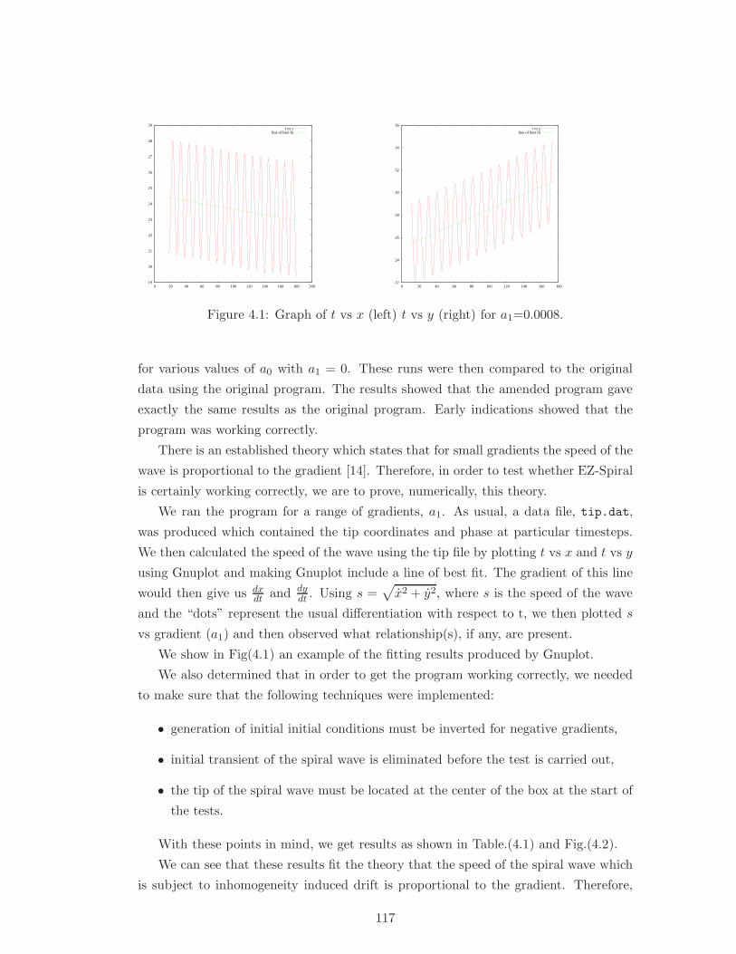
19
20
21
22
23
24
25
26
27
28
29
0 20 40 60 80 100 120 140 160 180 200
t vs xline of best fit
22
24
26
28
30
32
34
36
0 20 40 60 80 100 120 140 160 180
t vs yline of best fit
Figure 4.1: Graph of t vs x (left) t vs y (right) for a1=0.0008.
for various values of a0 with a1 = 0. These runs were then compared to the original
data using the original program. The results showed that the amended program gave
exactly the same results as the original program. Early indications showed that the
program was working correctly.
There is an established theory which states that for small gradients the speed of the
wave is proportional to the gradient [14]. Therefore, in order to test whether EZ-Spiral
is certainly working correctly, we are to prove, numerically, this theory.
We ran the program for a range of gradients, a1. As usual, a data file, tip.dat,
was produced which contained the tip coordinates and phase at particular timesteps.
We then calculated the speed of the wave using the tip file by plotting t vs x and t vs y
using Gnuplot and making Gnuplot include a line of best fit. The gradient of this line
would then give us dxdt
and dydt
. Using s =√
x2 + y2, where s is the speed of the wave
and the “dots” represent the usual differentiation with respect to t, we then plotted s
vs gradient (a1) and then observed what relationship(s), if any, are present.
We show in Fig(4.1) an example of the fitting results produced by Gnuplot.
We also determined that in order to get the program working correctly, we needed
to make sure that the following techniques were implemented:
• generation of initial initial conditions must be inverted for negative gradients,
• initial transient of the spiral wave is eliminated before the test is carried out,
• the tip of the spiral wave must be located at the center of the box at the start of
the tests.
With these points in mind, we get results as shown in Table.(4.1) and Fig.(4.2).
We can see that these results fit the theory that the speed of the spiral wave which
is subject to inhomogeneity induced drift is proportional to the gradient. Therefore,
117
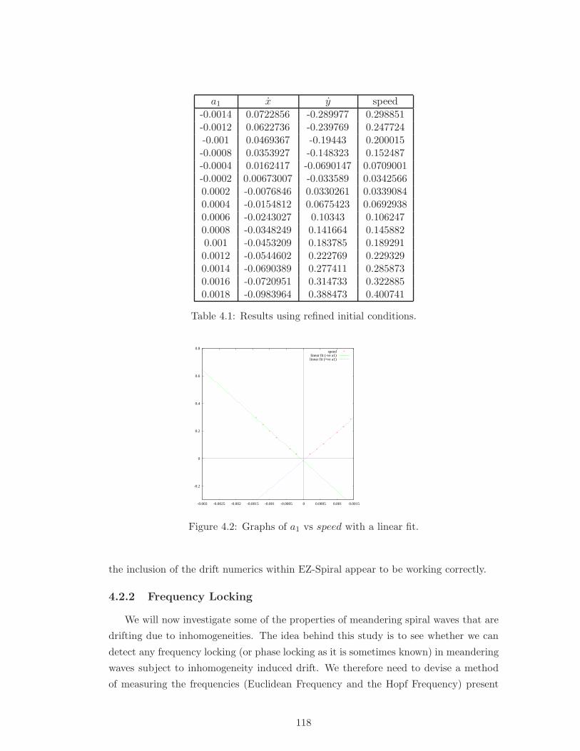
a1 x y speed
-0.0014 0.0722856 -0.289977 0.298851-0.0012 0.0622736 -0.239769 0.247724-0.001 0.0469367 -0.19443 0.200015-0.0008 0.0353927 -0.148323 0.152487-0.0004 0.0162417 -0.0690147 0.0709001-0.0002 0.00673007 -0.033589 0.03425660.0002 -0.0076846 0.0330261 0.03390840.0004 -0.0154812 0.0675423 0.06929380.0006 -0.0243027 0.10343 0.1062470.0008 -0.0348249 0.141664 0.1458820.001 -0.0453209 0.183785 0.1892910.0012 -0.0544602 0.222769 0.2293290.0014 -0.0690389 0.277411 0.2858730.0016 -0.0720951 0.314733 0.3228850.0018 -0.0983964 0.388473 0.400741
Table 4.1: Results using refined initial conditions.
-0.2
0
0.2
0.4
0.6
0.8
-0.003 -0.0025 -0.002 -0.0015 -0.001 -0.0005 0 0.0005 0.001 0.0015
speedlinear fit (-ve a1)linear fit (+ve a1)
Figure 4.2: Graphs of a1 vs speed with a linear fit.
the inclusion of the drift numerics within EZ-Spiral appear to be working correctly.
4.2.2 Frequency Locking
We will now investigate some of the properties of meandering spiral waves that are
drifting due to inhomogeneities. The idea behind this study is to see whether we can
detect any frequency locking (or phase locking as it is sometimes known) in meandering
waves subject to inhomogeneity induced drift. We therefore need to devise a method
of measuring the frequencies (Euclidean Frequency and the Hopf Frequency) present
118
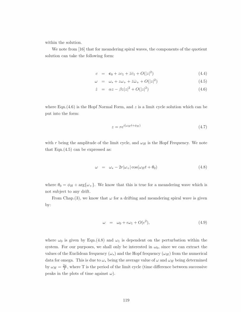
within the solution.
We note from [16] that for meandering spiral waves, the components of the quotient
solution can take the following form:
c = c0 + zc1 + zc1 + O(|z|2) (4.4)
ω = ω∗ + zω+ + zω+ + O(|z|2) (4.5)
z = αz − βz|z|2 + O(|z|2) (4.6)
where Eqn.(4.6) is the Hopf Normal Form, and z is a limit cycle solution which can be
put into the form:
z = rei(ωH t+φH) (4.7)
with r being the amplitude of the limit cycle, and ωH is the Hopf Frequency. We note
that Eqn.(4.5) can be expressed as:
ω = ω∗ − 2r|ω+| cos(ωHt + θ0) (4.8)
where θ0 = φH + argω+. We know that this is true for a meandering wave which is
not subject to any drift.
From Chap.(3), we know that ω for a drifting and meandering spiral wave is given
by:
ω = ω0 + ǫω1 + O(ǫ2), (4.9)
where ω0 is given by Eqn.(4.8) and ω1 is dependent on the perturbation within the
system. For our purposes, we shall only be interested in ω0, since we can extract the
values of the Euclidean frequency (ω∗) and the Hopf frequency (ωH) from the numerical
data for omega. This is due to ω∗ being the average value of ω and ωH being determined
by ωH = 2πT
, where T is the period of the limit cycle (time difference between successive
peaks in the plots of time against ω).
119
We calculate the quotient system by considering the equations of motion for the tip
of a spiral wave:
dR
dt= ceiΘ (4.10)
dΘ
dt= ω (4.11)
where, R = X + iY , and c = cx + icy . Rearranging, we get that:
cx(t) =dX
dtcos(Θ) +
dY
dtsin(Θ) (4.12)
cy(t) = −dX
dtsin(Θ) +
dY
dtcos(Θ) (4.13)
ω(t) =dΘ
dt(4.14)
So, after a simulation, we are given the tip coordinates, (X,Y ), and the phase of
the tip, Θ, for a range of times. We can therefore, numerically differentiate the given
tip data to find dXdt
, dYdt
, and dΘdt
, and hence find the corresponding values of cx, cy and
ω.
However, we note that we have used a numerical scheme to generate this data, and
with numerical schemes comes numerical errors (noise). Upon differentiating this data,
which contains the numerical noise, we are effectively amplifying the noise.
We bypass this hurdle by using a Tikhonov Regularisation method to “smoothen
out” the numerical data, before differentiating it. The type of regularisation method
we use is The Double Sweep Method (or Progonka in Russian) [27] to solve a finite
differences boundary value problem. This is a very easy and fast method to implement
into a C code.
Also, as with any regularisation method, there is a regularisation parameter. We
fixed this parameter at λreg = 1.0 throughout these calculations. This value gave us
the desired results for ω. One of the side affects of using a regularisation method, is
the suppressing of the amplitude of the limit cycle. However, we are not, for this study,
interested in the amplitude of the limit cycles, but just the values of ω∗ and ωH , which
are not affected by the regularisation technique.
So having regularised the data, we are able to differentiate it and use the results to
calculate the quotient solution.
We decided to investigate whether there is any frequency locking around a 4:3
resonance point. This is where the Hopf Frequency is four thirds larger than the
Euclidean frequency. A typical trajectory around this point is shown in Fig.(4.3).
120
1
2
3
4
5
6
7
8
9
10
11
2 3 4 5 6 7 8 9 10 11
Trajectory
Figure 4.3: Meandering Spiral Wave drifting due to inhomogeneities, passing througha point of resonance.
What is interesting about this is the apparent sudden change of direction around
the area of the point (4, 5). We are unable to provide a concrete answer to this problem,
but we suggest that this could be connected to the boundary conditions. If this is the
case, then we provide a solution to this in Chap.(5) where we solve the system in a
frame of reference which is comoving with the tip of the spiral wave. The methods
described in that chapter enable us to study the spiral wave solution in the knowledge
that the boundaries do not affect the dynamics of the spiral wave. Also, it provides
us with a tool which we can let run for as long as we desire (given computer hardware
constraints), since the tip of the spiral wave does not actually ever reach the boundary
of the box.
Regularising this data, we find that the quotient solution is shown in Fig.(4.4). One
of the points to note here is the presence of the strange deviation from the main limit
cycle. What we can rule out is that it is not associated with the initial transient of the
spiral wave, but provides an interesting phenominem for further study.
It is not very obvious whether there is any frequency locking present here. Therefore,
we shall look at the direction of the translational velocities in the laboratory frame of
reference (i.e. dXdt
and dYdt
). The idea behind this is that if there was any locking at all,
then we would observe that the translational acceleration would be zero for a particular
length of time.
We show the velocities in Fig.(4.5).
In Fig.(4.6), we show a cross section of the plot of dxdt
against dydt
using dxdt
= −0.3.
The figure clearly shows how the values of dydt
change with time as the trajectory crosses
121
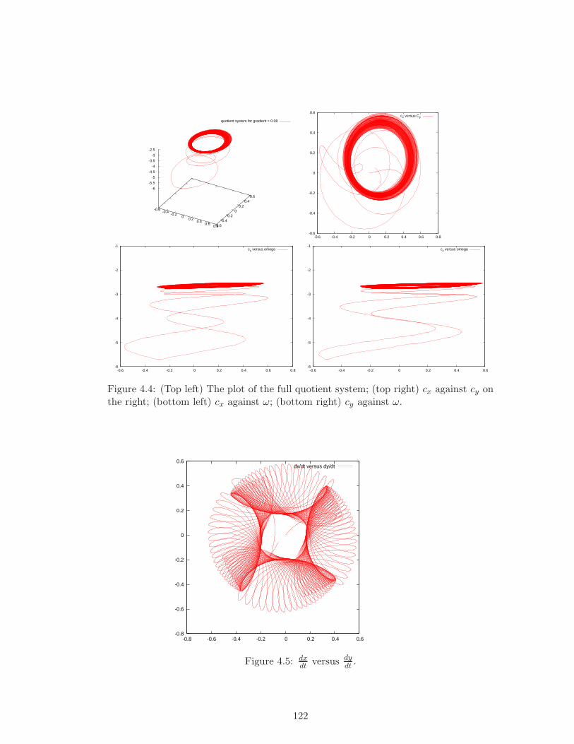
-0.6-0.4
-0.2 0
0.2 0.4
0.6 0.8-0.6
-0.4-0.2
0 0.2
0.4 0.6
-6
-5.5
-5
-4.5
-4
-3.5
-3
-2.5
quotient system for gradient = 0.08
-0.6
-0.4
-0.2
0
0.2
0.4
0.6
-0.6 -0.4 -0.2 0 0.2 0.4 0.6 0.8
cx versus Cy
-6
-5
-4
-3
-2
-1
-0.6 -0.4 -0.2 0 0.2 0.4 0.6 0.8
cx versus omega
-6
-5
-4
-3
-2
-1
-0.6 -0.4 -0.2 0 0.2 0.4 0.6
cx versus omega
Figure 4.4: (Top left) The plot of the full quotient system; (top right) cx against cy onthe right; (bottom left) cx against ω; (bottom right) cy against ω.
-0.8
-0.6
-0.4
-0.2
0
0.2
0.4
0.6
-0.8 -0.6 -0.4 -0.2 0 0.2 0.4 0.6
dx/dt versus dy/dt
Figure 4.5: dxdt
versus dydt
.
122
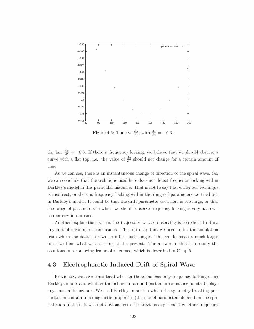
-0.415
-0.41
-0.405
-0.4
-0.395
-0.39
-0.385
-0.38
-0.375
-0.37
-0.365
-0.36
80 90 100 110 120 130 140 150 160
gradient = 0.008
Figure 4.6: Time vs dydt
, with dxdt
= −0.3.
the line dxdt
= −0.3. If there is frequency locking, we believe that we should observe a
curve with a flat top, i.e. the value of dydt
should not change for a certain amount of
time.
As we can see, there is an instantaneous change of direction of the spiral wave. So,
we can conclude that the technique used here does not detect frequency locking within
Barkley’s model in this particular instance. That is not to say that either our technique
is incorrect, or there is frequency locking within the range of parameters we tried out
in Barkley’s model. It could be that the drift parameter used here is too large, or that
the range of parameters in which we should observe frequency locking is very narrow -
too narrow in our case.
Another explanation is that the trajectory we are observing is too short to draw
any sort of meaningful conclusions. This is to say that we need to let the simulation
from which the data is drawn, run for much longer. This would mean a much larger
box size than what we are using at the present. The answer to this is to study the
solutions in a comoving frame of reference, which is described in Chap.5.
4.3 Electrophoretic Induced Drift of Spiral Wave
Previously, we have considered whether there has been any frequency locking using
Barkleys model and whether the behaviour around particular resonance points displays
any unusual behaviour. We used Barkleys model in which the symmetry breaking per-
turbation contain inhomogenetic properties (the model parameters depend on the spa-
tial coordinates). It was not obvious from the previous experiment whether frequency
123
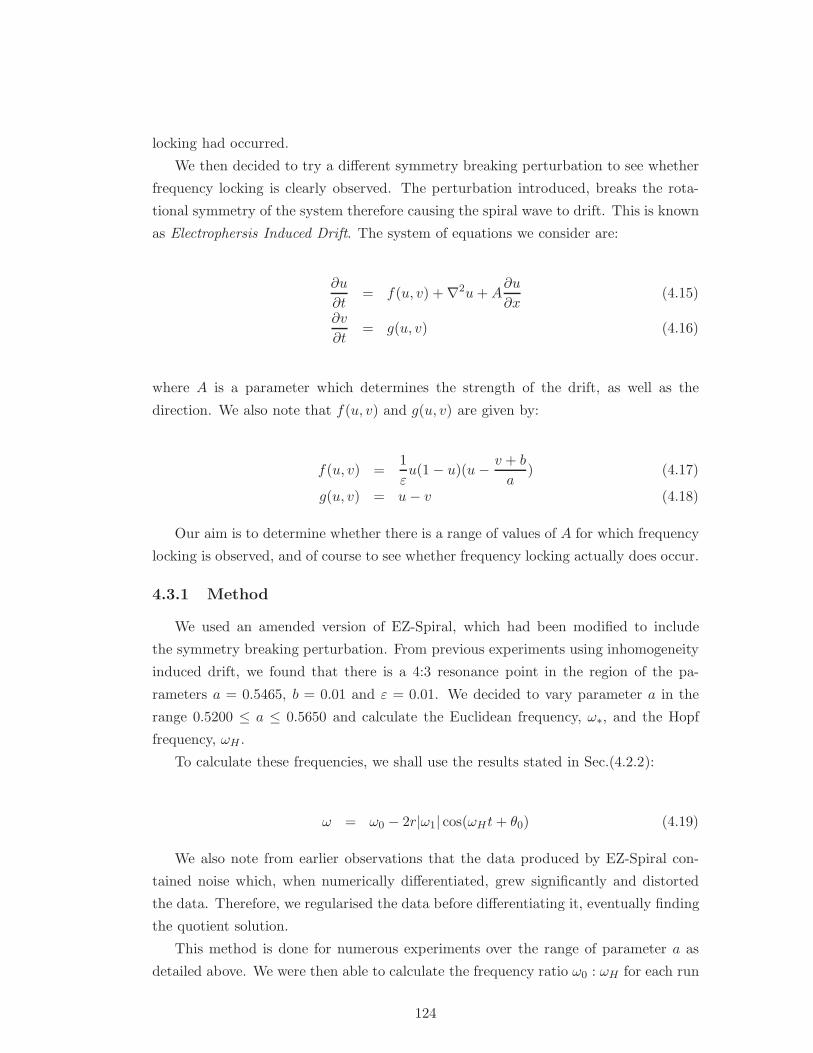
locking had occurred.
We then decided to try a different symmetry breaking perturbation to see whether
frequency locking is clearly observed. The perturbation introduced, breaks the rota-
tional symmetry of the system therefore causing the spiral wave to drift. This is known
as Electrophersis Induced Drift. The system of equations we consider are:
∂u
∂t= f(u, v) +∇2u + A
∂u
∂x(4.15)
∂v
∂t= g(u, v) (4.16)
where A is a parameter which determines the strength of the drift, as well as the
direction. We also note that f(u, v) and g(u, v) are given by:
f(u, v) =1
εu(1− u)(u− v + b
a) (4.17)
g(u, v) = u− v (4.18)
Our aim is to determine whether there is a range of values of A for which frequency
locking is observed, and of course to see whether frequency locking actually does occur.
4.3.1 Method
We used an amended version of EZ-Spiral, which had been modified to include
the symmetry breaking perturbation. From previous experiments using inhomogeneity
induced drift, we found that there is a 4:3 resonance point in the region of the pa-
rameters a = 0.5465, b = 0.01 and ε = 0.01. We decided to vary parameter a in the
range 0.5200 ≤ a ≤ 0.5650 and calculate the Euclidean frequency, ω∗, and the Hopf
frequency, ωH .
To calculate these frequencies, we shall use the results stated in Sec.(4.2.2):
ω = ω0 − 2r|ω1| cos(ωHt + θ0) (4.19)
We also note from earlier observations that the data produced by EZ-Spiral con-
tained noise which, when numerically differentiated, grew significantly and distorted
the data. Therefore, we regularised the data before differentiating it, eventually finding
the quotient solution.
This method is done for numerous experiments over the range of parameter a as
detailed above. We were then able to calculate the frequency ratio ω0 : ωH for each run
124
-2.76
-2.74
-2.72
-2.7
-2.68
-2.66
-2.64
-2.62
-2.6
-2.58
-2.56
96 98 100 102 104 106 108 110 112 114 116
t vs omline of best fit
-2.78
-2.76
-2.74
-2.72
-2.7
-2.68
-2.66
-2.64
-2.62
-2.6
-2.58
96 98 100 102 104 106 108 110 112 114 116
t vs omline of best fit
Figure 4.7: Plots of time vs. ω, with a0 = 0.5400, ω0 = -2.64982, ωH = 3.52981 (left),and a0 = 0.5530, ω0 = -2.67089, ωH = 3.55742 (right).
and plot the graph of a vs. ω0 : ωH . If frequency locking is present, then we should
observe that for a particular range of values of a, each a should have the same frequency
ratio.
4.3.2 Observations
We show below the results of the curve fitting exercise to show that the curve does
fit for the values that we require. As we noted, we need the value of ω0, which is the
average value of the graph, and ωH which is calculated as:
ωH =2π
T(4.20)
where T is the time between consecutive“peaks” on the graph.
We show in table (4.2) the values of the frequencies calculated and also their ratios
for A = 0.05
We show in Fig.(4.8) the plot of a against the frequency ratio.
Furthermore, we can see in Fig(4.9) that for a = 0.5530 it looks as though we have
locking. In fact Fig.(4.9) shows that the wave is still slightly rotating.
To finish off this part of our work, we show in Fig.(4.11) the results from a range
of values for A.
It is clear that for all these parameter values, we do not get frequency locking in our
simulations. As with inhomogeneity induced drift, perhaps evidence of locking could be
observed for longer trajectories but that would mean an increase in box size and related
increase in computational resources. Hence, a way around this would be to study the
solutions in a frame of reference comoving with the tip of the spiral wave (Chap.(5)).
125
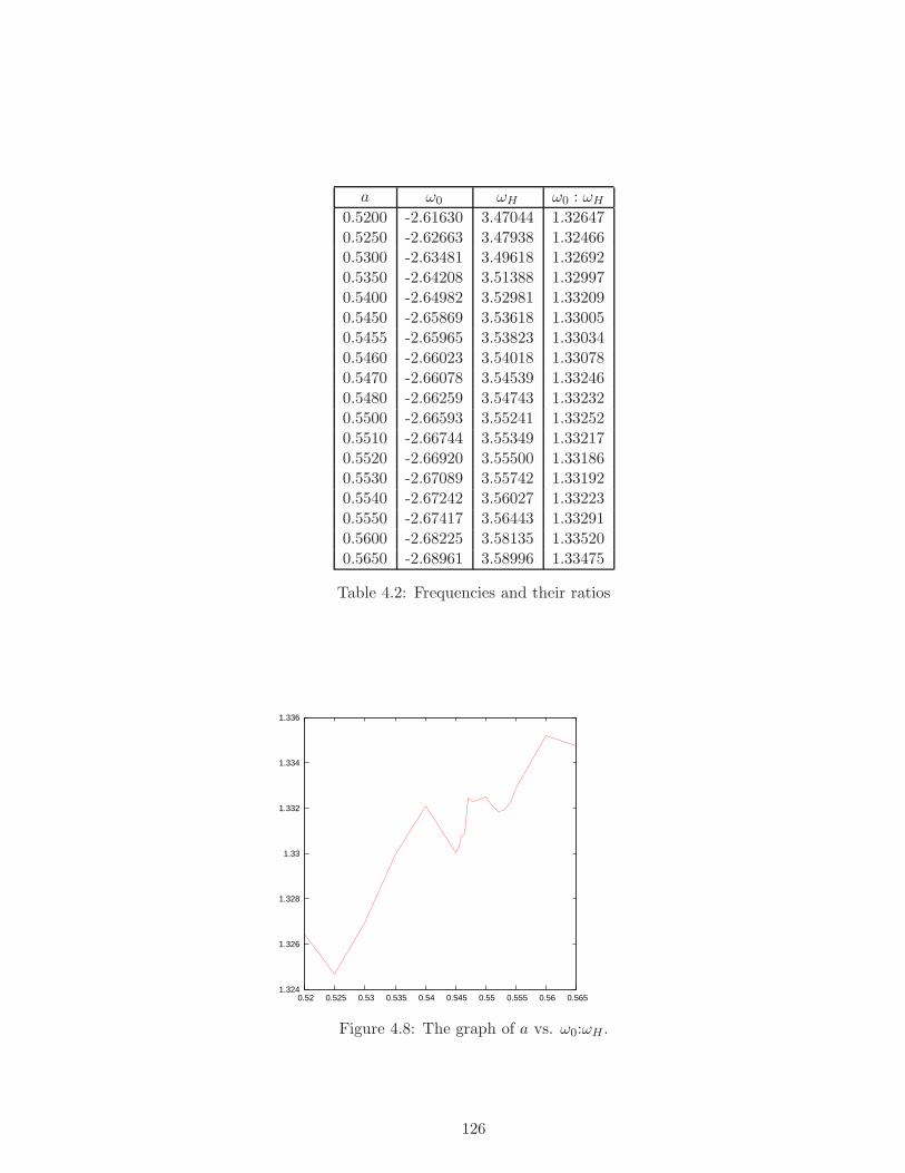
a ω0 ωH ω0 : ωH
0.5200 -2.61630 3.47044 1.326470.5250 -2.62663 3.47938 1.324660.5300 -2.63481 3.49618 1.326920.5350 -2.64208 3.51388 1.329970.5400 -2.64982 3.52981 1.332090.5450 -2.65869 3.53618 1.330050.5455 -2.65965 3.53823 1.330340.5460 -2.66023 3.54018 1.330780.5470 -2.66078 3.54539 1.332460.5480 -2.66259 3.54743 1.332320.5500 -2.66593 3.55241 1.332520.5510 -2.66744 3.55349 1.332170.5520 -2.66920 3.55500 1.331860.5530 -2.67089 3.55742 1.331920.5540 -2.67242 3.56027 1.332230.5550 -2.67417 3.56443 1.332910.5600 -2.68225 3.58135 1.335200.5650 -2.68961 3.58996 1.33475
Table 4.2: Frequencies and their ratios
1.324
1.326
1.328
1.33
1.332
1.334
1.336
0.52 0.525 0.53 0.535 0.54 0.545 0.55 0.555 0.56 0.565
Figure 4.8: The graph of a vs. ω0:ωH .
126
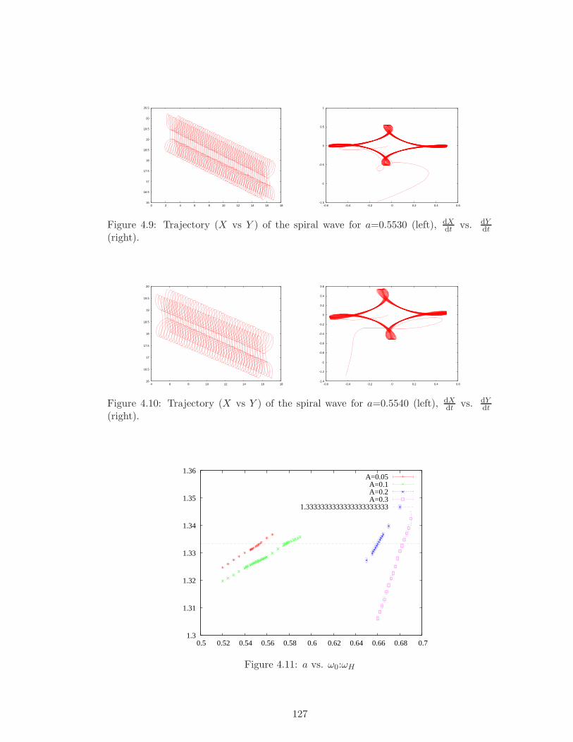
16
16.5
17
17.5
18
18.5
19
19.5
20
20.5
0 2 4 6 8 10 12 14 16 18-1.5
-1
-0.5
0
0.5
1
-0.6 -0.4 -0.2 0 0.2 0.4 0.6
Figure 4.9: Trajectory (X vs Y ) of the spiral wave for a=0.5530 (left), dXdt
vs. dYdt
(right).
16
16.5
17
17.5
18
18.5
19
19.5
20
4 6 8 10 12 14 16 18-1.4
-1.2
-1
-0.8
-0.6
-0.4
-0.2
0
0.2
0.4
0.6
-0.6 -0.4 -0.2 0 0.2 0.4 0.6
Figure 4.10: Trajectory (X vs Y ) of the spiral wave for a=0.5540 (left), dXdt
vs. dYdt
(right).
1.3
1.31
1.32
1.33
1.34
1.35
1.36
0.5 0.52 0.54 0.56 0.58 0.6 0.62 0.64 0.66 0.68 0.7
A=0.05A=0.1A=0.2A=0.3
1.3333333333333333333333
Figure 4.11: a vs. ω0:ωH
127
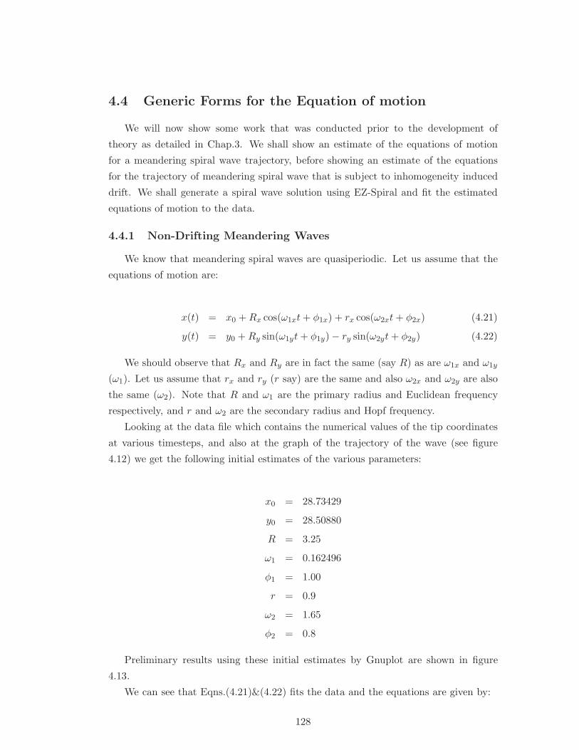
4.4 Generic Forms for the Equation of motion
We will now show some work that was conducted prior to the development of
theory as detailed in Chap.3. We shall show an estimate of the equations of motion
for a meandering spiral wave trajectory, before showing an estimate of the equations
for the trajectory of meandering spiral wave that is subject to inhomogeneity induced
drift. We shall generate a spiral wave solution using EZ-Spiral and fit the estimated
equations of motion to the data.
4.4.1 Non-Drifting Meandering Waves
We know that meandering spiral waves are quasiperiodic. Let us assume that the
equations of motion are:
x(t) = x0 + Rx cos(ω1xt + φ1x) + rx cos(ω2xt + φ2x) (4.21)
y(t) = y0 + Ry sin(ω1yt + φ1y)− ry sin(ω2yt + φ2y) (4.22)
We should observe that Rx and Ry are in fact the same (say R) as are ω1x and ω1y
(ω1). Let us assume that rx and ry (r say) are the same and also ω2x and ω2y are also
the same (ω2). Note that R and ω1 are the primary radius and Euclidean frequency
respectively, and r and ω2 are the secondary radius and Hopf frequency.
Looking at the data file which contains the numerical values of the tip coordinates
at various timesteps, and also at the graph of the trajectory of the wave (see figure
4.12) we get the following initial estimates of the various parameters:
x0 = 28.73429
y0 = 28.50880
R = 3.25
ω1 = 0.162496
φ1 = 1.00
r = 0.9
ω2 = 1.65
φ2 = 0.8
Preliminary results using these initial estimates by Gnuplot are shown in figure
4.13.
We can see that Eqns.(4.21)&(4.22) fits the data and the equations are given by:
128
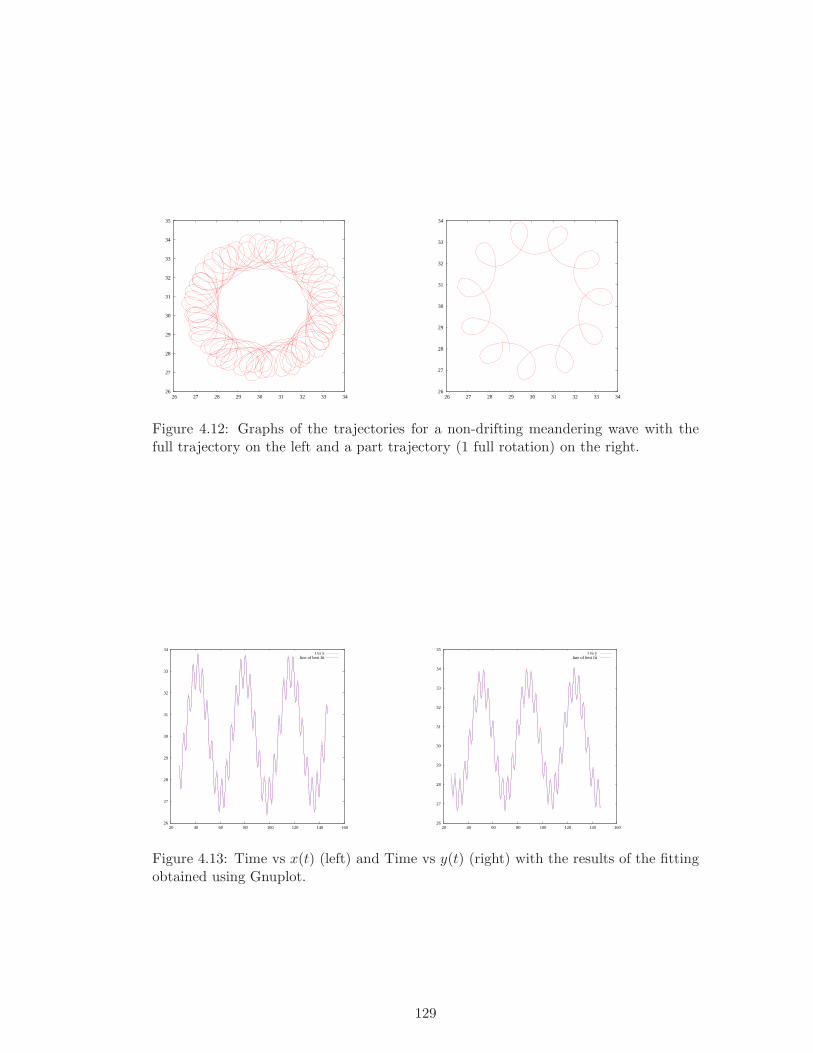
26
27
28
29
30
31
32
33
34
35
26 27 28 29 30 31 32 33 34 26
27
28
29
30
31
32
33
34
26 27 28 29 30 31 32 33 34
Figure 4.12: Graphs of the trajectories for a non-drifting meandering wave with thefull trajectory on the left and a part trajectory (1 full rotation) on the right.
26
27
28
29
30
31
32
33
34
20 40 60 80 100 120 140 160
t vs xline of best fit
26
27
28
29
30
31
32
33
34
35
20 40 60 80 100 120 140 160
t vs yline of best fit
Figure 4.13: Time vs x(t) (left) and Time vs y(t) (right) with the results of the fittingobtained using Gnuplot.
129
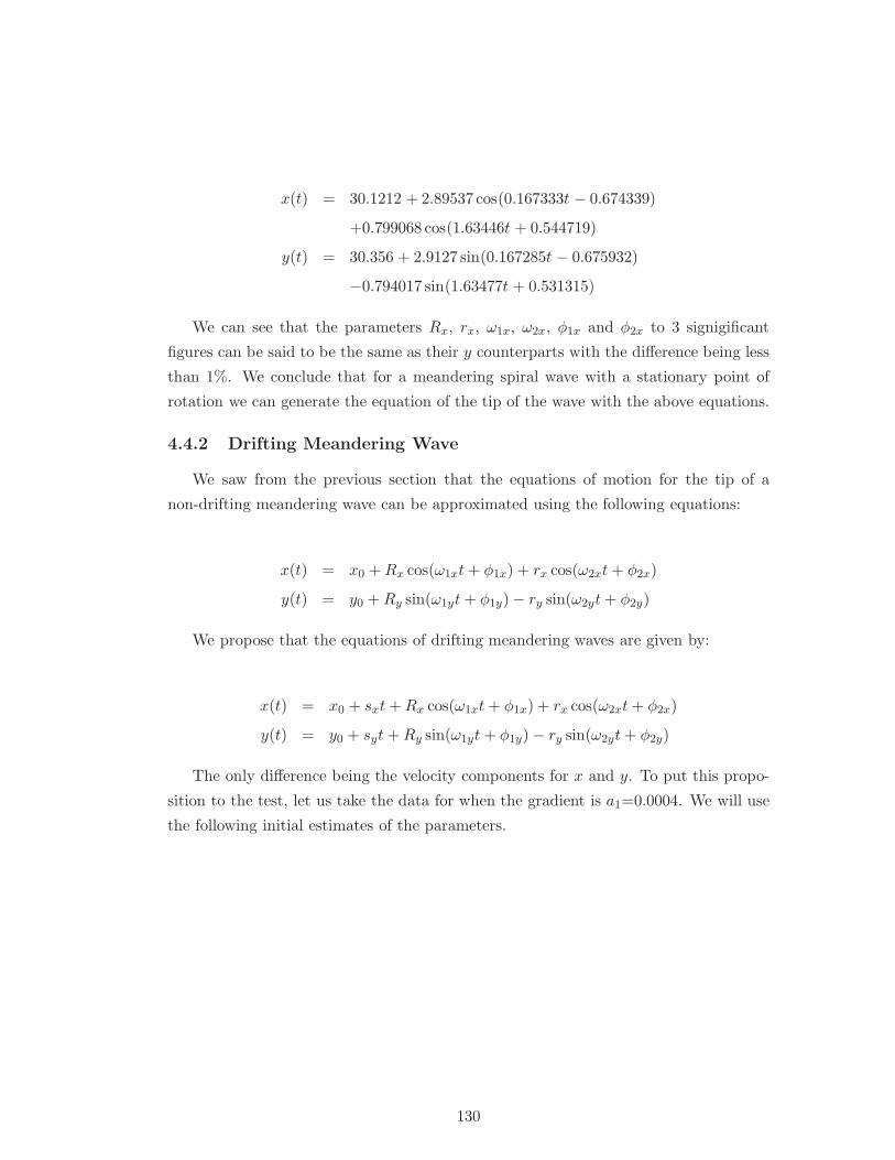
x(t) = 30.1212 + 2.89537 cos(0.167333t − 0.674339)
+0.799068 cos(1.63446t + 0.544719)
y(t) = 30.356 + 2.9127 sin(0.167285t − 0.675932)
−0.794017 sin(1.63477t + 0.531315)
We can see that the parameters Rx, rx, ω1x, ω2x, φ1x and φ2x to 3 signigificant
figures can be said to be the same as their y counterparts with the difference being less
than 1%. We conclude that for a meandering spiral wave with a stationary point of
rotation we can generate the equation of the tip of the wave with the above equations.
4.4.2 Drifting Meandering Wave
We saw from the previous section that the equations of motion for the tip of a
non-drifting meandering wave can be approximated using the following equations:
x(t) = x0 + Rx cos(ω1xt + φ1x) + rx cos(ω2xt + φ2x)
y(t) = y0 + Ry sin(ω1yt + φ1y)− ry sin(ω2yt + φ2y)
We propose that the equations of drifting meandering waves are given by:
x(t) = x0 + sxt + Rx cos(ω1xt + φ1x) + rx cos(ω2xt + φ2x)
y(t) = y0 + syt + Ry sin(ω1yt + φ1y)− ry sin(ω2yt + φ2y)
The only difference being the velocity components for x and y. To put this propo-
sition to the test, let us take the data for when the gradient is a1=0.0004. We will use
the following initial estimates of the parameters.
130
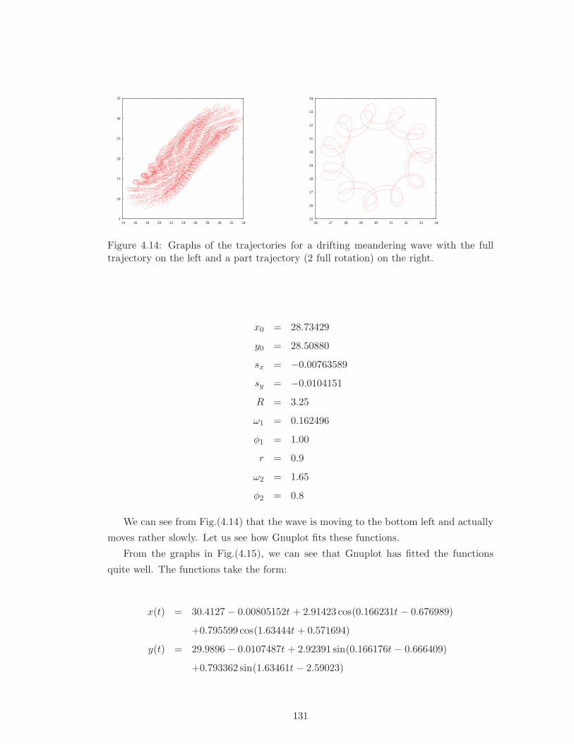
5
10
15
20
25
30
35
14 16 18 20 22 24 26 28 30 32 34 25
26
27
28
29
30
31
32
33
34
26 27 28 29 30 31 32 33 34
Figure 4.14: Graphs of the trajectories for a drifting meandering wave with the fulltrajectory on the left and a part trajectory (2 full rotation) on the right.
x0 = 28.73429
y0 = 28.50880
sx = −0.00763589
sy = −0.0104151
R = 3.25
ω1 = 0.162496
φ1 = 1.00
r = 0.9
ω2 = 1.65
φ2 = 0.8
We can see from Fig.(4.14) that the wave is moving to the bottom left and actually
moves rather slowly. Let us see how Gnuplot fits these functions.
From the graphs in Fig.(4.15), we can see that Gnuplot has fitted the functions
quite well. The functions take the form:
x(t) = 30.4127 − 0.00805152t + 2.91423 cos(0.166231t − 0.676989)
+0.795599 cos(1.63444t + 0.571694)
y(t) = 29.9896 − 0.0107487t + 2.92391 sin(0.166176t − 0.666409)
+0.793362 sin(1.63461t − 2.59023)
131
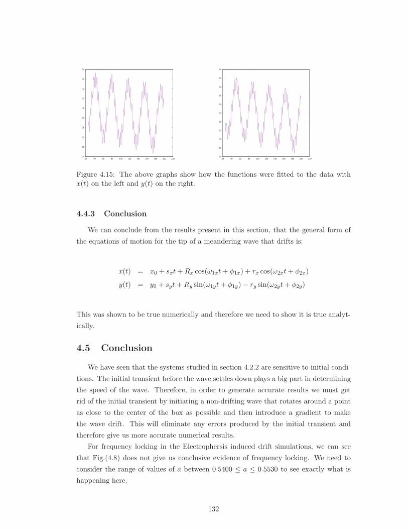
25
26
27
28
29
30
31
32
33
34
20 40 60 80 100 120 140 160 180 200 220 24
25
26
27
28
29
30
31
32
33
34
20 40 60 80 100 120 140 160 180 200 220
Figure 4.15: The above graphs show how the functions were fitted to the data withx(t) on the left and y(t) on the right.
4.4.3 Conclusion
We can conclude from the results present in this section, that the general form of
the equations of motion for the tip of a meandering wave that drifts is:
x(t) = x0 + sxt + Rx cos(ω1xt + φ1x) + rx cos(ω2xt + φ2x)
y(t) = y0 + syt + Ry sin(ω1yt + φ1y)− ry sin(ω2yt + φ2y)
This was shown to be true numerically and therefore we need to show it is true analyt-
ically.
4.5 Conclusion
We have seen that the systems studied in section 4.2.2 are sensitive to initial condi-
tions. The initial transient before the wave settles down plays a big part in determining
the speed of the wave. Therefore, in order to generate accurate results we must get
rid of the initial transient by initiating a non-drifting wave that rotates around a point
as close to the center of the box as possible and then introduce a gradient to make
the wave drift. This will eliminate any errors produced by the initial transient and
therefore give us more accurate numerical results.
For frequency locking in the Electrophersis induced drift simulations, we can see
that Fig.(4.8) does not give us conclusive evidence of frequency locking. We need to
consider the range of values of a between 0.5400 ≤ a ≤ 0.5530 to see exactly what is
happening here.
132
It would also be useful to see what the graph would look like for other values of A
and hopefully produce the “Arnold Tongue” for this resonance in Barkleys model, if it
exists.
133
Chapter 5
Numerical Solutions of SpiralWaves in a Moving Frame ofReference
5.1 Introduction
This chapter is concerned with the numerical solution to the Reaction-Diffusion-
Advection system of equations for spiral wave solutions. As mentioned previously, such
solutions are spiral wave solutions in a frame of reference that is comoving with the tip
of the wave.
The motivation behind this work stemmed from our initial analysis into the drift
of meandering spiral waves, subject to symmetry breaking perturbations. In our initial
analysis in the laboratory frame of reference, we noted that in certain instances when
the drift was “fast”, the spiral wave reached the boundary very quickly. So, a much
larger box size was needed in order to try to extract any meaningful results.
Therefore, our solution to this was to use a frame of reference that was comoving
with the tip of the wave (referred to for the rest of this chapter as the “comoving
frame”). This would mean that the tip of the wave would never reach the boundary
of the box and therefore we could run the program for as long as we wished, safe in
the knowledge that the wave would never reach the boundary. Also, we could afford a
smaller box size in order to gain faster numerical calculations, provided of course that
the box size is not too small such that the boundaries have an effect.
This area has been regarded previously by Beyn & Thummler, who used a Center
Bundle Reduction approach to generated the equations of motion of the top of the
spiral wave [13]. However, although they managed to pin a rigidly rotating spiral wave,
they found it very difficult to pin a periodic (meandering) solution. We will show that
it is possible to pin a meandering solution and show this in the examples section.
In the first section of this chapter, we will discuss the numerical implementation
134
of this problem, and discuss the hurdles we had to overcome and how we overcame
them. This implementation resulted in a new program called “EZ-Freeze”, which is an
amended version of “EZ-Spiral” [6]. We will then show two examples using EZ-Freeze;
one for a rigidly rotating spiral wave in Barkley’s model, and one for a meandering
spiral wave in FHN.
We then discuss the accuracy of EZ-Freeze by showing results from our convergence
analysis, before moving onto to two further applications of EZ-Freeze; viz. studies into
1:1 resonance for meandering spiral waves, and large core rigidly rotating spiral waves.
We conclude the chapter with a summary of the results, methods developed and
questions for the future.
This chapter is based on results which are currently in preparation to be published
[26].
5.2 Numerical Implementation
We will be looking at the numerical solution to the Reaction-Diffusion-Advection
system of equations as derived in Chap.3. The system of equations derived there
(Eqns.(3.22)-(3.22)) is reminded below:
∂v
∂t= D∇2v + f(v) + (c,∇)v + ω
∂v
∂θ+ ǫh(v, r, t) (5.1)
v1(R, t) = u∗ (5.2)
v2(R, t) = v∗ (5.3)
∂v1(R, t)
∂x= 0 (5.4)
with v,R, f, h ∈ R2, and f(v) are the local kinetics. We shall consider two models, the
FHN model [24, 49]:
∂u
∂t= ∇2u +
1
ε
(
u− u3
3− v
)
+ (c,∇)u + ω∂u
∂θ+ ǫhu(u, v, x, y, t)
∂v
∂t= Dv∇2v + ε(u + β − γv) + (c,∇)v + ω
∂v
∂θ+ ǫhv(u, v, x, y, t)
u(R, t) = u∗
v(R, t) = v∗∂u(R, t)
∂x= 0
and Barkley’s model [11]:
∂u
∂t= ∇2u +
1
εu(1− u)
[
u− v + b
a
]
+ (c,∇)u + ω∂u
∂θ+ ǫhu(u, v, x, y, t)
∂v
∂t= Dv∇2v + (u− v) + (c,∇)v + ω
∂v
∂θ+ ǫhv(u, v, x, y, t)
135
u(R, t) = u∗
v(R, t) = v∗∂u(R, t)
∂x= 0
where hu and hv are the u and v components of the perturbation h, i.e. h = (hu, hv),
and Dv is the ratio of diffusion coefficients, which in all our numerical simulations, is
taken to be Dv = 0.
This system was derived in Chap.(3) during our analytical work. In the first part
of our work we shall consider the case when ǫ = 0, but we will also consider ǫ 6= 0 later
on in this section.
We will call Eqns.(5.2)-(5.4) the tip pinning conditions, and it is these three con-
ditions which define the Representative Manifold that we introduced in Chap.3. The
system of Eqns.(5.1)-(5.4) will be called the Quotient System, with the phase space
M = v, c, ω. For brevity, we will call the c and ω components of the Quotient
System Solution, the Quotient Solution. If we had just Eqn.(5.1), then we would have
just 2 equations for 5 unknowns. Therefore, the tip pinning conditions, together with
Eqn.(5.1), give us a closed system of equations.
We shall see in Sec.(5.2.3) that the above tip pinning conditions do not give accu-
rate calculations of ω, and therefore we will be using refined conditions which will be
introduced and described in detail in that section.
Let us consider the physical interpretation of the advection terms. The reaction
and diffusion parts of the system, can give us a spiral wave solution (for particularly
chosen parameters and initial conditions), and in the absence of advection, the solution
will be in the laboratory frame of reference. The advection terms, for carefully chosen
advection coefficients (c, ω), actually move the frame of reference such that it is moving
with the tip of the spiral wave. So, the crucial point to note here is that the spiral wave
in the comoving frame is simply the spiral wave in the laboratory frame transformed so
that the tip is in a particular position and with a particular phase (these are discussed
below).
So, the idea we have in this part of our research, is to use operator splitting. We take
a spiral wave solution as generated using the numerical methods adopted by Dwight
Barkley in EZ-Spiral [8, 6], and then use the following methods detailed below to solve
the advection terms. Therefore, the numerical equations to solve are:
vn+ 1
2i,j = vn
i,j + ∆tR(vni,j) + O(∆2
t )
vn+1i,j = v
n+ 12
i,j + ∆tA(vn+ 1
2i,j ) + O(∆2
t )
136
where vni,j is v at the n-th time step and at the grid coordinate (i, j), and R and A are
the Reaction-Diffusion and Advection terms respectively, and ∆t is the time step. We
note here that we have used an explicit, forward Euler method to first order accuracy
to calculate the time derivatives.
Let us consider the numerical methods implemented in the Reaction-Diffusion part
of the system. We shall be using a first order accurate forward Euler method to calculate
the temporal derivatives, and the Five Point Laplacian method for the Laplacian. These
are all detailed extensively in [8].
Let R = (X,Y ) be the tip coordinates. Now, we choose c and ω such that the tip
of the wave remains in a fixed position and at a fixed orientation for all time. This
means that R is fixed and we are free to choose the fixed value of R as we feel fit. We
choose to fix R at the center of the box. This would mean that the tip is the maximum
possible distance away from any boundary. We also take the center of the box to be
the origin, and therefore we have that R = (0, 0).
So, how exactly do we numerically solve the second step (5.5) above? The differen-
tial equation is:
∂vn+1
∂t= cx
∂vn+ 12
∂x+ cy
∂vn+ 12
∂y+ ω
∂vn+ 12
∂θ(5.5)
There are two main calculations that we must do which are coupled. Firstly we
must calculate the advection coefficients, cx, cy, and ω. Secondly, we need to calculate
the spatial derivatives which appear in (5.5). Although the two are connected, we will
describe the methods to solve these separately.
5.2.1 Advection Coefficients: cx, cy, and ω
We devised two methods to calculate cx, cy and ω, which we will describe in detail
in the following pages. The first method (Method 1) involves measuring how far the
tip of the wave has traveled after the first half step and determining what cx, cy and ω
are needed in order to bring back the tip to the desired position. The second method
(Method 2) is a more concrete and accurate method which involves the solution to a
system of three linear equations 1.
Method 1: Shifts in the Euclidean Space.
Consider now the spiral wave solution in the first half step, and assume that the
solution, vn, i.e. the solution before the first half step is applied, had its tip at the
desired position (X,Y ), and with the desired orientation, Θ, Fig.(5.1).
1This method was suggested by Dr B. Vasiev, Mathematical Sciences, University of Liverpool
137
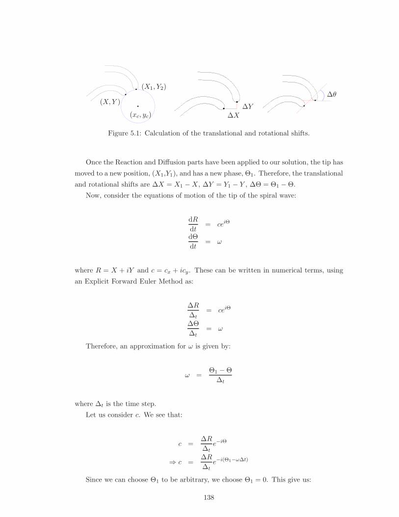
(X,Y )
(X1, Y2)
(xc, yc) ∆X∆Y
∆θ
Figure 5.1: Calculation of the translational and rotational shifts.
Once the Reaction and Diffusion parts have been applied to our solution, the tip has
moved to a new position, (X1,Y1), and has a new phase, Θ1. Therefore, the translational
and rotational shifts are ∆X = X1 −X, ∆Y = Y1 − Y , ∆Θ = Θ1 −Θ.
Now, consider the equations of motion of the tip of the spiral wave:
dR
dt= ceiΘ
dΘ
dt= ω
where R = X + iY and c = cx + icy. These can be written in numerical terms, using
an Explicit Forward Euler Method as:
∆R
∆t= ceiΘ
∆Θ
∆t= ω
Therefore, an approximation for ω is given by:
ω =Θ1 −Θ
∆t
where ∆t is the time step.
Let us consider c. We see that:
c =∆R
∆te−iΘ
⇒ c =∆R
∆te−i(Θ1−ω∆t)
Since we can choose Θ1 to be arbitrary, we choose Θ1 = 0. This give us:
138
∆R
∆t= ce−iω∆t
∆R
∆t= c(1 + O(∆t))
Hence we have:
c =R1 −R
∆t
Summarizing, we have:
ω =Θ1 −Θ
∆t
cx =X1 −X
∆t
cy =Y1 − Y
∆t
Hence, we have a first order accurate scheme to calculate the quotient system, which
is straight forward and quick. However, as we shall see in the examples following, it is
unstable.
Method 2: Solution to a System of Linear Equations in cx, cy and ω.
We now consider creating a system of linear equations which can be solved to give
us the quotient system. We have three unknowns; cx, cy and ω. Therefore, we require
three linear equations in cx, cy and ω. We derive these equations from Eqn.(5.5), and
also consider the tip pinning conditions (5.2)-(5.4). We note that in these tip pinning
conditions, we consider when the tip is at the origin, R = (0, 0).
Consider for a moment the tip pinning conditions:
v1(0, 0, t) = u∗
v2(0, 0, t) = v∗∂v1(0, 0, t)
∂x= 0
The first two are fairly straight forward to understand. They say that the values of
v1 and v2 at the desired position are fixed for all time. The third condition, says:
∂v1(0, 0, t)
∂x= 0
v1(∆x, 0, t) − v1(0, 0, t)
∆x= 0
⇒ v1(∆x, 0, t) = v1(0, 0, t)
139
Therefore, the third pinning condition interprets as the value of v1 at the grid point
in the x-direction next to the desired point is the same as that at the desired point.
So, our linear system of three equations considers the values of v1 at the desired point
and the point next to it, and also the value of v2 at the desired point, giving:
∂v1(0, 0, t)
∂t= cx
∂v1(0, 0, t)
∂x+ cy
∂v1(0, 0, t)
∂y+ ω
∂v1(0, 0, t)
∂θ
∂v2(0, 0, t)
∂t= cx
∂v2(0, 0, t)
∂x+ cy
∂v2(0, 0, t)
∂y+ ω
∂v2(0, 0, t)
∂θ
∂v1(∆x, 0, t)
∂t= cx
∂v1(∆x, 0, t)
∂x+ cy
∂v1(∆x, 0, t)
∂y
+ω∂v1(∆x, 0, t)
∂θ
We note that the derivatives with respect to θ can be rewritten as:
∂θ = x∂y − y∂x
and we also denote v1(∆x, 0, t) = v1(0, 0, t).
Next, we use the tip pinning conditions and find that the linear system now becomes:
∂v1(0, 0, t)
∂t= cx
∂v1(0, 0, t)
∂x+ cy
∂v1(0, 0, t)
∂y
∂v2(0, 0, t)
∂t= cx
∂v2(0, 0, t)
∂x+ cy
∂v2(0, 0, t)
∂y
∂v1(0, 0, t)
∂t= cx
∂v1(0, 0, t)
∂x+ cy
∂v1(0, 0, t)
∂y+ ω∆x
∂v1(0, 0, t)
∂y
These are then easily solved using linear algebra to give:
cx =∂xv1(0, 0, t)∂tv2(0, 0, t) − ∂xv2(0, 0, t)∂tv1(0, 0, t)
∂xv1(0, 0, t)∂yv2(0, 0, t) − ∂yv1(0, 0, t)∂xv2(0, 0, t)
cy =∂yv1(0, 0, t)∂tv2(0, 0, t) − ∂yv2(0, 0, t)∂tv1(0, 0, t)
∂xv1(0, 0, t)∂yv2(0, 0, t) − ∂yv1(0, 0, t)∂xv2(0, 0, t)
ω =∂tv1(0, 0, t) − cx∂xv1(0, 0, t) − cy∂yv1(0, 0, t)
∆x∂yv1(0, 0, t)
where ∂x represents partial differentiation with respect to x; similarly for y and t.
As we have already mentioned, it is possible to solve this system since we already
know the solution vn+ 12 .
In order to implement this system into our code, we must now discuss how we can
approximate the spatial derivatives.
140
5.2.2 Numerical Approximation of the Spatial Derivatives
First, we implemented an explicit, upwind Euler method:
α∂v(x, y, t)
∂x= α
v(x + ∆x, y, t)− v(x, y, t)
∆x+ O(∆2
x) if α > 0
α∂v(x, y, t)
∂x= α
v(x, y, t) − v(x−∆x, y, t)
∆x+ O(∆2
x) if α < 0
where ∆x is the shift in the x-direction. Note that we do not need to consider when
the advection coefficient is α = 0 in the above equations, since α = 0 means that the
particular advection will not be present!
As we will show in the next section section, this approximation is not accurate
enough and therefore we need a second order scheme. We therefore implement a second
order accurate, explicit upwind scheme which is given below [17]:
α∂u
∂x
∣
∣
∣
∣
(x,y)
≈ α
2∆x
(−3u(x, y) + 4u(x + ∆x, y)− u(x + 2∆x, y)) α > 0
or α∂u
∂x
∣
∣
∣
∣
(x,y)
≈ α
2∆x(3u(x, y)− 4u(x + ∆x, y) + u(x− 2∆x, y)) α < 0
5.2.3 Tip Pinning Conditions
As mentioned earlier, we found that the calculation of the quotient system using
the tip pinning conditions (5.2)-(5.4) appeared to be less accurate than required. We
will show in the next section, just how inaccurate this was. Therefore, a refined set of
conditions was required.
Consider the conditions that we already have:
v1(0, 0, t) = u∗
v2(0, 0, t) = v∗∂v1(0, 0, t)
∂x= 0
As we have seen in Sec.(5.2.1), the third condition can be interpreted numerically
as:
v1(∆x, 0, t) = u∗
141
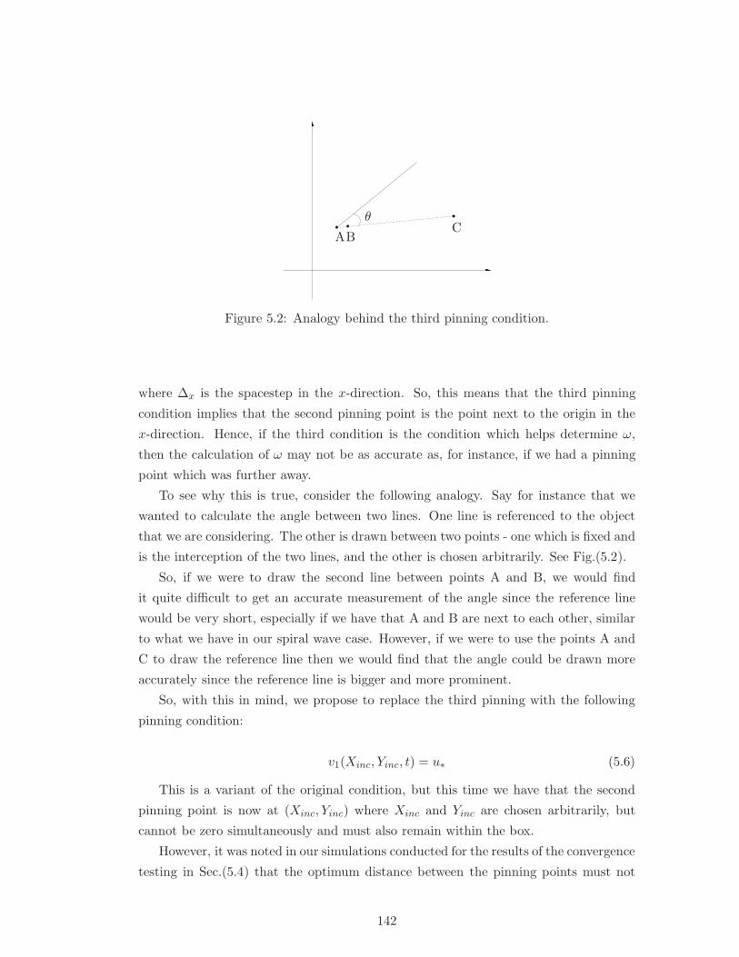
ABC
θ
Figure 5.2: Analogy behind the third pinning condition.
where ∆x is the spacestep in the x-direction. So, this means that the third pinning
condition implies that the second pinning point is the point next to the origin in the
x-direction. Hence, if the third condition is the condition which helps determine ω,
then the calculation of ω may not be as accurate as, for instance, if we had a pinning
point which was further away.
To see why this is true, consider the following analogy. Say for instance that we
wanted to calculate the angle between two lines. One line is referenced to the object
that we are considering. The other is drawn between two points - one which is fixed and
is the interception of the two lines, and the other is chosen arbitrarily. See Fig.(5.2).
So, if we were to draw the second line between points A and B, we would find
it quite difficult to get an accurate measurement of the angle since the reference line
would be very short, especially if we have that A and B are next to each other, similar
to what we have in our spiral wave case. However, if we were to use the points A and
C to draw the reference line then we would find that the angle could be drawn more
accurately since the reference line is bigger and more prominent.
So, with this in mind, we propose to replace the third pinning with the following
pinning condition:
v1(Xinc, Yinc, t) = u∗ (5.6)
This is a variant of the original condition, but this time we have that the second
pinning point is now at (Xinc, Yinc) where Xinc and Yinc are chosen arbitrarily, but
cannot be zero simultaneously and must also remain within the box.
However, it was noted in our simulations conducted for the results of the convergence
testing in Sec.(5.4) that the optimum distance between the pinning points must not
142
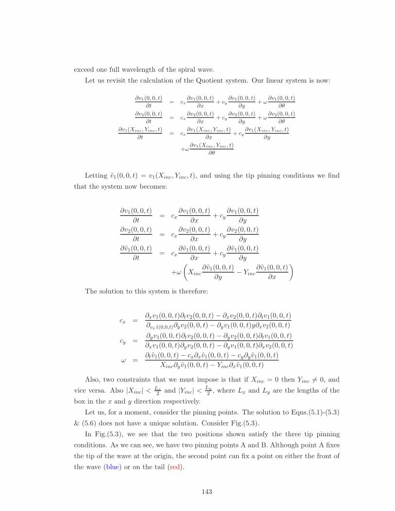
exceed one full wavelength of the spiral wave.
Let us revisit the calculation of the Quotient system. Our linear system is now:
∂v1(0, 0, t)
∂t= cx
∂v1(0, 0, t)
∂x+ cy
∂v1(0, 0, t)
∂y+ ω
∂v1(0, 0, t)
∂θ
∂v2(0, 0, t)
∂t= cx
∂v2(0, 0, t)
∂x+ cy
∂v2(0, 0, t)
∂y+ ω
∂v2(0, 0, t)
∂θ
∂v1(Xinc, Yinc, t)
∂t= cx
∂v1(Xinc, Yinc, t)
∂x+ cy
∂v1(Xinc, Yinc, t)
∂y
+ω∂v1(Xinc, Yinc, t)
∂θ
Letting v1(0, 0, t) = v1(Xinc, Yinc, t), and using the tip pinning conditions we find
that the system now becomes:
∂v1(0, 0, t)
∂t= cx
∂v1(0, 0, t)
∂x+ cy
∂v1(0, 0, t)
∂y
∂v2(0, 0, t)
∂t= cx
∂v2(0, 0, t)
∂x+ cy
∂v2(0, 0, t)
∂y
∂v1(0, 0, t)
∂t= cx
∂v1(0, 0, t)
∂x+ cy
∂v1(0, 0, t)
∂y
+ω
(
Xinc∂v1(0, 0, t)
∂y− Yinc
∂v1(0, 0, t)
∂x
)
The solution to this system is therefore:
cx =∂xv1(0, 0, t)∂tv2(0, 0, t) − ∂xv2(0, 0, t)∂tv1(0, 0, t)
∂vx1(0,0,t)∂yv2(0, 0, t) − ∂yv1(0, 0, t)y∂xv2(0, 0, t)
cy =∂yv1(0, 0, t)∂tv2(0, 0, t) − ∂yv2(0, 0, t)∂tv1(0, 0, t)
∂xv1(0, 0, t)∂yv2(0, 0, t) − ∂yv1(0, 0, t)∂xv2(0, 0, t)
ω =∂tv1(0, 0, t) − cx∂xv1(0, 0, t) − cy∂yv1(0, 0, t)
Xinc∂y v1(0, 0, t) − Yinc∂xv1(0, 0, t)
Also, two constraints that we must impose is that if Xinc = 0 then Yinc 6= 0, and
vice versa. Also |Xinc| < Lx
2 and |Yinc| < Ly
2 , where Lx and Ly are the lengths of the
box in the x and y direction respectively.
Let us, for a moment, consider the pinning points. The solution to Eqns.(5.1)-(5.3)
& (5.6) does not have a unique solution. Consider Fig.(5.3).
In Fig.(5.3), we see that the two positions shown satisfy the three tip pinning
conditions. As we can see, we have two pinning points A and B. Although point A fixes
the tip of the wave at the origin, the second point can fix a point on either the front of
the wave (blue) or on the tail (red).
143
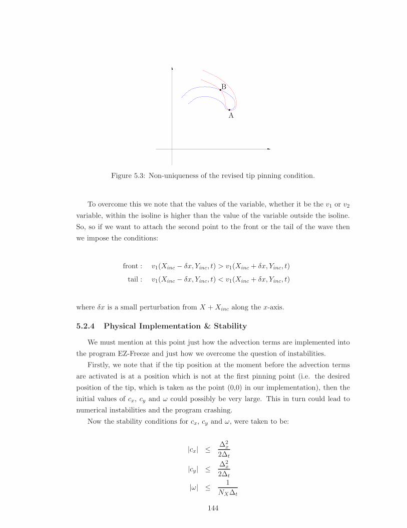
A
B
Figure 5.3: Non-uniqueness of the revised tip pinning condition.
To overcome this we note that the values of the variable, whether it be the v1 or v2
variable, within the isoline is higher than the value of the variable outside the isoline.
So, so if we want to attach the second point to the front or the tail of the wave then
we impose the conditions:
front : v1(Xinc − δx, Yinc, t) > v1(Xinc + δx, Yinc, t)
tail : v1(Xinc − δx, Yinc, t) < v1(Xinc + δx, Yinc, t)
where δx is a small perturbation from X + Xinc along the x-axis.
5.2.4 Physical Implementation & Stability
We must mention at this point just how the advection terms are implemented into
the program EZ-Freeze and just how we overcome the question of instabilities.
Firstly, we note that if the tip position at the moment before the advection terms
are activated is at a position which is not at the first pinning point (i.e. the desired
position of the tip, which is taken as the point (0,0) in our implementation), then the
initial values of cx, cy and ω could possibly be very large. This in turn could lead to
numerical instabilities and the program crashing.
Now the stability conditions for cx, cy and ω, were taken to be:
|cx| ≤∆2
x
2∆t
|cy| ≤∆2
x
2∆t
|ω| ≤ 1
NX∆t
144
where ∆x is the spacestep.
If the absolute values of cx and cy were greater than these limits then cx and cy
were restricted to the maximum (or minimum if cx or cy were negative) values stated
above. Also, we eliminated the need to restrict the values of cx and cy to their stability
limits by getting the program to physically move the spiral wave solution so that the
tip of the spiral wave is in the center of the box.
For ω, we implemented the restriction that if |ω| exceeded its maximum stability
value, then ω = 0. This lead to less instabilities occurring in the solutions.
5.2.5 Boundary Conditions
In EZ-Spiral, the user can specify either Neumann boundary conditions or periodic
boundary conditions. In EZ-Freeze, we use both Neumann boundary condition or
Dirichlet boundary condition. No periodic boundary conditions are used.
Numerically, Dirichlet boundary conditions can be translated as:
v
(
x,−Ly
2, t
)
= 0
v
(
x,Ly
2, t
)
= 0
v
(
−Lx
2, y, t
)
= 0
v
(
Lx
2, y, t
)
= 0
where Lx and Ly are the physical sizes of the boxes (remember that we take the center of
the box to be at the origin (0, 0)), and −Lx
2 ≤ x ≤ Lx
2 and −Ly
2 ≤ y ≤ Ly
2 . Numerically
we have:
v(i, 0, t) = 0
v(i,NY , t) = 0
v(0, j, t) = 0
v(NX , j, t) = 0
where v(i, j, t) is the numerically approximation to v(x, y, t), NX , NY are the number
of grid points in the numerical discretization, and i, j ∈ Z with 0 ≤ i ≤ NX and
0 ≤ j ≤ NY . We also assume that any point outside of the box (which we need for
spatial derivatives for both diffusion and advection) are automatically zero.
145
On the other hand, Neumann boundary condition are given as:
∂v
∂r= 0
which can be interpreted numerically as:
v(i,−1, t) = v(i, 1, t)
v(i,NY − 1, t) = v(i,NY + 1, t)
v(−1, j, t) = v(1, j, t)
v(NX − 1, j, t) = v(NX + 1, j, t)
where i, j ∈ Z with 0 ≤ i ≤ NX and 0 ≤ j ≤ NY .
When we come to use the second order scheme for spatial derivatives in the advection
terms, we also use the following additional scheme.
v(i,−2, t) = v(i, 2, t)
v(i,NY − 2, t) = v(i,NY + 2, t)
v(−2, j, t) = v(2, j, t)
v(NX − 2, j, t) = v(NX + 2, j, t)
5.2.6 The case for ǫ 6= 0.
We now describe when we have symmetry breaking perturbations within the sys-
tem. Throughout this project we are concerned with only three types of perturbations:
resonant drift (time dependent perturbations); Electrophoresis induced drift (rotational
breaking perturbations); and Inhomogeneity induced drift (parameters of the system
are dependent on the spatial coordinates).
In order to implement these three different types of drift into EZ-Freeze, we need
to consider the transformed perturbations, the derivation of which are given in Chap.3.
All perturbations are implemented into EZ-Freeze using the same technique. Again,
we use operator splitting and instead of having just two steps as we did for the case
when we had no perturbation (ǫ = 0), we now have three steps:
146
vn+ 1
3i,j = vn
i,j + ∆tR(vni,j) + O(∆2
t )
vn+ 2
3i,j = v
n+ 13
i,j + ∆tD(vn+ 1
3i,j ) + O(∆2
t )
vn+1i,j = v
n+ 23
i,j + ∆tA(vn+ 2
3i,j ) + O(∆2
t )
where, R are the Reaction-Diffusion terms, D are the perturbation terms, and A are
the advection terms.
We shall briefly consider each of the three examples individually.
Resonant Drift
When we have resonant drift, the perturbation is dependent only on time, not space.
Therefore, the transformed perturbation is exactly the same as the original perturba-
tion, since the transformation only concerns spatial transformations. Therefore, we
consider the perturbation as:
ǫh = A cos(Ωt + ξ)
where A is a vector whose elements are small (i.e. O(ǫ)), and is given by:
A = (A1, A2)T (5.7)
These parameters, like all the drift parameters used in these numerical simulations,
are specified within the file task.dat.
Electrophoresis Induced Drift
The transformed perturbation for this particular example is given by:
ǫh = B
(
cos(Θ)∂v0
∂x(r)− sin(Θ)
∂v0
∂y(r)
)
where B is a 2× 2 diagonalized matrix:
B =
(
B1 00 B2
)
The element B1 and B2 are both small quantities and are specified in the task.dat
file.
147
Inhomogeneity Induced Drift
Finally, the transformed perturbation for Inhomogeneity induced drift is give by:
ǫh = α1(X + x cos(Θ)− y sin(Θ))∂f
∂α(v0(r), α0)
where α1 is the drift gradient and controls the velocity of the drift.
5.2.7 Tip Reconstruction
We note that the coordinates for tip of the spiral wave are given:
dR
dt= ceiΘ
dΘ
dt= ω
We can solve these numerically using the following numerical scheme:
Θn+1 = Θn + ∆tωn
Xn+1 = Xn + ∆t(cx cos(Θn)− cy sin(Θn))
Y n+1 = Y n + ∆t(cx sin(Θn) + cy cos(Θn))
So, once we have found the cx, cy and ω, we can use these values to numerically
reconstruct the trajectory of the tip of the spiral wave as viewed in the laboratory frame
of reference.
5.3 Examples: Rigidly Rotation and Meander
In this section we shall show several examples. They will be split into two parts;
those for rigidly rotating spiral waves and those for meandering waves. We shall use
Barkley’s model for the rigid rotation and FHN for meander.
We shall show, for each example, results using a first order scheme, second order
scheme, Method 1 for calculating the quotient system, and also Method 2. We will also
show the values of the quotient system and how they converge for rigid rotation and
oscillate for meander. We shall also show the reconstructed tip trajectories.
For all simulations, we shall keep the following parameters fixed:
• Lx = Ly = 20
148
• Nx = Ny = 101
• ts = 0.1
where ts is the ratio of the timestep to the diffusion stability limit. Therefore, the
numerical parameters are:
• ∆x = 0.2
• ∆t = 0.001
5.3.1 Rigid Rotation
We use Barkley’s model in this particular example with the following model param-
eters being fixed throughout:
• a = 0.52
• b = 0.05
• ε = 0.02
Before we show these examples, we note that the trajectory in the laboratory frame of
reference is shown in Fig.(5.4)
We can also determine averaged values of the components of the quotient system, by
firstly using a Tikhonov Regularisation method and then solving the boundary value
problem with the Double Sweep Method. These are described in Sec.(2.4.2). The
results are shown in Fig.(5.4), with the original data shown in the top left hand corner
of the figure.
We can see the values of cx , cy and ω do not converge to one particular value but
oscillate with a period that is equal to the period of the spiral wave. This suggests
that these small oscillations are due to either the influence of the boundaries or the
discretization of the numerical methods. However, we note that the averaged values
are cx = 0.796796, cy = −0.7931725 and ω = −0.916312. However, we must note that
the values of cx and cy are distorted by the regularisation technique for high values of
λ (regularization parameter), but ω is not distorted .
This information is useful just to get an idea of what the quotient solution should
look like. It is by no means a highly accurate calculation of the quotient solution. It is
a means to depress the noise in the numerical data so that it can be differentiated.
We shown in Figs(5.5)-(5.8) the results from the simulations using first and second
order scheme for method 1 and a first and second order for method two. We can see
that each of the four simulations produce different results, and we show in table (5.3.1)
the values of the components of the quotient solution.
149
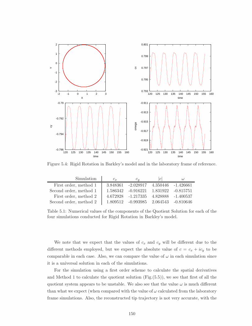
-3
-2
-1
0
1
2
-2 -1 0 1 2 3
Y
X
0.793
0.795
0.797
0.799
0.801
120 125 130 135 140 145 150 155 160
cx
time
-0.796
-0.794
-0.792
-0.79
120 125 130 135 140 145 150 155 160
cy
time
-0.921
-0.919
-0.917
-0.915
-0.913
-0.911
120 125 130 135 140 145 150 155 160
omeg
a
time
Figure 5.4: Rigid Rotation in Barkley’s model and in the laboratory frame of reference.
Simulation cx cy |c| ω
First order, method 1 3.848361 -2.028917 4.350446 -1.426661Second order, method 1 1.586342 -0.916221 1.831922 -0.815751
First order, method 2 4.672928 -1.217335 4.828888 -1.400537Second order, method 2 1.809512 -0.993985 2.064543 -0.810646
Table 5.1: Numerical values of the components of the Quotient Solution for each of thefour simulations conducted for Rigid Rotation in Barkley’s model.
We note that we expect that the values of cx and cy will be different due to the
different methods employed, but we expect the absolute value of c = cx + icy to be
comparable in each case. Also, we can compare the value of ω in each simulation since
it is a universal solution in each of the simulations.
For the simulation using a first order scheme to calculate the spatial derivatives
and Method 1 to calculate the quotient solution (Fig.(5.5)), we see that first of all the
quotient system appears to be unstable. We also see that the value ω is much different
than what we expect (when compared with the value of ω calculated from the laboratory
frame simulations. Also, the reconstructed tip trajectory is not very accurate, with the
150
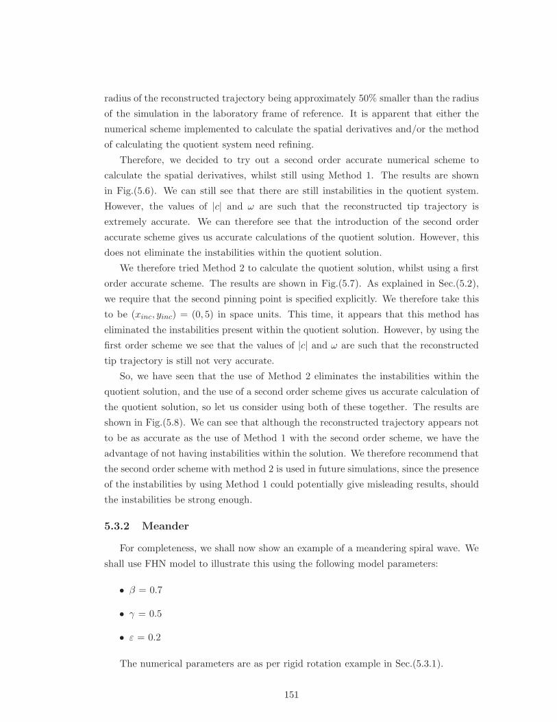
radius of the reconstructed trajectory being approximately 50% smaller than the radius
of the simulation in the laboratory frame of reference. It is apparent that either the
numerical scheme implemented to calculate the spatial derivatives and/or the method
of calculating the quotient system need refining.
Therefore, we decided to try out a second order accurate numerical scheme to
calculate the spatial derivatives, whilst still using Method 1. The results are shown
in Fig.(5.6). We can still see that there are still instabilities in the quotient system.
However, the values of |c| and ω are such that the reconstructed tip trajectory is
extremely accurate. We can therefore see that the introduction of the second order
accurate scheme gives us accurate calculations of the quotient solution. However, this
does not eliminate the instabilities within the quotient solution.
We therefore tried Method 2 to calculate the quotient solution, whilst using a first
order accurate scheme. The results are shown in Fig.(5.7). As explained in Sec.(5.2),
we require that the second pinning point is specified explicitly. We therefore take this
to be (xinc, yinc) = (0, 5) in space units. This time, it appears that this method has
eliminated the instabilities present within the quotient solution. However, by using the
first order scheme we see that the values of |c| and ω are such that the reconstructed
tip trajectory is still not very accurate.
So, we have seen that the use of Method 2 eliminates the instabilities within the
quotient solution, and the use of a second order scheme gives us accurate calculation of
the quotient solution, so let us consider using both of these together. The results are
shown in Fig.(5.8). We can see that although the reconstructed trajectory appears not
to be as accurate as the use of Method 1 with the second order scheme, we have the
advantage of not having instabilities within the solution. We therefore recommend that
the second order scheme with method 2 is used in future simulations, since the presence
of the instabilities by using Method 1 could potentially give misleading results, should
the instabilities be strong enough.
5.3.2 Meander
For completeness, we shall now show an example of a meandering spiral wave. We
shall use FHN model to illustrate this using the following model parameters:
• β = 0.7
• γ = 0.5
• ε = 0.2
The numerical parameters are as per rigid rotation example in Sec.(5.3.1).
151
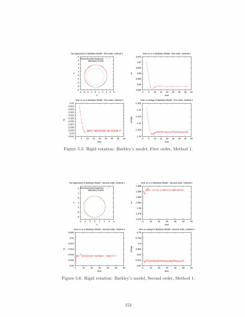
-4
-3
-2
-1
0
1
2
3
4
5
-4 -3 -2 -1 0 1 2 3 4 5
Y
X
Tip trajectories in Barkleys Model - first order, method 1
Reconstructed trajectorylaboratory frame
3.845
3.85
3.855
3.86
3.865
3.87
3.875
0 5 10 15 20 25 30 35 40
cx
time
time vs cx in Barkleys Model - first order, method 1
-2.031-2.03
-2.029-2.028-2.027-2.026-2.025-2.024-2.023-2.022-2.021-2.02
0 5 10 15 20 25 30 35 40
cy
time
time vs cy in Barkleys Model - first order, method 1
-1.43
-1.425
-1.42
-1.415
-1.41
-1.405
0 5 10 15 20 25 30 35 40
omeg
a
time
time vs omega in Barkleys Model - first order, method 1
Figure 5.5: Rigid rotation: Barkley’s model, First order, Method 1.
-4
-3
-2
-1
0
1
2
-3 -2 -1 0 1 2 3 4
Y
X
Tip trajectories in Barkleys Model - second order, method 1
Reconstructed trajectorylaboratory frame
1.576
1.578
1.58
1.582
1.584
1.586
1.588
0 10 20 30 40 50 60
cx
time
time vs cx in Barkleys Model - second order, method 1
-0.92
-0.918
-0.916
-0.914
-0.912
-0.91
-0.908
0 10 20 30 40 50 60
cy
time
time vs cy in Barkleys Model - second order, method 1
-0.82
-0.815
-0.81
-0.805
-0.8
-0.795
-0.79
0 10 20 30 40 50 60
omeg
a
time
time vs omega in Barkleys Model - second order, method 1
Figure 5.6: Rigid rotation: Barkley’s model, Second order, Method 1.
152
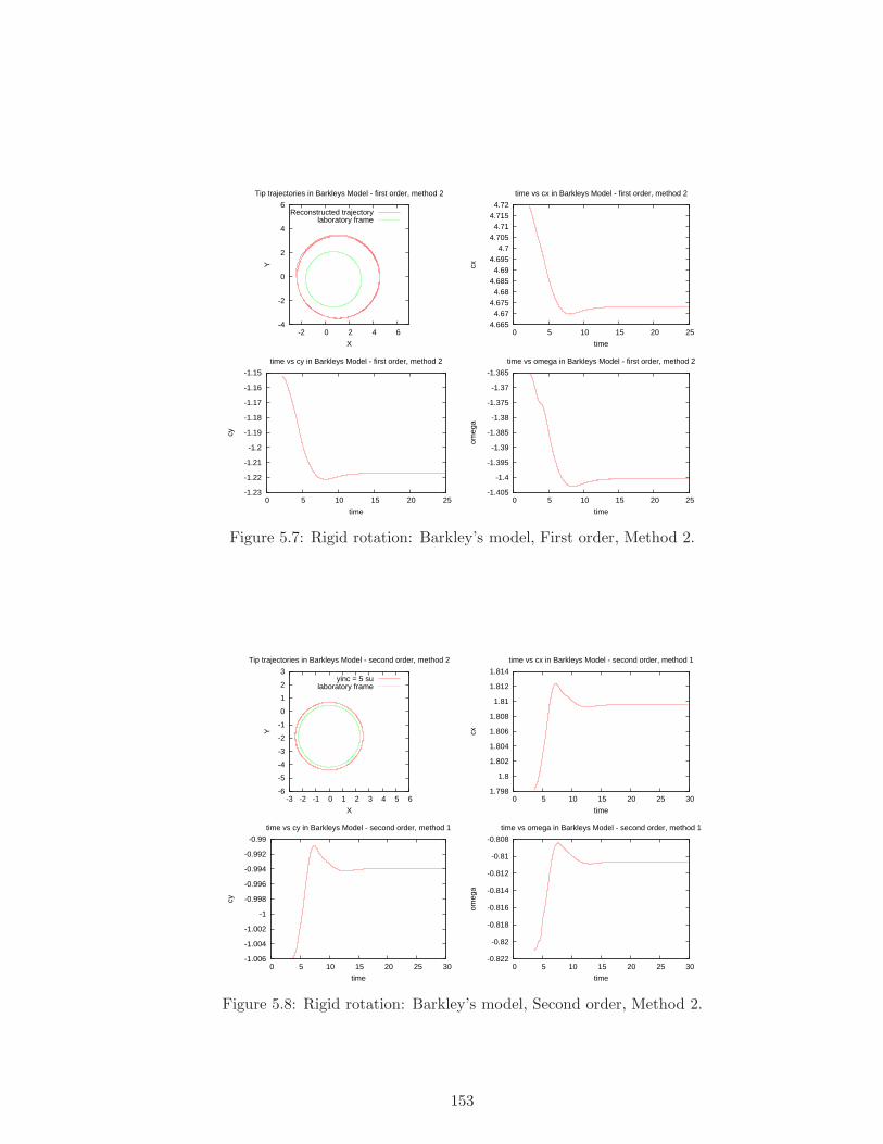
-4
-2
0
2
4
6
-2 0 2 4 6
Y
X
Tip trajectories in Barkleys Model - first order, method 2
Reconstructed trajectorylaboratory frame
4.665 4.67
4.675 4.68
4.685 4.69
4.695 4.7
4.705 4.71
4.715 4.72
0 5 10 15 20 25
cx
time
time vs cx in Barkleys Model - first order, method 2
-1.23
-1.22
-1.21
-1.2
-1.19
-1.18
-1.17
-1.16
-1.15
0 5 10 15 20 25
cy
time
time vs cy in Barkleys Model - first order, method 2
-1.405
-1.4
-1.395
-1.39
-1.385
-1.38
-1.375
-1.37
-1.365
0 5 10 15 20 25
omeg
a
time
time vs omega in Barkleys Model - first order, method 2
Figure 5.7: Rigid rotation: Barkley’s model, First order, Method 2.
-6
-5
-4
-3
-2
-1
0
1
2
3
-3 -2 -1 0 1 2 3 4 5 6
Y
X
Tip trajectories in Barkleys Model - second order, method 2
yinc = 5 sulaboratory frame
1.798
1.8
1.802
1.804
1.806
1.808
1.81
1.812
1.814
0 5 10 15 20 25 30
cx
time
time vs cx in Barkleys Model - second order, method 1
-1.006
-1.004
-1.002
-1
-0.998
-0.996
-0.994
-0.992
-0.99
0 5 10 15 20 25 30
cy
time
time vs cy in Barkleys Model - second order, method 1
-0.822
-0.82
-0.818
-0.816
-0.814
-0.812
-0.81
-0.808
0 5 10 15 20 25 30
omeg
a
time
time vs omega in Barkleys Model - second order, method 1
Figure 5.8: Rigid rotation: Barkley’s model, Second order, Method 2.
153
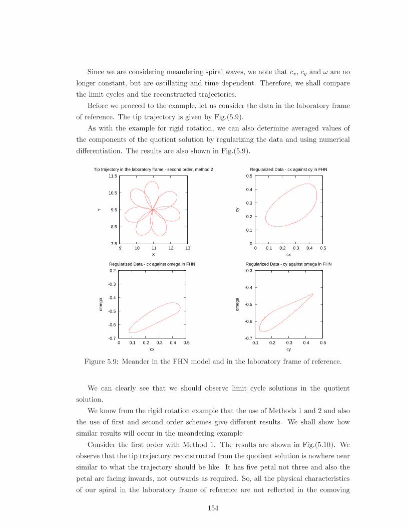
Since we are considering meandering spiral waves, we note that cx, cy and ω are no
longer constant, but are oscillating and time dependent. Therefore, we shall compare
the limit cycles and the reconstructed trajectories.
Before we proceed to the example, let us consider the data in the laboratory frame
of reference. The tip trajectory is given by Fig.(5.9).
As with the example for rigid rotation, we can also determine averaged values of
the components of the quotient solution by regularizing the data and using numerical
differentiation. The results are also shown in Fig.(5.9).
7.5
8.5
9.5
10.5
11.5
9 10 11 12 13
Y
X
Tip trajectory in the laboratory frame - second order, method 2
0
0.1
0.2
0.3
0.4
0.5
0 0.1 0.2 0.3 0.4 0.5
cy
cx
Regularized Data - cx against cy in FHN
-0.7
-0.6
-0.5
-0.4
-0.3
-0.2
0 0.1 0.2 0.3 0.4 0.5
omeg
a
cx
Regularized Data - cx against omega in FHN
-0.7
-0.6
-0.5
-0.4
-0.3
0.1 0.2 0.3 0.4 0.5
omeg
a
cy
Regularized Data - cy against omega in FHN
Figure 5.9: Meander in the FHN model and in the laboratory frame of reference.
We can clearly see that we should observe limit cycle solutions in the quotient
solution.
We know from the rigid rotation example that the use of Methods 1 and 2 and also
the use of first and second order schemes give different results. We shall show how
similar results will occur in the meandering example
Consider the first order with Method 1. The results are shown in Fig.(5.10). We
observe that the tip trajectory reconstructed from the quotient solution is nowhere near
similar to what the trajectory should be like. It has five petal not three and also the
petal are facing inwards, not outwards as required. So, all the physical characteristics
of our spiral in the laboratory frame of reference are not reflected in the comoving
154
frame of reference when we reconstructed the tip. However, what is not quite evident
here is that there are “wobbles” in the quotient solution. The quotient solution must
not be calculated properly and to an acceptable level of accuracy due to the fact that
the reconstructed trajectory is nothing similar to what it should be.
Now consider introducing the second order scheme whilst retaining Method 1,
Fig.(5.11). We now see that the anomalies in the quotient are very much evident,
so much so that we have plotted the data using just points and not lines, since the
plots would be unreadable otherwise. So, we also notice that the trajectory is very
much like what we want. As expected, the quotient data has wobbles but we get an
accurately calculated tip trajectory.
Let us now use a first order scheme but this time with Method 2, Fig.(5.12). We
observe that although there are now no instabilities in the quotient solution, the quo-
tient solution is not very accurate due to the tip trajectory being nothing like what it
should.
Therefore, we use a second order scheme with Method 2, Fig.(5.13). As expected,
this gives an accurately calculated tip trajectory.
155
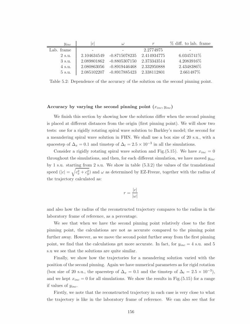
yinc |c| ω r % diff. to lab. frame
Lab. frame - - 2.2774975 -2 s.u. 2.104634549 -0.8715078235 2.414934775 6.0345741%3 s.u. 2.089801862 -0.8805307150 2.373343514 4.2083916%4 s.u. 2.080863056 -0.8919446468 2.332950888 2.4348386%5 s.u. 2.085102207 -0.8917885423 2.338112801 2.661487%
Table 5.2: Dependence of the accuracy of the solution on the second pinning point.
Accuracy by varying the second pinning point (xinc, yinc)
We finish this section by showing how the solutions differ when the second pinning
is placed at different distances from the origin (first pinning point). We will show two
tests: one for a rigidly rotating spiral wave solution to Barkley’s model; the second for
a meandering spiral wave solution in FHN. We shall use a box size of 20 s.u., with a
spacestep of ∆x = 0.1 and timstep of ∆t = 2.5× 10⁻³ in all the simulations.
Consider a rigidly rotating spiral wave solution and Fig.(5.15). We have xinc = 0
throughout the simulations, and then, for each different simulation, we have moved yinc
by 1 s.u. starting from 2 s.u. We show in table (5.3.2) the values of the translational
speed (|c| =√
c2x + c2
y) and ω as determined by EZ-Freeze, together with the radius of
the trajectory calculated as:
r =|c||ω|
and also how the radius of the reconstructed trajectory compares to the radius in the
laboratory frame of reference, as a percentage.
We see that when we have the second pinning point relatively close to the first
pinning point, the calculations are not as accurate compared to the pinning point
further away. However, as we move the second point further away from the first pinning
point, we find that the calculations get more accurate. In fact, for yinc = 4 s.u. and 5
s.u we see that the solutions are quite similar.
Finally, we show how the trajectories for a meandering solution varied with the
position of the second pinning. Again we have numerical parameters as for rigid rotation
(box size of 20 s.u., the spacestep of ∆x = 0.1 and the timstep of ∆t = 2.5 × 10⁻³),
and we kept xinc = 0 for all simulations. We show the results in Fig.(5.15) for a range
if values of yinc.
Firstly, we note that the reconstructed trajectory in each case is very close to what
the trajectory is like in the laboratory frame of reference. We can also see that for
156
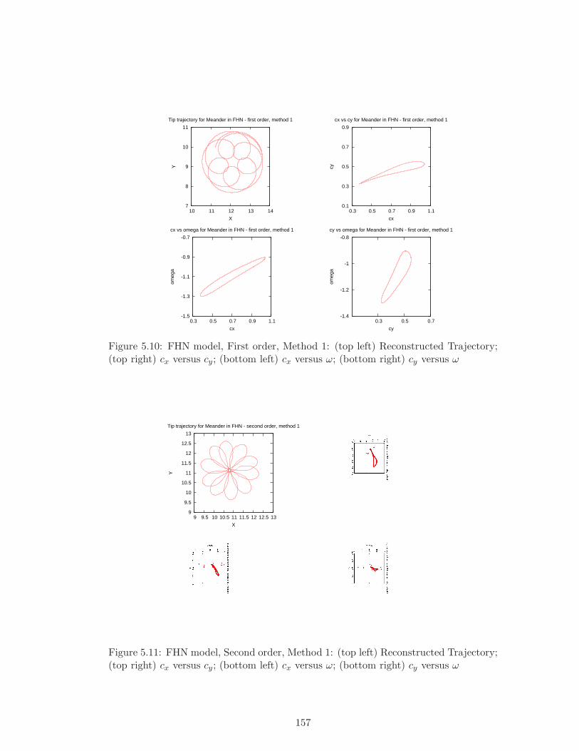
7
8
9
10
11
10 11 12 13 14
Y
X
Tip trajectory for Meander in FHN - first order, method 1
0.1
0.3
0.5
0.7
0.9
0.3 0.5 0.7 0.9 1.1
cy
cx
cx vs cy for Meander in FHN - first order, method 1
-1.5
-1.3
-1.1
-0.9
-0.7
0.3 0.5 0.7 0.9 1.1
omeg
a
cx
cx vs omega for Meander in FHN - first order, method 1
-1.4
-1.2
-1
-0.8
0.3 0.5 0.7
omeg
acy
cy vs omega for Meander in FHN - first order, method 1
Figure 5.10: FHN model, First order, Method 1: (top left) Reconstructed Trajectory;(top right) cx versus cy; (bottom left) cx versus ω; (bottom right) cy versus ω
9
9.5
10
10.5
11
11.5
12
12.5
13
9 9.5 10 10.5 11 11.5 12 12.5 13
Y
X
Tip trajectory for Meander in FHN - second order, method 1
Figure 5.11: FHN model, Second order, Method 1: (top left) Reconstructed Trajectory;(top right) cx versus cy; (bottom left) cx versus ω; (bottom right) cy versus ω
157
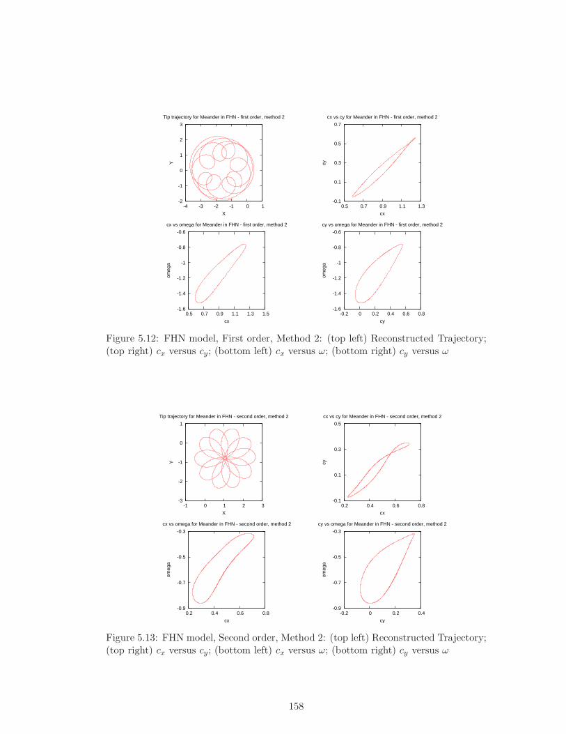
-2
-1
0
1
2
3
-4 -3 -2 -1 0 1
Y
X
Tip trajectory for Meander in FHN - first order, method 2
-0.1
0.1
0.3
0.5
0.7
0.5 0.7 0.9 1.1 1.3
cy
cx
cx vs cy for Meander in FHN - first order, method 2
-1.6
-1.4
-1.2
-1
-0.8
-0.6
0.5 0.7 0.9 1.1 1.3 1.5
omeg
a
cx
cx vs omega for Meander in FHN - first order, method 2
-1.6
-1.4
-1.2
-1
-0.8
-0.6
-0.2 0 0.2 0.4 0.6 0.8
omeg
acy
cy vs omega for Meander in FHN - first order, method 2
Figure 5.12: FHN model, First order, Method 2: (top left) Reconstructed Trajectory;(top right) cx versus cy; (bottom left) cx versus ω; (bottom right) cy versus ω
-3
-2
-1
0
1
-1 0 1 2 3
Y
X
Tip trajectory for Meander in FHN - second order, method 2
-0.1
0.1
0.3
0.5
0.2 0.4 0.6 0.8
cy
cx
cx vs cy for Meander in FHN - second order, method 2
-0.9
-0.7
-0.5
-0.3
0.2 0.4 0.6 0.8
omeg
a
cx
cx vs omega for Meander in FHN - second order, method 2
-0.9
-0.7
-0.5
-0.3
-0.2 0 0.2 0.4
omeg
a
cy
cy vs omega for Meander in FHN - second order, method 2
Figure 5.13: FHN model, Second order, Method 2: (top left) Reconstructed Trajectory;(top right) cx versus cy; (bottom left) cx versus ω; (bottom right) cy versus ω
158
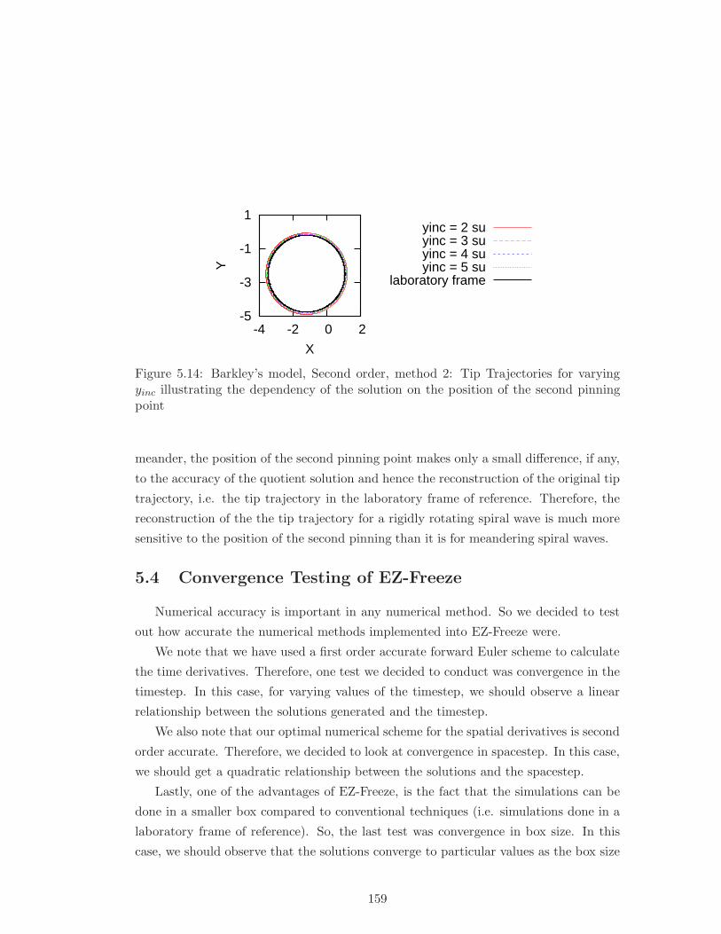
-5
-3
-1
1
-4 -2 0 2
Y
X
yinc = 2 suyinc = 3 suyinc = 4 suyinc = 5 su
laboratory frame
Figure 5.14: Barkley’s model, Second order, method 2: Tip Trajectories for varyingyinc illustrating the dependency of the solution on the position of the second pinningpoint
meander, the position of the second pinning point makes only a small difference, if any,
to the accuracy of the quotient solution and hence the reconstruction of the original tip
trajectory, i.e. the tip trajectory in the laboratory frame of reference. Therefore, the
reconstruction of the the tip trajectory for a rigidly rotating spiral wave is much more
sensitive to the position of the second pinning than it is for meandering spiral waves.
5.4 Convergence Testing of EZ-Freeze
Numerical accuracy is important in any numerical method. So we decided to test
out how accurate the numerical methods implemented into EZ-Freeze were.
We note that we have used a first order accurate forward Euler scheme to calculate
the time derivatives. Therefore, one test we decided to conduct was convergence in the
timestep. In this case, for varying values of the timestep, we should observe a linear
relationship between the solutions generated and the timestep.
We also note that our optimal numerical scheme for the spatial derivatives is second
order accurate. Therefore, we decided to look at convergence in spacestep. In this case,
we should get a quadratic relationship between the solutions and the spacestep.
Lastly, one of the advantages of EZ-Freeze, is the fact that the simulations can be
done in a smaller box compared to conventional techniques (i.e. simulations done in a
laboratory frame of reference). So, the last test was convergence in box size. In this
case, we should observe that the solutions converge to particular values as the box size
159
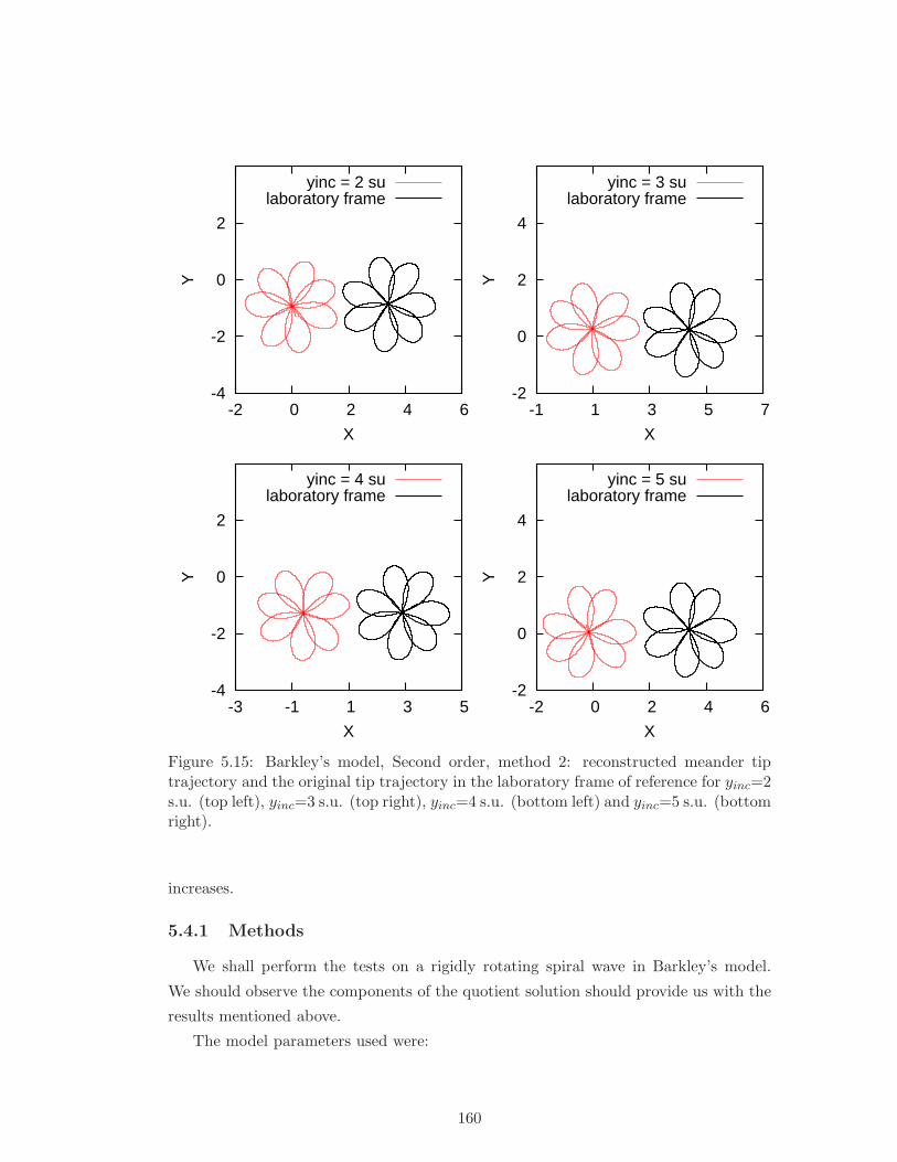
-4
-2
0
2
-2 0 2 4 6
Y
X
yinc = 2 sulaboratory frame
-2
0
2
4
-1 1 3 5 7
Y
X
yinc = 3 sulaboratory frame
-4
-2
0
2
-3 -1 1 3 5
Y
X
yinc = 4 sulaboratory frame
-2
0
2
4
-2 0 2 4 6
Y
X
yinc = 5 sulaboratory frame
Figure 5.15: Barkley’s model, Second order, method 2: reconstructed meander tiptrajectory and the original tip trajectory in the laboratory frame of reference for yinc=2s.u. (top left), yinc=3 s.u. (top right), yinc=4 s.u. (bottom left) and yinc=5 s.u. (bottomright).
increases.
5.4.1 Methods
We shall perform the tests on a rigidly rotating spiral wave in Barkley’s model.
We should observe the components of the quotient solution should provide us with the
results mentioned above.
The model parameters used were:
160
a = 0.52
b = 0.05
ε = 0.02
We also state below the “best” numerical and physical parameters that we used
throughout the tests:
∆t = 1.11 × 10⁻⁴
∆x = 115
Box Size LX = 60s.u.
We also note that the timestep is controlled in EZ-Freeze by a parameter called ts,
which is the ratio of the timestep to the diffusion stability limit. This optimal timestep
corresponds to ts = 0.1. The timestep is given by the formula:
∆t =ts∆
2x
4(5.8)
Also, we have that we must have a grid size of NX = 901 for a spacestep of ∆x = 115 .
In the convergence test for the timestep, ∆t, we kept LX and ∆x at the optimal
values, and varied the timestep by adjusting the parameter ts. Starting at the optimal
value, we increased ts in steps of 0.04 each time, until the solution became unstable.
For convergence in the box size size, we kept the ∆t and ∆x at the optimal values,
and varied the box size by starting at the optimal value reduced the box size by 5 s.u.
each time, until we got to LX = 15. After this we decreased the box size in steps of 1
s.u. The reason for this will become apparent in the results section.
For the convergence in the spacestep, ∆x, we must mention at this point the impor-
tance of the pinning points. We came across several problems with the testing and one
of these problems was tied down to the position of the second tip pinning condition.
We noted in Sec.(5.2) that the second pinning point could vastly improve the accuracy
of the calculation of the quotient system, in particular, ω. When we first conducted
the tests we set the second point at (xinc, yinc) = (0, 2) in space units. As we found
out, the position of the second pinning point is too close to the first and therefore the
results generated were not very clear. Therefore, we decided to put the second pinning
point further away from the first. In fact we tried to put it near one of the boundaries,
keeping xinc = 0 and setting yinc = LX2 − 1, i.e. 1 s.u. away from the boundary. Un-
fortunately, this yielded rather strange and, what we conceived, as inaccurate results.
One of the reasons for this that is conjected by the author is that the distance between
the pinning points is more than the wavelength of the spiral. Therefore, in the tests
161
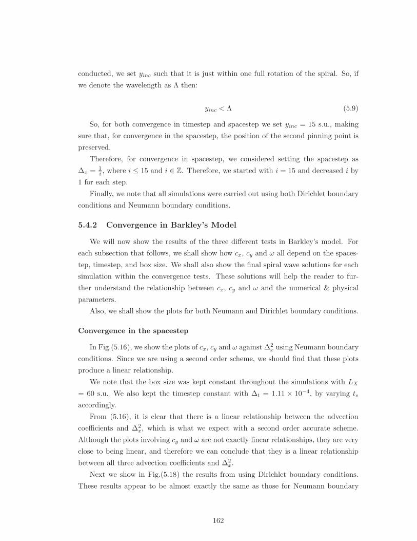
conducted, we set yinc such that it is just within one full rotation of the spiral. So, if
we denote the wavelength as Λ then:
yinc < Λ (5.9)
So, for both convergence in timestep and spacestep we set yinc = 15 s.u., making
sure that, for convergence in the spacestep, the position of the second pinning point is
preserved.
Therefore, for convergence in spacestep, we considered setting the spacestep as
∆x = 1i, where i ≤ 15 and i ∈ Z. Therefore, we started with i = 15 and decreased i by
1 for each step.
Finally, we note that all simulations were carried out using both Dirichlet boundary
conditions and Neumann boundary conditions.
5.4.2 Convergence in Barkley’s Model
We will now show the results of the three different tests in Barkley’s model. For
each subsection that follows, we shall show how cx, cy and ω all depend on the spaces-
tep, timestep, and box size. We shall also show the final spiral wave solutions for each
simulation within the convergence tests. These solutions will help the reader to fur-
ther understand the relationship between cx, cy and ω and the numerical & physical
parameters.
Also, we shall show the plots for both Neumann and Dirichlet boundary conditions.
Convergence in the spacestep
In Fig.(5.16), we show the plots of cx, cy and ω against ∆2x using Neumann boundary
conditions. Since we are using a second order scheme, we should find that these plots
produce a linear relationship.
We note that the box size was kept constant throughout the simulations with LX
= 60 s.u. We also kept the timestep constant with ∆t = 1.11 × 10⁻⁴, by varying ts
accordingly.
From (5.16), it is clear that there is a linear relationship between the advection
coefficients and ∆2x, which is what we expect with a second order accurate scheme.
Although the plots involving cy and ω are not exactly linear relationships, they are very
close to being linear, and therefore we can conclude that they is a linear relationship
between all three advection coefficients and ∆2x.
Next we show in Fig.(5.18) the results from using Dirichlet boundary conditions.
These results appear to be almost exactly the same as those for Neumann boundary
162
conditions. So we can conclude that the choice of boundary conditions is irrelevant in
these tests since both give the same results.
We also show the final solutions in Figs.(5.17) and (5.19).
163
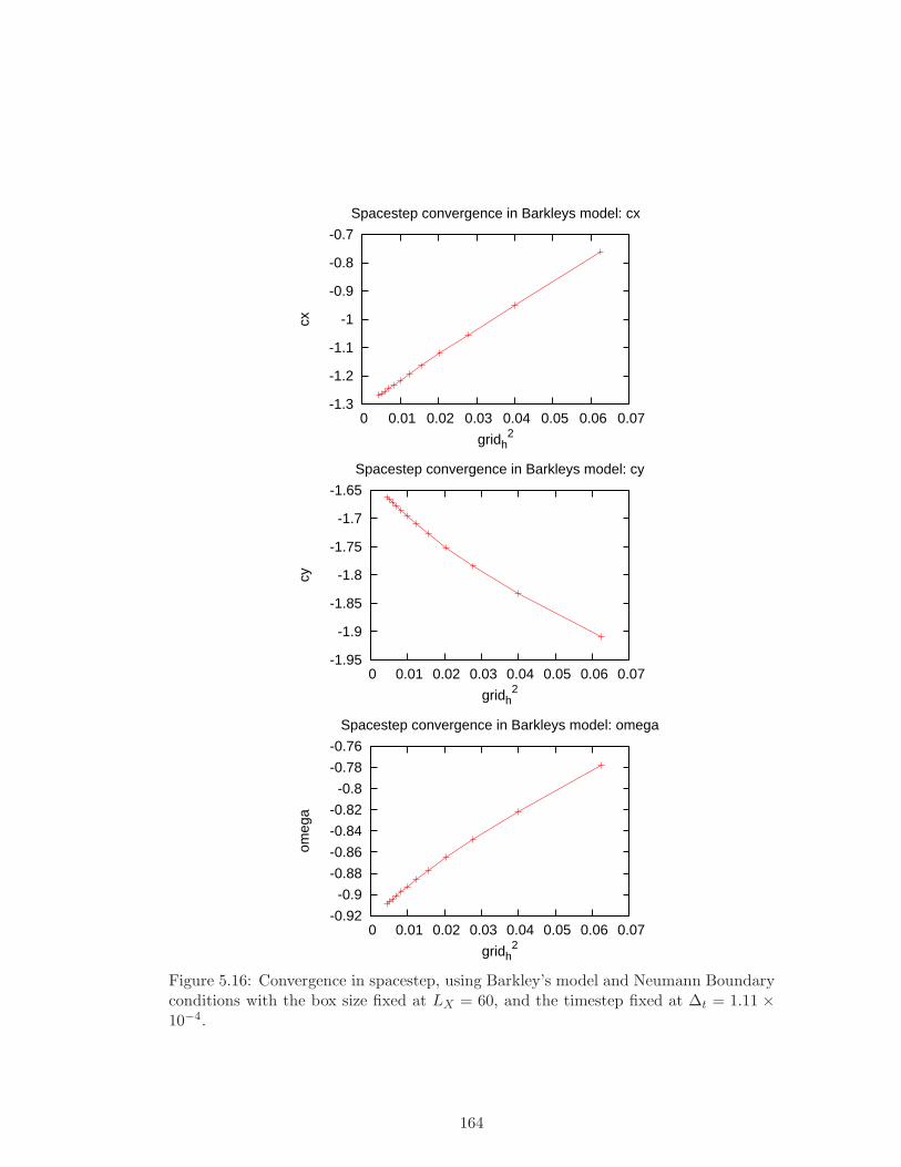
-1.3
-1.2
-1.1
-1
-0.9
-0.8
-0.7
0 0.01 0.02 0.03 0.04 0.05 0.06 0.07
cx
gridh2
Spacestep convergence in Barkleys model: cx
-1.95
-1.9
-1.85
-1.8
-1.75
-1.7
-1.65
0 0.01 0.02 0.03 0.04 0.05 0.06 0.07
cy
gridh2
Spacestep convergence in Barkleys model: cy
-0.92
-0.9
-0.88
-0.86
-0.84
-0.82
-0.8
-0.78
-0.76
0 0.01 0.02 0.03 0.04 0.05 0.06 0.07
omeg
a
gridh2
Spacestep convergence in Barkleys model: omega
Figure 5.16: Convergence in spacestep, using Barkley’s model and Neumann Boundaryconditions with the box size fixed at LX = 60, and the timestep fixed at ∆t = 1.11 ×10⁻⁴.
164
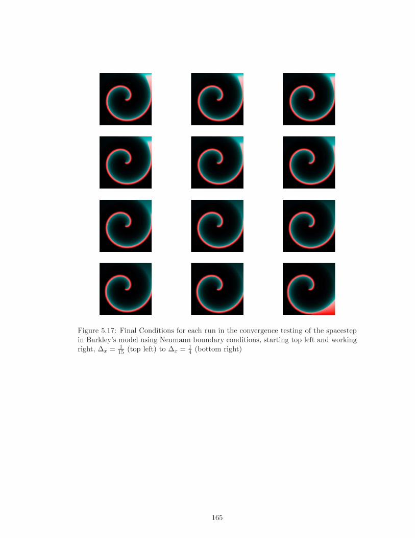
Figure 5.17: Final Conditions for each run in the convergence testing of the spacestepin Barkley’s model using Neumann boundary conditions, starting top left and workingright, ∆x = 1
15 (top left) to ∆x = 14 (bottom right)
165
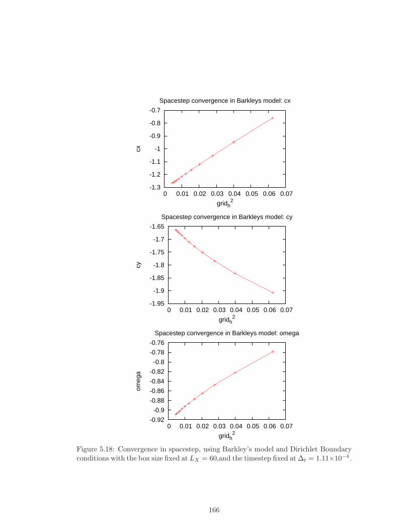
-1.3
-1.2
-1.1
-1
-0.9
-0.8
-0.7
0 0.01 0.02 0.03 0.04 0.05 0.06 0.07
cx
gridh2
Spacestep convergence in Barkleys model: cx
-1.95
-1.9
-1.85
-1.8
-1.75
-1.7
-1.65
0 0.01 0.02 0.03 0.04 0.05 0.06 0.07
cy
gridh2
Spacestep convergence in Barkleys model: cy
-0.92
-0.9
-0.88
-0.86
-0.84
-0.82
-0.8
-0.78
-0.76
0 0.01 0.02 0.03 0.04 0.05 0.06 0.07
omeg
a
gridh2
Spacestep convergence in Barkleys model: omega
Figure 5.18: Convergence in spacestep, using Barkley’s model and Dirichlet Boundaryconditions with the box size fixed at LX = 60,and the timestep fixed at ∆t = 1.11×10⁻⁴.
166
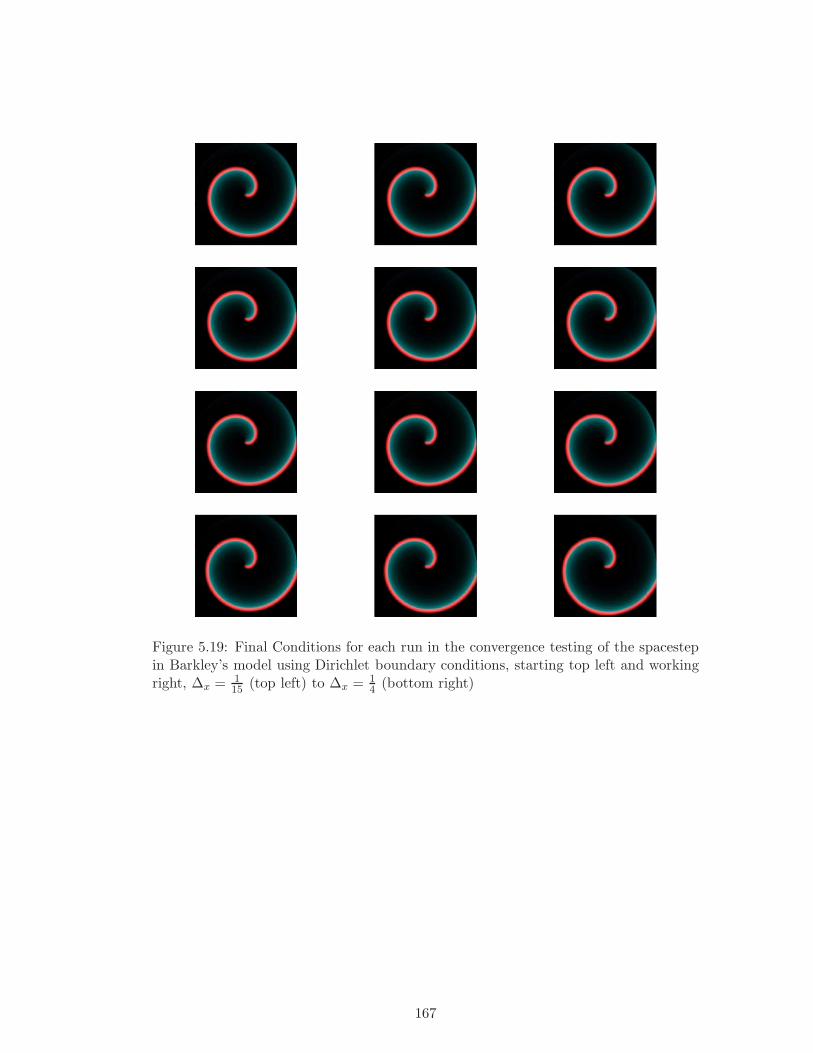
Figure 5.19: Final Conditions for each run in the convergence testing of the spacestepin Barkley’s model using Dirichlet boundary conditions, starting top left and workingright, ∆x = 1
15 (top left) to ∆x = 14 (bottom right)
167
Convergence in the box size
We will now show how cx, cy and ω depend on the size of the box. In this instance,
we should observe that after a particular size of box, the advection coefficients settle
down to a fixed value.
Also, we kept the following numerical parameters constant throughout the simula-
tions:
• spacestep, ∆x = 115
• timestep, ∆t = 1.1× 10⁻³ (with ts = 0.1)
Starting from a box size of 60 s.u., we ran a number of simulations with each
consecutive simulation have a box size 5 s.u. less than the previous.
In Fig.(5.20) we show the results using Neumann boundary conditions. It is clearly
evident that in the plots of cx and cy against the box size, we get that the values of
cx and cy settle down to a fixed value, give or take some very small oscillations of the
order of 1.0 × 10⁻⁴. In the plot of ω against the box, it appears that there are some
significant oscillations, but again, these oscillations are only of the order 1.0× 10⁻⁴.
We also show in Fig.(5.22) the same plots but this time using Dirichlet boundary
conditions. As we can see, we get almost exactly the same results. The values of cx,
cy and ω all seem to settle down to the same values as those using Neumann boundary
conditions.
We also show the spiral wave solutions for each of the simulations within the tests
in Figs.(5.21) and (5.23).
168
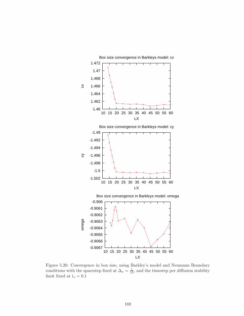
1.46
1.462
1.464
1.466
1.468
1.47
1.472
10 15 20 25 30 35 40 45 50 55 60
cx
LX
Box size convergence in Barkleys model: cx
-1.502
-1.5
-1.498
-1.496
-1.494
-1.492
-1.49
10 15 20 25 30 35 40 45 50 55 60
cy
LX
Box size convergence in Barkleys model: cy
-0.9067
-0.9066
-0.9065
-0.9064
-0.9063
-0.9062
-0.9061
-0.906
10 15 20 25 30 35 40 45 50 55 60
omeg
a
LX
Box size convergence in Barkleys model: omega
Figure 5.20: Convergence in box size, using Barkley’s model and Neumann Boundaryconditions with the spacestep fixed at ∆x = 1
15 , and the timestep per diffusion stabilitylimit fixed at ts = 0.1
169
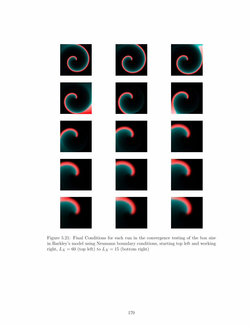
Figure 5.21: Final Conditions for each run in the convergence testing of the box sizein Barkley’s model using Neumann boundary conditions, starting top left and workingright, LX = 60 (top left) to LX = 15 (bottom right)
170
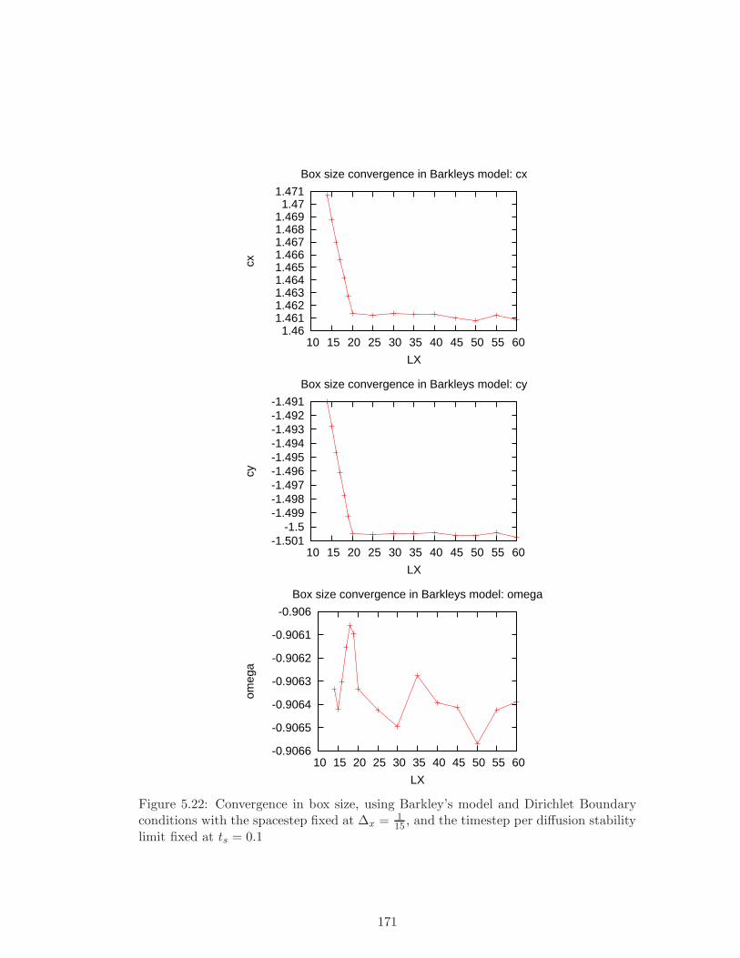
1.46 1.461 1.462 1.463 1.464 1.465 1.466 1.467 1.468 1.469
1.47 1.471
10 15 20 25 30 35 40 45 50 55 60
cx
LX
Box size convergence in Barkleys model: cx
-1.501-1.5
-1.499-1.498-1.497-1.496-1.495-1.494-1.493-1.492-1.491
10 15 20 25 30 35 40 45 50 55 60
cy
LX
Box size convergence in Barkleys model: cy
-0.9066
-0.9065
-0.9064
-0.9063
-0.9062
-0.9061
-0.906
10 15 20 25 30 35 40 45 50 55 60
omeg
a
LX
Box size convergence in Barkleys model: omega
Figure 5.22: Convergence in box size, using Barkley’s model and Dirichlet Boundaryconditions with the spacestep fixed at ∆x = 1
15 , and the timestep per diffusion stabilitylimit fixed at ts = 0.1
171
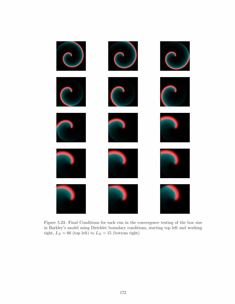
Figure 5.23: Final Conditions for each run in the convergence testing of the box sizein Barkley’s model using Dirichlet boundary conditions, starting top left and workingright, LX = 60 (top left) to LX = 15 (bottom right)
172
Convergence in the timestep
Finally for Barkley’s model, we consider the convergence in the timestep. The
results for Neumann boundary conditions are shown in Fig.(5.24). We also show the
results for the simulations using Dirichlet boundary conditions in Fig.(5.26).
In this case, we kept the following parameters constant:
• spacestep, ∆x = 115
• box size, LX = 60 s.u.
Starting from ts = 0.1, we ran a number of simulations until the instabilities were
too great. In each simulation we increased the value of ts by 0.03 each time.
We can see that there is a linear relationship between the advection coefficients
and the timestep, which is expected due to the time derivatives being numerically
approximated to first order in the timestep.
It is also clear again that the choice of boundary conditions is irrelevant, since we
get the same results no matter what conditions we use.
173
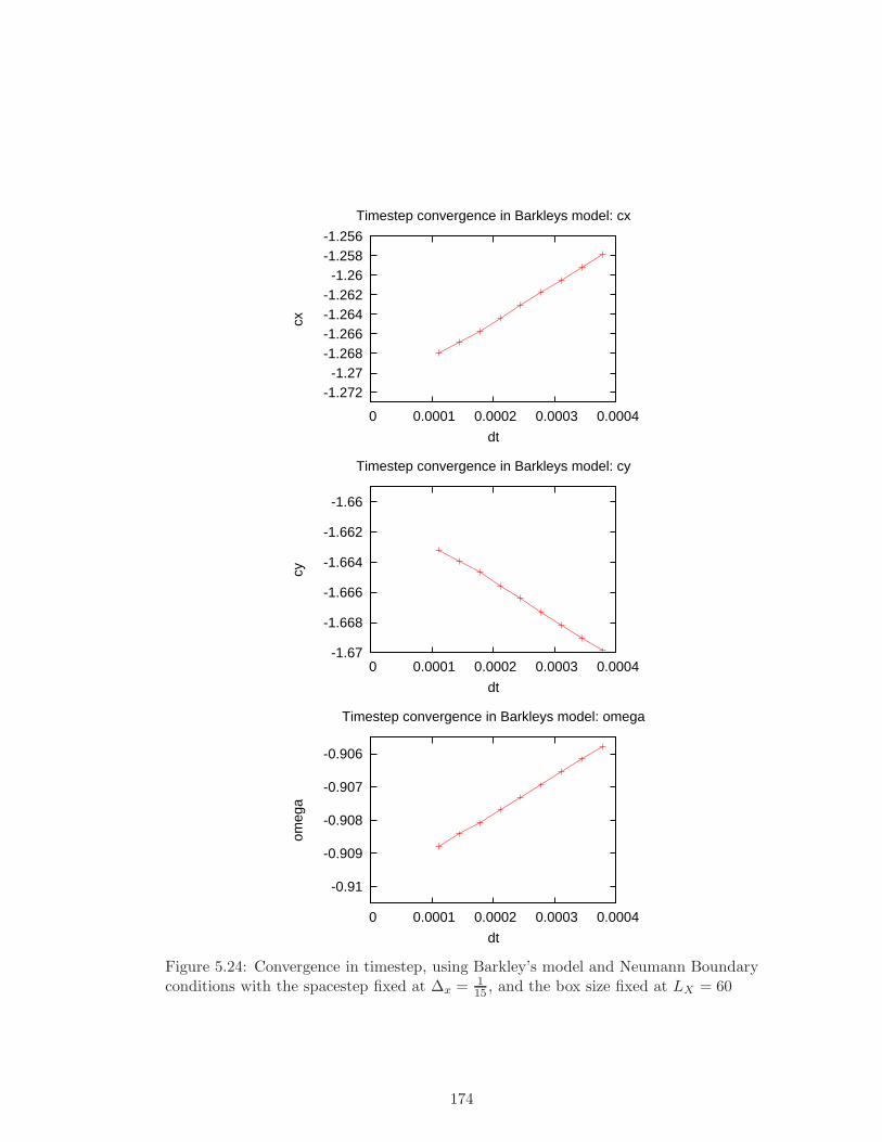
-1.272-1.27
-1.268-1.266-1.264-1.262-1.26
-1.258-1.256
0 0.0001 0.0002 0.0003 0.0004
cx
dt
Timestep convergence in Barkleys model: cx
-1.67
-1.668
-1.666
-1.664
-1.662
-1.66
0 0.0001 0.0002 0.0003 0.0004
cy
dt
Timestep convergence in Barkleys model: cy
-0.91
-0.909
-0.908
-0.907
-0.906
0 0.0001 0.0002 0.0003 0.0004
omeg
a
dt
Timestep convergence in Barkleys model: omega
Figure 5.24: Convergence in timestep, using Barkley’s model and Neumann Boundaryconditions with the spacestep fixed at ∆x = 1
15 , and the box size fixed at LX = 60
174
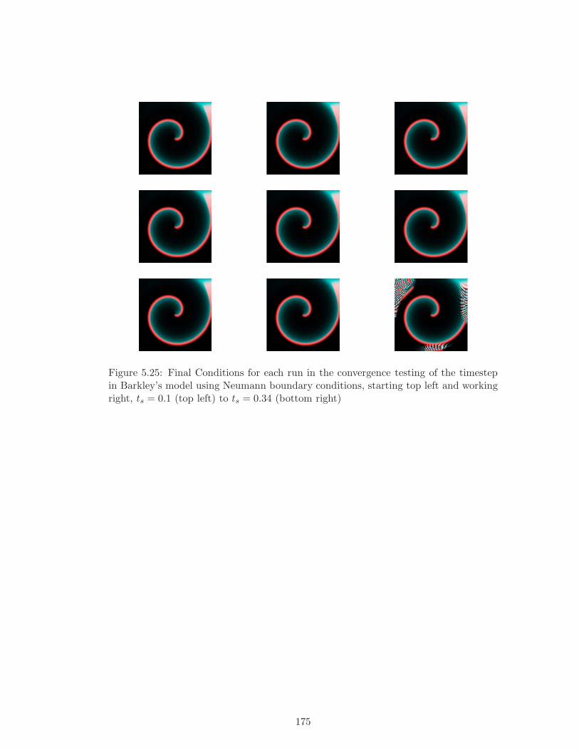
Figure 5.25: Final Conditions for each run in the convergence testing of the timestepin Barkley’s model using Neumann boundary conditions, starting top left and workingright, ts = 0.1 (top left) to ts = 0.34 (bottom right)
175
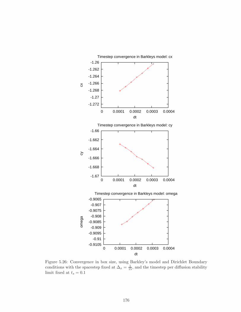
-1.272
-1.27
-1.268
-1.266
-1.264
-1.262
-1.26
0 0.0001 0.0002 0.0003 0.0004
cx
dt
Timestep convergence in Barkleys model: cx
-1.67
-1.668
-1.666
-1.664
-1.662
-1.66
0 0.0001 0.0002 0.0003 0.0004
cy
dt
Timestep convergence in Barkleys model: cy
-0.9105
-0.91
-0.9095
-0.909
-0.9085
-0.908
-0.9075
-0.907
-0.9065
0 0.0001 0.0002 0.0003 0.0004
omeg
a
dt
Timestep convergence in Barkleys model: omega
Figure 5.26: Convergence in box size, using Barkley’s model and Dirichlet Boundaryconditions with the spacestep fixed at ∆x = 1
15 , and the timestep per diffusion stabilitylimit fixed at ts = 0.1
176
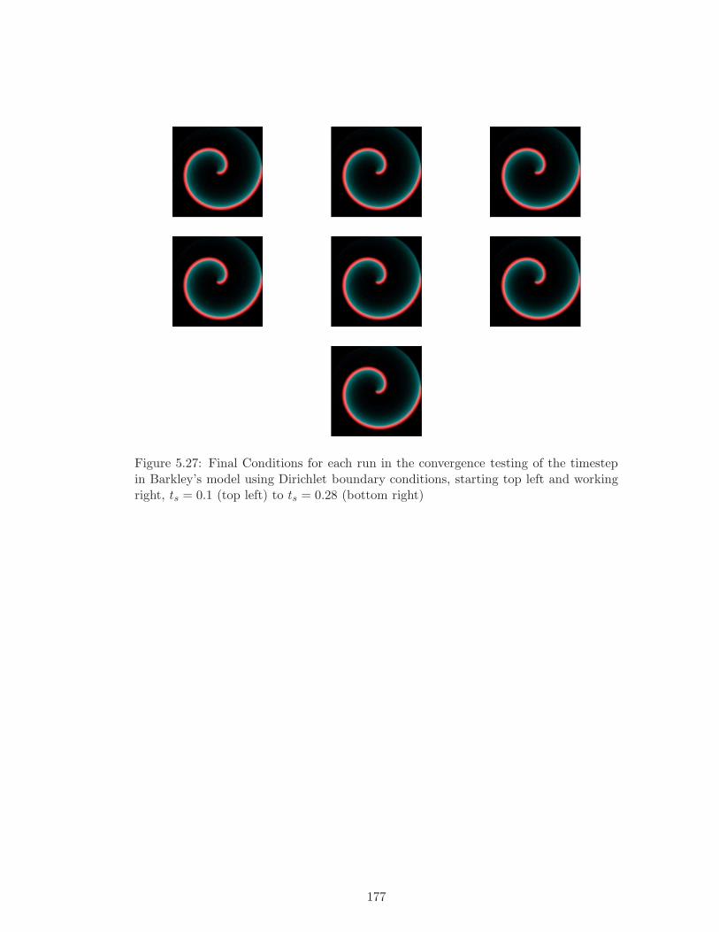
Figure 5.27: Final Conditions for each run in the convergence testing of the timestepin Barkley’s model using Dirichlet boundary conditions, starting top left and workingright, ts = 0.1 (top left) to ts = 0.28 (bottom right)
177
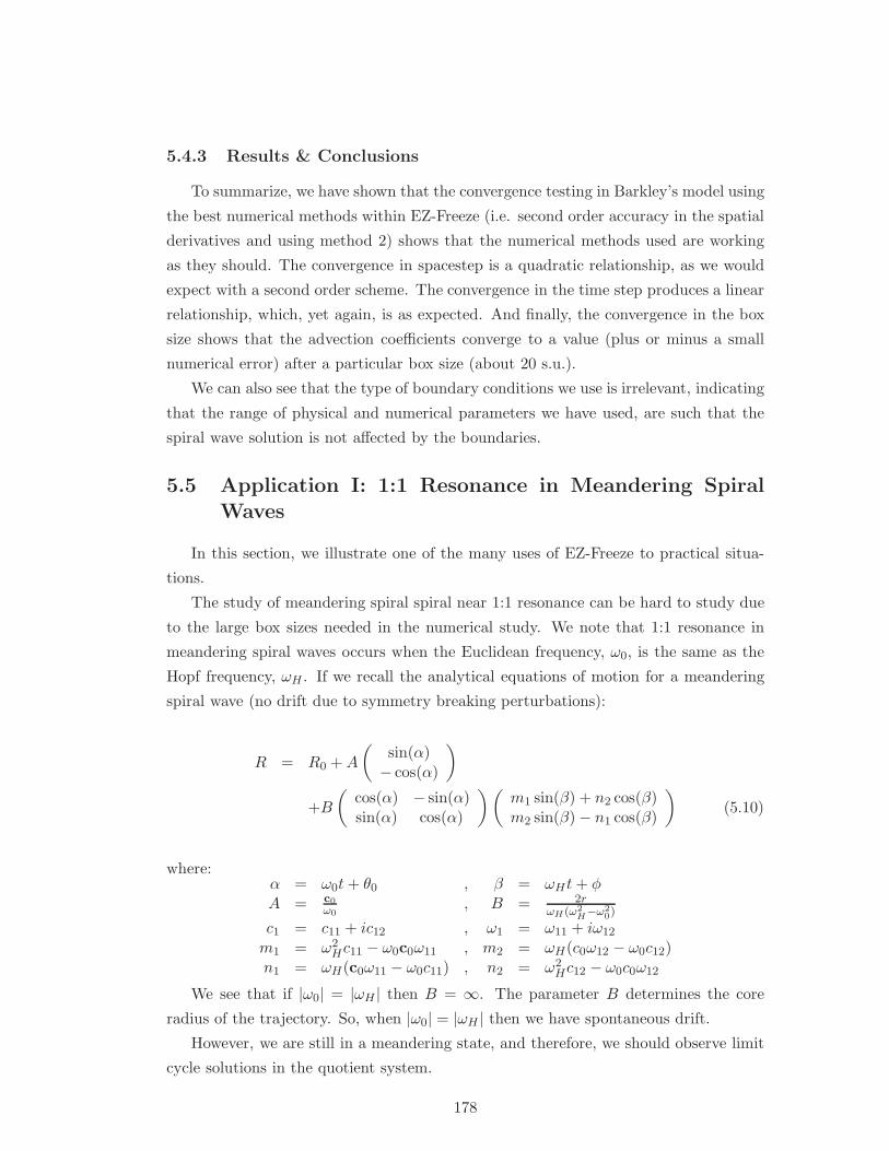
5.4.3 Results & Conclusions
To summarize, we have shown that the convergence testing in Barkley’s model using
the best numerical methods within EZ-Freeze (i.e. second order accuracy in the spatial
derivatives and using method 2) shows that the numerical methods used are working
as they should. The convergence in spacestep is a quadratic relationship, as we would
expect with a second order scheme. The convergence in the time step produces a linear
relationship, which, yet again, is as expected. And finally, the convergence in the box
size shows that the advection coefficients converge to a value (plus or minus a small
numerical error) after a particular box size (about 20 s.u.).
We can also see that the type of boundary conditions we use is irrelevant, indicating
that the range of physical and numerical parameters we have used, are such that the
spiral wave solution is not affected by the boundaries.
5.5 Application I: 1:1 Resonance in Meandering SpiralWaves
In this section, we illustrate one of the many uses of EZ-Freeze to practical situa-
tions.
The study of meandering spiral spiral near 1:1 resonance can be hard to study due
to the large box sizes needed in the numerical study. We note that 1:1 resonance in
meandering spiral waves occurs when the Euclidean frequency, ω0, is the same as the
Hopf frequency, ωH . If we recall the analytical equations of motion for a meandering
spiral wave (no drift due to symmetry breaking perturbations):
R = R0 + A
(
sin(α)− cos(α)
)
+B
(
cos(α) − sin(α)sin(α) cos(α)
)(
m1 sin(β) + n2 cos(β)m2 sin(β)− n1 cos(β)
)
(5.10)
where:α = ω0t + θ0 , β = ωHt + φA = c0
ω0, B = 2r
ωH(ω2H−ω2
0)
c1 = c11 + ic12 , ω1 = ω11 + iω12
m1 = ω2Hc11 − ω0c0ω11 , m2 = ωH(c0ω12 − ω0c12)
n1 = ωH(c0ω11 − ω0c11) , n2 = ω2Hc12 − ω0c0ω12
We see that if |ω0| = |ωH | then B = ∞. The parameter B determines the core
radius of the trajectory. So, when |ω0| = |ωH | then we have spontaneous drift.
However, we are still in a meandering state, and therefore, we should observe limit
cycle solutions in the quotient system.
178
The purpose of this investigation, is to uncover the properties of the quotient system
at 1:1 resonance and determine whether or not these properties are significantly different
than other limit cycles in the vicinity of the 1:1 resonance but not at it.
5.5.1 Method
Throughout this investigation, we shall use the FHN model. The physical and
numerical parameters used in the testing were:
• Box size, LX = 20 s.u.
• Spacestep, ∆x = 0.125 s.u
• Timestep, ∆t = 3.90625 × 10⁻⁴ t.u.
We note that the first tests that we did, which we report here, were done using
the second order accurate numerical scheme, together with method 1. We shall report
on our finding of these results, together with a run of tests done with a second order
scheme and also method 2. The main differences between the results generated using
methods 1 and 2 were the instabilities in the quotient system. However, we found that
there were no obvious anomalies as such when using method 1 and, when compared
with the results from method 2, the results were very similar.
So, the first task we had to do was to locate a point of resonance, or get as close as
we could to a point of resonance. We do this using the “Flower Garden” published by
Winfree in his 1991 paper to get a rough estimate of what parameters we should use
to find 1:1 resonance [63]. This is shown in Fig.(5.28)
What we did was to keep two of the parameters fixed (in this case we fixed γ
and ǫ) and estimate the other parameter (β, which we denote as the free parameter)
from the flower garden. Once we have a rough estimate, we rerun EZ-Freeze using
these parameters and see what trajectory we get. If we find that we have an outward
meandering trajectory (i.e. the petals of the trajectory are facing outwards), then we
need to increase the free parameter. If we get an inward meandering trajectory, we
need to decrease the value of the free parameter. We do this until we get a value of the
parameter which gives us 1:1 resonance or as close to it as we can get.
Once we have found this point, we run EZ-Freeze using the parameters we have
just found. We also run it for some parameter values either side of the value of the free
parameter.
5.5.2 Results
As mentioned in the above section, we used two methods in this investigation.
Therefore, we split this subsection into two; one section for the original results we
179
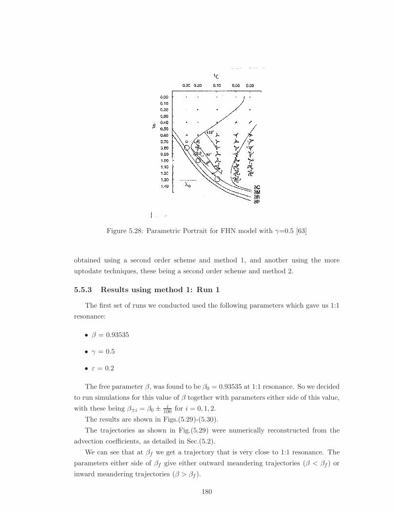
Figure 5.28: Parametric Portrait for FHN model with γ=0.5 [63]
obtained using a second order scheme and method 1, and another using the more
uptodate techniques, these being a second order scheme and method 2.
5.5.3 Results using method 1: Run 1
The first set of runs we conducted used the following parameters which gave us 1:1
resonance:
• β = 0.93535
• γ = 0.5
• ε = 0.2
The free parameter β, was found to be β0 = 0.93535 at 1:1 resonance. So we decided
to run simulations for this value of β together with parameters either side of this value,
with these being β±i = β0 ± i100 for i = 0, 1, 2.
The results are shown in Figs.(5.29)-(5.30).
The trajectories as shown in Fig.(5.29) were numerically reconstructed from the
advection coefficients, as detailed in Sec.(5.2).
We can see that at βf we get a trajectory that is very close to 1:1 resonance. The
parameters either side of βf give either outward meandering trajectories (β < βf ) or
inward meandering trajectories (β > βf ).
180
Also, we note that the length of the trajectory at βf is approximately 360 s.u. If
we were to conduct this in the laboratory frame of reference, we would have needed
a box length of at least 370 s.u. (the extra to allow for the solution to be near, but
not at, the boundary) and a grid size of 2960×2960 to give us a spacestep of 0.125.
Computationally, this would have taken a very long time, but we have conducted this
simulation in approximately two and a half hours. We estimate that this would have
taken about five weeks to perform in a laboratory frame of reference.
If we wanted to, we could let this simulation run for a very long, due to the fact
that the spiral wave never reaches the boundaries. We also conducted the simulations
knowing that the boundaries would not have a great effect on the solution.
Let us look at the quotient system as shown in Fig.(5.30). The plots in the figure
have been drawn to give the reader a good perspective of how the advection coefficients
are related to each other. In each case, we have also included a β-axis to help the reader
compare the plots for each value of β used.
One point that we can note is that there is no obvious difference between the
quotient system corresponding to the 1:1 resonance (shown in blue). We can see that
as we get nearer to the ∂M boundary (this is the boundary separating the regions of
meandering spirals and rigidly rotating spirals (see Fig.(5.28))), the amplitudes of the
limit cycles decrease. This is as expected, since at the ∂M boundary (also note that
this is a Hopf locus), we have that the limit cycles are zero and grow with a 12 power
law [11].
We also note that the limit cycles are quite thin, with one end of the limit cycle
being thicker than the other. If we were to continue the parameters so that we were
getting closer to the Hopf locus, then we should observe a more ellipsoidal limit cycle.
5.5.4 Results using method 1: Run 2
The next set of runs we conducted, were done using βf = 0.812, γ = 0.5 and
ε = 0.25. The other values of β are determined as β±i = β0 ± i200 for i = 0, 1, 2.
The results are shown in Figs.(5.31)-(5.32). As we can see, the results are qualita-
tively very similar. We have quite narrow limit cycles. We also note that we are quite
close to the codim-2 point (the point at which the locus of 1:1 resonance meets the
Hopf locus), we get more ellipsoidal limit cycles.
Again, we see that there is no distinct difference between the limit cycles at the 1:1
resonance points and its environs.
181
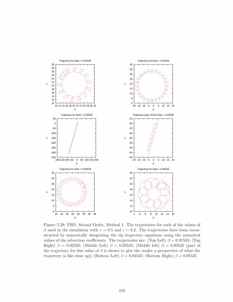
10 12 14 16 18 20 22 24 26 28 30 32
10 12 14 16 18 20 22 24 26 28 30 32
Y
X
Trajectory for beta = 0.91535
0
5
10
15
20
25
30
35
40
-20 -15 -10 -5 0 5 10 15 20
Y
X
Trajectory for beta = 0.92535
-350
-300
-250
-200
-150
-100
-50
0
50
-200-150-100 -50 0 50 100 150 200
Y
X
Trajectory for beta = 0.93535
-55
-50
-45
-40
-35
-30
-25
-20
-15
-20 -15 -10 -5 0 5 10 15 20
Y
X
Trajectory (part of) for beta = 0.93535
0
5
10
15
20
25
30
35
10 15 20 25 30 35 40 45
Y
X
Trajectory for beta = 0.94535
10
12
14
16
18
20
22
24
2 4 6 8 10 12 14 16
Y
X
Trajectory for beta = 0.95535
Figure 5.29: FHN, Second Order, Method 1. The trajectories for each of the values ofβ used in the simulation with γ = 0.5 and ε = 0.2. The trajectories have been recon-structed by numerically integrating the tip trajectory equations using the numericalvalues of the advection coefficients. The trajectories are: (Top Left) β = 0.91535; (TopRight) β = 0.92535; (Middle Left) β = 0.93535; (Middle left) β = 0.93535 (part ofthe trajectory for this value of β is shown to give the reader a perspective of what thetrajectory is like close up); (Bottom Left) β = 0.94535; (Bottom Right) β = 0.95535
182
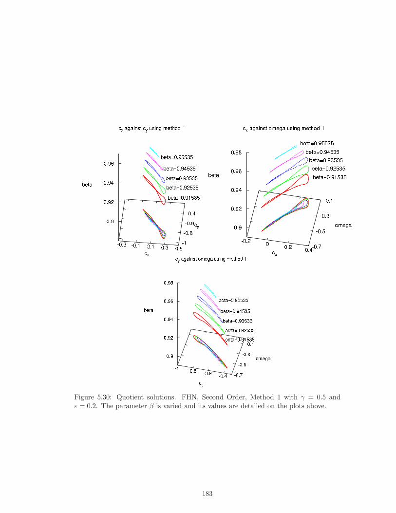
Figure 5.30: Quotient solutions. FHN, Second Order, Method 1 with γ = 0.5 andε = 0.2. The parameter β is varied and its values are detailed on the plots above.
183
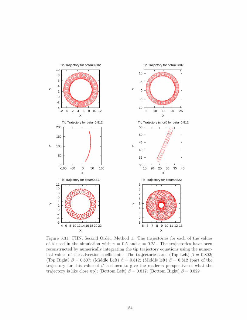
-4
-2
0
2
4
6
8
10
-2 0 2 4 6 8 10 12
Y
X
Tip Trajectory for beta=0.802
-10
-5
0
5
10
5 10 15 20 25
Y
X
Tip Trajectory for beta=0.807
0
50
100
150
200
-100 -50 0 50 100
Y
X
Tip Trajectory for beta=0.812
30
35
40
45
50
55
15 20 25 30 35 40
Y
X
Tip Trajectory (short) for beta=0.812
-6-4-2 0 2 4 6 8
10 12
4 6 8 10 12 14 16 18 20 22
Y
X
Tip Trajectory for beta=0.817
1
2
3
4
5
6
7
8
9
5 6 7 8 9 10 11 12 13
Y
X
Tip Trajectory for beta=0.822
Figure 5.31: FHN, Second Order, Method 1. The trajectories for each of the valuesof β used in the simulation with γ = 0.5 and ε = 0.25. The trajectories have beenreconstructed by numerically integrating the tip trajectory equations using the numer-ical values of the advection coefficients. The trajectories are: (Top Left) β = 0.802;(Top Right) β = 0.807; (Middle Left) β = 0.812; (Middle left) β = 0.812 (part of thetrajectory for this value of β is shown to give the reader a perspective of what thetrajectory is like close up); (Bottom Left) β = 0.817; (Bottom Right) β = 0.822
184
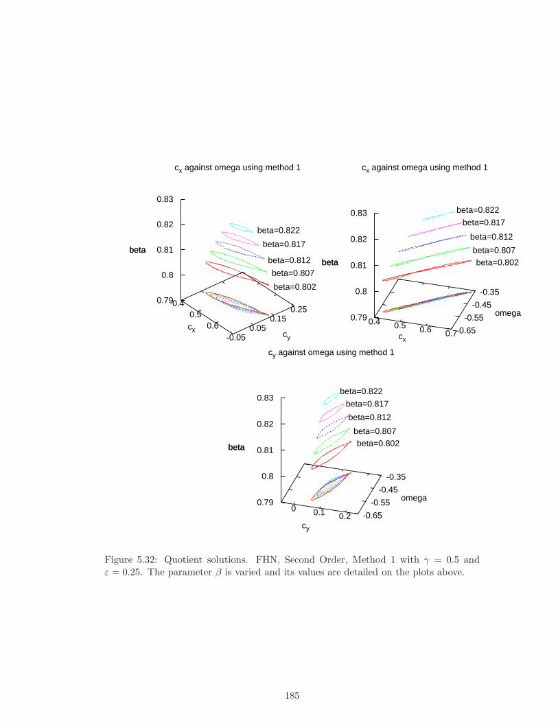
0.4 0.5
0.6-0.05
0.05 0.15
0.25 0.79
0.8
0.81
0.82
0.83
beta
cx against omega using method 1
beta=0.802
beta=0.807
beta=0.812
beta=0.817
beta=0.822
cx cy
beta
0.4 0.5 0.6 0.7-0.65
-0.55
-0.45
-0.35
0.79
0.8
0.81
0.82
0.83
beta
cx against omega using method 1
beta=0.802beta=0.807
beta=0.812
beta=0.817
beta=0.822
cx
omega
beta
0 0.1 0.2 -0.65
-0.55
-0.45
-0.35
0.79
0.8
0.81
0.82
0.83
beta
cy against omega using method 1
beta=0.802beta=0.807
beta=0.812
beta=0.817
beta=0.822
cy
omega
beta
Figure 5.32: Quotient solutions. FHN, Second Order, Method 1 with γ = 0.5 andε = 0.25. The parameter β is varied and its values are detailed on the plots above.
185
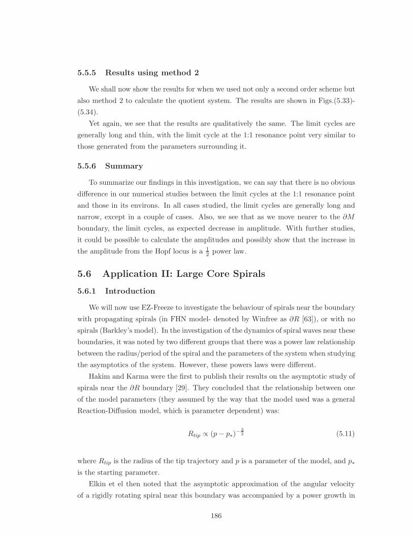
5.5.5 Results using method 2
We shall now show the results for when we used not only a second order scheme but
also method 2 to calculate the quotient system. The results are shown in Figs.(5.33)-
(5.34).
Yet again, we see that the results are qualitatively the same. The limit cycles are
generally long and thin, with the limit cycle at the 1:1 resonance point very similar to
those generated from the parameters surrounding it.
5.5.6 Summary
To summarize our findings in this investigation, we can say that there is no obvious
difference in our numerical studies between the limit cycles at the 1:1 resonance point
and those in its environs. In all cases studied, the limit cycles are generally long and
narrow, except in a couple of cases. Also, we see that as we move nearer to the ∂M
boundary, the limit cycles, as expected decrease in amplitude. With further studies,
it could be possible to calculate the amplitudes and possibly show that the increase in
the amplitude from the Hopf locus is a 12 power law.
5.6 Application II: Large Core Spirals
5.6.1 Introduction
We will now use EZ-Freeze to investigate the behaviour of spirals near the boundary
with propagating spirals (in FHN model- denoted by Winfree as ∂R [63]), or with no
spirals (Barkley’s model). In the investigation of the dynamics of spiral waves near these
boundaries, it was noted by two different groups that there was a power law relationship
between the radius/period of the spiral and the parameters of the system when studying
the asymptotics of the system. However, these powers laws were different.
Hakim and Karma were the first to publish their results on the asymptotic study of
spirals near the ∂R boundary [29]. They concluded that the relationship between one
of the model parameters (they assumed by the way that the model used was a general
Reaction-Diffusion model, which is parameter dependent) was:
Rtip ∝ (p− p∗)− 3
2 (5.11)
where Rtip is the radius of the tip trajectory and p is a parameter of the model, and p∗
is the starting parameter.
Elkin et el then noted that the asymptotic approximation of the angular velocity
of a rigidly rotating spiral near this boundary was accompanied by a power growth in
186
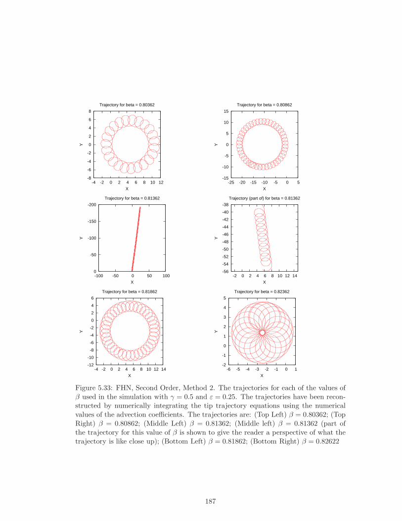
-8
-6
-4
-2
0
2
4
6
8
-4 -2 0 2 4 6 8 10 12
Y
X
Trajectory for beta = 0.80362
-15
-10
-5
0
5
10
15
-25 -20 -15 -10 -5 0 5
Y
X
Trajectory for beta = 0.80862
-200
-150
-100
-50
0-100 -50 0 50 100
Y
X
Trajectory for beta = 0.81362
-56
-54
-52
-50
-48
-46
-44
-42
-40
-38
-2 0 2 4 6 8 10 12 14
Y
X
Trajectory (part of) for beta = 0.81362
-12
-10
-8
-6
-4
-2
0
2
4
6
-4 -2 0 2 4 6 8 10 12 14
Y
X
Trajectory for beta = 0.81862
-2
-1
0
1
2
3
4
5
-6 -5 -4 -3 -2 -1 0 1
Y
X
Trajectory for beta = 0.82362
Figure 5.33: FHN, Second Order, Method 2. The trajectories for each of the values ofβ used in the simulation with γ = 0.5 and ε = 0.25. The trajectories have been recon-structed by numerically integrating the tip trajectory equations using the numericalvalues of the advection coefficients. The trajectories are: (Top Left) β = 0.80362; (TopRight) β = 0.80862; (Middle Left) β = 0.81362; (Middle left) β = 0.81362 (part ofthe trajectory for this value of β is shown to give the reader a perspective of what thetrajectory is like close up); (Bottom Left) β = 0.81862; (Bottom Right) β = 0.82622
187

Figure 5.34: Quotient solutions. FHN, Second Order, Method 2 with γ = 0.5 andε = 0.25. The parameter β is varied and its values are detailed on the plots above:Quotient solutions: (top left) cx vs cy; (top right) cx vs ω; (bottom) cy vs ω
188
the period and radius as [15]:
Rtip ∝ (p− p∗)−1 (5.12)
Hakim and Karma then came back with further analytical evidence of a −32 power
law and extended their studies to further applications such as multiarmed spirals [30].
Therefore, we used EZ-Freeze as a tool to investigate these contradictions and show
our results below.
As Elkin et al noted, the numerical investigation into these claims can prove to be
numerically expensive, in terms of time and system restrictions (memory etc), purely
due to the size of the numerical grid we need. For large core spirals, the core radius of
the spiral wave can be very large and in the numerical simulations which we performed
to generate the following results, we found that the largest radius was approximately
260 space units. For a spacestep of say 0.2, we would need a grid size of at the very
least 1300 × 1300 = 1.69 × 10⁶, for instance. For a standard desktop computer, the
numerical simulations on a grid this size would prove very impractical, if not impossible,
to perform.
So, by using EZ-Freeze (i.e. in a frame of reference comoving with the tip of the
spiral wave), we can afford a smaller box size, thereby eliminating costly computations,
but still get the results as required.
5.6.2 Methods
The advantage of using EZ-Freeze is that is can very quickly determine the values
of the advection coefficients, i.e. the values of cx, cy and ω. From these values we can
calculate the radius of the trajectory by using the formula:
Rtip =|c||ω| =
√
c2x + c2
y
|ω| (5.13)
So, once we have the values of the quotient solution for a given set of parameters,
we can calculate the relationship between the parameters and the ω and Rtip. Consider
the following relationship between between a parameter, a and the period, T , of the
spiral using Hakim & Karma’s results:
T ∝ (p− p∗)− 3
2
⇒ 1
T∝ (p− p∗)
32
⇒ ω ∝ (p− p∗)32 (5.14)
Using the results of Elkin et al, we have, by a similar argument that:
189
T ∝ (p− p∗)−1
ω ∝ p− p∗ (5.15)
Therefore, we investigated which of Eqns.(5.14) and (5.15) are indeed correct, if
either, from a numerical point of view.
We used Barkley’s model with the initial model parameters that were needed to get
us as close to the boundary as we could, being found using Barkley’s so called “Flower
Garden” [9]. These were found to be:
• a = 0.48
• b = 0.05
• ε = 0.02
We also used the following numerical parameters:
• LX = LY = 30 s.u.
• ∆x = 0.125
• ∆t = 3.9 × 10⁻⁴
• (xinc, yinc) = (0,14) (in spaceunits)
We then ran EZ-Freeze several times, each time the value of a was decreased by
0.001. This was repeated until no spiral wave solution was observed.
It was then possible to observe the relationship between the angular frequency ω
and the parameter a.
5.6.3 Observations
Before we show the results of the investigation into which asymptotic method is
numerical verified, we show in Fig.(5.35) the full range of how omega is varying with
the parameter as get very close to the boundary ∂R.
We can see straightaway that there are two distinct regions of this plot. With the
parameters in the range 0.456 ≤ a ≤ 0.48, we have what appears at first sight to be a
linear growth. We then reach a point, which we shall denote as the Critical Point, at
which the growth changes, and then for parameters in the range 0.43 ≤ a < 0.456 we
have a much slower growth (in fact this is decay) and what appears to be a stabilizing
in ω.
We also show in Fig.(5.36) the plot in Fig.(5.35) split over the two noted halves.
190
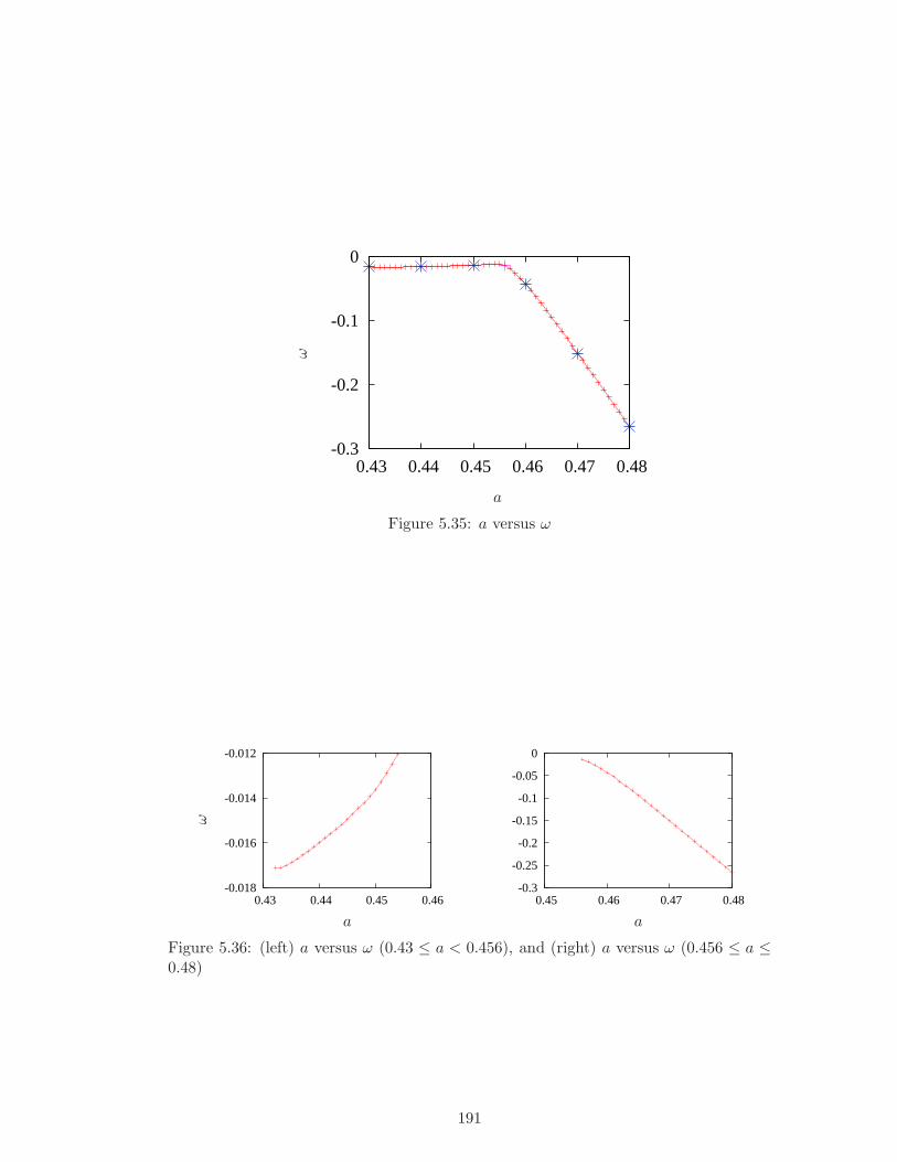
-0.3
-0.2
-0.1
0
0.43 0.44 0.45 0.46 0.47 0.48
a
ω
Figure 5.35: a versus ω
-0.018
-0.016
-0.014
-0.012
0.43 0.44 0.45 0.46
a
ω
-0.3
-0.25
-0.2
-0.15
-0.1
-0.05
0
0.45 0.46 0.47 0.48
a
Figure 5.36: (left) a versus ω (0.43 ≤ a < 0.456), and (right) a versus ω (0.456 ≤ a ≤0.48)
191
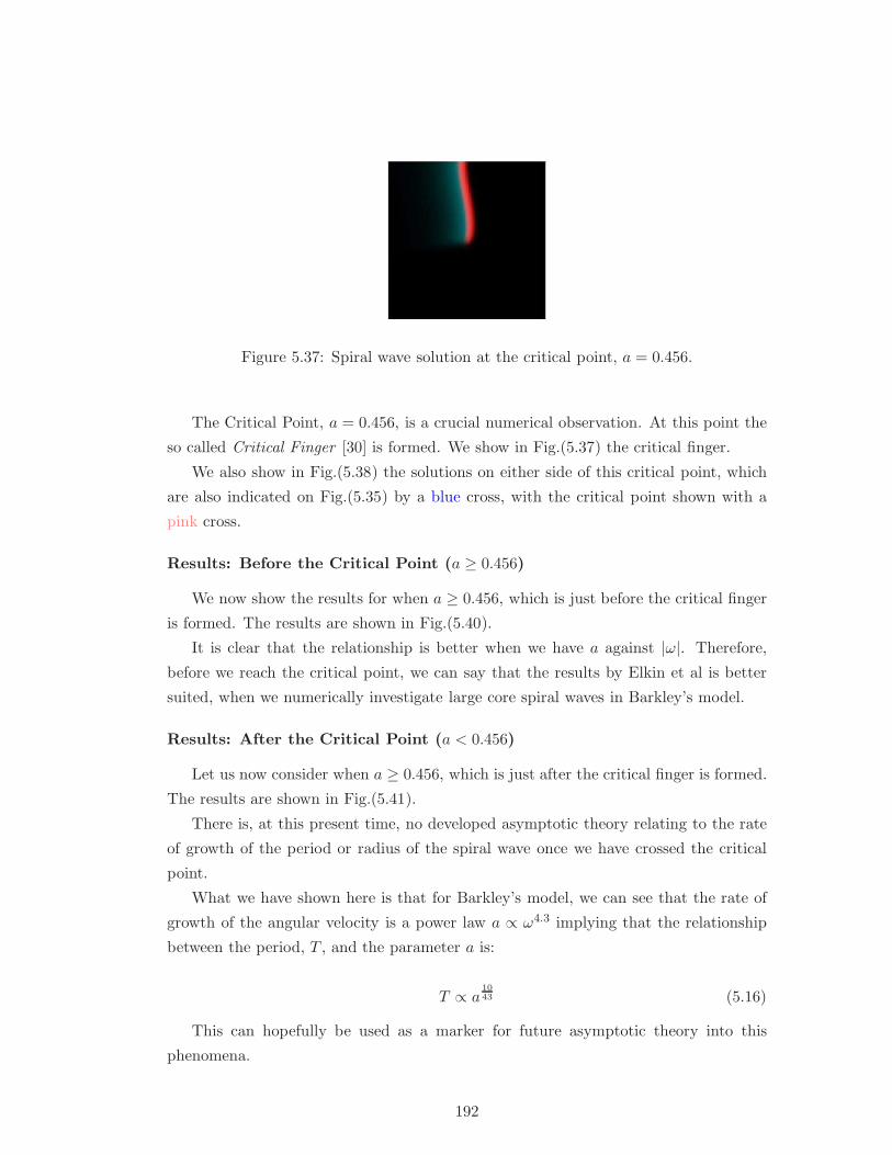
Figure 5.37: Spiral wave solution at the critical point, a = 0.456.
The Critical Point, a = 0.456, is a crucial numerical observation. At this point the
so called Critical Finger [30] is formed. We show in Fig.(5.37) the critical finger.
We also show in Fig.(5.38) the solutions on either side of this critical point, which
are also indicated on Fig.(5.35) by a blue cross, with the critical point shown with a
pink cross.
Results: Before the Critical Point (a ≥ 0.456)
We now show the results for when a ≥ 0.456, which is just before the critical finger
is formed. The results are shown in Fig.(5.40).
It is clear that the relationship is better when we have a against |ω|. Therefore,
before we reach the critical point, we can say that the results by Elkin et al is better
suited, when we numerically investigate large core spiral waves in Barkley’s model.
Results: After the Critical Point (a < 0.456)
Let us now consider when a ≥ 0.456, which is just after the critical finger is formed.
The results are shown in Fig.(5.41).
There is, at this present time, no developed asymptotic theory relating to the rate
of growth of the period or radius of the spiral wave once we have crossed the critical
point.
What we have shown here is that for Barkley’s model, we can see that the rate of
growth of the angular velocity is a power law a ∝ ω4.3 implying that the relationship
between the period, T , and the parameter a is:
T ∝ a1043 (5.16)
This can hopefully be used as a marker for future asymptotic theory into this
phenomena.
192
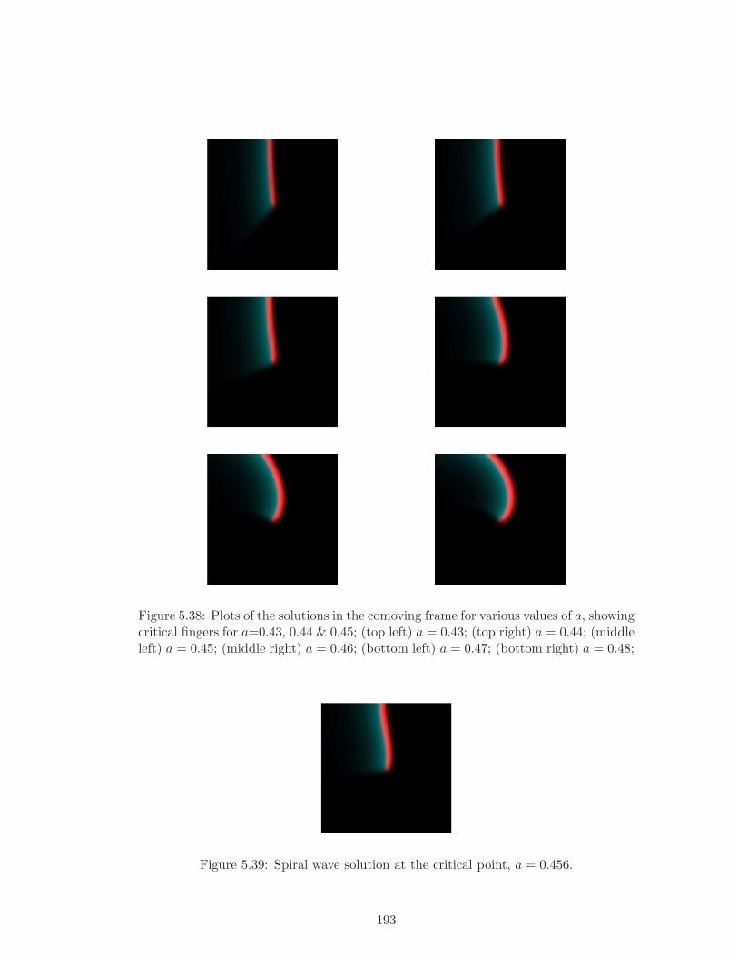
Figure 5.38: Plots of the solutions in the comoving frame for various values of a, showingcritical fingers for a=0.43, 0.44 & 0.45; (top left) a = 0.43; (top right) a = 0.44; (middleleft) a = 0.45; (middle right) a = 0.46; (bottom left) a = 0.47; (bottom right) a = 0.48;
Figure 5.39: Spiral wave solution at the critical point, a = 0.456.
193
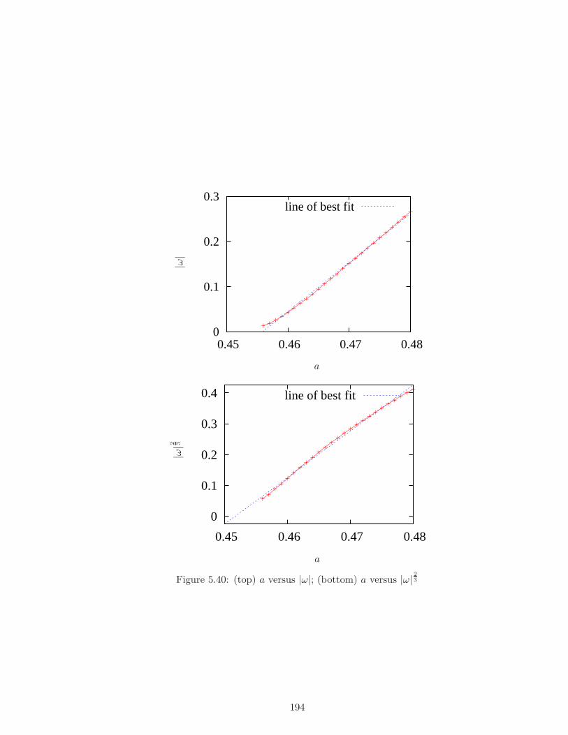
0
0.1
0.2
0.3
0.45 0.46 0.47 0.48
line of best fit
a
|ω|
0
0.1
0.2
0.3
0.4
0.45 0.46 0.47 0.48
line of best fit
a
|ω|2 3
Figure 5.40: (top) a versus |ω|; (bottom) a versus |ω| 23
194
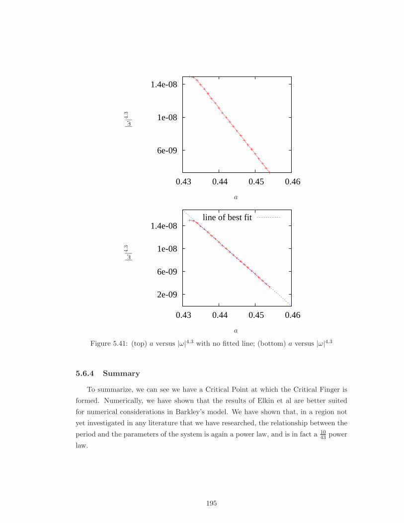
6e-09
1e-08
1.4e-08
0.43 0.44 0.45 0.46
a
|ω|4.
3
2e-09
6e-09
1e-08
1.4e-08
0.43 0.44 0.45 0.46
line of best fit
a
|ω|4.
3
Figure 5.41: (top) a versus |ω|4.3 with no fitted line; (bottom) a versus |ω|4.3
5.6.4 Summary
To summarize, we can see we have a Critical Point at which the Critical Finger is
formed. Numerically, we have shown that the results of Elkin et al are better suited
for numerical considerations in Barkley’s model. We have shown that, in a region not
yet investigated in any literature that we have researched, the relationship between the
period and the parameters of the system is again a power law, and is in fact a 1043 power
law.
195
5.7 Conculsion
To conclude, we have seen that we have shown a numerical method of solving a
system of equations which provides spiral wave solutions in a frame of reference which
is moving with the tip of the spiral wave. This work has resulted in a program called
EZ-Freeze.
We have shown that the numerical methods implemented withing EZ-Freeze provide
accurate solutions, and in some instances, the solutions are produced with remarkable
speed.
We also showed that this method can be used for numerical simulations that have
would have not been possible otherwise, or which would have been numerically expen-
sive in terms of CPU time and memory. The classic case was for the investigation into
large core spirals. There were two conflicting theories which were developed in the
late 1990’s, and it was admitted back then that the numerical investigation into such
methods would have been computationally expensive. We have shown that EZ-Freeze
can be used to investigate such solutions with very little effort. We also confirmed that
from our calculations, the results of Elkin et al proved to be better suited to Barkley’s
model, using the parameters stated. We also showed some initial work into what occurs
after the critical point and what direction any researcher who is thinking of studying
this phenomena should proceed in.
We also showed some results into the study of 1:1 resonance, which we believe
have not yet been shown before. It was interesting to note there that the limit cycles
relating to the 1:1 resonance solutions are not qualitatively different form those of other
meandering solutions. We have also seen that the shapes of the limit cycles are quite
unique and can be studied using EZ-Freeze.
As for future work, we have made the code for EZ-Freeze available online for others
to download and use. There are many uses of EZ-Freeze including the generation of
the value of ω. This is vital information for any researcher of spiral waves, since we can
then determine many things about the spiral wave including the form of the response
function (see Chap.6 for more details).
196
Chapter 6
Numerical Calculation ofResponse Functions
6.1 Introduction
This chapter is concerned with the numerical calculation of the response functions
to the adjoint linearised Reaction-Diffusion system in the rotating frame of reference.
We shall be considering only the FHN system of equations.
We begin the chapter with a review of what a Response Function is and why we
need to study them. We shall also review briefly the literature that has been published
on this subject and how the works presented in the literature can be implemented into
our problem.
We shall then describe the numerical methods used to calculate such functions and
will also introduce a program called evcospi, which numerically calculates the critical
Response Functions. This program is still under development.
We shall then show some examples of how evcospi works, and present some results
from convergence testing that we conducted on the program.
One of the most important factors in generating accurate numerical solutions from
evcospi is the use of accurate initial conditions within the program. We shall present
a review of the way the initial conditions were originally generated, and then present a
more refined and faster approach to generating accurate initial conditions.
This chapter is based on results which are currently in preparation to be published
[19].
197
6.2 Response Functions & Their Importance
6.2.1 The Response Function Problem
We shall be considering rigidly rotating spiral wave solutions in the Reaction-
Diffusion system of equations. We note from Chap.5 that in a frame of reference that
is comoving with the spiral wave with the same angular velocity ω, the rigidly rotating
spiral wave solutions are independent of time. Therefore, the system of equations which
we now consider are:
0 = D∇2v + f(v) + ω∂v
∂θ, (6.1)
v(i)(xc, yc, t) = v∗. (6.2)
where v, f ∈ Rn,D ∈ R
n×n. Also, we have that v = (v(1), v(2), . . . , v(n)), 1 ≤ i ≤ n and
v∗ is a constant (note that the value of v∗ depends on the excitable boundaries of the
medium as determined by the local kinetics). In this case, ω is the angular velocity
of the spiral wave and is actually an unknown constant in this equation. Therefore,
we have n + 1 unknowns, and since Eqn.(6.1) consists of n equations, we require an
additional equation (Eqn.(6.2)) to make it a closed system. This system of equations
gives us spiral wave solutions in a rotating frame of reference.
We recall from Chap.3 that we can formulate an eigenvalue problem, where the
linear operator L in this instance is given by:
Lα = D∇2α+ F(v0)α+ ω∂α
∂θ. (6.3)
where F(v0) = ∂f(v0)∂v
. We note that in this chapter, we are concerned with just the ro-
tating frame of reference, not the comoving as used in Chap.3. The eigenvalue problem
is therefore:
Lφi = λiφi, (6.4)
where the eigenfunctions φi corresponding to the eigenvalues λi are time independent
functions.
Also, we can construct the adjoint eigenvalue problem:
L+ψj = λjψj , (6.5)
198
where the adjoint operator L+ is given by:
L+β = D∇2β + F+(v0)β − ω∂β
∂θ, (6.6)
and F(v0) = ∂f(v0)∂v
.
The eigenfunctions to this adjoint linear operator are what are termed as Response
Functions. So, to calculate them, we need to solve Eqn.(6.5).
Now, as we have seen from Chap.3, when we have a rigidly rotating spiral wave
solution, there are three critical eigenvalues that are located on the imaginary axis.
These eigenvalues are λ0,±1 = 0,±iω, and relate to the symmetry of Reaction-Diffusion-
Advection system.
Therefore, we have that the eigenvalues corresponding to the Response Functions
are λ0,±1 = 0,∓iω.
Also, we have that the Response Functions ψj and the eigenfunctions φi to the
operator L satisfy the biorthogonality condition:
(ψj ,φi) = δji (6.7)
where δji is the Kronecker delta function.
6.2.2 Importance of Response Functions
Before we move on, we shall briefly review the relevant literature regarding the
calculation of response functions and their uses.
It has been said that Response Functions are as important to spiral waves, as mass
is to matter [20]. This is a very strong and critical opinion. But the reasoning behind
such a statement is that you just can’t seem to get away from Response Functions when
studying spiral waves.
Biktasheva et al [20], showed that the velocities of a drifting spiral wave can be
formulated as:
∂tΦ = ǫF0(R,ωt − Φ)
∂tR = ǫF1(R,ωt − Φ)
where the functionals Fn are given by:
199
Fn(t) = einΦ
∫ t+ πω
t− πω
ωdτ
2π
∫ ∫
R2
d2re−inωτ ×
〈ψn (ρ(r −R), θ(r −R) + ωτ − Φ) ,h〉, n = 0,±1
and h is a symmetry breaking perturbation.
Clearly, the Response Functions ψn feature prominently in the prediction of spiral
wave drift.
Similarly, in our research (Chap.3), we see that Response Functions play a vital role
in determining the equations of motion for the tip of a drifting spiral wave:
dR
dt=
[
c0 − ǫ(2(ψ1, h(v0, r, t)) +c0
ω0(ψ0, h(v0, r, t)))
]
eiΘ
dΘ
dt= ω0 − ǫ(ψ0, h(v0, r, t))
where h is a transformed symmetry breaking perturbation.
We have also seen that we can have Floquet Response Functions when we are
considering the dynamics of meandering spiral waves that are drifting. The system of
equations that determine the solution in the space of group orbits, is given by:
dV0
dτ= g(V0)
dV1
dτ= LV1 + S + O(ǫ)
dθ
dτ= ǫ(ψ∗,k)
where
g(V0) = F(V0) + (c0, ∂r)V0 + ω0∂θV0
LV1 =dF(V0)
dV+ (c0, ∂r)V1 + ω0∂θV1
S = (c1, ∂r)V0 + ω1∂θV0 + H(V, t)− (ψ0, H)dV0
dτ
This system is solved using a solvability condition:
(ψn,V0) = 0
(ψn,S) = 0
200
Clearly, we have that the Response Functions, or in this case, the Floquet Response
Functions featuring prominently in the equations.
Therefore, it is evident that the response functions are extremely important in the
study of spiral waves.
6.3 Numerical Implementation
We shall now review the methods that are employed into evcospi which numerically
solve the adjoint eigenvalue problem to give us the Response Function solutions:
L+ψj = λjψj (6.8)
where L+ is given by (6.6). We note that in the definition of L, we have two unknown
variables built into the operator - v0 and ω.
Therefore, the first problem that we need to solve is to find what v0 and ω are.
Once we have found these, we can substitute them into (6.8) and find the Response
Functions.
So, in the next couple of sections we shall describe the general methods that we will
be using to find the initial solutions and then the eigenvalues and eigenfunctions for a
general eigenvalue problem.
The techniques implemented into evcospi are based on methods documented by
Wheeler and Barkley [58].
6.3.1 Calculation of the initial conditions
Firstly, we note that we are now going to consider just a general eigenvalue problem
of the form:
Lφi = λiφi
where L is given by (6.3). As mentioned, we need to find an initial steady state
solution v0 and also the rotational velocity ω. The first step we take is to get an initial
approximation to v0 and ω. This means solving the following equations:
0 = D∇2v0 + f(v0) + ω∂v0
∂θ(6.9)
v(i)0 (xc, yc, t) = v∗
201
where v0, f ∈ Rn, D ∈ R
n×n, v0 = (v(1)0 , v
(2)0 , . . . , v
(n)0 ), 1 ≤ i ≤ n, and v∗ is a carefully
chosen value depending on the local kinetics of the model being used and which is
chosen within the region of excitability of the model.
There are several ways to generate an initial approximation to v0, and these methods
are described in Sec.(6.4).
So, once we get an initial approximation to v0 and ω, we then need to find just
how good this initial approximation is. We do this by calculating the norm of the RHS
of Eqn.(6.9), and we call upon the subroutine set out in LAPACK (this is a standard
numerical analysis package used to solve a large number of linear equations)[3]. The
routine called upon is dnrm2_, which calculates the residual norm.
We then apply Newton Iterations to the nonlinear problem (6.9) and repeat these
iterations until the solution converges to a specified order. After each iteration, we
perform a check of how good the solution is after that iteration by calling the routine
dnrm2_.
6.3.2 Numerical Calculation of the eigenvalues and eigenfunctions
Once we have a refined steady state solution and value of ω we then need to solve
the following problem:
L+ψj = λjψj
For the rest of this section, we shall consider a general eigenvalue problem and
describe (briefly) the methods which we used to solve this, which by the way, are
implemented into evcospi.
Consider a general eigenvalue problem:
Ax = µx (6.10)
where x ∈ Rn is the eigenvector corresponding to the eigenvalue µ, and A ∈ R
n×n.
We would like to solve system (6.10) numerically to find both the eigenvalues and
corresponding eigenvectors, in the knowledge that we know what the eigenvalues are
from theoretical considerations.
Let us assume that we can approximate the eigenvalues µ by ν, i.e. µ ≈ ν, where ν
are eigenvalues of matrix B. We also assume that the eigenvectors corresponding to ν
are the same as those for µ:
202
Bx = νx (6.11)
Using a Cayley transform, we can establish a relationship between the matrices A
and B:
A = (ζI + B)−1(ξI + B)
where ξ, ζ ∈ R. Similarly, we have a relationship between the eigenvalues:
µ =ξ + ν
ζ + ν
By doing this transformation, we can transform the eigenvalues that we want to the
eigenvalues with the greatest magnitude, simply by varying the two parameters ξ and
ζ.
The next step is to use Arnoldi Iterations to find the dominant eigenvalues. This is
a more stable form of the Power Iteration. A Power Iteration to solve the eigenvalue
problem (6.11) is when we take an arbitrary vector, x, which we assume to be normal-
ized (i.e. ||x|| = 1), and apply matrix B to it. Each iteration consists of normalizing
the previously found vector and applying B to it.
For the eigenvalue problem (6.11), let us assume that the eigenvector has the form:
x =∑
i
aixi
Applying Power Iterations we get:
Bx =∑
i
λiaixi
B2x =∑
i
λ2i aixi
. . . . . .
Bnx =∑
i
λni aixi
Now, as n→∞, we find that the largest eigenvalue dominates and that:
Bnx = λn∗a∗x∗(1 + o(1))
203
Hence we can establish the eigenvector x∗ corresponding to the eigenvalue with the
largest absolute value, λ∗. An estimate of this eigenvalue is given by [41]:
λ∗ =xT∗ Bx∗
xT∗ x∗
The Arnoldi Method is very similar to the Power Iteration. However, instead of
iterating just one vector x, it iterates a finite dimensional “Krylov” subspace, the basis
of which is orthonormalized after each iteration by Gram-Schmidt orthogonalization.
The program evcospi takes advantage of the numerical package ARPACK, which
includes all the routines necessary to use the Arnoldi method [46]. Also, to use some of
the techniques used in the Newton Iterations, it utilises the routines found in LAPACK
[3].
6.4 Generation of Initial Conditions
In this section we shall describe the methods that are used to firstly generate the
initial conditions (IC’s) and then how they are implemented into evcospi. We will
then describe a method which we have devised to generate initial conditions quicker
then the other methods but still retaining high orders of accuracy.
The accuracy of initial conditions within evcospi is critical, since the program is
sensitive to initial conditions. If we had a set of initial conditions that are not very
accurate, the performing Newton Iterations may result in the initial solution not being
refined, and therefore the calculation of the Response Functions not being made.
6.4.1 Generation of IC’s using EZ-Spiral
There are three methods by which evcospi IC’s are generated. The first is by using
the program EZ-Spiral; the next is using a program called AUTO; and the last method
is using the final conditions generated from a run of evcospi as the initial conditions
for the next run. We shall describe two of these methods below (EZ-Spiral and EZ-
Freeze). We will not go into any sort of detail regarding AUTO, since this method is
due to be made redundant within evcospi.
As mentioned earlier on in this thesis, EZ-Spiral is a program that is available to
download free of charge and which generates spiral wave solutions using fast numerical
calculations [8, 6]. It originally incorporated Barkley’s model but it has been adjusted
to include FHN kinetics.
The idea is to generate a rigidly rotating spiral wave solution whose center of ro-
tation is as close to the center of the box as possible. When a wave is initiated, the
user can plot the tip path of the spiral wave. It was advised to move the spiral wave
204
using the arrow keys so that the spiral is rotating around a point which is as close to
the center of the box as possible. There are some major disadvantages to this. Firstly,
how do you tell when it is rotating around the center of the box? Do you get a ruler
out and measure, or do you just go “by eye”? This is a very crude method and one
which actually threw up problems when trying to implement it into evcospi.
The next task that needs to be done is to find what the rotational velocity, ω, is.
To do this the user was advised to plot the trajectory of the u-field against time as
recorded in the history.dat file produced by EZ-Spiral. From this plot, the user could
estimate the period, T , of the spiral (by measuring the time period between successive
peaks for instance) and then calculate by hand the angular velocity using:
ω =2π
T
The final conditions generated by EZ-Spiral could then be used for the IC’s in
evcospi.
How the IC’s are read into evcospi is of vital importance. The IC’s must also be as
accurate as possible in order to generate accurate Response Functions. For EZ-Spiral
the major problem was the fact that the final conditions are generated on a cartesian
grid, but evcospi requires the IC’s in polar form. So, we must transform the data from
a cartesian grid to a polar grid.
The program evcospi, does this by taking the angular step as given by the user
in the command line and the EZ-Spiral final conditions file, working out what the
cartesian equivalent is for each polar grid point, and calculating the nearest cartesian
grid point to each polar point. The u and v values for each polar point are taken as
the values of u and v fields at the nearest cartesian grid point to each polar point.
The main and obvious disadvantage to this is that the allocation of the u and v
values to each grid point is very crude. The method just picks out the nearest u and
v values and allocates them to the polar grid coordinates. This therefore, provides
inaccuracies within the solution and therefore the performance of Newton Iterations on
that solution greatly increases the chances of the solution not converging.
6.4.2 Generation of IC’s using EZ-Freeze
We shall now describe the method with which EZ-Freeze can be used to generate
IC’s for evcospi.
We know from Chap.5 that EZ-Freeze has several uses. One of these uses is to
calculate ω, the rotational velocity of a spiral wave. We have also shown that this value
is very good in terms of numerical accuracy.
205
So, there are two processes which we use within EZ-Freeze which we will utilise to
give use accurate IC’s for evcospi.
The first is to calculate ω for a rigidly rotating spiral wave. This is achieved by the
following algorithm:
1. Initiate a spiral wave with the desired physical and numerical parameters. Note
that the numerical parameters must be sufficient to give us an accurate spiral
wave solution (see convergence testing);
2. Once the wave has settled from its transient period to a rigidly rotation spiral
wave (done by observing the tip trajectory), switch on the advection terms by
pressing z;
3. The wave will oscillate for a brief moment and then the advection coefficients (cx,
cy and ω) will converge to their final values;
4. Either terminate the program by pressing q or allow the program to run through it
full number of timesteps as determined in the task.dat file (denoted by nsteps).
A final conditions file fc_ecx.dat will be generated, amongst other files, which
is written in the “own” conditions usable by evcospi. We shall now describe the
algorithm incorporated into EZ-Freeze which generates these conditions.
Algorithm for generating the file fc ecx.dat
EZ-Freeze can be used to calculate not only the angular velocity, ω, but also the
translational velocities, c = (cx, cy), of the spiral. We note from Sec.(2.2.3) that the
radius of the trajectory is given by:
Rc =|c||ω| =
√
c2x + c2
y
|ω| (6.12)
Our next task is to determine the center of rotation of spiral. This is a straightfor-
ward task and, by considering Fig.(6.1), we can see that the center of rotation is given
by:
(xc, yc) = (X,Y )− nRcsgn(ω)
where n is the unit normal along the radius Rc. This can further be reduced by using
Eqn.(6.12):
206
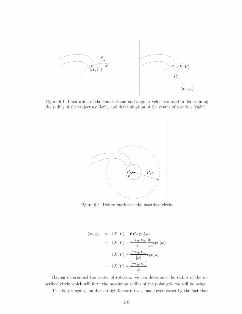
(X,Y )ω
c
(X,Y )
Rc
(xc, yc)
Figure 6.1: Illustration of the translational and angular velocities used in determiningthe radius of the trajectory (left), and determination of the center of rotation (right).
RICRc
Figure 6.2: Determination of the inscribed circle.
(xc, yc) = (X,Y )− nRcsgn(ω)
= (X,Y )− (−cy, cx)
|c||c||ω|sgn(ω)
= (X,Y )− (−cy, cx)
|ω| sgn(ω)
= (X,Y )− (−cy, cx)
ω
Having determined the center of rotation, we can determine the radius of the in-
scribed circle which will form the maximum radius of the polar grid we will be using.
This is, yet again, another straightforward task, made even easier by the fact that
207
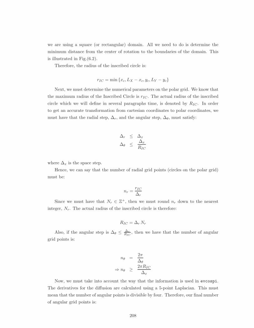
we are using a square (or rectangular) domain. All we need to do is determine the
minimum distance from the center of rotation to the boundaries of the domain. This
is illustrated in Fig.(6.2).
Therefore, the radius of the inscribed circle is:
rIC = min xc, LX − xc, yc, LY − yc
Next, we must determine the numerical parameters on the polar grid. We know that
the maximum radius of the Inscribed Circle is rIC . The actual radius of the inscribed
circle which we will define in several paragraphs time, is denoted by RIC . In order
to get an accurate transformation from cartesian coordinates to polar coordinates, we
must have that the radial step, ∆r, and the angular step, ∆θ, must satisfy:
∆r ≤ ∆x
∆θ ≤ ∆x
RIC
where ∆x is the space step.
Hence, we can say that the number of radial grid points (circles on the polar grid)
must be:
nr =rIC
∆r
Since we must have that Nr ∈ Z+, then we must round nr down to the nearest
integer, Nr. The actual radius of the inscribed circle is therefore:
RIC = ∆r Nr
Also, if the angular step is ∆θ ≤ ∆x
RIC, then we have that the number of angular
grid points is:
nθ =2π
∆θ
⇒ nθ ≥ 2πRIC
∆x
Now, we must take into account the way that the information is used in evcospi.
The derivatives for the diffusion are calculated using a 5-point Laplacian. This must
mean that the number of angular points is divisible by four. Therefore, our final number
of angular grid points is:
208
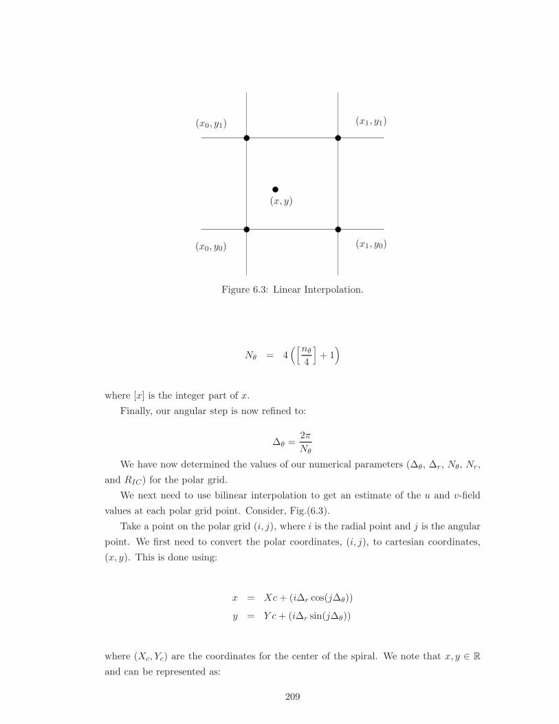
(x0, y1)
(x0, y0)
(x1, y1)
(x1, y0)
(x, y)
Figure 6.3: Linear Interpolation.
Nθ = 4([nθ
4
]
+ 1)
where [x] is the integer part of x.
Finally, our angular step is now refined to:
∆θ =2π
Nθ
We have now determined the values of our numerical parameters (∆θ, ∆r, Nθ, Nr,
and RIC) for the polar grid.
We next need to use bilinear interpolation to get an estimate of the u and v-field
values at each polar grid point. Consider, Fig.(6.3).
Take a point on the polar grid (i, j), where i is the radial point and j is the angular
point. We first need to convert the polar coordinates, (i, j), to cartesian coordinates,
(x, y). This is done using:
x = Xc + (i∆r cos(j∆θ))
y = Y c + (i∆r sin(j∆θ))
where (Xc, Yc) are the coordinates for the center of the spiral. We note that x, y ∈ R
and can be represented as:
209
x = x0 + p
y = y0 + q
where x0, y0 ∈ Z, and 0 < p < 1, 0 < q < 1.
The value of the point u(x, y) using bilinear interpolation is:
u(x, y) = u(x0, y0)(1 − p)(1− q) + u(x1, y0)p(1− q)
+u(x0, y1)(1− p)q + u(x1, y1)pq
where x1 = x0 + 1 and y1 = y0 + 1. This is done for all points on the polar grid.
The next task is to make sure that data calculated above which is written to the
file fc_ecx.dat, is in an order which can be read using evcospi’s “own” format.
Once this is done, the file can be copied to a directory which is accessible by evcospi
and then can be used as the the user sees fit.
6.5 Examples: ec.x
We shall now consider an example using the FHN model and we shall generate the
IC’s for a rigidly rotating spiral wave using EZ-Freeze. We refer the reader to Chap.5
for details of the FHN model and how this model is implemented into the code.
Using, a second order accurate scheme, the parameters chosen in the cartesian grid
were:
• Model Parameters: a=0.68, b=0.5, ε = 0.3
• Numerical Parameters: Lx = Ly=30 s.u., ∆x = 13 , ts=0.05⇒ ∆t = 1.389×10⁻³.
We set the second pinning condition at (xinc, yinc) = (0, 203 ) s.u
We found that the values of the advection coeffecients were cx = 0.5203459859,
cy = −0.2124501765 and ω = −0.5724548697. The radius of the tip trajectory was
therefore Rc = 0.981816 s.u., which means that the center of rotation was at (xc, yc) =
(14.8174, 15.2814) and the radius of the inscribed circle was RIC = 14.7186 s.u.
Therefore, the numerical & physical parameters on the polar grid were found to be:
• ∆r = 13 , Nr=43, ∆θ = 2.27652 × 10⁻², Nθ=276.
We then ran evcospi using the IC’s generated above, and got the results as shown
in Figs.(6.4)-(6.5)
210
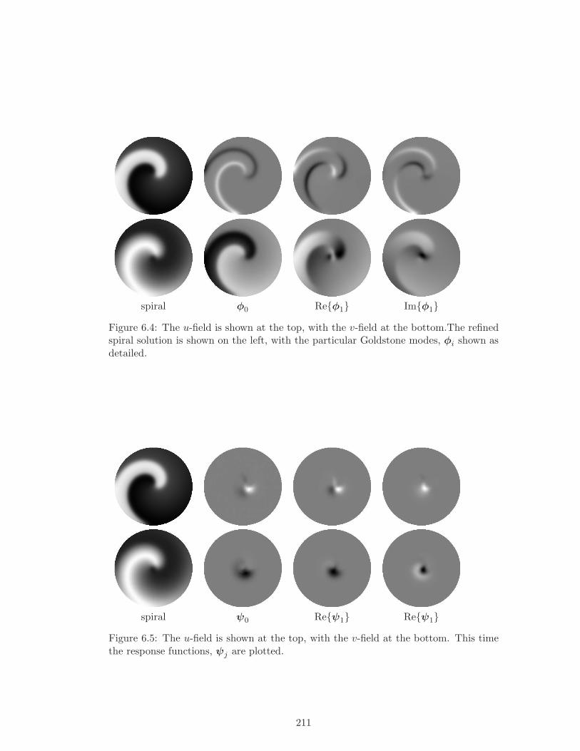
spiral φ0 Reφ1 Imφ1
Figure 6.4: The u-field is shown at the top, with the v-field at the bottom.The refinedspiral solution is shown on the left, with the particular Goldstone modes, φi shown asdetailed.
spiral ψ0 Reψ1 Reψ1
Figure 6.5: The u-field is shown at the top, with the v-field at the bottom. This timethe response functions, ψj are plotted.
211
The main observation is the localisation of the response functions near the core of
the spiral. This localisation was conjectured by Biktashev [ref], shown numerically by
[refs] for the Complex Ginzburg Landau Equation, but first calculated accurately by
Biktasheva et al [19]. This localisation is a surprising feature of response functions and
can be taken advantage numerically by, for example, calculating the drift of the spiral
wave considering only the core of the spiral. Indeed, it can be said that the speed of a
drifting spiral wave is determined only by what is happening at the core of the spiral.
6.6 Convergence Testing
We will detail the work we did in initiating the convergence testing for evcospi.
The purpose of the program is to see how accurate the solutions were by considering
the variation of the numerical parameters.
We conducted tests for convergence in the radial step, angular step, and disk radius,
with the idea being to see how accurately the eigenvalues were calculated. We recall
that from analytical considerations there are three critical eigenvalues - λ0,±1 = 0,±iω.
Numerical calculations always carry an error and therefore, by comparing the numeri-
cally calculated eigenvalues to the values we know they should be, then we can see how
good our numerical approximation is.
6.6.1 Methods
We started with initial conditions generated using EZ-Spiral and continued the
parameter to the following set of “ideal” parameters.
• Numerical Parameters
– disk radius = 40
– Number of angular points = 76
– number of radial points = 250
• Model Parameters
– a = 0.5
– b = 0.68
– ε = 0.3
Once these IC’s are generated, then we decrease one of the parameters from it’s
ideal value using continuation by a suitably chosen step in that parameter. We repeat
this procedure, decreasing the parameter each time by the fixed step, until the solution
no longer exists.
212
We repeat this for all the numerical parameters.
6.6.2 Disk Size
We show the results of the convergence testing of the disk size in Fig.(6.6). We
started with a disk radius size of 40 s.u. and worked our way back to 4 s.u. in steps of
4 s.u.
We can see that the eigenvalues converge to their absolute values between disk sizes
8 and 12 s.u.
Let us represent the eigenvalues as:
λn = Λn + δn
where λn is the actual numerically calculated eigenvalue, Λn = inω, ω is the numerically
found value, and δn is the error. We call Λn the converged eigenvalue. We also note
that n = 0,±1.
For disk sizes greater than 12 s.u. we note that the value of the angular velocity
and the converged eigenvalues are:
• Linear operator L:
– ω = -0.582022542082
– Λ1 = 0.00020000998-i0.584547959642
– Λ0 = 1.0×10⁻¹³-i1.0×10−27
– Λ−1 = 0.00020000998+i0.584547959642
• Adjoint linear operator L+:
– ω = -0.582022542082
– Λ1 = 0.00020001193+i0.584547960827
– Λ0 = 1.0×10⁻⁹-i1.0×10−24
– Λ−1 = 0.00020001193-i0.584547960827
So we can see that the eigenvalue have converged to a very accurately calculated
figures. We see that the real parts must be zero but that they are of the orders
1.0 × 10⁻¹³ and 1.0 × 10⁻⁹ for the zero eigenvalue and adjoint eigenvalue respectively,
and of the order 1.0 × 10⁻⁴ for the other eigenvalues. The imaginary parts are of
the orders 1.0 × 10⁻²⁷ and 1.0 × 10⁻²⁴ for the zero eigenvalue and adjoint eigenvalue
respectively, and 1.0 × 10⁻³ for the others.
So a high order of accuracy is achieved.
213
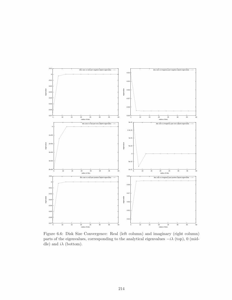
-0.07
-0.06
-0.05
-0.04
-0.03
-0.02
-0.01
0
0.01
5 10 15 20 25 30 35 40
eige
nval
ue
radius of disc
disc size vs real part negative adjoint eigenvalue
-0.59
-0.58
-0.57
-0.56
-0.55
-0.54
5 10 15 20 25 30 35 40
eige
nval
ue
radius of disc
disc size vs imaginery part negative adjoint eigenvalue
-5e-06
-4e-06
-3e-06
-2e-06
-1e-06
0
5 10 15 20 25 30 35 40
eige
nval
ue
radius of disc
disc size vs real part zero adjoint eigenvalue
-1e-21
-5e-22
0
5e-22
1e-21
1.5e-21
2e-21
5 10 15 20 25 30 35 40
eige
nval
ue
radius of disc
disc size vs imaginery part zero adjoint eigenvalue
-0.07
-0.06
-0.05
-0.04
-0.03
-0.02
-0.01
0
0.01
5 10 15 20 25 30 35 40
eige
nval
ue
radius of disc
disc size vs real part positive adjoint eigenvalue
0.54
0.55
0.56
0.57
0.58
0.59
5 10 15 20 25 30 35 40
eige
nval
ue
radius of disc
disc size vs imaginery part positive adjoint eigenvalue
Figure 6.6: Disk Size Convergence: Real (left column) and imaginary (right column)parts of the eigenvalues, corresponding to the analytical eigenvalues −iλ (top), 0 (mid-dle) and iλ (bottom).
214
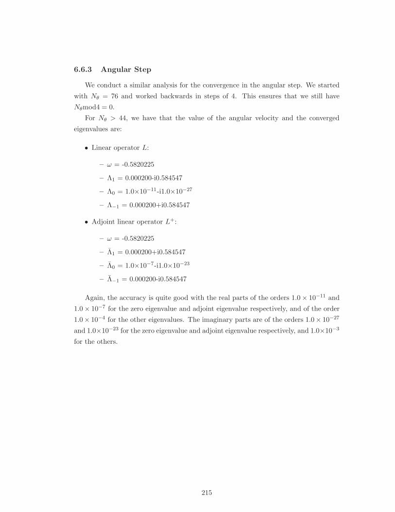
6.6.3 Angular Step
We conduct a similar analysis for the convergence in the angular step. We started
with Nθ = 76 and worked backwards in steps of 4. This ensures that we still have
Nθmod4 = 0.
For Nθ > 44, we have that the value of the angular velocity and the converged
eigenvalues are:
• Linear operator L:
– ω = -0.5820225
– Λ1 = 0.000200-i0.584547
– Λ0 = 1.0×10⁻¹¹-i1.0×10−27
– Λ−1 = 0.000200+i0.584547
• Adjoint linear operator L+:
– ω = -0.5820225
– Λ1 = 0.000200+i0.584547
– Λ0 = 1.0×10⁻⁷-i1.0×10−23
– Λ−1 = 0.000200-i0.584547
Again, the accuracy is quite good with the real parts of the orders 1.0× 10⁻¹¹ and
1.0× 10⁻⁷ for the zero eigenvalue and adjoint eigenvalue respectively, and of the order
1.0× 10⁻⁴ for the other eigenvalues. The imaginary parts are of the orders 1.0× 10⁻²⁷
and 1.0×10⁻²³ for the zero eigenvalue and adjoint eigenvalue respectively, and 1.0×10⁻³
for the others.
215
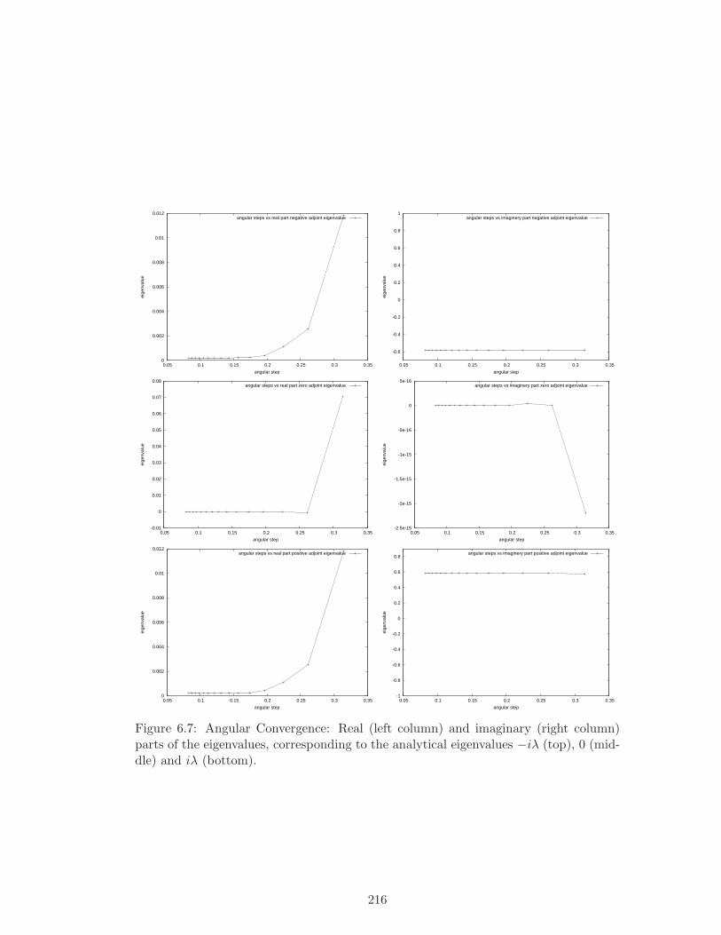
0
0.002
0.004
0.006
0.008
0.01
0.012
0.05 0.1 0.15 0.2 0.25 0.3 0.35
eige
nval
ue
angular step
angular steps vs real part negative adjoint eigenvalue
-0.6
-0.4
-0.2
0
0.2
0.4
0.6
0.8
1
0.05 0.1 0.15 0.2 0.25 0.3 0.35
eige
nval
ue
angular step
angular steps vs imaginery part negative adjoint eigenvalue
-0.01
0
0.01
0.02
0.03
0.04
0.05
0.06
0.07
0.08
0.05 0.1 0.15 0.2 0.25 0.3 0.35
eige
nval
ue
angular step
angular steps vs real part zero adjoint eigenvalue
-2.5e-15
-2e-15
-1.5e-15
-1e-15
-5e-16
0
5e-16
0.05 0.1 0.15 0.2 0.25 0.3 0.35
eige
nval
ue
angular step
angular steps vs imaginery part zero adjoint eigenvalue
0
0.002
0.004
0.006
0.008
0.01
0.012
0.05 0.1 0.15 0.2 0.25 0.3 0.35
eige
nval
ue
angular step
angular steps vs real part positive adjoint eigenvalue
-1
-0.8
-0.6
-0.4
-0.2
0
0.2
0.4
0.6
0.8
0.05 0.1 0.15 0.2 0.25 0.3 0.35
eige
nval
ue
angular step
angular steps vs imaginery part positive adjoint eigenvalue
Figure 6.7: Angular Convergence: Real (left column) and imaginary (right column)parts of the eigenvalues, corresponding to the analytical eigenvalues −iλ (top), 0 (mid-dle) and iλ (bottom).
216
6.6.4 Radial Step
We now consider the plots for convergence in the radial step. We kept the box
size fixed at 10 s.u. and varied the number of radial grid points, therefore giving us
convergence in the Radial step. Since the numerical radial derivatives are to second
order, we plot the results with the square of the radial step.
We find that for the real parts of the eigenvalues, convergence happens for Nr > 100.
We also note there are instabilities in the plot for real part of the zero eigenvalue. These
instabilities are of the order 1.0 × 10⁻⁷ and is therefore relatively small. We also feel
that this did not affect the result generated from this test.
The imaginary parts take a bit longer to converge. The plot for imaginary part of
the zero eigenvalue may look very chaotic but in fact the amplitude of the oscillations
here are of the order 1.0 × 10⁻²², i.e. extremely small. The other eigenvalues appear
to converge at Nr > 150.
217
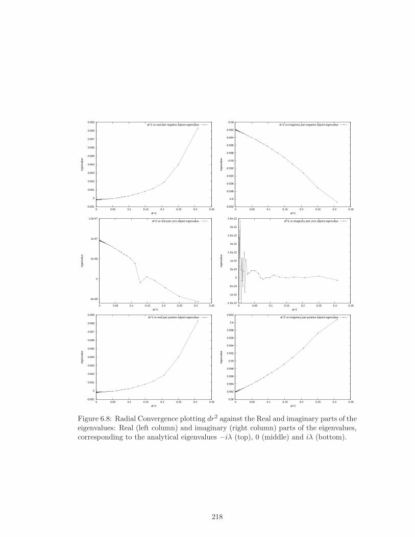
-0.001
0
0.001
0.002
0.003
0.004
0.005
0.006
0.007
0.008
0.009
0 0.05 0.1 0.15 0.2 0.25 0.3 0.35
eige
nval
ue
dr^2
dr^2 vs real part negative adjoint eigenvalue
-0.602
-0.6
-0.598
-0.596
-0.594
-0.592
-0.59
-0.588
-0.586
-0.584
-0.582
-0.58
0 0.05 0.1 0.15 0.2 0.25 0.3 0.35
eige
nval
ue
dr^2
dr^2 vs imaginery part negative adjoint eigenvalue
-5e-08
0
5e-08
1e-07
1.5e-07
0 0.05 0.1 0.15 0.2 0.25 0.3 0.35
eige
nval
ue
dr^2
dr^2 vs real part zero adjoint eigenvalue
-1.5e-22
-1e-22
-5e-23
0
5e-23
1e-22
1.5e-22
2e-22
2.5e-22
3e-22
3.5e-22
0 0.05 0.1 0.15 0.2 0.25 0.3 0.35
eige
nval
ue
dr^2
dr^2 vs imaginery part zero adjoint eigenvalue
-0.001
0
0.001
0.002
0.003
0.004
0.005
0.006
0.007
0.008
0.009
0 0.05 0.1 0.15 0.2 0.25 0.3 0.35
eige
nval
ue
dr^2
dr^2 vs real part positive adjoint eigenvalue
0.58
0.582
0.584
0.586
0.588
0.59
0.592
0.594
0.596
0.598
0.6
0.602
0 0.05 0.1 0.15 0.2 0.25 0.3 0.35
eige
nval
ue
dr^2
dr^2 vs imaginery part positive adjoint eigenvalue
Figure 6.8: Radial Convergence plotting dr2 against the Real and imaginary parts of theeigenvalues: Real (left column) and imaginary (right column) parts of the eigenvalues,corresponding to the analytical eigenvalues −iλ (top), 0 (middle) and iλ (bottom).
218
6.7 Conculsion
To conclude, we have seen that evcospi is a very versatile and useful tool in the
study of the response functions of spiral waves. We have seen that the convergence
testing of the program indicates that the program is running as it should and that the
numerical methods used have been implemented correctly into the code.
We have also seen that EZ-Freeze can be used to generate initial conditions for
evcospi. These are produced very quickly and also very accurately. They are generated
in a format which is in the evcospi “own” format, meaning that the evcospi.
This work is currently ongoing and we hope that the program will be made available
very soon for other researchers to use. The program will also be extended to look at
the response functions for scroll waves.
219
Chapter 7
Conclusions & Further Work
The main results from this work are:
• A theory of drift of spiral waves using the method of quotient system by the
special Euclidean group is developed.
• Our new theory has been applied to the drift of rigidly rotating spirals and the
results are consistent with those produce by earlier theories.
• Our new theory has been applied to the drift of meandering spirals for which there
has been no complete theory earlier. The theory predicts the drift of meandering
spirals and also a possibility of phase locking between external stimulation and
meandering, which has been observed experimentally.
• The method of quotient system by the special Euclidean group has been im-
plemented numerically (EZ-Freeze program). The numerical convergence of this
method has been demonstrated.
• The numerical implementation of the method of quotient system can be used to
study drift of spiral waves on indefinitely long time intervals.
• The numerical implementation of the method of quotient system has been used
to investigate the behaviour of the spiral waves near the “large core” boundaries,
which are difficult to study by standard methods. It has been demonstrated that
the new method can distinguish between different theoretical asymptotics.
• The numerical implementation of the method of quotient system has been used to
investigate the behaviour of the spiral waves near the “l:1 resonance” parametric
line. It has been demonstrated that the behaviour of the quotient system does
not demonstrate any peculiarities across this line.
220
• The numerical implementation of the method of quotient system has been used to
generate rigidly rotating spiral wave solutions in the format suitable for the use
in evcospi, a program for calculation of the response functions of spiral waves.
• Numerical convergence of the solutions obtained by evcospi has been demon-
strated.
Future directions for this work include:
• Extend our theory to include at least O(ǫ2) terms to see if frequency locking can
be detected. Also, studying locking in FHN model.
• Use EZ-Freeze to investigate frequency locking.
• Asymptotic investigation of the behaviour of the solutions after the critical point
when studying large core spirals.
• Investigation into the shape of the limit cycles of the drifting and meandering
spiral spiral waves and how the behaviour of the spiral wave is dependent on the
shape of the limit cycles.
• Investigating further the numerical evidence of a Hopf bifurcation from rigid
rotation to meander by using EZ-Freeze to study the amplitude of the limit cycles.
• Another interesting line of research would be to see how our theory could be
adapted to three dimensional scroll waves.
221
Appendix A
Definitions
Throughout this thesis, we will be using particular words and phrases. It is assumed
that the reader will have no specific knowledge of these terms and therefore we introduce
some basic definitions for the reader’s perusal.
A.1 Dynamical System
Although not specifically mentioned in this thesis, the definition of a Dynamical
System should be known as the systems studied throughout this report are indeed
Dynamical Systems. A Dynamical System is a pair X,φt, where X is a state space
and φt : X → X is a family of evolution operators satisfying the conditions φ0 = id
and φt+s = φt φs. A State Space is a set containing all possible states of the system
[6].
The most common way to represent a continuous-time dynamical system is with a
set of differential equations.
A.2 Quasiperiodicity
Meandering waves display quasiperiodic motion. Quasiperiodic motion is a regular
but non-chaotic motion which consists of a combination of period motions with a tra-
jectory that after a sufficient period of time pass arbitrarily close to an earlier value,
but never on it.
A dynamical system is called k-quasi-periodic if it can be written in the form:
x(t) = f(ω1t, ω2t, .., ωkt)
where ωi for i = 1, .., k are such that they are not rationally related, i.e. the relationship
222
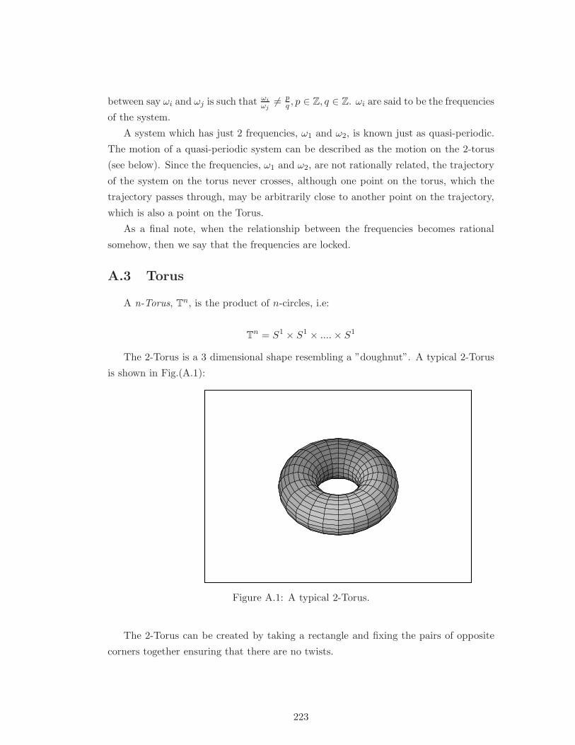
between say ωi and ωj is such that ωi
ωj6= p
q, p ∈ Z, q ∈ Z. ωi are said to be the frequencies
of the system.
A system which has just 2 frequencies, ω1 and ω2, is known just as quasi-periodic.
The motion of a quasi-periodic system can be described as the motion on the 2-torus
(see below). Since the frequencies, ω1 and ω2, are not rationally related, the trajectory
of the system on the torus never crosses, although one point on the torus, which the
trajectory passes through, may be arbitrarily close to another point on the trajectory,
which is also a point on the Torus.
As a final note, when the relationship between the frequencies becomes rational
somehow, then we say that the frequencies are locked.
A.3 Torus
A n-Torus, Tn, is the product of n-circles, i.e:
Tn = S1 × S1 × ....× S1
The 2-Torus is a 3 dimensional shape resembling a ”doughnut”. A typical 2-Torus
is shown in Fig.(A.1):
Figure A.1: A typical 2-Torus.
The 2-Torus can be created by taking a rectangle and fixing the pairs of opposite
corners together ensuring that there are no twists.
223
A.4 Bifurcations
In laymans terms, a bifurcation point separates regions of stability in a particular
system. Consider for example the following simple system of ODE’s:
x = −x + y
y = ax− y
The system has a fixed point at the origin, (0,0), and the stability matrix at this
point, J(0,0), is given by:
J(0, 0) =
(
−1 1a −1
)
Eigenvalues are therefore the solution to the equation λ2+2λ+(1+a) = 0 ⇒ λ± =
−1±√−a. Therefore, we can come to the following conclusions about the stability of
the fixed point (0,0):
if a < −1 ⇒ λ± have opposite signs ⇒ Saddle Point - Unstableif − 1 < a ≤ 0 ⇒ λ± are both negative ⇒ Stable Node
if a > 0 ⇒ λ± are complex with a positive real part ⇒ Stable Focus Point
We therefore say that there is a Bifurcation when a=-1, at which point the system
goes from unstable to stable.
This is a very simple example of a system possessing a Bifurcation point. There
are many different types of bifurcations (Fold, Pitchfork, Neimark-Sacker, Hopf, Hopf-
Hopf) but the ones that we are most interested in are the Hopf Bifurcations and also the
Neimark-Sacker Bifurcations (sometimes referred to as a Secondary Hopf Bifurcation).
A.4.1 Hopf Bifurcation
A Hopf Bifurcation occurs when a fixed point of the system in question goes from
being stable to being unstable and is surrounded by a stable limit cycle. The Hopf
Bifurcation point is the point at which the complex eigenvalues of the system at the
fixed point in question cross the imaginary axis. Hence, the eigenvalues of the system
are purely imaginary at the Hopf Bifurcation Point. The eigenvalue equation may be
written in the form:
λ2 + Tr(J)λ + Det(J) = 0
224
where Tr(J) is the trace of the Jacobian and Det(J) is the determinant of the
Jacobian. Hence, sufficient conditions for the presence of a Hopf bifurcation is Tr(J) =
0 and Det(J) > 0, giving the eigenvalues to be λ± = ±i√
Det(J).
A.4.2 Supercritical and Subcritical Hopf Bifurcations
A Supercritcial Hopf Bifurcation is one in which the limit cycle is attracting, i.e it
is a stable limit cycle. Therefore, a Subcritical Hopf Bifurcation is one in which the
limit is repelling, i.e. unstable.
A.4.3 Hopf Bifurcation Normal Form
In this section we provide a brief but thorough review of the Hopf Bifurcation and
how it applies to our system and spiral wave solution.
Consider the following dynamical system:
x = f(x, p), x ∈ Rm, x = (x1, x2, . . . , xm) (A.1)
This system has an equilibrium at x∗, satisfying:
0 = f(x∗, p)
Now the right hand side of (A.1), has both linear and non-linear parts. In order
to study the full system inclusive of the non-linear parts, we need to use the Center
Manifold Theorem (this will be introduced later on). Therefore, we need our equilibrium
to located at the origin. Let us introduce a change of coordinates:
y = x− x∗
Therefore, our original system now becomes:
y = g(y, p), y ∈ Rm, y = (y1, y2, . . . , ym)
The equilibrium of this new system is now located at the origin, since if at the
equilibrium x = x∗, then y = 0 at the equilibrium:
0 = g(0, p)
The Hopf Bifurcation Theory (see [42]) tells us that if a system possesses a Hopf
Bifurcation, then there are 2 complex conjugate eigenvalues that lie on the imaginary
axis when the Hopf Bifurcation takes place. Also, the real parts of these eigenvalues
are monotonic functions of the system parameter. If the real parts are monotonically
225
increasing, then we get a Supercritical Hopf Bifurcation. If the real parts are monoton-
ically decreasing, then we get a Subcritical Hopf Bifurcation. This then leads to limit
cycle solutions being observed in the system.
Let us consider the linear part of the system and assume that the system has
eigenvalues in the following form:
λ1,2 = ǫ(p)± iω(p), Reλi≥3 < 0
Now, ǫ(p) is a monotonic function. Let us assume that it is monotonically increasing.
This means that ǫ(p) has an inverse. In particular this inverse is p = p(ǫ). Therefore,
we have:
y = g(y, ǫ), y ∈ Rm, y = (y1, y2, . . . , ym) (A.2)
λ1,2 = ǫ± iω(ǫ)
Another restriction that we have with the Center Manifold Theorem is that the
system studied must be independent of parameters. System (A.2) is clearly dependent
on parameter ǫ. So how can be make this system independent of parameters? One
way is to make ǫ a dynamical variable of the system. We know that the parameters
of our system stay constant for all time and therefore we can introduce the following
conditions:
y = g(y, ǫ)
ǫ = 0
If we let u = (y, ǫ)T , then we get a new parameter independent system:
u = h(u), u ∈ Rm+1, u = (u1, u2, . . . , um) (A.3)
Let us think about an equilibrium point of this system. Let us suppose this equi-
librium point is at u∗:
u∗ =
(
y∗
ǫ
)
=
(
0ǫ
)
This means that we have an infinite amount of equilibrium points. However, as
we stated earlier, the Center Manifold Theorem insists that the equilibrium is at the
226
origin. Hence, we must have ǫ = 0. Also, this means that in the linear system, we have
that ǫ = 0.
Let us now split the right hand side of (A.3) into its linear and non-linear parts:
u = Ju + N(u), N(u) = O(u2) (A.4)
where J is the Jacobian of the system. Firstly, let us neglect the non-linear terms and
look at the linear system:
u = Ju
The Jacobian is an (m + 1)× (m + 1) matrix and is given by:
J =
(
∂g∂y
0
0 0
)
The eigenvalues are exactly the same as those in the system (A.2) but with an extra
eigenvalue λ0 = 0. Therefore the eigenvalues are:
λ0 = 0, λ1,2 = ±iω0, Reλi≥3 < 0
remembering that ǫ = 0 and also denoting ω(0) = ω0. If we denote the corresponding
eigenvectors as vi for i = 0, . . . ,m, then the solution in the linearised system is:
u =m∑
i=0
aivieλit
= a0v0eλ0t + a1v1e
λ1t + a2v2eλ2t +
m∑
i=3
aivieλit
= a0v0 + a1v1eiωt + a1v1e
−iωt +
m∑
i=3
aivieλit
noting that because λ2 = λ1 ⇒ v2 = v1, then a2 = a1 for our solution to produce
real results. What happens as t → ∞? We can see that since Reλi≥3 < 0, then∑m
i=3 aivieλit → 0. Therefore, over the long term, our solution becomes:
u = a0v0 + a1v1eiωt + a1v1e
−iωt
Now, all solutions to the linear system lie on a Center Subspace. The Center Sub-
space is a subspace of space of solutions that is spanned by the eigenvectors of the
227
linearised system. In the following subsection we show an example this statement.
Also, the solutions to the linear system can be expressed as a linear combination of the
eigenvectors - this is known as the span of the system:
u = α0v0 + α1v1 + α1v1|α = (α0, α1, α1) (A.5)
So, any solution on this Center Subspace can be expressed in terms of α, i.e. α is
the coordinate of a solution lying on the Center Subspace. Also, the Center Subspace
is such that any solution that does not lie on it is attracted to it over time. This is due
to the “discarded” terms∑m
i=3 aivieλit, which actually do not actually vanish but are
extremely small. We also note that if the solution is on the Center Subspace, then it
will stay in it indefinitely. It can also be seen that as we move through time, we get
different values of α. Therefore, we can say that α is dependent on time.
We now bring back the non-linear terms. In order for us to study the full system
inclusive of the non-linear terms, we must use the Center Manifold Theorem.
Theorem A.4.1 (Center Manifold Theorem (CMT)). Given the parameter indepen-
dent system (A.4), then there exists a Center Manifold which is:
1. tangential at the origin,
2. invariant,
3. attracting.
In our system we have u ∈ Rm+1. If we want to study our system in the region of
the equilibrium, then the CMT allows us to study our full system in a reduced system
consisting of k ODE’s, where k is the number of eigenvalues with zero real part. In our
case, we have 3 eigenvalues with zero real part and hence the CMT implies that we will
have 3 ODE’s describing the motion of the system near the equilibrium point.
So how does the CMT allow this? Well, let us consider the CMT. Firstly, what does
point 3 in Theorem (A.4.1) tells us that any solution to our system which does not start
on the Center Manifold will be attracted to the Center Manifold, but the trajectory
will not be part of the manifold. This is evident in our system since Reλ1,2 < 0, and
therefore over time these will decay to zero. Therefore, we can model the motion using
just 3 equations in our.
The second point in the theorem states that any trajectory starting on the Center
Manifold will remain on the manifold indefinitely. Hence, we model the system using
a system of closed ODE’s.
Finally, the first point in the theorem states that in region sufficiently close to
the origin, i.e. the equilibrium, there is a one to one correspondence between points
228
on the Center Manifold and points on the Center Subspace. Therefore, in the region
of the equilibrium, we can model the motion of the system as motion on the Center
Subspace. Therefore, each point on the trajectory of a solution to our system will have
the coordinates α = (α0, α1, α1). Accordingly, the 3 ODE’s that will model this motion
will be:
α0 = k0(α)
α1 = k1(α)
˙α1 = k2(α)
Now let us now return to our problem. We saw that we could express the solution
in the linear system as the span of the eigenvectors (A.5). The CMT implies that the
solution in the full system may also be expressed in this form. Let us now substitute
(A.5) into (A.4):
u = Ju + N(u)
α0v0 + α1v1 + ˙α1v1 = α0Jv0 + α1Jv1 + α1J v1 + N(α))
Considering just the linear terms and using Jvi = λivi, we get:
α0v0 + α1v1 + ˙α1v1 = α0λ0v0 + α1λ1v1 + α1λ1v1
Equating coefficients of the eigenvalues, we get:
α0 = α0λ0
α1 = α1λ1
˙α1 = α1λ1
not adding in the non-linear terms and substituting in the expressions for the eigenval-
ues we get:
α0 = 0 + N0(α) (A.6)
α1 = iω0α1 + N1(α) (A.7)
˙α1 = −iω0α1 + N2(α) (A.8)
Let us consider (A.6). We know that u is of the form:
229
u = α0v0 + α1v1 + α1v1
⇒(
yǫ
)
= α0
(
01
)
+ α1
(
...0
)
+ α1
(
...0
)
Therefore, α0 = ǫ⇒ α0 = ǫ = 0. Therefore, we have 0 = N0(u).
Let us now consider (A.7). We can also consider (A.8) at the same time since it is
just the conjugate of (A.7). Using Taylor’s Expansion, we can expand the non-linear
terms and get:
α1 = iω0α1 + Aα20 + Bα2
1 + Cα21 + Dα0α1 + Eα0α1 + Fα1α1 + O(α3)
Firstly, note that α0 = ǫ and iω0 = λ1. Also, in our system, we are denoting the
motion of the solutions as lying on the Center Subspace. Therefore we have that ǫ = 0.
This means that:
α1 = (Dǫ + iω0)α1 + Eǫα1 + Aǫ2 + Bα21 + Cα2
1 + Fα1α1 + O(α3)
= λ1α1 + Bα21 + Cα2
1 + Fα1α1 + O(α3)
We now make a Poincare change of variables using:
α1 = w + p1w2 + p2ww + p3w
2 + O(|w|3) (A.9)
Therefore, we can say that w is given by the inverse of α1:
w = α1 − p1α21 − p2α1α1 − p3α
21 + O(|α1|3) (A.10)
This can be seen by substituting (A.10) into (A.9) which will give, to O(|α1|3),α1 = α1 + O(|α1|3). Differentiating with respect to time:
w = α1 − 2p1α1α1 − p2(α1α1 + α1 ˙α1)− 2p3α1 ˙α1
= (λ1α1 + Bα21 + Cα2
1 + Fα1α1)− 2λ1p1α21 − p2(λ1α1α1 + λ1α1α1)− 2λ1p3α
21
= λ1α1 + α21(B − 2p1λ1) + α1α1(F − p2(λ1 + λ1)) + α2
1(C − 2p3λ1)
= λ1(w + p1w2 + p2ww + p3w
2) + w2(B − 2p1λ1) + ww(F − p2(λ1 + λ1))
+w2(C − 2p3λ1)
= λ1w + w2(B − p1λ1) + ww(F − p2λ1) + w2(C − p3(2λ1 − λ1))
230
omitting all higher order terms. We can see that we can eliminate all quadratic terms
by setting:
p1 =B
λ1
p2 =F
λ1
p3 =C
2λ1 − λ1
We also see that the denominators in the above expressions for p1 to p3 are never
zero since ω0 > 0. We therefore have:
w = λ1w + O(|z|3) (A.11)
Let us now look at the cubic terms and express (A.11) as follows:
w = λ1w + Gw3 + Hw2w + Kww2 + Lw3 + O(|w|4)
We now make another Poincare Change of Variables:
w = z + q1z3 + q2z
2z + q3zz2 + q4z3 (A.12)
⇒ z = w − q1w3 − q2w
2w − q3ww2 − q4w3 + h.o.t. (A.13)
Differentiating (A.13) with respect to time gives us:
z = w − 3q1w2w − q2(2www + w2 ˙w)− q3(ww2 + 2ww ˙w)− 3q4w
2 ˙w
= (λ1w + Gw3 + Hw2w + Kww2 + Lw3)− 3q1λ1w3 − q2(2λ1w
2w
+λ1w2w)− q3(λ1ww2 + 2λ1ww2)− 3q4λ1w
3
= λ1w + w3(G− 3q1λ1) + w2w(H − q2(2λ1 + λ1))
+ww2(K − 2q3λ1) + w3(L− q4(3λ1 + λ))
= λ1(z + q1z3 + q2z
2z + q3zz2 + q4z3) + z3(G− 3q1λ1)
+z2z(H − q2(2λ1 + λ1)) + zz2(K − 2q3λ1) + z3(L− q4(3λ1 + λ)) + O(|z|4)= λ1z + z3(G− 2q1λ1) + z2z(H − q2(λ1 + λ1))
+zz2(K − q3(2λ1 − λ1)) + z3(L− 3q4λ1)
In order to eliminate the cubic terms we require the following to be true:
231
q1 =G
2λ1
q2 =H
λ1 + λ1
q3 =K
2λ1 − λ1
q4 =L
3λ1
We see that the expression for q2 cannot be true since if λ1 = iω0 then λ1 + λ1 = 0.
Therefore, the denominator for q2 is zero. Hence, we can eliminate all cubic terms apart
from the z2z = z|z|2 term. Further analysis shows that for higher order terms (i.e.
O(|z|4)), all terms can actually cancel out. Therefore, we are left with the following,
which is the Hopf Normal Form:
z = λ1z + q2z|z|2
where z is, in fact, a limit cycle solution. Let us now work our way back to the original
system. We know that the solution to (A.3) is:
u = α0v0 + α1v1 + α1v1 + O(|α1|3)
In the system given by (A.2), the solution will then be:
y = α1w1 + α1w1 + O(|α1|3)
and in the first system:
x = x∗ + α1w1 + α1w1 + O(|α1|3) (A.14)
Finally, we note that α1 = z + O(|z|3) and therefore we get that (A.14) can be
expressed as:
x = x∗ + zw1 + zw1 + O(|z|3) (A.15)
All we now need to do is apply this to our spiral wave solutions. We know that in
our system (2.23) the solutions generated are of the form v, c, ω. This is infact our
x in (A.15).
232
vcω
=
v∗
c∗ω∗
+ z
wv
wc
wω
+ z
wv
wc
wω
+ h.o.t.
Therefore we now have expressions for c = (cx, cy) and ω:
cx = cx∗ + zcx1 + zcx1 + O(|z|3)cx = cy∗ + zcy1 + zcy1 + O(|z|3)ω = ω∗ + zω1 + zω1 + O(|z|3)
A.5 Codimension (Codim)
Codimesion, or Codim as it is sometimes referred to as, is basically the difference
in the dimensions of 2 comparing spaces or manifolds. Let X be a vector space of
dimension a, and Y a sub space of X, i.e. Y ⊂ X, of dimension b. Then X is said to
have Codim = a− b.
As an example, take the Poincare Cross Section of a 2-Torus. The 2-Torus has
Dim=3 and the Poincare Cross Section has Dim=2. Hence, the Codim of the Torus is
1. Another way to look at this is that we have to introduce just one restriction to the
2-Torus in order to reduce its dimension to 2 - hence the Codim is 1.
A.6 Excitability
A system is classed as Excitable and displays Excitability if it is capable of generating
a wave of some description and supporting its propagation. Cardiac tissue is classed as
an excitable media since it is capable of supporting the propagation of waves. Consider
Fig.(A.2):
Now, if the wave front is moving in the direction shown for increasing time, i.e. in
the positive x-direction, then this shows that the wave is propagating. If the wave is
moving in the opposite direction for increasing time then the wave is not propagating
but is decaying. Hence, we require that for a system to display excitability, then the
wave front must move in the positive x-direction as shown.
A.7 Euclidean Symmetry
A system is said to be invariant under under Euclidean Symmetry if it possesses
the properties of a Symmetry Group and obeys Euclidean Symmetry laws. We will
throughout this report consider only the 2 dimensional Euclidean Group, SE(2), pos-
sessing the following properties:
233
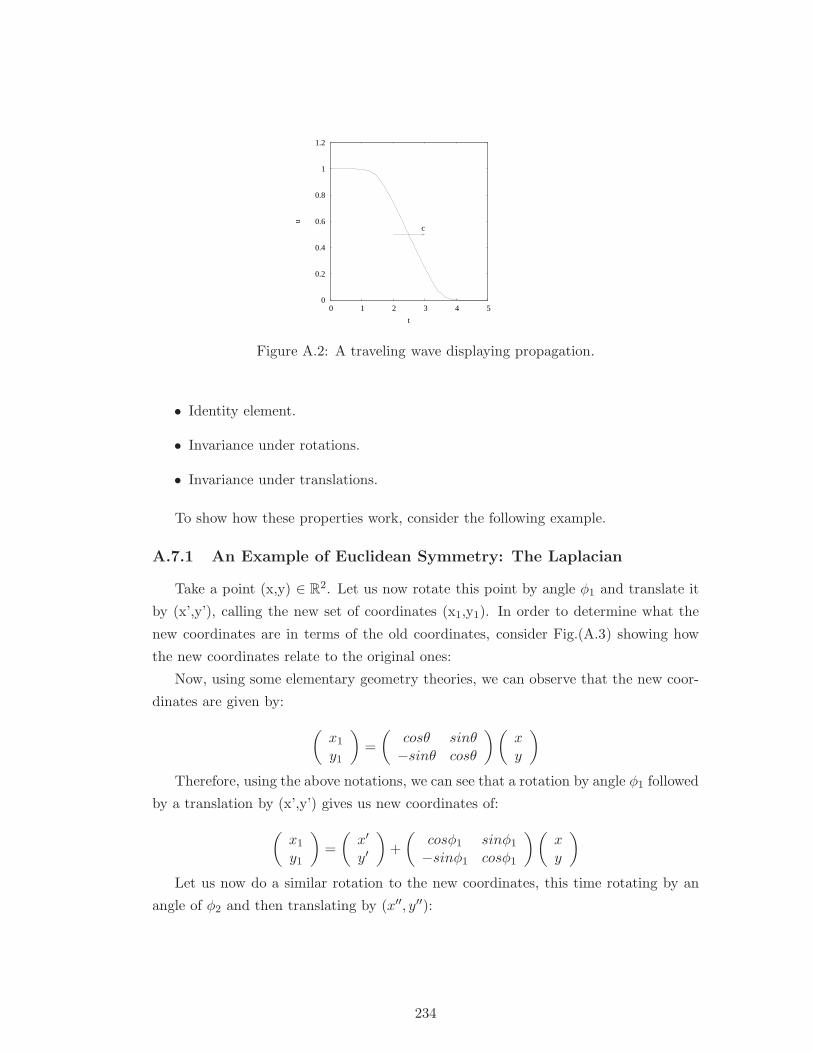
0
0.2
0.4
0.6
0.8
1
1.2
0 1 2 3 4 5
u
t
c
Figure A.2: A traveling wave displaying propagation.
• Identity element.
• Invariance under rotations.
• Invariance under translations.
To show how these properties work, consider the following example.
A.7.1 An Example of Euclidean Symmetry: The Laplacian
Take a point (x,y) ∈ R2. Let us now rotate this point by angle φ1 and translate it
by (x’,y’), calling the new set of coordinates (x1,y1). In order to determine what the
new coordinates are in terms of the old coordinates, consider Fig.(A.3) showing how
the new coordinates relate to the original ones:
Now, using some elementary geometry theories, we can observe that the new coor-
dinates are given by:
(
x1
y1
)
=
(
cosθ sinθ−sinθ cosθ
)(
xy
)
Therefore, using the above notations, we can see that a rotation by angle φ1 followed
by a translation by (x’,y’) gives us new coordinates of:
(
x1
y1
)
=
(
x′
y′
)
+
(
cosφ1 sinφ1
−sinφ1 cosφ1
)(
xy
)
Let us now do a similar rotation to the new coordinates, this time rotating by an
angle of φ2 and then translating by (x′′, y′′):
234
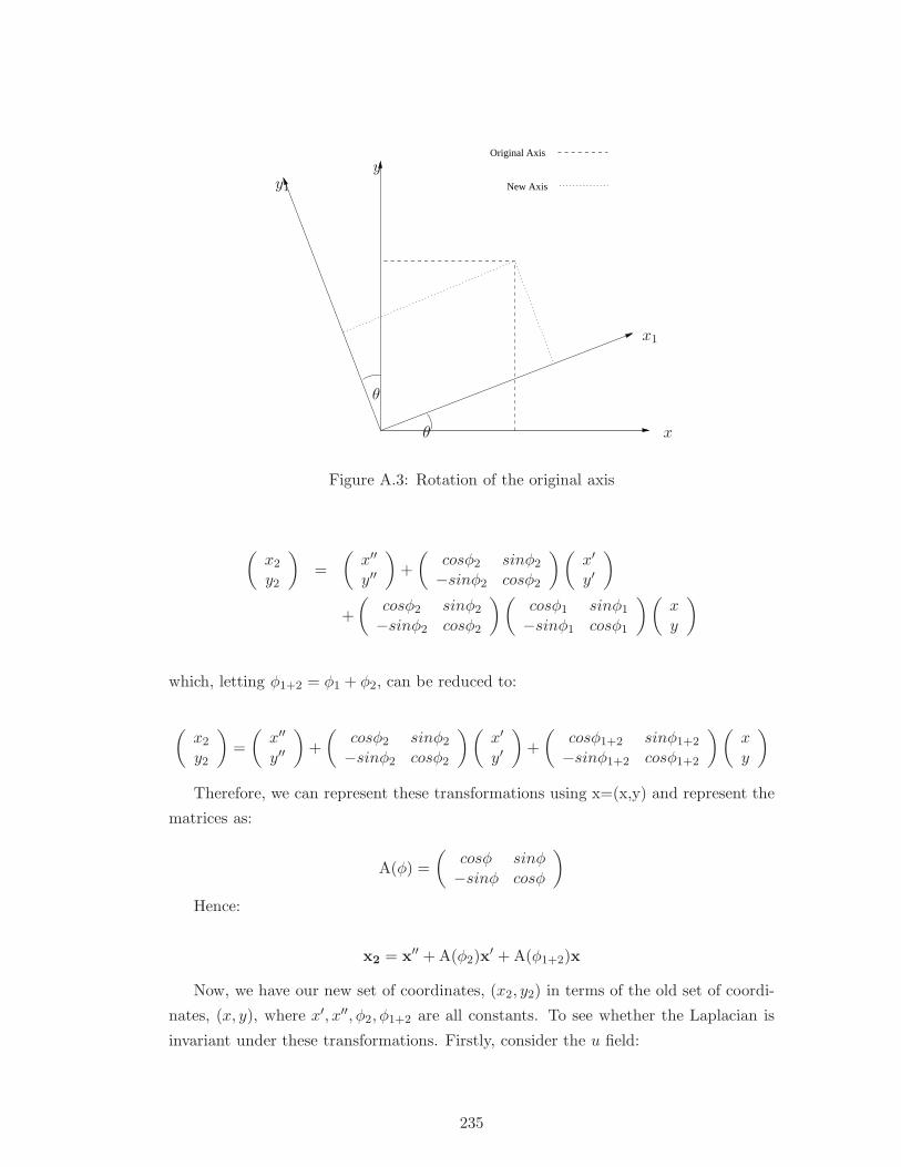
Original Axis
New Axisy1
y
x1
xθ
θ
Figure A.3: Rotation of the original axis
(
x2
y2
)
=
(
x′′
y′′
)
+
(
cosφ2 sinφ2
−sinφ2 cosφ2
)(
x′
y′
)
+
(
cosφ2 sinφ2
−sinφ2 cosφ2
)(
cosφ1 sinφ1
−sinφ1 cosφ1
)(
xy
)
which, letting φ1+2 = φ1 + φ2, can be reduced to:
(
x2
y2
)
=
(
x′′
y′′
)
+
(
cosφ2 sinφ2
−sinφ2 cosφ2
)(
x′
y′
)
+
(
cosφ1+2 sinφ1+2
−sinφ1+2 cosφ1+2
)(
xy
)
Therefore, we can represent these transformations using x=(x,y) and represent the
matrices as:
A(φ) =
(
cosφ sinφ−sinφ cosφ
)
Hence:
x2 = x′′ + A(φ2)x′ + A(φ1+2)x
Now, we have our new set of coordinates, (x2, y2) in terms of the old set of coordi-
nates, (x, y), where x′, x′′, φ2, φ1+2 are all constants. To see whether the Laplacian is
invariant under these transformations. Firstly, consider the u field:
235
∂u
∂x=
∂u
∂x2
∂x2
∂x+
∂u
∂y2
∂y2
∂x
⇒ ∂u
∂x= cos(φ1+2)
∂u
∂x2− sin(φ1+2)
∂u
∂y2
⇒ ∂2u
∂x2= cos2(φ1+2)
∂2u
∂x22
+ sin2(φ1+2)∂2u
∂y22
Similarly, for the second derivative of u with respect to y, we get:
∂2u
∂y2= sin2(φ1+2)
∂2u
∂x22
+ cos2(φ1+2)∂2u
∂y22
Therefore, the Laplacian is given by:
∆u =∂2u
∂x2+
∂2u
∂y2
⇒ ∆u = (cos2(φ1+2)∂2u
∂x22
+ sin2(φ1+2)∂2u
∂y22
) + (sin2(φ1+2)∂2u
∂x22
+ cos2(φ1+2)∂2u
∂y22
)
⇒ ∆u =∂2u
∂x22
+∂2u
∂y22
⇒ ∆u = ∆u2
where u2 = u(x2, y2). Hence we can conclude that the Laplacian is invariant under
the actions of an SE(2) group.
A.8 A Bit of Group Theory
The information that follows has been taken from various references - [45], [33], and
[32]
A.8.1 Definition
A group is defined to be a set of elements, G, together with an operation, , which
obey the following axioms:
1. Closure - ∀g, h ∈ G then g h ∈ G.
2. Associativity - ∀f, g, h,∈ G then (f g) h = f (g h)
3. Identity - ∀g ∈ G ∃ e ∈ G such that g e = g
4. Inverse - ∀g ∈ G ∃ h ∈ G such that g h = e
236
A further axiom is Commutativity which states:
∀g, h ∈ G, g h = h g
A group obeying this axion is said to be an Abelian Group.
A.8.2 Invariance and Equivariance
If g ∈ G and x ∈ X is a set of solutions to a particular equation (in our case
we would be looking at the set of all solutions u = u(r, t) = (u1, u2, ..) ∈ Rl to the
Reaction-Diffusion system of equations, then we say that a solution x′ ∈ X is invariant
if:
x′ = g · x
i.e. x is a solution and x′ is a solution which is derived by applying the action of a
group element g ∈ G to the original solution, x. We say that “solutions x ∈ X are
invariant under action of g ∈ G”.
Let Y,Z ⊂ G and define a map f : Y 7→ Z. Then we say that f is equivariant if:
f(gy) = gf(y) y ∈ Y
A.8.3 Direct Product
Let (G, G) and (H, H) be groups. The the direct product between these groups
are:
G×H = (g, h)|g ∈ G,h ∈ H
A.8.4 Orbit
The Orbit of an element x ∈ X, is the set of all possible transformations of x under
the action of group elements which belong to the set X:
Gx = g · x|x ∈ X, g ∈ G
A.8.5 Stabiliser
The Stabiliser of x ∈ X is defined as:
Gstab = g · x = x|x ∈ X, g ∈ G
The stabiliser is sometimes often referred to as the Isotropy Subgroup.
237
A.8.6 Centre
The center of a group G is defined to be:
C(G) = t ∈ G|tg = gt ∀g ∈ G
Therefore, in this case, we are looking at an Abelian Group (see above).
A.8.7 Normaliser
The Normaliser of a subgroup H ⊂ G is defined as:
NG(H) = g ∈ G : gHg−1 = H
A.8.8 Normal and Quotient Groups
We say that a subgroup H ⊂ G is a normal subgroup if it is invariant under action
of elements of G:
N G = ∀g ∈ G : gHg−1 = H
If N is a normal subgroup then we define the Quotient group to be the set of all
left cosets of N in G and is denoted by G/N .
A.8.9 Euclidean Groups - E(2), SE(2), SO(2) and Z(2)
The Euclidean Group, E(2), if the 2 dimensional group consisting of all rotations,
translations and reflections. A subgroup E(2) is the group of rotations and translation,
SE(2), which has 2 further subgroups - the group of rotations, SO(2), and the group
of translations, R2. Note that E(n) is the Euclidean group in n dimensions.
(SO(2) ∪ R2) ⊂ SE(2) ⊂ E(2)
Group action on a solution u(r, t)
In this subsection, we show that the following is true:
T (g)u(r, t) = u(g−1r, t)
Firstly, consider the 1-dimensional case r = x. In Fig.(A.4)), have u(x) being
moved parallel to the x-axis in the positive direction, i.e. we start at x1 and shift it to
x1 + X = x2, where X = x2 − x1. We have a solution u(x), denoted in Fig.(A.4) by
the solid line, and this solution is shifted in the positive x direction via a group action,
i.e. T (g)u(x) = u(x).
238
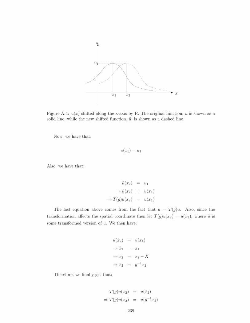
x1 x2
u
x
u1
Figure A.4: u(x) shifted along the x-axis by R. The original function, u is shown as asolid line, while the new shifted function, u, is shown as a dashed line.
Now, we have that:
u(x1) = u1
Also, we have that:
u(x2) = u1
⇒ u(x2) = u(x1)
⇒ T (g)u(x2) = u(x1)
The last equation above comes from the fact that u = T (g)u. Also, since the
transformation affects the spatial coordinate then let T (g)u(x2) = u(x2), where u is
some transformed version of u. We then have:
u(x2) = u(x1)
⇒ x2 = x1
⇒ x2 = x2 −X
⇒ x2 = g−1x2
Therefore, we finally get that:
T (g)u(x2) = u(x2)
⇒ T (g)u(x2) = u(g−1x2)
239
Similar arguments can be arranged for the 2 dimensional case and it can be shown
that the following is true for g ∈ SE(2):
T (g)u(r, t) = u(g−1r, t)
Invariance Properties
In their 1996 paper, Biktashev et al considered the symmetry with respect to the
Special Euclidian Group, SE(2), i.e. the group of rotations and translations. It can
be shown that spiral wave solutions are actually invariant under actions from SE(2).
That is, if we take a spiral, rotate and move it to a different position within the domain
in which it is rotating, then we will still have a spiral wave solution only in a different
position and phase. We prove this in the following paragraphs.
Let assume that we have a Reaction Diffusion Equation:
∂tu = D∇2u + f(u) (A.16)
with u = u(x, y, t) and u ∈ R2. Let us assume that the solution, u, to this equation,
now undergoes an action of the the group element g ∈ SE(2):
u = T (g)u(x, y, t) = u(g−1x, g−1y, t) = u(x, y, t)
If we let the group element be a rotation followed by a translation, i.e. g = R, θwhere θ is the angle of rotation and R = (X,Y ) is the translation vector, then we
have that g−1 = −θ,−R, i.e. a translation (in the opposite direction, followed by a
rotation:
(
xy
)
=
(
cos θ sin θ− sin θ cos θ
)(
x−Xy − Y
)
⇒ x = (x−X) cos θ + (y − Y ) sin θ
and y = −(x−X) sin θ + (y − Y ) cos θ
Let us now assume that u is a solution to (A.16):
∂tu = D∇2u + f(u)
Consider the right hand side of (A.8.9). Eqn.(A.8.9) gives us:
∂u
∂t=
∂u
∂t
240
since the transformation applied only affects the spatial variables and not the temporal
ones. Consider now the Laplacian terms:
∇2u =∂2u
∂x2+
∂2u
∂y2
Now, consider just the differentiation with respect to x:
∂u
∂x=
∂u
∂x
∂x
∂x+
∂u
∂y
∂y
∂x
= cos θ∂u
∂x+ sin θ
∂u
∂y
Differentiating again with respect to x:
∂2u
∂x2= cos2 θ
∂2u
∂x2+ sin2 θ
∂2u
∂y2
Similar calculations yield:
∂2u
∂y2= sin2 θ
∂2u
∂x2+ cos2 θ
∂2u
∂y2
Hence the Laplacian for u is given by:
∇2u = (cos2 θ∂2u
∂x2+ sin2 θ
∂2u
∂y2) + (sin2 θ
∂2u
∂x2+ cos2 θ
∂2u
∂y2)
= (cos2(θ) + sin2(θ))∂2u
∂x2+ (cos2(θ) + sin2(θ))
∂2u
∂y2
=∂2u
∂x2+
∂2u
∂y2
= ∇2u
Finally, consider the function f(u):
f(u) = f(u((x, y, t)))
= f(u((x−X) cos θ + (y − Y ) sin θ,−(x−X) sin θ + (y − Y ) cos θ, t))
= f(u(x, y, t))
= f(u)
So, putting all our results together gives us:
241
∂tu = D∇2u + f(u)
⇒ ∂tu = D∇2u + f(u)
Hence, we can conclude that the Reaction Diffusion Equation is invariant under
Euclidean Symmetry.
A.9 Manifolds
A.9.1 Definition
A Manifold is an Euclidean Space of solutions which has codimension k and also
members of a Topological Space (the original space) are mapped into this Euclidean
Space. It is in affect, a represention of the original solutions but in a space of lower
dimension.
In group theoretical terms, a Manifold can be represented as a Quotient Group (see
above):
M = Gx|x ∈ X = X/G
A.9.2 Simple Examples
The circle in R2
Consider the circle as shown in Fig.(A.5). A small arc on this circle can be represent
as a line provided that the arc (neighbourhood) is small enough. Therefore, we can
represent a neighbourhood in R2 as a straight line in R. Therefore our manifold, the
straight line, has codim-1, reducing our original space from 2 dimensions to 1 dimension.
Group of rotations about the origin
Consider all possible rotations about the origin in R2. If we take a point (x, y) ∈ R
2,
then this would belong to one of the circles as shown in Fig.(A.6). Therefore, every
point in R2 belongs to one of these circles.
Therefore, if we know a point on a particular circle we can determine all other points
on that circle by applying all rotations to that point. So, all we need to determine all
possible points on a circle is one single point. We can do this for all other circles and
therefore we get a line of solutions as shown in Fig.(A.6). This line is a manifold of
codim-1.
242
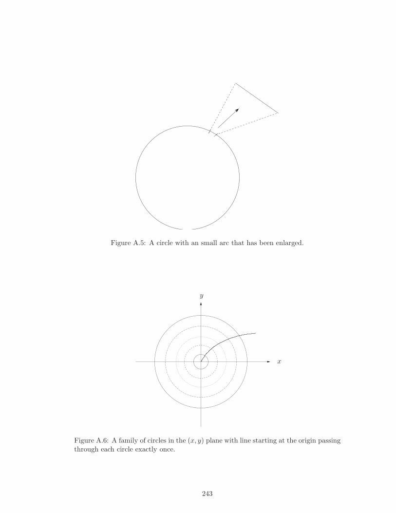
Figure A.5: A circle with an small arc that has been enlarged.
y
x
Figure A.6: A family of circles in the (x, y) plane with line starting at the origin passingthrough each circle exactly once.
243
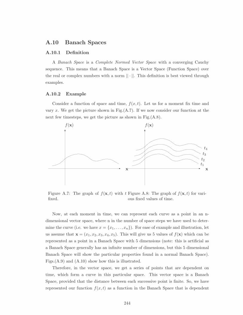
A.10 Banach Spaces
A.10.1 Definition
A Banach Space is a Complete Normed Vector Space with a converging Cauchy
sequence. This means that a Banach Space is a Vector Space (Function Space) over
the real or complex numbers with a norm || · ||. This definition is best viewed through
examples.
A.10.2 Example
Consider a function of space and time, f(x, t). Let us for a moment fix time and
vary x. We get the picture shown in Fig.(A.7). If we now consider our function at the
next few timesteps, we get the picture as shown in Fig.(A.8).
f(x)
x
Figure A.7: The graph of f(x, t) with tfixed.
f(x)
xt1
t2
t3
t4
Figure A.8: The graph of f(x, t) for vari-ous fixed values of time.
Now, at each moment in time, we can represent each curve as a point in an n-
dimensional vector space, where n in the number of space steps we have used to deter-
mine the curve (i.e. we have x = x1, . . . , xn). For ease of example and illustration, let
us assume that x = (x1, x2, x3, x4, x5). This will give us 5 values of f(x) which can be
represented as a point in a Banach Space with 5 dimensions (note: this is artificial as
a Banach Space generally has an infinite number of dimensions, but this 5 dimensional
Banach Space will show the particular properties found in a normal Banach Space).
Figs.(A.9) and (A.10) show how this is illustrated.
Therefore, in the vector space, we get a series of points that are dependent on
time, which form a curve in this particular space. This vector space is a Banach
Space, provided that the distance between each successive point is finite. So, we have
represented our function f(x, t) as a function in the Banach Space that is dependent
244
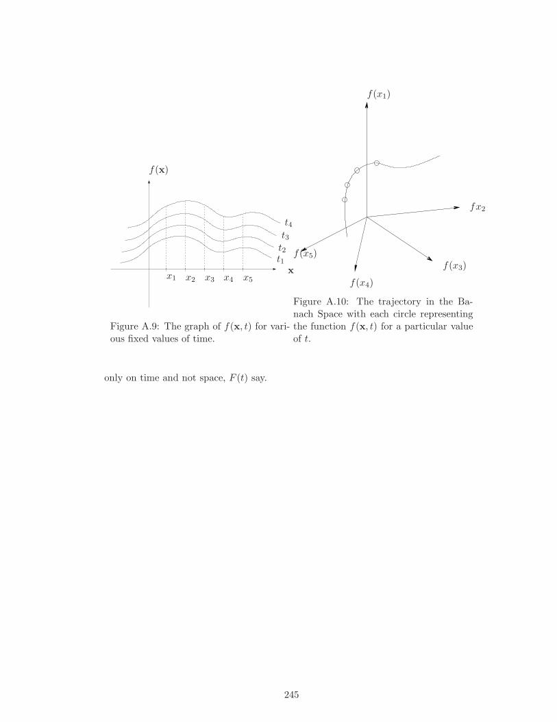
f(x)
xt1
t2
t3
t4
x1 x2 x3 x4 x5
Figure A.9: The graph of f(x, t) for vari-ous fixed values of time.
f(x1)
fx2
f(x3)
f(x4)
f(x5)
Figure A.10: The trajectory in the Ba-nach Space with each circle representingthe function f(x, t) for a particular valueof t.
only on time and not space, F (t) say.
245
Appendix B
EZ-Freeze
EZ-Freeze is a program which simulates spiral waves in a frame of reference which
is moving with the tip of the wave. The motivation behind the program is within [16],
in which the a Reaction-Diffusion-Advection type dynamical system was derived. The
program is based on the very popular program EZ-Spiral by Dwight Barkley [6]. We
refer to [26] for a more complete mathematical analysis of solving spiral waves in the
comoving frame of reference.
EZ-Freeze uses both Barkley’s and FitzHugh-Nagumo’s (FHN) models, together
with a choice of boundary conditions (Neumann or Dirichlet) and whether interactive
graphics are to be used or not.
The following set of intructions are organised as follows:
Section 2 Getting Started: This will talk you through how to get the program
working by following two examples.
Section 3 Users Manual: This will decribe the important uses of EZ-Freeze and
how the user can do particular tasks.
Section 4 Programmers Manual: This section will describe how the program works,
detailing the differences between EZ-Freeze and EZ-Spiral, the function of each
file, and descriptions of the main functions used.
Section 5 Mathematics: We will describe the mathematical problem from which
this program was first conceived, including the numerical methods used within
EZ-Freeze .
B.1 Getting Started: A Quick Guide
We will talk you through getting the program started by following a couple of
examples - one example for a rigidly rotating spiral wave and another example for a
246
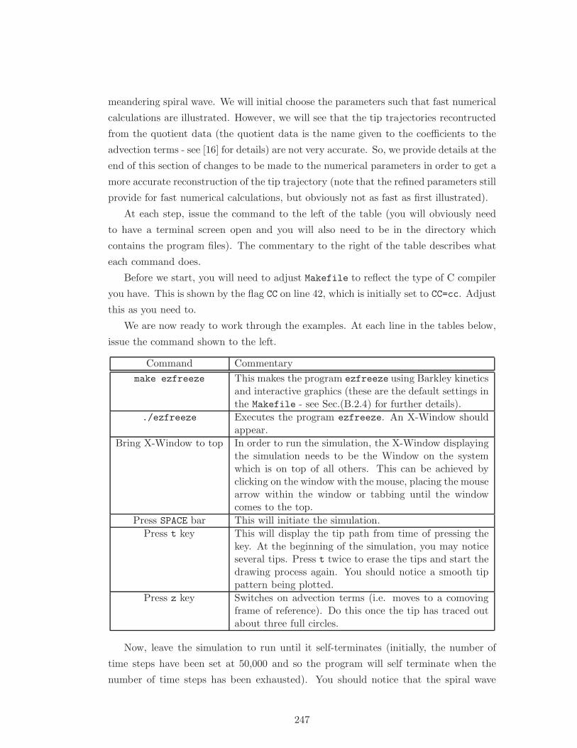
meandering spiral wave. We will initial choose the parameters such that fast numerical
calculations are illustrated. However, we will see that the tip trajectories recontructed
from the quotient data (the quotient data is the name given to the coefficients to the
advection terms - see [16] for details) are not very accurate. So, we provide details at the
end of this section of changes to be made to the numerical parameters in order to get a
more accurate reconstruction of the tip trajectory (note that the refined parameters still
provide for fast numerical calculations, but obviously not as fast as first illustrated).
At each step, issue the command to the left of the table (you will obviously need
to have a terminal screen open and you will also need to be in the directory which
contains the program files). The commentary to the right of the table describes what
each command does.
Before we start, you will need to adjust Makefile to reflect the type of C compiler
you have. This is shown by the flag CC on line 42, which is initially set to CC=cc. Adjust
this as you need to.
We are now ready to work through the examples. At each line in the tables below,
issue the command shown to the left.
Command Commentary
make ezfreeze This makes the program ezfreeze using Barkley kineticsand interactive graphics (these are the default settings inthe Makefile - see Sec.(B.2.4) for further details).
./ezfreeze Executes the program ezfreeze. An X-Window shouldappear.
Bring X-Window to top In order to run the simulation, the X-Window displayingthe simulation needs to be the Window on the systemwhich is on top of all others. This can be achieved byclicking on the window with the mouse, placing the mousearrow within the window or tabbing until the windowcomes to the top.
Press SPACE bar This will initiate the simulation.
Press t key This will display the tip path from time of pressing thekey. At the beginning of the simulation, you may noticeseveral tips. Press t twice to erase the tips and start thedrawing process again. You should notice a smooth tippattern being plotted.
Press z key Switches on advection terms (i.e. moves to a comovingframe of reference). Do this once the tip has traced outabout three full circles.
Now, leave the simulation to run until it self-terminates (initially, the number of
time steps have been set at 50,000 and so the program will self terminate when the
number of time steps has been exhausted). You should notice that the spiral wave
247
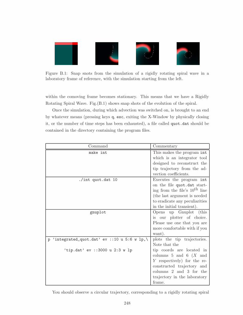
Figure B.1: Snap snots from the simulation of a rigidly rotating spiral wave in alaboratory frame of reference, with the simulation starting from the left.
within the comoving frame becomes stationary. This means that we have a Rigidly
Rotating Spiral Wave. Fig.(B.1) shows snap shots of the evolution of the spiral.
Once the simulation, during which advection was switched on, is brought to an end
by whatever means (pressing keys q, esc, exiting the X-Window by physically closing
it, or the number of time steps has been exhausted), a file called quot.dat should be
contained in the directory containing the program files.
Command Commentary
make int This makes the program int
which is an integrator tooldesigned to reconstruct thetip trajectory from the ad-vection coefficients.
./int quot.dat 10 Executes the program int
on the file quot.dat start-ing from the file’s 10th line(the last argument is neededto eradicate any peculiaritiesin the initial transient).
gnuplot Opens up Gnuplot (thisis our plotter of choice.Please use one that you aremore comfortable with if youwant).
p ’integrated_quot.dat’ ev ::10 u 5:6 w lp,\ plots the tip trajectories.Note that the
’tip.dat’ ev ::3000 u 2:3 w lp tip coords are located incolumns 5 and 6 (X andY respectively) for the re-constructed trajectory andcolumns 2 and 3 for thetrajectory in the laboratoryframe.
You should observe a circular trajectory, corresponding to a rigidly rotating spiral
248
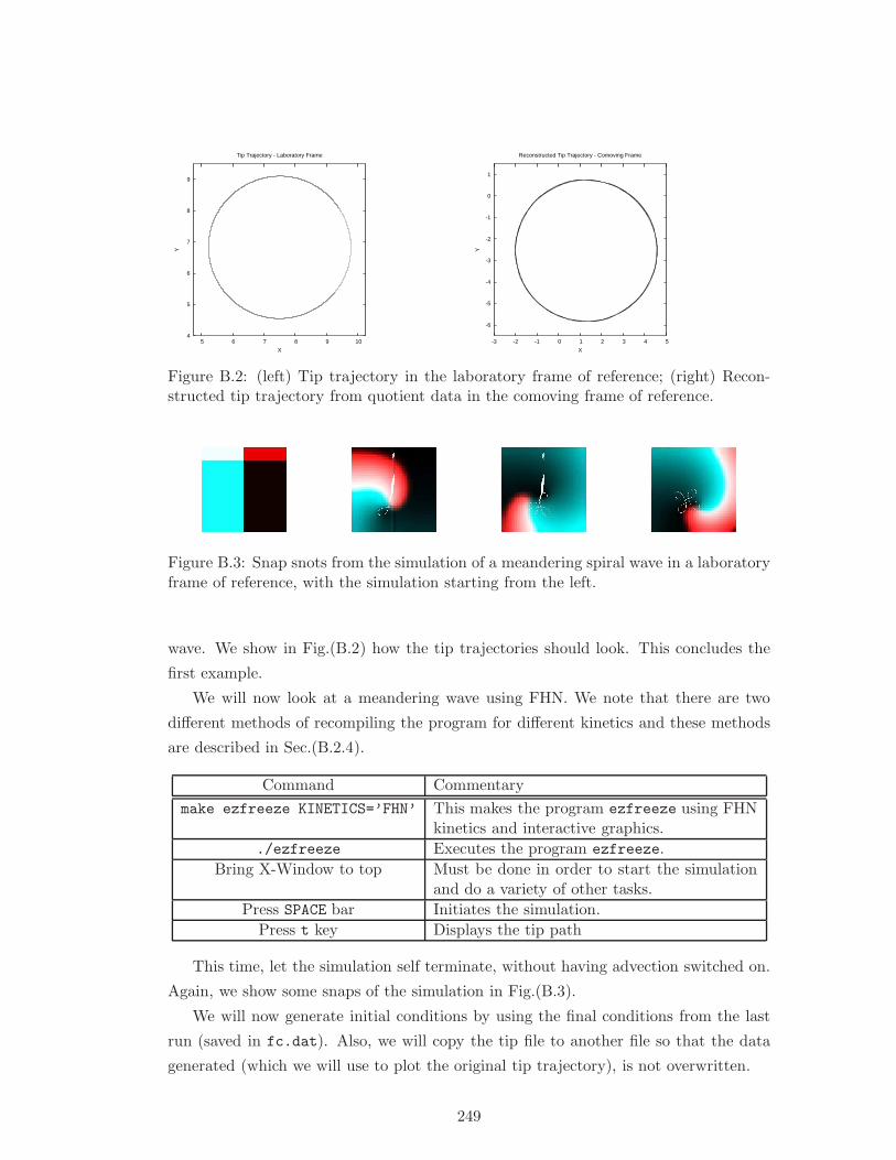
4
5
6
7
8
9
5 6 7 8 9 10
Y
X
Tip Trajectory - Laboratory Frame
-6
-5
-4
-3
-2
-1
0
1
-3 -2 -1 0 1 2 3 4 5
Y
X
Reconstructed Tip Trajectory - Comoving Frame
Figure B.2: (left) Tip trajectory in the laboratory frame of reference; (right) Recon-structed tip trajectory from quotient data in the comoving frame of reference.
Figure B.3: Snap snots from the simulation of a meandering spiral wave in a laboratoryframe of reference, with the simulation starting from the left.
wave. We show in Fig.(B.2) how the tip trajectories should look. This concludes the
first example.
We will now look at a meandering wave using FHN. We note that there are two
different methods of recompiling the program for different kinetics and these methods
are described in Sec.(B.2.4).
Command Commentary
make ezfreeze KINETICS=’FHN’ This makes the program ezfreeze using FHNkinetics and interactive graphics.
./ezfreeze Executes the program ezfreeze.
Bring X-Window to top Must be done in order to start the simulationand do a variety of other tasks.
Press SPACE bar Initiates the simulation.
Press t key Displays the tip path
This time, let the simulation self terminate, without having advection switched on.
Again, we show some snaps of the simulation in Fig.(B.3).
We will now generate initial conditions by using the final conditions from the last
run (saved in fc.dat). Also, we will copy the tip file to another file so that the data
generated (which we will use to plot the original tip trajectory), is not overwritten.
249
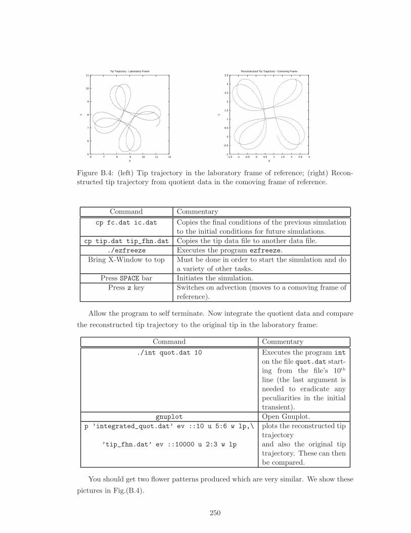
5
6
7
8
9
10
11
6 7 8 9 10 11 12
Y
X
Tip Trajectory - Laboratory Frame
-1
-0.5
0
0.5
1
1.5
2
2.5
3
3.5
-1.5 -1 -0.5 0 0.5 1 1.5 2 2.5 3
Y
X
Reconstructed Tip Trajectory - Comoving Frame
Figure B.4: (left) Tip trajectory in the laboratory frame of reference; (right) Recon-structed tip trajectory from quotient data in the comoving frame of reference.
Command Commentary
cp fc.dat ic.dat Copies the final conditions of the previous simulationto the initial conditions for future simulations.
cp tip.dat tip_fhn.dat Copies the tip data file to another data file.
./ezfreeze Executes the program ezfreeze.
Bring X-Window to top Must be done in order to start the simulation and doa variety of other tasks.
Press SPACE bar Initiates the simulation.
Press z key Switches on advection (moves to a comoving frame ofreference).
Allow the program to self terminate. Now integrate the quotient data and compare
the reconstructed tip trajectory to the original tip in the laboratory frame:
Command Commentary
./int quot.dat 10 Executes the program int
on the file quot.dat start-ing from the file’s 10th
line (the last argument isneeded to eradicate anypeculiarities in the initialtransient).
gnuplot Open Gnuplot.
p ’integrated_quot.dat’ ev ::10 u 5:6 w lp,\ plots the reconstructed tiptrajectory
’tip_fhn.dat’ ev ::10000 u 2:3 w lp and also the original tiptrajectory. These can thenbe compared.
You should get two flower patterns produced which are very similar. We show these
pictures in Fig.(B.4).
250
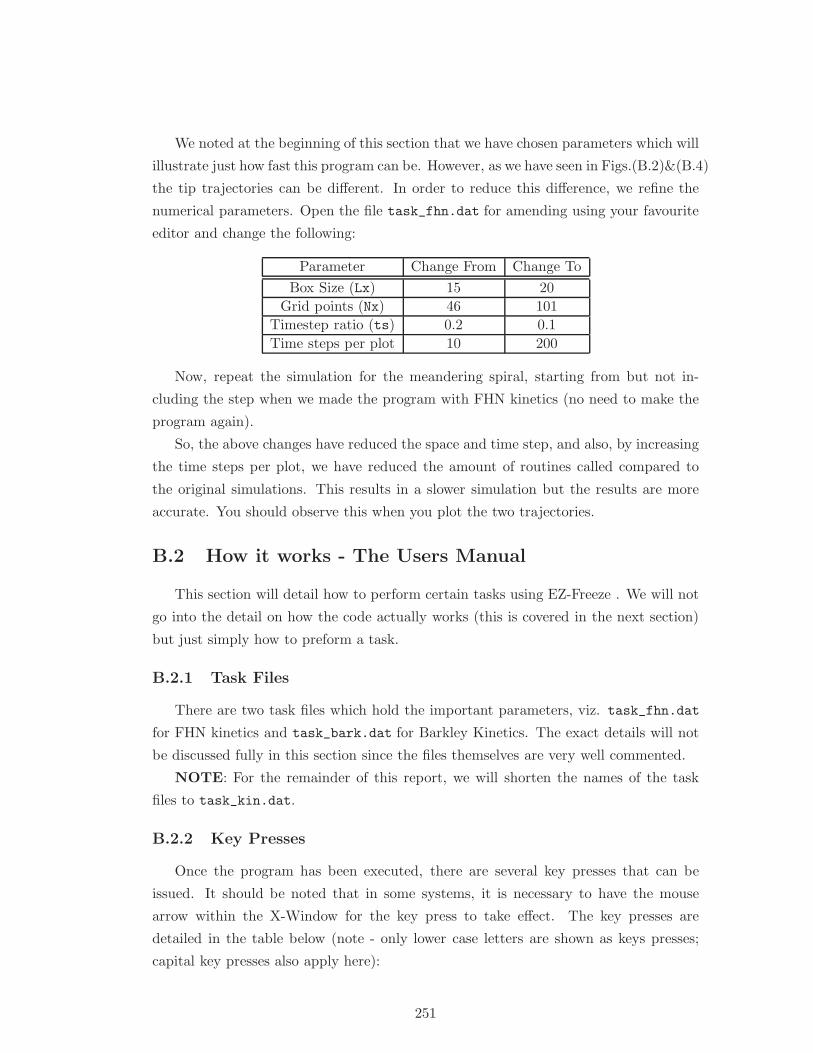
We noted at the beginning of this section that we have chosen parameters which will
illustrate just how fast this program can be. However, as we have seen in Figs.(B.2)&(B.4)
the tip trajectories can be different. In order to reduce this difference, we refine the
numerical parameters. Open the file task_fhn.dat for amending using your favourite
editor and change the following:
Parameter Change From Change To
Box Size (Lx) 15 20
Grid points (Nx) 46 101
Timestep ratio (ts) 0.2 0.1
Time steps per plot 10 200
Now, repeat the simulation for the meandering spiral, starting from but not in-
cluding the step when we made the program with FHN kinetics (no need to make the
program again).
So, the above changes have reduced the space and time step, and also, by increasing
the time steps per plot, we have reduced the amount of routines called compared to
the original simulations. This results in a slower simulation but the results are more
accurate. You should observe this when you plot the two trajectories.
B.2 How it works - The Users Manual
This section will detail how to perform certain tasks using EZ-Freeze . We will not
go into the detail on how the code actually works (this is covered in the next section)
but just simply how to preform a task.
B.2.1 Task Files
There are two task files which hold the important parameters, viz. task_fhn.dat
for FHN kinetics and task_bark.dat for Barkley Kinetics. The exact details will not
be discussed fully in this section since the files themselves are very well commented.
NOTE: For the remainder of this report, we will shorten the names of the task
files to task_kin.dat.
B.2.2 Key Presses
Once the program has been executed, there are several key presses that can be
issued. It should be noted that in some systems, it is necessary to have the mouse
arrow within the X-Window for the key press to take effect. The key presses are
detailed in the table below (note - only lower case letters are shown as keys presses;
capital key presses also apply here):
251
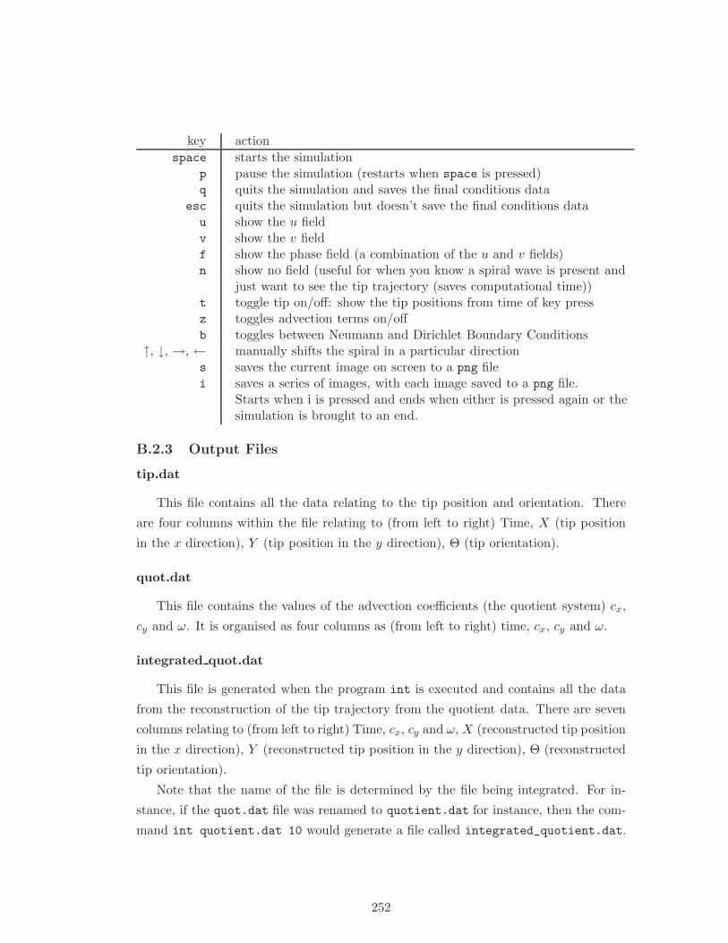
key action
space starts the simulationp pause the simulation (restarts when space is pressed)q quits the simulation and saves the final conditions data
esc quits the simulation but doesn’t save the final conditions datau show the u fieldv show the v fieldf show the phase field (a combination of the u and v fields)n show no field (useful for when you know a spiral wave is present and
just want to see the tip trajectory (saves computational time))t toggle tip on/off: show the tip positions from time of key pressz toggles advection terms on/offb toggles between Neumann and Dirichlet Boundary Conditions
↑, ↓, →, ← manually shifts the spiral in a particular directions saves the current image on screen to a png filei saves a series of images, with each image saved to a png file.
Starts when i is pressed and ends when either is pressed again or thesimulation is brought to an end.
B.2.3 Output Files
tip.dat
This file contains all the data relating to the tip position and orientation. There
are four columns within the file relating to (from left to right) Time, X (tip position
in the x direction), Y (tip position in the y direction), Θ (tip orientation).
quot.dat
This file contains the values of the advection coefficients (the quotient system) cx,
cy and ω. It is organised as four columns as (from left to right) time, cx, cy and ω.
integrated quot.dat
This file is generated when the program int is executed and contains all the data
from the reconstruction of the tip trajectory from the quotient data. There are seven
columns relating to (from left to right) Time, cx, cy and ω, X (reconstructed tip position
in the x direction), Y (reconstructed tip position in the y direction), Θ (reconstructed
tip orientation).
Note that the name of the file is determined by the file being integrated. For in-
stance, if the quot.dat file was renamed to quotient.dat for instance, then the com-
mand int quotient.dat 10 would generate a file called integrated_quotient.dat.
252
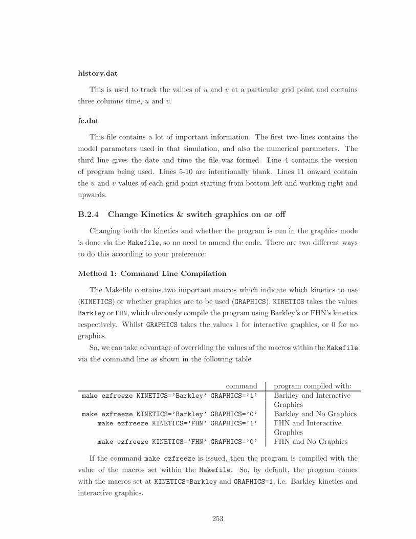
history.dat
This is used to track the values of u and v at a particular grid point and contains
three columns time, u and v.
fc.dat
This file contains a lot of important information. The first two lines contains the
model parameters used in that simulation, and also the numerical parameters. The
third line gives the date and time the file was formed. Line 4 contains the version
of program being used. Lines 5-10 are intentionally blank. Lines 11 onward contain
the u and v values of each grid point starting from bottom left and working right and
upwards.
B.2.4 Change Kinetics & switch graphics on or off
Changing both the kinetics and whether the program is run in the graphics mode
is done via the Makefile, so no need to amend the code. There are two different ways
to do this according to your preference:
Method 1: Command Line Compilation
The Makefile contains two important macros which indicate which kinetics to use
(KINETICS) or whether graphics are to be used (GRAPHICS). KINETICS takes the values
Barkley or FHN, which obviously compile the program using Barkley’s or FHN’s kinetics
respectively. Whilst GRAPHICS takes the values 1 for interactive graphics, or 0 for no
graphics.
So, we can take advantage of overriding the values of the macros within the Makefile
via the command line as shown in the following table
command program compiled with:
make ezfreeze KINETICS=’Barkley’ GRAPHICS=’1’ Barkley and InteractiveGraphics
make ezfreeze KINETICS=’Barkley’ GRAPHICS=’0’ Barkley and No Graphicsmake ezfreeze KINETICS=’FHN’ GRAPHICS=’1’ FHN and Interactive
Graphicsmake ezfreeze KINETICS=’FHN’ GRAPHICS=’0’ FHN and No Graphics
If the command make ezfreeze is issued, then the program is compiled with the
value of the macros set within the Makefile. So, by default, the program comes
with the macros set at KINETICS=Barkley and GRAPHICS=1, i.e. Barkley kinetics and
interactive graphics.
253
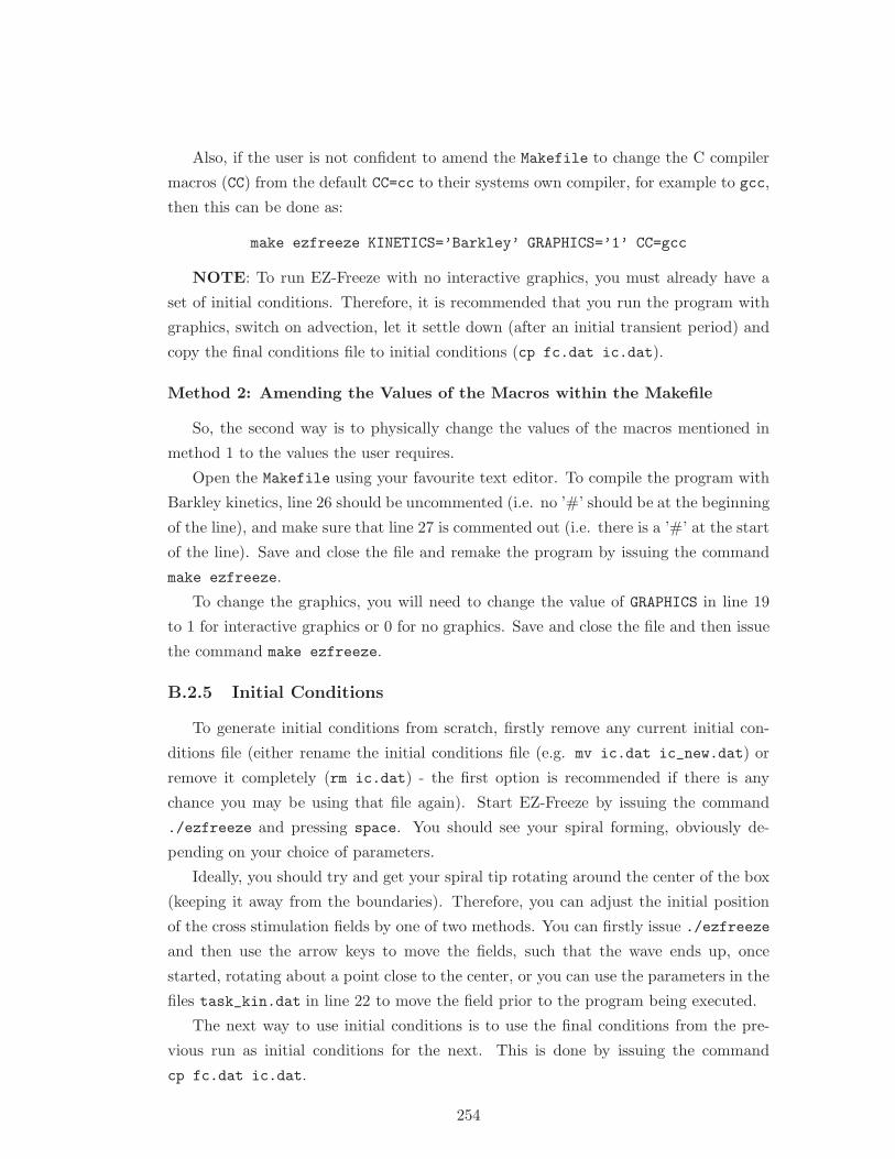
Also, if the user is not confident to amend the Makefile to change the C compiler
macros (CC) from the default CC=cc to their systems own compiler, for example to gcc,
then this can be done as:
make ezfreeze KINETICS=’Barkley’ GRAPHICS=’1’ CC=gcc
NOTE: To run EZ-Freeze with no interactive graphics, you must already have a
set of initial conditions. Therefore, it is recommended that you run the program with
graphics, switch on advection, let it settle down (after an initial transient period) and
copy the final conditions file to initial conditions (cp fc.dat ic.dat).
Method 2: Amending the Values of the Macros within the Makefile
So, the second way is to physically change the values of the macros mentioned in
method 1 to the values the user requires.
Open the Makefile using your favourite text editor. To compile the program with
Barkley kinetics, line 26 should be uncommented (i.e. no ’#’ should be at the beginning
of the line), and make sure that line 27 is commented out (i.e. there is a ’#’ at the start
of the line). Save and close the file and remake the program by issuing the command
make ezfreeze.
To change the graphics, you will need to change the value of GRAPHICS in line 19
to 1 for interactive graphics or 0 for no graphics. Save and close the file and then issue
the command make ezfreeze.
B.2.5 Initial Conditions
To generate initial conditions from scratch, firstly remove any current initial con-
ditions file (either rename the initial conditions file (e.g. mv ic.dat ic_new.dat) or
remove it completely (rm ic.dat) - the first option is recommended if there is any
chance you may be using that file again). Start EZ-Freeze by issuing the command
./ezfreeze and pressing space. You should see your spiral forming, obviously de-
pending on your choice of parameters.
Ideally, you should try and get your spiral tip rotating around the center of the box
(keeping it away from the boundaries). Therefore, you can adjust the initial position
of the cross stimulation fields by one of two methods. You can firstly issue ./ezfreeze
and then use the arrow keys to move the fields, such that the wave ends up, once
started, rotating about a point close to the center, or you can use the parameters in the
files task_kin.dat in line 22 to move the field prior to the program being executed.
The next way to use initial conditions is to use the final conditions from the pre-
vious run as initial conditions for the next. This is done by issuing the command
cp fc.dat ic.dat.
254
B.2.6 Change Box Size
The box size is amended in task_kin.dat. The parameters are called Lx and Ly
and are located on line 4. Also, to perserve a particular spacestep, you will need to
change Nx and Ny accordingly.
B.2.7 Change Timestep
The timestep can be changed by amending ts in the task_kin.dat file on line 8.
B.2.8 History File
If you feel that you need to observe a particular feature of the spiral wave by
observing how u and v change over time, then you can activate the history file. This is
done within task.dat.
Open up task_kin.dat. On line 15, you can specify how many time steps per write
to the history file (called history.dat). If this is zero then no history file is written.
Also, you can change the point which is being used as the history point on line 16.
B.2.9 Changing Boundary Conditions
This is done via pressing b. The default BC’s are set via the task_kin.dat file on
line 23.
B.2.10 Change Position of Second Pinning Point
Within task_kin.dat (on line 17) there are of parameters called x_inc and y_inc.
Adjusting the values of these will change the position of the second pinning point.
WARNING: Setting x_inc and y_inc to zero simultaneously will give a division
by zero if advection is switched on (i.e. by pressing z). When the program is executed,
a warning is displaying on the terminal screen if they are zero. The program will still
run in the stationary frame (Laboratory Frame) of reference, but will terminate once
advection is switched on.
B.2.11 Change Orientation of Tip in the Comoving Frame of Refer-ence
This follows on from the preceding subsection (Change Position of Second Pinning
Point). By changing the second pinning point, you will actually change the fixed
orientation of the tip in the comoving frame of reference. Note the warning in the
above section.
255
B.3 How it works - The Programmers Manual
This section will describe how particular parts of the code work. We firstly detail
the main differences between EZ-Freeze and EZ-Spiral
B.3.1 Differences between EZ-Freeze and EZ-Spiral
1. Kinetics - FHN kinetics have been incorporated into EZ-Freeze via ezstep.h.
Also, different parameters are needed for FHN compared to Barkley kinetics and
therefore this is incorporated throughout the code.
2. Boundary Conditions - Dirichlet BC’s have been incorporated. Switching between
Neumann and Dirichlet BC’s is done by pressing b.
3. Advection Calculation - Advection terms are calculated via the function step1()
found in ezstep.c.
4. Phase Field - this is a combination of the u and v-fields, switched on by pressing
f.
5. Output - tip.dat now holds the orientation of the tip as well as its spatial
coordinates; quot.dat, created when advection is calculated, holds the values of
the coefficients of the advection terms, i.e. cx, cy and ω.
6. Saving Images - the user can now save just a single image to a png file (pressing
s) or a series of images to a series of png files (pressing i).
7. Task Files - there are now two task files (one for Barkley kinetics, one for FHN).
The program will choose which is necessary upon compilation.
8. Makefile - there are now options via the Makefile to make the program with a
particular set of kinetics and whether interactive graphics are used.
256
B.3.2 Files
File Description
ezfreeze.c Contains the main function files,including reading in parametersfrom task files, allocation ofmemory, initialising the simula-tion.
ezfreeze.h Contains all the global variablesneeded in the code and some ofthe major macros.
ezstep.c Contains procedures to calcu-late the values of the variablesu(x, y, t) and v(x, y, t) for eachtime step, as well as the bound-ary conditions
ezstep.h Contains mainly the algorithmsfor the kinetics.
ezgraphGL.c Contains the code for graphicalsimulations.
ezgraphGL.h Contains the macros for thegraphical simulations.
eztip.c Contains the procedures to findthe tip position and orientation.
Makefile Makes the program, as well asclean up the files and compressthem if the user wishes.
task_fhn.dat, task_bark.dat Task files containing the physi-cal and numerical parameters, aswell as some important flags.
It is intended that the user will not only use the program as it is, but will amend
it to suit their needs. We therefore detail in the following subsections, the important
functions that are used in EZ-Freeze , including where they are found and what they
do.
Makefile
The Makefile contains several commands to compile ezfreeze (the main simulat-
ing program) and int (which can be used to integrate the quotient data). We refer
the reader to Sec.(B.2.4) for information on how to compile the program for particular
kinetics and choice of graphics.
It is assumed that the user is fluent in UNIX commands and can therefore am
mend any of the files in this package to suit their needs - in particular the command in
Makefile which refers to their systems particular C compiler. However, if the user is
257
not fluent in UNIX commands the user can still compile the program via the command
line without having to go into the Makefile (see Sec.(B.2.4)).
The main method which is implemented in the Makefile is the way in which the
program ezfreeze is compiled. The two major macros integrated within Makefile
are KINETICS and GRAPHICS, which determine which Kinetics are used and whether to
use graphics respectively. The values of these macros are passed to the compilation
command line via the macro CFLAGS using the preprocessor command -DFHN=$(KIN)
and -DGRAPHICS=$(GRAPH), where KIN is either 1 (for FHN kinetics) or 0 (for Barkley),
and GRAPH is either 1 (for graphics) or 0 (for no graphics).
It is assumed that the user is fluent in UNIX commands and can therefore amend
any of the files in this package to suit their needs - in particular the command in
Makefile which refers to their systems particular C compiler.
Also in Makefile are several cleaning up processes such as make tidy (deletes the
object files and executable ezfreeze) and make clean (does what make tidy does,
plus deletes several other files including any files created when the manual is formed
and *.*∼ files).
ezfreeze.c
This file contains a number of important functions. The most important function is
main. Within the main function the whole program is initialised (via Initialise()),
and then the main loop is executed. Within the loop there are calls of the step functions
which calculate the values of u(x, y, t) and v(x, y, t) (see Sec.(B.3.2)), and then the
drawing routines are called.
Also in the main function there is a timer which calculates the time the whole
simulation has taken (in real time). This will prove useful when comparing the time
taken for particular simulations.
Also, in ezfreeze.c, there are various other functions. Two of these functions,
cube() and root(), calculate the steady state in FHN, which are then used in the
drawing procedure.
Another function is Write_quot(float cx, float cy, float om), which writes
the quotient data (cx, cy and ω) to a file called quot.dat. However, this function is
only called when all three components are being calculated (see Sec.(B.3.2) for more
details).
Finally, the way that initial conditions are generated via Generate_ic() has been
amended slightly so that the position of the cross field stimulations can be controlled
via the variables found in task_kin.dat on line 22.
258
ezfreeze.h
This file is the main header file, used in all the other files, and contains mainly
macros used throughout the program and also declares the global variables.
ezstep.c
There are three main functions contained in this file.
The first is step(). This was originally contained in ezstep.c used in EZ-Spiral,
and it’s purpose is to calculate the values of u(x, y, t) and v(x, y, t) for each time step
for the Reaction-Diffusion part of the equation. Operator splitting can be used here
(switched on via the macro SPLIT found in ezfreeze.h).
The next function is step1(), which calculates the final values of u(x, y, t) and
v(x, y, t) when advection is switched on. For a more detailed analysis, please see
Sec.(B.4.2).
Finally, we have amended the function Impose_boundary_conditions() to include
Dirichlet boundary conditions as well as Neumann boundary conditions.
ezstep.h
This relatively short file contains all the macros for the kinetics used in step() and
step1().
eztip.c
This file is entirely devoted to finding the tip position. It has only been amended
slightly from the eztip.c used for EZ-Spiral. The main changes are firstly the calcu-
lation of the orientation of the tip, and also the variable MAX_TIPS has been increased
to 10,000,000 to allow for long simulations (this can be increased if needed).
ezgraphGL.c
There have been several changes to this particular file compared to the file used in
EZ-Spiral. The main changes are to the extra key presses. These include key presses to
change the boundary conditions (key b), toggling the switching on/off of the advection
terms (key z), toggling between the way the advection coefficients (quotient system) is
calculated (key e), save images (keys s and i), and change to a phase field (combination
of u and v-fields; key press f).
Associates with these keys presses are functions which execute the action that the
key press is for.
259
ezgraphGL.h
Nothing has been amended in this file from that used in EZ-Spiral. This file contains
a variety of macros used in the drawing routines of the spiral wave.
B.4 Mathematical Background
The original idea behind EZ-Freeze was twofold. Firstly, we intended EZ-Freeze to
be used as a tool for which computational time can be significantly reduced. Secondly,
for the first time, it can be used as a tool in order to study the limit cycles behind
the dynamics of meandering spiral waves. There are other uses of EZ-Freeze such as
calculation of the critical eigenvalues of the spiral, which are discussed in [26].
With regards to the first use, computational time is reduced significantly because
the tip of the wave is always located at the center of the computational box. This
means that the tip of the wave never reaches the boundary of the box. Therefore a
smaller box size can be afforded. One of the applications of this technique, as detailed
in [26] is to study 1:1 resonance in meandering spiral waves. In [26], we show a study
in which the box size is Lx = Ly = 15s.u. in the comoving frame with Nx = Ny = 76
grid points in each direction. But in the laboratory frame of reference, the trajectory
should have been Lx = Ly = 700s.u. with Nx = Ny = 3500 grid points in each
direction. Therefore, we see that the simulation in the comoving frame reduces the
computational time significantly.
B.4.1 Mathematics behind EZ-Freeze
The system of equations that we are solving is a 2 species Reaction-Diffusion-
Advection system as shown below:
∂u
∂t= ∇2u + f(u, v) + (c,∇)u + ω
∂u
∂θ(B.1)
∂v
∂t= δ∇2v + g(u, v) + (c,∇)v + ω
∂v
∂θ(B.2)
where f(u, v) and g(u, v) are the reaction terms (kinetics) of the systems. EZ-Freeze
implements two different types of kinetics - Barkley’s and FHN’s.
Barkley: f(u, v) = 1ǫu(1− u)(u− v+b
a) , g(u, v) = (u− v)
FHN: f(u, v) = 1ǫ(u− u3
3 − v) , g(u, v) = ǫ(u + β − γv)
In both systems, δ is the ratio of diffusion coefficients (typically taken as δ=0 or
δ=1), and the model parameters are β, γ and ǫ for FHN, and a, b and ǫ for Barkley.
260
In both cases, ǫ determines the slow and fast times of the systems. We further refer to
[10] and [63] which show parametric portraits for each model fixing one parameter and
varying the others. The user of EZ-Freeze is urged to use these parametric portraits
when trying out EZ-Freeze to determine the parameters for a particular type of spiral
wave.
In order to “pin” the tip to a particular position and with a particular orientation,
we need three conditions (the three are for fixing the position in x and y directions and
also the phase angle). We decided that due to the sensitivity of calculating the ω, we
would use two different sets of conditions:
Tip Pinning Tip PinningConditions 1 Conditions 2
u(xtip, ytip) = u∗ u(xtip, ytip) = u∗
v(xtip, ytip) = v∗ v(xtip, ytip) = v∗∂u∂x
(xtip, ytip) = 0 u(xtip + xinc, ytip + yinc) = u∗
where (xtip, ytip) are the coordinates at the desired tip position and xinc and yinc are
increments away from desired tip position. We note that in Conditions 2, when xinc = 1
and yinc = 0, then we get Conditions 1. We also impose that xinc 6= 0 and yinc 6= 0 in
Conditions 2 otherwise we will get division by zero when calculating ω.
Also, in EZ-Freeze we implement these conditions such that the desired tip position
is at the center of the medium.
B.4.2 Numerical Methods
Firstly, the calculation of the time derivatives are done using an explicit forward
Euler method. Then, the spatial derivatives are done in two parts - the diffusion terms
(solved using either a five or nine point Laplacian method - which to use is chosen by
amending the macro NINEPOINT (0 for five point and 1 for nine point) in ezfreeze.h),
and the advection terms which are calculated using a second order accurate upwind
scheme as shown below:
∂u
∂x
∣
∣
∣
∣
(x,y)
≈ 1
2∆x(−3u(x, y) + 4u(x + ∆x, y)− u(x + 2∆x, y)) (B.3)
or∂u
∂x
∣
∣
∣
∣
(x,y)
≈ 1
2∆x(3u(x, y) − 4u(x−∆x, y) + u(x− 2∆x, y)) (B.4)
where we determine which scheme is used by looking at the sign of the coefficient in
front of the derivative, i.e. if the coefficient is positive, we use scheme (B.3) and vice
261
versa. A first order accurate scheme is not used as we found it did not give accurate
results. A discussion of this can be found in [26].
Throughout the code, we use operator splitting, and in particular we will use the
following scheme:
un+ 1
2i,j = un
i,j + ∆tRD(uni,j, v
ni,j) (B.5)
un+1i,j = u
n+ 12
i,j + ∆tAD(un+ 1
2i,j , v
n+ 12
i,j ) (B.6)
where uni,j is u at the n-th time step and at the grid coordinate (i, j), and RD and
AD are the Reaction-Diffusion and Advection terms respectively, and ∆t is the time
step. Therefore, we note that Eqn.(B.5) is implemented into the program in function
step(), and Eqn.(B.6) via the function step1(). Similar equations also exist for v.
By using operator splitting in this way, we can formulate a system of three linear
equations in cx, cy, and ω which can easily be solved. It turns out that, after using the
tip pinning conditions, we get the following linear system:
cx∂u
∂x+ cy
∂u
∂y=
∂u
∂t(B.7)
cx∂v
∂x+ cy
∂v
∂y=
∂v
∂t(B.8)
cx∂u
∂x+ cy
∂u
∂y+ ω
(
x∂u
∂y− y
∂u
∂x
)
=∂u
∂t(B.9)
where
u = unNX2
, NY2
(B.10)
v = vnNX2
, NY2
(B.11)
u = unNX2
+x inc, NY2
+y incx inc, y inc > 1 (B.12)
These are the main numerical procedures implemented into EZ-Freeze.
Finally, the integrator program int solves the following equations:
dR
dt= ceiΘt (B.13)
dΘ
dt= ω (B.14)
where R = X + iY is the tip position, and Θ is it’s orientation. c = cx + icy is the
translational velocity of the tip and ω is its angular velocity.
262
Eqns.(B.13) and (B.14) are numerically integrated using the following scheme:
Θn+1 = Θn + ∆tωn (B.15)
Xn+1 = Xn + ∆t(cnx cos(Θ)− cn
y sin(Θ)) (B.16)
Y n+1 = Y n + ∆t(cnx sin(Θ) + cn
y cos(Θ)) (B.17)
where the superscript represents what time step we are at and ∆t is the value of the
time step increment.
263
Bibliography
[1] K. Agladze, J.P. Keener, S.C. Muller, and A.V. Panfilov. “Rotating Spiral Waves
Created by Geometry”. Science, 264:1746 – 1748, 1994.
[2] K.I. Agladze, V.A. Davydov, and A.S. Mikhailov. “Observation of a Spiral Wave
Resonance in an Excitable Disturbed Medium”. JETP Letters, 45(12):767–770,
1987.
[3] E. Anderson, Z. Bai, C. Bischof, S. Blackford, J. Demmel, J. Dongarra, J. Du Croz,
A. Greenbaum, S. Hammarling, A. McKenney, and D. Sorensen. “LAPACK, ver-
sion 3.1.1”, http://www.netlib.org/lapack/, February 2007.
[4] D.V. Anosov and V.I. Arnold. “Dynamical Systems I”. Springer-Verlag, 1985.
[5] V.I. Arnold. “Small Denominators. I Mappings of the Circumference onto Itself”.
Translations of the AMS 2nd Series, 46:213–284, 1965.
[6] D. Barkley. “http://www.maths.warwick.ac.uk/˜barkley”.
[7] D. Barkley. “http://www.scholarpedia.org/article/barkley model”.
[8] D. Barkley. “A Model for Fast Computer Simulation of Waves in Excitable Media”.
Physica D, 49:61 – 70, 1991.
[9] D. Barkley. “Euclidean Symmetry and the Dynamics of Rotating Spiral Waves”.
Physical Review Letters, 72(1), 1994.
[10] D. Barkley and I. Kevrekidis. “A Dymanical Systems Approach to Spiral Wave
Dynamics”. Chaos, pages 453 – 460, 1994.
[11] D. Barkley, M. Kness, and L. S. Tuckerman. “Spiral Wave Dynamics in a Simple
Model of Excitable Media: The Transition from Simple to Compound Rotation”.
Physical Review A, 42(4):2489, 1990.
[12] B. P. Belousov. “A Periodic Reaction and its Mechanism”. Collection of Short
Papers on Radiation Medicine, 10:145 – 152, 1959.
264
[13] W.J. Beyn and V.. Thummler. “Freezing Solutions of Equivariant Evolution Equa-
tions”. SIAM J. Appl. Dyn. Syst., 3(2):85–116, 2004.
[14] V.N. Biktashev and A.V. Holden. “Resonant Drift of Autowave Vortices in 2D
and the Effects of Boundaries and Inhomogeneities”. Chaos, Solitons and Fractals,
5(3,4):575, 1995.
[15] V.N. Biktashev, A.V. Holden, and Yu.E. Elkin. On the Movement of Excitation
Wave Breaks. Chaos, Solitons an Fractals, 9(9):1597 – 1610, 1998.
[16] V.N. Biktashev, A.V. Holden, and E.V. Nikolaev. Spiral Wave Meander and Sym-
metry of the Plane. International Journal of Bifurcation and Chaos, 6(12A):2433,
1996.
[17] V.N. Biktashev, A.V. Holden, and E.V. Nikolaev. On Feedback Resonant Drift and
Interaction with the Boundary in Circular and Annular Excitable Media. Chaos,
Solitons an Fractals, 9(3)0:363 – 376, 1998.
[18] V.N. Biktashev, A.V. Holden, and H Zhang. “Tension of Organizing Filaments of
Scroll Waves”. Phi. Trans. R. Soc Lond. A, 347:611–630, 1994.
[19] I.V. Biktasheva, D. Barkley, V.N. Biktashev, A.J. Foulkes, and G.V. Bordyugov.
Computation of the Response Functions of Spiral Wave in Active Media. In
Preparation, 2008.
[20] I.V. Biktasheva and V.N. Biktashev. Wave-Particle Dualism of Spiral Wave Dy-
namics. Physical Review E, 67, 2003.
[21] L.B. Bushard. “Periodic Solutions and Locking-In on the Periodic Surface”. In-
ternational Journal of Non-Linear Mechanics, 8:129 – 141, 1973.
[22] P Chossat. “The Reduction of Equivariant Dynamics to the Orbit Space for Com-
pact Group Actions”. Acta Applicandae Mathematicae, 70:71–94, 2002.
[23] V.A. Davydov, V.S. Zykov, A.S. Mikhailov, and P.K. Brazhnik. “Drift and Reso-
nance of Spiral Waves in Disturbed Media”. Izv. Vuzov - Radiofizika, 31(5):574,
1988.
[24] R. Fitzhugh. “Impulses and Physiological States in Theoretical Models of Nerve
Membrane”. Biophys. J., 445, 1961.
[25] G. Floquet. “Sur les Equations Differentielles Lineaires a Coefficients Periodiques”.
Annales Scientifiques de L’Ecole Normale Superieure Ser. 2,, 12:47–88, 1883.
265
[26] A.J. Foulkes and V.N. Biktashev. “Spiral Wave Solutions in a Comoving Frame
of Reference: Numerical Implementation and Applications”. In preparation, 2009.
[27] Y.P. Golovachov. “Nnumerical Simulation of Viscous Shock Layer Flows”.
Springer, 1995.
[28] M. Golubitsky, V.G. LeBlanc, and I. Melbourne. “Meandering of the Spiral Tip:
An Alternative Approach”. Journal of Nonlinear Science, 7:557–586, 1997.
[29] V. Hakim and A. Karma. “Spiral Wave Meander in Excitable Media: The Large
Core Limit”. Physical Review Letters, 79(4), 1997.
[30] V Hakim and A. Karma. “Theory of Spiral Wave Dynamics in Weakly Excitable
Media: Asymptotic Reduction to a Kinematic Model and Applications”. Physical
Review E, 60(5), 1999.
[31] R.H. Hall. “Resonance Zones in Two-Parameter Families of Circle Homeomor-
phisms”. SIAM Journal of Mathematical Analysis, 15(6):1075–1081, 1999.
[32] R.B. Hoyle. “Pattern Formation: An Introduction to Methods”. Oxford University
Press, 2006.
[33] J.F. Humphreys. “A Course in Group Theory”. Oxford Science Publications,
1996.
[34] I. Idris. “Initiation of Excitation Waves”. Ph.D Thesis, 2008.
[35] D.W. Jordon and P. Smith. “Nonlinear Ordinary Differential Equations: An In-
troduction to Dynamical Systems”. Oxford University Press, 1999.
[36] A Karma. “Meandering Transition in 2-Dimensional Excitable Media”. Physical
Review Letters, 65(22):2824, 1990.
[37] J. Keener and J. Sneyd. “Mathematical Physiology”. Springer, 2004.
[38] J.P. Keener. “The Dynamics of Three-Dimensional Scroll Waves in Excitable
Media”. Physica D, 31:269, 1988.
[39] V.I. Krinsky. “Fibrillation in the Excitable Media”. Problemy Kibernetiki, 2(1):59,
1968.
[40] V.I. Krinsky and K.I. Agladze. “Interaction of Rotating Waves in an Active Chem-
ical Medium”. Physica D, 8(1-2):50, 1983.
266
[41] S. Kumar. “Krylov Subspace Methods for the Eigenvalue problem”, http://www-
cse.ucsd.edu/classes/fa04/cse252c/sakumar.pfd.
[42] Y.A. Kuznetsov. “Elements of Applied Bifurcation Theory”. Springer-Verlag, 1995.
[43] V.G. LeBlanc. “Rotational Symmetry-Breaking for Spiral Waves”. Nonlinearity,
15:1179 – 1203, 2002.
[44] V.G. LeBlanc and C. Wulff. “Translational Symmetry-Breaking for Spiral Waves”.
Journal of Nonlinear Science, 10:569 – 601, 2000.
[45] W. Ledermann and A. Wier. “Introduction to Group Theory”. Longman, 1996.
[46] R.B. Lehoucq, D.C. Sorensen, and C. Yang. “ARPACK Users Guide: Solution of
Large Scale Eigenvalue Problems by Implicitly Restarted Arnoldi Methods”, 1997.
[47] E. Lugosi. “Analysis of Meandering in Zykov Kinetics”. Physica D, 40:331 – 337,
1989.
[48] J.D. Murray. “Mathematical Biology”. Springer: Interdisciplinary Applied Math-
ematics, Vols 17 & 18, 2003.
[49] J. Nagumo, S. Arimoto, and S. Yoshizawa. “An Active Pulse Transmission Simu-
lating Nerve Axon”. Proc. IRE, 50:2061, 1962.
[50] A. Nayfeh. “Perturbation Methods”. John Wiley & Sons, 1973.
[51] A. Panfilov and A.M. Pertsov. “Mechanism of Spiral Waves Initiation in Active
Media Connected with Critical Curvature Phenomenon.”. Biofizika, 27:886 – 888,
1982.
[52] A.V. Panfilov and A.N. Rudenko. “Two Regimes of the Scroll Ring Drift in the
Three-Dimensional Active Media”. Physica D, 28:215–218, 1987.
[53] A.M. Pertsov and E.A. Ermakova. “Mechanism of the Drift of a Spiral Wave in
an Inhomogeneous Medium.”. Biofizika, 33(2):338–342, 1988.
[54] B Sandstede and A Scheel. “Spiral Superstructures in Meandering and Drifting
Spiral Waves”. Physical Review Letters, 86(1):172–174, 2001.
[55] G. S. Skinner and H. L. Swinney. “Periodic to Quasiperiodic Transition of Chem-
ical Spiral Rotation”. Physica D, 48:1 – 16, 1991.
[56] A.M. Turing. “The Chemical Basis of Morphogenesis”. Phil. Trans. Roy. Soc.
Lond., 237:37 – 72, 1952.
267
[57] J.J. Tyson and J.P. Keener. “Singular Perturbation Theory of Traveling Waves
in Excitable Media”. Physica D, 32:327, 1988.
[58] P. Wheeler and D. Barkley. “Computation of Spiral Spectra”. SIAM Journal of
Applied Dynamical Systems, 5(1):157 – 177, 2006.
[59] N. Wiener and A. Rosenbleuth. “The Mathematical Formulation of the Prob-
lem of Conduction in Impulses in a Network of Conducted Excitable Elements,
Specifically in Cardiac Muscle”. Arch. Inst. Cardiol. Mex., 16:205 – 265, 1946.
[60] S. Wiggins. “Introduction to Applied Nonlinear Dynamical Systems and Chaos”.
Springer, 2003.
[61] A.T. Winfree. “Spiral Waves of Chemical Activity”. Science, 175:634 – 636, 1972.
[62] A.T. Winfree. “When Time Breaks Down”. Princeton University Press, 1987.
[63] A.T. Winfree. “Varieties of Spiral Wave Behaviour: An Experimentalists Ap-
proach to Spiral Wave Behaviour”. Chaos, 1:303 – 334, 1991.
[64] C. Wulff. “Drift & Meander of Spiral Wave in Reaction-Diffusion Systems”. Ph.D
Thesis, 1996.
[65] A. M. Zhabotinsky. “Periodic Liquid Phase Reactions”. Proc. Ac. Sci. USSR,
157:392 – 395, 1964.
[66] A. M. Zhabotinsky. “Periodical Oxidation of Malonic Acid in Solution (a Study
of the Belousov Reaction Kinetics)”. Biofizika, 9:306 – 311, 1964.
[67] V.S. Zykov. “Simulation of Wave Processes in Excitable Media”. Manchester
University Press, 1988.
268


