Drilling Optimization - OnePetro

Drilling OptimizationJames L. Lummus, SPE-AIME, pan American Petroleum Corp.

IntroductionThe development of rotary drilling can be divided.. .mto four dlstmct periods: ~UJIVePtlull, ~.,V=m---- . ~.. Da.i~ _ I 900

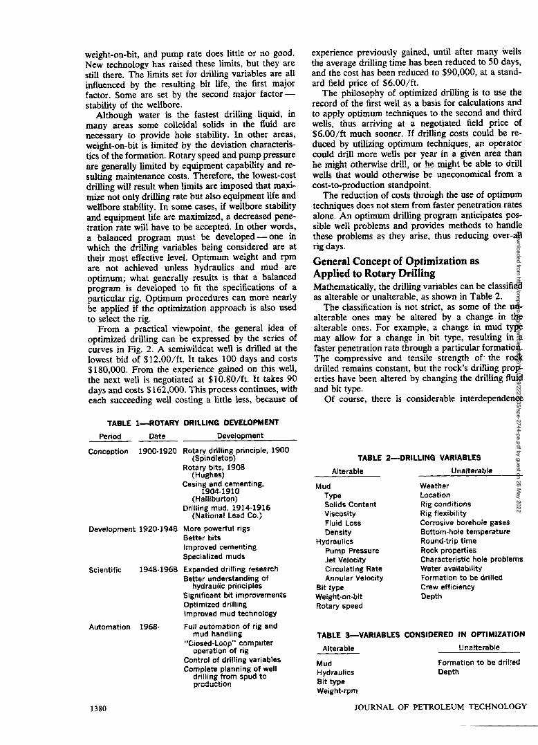
to 1920; Development Period —1 920 to 1948; Scien-tific Period — 1948 to 1968; and Automation Period,which began in 1968. The major accomplishments ofthe first three periods, and a prediction of what liesin the future for the Automation Period are shownin Table 1.

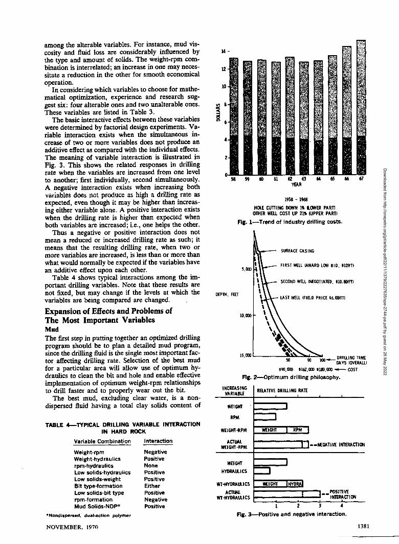
In reviewing these development periods, the ques-tion naturally arises as to the reason for the approx-imate 30-year lapse between the end of the ConceptionPeriod and the start of the Scientific Period. Thereare a number of reasons that can be given, but un-d~~btedly the most significant is that major oilfieldequipment firms, mud service companies, and opera-tors did not start appropriating the large amounts ofmoney it takes to do high-quality drilling researchuntil about 1948. When we look at the major accom-plishments of the Scientific Period, the most produc-tive years are found to be from 1958 to 1968. Ameasure of the impact of the drilling technologydeveloped during the latter part of the ScientificPeriod on homemaking costs, as compared with totalwell costs, can be seen from Fig. 1.

Total well costs increased 14 percent from 1958through 1967, but homemaking costs remained at the1958 level; i.e., about $4.25 /ft.’ Other costs suchas completion, logging, and casing expenditures in-creased 21 percent. It is estimated that if the extensivedrilling research effort of the past 10 years had not

been undertaken and had not been successfully re-duced to practice in routine drilling operations, atypical 8,000- to 9,000-ft hole would cost an addi-tional $3.00/ft to drill today. This would amount to asavings of approximately $500 million for 1967 alone,which is testimony that the investment in drillingresearch undertaken by many companies has paid off.

Optimized drilling has been one of the most signi-ficant accomplishments of the Scientific Period, butit was not introduced comprehensively until 1967,and therefore will not reach its full potential forseveral years. It is important to realize that optimizeddrilling would not be possible today without the hardwork of numerous researchers who have spent con-

,..sicierame time w.iuyiilg th~ ~,~--t- 0.-. ..-..=- --- -1-.: --+ d ATN.,2 f drilling vari~bles

and how they relate to each other.

Definition and Philosophy of OptimizationThere is no such thing as a “true” optimum drillingprogram; invariably compromises must be made be-cause of limitations beyond our control that result insomething less than optimum. Perhaps it can be ex-plained this way: for years it has been known thatrate of penetration could be increased by drillingwith water, by rotating the bit faster, and by increasingflow velocity through jets in the bit. Lack of sufficientmechanical and hydraulic horsepower, however, oftenprevents the proper balancing of variables to obtainmaximum drilling efficiency. Also, there has alwaysbeen a limiting value over which an increase in rpm,

Optimized drilling techniques, first applied in 1967, have significantly reduceddrilling costs, but have not yet reached full potential. Detailed treatment is givento the interactions oj the most important drilling variables. Results indicate thatbetter data, more experience, and confidence will result in greater savings in the future.

NOVEMBER, 1970 ~—~r 1379

Dow

nloaded from http://onepetro.org/jpt/article-pdf/22/11/1379/2227635/spe-2744-pa.pdf by guest on 26 M

ay 2022

weight-on-bit, and pump rate does little or no good.New technology has raised these limits, but they arestill there. The limits set for drilling variables are allinfluenced by the resulting bit life, the first majorfactor. Some are set by the second major factor —stability of the wellbore.

Although water is the fastest drilling liquid, inmany areas some colloidal solids in the fluid arenecessary to provide hole stability. In other areas,weight-on-bit is limited by the deviation charactens-~c~ of ~heformation. Rotary speedand pump pressureare generally limited by equipment capability and re-sulting maintenance costs. Therefore, the lowest-costdrilling will result when limits are imposed that maxi-mize not only drilling rate but also equipment life andwellbore stability. In some cases, if wellbore stabilityand equipment life are maximized, a decreased pene-tration rate will have to be accepted. In other words,a balanced program must be developed — one inwhich the drilling variables being considered are attheir most effective level. Optimum weight and rpmare not achieved unless hydraulics and mud areoptimum; what generally results is that a balancedprogram is developed to fit the specifications of aparticular rig. Optimum procedures can more nearlybe applied if the optimization approach is also usedto select the rig.

From a practical viewpoint, the general idea ofoptimized drilling can be expressed by the series ofcurves in Fig. 2. A serniwildcat well is drilled at thelowest bid of $ 12.00/ft. It takes 100 days and costs$180,000. From the experience gained on this well,the next well is negotiated at $ 10.80/ft. It takes 90days and costs $162,000. Thk process continues, witheach succeeding well costing a little less, because of

TABLE l—ROTARY DRILLING DEVELOPMENT

Period Date

Conception 1900-1920

Development 1920-1948

Scientific 1948-1968

Automation 1968-

1380

Development

Rotary drilling principle, 1900(Spindletop)

Rotary bits, 1908(Hughes)

Casing and cementing,1904-1910

(Halliburton)Drilling mud, 1914-1916

(Natioriai Lead Cc.)

More powerful rigsBetter bitsImproved cementingSpecialized muds

Expanded drilling researchBetter understanding of

hydraulic principlesSignificant bit improvementsOptimized drillingImproved mud technology

Full automation of rig andmud handling

‘‘t30se&Loop” computeroperation of rig

Control of drilling variablesComplete planning of well

drilling from spud topi~dti~~.~fl

experience previously gained, until after many wellsthe average drilling time has been reduced to 50 days,and the cost has been reduced to $90,000, at a stand-ard field price of $6.00/ft.

The philosophy of optimized drilling is to use therecord of the first well as a basis for calculations andto apply optimum techniques to the second and thirdwells, thus arriving at a negotiated field price of$6.00/ft much sooner. If drilling costs could be re-duced by utilizing optimum techniques, an operatorcould drill more wells per year in a given area thanL“e ~g~t othe,%~isedrfl!, or he might be able to d~lwells that would otherwise be uneconomical from ‘acost-to-production standpoint.

The reduction of costs through the use of optimumtechniques does not stem from faster penetration ratesalone. An optimum drilling program anticipates pos-sible well problems and provides methods to handlethese problems as they arise, thus reducing over-allrig days.

General Concept of Optimization asApplied to Rotary DrillingMa&ematically, the drilling variables can be classifiedas alterable or unalterable, as shown in Table 2.

The classification is not strict, as some of the un-alterable ones may be altered by a change in thealterable ones. For example, a change in mud typemay allow for a change in bit type, resulting in afaster penetration rate through a particular formation.The compressive and tensile strength of the rockdrilled remains constant, but the rock’s drilling prop-erties have been altered by changing the drilling fluidand bit type.

Of course, there is considerable interdependence

TABLE 2—DRILLING VARIABLES

Alterable Unalterable

MudTypeSolids ContentViscosityFluid LossDensity

HydraulicsPump PressureJet VelocityCirculating RateAnnular Velocity

Bit typeWeight-on-bitRotary speed

WeatherLocationRig conditionsRig flexibilityCorrosive borehoie gasesBottom-hole temperatureRound-trip timeRock propertiesCharacteristic hole problemsWater availabilityFormation to be drilledCrew efficiencyDepth

TABLE 3-VARIABLES CONSIDERED IN OPTIMIZATION

Alterable I lnaltcimb!~“,, ”,----

Mud Formation to be dril!ed

Hydraulics Depth

Bit typeWeight-rpm

JOURNAL OF PETROLEUM TECHNOLOGY

Dow


ay 2022

among the alterable variables. For instance, mud vis-cosity and fluid loss are considerably irdluenced bythe type and amount of solids. The weight-rpm com-bination is interrelated; an increase in one may neces-sitate a reduction in the other for smooth economicaloperation.

In considering which variables to choose for mathe-matical optimization, experience and research sug-gest six: four alterable ones and two unalterable ones.These variables are listed in Table 3.

The basic interactive effects between these variableswere determined by factorial design experiments. Va-riable interaction exists when the simultaneous in-crease of two or more variables does not produce anadditive effect as compared with the individual effects.The meaning of variable interaction is illustrated inFig. 3. This shows the related responses in drillingrate when the variables are increased from one levelto another; first individually, second simultaneously.A negative interaction exists when increasing both.._.: =l_l_- A-... -,.. -.aA,.,..a ~= ~i.h n t-k~~g ~~f~ ~SVarldolcs Uucs Ilul p Uuu-w a. 1 A&. - --

expected, even though it may be higher than increas-ing either variable alone. A positive interaction existswhen the driliing rate is higher than expected wheiiboth variables are increased; i.e., one helps the other.

Thus a negative or positive interaction does notmean a reduced or increased drilling rate as such; itmeans that the resulting drilling rate, when two ormore variables are increased, is less than or more thanwhat would normally be expected if the variables havean additive effect upon each other.

Table 4 shows typical interactions among the im-portant drilling variables. Note that these results arenot fixed, but may change if the levels at which thevariables are being compared are changed.

Expansion of Effects and Problems ofThe Most Important VariablesMudThe fist step in putting together an optimized drillingprogram should be to plan a detailed mud program,since the drilling fluid is the single most important fac-tor affecting drilling rate. Selection of the best mudfor a particular area will allow use of optimum hy-draulics to clean the bk and hole and enable effectiveimplementation of optimum weight-rpm relationshipsto drill faster and to properly wear out the bit.

The best mud, excludkg clear water, is a non-dispersed fluid having a total clay solids content of

TABLE &TVPICAL DRILLING VARIABLE INTERACTIONIN HARD ROCK

Variable Combination Interatiion

Weight-rpm Negative

Weight-hydraulics Positiverpm-hydraulics NoneLow solids-hydraulics PositiveLow solids-weight PositiveBit type-formation EitherLow solids-bit type Positiverpm-formation NegativeMud Solids-NDP* Positive

●Nondispemed, dual-action polymer

NOVEMBER, 1970

14-

3S3960616263U65 6667YEAR

195s- 196s

HOLECUTTINGGCWN1%EL(WERPART)OTHERWELLCOSTUP 21%IUPPERPART)

Fig. l—Trend of industry drilling coats.

DEPTH,kSURFACECASING

1 FIRST WfLL (AWARDLCW BID, $12FFT)5,UID

t\ SECONDWELL (tWGOTIATEtI,$10.W~)In

FEET

k

\ LAST WELL (FIELD PRICE $6.OWtT)

\\10,OOO ,

\

“$,

*+15,W0

SD 90 ~m_ DRILLING TIMEMYS (OVERALLI

$W,000 $162,0LlT$lSO,GIO— COST

Fig. 2-Optimum drilling philosophy.

INCREASINGVARIABLE RELATIVEGRIUINGRATE

1

WEIGHT

RPM

WEIGHT4PM

ACTUALWEIGH7-RPMEWEIGH7 RPM

--NEMTIVE INTERACTION

‘E’”FHYORAIAICS

fig. 3-Positive and negative interadlon.

1381

Dow


ay 2022

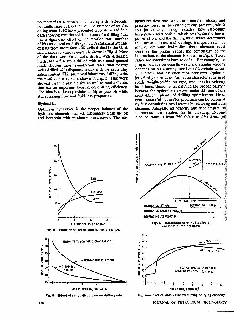
no more than 4 percent and having a drilled-solids:bentonite ratio of less than 2:1.2 A number of articlesdating from 1960 have presented laboratory and fielddata showing that the solids content of a drilling fluidhas a significant effect on penetration rate, numberof bhs used, and on drilling days. A statistical averageof data from more than 100 wells drilled in the U. S.and Canada to various depths is shown in Fig. 4. Mostof the data were from wells drilled with dispersedmuds, but a few wells drilled with true nond@ersedmuds showed faster penetration rates than nearbywells drilled with dispersed muds with the same claysolids content. ~hk prompted hiboraterj driliirrg tests>

-..1..1 4 ,the results “L wk. ------

.Ph a% ~~om in Fig. 5. This work

showed that the particle size as well as total colloidalsize has an important bearing on drilling efficiency.The idea is to keep particles as big as possible whilestill retaining flow and fluid-loss properties.

Hydraulics

Optimum hydraulics is the proper balance of thehydraulic elements that will adequately clean the bitand borehole with filmum horsepower. The ele-

~jIs

PERCENT SOLIDS BY VOLUME

Fig. 4-Effect of solids on drilling performance.

95

h EENTONIT~TOLOWYIFLDCLAYRATlOkl

g903

6s --- *1 z 3 4 6

SIXIDS CONTENT,VOLUME%

Fig. 5-Effect of solids dispersion on drilling rate.

ments are flow rate, which sets amular velocity andpressure losses in the system; pump pressure, whichsets jet velocity through nozzles; flow rate-pumphorsepower relationship, which sets hydraulic horse-power at bit; and the drilling fluid, which determinesthe pressure losses and cuttings transport rate. Toachieve optimum hydraulics, these elements mustwork in the proper ratios; the complexity of theinteractions of the elements is shown in Fig. 6. Theseratios are sometimes hard to define. For example, theproper balance between flow rate and annular velocitydepends on bit cleaning, erosion of borehole in tur-bulent flow, and lost circulation problems. optimum. ---- -~ .mfi+-~.tipc nll~djet velocity depends on rormatiorI ~i,a,~~-...”.., ...soiids, weight-on.~i~, bit type,and annular velocity

limitations. Decisions on defining the proper balancebetween the hydraulic elements make thk one of themost difficult phases of drilling optimization. How-ever, successful hydraulics programs can be preparedby first considering two factors: bit cleaning and holecleaning. Adequate jet velocity and fluid impact ormomentum are required for bit cleaning. Recom-mended range is from 250 ft/sec to 450 ft/sec jet

#’-l’-lMAXIMUNETs lM~ACT

““””%/

SYSTEM LOSSES

I 1

FLW RATE.GPM —

INCREASINGJ~ HttP DECREASINGJETHHP.INCREASINGANNLLARVELOCITY

DECREASINGJETVELOCITY

Fig. 6-interrelations of hydraulics atconstant pump pressure.

Sr.lr

To -

KI -

50 -

4D -

30 -l/2 x 1/4 CUTTING IN 12-U4“ HOLE

20 - ANNULAR VELOCITY .90 F1/MIN

10

0 , , , , t , ,o~;

YIELD VALUE, LB/100 IT.z

Fig. 7—Effect af yield ve!ix+ orr cutting carrying capacity.

JOURNAL OF ?ETROLEUM TEKHNQI.-QGY1382

Dow


ay 2022

velocity as drilling rate varies from 5 to 100 ft/hr.Guidelines to obtain adequate fluid impact vary from73 percent hydraulic horsepower at bit during thefast upper-hole drilling to 49 percent during slowerdrilling at greater well depths.

In hole ~l~~m;mothe r-nest important consideration“.”..l . ...~. ---- ---is to have a mud with sutlicient yield value to liftcuttings from the hole. Results of cutting lifting tests(Fig. 7) indicate that a yield value above the 4 to 6range does not significantly improve the abflity ofdrilling fluid to remove cuttings.’ An adequate an-nular velocity depends on hole size and on the yieldvalue of the mud system. These values should beadjusted together for the following reasons: (1) tomaintain the yield value as low as possible to facilitatesettling of small cuttings in surface pits; (2) to keepve!ocity and cutting transport rate reasonably closein value; and (3) to assure that the annular flowpattern is neither in extreme turbulence nor in totalplug flow.

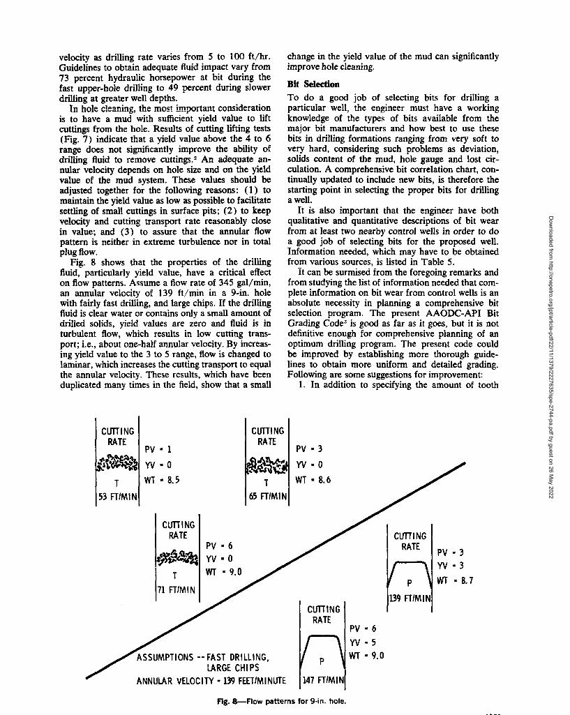
Fig. 8 shows that the properties of the drillingfluid, particularly yield value, have a critical effecton flow patterns. Assume a flow rate of 345 gal/rein,an annular velocity of 139 ft/min in a 9-in. holewith fairly fast drilling, and large chips. If the drillingfluid is clear water or contains only a small amount ofdrilled solids, yield values are zero and fluid is inturbulent flow, which results in low cutting trans-port; i.e., about one-half annular velocity. By increas-ing yield value to the 3 to 5 range, flow is changed tolaminar, which increases the cutting transport to equalthe annular velocity. These results, which have beenduplicated many times in the field, show that a small

change in the yield value of the mud can significantlyimprove hole cleaning.

Bit Selection

To do a good job of selecting bits for drilling aparticular well, the engineer must have a workhgknowledge of the types of bits available from themajor bit manufacturers and how best to use thesebits in driiling formations ranging from very soft tovery hard, considering such problems as deviation,solids content of the mud, hole gauge and lost cir-culation. A comprehensive bit correlation chart, con-tinually updated to include new bits, is therefore thestarting point in selecting the proper bits for drillinga well.

It is also important that the engineer have bothqualitative and quantitative descriptions of bit wearfrom at least two nearby control wells in order to doa good job of selecting bits for the proposed well.Information needed, which may have to be obtainedfrom various sources, is listed in Table 5.

it can ‘besurmised from the foregoing remarks andfrom studying the list of information needed that com-plete information on bit wear from control wells is anabsolute necessity in planning a comprehensive bitselection program. The present AAODC-API BitGrading Code’ is good as far as it goes, but it is notdefinitive enough for comprehensive planning of anoptimum drilling program. The present code couldbe improved by establishing more thorough guide-lines to obtain more uniform and detailed grading.Following are some suggestions for improvement:

1. In addition to s~cif ying the amount of tooth

Pv=l

Yv=o

WT =8.5

CUTTINGRATE

I&#j-$

T

j5 FT/Ml h

PV”3

Yv=o

WT -8.6

1CUlllNGRATE

~;*4 ;:;

WT = 9.0~ W*3

T

H

P WT = 8.771 FT/MIN

/d

139 HIMI NCLllllNG

RATEPV=6

YV=5

ASSUMPTIONS -- FAST DRILLING, WT = 9.0

/LA!?(% 0-!1 %

ANNULAR VELOCITY -139 FEET/Ml NUTE [M7;IMINI

Fig. 8-Flow patterns for 9-in. hole.

NOVEMBER, 1970 1383

Dow


ay 2022

wear, criteria should be provided to indicate whichteeth should be measured to obtain the grading fora given bit type.

2. Guidelines should be developed for measuringthe remaining useful tooth life; this could be a pro-cedure similar to the one presently used to estimateremaining bearing life.

3. Bits pulled because they have reached an eco-nomic limit as a result of formation changes or lossin penetration rate, or for other reasons such as be-coming “plugged”, should be so noted.

4. Insert-type bits should be graded in terms ofwear caused by feet of hole made at specified weightand rotary speeds rather than in terms of repair-ability.

5. Any abnormal wear such as number of brokenteeth and position of these broken teeth on the bitshould be so noted.

These, and possibly other suggested guidelines,~o.~d & in~~rp~rated into the present bit-gradingcode without undue complication of the gradingprocedure and would provide more uniform gradingthroughout the industry. An improved bit-gradingcode would make it possible to obtain better datafor more skillful planning.

Weight-rpm

Pan American’s optimized drilling program is basedon equations developed by Galle and Woodss andBillington and BlenkamG, which define how the com-plex relationship between weight-on-bit and rpm

TABLE *BIT WEAR INFORMATION REQUIRED FOROPTIMIZED DRILLING PROGRAM

Mill Tooth Bits

Economic life remaining (teeth and bearings)Tooth heightGauge wear

Type of weem

Abnormal wear

Failures:

Insert Bits

Bearings

Self sharpeningFlat e restedBroken teethChipped teethUpset teeth

Shirt-tail wearTrackingInner-row teeth gone and

heel rows goodNose bearing looseOff-center wear

Broken conesBroken spearpointCones lockedSeal failurepinchedCoring

Economic iife remaining

Cutth’rg structure (repairability of conas indicated,1 through 4):

l—All cones repairable2—Two cones repairable3-One cone repairable4-All cones worn beyond

1384

repair

affects the wear of a bit in a particular formation. Toget some concept of optimization, it is important tounderstand what these equations can provide in termsof data output. Using these equations, the weight:rotary-speed relationship can be categorized as fol-lows :

Variable rpm-weight. Because so few rigs are electricor completely versatile as far as range of rpm andweight is concerned, little use can be made of a vari-able optimum rpm and weight program. However, itis the most efficient method for drilling with milltooth bits.

Constant rpm-Variable Weight. This method for &Ill-ing with mill tooth bits appears to be practical. Gen-erally, good drillers gradually apply more weight asbits become dull. This method has not been widelyaccepted since it requires an automatic driller andmore supervision than other weight-rpm programs.-- the Constant rpm andHowever, vdier& app!icabh% ....variable weight method is considerably more eflicientthan constant rpm and constant weight programs.

Constant rpm and Weight. Because of the limitationsindicated above, most computer programs have beenrestricted to constant rpm and weight. i3eca-use somany limitations do exist, it has been necessary tomake programs as flexible as possible and to coveras wide a range as the drilling engineer considersnecessary. There are three available approaches.

1. O~th&% ?~.rn !2.?UiWeight. This is the rpmand weight that one might run if no limitations exceptthe bit could be considered. This is the rpm andweight for absolute minimum cost, not consideringany other factors such as condition of drill string,deviated hole or development of torque.

2. Best Weight for Given rpm. Should formationor rig capability limit rpm, the program will determinethe proper weight for minimum cost with imposedrestrictions. This will cost more per foot than when

.“ + -** ,,C(WIoptimum rpni and ‘weiw!L~ ~ .=...3. Best rpm for Given Weight. Should the avail-

able drill collars or deviation control dictate a certainweight-on-b]t, this program predicts proper rpm foroptimum cost considering this restriction. This costwill also be more than for optimum rpm and weight.

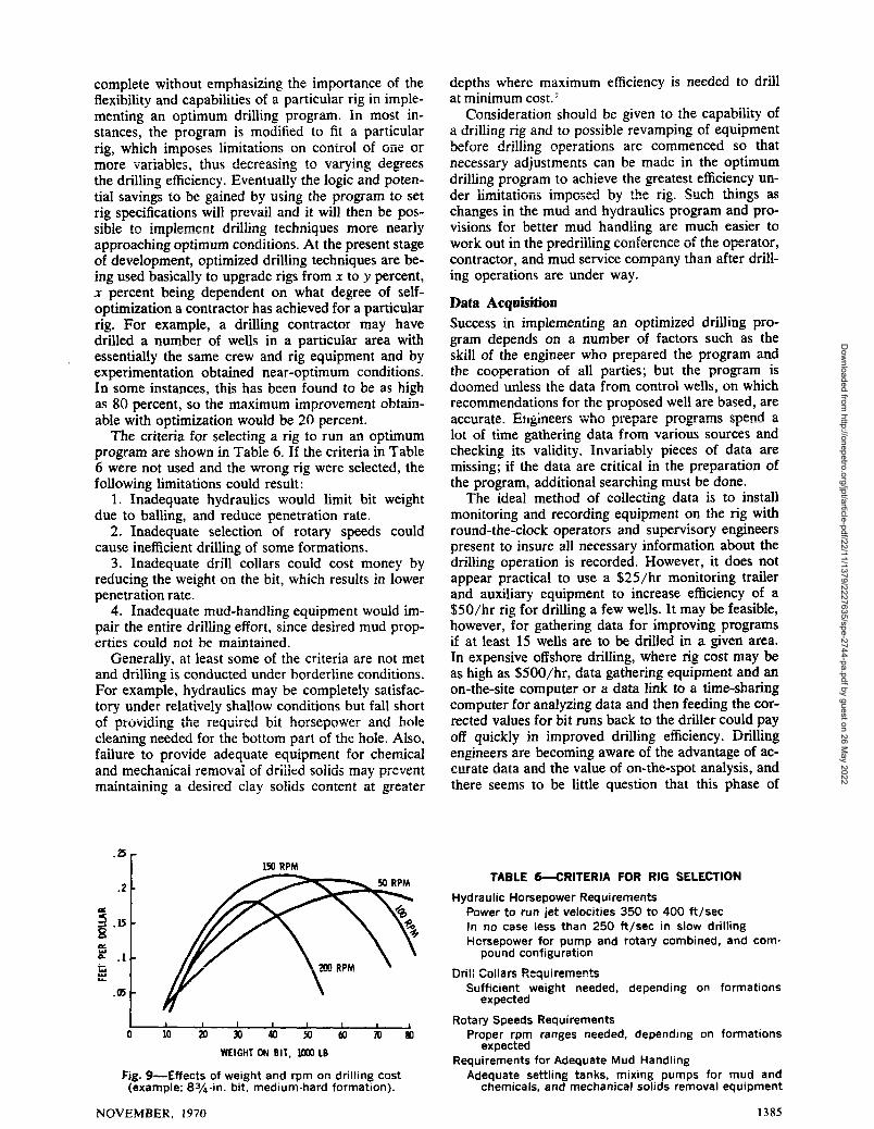
Fig. 9 shows an example of how optimum drilkgprograms select the proper weight and rpm to achieveminimum-cost drilling. In this instance, a medium-hard formation is being drilled with an 8%-in. milltooth bit “inside the computer” at varying weights~-ld ic~&~Y~speeds. The data show that a combinationof 150 rpm and 45,000 lb weight-on-bit would drillthis particular formation at the lowest cost. The nextbest combination would be 100 rpm and 55,000 lbon bit. The advantage of the computer is that equa-tions can be quickly and economically solved to pro-vide information, such as show-ii in Fig. 9, for r!multiple number of conditions. This provides thedriller with a flexibility that he never had before.

Rig !kkction

No discussion on drilling optimization would be

JOURNAL OF PETROLEUM TECHNOLOGY

Dow


ay 2022

complete without emphasizing the importance of theflexibility and capabilities of a particular rig in imple-menting an optimum drilling program. In most in-stances, the program is modified to fit a particularrig, which imposes limitations on control of ofie ~i

*L.-. d~m-encinu to v~rying degreesmore ~arkdie~, Lllu. u----- Ha

the drilling efficiency. Eventually the logic and poten-tial savings to be gained by using the program to setrig specifications will prevail and it will then be pos-sible @ irnp!e-rn.ent drilling techniques more nearlyapproaching optimum conditions. At the present stageof development, optimized drilling techniques are be-ing used basically to upgrade rigs from x to y percent,x percent being dependent on what degree of self-optimization a contractor has achieved for a particularrig. For example, a drilling contractor may havedrilled a number of wells in a particular area withessentially the same crew and rig equipment and byexperimentation obtained near-optimum conditions.In some instances, this has been found to be as highas 80 percent, so the maximum improvement obtain-able with optimization would be 20 percent.

The criteria for selecting a rig to run an optimumprogram are shown in Table 6. If the criteria in Table6 were not used and the wrong rig were selected, thefollowing limitations could result:

1. Inadequate hydraulics would limit bit weightdue to balling, and reduce penetration rate.

2. Inadequate selection of rotary speeds couldcause ineiiicient drilling of some formations.

3. Inadequate drill collars could cost money byreducing the weight on the bit, which results in lowerpenetration rate.

4. Inadequate mud-handling equipment would im-pair the entire drilling effort, since desired mud prop-erties could not be maintained.

Generally, at least some of the criteria are not metand drilling is conducted under borderline conditions.For example, hydraulics may be completely satisfac-tory under relatively shallow conditions but fall short

r .-fi..:.-~ h;t hnr.ennw~~ ~~(j ~ole01 p~O~k@ d’i& lGLtUIl w u.. ..”. .-y V..

cleaning needed for the bottom part of the hole. Also,failure to provide adequate equipment for chemicaland mechanical removai of ciriiied ~~iid~inay preventmaintaining a desired clay solids content at greater

depths where maximum efficiency is needed to drillat minimum cost. ~

Consideration should be given to the capability ofa drilling rig and to possible revamping of equipmentbfnre ~ril]ino nneratjon5 are commenced so thatl-n,, ”,” u. . . . . . . -r-.—.

necessary adjustments can be made in the optimumdrilling program to achieve the greatest et%ciency uti-der ihnitatioiis imposed byy the rig. Such things aschanges in the mud and hydraulics program and pro-visions for better mud handling are much easier to

. .,, .work out in the prearllung conferen@ d the G~~ratOT,

contractor, and mud service company than after drill-ing operations are under way.

Data Acquisition

Success in implementing an optimized drilling pro-gram depends on a number of factors such as theskill of the engineer who prepared the program andthe cooperation of all parties; but the program isdoomed unless the data from control wells, on whichrecommendations for the proposed well are based, are

...~- ~..~ .- ~r ornmq snend aaccurate. Etigt~&iS WIIV ~1 ~Pal. ~lo=. ----- -r -...lot of time gathering data from various sources andchecking its validity. Invariably pieces of data aremissing; if the data are critical in the preparation ofthe program, additional searching must be done.

The ideal method of collecting data is to installmonitoring and recording equipment on the rig withround-the-clock operators and supervisory engineerspresent to insure all necessary information about thedrilling operation is recorded. However, it does notappear practical to use a $25 /hr monitoring trailerand auxiliary equipment to increase efficiency of a$50/hr rig for drilling a few wells. It maybe feasible,however, for gathering data for improving programsif at least 15 wells are to be drilled in a given area.In expensive offshore drilling, where rig cost may beas high as $500/hr, data gathering equipment and anon-the-site computer or a data link to a time-sharingcomputer for analyzing data and then feeding the cor-rected values for bit runs back to the driller could payotl quickly in improved drilling efficiency. IMiitigengineers are becoming aware of the advantage of ac-curate data and the value of on-the-spot analysis, andthere seems to be little question that this phase of

1S0RPMTABLE MRITERIA FOR RIG SELECTION

Hydraulic Horsepower RequirementsPower to run jet velocities 350 to 400 ft/secIn no case less than 250 ft/sec in slow drillingHorsepower for pump and rotary combined, and com-

pound configuration

Y

m-:,, F 11 .= me. ,,i.amantcurlll uOtiaI= I.=q Uo.e,, o-----Sufficient weight needed, depending on formations

expected

I I 1 I 1 1 I Rotary Speeds Requirements1 40 102030405060 7080 Proper rpm ranges needed, depending on formations

WEIGHTON BIT, KK81LB expected

Requirements for Adequate Mud HandlingFig. 9—Effects of weight and rpm on drilling cost Adequate settling tanks, mixing pumps for mud and

(example: 8s~-in. bit, medium-hard formation). chemicals, and mechanical solids removal equipment

NOVEMBER, 1970 1385

Dow


ay 2022

drilling will expand greatly in the near future.On a less sophisticated but more practical level,

Pan American has found since 1966 that effectiveoptimized drilling programs can be prepared usirighand-recorded data from the AAODC-API dailydrilling reports, mud service company mud reports,and bit records, augmented with information fromlogs and discussions with drilling contractors. Thisdata collection procedure will continue for some timeto supply information needed to optimize most ofour wells. Improved industry standard forms, suchas the Daily Drilling Report, coded to facilitate key-punching, will not only reduce the amount of writinga driller has to do but also upgrade what he doeswrite. Wide use of these forms will soon result inbetter records.

The data required to prepare an optimized drillingprogram are listed in Table 7.

Field Application of OptimizedDrilling ProgramsThere have been many problems encountered in im-plementing optimized drilling programs, These pro-grams suggest changes in past drilling techniques —changes involving mud system, drilling assembly, riggeometry, bit types, and hydraulics. Some contractorsare accustomed to drilling on experience only, andare naturally reluctant to change their techniques untilthey see that optimized drilling programs are an im-provement over present practices. A number of con-tractors have now had considerable experience withoptimized drilling techniques and several are com-pletely sold on the advantages arid potential of this- ---~-:~1:-- n=-r arhnew ULIU1115 ~pyle-...

Another important problem with these programsdevelops when rig equipment is not the same as thaton which the program was based. This difference inrig equipment can have an effect on the weight-rpmprogram, the hydraulics program, and the mudprogram.

Many problems can develop after the drillingprogram has been started. Formation tops may bedifferent from those in the program, bit performancemay be much lower than expected, pump pressure~lzY be IQwcr than planned, or well “kicks” may re-quire premature weighting-up of the mud.

To prevent problems that are almost sure to arisefrom se~,@ti~yY,di~IuPting [email protected], the drilling

optimization program should be planned to have asmuch flexibility as possible. The drilling recommenda-.,tions can be cnanged to fit the rig eq’~pm..-. . ..Pnt and thenrerun through the computer. Also, equipment can be

1.2.3.4.

5.

647

TABLE 7—DATA REQUIRED FORDRILLING OPTIMIZATION

Logs (preferably IES or sonic)Bit recordsMud records

Recorded drilling data: torque, pump pressure, pene-tration rater etc.Drilling specifications for proposed well: casing points,hole size, expected problems, etc.Rig specificationsCorrelation of formation tops to proposed well

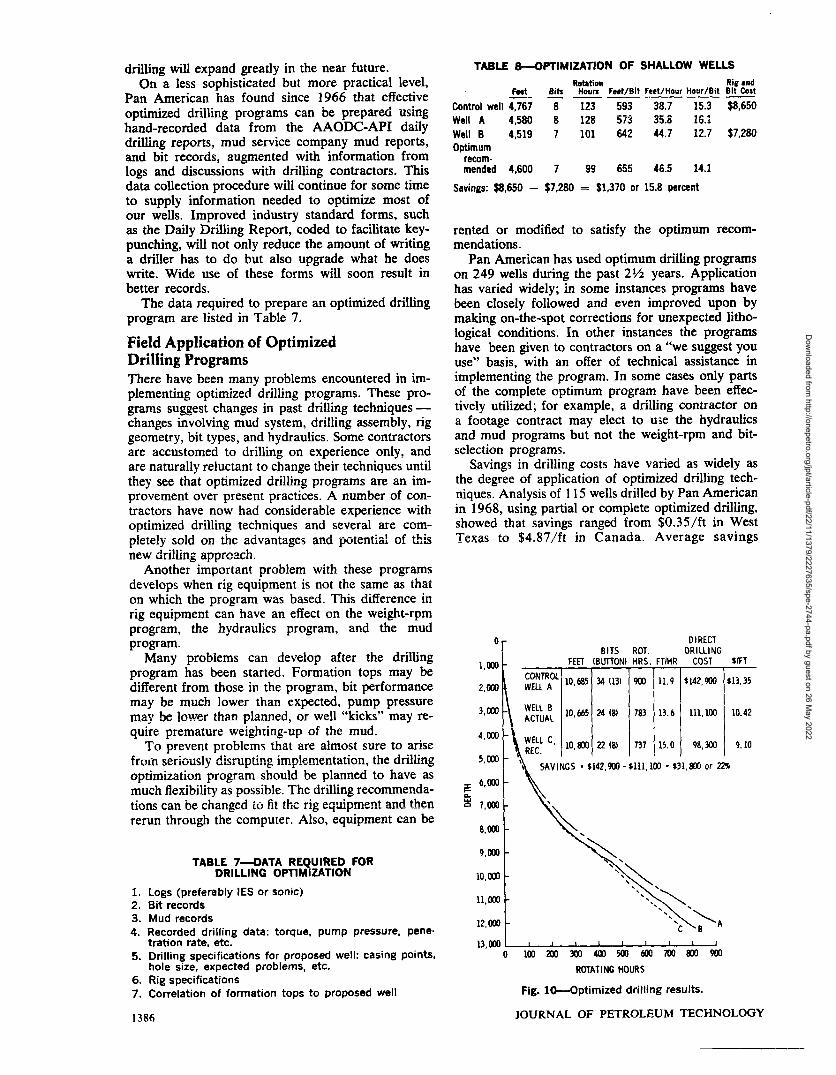
TABLE B--OPTIMIZATION OF SHALLOW WELLS

Bib Rotetion Rig mdFact Howe Feet/Bit Feet/Hour Hour/Bit Bit Cost—— —— —

Control well 4,767 8 123 593 38.7 15.3 $8,650Well A 4,580 8 128 573 35.~ i&. i

Well B 4,519 7 101 642 44.7 12.7 $7,280Optimum

recom-mended 4,600 7 99 655 46.5 14.1

Savings: $8,650 – $7,280 = $1,370 or 15.8 percent

rented or modified to satisfy the optimum recom-mendations.

Pan American has used optimum drilling programson 249 wells during the past 2%2 years. Applicationhas varied widely; in some instances programs havebeen closely followed and even improved upon bymaking on-the-spot corrections for unexpected litho-logical conditions. In other instances the programshave been given to contractors on a “we suggest youuse” basis, with an offer of technical assistance inimplementing the program. In some cases only partsof the complete optimum program have been effec-tively utilized; for example, a drilling contractor ona footage contract may elect to uje the hydraulicsand mud programs but not the weight-rpm and bit-selection programs.

Savings in drilling costs have varied as widely asthe degree of application of optimized drilling tech-niques. Analysis of 115 wells drilled by Pan Americanin 1968, using partial or complete optimized drilling,showed that savings ranged from $0.35 /ft in WestTexas to $4.87/ft in Canada. Average savings

‘r DIRECT

BITS ROT. DRILLING

l,OW

I

FEEI (BUTTON) HRS. FTIHR COST $IFT

2,0ik3gJ~AoL 10,685 34 (13) WI 11.9 $142, KM $13.35

3#Lm ~#u:L 10,6b5 24 (81 7s3 13.6 111,lW 10.42

4,cw

~\

;Ey c‘ 10,800 22 (8) 737 15.0 98,3W 9.10

5,000 ,SAVINGS . $142,903- $lll,lm = $31,SW or 2.2%

~ 6,030

hm 7,000 [

8,000 -

9,ao -

10,OW -

Il,ooo -

12,0m -

n,mo~lm2003004m 5m60070fJm09m

ROTATING HOURS

Fig. 10-Optimized drilling results.

JOURNAL OF PETROLEUM TECHNOLOGY1386

Dow


ay 2022

Well

A

BABAB

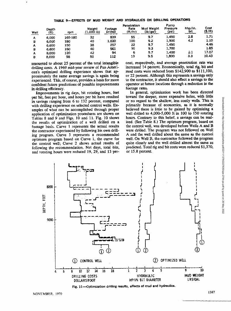
TABLE 9-EFFECTS OF MUD

Depth Weight(ft) rpm (1,000 lb)

6,000 160-180 326,000 180 406,600 150 386,600 160 &e8,000 120 428,000 98 50

WEIGHT AND HYDRAULICS ON DRILLING OPERATIONS

FootageDrilled

8391,030

257~~~

94112

~QImtecI to about 25 percent of the total intangibledrilling costs. A 1969 mid-year review of Pan Anieri-can’s optimized drilling experience shows that approximately the same average savings is again beingexperienced. This, of course, provides a basis for moreconfident future predictions of possible improvementsin drilling efficiency.

Improvements in rig days, bit rotating hours, feetper bit, feet per hour, and hours per blt have resultedin savings ranging from 6 to 132 percent, comparedwith drilling experience on selected control wells. Ex-amples of what can be accomplished through properapplication of optimization procedures are shown onTables 8 and 9 and Figs. 10 and 11. Fig. 10 showsthe results of optimization of a well drilled on afootage basis. Curve 1 represents the actual resultsthe contractor experienced by following hk own drill-ing program. Curve 3 represents a recommendedoptimum program based on Curve 1, the curve forthe control well; Curve 2 shows actual results offollowing the recommendation. Net days, total bits,and rotating hours were reduced 19, 29, and 13 per-

Ik---- —-- ----- 3

penetration PumpRate Mud Waight Pressure bhp/in. cost

(ft/hr) (lb/gal) (psi) bit ($/ft)—.

55 9.7 1,450 2.8 1.71100 9.2 1,900 4.2 1.10

22 9.7 1,450 4.4630 9.3 1,700 1.85

6 9.7 1,400 2.1 17.0713 9.5 1,800 3.3 10.43

cent, respectively, and average penetration rate wasincreased 14 percent. Economically, total rig, bit andmud costs were reduced from $142,900 to $111,100,or 22 percent. Although this represents a savings onlyto the contractor, it should also effect a savings to theoperator at future locations through a reduction in thefootage rates.

In general, optimization work has been directedtoward the deeper, more expensive holes, with littleor no regard to the shallow, less costly wells. This isprimarily because of economics, as it is normallybelieved there is little to be gained by optimizing awell drilled to 4,000-5,000 ft in 100 to 150 rotatinghours. Contrary to thk belief, a savings can be real-ized. (See Table 8.) The optimum program, based onthe control well, was developed before Wells A and Bwere drilled. The program was not followed on WellA and the well drilled about the same as the controlwell. On Well B, the contractor followed the programquite closely and the well drilled almost the same aspredicted. Total rig and bit costs were reduced $1,370,or 15.8 percent.

I @ CONTROL WELL @ OPTIMIZED WELL

I I 1 I t ! t 1 I 1 I I 1 1 I468 10 12 14 16 18 12345 9 10

!N?!LL!NG COSTS HYDRAULIC MUD WEIGHTDOLLARS/FOOT i-ip/i N EiT i31AiMETER 4BSIGAL

Fig. n-Optimization drilling results, effects of mud and hydraulics.

NO;’E?,4BH?. 1970 1387

Dow


ay 2022

It has been mentioned throughout this paper that.mud and hydrauhcs are two of the mu.. ....F.-a.t imnrsrt~nt

factors affecting the optimization of drilling opera-tions. Without optimum mud and hydraulics theweight-rpm program cannot be fully implemented.Examples showing the effects of these two variablesare in Table 9 and Fig. 11. Table 9 reflects the resultsof selected bit runs from two wells drilled in the.same area m the Rocky Mountain;. Opti,mIza..”.. . .

. .tifin cal-

culations were not prepared for either well since bothare located in an area of fast drilling and relativelylow cost. Well B, however, was drilled with iower-

. . . -..-.. -rs.cllre ~~i~h resultedweight mud ana nqgher PMIIP ~. ~..-.., . . .in better ciosvnhole hydraulics. A comparison of theresults shows that penetration rate and footage perbit were increased to 100 and 118 percent. Drillingcosts per foot, in turn, were reduced 36 to 59 percent.

Fig. 11 reflects similar results but also points outthe detrimental effects of increasing mud weight andsolids content. Shown are the drilling costs by bit~tifi, ~Perating conditions> hvdras.dic horsepower perinch of bit diameter and mu-d weight for the controiwell (Curve 1) and the optimized well (Curve 2).The control well was drilled with a high-weight, high-solids mud and poor down-hole hydraulics. Bit life,penetration rate and feet per bit were quite poor,resulting in high costs per foot. On the other hand,Well 2, the optimized well, employed a low-weight,low-solids mud with considerably better hydraulicsdown to 8,400 ft. In the interval from 8,400 to 9,300ft, however, mud weight increased from 8.7 to 9.9

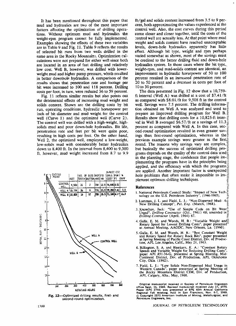
DIRECT CST

;K-

FKT TOOTH BUTT HRS HR COST FT DIFF

7

t\ . .

15} \I

I ,, 1 ! 1 I

lco2J’l~4w-~~zi’

ROTATING iiOiiRS

Fig. 12-Optimized drilling results, first- andsecond-round optimization.

lb/gal and solids content increased from 3.5 to 9 per-cent, both approximating the values experienced at thecontrol well. Also, the cost curves during tim ~...--*T;n~

come closer and closer together, until the costs of thecontrol well are actually less. At that point where mudweight and solids content have reached unacceptablelevels, down-hole hydraulics apparently has littleeffect. Although bit type, weight and rpm perhapsvaried somewhat as shown, most of the savings mustbe credited to the better driiiing fiuid and d~~fi-h~iehydraulics system. In those cases where the bit type,.weight-rpm, and mud-solids content are identical, animprovement in hydraulic horsepower of 50 to 100percent resulted in an increased penetration rrtte of

~ and a decrease in costs per fOOt Of20 to Xl perter.. . ... _10 to 30 percent.

The data presented in Fig. 12 show that a 10,759-ft interval (Well A) was drilled at a cost of $7.41 /ftas compared with $8.01 /ft for 9,508 ft in the controlwell. Savings were 7.5 percent. The drilling informa-tion obtained on Well A was analyzed and used toprepare an ~mpr~~ed drii~ng pro~am for Well B.Results show that drilling costs for a 10,825-ft inter-val in Well B averaged $6.57/ft or a savings of 11.3percent as compared with Well A. In this case, sec-ond-round optimization resulted in even greater sav-ings than first-round optimization, whereas in theprevious example savings were greater in the firstround. The reasons why savings vary are complex,but basically the success of optimized drilling pro-grams depends on the quality of the control data u;edin the planning stage, the confidence that people im-pie,meflting tiie programs have in the principles beingapplied, and the efficiency with which the programsare applied. Another important factor is unexpectedhole problems that often make it impossible to im-plement optimum drilling techniques.

References1.National Petroleum Council Study: “Impact Of New Tech-

nology on the U.S. Petroleum Industry”. (1946-1965).

2. Lummus~ J. L. and Field, L. J.: “Non-Dispersed Mud: ANew Drdling Concept”, Pet. Erzg. (March, 1968).

3. Knowlton, Jack: “Use of Simple Code on Bit WearUrger, Drl~/lrsg C~nirti~~~~ ((k%., !961 ) 68: amended in

. ....

Drilltrrg Contractor (Aprd, 1964) 67.

4. Galle, E. M. and Woods, H. B.: “Variable Weight andRotary Speed for Lowest Drilling Costs”, paper presentedat Annual Meeting, AAODC, New Orleans, La. (1960).

5. Galle, E. M. and Woods, H. B.: West Constard Weigh:and Rotary Speed for Rotary Rock Bits”, paper presentedat Spring Meeting of Pacific Coast District, Div. of Produc-tion, API, Los Angeles, Calif., May 21, 1963.

6. Billington, S. A. and Blenkarn, K. A.: “Constant RotarySpeeds and Variable Weight for Reducing Drilling Costs”,paper API 851 -36-G, presented at Spring Meeting, Mid-Continent District, Div. of Production, API, OklahomaCity, Okla. (1962).

7. Field, L. J.: “Low Solids Non-Dispersed Mud Usage inWestern Canada”, paper presented at Spring Meeting ofthe Rocky Mountain District CIM, Div. of Production,APJ, Calgary, Alta., May, 1968.

Original manuscript received in Society of Petroleum Engineersoffice Sept. 15, 1969. Rewsed manu%, ip, ,=------ .-..--. -b .-.--iv-d Jul” 17, 1970.

Papar (SPE 2744) was presented at SPE 40th Annual California

Regional Fall Meeting, held in San Francisco, NOV. 6-7, 1969.

~ Copyright 1970 American Institute of Mining, Metallurgical, andPet roleum Engineera, Inc.

1388 JOURNAL OF PETROLEUM TECHNOLOGY

Dow


ay 2022

Documents

Drilling Optimization - OnePetro