Durowoju, M 2017.pdf - Newcastle University Theses

i

APPLICATION OF ARTIFICIAL NEURAL NETWORK FOR THE

STRUCTURAL INTEGRITY ASSESSMENT OF DENT IN

PIPELINES

By

MICHAEL OLUWADAMILARE DUROWOJU

A thesis submitted for the degree of Doctor of Philosophy

School of Marine Science and Technology

NEWCASTLE UNIVERSITY

June, 2017

ii

i

ABSTRACT

Dent in a pipelines have been of major concern to pipeline operators for years because

its severity cannot be easily determined. For many years dent severity was based on

dent depth alone. This has led to unnecessary repairs and removal from service

incurring considerable loss in revenue. Studies by researchers have indicated that

other factors like pipe geometry, pipe material, dent geometry and pressure cycling

could influence the severity of the dent in terms of the fatigue life reduction.

Dent severity has been studied using dent depth based assessment, strain based

assessment and fatigue assessment . The dent depth over the years has been the

major determinant of dent severity. Recent studies have shown that the strain in the

pipeline could be a better indicator of dent severity using the static approach. The most

common fatigue approach is the stress life S-N approach. This involves extracting

stress data either through experimental procedure or finite element analysis and using

it with an appropriate S-N curve to determine the fatigue life

One of the major challenges faced in S-N fatigue approach today is determining

the stress concentration factors (SCF) associated with the dents. These SCFs are used

with an appropriate SN curve to calculate the fatigue life. This, over the years and

currently is calculated empirically or using finite element (FE) analysis. The cost of

running experimental program can be very expensive and numerical analysis can be

time-consuming. It is not sustainable to keep using finite element analysis to calculate

the SCF associated with every dent. An algorithm is needed to be able to predict strain

and SCF without running an expensive experimental program or running an extensive

finite element study

This Research presents an alternative and a sustainable method for calculating

the SCF, the maximum strain and the rerounding depth in pipelines with dent. The

method involves gathering a large database of SCFs, strains and rerounding depths

through a finite element study on a parametric range of industry standard pipes . These

parametric datasets focuses on the effects of pipe geometry, dent geometry, material

properties and pressure range on the prediction of the strain and stresses which were

not systematically considered by other researchers. These parametric datasets are

then used to train an artificial neural network (ANN) that predicts the rerounding depth,

ii

maximum strain and the SCF. The ANN presents an accurate and sustainable

alternative to the current method used for dent assessment. It’s application would

reduce the cost and time taken in assessing dent severity. The accuracy of the ANN is

dependent on the amount of training data. In order to create the large database of

results, a parametric design language (APDL) was created for easy creation and

recreation of models. This parametric design language helped in the creation of 256

FE models which was sufficient enough to create the large database of SCF and other

data needed to train the ANN

Two types of indenters (Dome and Bar) are used to simulate circumferentially

and longitudinally aligned dents. Four different dent depths ranging from 2% d/D to

10% d/D are also simulated to investigate the effect of dent geometry. Four different

pipe grades (X46, X65, X80, and X100) are analysed to investigate the effect of pipe

materials. Similarly, eight pipes with a different diameter to thickness ratio (D/t) ranging

from 18-96 are analysed to investigate the effect of pipe geometry. The pipe is

pressured up to 50% and 72% SMYS to investigate the effect of pressure range.

The results from this study show that all the investigated parameters influence

the results in various ways. Results show that longitudinally aligned dents have higher

stress concentrations factors compared to circumferential dents of similar dent depth.

Similarly, pipes with higher diameter to thickness ratios D/t have higher stress

concentration factor compared to pipes with lower D/t .The FE result was validated with

experimental and analytical results and a good correlation was seen with minimal

percentage error. The FE results from the parametric study was fed into an ANN model

to train the network. The network was trained with different numbers of the processing

element and activation function to find the model with the best performance. The ANN

prediction gave a good correlation with the FE results

Keywords:

Finite Element Analysis; Fatigue life; Stress Concentration Factor; Strain-based

assessment; Spring back; Rerounding; Artificial neural network

iii

v

ACKNOWLEDGEMENTS

I thank the Almighty God for the Grace and strength given to me in order to complete

this research.

I am very grateful to my supervisor, Dr Yongchang Pu for his time, guidance and

intellectual resource to making this research a success. I am also thankful to Dr Simon

Benson and Dr Julia Race for their support and advice particularly on the published

papers which is key to this research. My sincere gratitude goes to the entire staff of

School of Marine science and technology for creating an enabling platform and

environment to conducting this research. I also acknowledge the suggestions of my

examiners, Prof Purnendu Das and Dr Nianzhong Chen which helped me to better

highlight the contribution of this thesis.

I am eternally grateful to my parents Chief and Chief Mrs MAO Durowoju for their

prayers, monetary and moral support in making this research a success. Without them,

this dream would have been unachievable

I am very grateful to my wife and son Oluwakemi and Oluwadarasimi for their patience

and understanding. I particular thank my wife for her moral support and fuelling my

drive to achieving this goal

I am also thankful to my brothers Dr Olasunkanmi Durowoju and Dr Olatunde Durowoju

who have set the pace and standard to follow. I am thankful for your monetary and

moral support. You guys are my role models. I am also thankful to younger brother

Oluwatobi Durowoju for his support and prayers. Many thanks to my sisters-in-law,

Tosin, Pretti and Omolola, my nieces, Oyindamola, Zoe and Anika and my nephew

Boluwatife. You guys rock! Many thanks to the entire Durowoju and Olaitan Family for

their prayers

Lastly, I want to thank my friends and colleagues Deji, Ibezimakor, Wale, Charles,

Seun, Dapo, Wunmi, Sammy, Toyosi, Lawunmi, Mary,Tunde and so on for your

support and your kind words of encouragement

vii

viii

TABLE OF CONTENTS

ABSTRACT .......................................................................................................... i

ACKNOWLEDGEMENTS ................................................................................... v

TABLE OF CONTENTS .................................................................................... viii

LIST OF FIGURES ........................................................................................... xii

LIST OF TABLES ............................................................................................ xvi

LIST OF EQUATIONS .................................................................................... xviii

NOMENCLATURE ........................................................................................... xxii

CHAPTER 1 ........................................................................................................ 1

INTRODUCTION ................................................................................................ 1

1.1 General overview ...................................................................................... 1

1.2 Statement of problem ................................................................................ 2

1.3 Aims and Objectives .................................................................................. 3

1.4 Organisation of the thesis .......................................................................... 4

CHAPTER 2 ........................................................................................................ 5

LITERATURE REVIEW ...................................................................................... 5

2.1 Introduction................................................................................................ 5

2.2 History of dent assessment ....................................................................... 6

2.2.1 History of plain dent assessment ................................................................ 6

2.2.2 History of the assessment of dents associated with mechanical damages

............................................................................................................................ 7

2.3 Dent Research ........................................................................... …………9

2.3.1 Static dent research .................................................................................... 9

2.3.2 Dent fatigue research ............................................................................... 13

2.3.3 S-N Approach ........................................................................................... 14

2.3.4 Strain-life Approach .................................................................................. 21

2.3.5 Fracture Mechanics Approach .................................................................. 24

2.3.6 Factors affecting fatigue life assessment of dents .................................... 25

2.3.7 Dent measurement ................................................................................... 28

2.4 Finite element methodology ................................................................... 29

2.4.1 Previous work done using finite element analysis..................................... 30

2.5 Artificial neural network ........................................................................... 31

ix

2.5.1 Neural network architecture ...................................................................... 33

2.5.2 Activation functions ................................................................................... 34

CHAPTER 3 ..................................................................................................... 36

ELASTIC SPRING BACK AND REROUNDING IN DENTED PIPELINE .......... 36

3.1 Introduction ............................................................................................. 36

3.2 Spring back and rerounding mechanism ................................................. 37

3.3 Finite element model ............................................................................... 37

3.3.1 Geometry creation ..................................................................................... 38

3.3.2 Materials .................................................................................................... 40

3.3.3 Elements ................................................................................................... 43

3.3.4 Meshing ..................................................................................................... 47

3.3.5 Boundary conditions .................................................................................. 50

3.3.6 Contact pair creation ................................................................................. 51

3.3.7 Loading ..................................................................................................... 52

3.4 Spring back results ................................................................................. 53

3.4.1 Effect of pipe geometry on spring back ..................................................... 53

3.4.2 Effect of dent geometry on spring back ..................................................... 54

3.4.3 Effect of pipe grade on spring back ........................................................... 55

3.5 Result for rerounding .............................................................................. 56

3.5.1 Effect of pipe geometry on rerounding ...................................................... 57

3.5.2 Effect of dent geometry on rerounding ...................................................... 58

3.5.3 Effect of pipe material on rerounding ........................................................ 59

3.6 Comparison of experimental and finite element model ........................... 61

3.6.1 Spring back validation ............................................................................... 61

3.6.2 Rerounding validation................................................................................ 61

3.7 Summary of result and conclusion .......................................................... 62

CHAPTER 4 ..................................................................................................... 64

FATIGUE ANALYSIS OF PLAIN DENTS USING SN APPROACH .................. 64

4.1 Introduction ............................................................................................. 64

4.2 Current procedure of SN approach ......................................................... 65

4.3 Proposed fatigue analysis procedure ...................................................... 66

4.4 Validation with experimental data ........................................................... 66

4.5 Validation with analytical solution ........................................................... 69

x

4.6 Finite element model ............................................................................... 71

4.6.1 Loading ..................................................................................................... 72

4.6.2 Variables considered ................................................................................ 73

4.6.3 Parametric study ....................................................................................... 73

4.7 Results .................................................................................................... 74

4.7.1 Stress locations ........................................................................................ 74

4.7.2 Effect of pipe geometry on SCF ................................................................ 76

4.7.3 Effect of pipe grade on SCF ..................................................................... 79

4.7.4 Effect of dent geometry on SCF................................................................ 79

4.7.5 Effect of mean internal pressure ............................................................... 80

4.8 Summary of results and conclusions ....................................................... 82

CHAPTER 5 ...................................................................................................... 83

STRAIN-BASED ASSESSMENT OF PLAIN DENTS ....................................... 83

5.1 Introduction.............................................................................................. 83

5.2 Current method for estimating strain in pipeline ...................................... 83

5.3 Finite Element Model ............................................................................... 87

5.3.1 Loading ..................................................................................................... 87

5.3.2 Parametric study ....................................................................................... 87

5.4 Effect of important variables on strain ..................................................... 88

5.4.1 Effect of pipe geometry on strain .............................................................. 92

5.4.2 Effect of dent geometry on strain .............................................................. 94

5.4.3 Effect of pipe grades on strains ................................................................ 95

5.4.4 Comparison between ASME B31.8 , Modified ASME [21] and FEA

predicted strain .................................................................................................. 96

5.5 Summary of results and conclusion ....................................................... 100

CHAPTER 6 .................................................................................................... 103

ARTIFICIAL NEURAL NETWORK APPLICATION FOR PREDICTING

REROUNDING, SCF AND STRAIN IN DENTED PIPELINE .......................... 103

6.1 Introduction............................................................................................ 103

6.2 Constitutive ANN model for rerounding prediction ................................. 106

6.2.1 ANN Architecture for dome model .......................................................... 107

6.2.2 ANN Architecture for bar model .............................................................. 111

6.3 Comparison between Experimental, FEA and ANN result .................... 114

xi

6.4 Constitutive ANN model for SCF prediction .......................................... 115

6.4.1 ANN Architecture for dome model ........................................................... 116


6.5 Constitutive ANN model for Strain prediction ........................................ 120

6.5.1 ANN Architecture for dome model ........................................................... 121


6.6 Summary and conclusion ...................................................................... 127

CHAPTER 7 ................................................................................................... 129

PROPOSED PROCEDURE FOR DENT ASSESSMENT............................... 129

7.1 Proposed fatigue assessment procedure .............................................. 131

7.2 Proposed strain-based assessment procedure ..................................... 133

7.3 Summary and conclusion ...................................................................... 134

CHAPTER 8 ................................................................................................... 135

CONCLUSION AND RECOMMENDATION FOR FURTHER STUDIES ........ 135

8.1 Conclusion ............................................................................................ 135

8.2 Limitations and recommendation for further studies ............................. 138

REFERENCES ............................................................................................... 141

APPENDICES ................................................................................................ 152

Appendix A Spring Back Result .................................................................. 152

Appendix B Rerounding Result ................................................................... 163

Appendix C SCF Results ............................................................................ 173

Appendix D Strain Results .......................................................................... 179

Appendix E Ansys mechanical APDL log file ............................................. 185

xii

LIST OF FIGURES

Figure 2-1 Dimensions of a dent [1] .......................................................................... 10

Figure 2-2 Strain components in pipe wall[2] ............................................................ 12

Figure 2-3 EPRG method of predicting fatigue life [1] ............................................... 17

Figure 2-4 Coffin mason strain-life curve [5] ............................................................. 22

Figure 2-5 Effect of mean stress on the strain life curve (Morrow’s correction) [33] . 23

Figure 2-6 Fatigue life of unrestrained and restrained dents[1] ................................. 26

Figure 3-1 Longitudinal (a) and circumferential (b) dent models ............................... 40

Figure 3-2 Stress-strain curve for X46 ...................................................................... 41



Figure 3-5 Stress-strain curve for X100 .................................................................... 42

Figure 3-6 Homogeneous structural solid element[52] ............................................. 44

Figure 3-7 Layered structural solid elements[52] ...................................................... 44

Figure 3-8 Conta174 element ................................................................................... 45

Figure 3-9 Geometry of Targe170 element ............................................................... 46

Figure 3-10 Mesh models for Dome (a) and Bar (b) indenters .................................. 49

Figure 3-11 Model constraint .................................................................................... 50

Figure 3-12 Symmetry boundary condition ............................................................... 51

Figure 3-13 Contact and target nodes ...................................................................... 52

Figure 3-14 Contact pair ........................................................................................... 52

Figure 3-15 Denting process (a) and indenter removal (b) ....................................... 53

xiii

Figure 3-16 effects of pipe geometry on spring back for a dome (a) and bar (b) X46

pipe grade .......................................................................................................... 54

Figure 3-17 effects of dent geometry on spring back for an X100 pipe grade ........... 55

Figure 3-18 effect of pipe material on spring back for a 10% dome(a) and bar(b) X100

pipe grade .......................................................................................................... 56

Figure 3-19 effect of pipe geometry on rerounding for a X46 dome (a) and bar(b) dent

........................................................................................................................... 58

Figure 3-20 effects of dent geometry on rerounding for an X46 pipe grade .............. 59

Figure 3-21 effects of pipe material on rerounding for a 10% dome (a) and bar (b) dent

........................................................................................................................... 60

Figure 4-1 comparison of predicted and experimental fatigue lives[17,36] ................ 68

Figure 4-2 linear correlation between FE predicted results and analytical predicted

results ................................................................................................................ 71

Figure 4-3 Dome dent profile for an X46 pipe grade ................................................. 74

Figure 4-4 Bar dent profile for an X46 pipe grade ..................................................... 75

Figure 4-5 maximum stress location for a dome dent ................................................ 75

Figure 4-6 Maximum stress location for a bar dent ................................................... 76

Figure 4-7 Effect of pipe geometry and pipe grade on SCF for a 2% dome (a,b) and

bar (c,d) indenter models ................................................................................... 78

Figure 4-8 Effect of dent geometry ............................................................................ 80

Figure 4-9 Effect of pressure range for a 2% d/D, X46 dome dent ............................ 81

Figure 4-10 Effect of pressure range for a 2% d/D, X46 bar dent.............................. 81

Figure 5-1 Dent geometry [21] ................................................................................... 85

Figure 5-2 Location of maximum strain after spring back for dome indenter ............. 89

Figure 5-3 Location of maximum strain after spring back for a bar indenter .............. 89

xiv

Figure 5-4 Effect of pipe geometry on strain for a 5% dome dent for X46 pipe grade

.......................................................................................................................... 93

Figure 5-5 Effect of pipe geometry on strain for a 5% bar dent for X46 pipe grade .. 93

Figure 5-6 Effect of dent geometry on strain for an 18.6 D/t for all dent depths and pipe

grades ................................................................................................................ 94

Figure 5-7 Effect of pipe grade on strain for a 10% dome dent ................................. 95

Figure 5-8 Effect of pipe grade on strain for a 10% bar dent .................................... 96

Figure 5-9 Comparison of FEA predicted strain, ASME predicted strain[19] and

Noronha et al strain[21] for a 2%(a), 5%(b), 7%(c) and 10%(d) dent depth.... 100

Figure 6-1 Network architecture for a dome rerounding.......................................... 108

Figure 6-2 Graph of ANN predicted dome reround depth versus FEA predicted depth

........................................................................................................................ 109

Figure 6-3 Network architecture for a bar rerounding ............................................. 111

Figure 6-4 Graph of ANN predicted bar reround depth versus FEA predicted depth

........................................................................................................................ 112

Figure 6-5 Graph of ANN predicted bar reround depth versus FEA predicted de .. 115

Figure 6-6 Network architecture for predicting SCF in a dome dent ....................... 116

Figure 6-7 Graph of ANN predicted SCF versus FEA predicted SCF for dome dent

........................................................................................................................ 117

Figure 6-8 linear regression graph for ANN predicted SCF versus FEA predicted SCF

for bar dent ...................................................................................................... 119

Figure 6-9 Network architecture for predicting strain in dome dent ......................... 121

Figure 6-10 linear regression graph for ANN predicted Strain versus FEA predicted

Strain for dome dent ........................................................................................ 122

Figure 6-11 Network architecture for predicting strain in bar dent .......................... 124

xv


Strain for bar dent ............................................................................................ 125

Figure 7-1 Flow chart for Dent assessment ............................................................. 131

xvi

LIST OF TABLES

Table 2-1 table to help reader navigate through the thesis……………………………...5

Table 2-1 Table to help reader navigate through the thesis ........................................ 5

Table 2-2 A static dent assessment for plain dents .................................................. 11

Table 3-1 pipe models and dimensions .................................................................... 39

Table 3-2 mechanical properties of pipe models ...................................................... 43

Table 3-3 Meshing for dome models ........................................................................ 48

Table 3-4 meshing for bar models ............................................................................ 49

Table 3-5 comparison between experimental[17] and FEA results for spring back .. 61

Table 3-6 comparison between experimental[17] and FEA results for rerounding .... 62

Table 4-1 comparison of experimental and estimated fatigue lives for specimens

[17,36] ................................................................................................................ 67

Table 4-2 comparison of strain concentration factor ................................................. 69

Table 4-3 comparison of FE and Analytical[11] results ............................................. 70

Table 4-4 variables considered ................................................................................. 73

Table 5-1 Total strain measured at spring back for dome indenter models .............. 91

Table 5-2 Total strain measured at spring back for bar indenter models .................. 92

Table 5-3 Comparison of FEA predicted strain, ASME predicted strain[19] and

Noronha et al strain[21] for a dome model X65 pipe grade ............................... 98

Table 6-1 input variable ranges for ANN models .................................................... 106

Table 6-2 Comparison of the performances for varying processing elements and

activation functions for a dome reround depth ................................................. 109


activation functions for a bar reround depth ..................................................... 112

xvii


activation functions for a dome SCF ................................................................ 117


activation functions for a bar SCF .................................................................... 119


activation functions for a dome dent ................................................................. 122


activation functions for a bar dent .................................................................... 125

xviii

LIST OF EQUATIONS

(2-1) ............................................................................................................................ 8

(2-2) .......................................................................................................................... 11

(2-3) .......................................................................................................................... 12

(2-4) .......................................................................................................................... 13

(2-5) .......................................................................................................................... 14

(2-6) .......................................................................................................................... 16

(2-7) .......................................................................................................................... 16

(2-8) .......................................................................................................................... 17

(2-9) .......................................................................................................................... 18

(2-10) ........................................................................................................................ 18

(2-11) ........................................................................................................................ 18

(2-12) ........................................................................................................................ 18

(2-13) ........................................................................................................................ 19

(2-14) ........................................................................................................................ 19

(2-15) ........................................................................................................................ 20

(2-16) ........................................................................................................................ 20

(2-17) ........................................................................................................................ 21

(2-18) ........................................................................................................................ 21

(2-19) ........................................................................................................................ 21

(2-20) ........................................................................................................................ 21

(2-21) ........................................................................................................................ 21

(2-22) ........................................................................................................................ 22

xix

(2-23) ......................................................................................................................... 23

(2-24) ......................................................................................................................... 23

(2-25) ......................................................................................................................... 24

(2-26) ......................................................................................................................... 24

(2-27) ......................................................................................................................... 24

(2-28) ......................................................................................................................... 26

(4-1) ........................................................................................................................... 65

(4-2) ........................................................................................................................... 68

(4-3) ........................................................................................................................... 69

(5-1) ........................................................................................................................... 84

(5-2) ........................................................................................................................... 84

(5-3) ........................................................................................................................... 84

(5-4) ........................................................................................................................... 85

(5-5) ........................................................................................................................... 85

(5-6) ........................................................................................................................... 85

(5-7) ........................................................................................................................... 86

(5-8) ........................................................................................................................... 86

(5-9) ........................................................................................................................... 86

(5-10) ......................................................................................................................... 86

(6-1) ......................................................................................................................... 103

(6-2) ......................................................................................................................... 104

(6-3) ......................................................................................................................... 104

(6-4) ......................................................................................................................... 105

xx

(6-5) ........................................................................................................................ 105

(6-6) ........................................................................................................................ 105

(6-7) ........................................................................................................................ 105

(6-8) ........................................................................................................................ 105

(6-9) ........................................................................................................................ 107

(6-10) ...................................................................................................................... 107

(6-11) ...................................................................................................................... 107

(6-12) ...................................................................................................................... 110

(6-13) ...................................................................................................................... 110

(6-14) ...................................................................................................................... 110

(6-15) ...................................................................................................................... 110

(6-16) ...................................................................................................................... 113

(6-17) ...................................................................................................................... 113

(6-18) ...................................................................................................................... 114

(6-19) ...................................................................................................................... 114

(6-20) ...................................................................................................................... 118

(6-21) ...................................................................................................................... 118

(6-22) ...................................................................................................................... 118

(6-23) ...................................................................................................................... 118

(6-24) ...................................................................................................................... 120

(6-25) ...................................................................................................................... 120

(6-26) ...................................................................................................................... 120

(6-27) ...................................................................................................................... 120

xxi

(6-28) ....................................................................................................................... 123

(6-29) ....................................................................................................................... 123

(6-30) ....................................................................................................................... 123

(6-31) ....................................................................................................................... 123

(6-32) ....................................................................................................................... 126

(6-33) ....................................................................................................................... 126

(6-34) ....................................................................................................................... 127

(6-35) ....................................................................................................................... 127

xxii

NOMENCLATURE

ε1

ε2

ε3

εi

εmax

εo

σf

σA

σy

∆ε

∆σ

∆k

∆P

a

API

ANN

ASME

bp

CVN

d

da

di

df

dN

d/w

D

DOE

Bending strain in circumferential direction

Bending strain in longitudinal direction

Membrane strain in longitudinal direction

Total combined strain inside pipe surface

Overall strain

Total combined strain outside pipe surface

Fatigue strength coefficient

Equivalent nominal fatigue stress amplitude

Yield strength

Strain range

Stress range

Strength intensity factor

Pressure range

Crack length

American petroleum institute

Artificial neural network

American society of mechanical engineers

Bias

Charpy V notch

Dent Depth

Increase in crack length

Initial dent depth after spring back

Final dent depth after pressurization

Applied load cycle

Depth to width ratio

External diameter

Department of energy

xxiii

D/t

E

EPRG

f()

FEA

Ho

Hr

ILI

Ks

Kd

l/w

L

L/D

MAOP

nh

ni

no

N

NPS

OD

P

PDAM

PE

Ro

R1

R2

SCF

SL

Diameter to thickness ratio

Young’s modulus

European Pipeline Research Group

Activation function

Finite element analysis

Dent depth at zero pressure also known as spring back depth

Reround dent depth

In-line inspection

Stress concentration factor

Stress enhancement factor of the dent

Length width ratio

Length of dent

Length to diameter ratio

Maximum allowable operating pressure

Number of processing elements in hidden layer

Number of inputs

Number of outputs

Number of cycles to failure

Nominal pipe size

Outer diameter

Pressure

Pipeline defect assessment manual

Processing elements

Radius of curvature of deformed pipe surface

Radius of curvature measured in transverse direction

Radius of curvature in longitudinal direction

Stress concentration factor

Desired factor of safety on fatigue life

xxiv

SMYS

t

UTS

w

wnj

xy

yp

Specified minimum yield stress

Pipe thickness

Ultimate tensile stress

Width of dent

weights

inputs of a single processing element

output of a single processing element

xxv

1

CHAPTER 1

INTRODUCTION

1.1 General overview

For over 50 years, considerable amount of research has been carried out to determine

the severity of dents and mechanical damages to the integrity of pipelines. Most of the

mechanical damage cannot be avoided as they occur through regular day to day

activities like excavation and dropped objects. Some of this mechanical damages

include dents, gouges, corrosion, girth welds and so on.

A dent in a pipeline by definition is a permanent plastic deformation of circular cross

section of the pipe[1]. A plain dent, however, is the damage which causes a smooth

change in the curvature of pipe without a reduction in pipe wall thickness. A dent can

either be a constrained dent or an unconstrained dent. A constrained dent is one which

is not able to re-round due to some constraint stopping it from regaining its original

position while unconstrained dent is one which is able to re-round during changes in

pressure[1].

For many years, pipeline operators have been faced with the question of whether or

not to repair a pipeline with dents or remove from service because the severity of the

dent could not be easily determined. Till date, there is no uniformly acceptable method

for assessing dents in the pipeline[2]. Different codes and organisations have a

different method for assessing dents in the pipeline. For example ASME B31.8 allows

up to 6%OD dent depth for constrained and unconstrained[3] depth while PDAM allows

up to 10%OD dent depth for constrained and up to 7%OD for the unconstrained dent.

This has led to unnecessary maintenance that might lead to high-cost pigging

operations, excavation or repairs.

There has been no significant report of failure from plain dent in the past. In the USA,

the department of transports website reports failures in liquid and natural gas

transmission pipeline. A recent statistic indicates that less than 0.2% of failure incidents

on the liquid pipeline are related to dents and less than 0.1% of failure incidents on the

gas pipeline are dent related[2,58,69,71,77,80]. Liquid pipeline operators are

2

considerably more fatigue concerned than the gas pipeline operators. Studies show

that while a gas pipeline experience 60 cycles per year with a pressure differential of

200psi, a liquid pipeline can experience up to 1800 times at same pressure differential.

Conclusion from that study indicates that failures from dents do not form a significant

portion of the total number of failure incidents.

From previous research, it is seen that plain dent does not affect the burst strength of

pipelines; however, it can reduce the fatigue life of the pipeline under cyclic pressure

loading. Dents generally increase stress in pipeline thereby increasing the pipeline’s

susceptibility to fatigue damage caused by cyclic pressure loading. Many of the

transmission pipelines are old and fatigue failure at dents are now being reported.

These reports have raised technical concerns with regulators as regards the current

approach and methodology for assessing dents.

1.2 Statement of problem

Dents are the most common defects in pipeline which can affect the structural integrity

of pipelines. Over the years, dent depth alone has been used to measure the severity

of dents. Recent studies have shown that dent depth is not enough to measure the

severity of the dents[5]. New studies suggest that the strain in the pipe could be a

better measurement of the severity. When pipes are pressure cycled, they are

subjected to fatigue. The most common method for measuring fatigue is the S-N

method. This involves measuring the stress concentration in the dent and using it with

a published SN curve to calculate the fatigue life. This stress concentration factor can

either be measured experimentally or using finite element analysis. Experiments can

be very expensive and finite element study can be time-consuming so there is a need

to develop an appropriate method for calculating the stress concentration factor (SCF)

and strain without running expensive experimental program or an extensive finite

element study. Studies have shown that some basic parameters influence the stress

concentration and strain in the dent. These parameters include dent geometry, pipe

geometry, pipe material and pressure cycling. This study uses finite element analysis

to analyse a practical range of pipelines with different dent scenarios. It studies the

effects of the parameters that was not systematically considered by other researchers

on the SCF and strain. The dataset generated from the finite element study is used as

training data for an artificial neural network (ANN) in order to create an ANN-based

3

formula to predict the SCF and maximum strain. The ANN uses these parameters as

input variables to predict the SCF and strain. The predicted SCF can then be used with

an appropriate SN curve to determine the fatigue life. Strains will be used in strain-

based assessment.

The accuracy of the ANN based formula is greatly dependent on the accuracy of the

FE models and the range of training data. It is essential to have an accurate FE

analysis by making sure each step of the modelling process is done correctly. A larger

range of FE dataset is essential in determining the accuracy of the ANN model. In order

to achieve this, a parametric study involving a wider range of industry pipes, grades

and dent sizes is needed. This involves creating many FE models which can be time-

consuming .

1.3 Aims and Objectives

The main aim of this research is to develop an efficient procedure to predict fatigue life

of plain dent of pipelines. The objectives of this research include the following:

1. Creating a parametric design language that will help in the easy creation of FE

models.

2. Improving the understanding of the spring-back and re-rounding phenomenon

and also improving the understanding of stress distribution and strain in

pipelines with dent

3. Identifying the most important parameters, which influences spring-back, re-

rounding, SCF and strain in pipelines with dent

4. Creating database for the application of ANN-based formulae for the prediction

of the rerounding depth, SCF and the maximum strain in pipeline dents

5. Providing guidance on how to apply the additional knowledge

6. Applying the ANN-based formulae for predicting rerounding depth, SCF and

strain using the database generated in the above steps. The identified important

parameters will be used as input parameters

7. Providing guidance on how to apply the ANN-based formula for the prediction

of reround depth, SCF and maximum strain.

4

1.4 Organisation of the thesis

These thesis is organised into eight chapters. The first chapter is the introduction which

gives a general overview and objectives of the research. Chapter 2 is the literature

review which discusses past literature and the current methods available for

determining dent severity. It also discusses the various dent research and methods for

calculating dent fatigue. Included also in the literature are the current dent

management strategy. The theory of artificial neural network (ANN) is also discussed

in chapter 2. Chapter 3 studies the general behaviour of a dent when and when not

subjected to internal pressure. The spring back and rerounding behaviour is studied in

this chapter. Chapter 4 studies the effects of parameters like dent geometry, pipe

geometry, pipe material and pressure variation on the stress concentration in dents. It

also studies the location and magnitude of the stresses when subjected to different

loading conditions. An algorithm for calculating fatigue is also discussed in this chapter.

Chapter 5 studies the strains in the dent. It studies the effects of the above parameters

on the strain distribution in the pipeline. Chapter 6 uses an artificial neural network to

train the dataset obtained the various analysis to predict the rerounding, SCF and strain

in the pipe. Chapter 7 discusses the proposed methods for assessing dent severity

and gives guidance on how to apply the ANN-based formula. The last chapter is the

summary, conclusion, and recommendation for further studies.

5

CHAPTER 2

LITERATURE REVIEW

2.1 Introduction

This chapter presents a comprehensive review of the past and current practices for

assessing dent in pipelines. It gives a brief history of dent assessment and the various

research approaches employed in assessing dent severity. This chapter gives an

insight of what to expect in the main chapters. Table 2-1 below shows each sections

of the literature review and the chapter it relates to. It helps the reader navigate through

and understand the thesis

Section Subsection Chapter(s)

2.2 2.2.1 1

2.2.2 1

2.3 2.3.1 3,5

2.3.2 4

2.3.3 4

2.3.4 4

2.3.5 4

2.3.6 3,4,5,7

2.3.7 3,4,5,7

2.4 2.4.1 3,4,5,7

2.5 2.5.1 6,7

2.5.2 6,7

Table 2-1 Table to help reader navigate through the thesis

6

2.2 History of dent assessment

The study of dent have been ongoing for many years. Dents are generally classified

as a plain dent or dent with associated mechanical damages. This damages include

gouges, girth welds and any damage that causes reduction in the pipe’s thickness. The

history of dent research has been based on these two categories of dents

2.2.1 History of plain dent assessment

Belonos and Ryan[4] were one of the first people in the 1950’s to report studies on

plain dents. Their test considered the effect of internal pressure, residual stress and

static internal pressure at failure on dented pipelines. The residual stresses were

obtained by strain gauging the dented pipe and recording the strain changes as the

pipe was cut shorter.

Two pipes, NPS26, X52 and NPS20, X42 were used. The NPS 26 pipe has an outer

dimeter of 660mm with a 3% oval dent and a length to width ratio (l/w) of 0.7. The NPS

20, X42 pipe has an outer diameter of 508mm with 2% continuous dents . The NPS

26, X52 pipe showed that the external residual stresses were -45300 psi transverse

and -20700 psi longitudinal. The NPS 20, X42 pipe showed transverse residual stress

in various portions of the dents as approximately 24,694psi and -23,938psi and

maximum longitudinal stress of 23,053psi were noted at the centre of the dent. The

stresses reported at a pressure of 1000psi and 1200psi and 5 test results showed that

the pipe burst away from the dents at pressures between 1580 and 1725psi . They

concluded that even though dents have high residual stresses, they do not significantly

affect the service performance of a pipe unless there is a notch or scratch within the

dents.

CANMET also in 1980s[5] did a series of test to study the behaviour of dents under

typical pipeline loading conditions. The study was conducted in two parts. The first

study included 8 tests where 4 different round indenters were used to hydraulically

form plain dents to a depth of 6% of the pipe outer diameter. The dents either simulated

construction damage or in-service damage(i.e. formed after the hydrotest and the then

fatigue tested up to 12,000 cycles at a pressure corresponding to hoop stresses as

7

high as 80% SMYS. The diameters and wall thickness of the pipes ranged from 8 to

20 in and 5.59 to 9.65 mm respectively. The result from the first study provided

information on the strains on the inside and outside surface of the pipe wall in the

dented region during pressurisation and fatigue testing. An equation was also

developed relating the hoop strain in the dent depth at 110% of yield(i.e. during the

initial pressure test). The final part of the study involved pressurizing the pipe to

110%SMYS. In the process, cracks were observed in only one specimen near the end

of the long dents where re-rounding was restricted.

2.2.2 History of the assessment of dents associated with mechanical damages

Tyson and Wang[7] summarised the work done by CANMET by considering dents,

gouges, and gouges in dents. The indenting process was done using 4 types of

indenters and was done on 4 different pipe specimens. They came up with a formula

to calculate failure pressure of various forms of damage comparing them to

experimental results. The results of this test indicate that there was no reduction in

failure pressure for plain dents, however, there was one recorded failure due to fatigue

when the pipe was cycled to 3000 at the curved end of a long dent. Results from this

experiment also confirm that the failure pressure of gouges in the dent is reduced

compared to failure pressure dents and gouges alone.

Ong et al[8] also studied the effect of a dent on pressurised pipeline considering the

effect on a plain dent and plain dent with a reduction in wall thickness. Results from

burst test showed that pipe failure was insensitive to the existence of a local dent;

however pipe failure was found to be due to loss of thickness defect.

Bjourney et al[9] also did 5 full-scale plain dent tests on an X52 pipe and 99 full-scale

gouge test on an X65 pipe with various repairs made to the gouges. The parameters

investigated include the dent depth, load used to produce dent including spring-back

and depth of grinding repairs. The result of this test also confirms that the burst

pressure is lower for a dent –gouge combination. It was also shown that the full load

carrying capacity of a pipe can be achieved by grinding below the depth of any crack.

Maxey[10] summarised the work done by British gas and Battelle. British gas tested

rings cut from damaged pipe both before and after pressurisation. The parameters

investigated include gouge depth, dent depth, pipe size, pipe toughness, failure

8

pressure and pipe yield strength. Battelle[11] did a full-scale burst test of pipes that

was damaged before and after pressurisation. The parameters investigated are same

as that of British gas. It also investigated the effect of gouge length which was not

investigated by British gas. He further expanded on the work by considering the effect

of temperature on the failure characteristics of pipes with dents and gouges as well as

the crack growth that occur with different hold pressure. He further described a method

to determine the significance of dents/gouge combination by calculating the expected

failure pressure using a parameter Q given as

𝑄 = 𝐶𝑉𝑁

(𝐷2𝑅) (

𝑑𝑡)

(2𝑐)

(2-1)

Where CVN is the Charpy V-Notch pipe toughness, D/2R is dent depth /pipe diameter

ratio, d/t is the gouge depth/pipe thickness ratio and 2c is the gouge length.

Lancaster and Palmer[12] also did an experiment modelling steel pipes using the

aluminium pipe. They created short smooth dents to a nominal depth of 13% in an un-

pressurised pipe. The dents were strain gauged and pressurised to as high as 110%

SMYS. The maximum strain was observed to occur along the pipe axis at the ends of

the dents at intermediate pressure p/py of 0.35, where p is the internal pressure in the

pipe and py is calculated pressure to cause yielding of an undamaged pipe. They

compared the result of the experiment to a full-scale test performed by CANMET,

Battelle and British gas. The result of the experiment showed that dent depth had little

or no influence on the burst pressure of pipes and the burst pressure was mainly

influenced by the gouge depth. However, the gouge depth had no influence on the

rerounding behaviour. It was also noted that the failure pressure were approximately

50% of the pressures calculated by the Battelle model when the gouge intersected the

regions of high strain.

Battelle memorial institute studied the failure of defects in line pipe steel through

theoretical work and full-scale testing. These researchers noted that line pipe tends to

fail in a ductile manner. It has two basic distinctions which include toughness

9

dependent failures and flow stress dependent failures[13] . This work by Battelle led to

the popularly known through-wall and part-wall NG-18 equation[14].

2.3 Dent Research

Dent research has been going on for years. For many years, dent assessment was

based on the dent depth only. However, recent studies indicate that the burst strength

and fatigue life of dents are affected not only by dent depth but also by other

parameters like pipe geometry, material properties, restraint conditions and pressure

cycling range [17,18]. Plain dents generally are not of major concern under static

loading as confirmed by various experiments, however, it can be of major concern

when cyclic pressure loading is applied. This has led to the classification of dent

research as static and fatigue research.

2.3.1 Static dent research

Early research recognises that dent depth was one of the important variables of

interest. It was the major criteria for assessing the severity of dents. It has been

suggested that strain in dents can also be an indicator of dent severity. Dents created

initially changes as a function of applied pressure. Codified acceptability limits for plain

dents have been empirically derived on the basis of dent depth from full-scale test

result since there is no analytical method available for calculating failure pressure.

2.3.1.1 Dent depth based research

B31.8 [19] described dent depth as the gap between the lowest point of the dent and

the prolongation of the original contour of the pipe in any direction. Ovality of dents

makes it difficult in measuring dent depth. Figure 2-1 illustrate the dent depth as a

percentage of the original nominal diameter of the pipe

10

Figure 2-1 Dimensions of a dent [1]

The depth at which a dent is acceptable varies from researcher to researcher. ASME

31.8 [19] allows a dent depth of up to 6% OD for constrained and unconstrained plain

dent. PDAM, however, allows up to 10%OD for constrained dents and 7%OD for

unconstrained dents. Below is a table showing the depth acceptance criteria of various

research organisations

Plain Dents

Constrained Unconstrained

ASME 31.8 Up to 6%OD or strain level up to 6%

ASME 31.4 Up to 6% OD in pipe diameters > *NPS 4

Up to 6mm in pipe diameters < *NPS 4

API 1156 Up to 6%OD, >2% OD requires a fatigue assessment

EPRG ≤ 7%OD at hoop stress of 72% SMYS

PDAM Up to 10% OD Up to 7%OD

Z662 Up to 6mm for ≤ 101.6mm OD <6%OD for > 101.6mm

11

*NPS mean nominal pipe size which is an indication of the pipe diameter in inches.

Table 2-2 A static dent assessment for plain dents

2.3.1.2 Spring back and rerounding

Pipeline materials usually exhibit elastic-plastic behaviour. Unconstrained dents tend

to spring back slightly once the indenter is removed because a part of the deformation

is the elastic deformation. Further application of internal pressure tends to reduce

the dent depth. This phenomenon is known as re-rounding. The re-rounding

phenomenon is dependent on the pipe properties and the magnitude of the applied

pressure [11]. In trying to determine dent acceptance criteria, many full-scale test dents

are introduced at zero pressure which is a typical real life scenario for construction

dents. But in practice, dents could be introduced during operation when pipelines are

under internal pressure. In such cases, the effect of spring back and rerounding have

to be considered in determining the dent acceptance criteria. In practice, this is

achieved by the use of a spring back correction factor. A spring back correction factor

is used to show the relationship between dent depth at 0 pressure and dent depth at

rerounding. Various researchers have published a spring back correction factor. Most

of these factors were empirically derived and many do not take into account the factors

affecting the rerounding process like dents shape, pipe thickness and internal

pressure. Cosham and Hopkins[1] reviewed the various spring back correction factors

in the pipeline defect assessment manual and recommended the revised EPRG

correction factor given as

𝐻𝑜 = 1.43𝐻𝑟 (2-2)

Where Ho is the dent depth at zero pressure and Hr is the rerounded dent depth. They

pointed out that one of the limitations of this factor is that it does not include the

influence of internal pressure. In order to further understand the factor, Gaz de France

[20] revisited the correction factor by employing finite element analysis and further test

study and they came up with the following factor

12

𝐻𝑜 = 𝜋.𝐻𝑟 [1

𝜋 − 2.∝. 𝑎𝑟𝑐𝑡𝑎𝑛 (𝐿𝐻𝑟

) . 𝑎𝑟𝑐𝑡𝑎𝑛 (0.1𝐷𝑡

𝑃𝜎𝑌

)]

(2-3)

Where α is the correction factor. This equation addresses the effect of dent shape and

internal pressure at the point of denting.

2.3.1.3 Strain-based assessment

In the past, dent assessment was done using dent depth assessment. Recently, it is

discovered that dent depth alone is not enough in assessing the severity of dents. More

recently ASME B31.8 [19] gives an alternative to the dent depth approach by

introducing the strain-based criteria. It states that plain dents and dents on ductile

welds of any depth are acceptable provided the strain level associated with it does not

exceed 6% for plain dents and 4% for dents on ductile welds. Strain in a dent can be

estimated using data from ILI tools or from direct measurement of deformation contour

[21]. Strain act on both the longitudinal and circumferential axis of a pipe and each axis

further have two types of strain acting namely the bending and membrane strain as

seen in figure 2-2 .

Figure 2-2 Strain components in pipe wall[2]

13

According to the ASME B31.8 document, the maximum strain in the dent is estimated

by first evaluating each strain component separately then assuming each component

occur coincidentally at the dent apex, the components are accordingly combined to

give the total strain. As seen in figure 2-2 , the membrane strain is constant throughout

the pipe wall but the circumferential strain varies through the pipe wall about the neutral

axis. The value of the radius of curvature in the longitudinal and circumferential planes

is essential in the use of the ASME equations. They are calculated from dent geometry

data. However, the ASME code [19] does not give guidance on how to calculate the

radius of curvature. There are several mathematical methods available for calculating

the radius of curvature. Noronha et al [22] used a B-spline method to calculate the

radius of curvature . Rosenfeld et al [11] also used high-resolution calliper tool data to

derive the local cold strain associated with indentation. Dawson et al [23] derived the

radius of curvature in two stages. The first stage involved fitting a series of polynomial

equations around the dent profile and the second stage involves calculating the radius

of curvature from the equation throughout the dent profile. The radius of curvature by

this method is given by

𝑅 =1

𝑘=

(1 + (𝑑𝑦𝑑𝑥

)2

)

32

𝑑2𝑦𝑑𝑥2

(2-4)

Once strains are calculated, they can be compared to an allowable strain limit. ASME

B31.8 recommends an allowable strain in plain dent at 6%. This value was chosen as

it is lying between 3% strain limit for field bends and 12% material strain level at which

likelihood of cracks and deformation is set to appear [23]

2.3.2 Dent fatigue research

both experimental and numerical studies have demonstrated that plain dent does not

significantly affect the burst strength of pipelines; however, the fatigue life of the

pipeline is reduced [1]. This is so because when pipes are dented, there is an increase

in the stress and strain around the dented area due to incremental rounding and re-

rounding under cyclic pressure loading. During this process, crack initiates, propagates

and eventually fail due to fatigue. Hence the effect of fatigue cannot be overlooked in

pipeline integrity assessment.

14

There are three basic methods of assessing fatigue life in pipeline:

• Empirical or semi-empirical method using SN curve and

• Strain-life (e-N) method

• Fracture mechanics method

2.3.3 S-N Approach

This method is the most common method and it has been used by various researchers

[17,25,26,27,29,30,31,32] to calculate the fatigue life. Several empirical and semi-

empirical models have been developed to estimate the fatigue life of dented pipelines,

some of which are developed for plain dent and some for plain dents associated with

mechanical damage. The methodology involves using published fatigue S-N curves

from an appropriate design code and accounting for stress concentration in the dents

by the use of stress concentration factors (SCF) [1, 23]. The impact of a plain dent on

fatigue life is related to two factors one of which is the dent geometry in terms of shape

and depth and the other being the range of applied pressure. Dents that are deeper

and possess greater levels of local curvature tend to have reduced fatigue life as

compared to dents with shallow and relatively smooth contours. In the same manner,

fatigue life of plain dents is reduced to a greater degree when increased pressure

differentials are assumed [24] . Research efforts conducted by EPRG and PRCI also

indicate that if the fatigue life of plain dent is in the order of 105 cycles, the presence of

a mechanical damage like gouge reduces the value to be of order 103.Some of these

approaches are further explained below. The general equation relating the applied

stress range and the fatigue is given in equation 2-5

NSm =K (2-5)

where N is the fatigue life , S is the applied stress range, m is the slope and K is a

constant depending on the joint. This equation is the base equation upon which every

other fatigue life equation is derived

15

2.3.3.1 Cyclic pressure fatigue life of pipelines with plain dents, dent with

gouges and dents with welds. J.R Fowler, et al [25]

This document combines experimental and numerical projects in determining the

fatigue life of dented pipelines subjected to cyclic internal pressure. This fatigue

assessment approach is S-N based and uses either the API RP2A curve ‘X’ or the

DOE curve B. efforts were initially focused on unrestrained plain dents but was

subsequently expanded to include a study on dents with gouges and welds. The SCFs

are presented in the form of tables as a function of d/D (dent depth over outer

diameter), D/t, mean internal pressure and pipe grade. The NPS12 pipe specimen was

mostly utilised for the experimental program ranging from 18 to 64 in D/t. However, an

NPS24 specimen was also used with a D/t of 94.1. The experimental program involved

indenting the specimen with a long bar and flat plate indenters where numerous dents

with different depths were formed in each experimental specimen. The numerical part

of this project employed the use of finite element analysis to further investigate the

stress level of the specimens and predict the fatigue life of the specimen. A 3D elastic

and 2D elastic-plastic analysis was carried out. The 3D elastic analysis was performed

using the indented shape as the starting point of the analysis (i.e. ignoring the stress

state at the end of the indentation process) where the internal pressure was cycled.

The 2D elastic-plastic analysis, however, was used to accurately estimate the (∆σ/∆P)

transfer functions in the dents vicinity and to give a better understanding of the re-

rounding behaviour of the dents.

The 2D analysis utilised a 3D shell element and elastic-plastic material properties with

an isotropic hardening. The analysis resulted in a set transfer functions which were

used in the fatigue life assessment.

From the comparison of the experimental and predicted result, it is revealed that the

API ‘X’ curve is extremely conservative and the DOE curve is less conservative

2.3.3.2 The EPRG model

The EPRG model is based on S-N curves for longitudinal submerged arc welded pipe

published in DIN2413 [26]. The S-N curves given by the DIN codes are dependent on

the mean stress and ultimate tensile strength. The stress concentration factor (SCF)

16

used in this method was empirically derived and is a function of the dent depth and

pipe geometry. The equation proposed by EPRG based on the DIN curves is given as

Nc = exp {4.292[ln(UTS – 50) – ln(2σA x Ks) + ln100} (2-6)

Where Nc = predicted number of cycles to failure

UTS = ultimate tensile strength in N/mm2

2σA = equivalent cyclic stress at R = 0

R = minimum stress/maximum stress on fatigue cycle

Ks = stress concentration factor given as 2.871 √Kd , where

Kd = Ho 𝑡

𝐷

(2-7)

t = pipe wall thickness

Ho = dent depth measured at zero pressure

It should be noted that the dent depth used in this model is depth at zero pressure and

dent depth measured at pressure should be corrected for spring back. The

recommended spring back correction factor, in this case, is Ho = 1.43Hr. Experience

from industry shows that the EPRG model is overly conservative in estimating fatigue

life of dents and predicts fatigue life much lower than the service life of the dent[23].

Figure 2-3 depicts the EPRG method for predicting fatigue life.

17

Figure 2-3 EPRG method of predicting fatigue life [1]

2.3.3.3 EPRG method for assessing the tolerance and resistance of pipelines to

external damage part 1 and 2, R.J. Bood, et al [27]

This is another semi-empirical stress life S-N based approach developed by EPRG

applicable to smooth dents, sharp dents and dent/gouge combinations in the pipe body

only. It was developed from the DIN2413 part 1 S-N curve where the dent is assumed

to be unrestrained. Here, the fatigue life is calculated with the following equation

𝑁 = 5622

𝑆𝐿(

𝑈𝑇𝑆

2𝜎𝐴𝐾𝑑𝐾𝑔 )5.26

(2-8)

Where N = predicted number of cycles to failure

SL = desired factor of safety on fatigue life

UTS = ultimate tensile strength of the pipeline material in N/mm2

σA = equivalent nominal fatigue stress amplitude

Kd = stress enhancement factor of the dent

Kg = stress enhancement factor of the gouge

18

𝜎𝐴 = 𝜎𝑎

1−(𝜎𝑚𝑎𝑥− 𝜎𝑎

𝑈𝑇𝑆)2 (2-9)

𝐾𝑑 = 1 + 𝐶𝑠,𝑝 √𝐻𝑜

1.5𝑡

𝐷

(2-10)

Where Ho = dent depth measured after damage at zero internal pressure (mm) = 1.43H

H = measured dent depth at pressure

Cp = 2 for smooth dents with radius > 5t

Cs = 1 for sharp dents with radius < 5t

𝐾𝑔 = 1 + 9𝑑

𝑡 (2-11)

Where d is the gouge depth

2.3.3.4 PRCI- Cyclic pressure fatigue life of plain dents

This is another stress life S-N based method intended for use with offshore pipelines

but has found its way to onshore pipelines. It makes use of the DOE-B S-N curve[28]

which has been shown to give better correlation to experimental data than curve X in

API-RP2A[29]. The fatigue life calculation is done using equation (2-12)

𝑁𝑐 = 4.424 × 1023(𝑆𝐶𝐹. ∆𝑝)−4 (2-12)

Where Nc is the predicted number of cycles to failure, SCF is the stress concentration

factor which is derived from finite element modelling for a discrete combination of mean

pressure, material strength, D/t ratio and d/D ratio. In order to use this model, the SCF

is read from tables and then applied in equation (2-12)

2.3.3.5 Effect of smooth and rock dents on liquid petroleum pipeline (API 1156),

C.R. Alexander, J.F. Kiefner [17]

This is a stress-life (S-N) based fatigue life methodology. This was developed based

on the results of a 3D elastic-plastic finite element analysis combined with the ASME

BPVC Div 2 fatigue life curve intended for constrained or unconstrained dents from the

dent depth and pressure level. The FEA made use of elastic plastic shell elements with

19

an isotropic hardening model to develop the Δσ/Δp for various dents configuration. The

fatigue life is estimated by equation (2-13).

𝑁 = 𝑒𝑥𝑝 [43.944 − 2.9711𝑙𝑛 (1

2𝑆𝐶𝐹. ∆𝑝)] (2-13)

Where N = predicted fatigue in number of cycles

Δσ = stress range = SCF x ∆p

SCF = stress concentration factor from tables based on indenter shape, D/t,

d/D and mean pressure

The stress concentration factor SCF were developed using finite element analysis for

a range of pipe diameters, dent depth, dent shapes, constraint and pressure cycling

conditions. The application of this method to two experimental specimens from the

same project indicated that it overly predicted the fatigue life for one specimen and

under predicted it for the other[17].

2.3.3.6 Development of a model for fatigue rating for shallow unrestrained

dents, M.J Rosenfeld [30]

This project was primarily designed to investigate the re-rounding behaviour of an

unconstrained dent in the pipeline. In the course of the project, an equation was

developed to estimate the fatigue life of the dent. This is an S-N based approach that

utilised fatigue life curve from ASME B31 code for pressure piping[30]. The fatigue life

equation is given by

𝑁 = (6𝑆𝐶𝐹

∆𝜎)5

(2-14)

where

Δσ = stress range

SCF = the cyclic flow strength of the material = 0.5(0.667SY + SU)

SY = yield strength

SU = tensile strength

20

From the equation above the cyclic stress range is derived from the following equation

developed to estimates stress range at the peak of the dent

∆𝝈 = (∆𝒑𝒂𝑫

𝟐𝒕) (𝟐 +

𝟔(∆𝒅++ ∆𝒅−)

𝒕) (2-15)

where ∆𝑝𝑎 = applied cyclic pressure range

D = outer diameter

t = wall thickness

∆𝑑+ = outward dent displacement

∆𝑑− = inward dent displacement

2.3.3.7 PRCI- Model for fatigue shallow unrestrained dents

This project was aimed at enabling pipeline operators to assess the severity of dents

on the basis of their fatigue life in service. It is a stress life S-N approach that estimates

the bending stresses in the dent and analyses how they change with variation in

pressure in order to be able to calculate the fatigue life. This procedure was simplified

into a set of design curves that can be used to give a basic fatigue rating based on the

pipe and dent geometry, material properties and the frequency of full operating

pressure cycles. The fatigue life is determined from the modified ASME B31 code for

pressure piping. The cyclic flow stress σ𝐶𝐹 replaces the yield stress in the equation as

given by the equation

σ𝐶𝐹 = 1

2(2

3𝜎𝑌 + 𝜎𝑈) (2-16)

However, one of the disadvantages of this approach is that the design curves are only

published for discrete values of the pipe and dent geometry and requires interpolation

of the curves for intermediate values. Another disadvantage is that the curves are

based on initial dent geometries[31].

2.3.3.8 Guidelines for the assessment of dents on welds, M.J Rosenfeld [32]

This stress-life S-N based fatigue life model was designed to estimate the fatigue life

of unrestrained dents on either long seam or girth welds. It considers the effect of dent

21

size, weld quality and the applied pressure spectrum on the fatigue life of a dented

pipeline. It employs finite element analysis in calculating the stress concentration

factors as a function of the applied pressure range, the initial dent depth d, outer

diameter D, D/t and the mean pressure[32]. The initial dent depth (spring back depth)

is calculated as

𝑑𝑖 = 𝑑𝑟

𝑓𝑔 (2-17)

where dr = rebound dent shape

𝑓 = 1.04

1+0.0875𝑥−32

− 0.052 (2-18)

𝑥 =(𝐷/𝑤)0.3

(𝐷/𝑡)0.7 (𝑝/𝐸)0.2 (2-19)

𝑔 = 0.88(

𝐷

𝑤)

1+0.59(𝐷

𝑡)+0.041(

𝐷

𝑡)2

(2-20)

Here, w represents the width of dent measured between half depth points, p represents

the internal pressure and E represents the elastic modulus. The fatigue life is

calculated using the equation below

𝑁 = 7970 (𝑄

∆𝜎)2.865

(2-21)

Where N is the number of cycles of failure and Q is a weld quality category and is a

function of the allowable weld imperfection according to API 1104.

2.3.4 Strain-life Approach

The strain-life approach is another approach to estimating the fatigue life of dented

pipelines. The fatigue life is obtained by superposition of the curve representing the

elastic (governing high cycle fatigue) strain portion and plastic strain portion (low cycle

fatigue).

22

One of the most common strain life relationships is derived using the Coffin-Manson

equation as shown below

∆𝜀

2= (𝜎𝑓,/𝐸)(2𝑁𝑓)

𝑏+ 𝜀𝑓

,(2𝑁𝑓)𝑐 (2-22)

where ∆𝜀 represents the strain range, 𝜎𝑓, represents fatigue strength coefficient, E

represents modulus of elasticity, b represent fatigue strength component, 𝜀𝑓, represent

fatigue ductility coefficient, c represents fatigue ductility exponent and 𝑁𝑓 representing

cycles to failure[5].

In equation (2-22), the first term on the right-hand side of the equation represents the

elastic strain life portion while the second term on the right-hand side of the equation

represents the plastic strain life portion. The schematic representation of the Coffin-

Mason strain life is shown in figure (2-4).

Figure 2-4 Coffin mason strain-life curve [5]

A particular area of interest using this equation is accounting for the effect of mean

stress. Different researchers have come up with various ways of accounting for the

mean stress some of which include Morrow, Manson and Halford and Smith Watson

and Topper.

23

Morrow was the first to modify the coffin mason equation accounted for the mean

stress by modifying the elastic strain life portion of the Coffin-Masson equation (2-22)

by proposing a correction factor for mean stress 𝜎𝑜.

In this equation, tensile mean stresses are positive (i.e. σo > 0) while compressive

mean stresses are negative (i.e. σo < 0).

Figure 2-5 Effect of mean stress on the strain life curve (Morrow’s correction) [33]

Manson and Halford accounted for the mean stress by modifying both the elastic and

plastic strain life portion of the Coffin-Masson equation as shown in equation (2-23)

∆𝜀

2= (

𝜎𝑓, − 𝜎𝑜

𝐸)(2𝑁𝑓)

𝑏+ 𝜀𝑓

, ((𝜎𝑓, − 𝜎𝑜

𝜎𝑓,))

𝑐𝑏

(2𝑁𝑓)

𝑐

(2-23)

Smith, Watson and Topper also proposed equation (2-24) & (2-25) to account for the

effect of the mean stress. Their approach made use of the Basquin relation relating the

maximum stress 𝜎𝑚𝑎𝑥 of a fully reversed cycle to fatigue

𝜎𝑚𝑎𝑥∆𝜀

2= (

(𝜎𝑓,)2

𝐸) (2𝑁𝑓)

2𝑏+ (𝜎𝑓,𝜀𝑓

,)(2𝑁𝑓)𝑏+𝑐

(2-24)

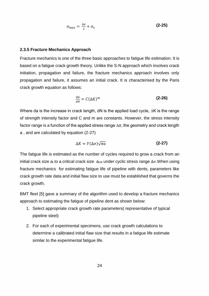
24

𝜎𝑚𝑎𝑥 = ∆𝜎

2+ 𝜎𝑜 (2-25)

2.3.5 Fracture Mechanics Approach

Fracture mechanics is one of the three basic approaches to fatigue life estimation. It is

based on a fatigue crack growth theory. Unlike the S-N approach which involves crack

initiation, propagation and failure, the fracture mechanics approach involves only

propagation and failure, it assumes an initial crack. It is characterised by the Paris

crack growth equation as follows:

𝑑𝑎

𝑑𝑁= 𝐶(∆𝐾)𝑚 (2-26)

Where da is the increase in crack length, dN is the applied load cycle, ∆K is the range

of strength intensity factor and C and m are constants. However, the stress intensity

factor range is a function of the applied stress range ∆σ, the geometry and crack length

a , and are calculated by equation (2-27)

∆𝐾 = 𝑌(∆𝜎)√𝜋𝑎 (2-27)

The fatigue life is estimated as the number of cycles required to grow a crack from an

initial crack size ai to a critical crack size acrit under cyclic stress range ∆𝜎.When using

fracture mechanics for estimating fatigue life of pipeline with dents, parameters like

crack growth rate data and initial flaw size to use must be established that governs the

crack growth.

BMT fleet [5] gave a summary of the algorithm used to develop a fracture mechanics

approach to estimating the fatigue of pipeline dent as shown below:

1. Select appropriate crack growth rate parameters( representative of typical

pipeline steel)

2. For each of experimental specimens, use crack growth calculations to

determine a calibrated initial flaw size that results in a fatigue life estimate

similar to the experimental fatigue life.

25

3. Based on the results of steps 2, develop a single initial flaw size that is

suitably representative of the experimental data

4. Calculate the fatigue lives of all the experimental specimen using the initial

flaw size determined in step 3 and the material properties selected in step 1.

2.3.6 Factors affecting fatigue life assessment of dents

There are many factors that affect the accurate prediction of fatigue life of pipeline with

a dent. From past research, it is seen that plain dents do not significantly affect the

burst strength of pipelines. However, the fatigue life reduces with increase in the dent

depth. Dent depth is one of the dent geometric properties that affect the fatigue life

estimation of dents. Other properties, such as pipe material properties, pipe geometric

properties, restraint conditions, could be also strongly correlated to the fatigue life of

dents. They are discussed as follows.

2.3.6.1 Dent geometry factor

As discussed as above, the dent depth plays a very important role in the fatigue life

estimation of dents, however, research also indicates that the dent geometry, dent

restraint and rerounding stiffness also play an important role in the fatigue estimation

of dents. Beller et al[34] in a study found that the point of maximum stress

concentration for a semi-spherical dent was at the rim of the dent. They pointed out

that as the dent was elongated, the maximum stress moved to the root of the dent.

This observation indicates that there is a critical ratio of length to width where the

location of fatigue cracking would move from the rim to the centre of the dent.

Rosenfeld[30] also concluded in a study that the ability of a dent to reround is related

to the depth to width ratio. It found out that the fatigue life also increases with increase

in depth to width d/W ratio. The width of the dent, however, was reported to be difficult

to measure due to bulging around the shoulders of the dents and is there the distance

between the points on the dents where the depth is half the maximum depth. Rinehart

and keating[35] also developed a geometric expression which is inversely proportional

to the fatigue life by combining dent depth (d/D), dent length (L/D) and rerounding

stiffness. The equation is given below.

26

𝑓𝑎𝑡𝑖𝑔𝑢𝑒 𝑙𝑖𝑓𝑒 ∝ 1

𝐿𝑑𝑊

𝐷2𝑡

(2-28)

2.3.6.2 Dent Constraint factor

Dent constraint plays a very important role in the fatigue life assessment of dents. The

ability of a dent to spring back or reround depends on whether or not there is a

constraint. Fatigue assessment comes into play when cyclic pressure is applied to the

dent. An unconstrained dent spring back upon removal of the indenter and rerounds

as pressure is applied. From research, it is seen that the fatigue life of restrained dents

is higher than equivalent unrestrained dents because of its ability to stop the dent from

rerounding due to pressure loading. Experimental work by Alexander and Kiefner [17],

keating and hoffman[36] and SES[25] have confirmed this. These tests also show that

the mode of failure in both cases are different. The tests conducted by Alexander and

Kiefner show that cracking was oriented in the circumferential direction beyond the

indenter for a restrained dent. However, in an unrestrained dent, the cracking was

axially oriented located within the dented region. Figure 2-6 below shows a comparison

between the fatigue life of unrestrained and restrained dent.

Figure 2-6 Fatigue life of unrestrained and restrained dents[1]

27

2.3.6.3 Pipe geometry factor

Pipe geometry is also an important factor that affects the fatigue life of dents in the

pipeline. Research have shown that D/t ratio affect the fatigue life of pipes. De Carvalho

Pinhiero et al[37] shows that the D/t ratio is directly proportional to the stress

concentration factor and inversely proportional to the fatigue life. However, there is a

counter claim by Dinovitzer et al [38] that showed using FEA model that the fatigue life

of dents increases with increasing D/t ratio. Fowler et al [105] undertook finite element

analysis to determine the importance of dent features. The results were used to

calculate the stress concentration factor (SCF), which was then used to calculate the

fatigue life of dented pipe. The SCF varied from 3 to 5 with different D/t ratios. Results

indicated that D/t ratio had little role to play in failure beyond a D/t of 40. FE analysis

also shows that the SCF increased rapidly from a D/t ratio of 20. It showed that the

SCF is at its peak at D/t of 50.

2.3.6.4 Pipe material factor

The pipe material property also affects the fatigue behaviour of dented pipe. Different

pipe grades are used in the pipeline industry ranging from X42 to X120. Research

confirms that fatigue life of a dented pipe decreases with increasing SMYS. Numerical

Work by Rosenfeld[30] and Dinovitzer[38] confirm this. This could be attributed to the

fact that dents can reround due to decreasing plasticity of the material.

2.3.6.5 Effect of pressure cycle

Pipeline pressure cycling plays an important role in the estimation of fatigue of pipeline

with dents. Liquid and gas pipeline can experience pressure cycling throughout the

year. For example, demand for gas is increased in winter compared to summer thereby

necessitating change in pressure. Generally, the fatigue life of pipeline with dents

decreases with increase in pressure cycling. Work by Kiefner[39] and Rosenfeld[30]

have confirmed this. The liquid pipeline tends to be more pressure cycled than the gas

pipeline as it can experience up to 1800 times the pressure cycling at the same

pressure of an equivalent gas pipeline. Kiefner[39] characterised typical pressure

cycling regime for a pipeline based on the benchmarking scheme as seen in table 2.2.

This is based on observed pressure pattern that failed as a result of fatigue. The

percentage SMYS in the table represent the hoop stress cycle. As an example, a very

28

aggressively cycled pipeline may experience 20 cycles from 72%SMYS to zero and

back to 72%SMYS

Percent

SMYS

Very

Aggressive

Aggressive Moderate Light

72 20 4 1 0

65 40 8 2 0

55 100 25 10 0

45 500 125 50 25

35 1000 250 100 50

25 2000 500 200 100

Total 3660 912 363 175

Table 2-3 benchmarked annual cycle count [39]

2.3.7 Dent measurement

Dent can be measured and detected in many ways. It can be measured by direct visual

inspection and by using various In-line inspection (ILI) tools which include magnetic

flux leakage tool, ultrasonic inspection tool and geometry tools. When measuring

dents, certain information like dent depth and shape is required and it’s associated with

weld, gouges and corrosion. Most of the ILI tools cannot measure all these information

at once and might require a combination of two or more ILI tools. Table 2-3 summarises

the capabilities of ILI tools for providing required dent information

Dent attribute Geometr

y tool

High-

resolution

geometry tool

Metal

loss tool

Crack

detection tool

29

Location along pipeline

Orientation

Size(%OD)

Size and shape of dents

Detects dents on welds

Detects metal loss in

dents

Detects cracks in dents

Detect rock dents

Table 2-4 capabilities of in-line inspection tools for dent information culled from API

1156 [18]

2.4 Finite element methodology

Finite element method (FEA) sometimes called finite element analysis (FEA) is a

numerical method for solving simple and complex engineering problems. It involves

breaking down structures into smaller (finite) elements. The equations associated with

these finite elements are then assembled into a larger system of equations that models

the entire problem. One of the common methods of dent assessment is using finite

element analysis. It can be used in place of theoretical and experimental methods. In

the past, values for peak stress, strains and SCF have been generated empirically but

nowadays, these values can be generated using finite element method. There are

various steps and techniques to follow when using finite element. These steps are

categorised into 3 groups such as pre-processing, solution and post processing. There

are several FE software packages such as Ansys, Abaqus, Nastran , Patran and so

on. Though the software interfaces are different, they all follow the same procedure in

solving problems.

30

2.4.1 Previous work done using finite element analysis

Various researchers have used finite element method. The results are validated

against experimental data. They check if it is in reasonable agreement with the

experimental data.

Leis et al [60] investigated dent on a pressurised pipe with a quarter symmetry model

using 8-node shell elements with a very refined mesh in the region of contact . The

indenter and the pipe support were modelled as rigid bodies. The results obtained from

the analysis were in reasonable agreement with the experiment data.

Ong et al [8] also studied the effect of a dent on pressurised pipeline using

experimental measurement and finite element analysis considering the effect on a

plain dent and plain dent with a reduction in wall thickness. The finite element model

consisted of quarter pipe symmetry and utilised eight node shell elements. Results

from burst test showed that pipe failure was insensitive to the existence of a local dent;

however pipe failure was found to be due to loss of thickness defect.

Zarea et al [15] proposed the use of static and dynamic FE models to estimate the

residual life of indented damaged pipes. This was done using thin triangular shell

elements for the static analysis and quadrilateral shell elements for the dynamic

analysis. They established the relationship between the depth and force, dent depth

and residual dent depth and calculated the residual stress under cyclic pressure

loading. The residual stress was then used to calculate the residual life.

Brooker [16] used a technique similar to leis et al to model denting of pressurised

pipeline under localised radial loading. The model included an 8-node full integration

solid elements in the dent region with five layers through the wall thickness of the pipe

and 8-noded shell elements away from the dent region. Contact between the pipeline

and the indenter was modelled with the assumption that the surface was frictionless. It

was observed that the indenter shape and size was imperative to pipeline puncture.

He also observed that the puncture load can be taken as proportional to the pipe

thickness and linearly related to the material ultimate stress. Brooker [16] proposed an

equation after the numerical study for lateral indentation showing the influence of pipe

diameter and thickness, pipe length and residual depth on the indenting force.

31

BMT fleet[5] in a study compared five methodologies employed by researchers in

fatigue life assessment in order to determine what the cause of conservatism in the

approach. They came to the following conclusions

All the methods studied utilise the S-N approach which is as a result of a wide

range of S-N curves available for use

Isotropic hardening model was used by four methods to idealise the cyclic

material behaviour of the pipe

The stress concentration factor for all the methods was calculated as a function

the dent depth (d/D) and the pipe geometry(D/t). Three of the methods

accounted for the effect of mean pressure

Two of the methods accounted for the dent shape

2.5 Artificial neural network

The term neural network derived its origin from the human brain or the human nervous

system which consist of a large parallel interconnection of a large number of neurones.

The human brain has a highly complex non-linear parallel computer and can organise

its structural constituents known as neurones. Neurones interact with each other

through a host of structures called dentrites[49]. These neurones are interconnected

in a very complex way between each other to create a network. The artificial neural

network mimics a small part of the human brain to perform some specific task such as

data classification or pattern recognition through a learning process. It has an inter-

connection of non-linear neurones that are distributed throughout. When using it for

non-numeric values, It is called classification. However using it for numerical values is

called regression.

An artificial neural network consists of a set of neurons or processing element (PE)

that are connected by links of certain numeric weights. Each neuron has

a set of input links from other neurons

a set of output links from other neurons

a current activation function

32

and an activation function to compute the activation level in the next time step

A typical neuron is illustrated in figure 2-7

Figure 2-7 A typical neuron in a neural network [50]

In figure 2-12, x1, x2…xn are the inputs, w1j, w2j….wnj are the weights. The total

weighted input is the sum of the input activation multiplied by their respective weights

Neural networks have the capacity to derive meaning from loose information, can be

utilized to detect trends and identify patterns that are too intricate to ever be seen by

either people or other PC procedures. A trained neural network can be considered as

a "specialist" in the class of data it has been given to examine.

Other advantages include:

1. Adaptive learning: A capacity to figure out how to do assignments in view of the

information given for training

2. Self-Organization: An ANN can make its own particular association or representation

of the data it gets amid learning time.

33

3. Ongoing Operation: ANN calculations might be completed in parallel, and

exceptional equipment gadgets are being designed and fabricated which exploit this

capacity.

2.5.1 Neural network architecture

A typical neural network architecture will consist of an input layer, one or more hidden

layer, and an output layer. The input layer represents the information that is being fed

into the system. The hidden layer is dictated by the activities of the input units and the

weights between the input and hidden layer. The output layer likewise relies on the

action of the hidden layer and weights between the input and output layer

The architecture can be further categorised into

single layer architecture

multiple layer architectures

The single-layer association, in which all units are associated with each other,

constitutes the broadest case and is of more potential computational force than

progressively organized multi-layer associations. In multi-layer systems, units are

regularly numbered by layer, rather than taking after a global numbering.

2.5.1.1 Feedforward network

A feed forward network which is shown in figure 2-8 permits signal in one direction only

(i.e. from input to output).There is no form of feedback within the system and is usually

used in pattern recognition

Figure 2-8 A feed forward network [51]

34

The typical characteristic of a feed forward system include:

1 .perceptron are arranged in layers, the input being the first layer and the output being

the last layer. In-between the input and the output layer, there is a hidden layer that

has no connection with the external world

2. Each perceptron within one layer is connected to every perceptron in the next layer

and information is constantly fed forward from one layer to the next

3 perceptrons within a layer are not connected in any way

The number of neurons in the input layer is equal to the number of input variables,

similarly, the number of the output layer is equal to the number of output variables. The

accuracy of the model is determined by the number of neurons in the hidden layer.

There are several algorithms that can be used to train a neural network. Some of them

include back-propagation, genetic algorithm, and particle swam optimisation. For this

study, the back propagation algorithm is used as it is the fastest and the most common

technique. It also gives insight on how the weights and biases can affect the behaviour

of the network

2.5.2 Activation functions

The behaviour of an ANN greatly depends on the activation function, weights, and

biases. There are different types of activation functions. The most common ones are

the logistic sigmoid and the hyperbolic tangent transfer functions. Both functions are

compared to determine the one that best predicts the SCF. Neural network learning

One of the unique characteristics of an artificial neural network is its ability to learn and

recognise pattern. ANN models its learning process by adjusting the weighted

connections between neurons in a network. There are several learning algorithms that

can be used when training an artificial neural network. The objective of the learning

algorithm is to find a set of weight matrices which if applied to the network would map

any input to a correct output

35

2.5.2.1 Supervised learning

This is the type of learning algorithm that provides the desired output and input while

training the network. An error can be calculated based on the target output and actual

output by providing the network with a pair of input and output. Through the errors, the

network can make corrections by adjusting the weight matrix. There are several

supervised learning algorithms and the most common are the back-propagation

algorithm

2.5.2.2 Backpropagation

The back-propagation algorithm computes each error derivative of the weights (EW)

by first computing the rate at which the error change as the activity level of a unit is

changed (EA).For the output, The EA is the difference between the actual and the

desired output. The EA of the hidden unit is calculated by first identifying all the weights

between the hidden units and the output units to which it is connected. The weights

are then multiplied by the EAs of the output units, the products are then added. The

sum equal the EA for the chosen hidden unit. The EAs for other layers are calculated

in similar fashion moving from layer to layer in a direction opposite the way activities

propagate through the network. The EW is the product of the EA and the activity

through the incoming connection [49]

2.5.2.3 Unsupervised learning

The learning algorithm for an unsupervised learning involves feeding the network with

given set of inputs. The neural network then finds a pattern within the input provided

without no external aid to create an output.

36

CHAPTER 3

ELASTIC SPRING BACK AND REROUNDING IN DENTED

PIPELINE

3.1 Introduction

This chapter focuses on the response of the pipe during the denting and the

pressurisation process. The pipe’s response to denting is dependent on some key

parameters. These parameters include pipe geometry, dent geometry, pipe material

and applied pressure range. When a pipe is dented, the elastic response of the pipe is

dependent on these variables. Steel pipes have both elastic and plastic properties.

When a pipe is dented, the elastic property comes into effect allowing some spring

back in the dents when the cause of denting is released. However, the pipe does not

fully gain its original position leaving some plastic deformation. Upon application of

pressure, the dent depth is reduced further but does not fully regain its original position.

In most experimental data, dent depths are measured after spring back at zero

operating pressure and this represents the scenario when a dent is formed during

construction. However, in practice dents are introduced in service under internal

pressure and the dent depth measured are the rerounding dent depths . The responses

of the pipe to the denting process are different and the stress level associated with

these scenarios are also different. This led to the introduction of spring back correction

factor and triggered the debate about which dent depth should be used in assessment.

Cosham and Hopkins have reviewed a number of correction factors and have come to

the conclusion that most spring back correction factors are empirically derived and do

not account for some parameters including, pipe geometry, dent geometry, and pipe

materials. Available test data have a lot of scatters in relation to the rerounding, making

the prediction increasingly difficult.

The objectives of this chapter is to

improve the understanding of the spring-back and re-rounding phenomenon

Identify the most important parameters, which influences spring-back and re-

rounding

37

create database for the application of ANN-based formulae in chapter 6

provide guidance in how to apply the additional knowledge

3.2 Spring back and rerounding mechanism

The process of denting produces both elastic and plastic responses in the material.

When an indenter is applied to the pipe to create dent and removed, the elastic

component of the deformation is recovered and the dent will naturally move outwards

reducing the dent depth. This recovery is referred to as ‘spring back’. At this point the

dent does not fully move out, leaving some plastic deformation. When internal pressure

is introduced to the pipe, the dent further pushes out. This phenomenon is called

‘rerounding’. The extent to which the dent is pushed out is dependent on the magnitude

of internal pressure. As the internal pressure is increased, the dent is further pushed

out which consequently reduces the dent depth. Rosenfeld[11] postulated that the

process of rerounding includes an initial plastic recovery of the dent depth which is

dependent on the pipe properties and internal pressure. Whether further rerounding is

plastic or elastic is determined by the magnitude of the stress cycles. It postulates that

the dent will eventually shakedown to stable elastic behaviour when the dent depth

cycles about a mean depth, which is a function of the geometry and the amplitude of

the pressure fluctuations.

3.3 Finite element model

The finite element model is a critical part of this research. The results obtained from

this study is used to train the artificial neural network (ANN). It is essential to get an

accurate result from this study and the accuracy is dependent on the model itself. BMT

fleet[5] compared some methodologies as discussed in chapter 2 and suggested some

factors that might be the cause of conservatism in FE results. Included in these factors

are the material model used in characterising the cyclic behaviour of the model and

the type of analysis itself. This section carefully studies these factors and how it can

affect the results in general. There are several steps involved in the modelling such as

material assignment, geometry creation, meshing, contact pair creation, boundary

conditions and loading. Each of these steps needs to be done correctly in order to

obtain an accurate result. In order to create a wider range of data, a total of 256 models

are created. These models have varying diameter to thickness ratio (D/t), dent

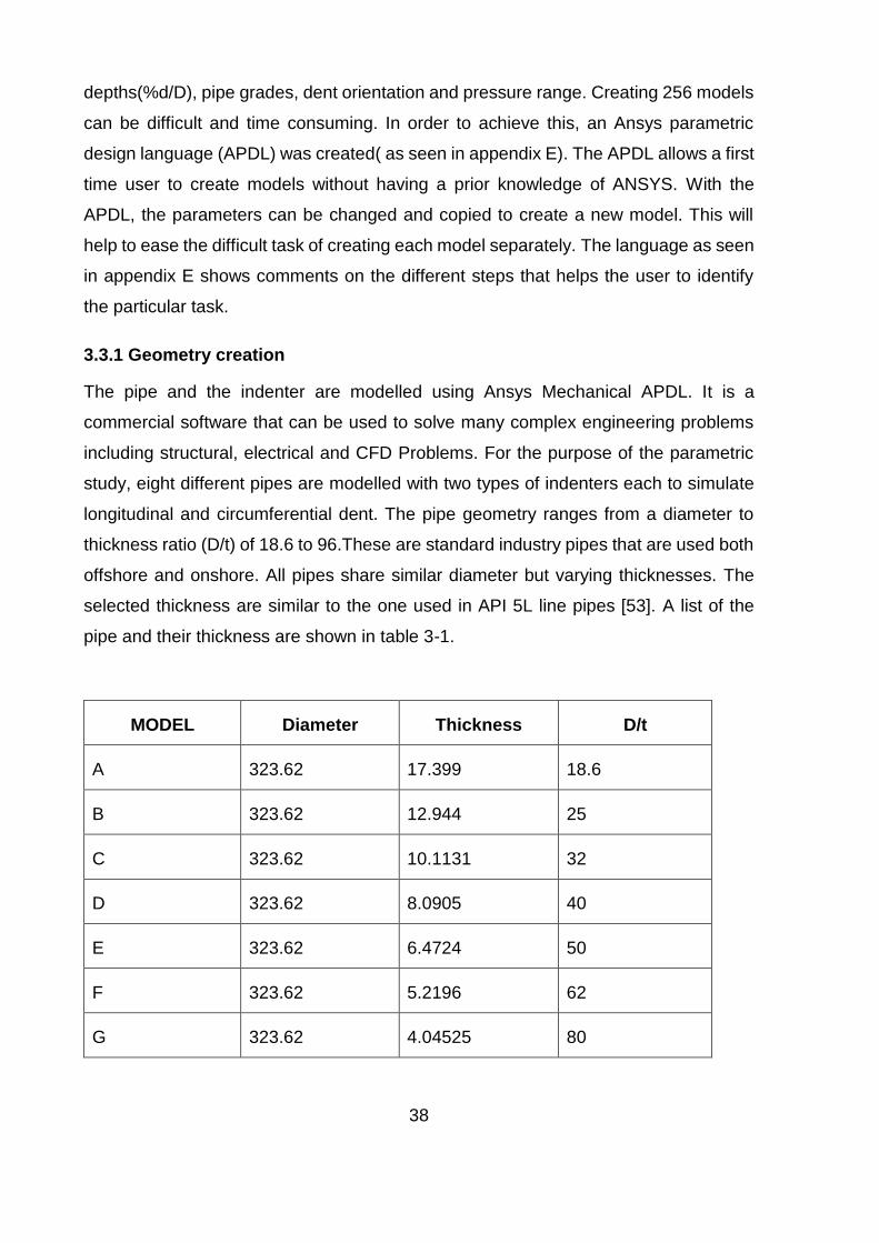
38

depths(%d/D), pipe grades, dent orientation and pressure range. Creating 256 models

can be difficult and time consuming. In order to achieve this, an Ansys parametric

design language (APDL) was created( as seen in appendix E). The APDL allows a first

time user to create models without having a prior knowledge of ANSYS. With the

APDL, the parameters can be changed and copied to create a new model. This will

help to ease the difficult task of creating each model separately. The language as seen

in appendix E shows comments on the different steps that helps the user to identify

the particular task.

3.3.1 Geometry creation

The pipe and the indenter are modelled using Ansys Mechanical APDL. It is a

commercial software that can be used to solve many complex engineering problems

including structural, electrical and CFD Problems. For the purpose of the parametric

study, eight different pipes are modelled with two types of indenters each to simulate

longitudinal and circumferential dent. The pipe geometry ranges from a diameter to

thickness ratio (D/t) of 18.6 to 96.These are standard industry pipes that are used both

offshore and onshore. All pipes share similar diameter but varying thicknesses. The

selected thickness are similar to the one used in API 5L line pipes [53]. A list of the

pipe and their thickness are shown in table 3-1.

MODEL Diameter Thickness D/t

A 323.62 17.399 18.6

B 323.62 12.944 25

C 323.62 10.1131 32

D 323.62 8.0905 40

E 323.62 6.4724 50

F 323.62 5.2196 62

G 323.62 4.04525 80

39

H 323.62 3.371 96

Table 3-1 pipe models and dimensions

The indenter used includes a longitudinal bar indenter with dimensions 609.6mm x

304.5mm x 50.8mm and a dome indenter with diameter 219.07mm. The shapes and

sizes of these indenters were selected in order to vary the sizes (particularly the length

of the dent) and the dent orientation and to ultimately see their effects on the result.

A Quarter model of both the pipe and the indenter are modelled taking advantage of

the symmetry of the pipes and indenters. A sufficient length of pipe is used to avoid

interaction with the boundaries. Figure 3-1 shows the model for a longitudinal and

circumferential dent.

(a)

40

(b)

Figure 3-1 Longitudinal (a) and circumferential (b) dent models

The entire model has two major volumes which consist of the quarter symmetry of the

pipe and quarter symmetry of the indenter. The pipe is further divided into 3 regions as

seen in the figure above. The advantage of this is that it helps to easily mesh the model

and the region of interest can be easily separated from the entire model. Region 1

represents the region of interest as this is the region where the high-stress

concentration takes place. It also represents the region of high mesh density. Region

2 is the transition region. It represents the region where the mesh transitions from a

higher density to a lower density. The third region represented as 3 is the region of

lower mesh density.

3.3.2 Materials

Four different pipes grades are considered in the parametric study. They include X46,

X65, X80, and X100. The response of the material to denting depends majorly on the

material model so it is important to get the material modelling right. For this study, a

multi-linear kinematic model is used to adequately simulate the response of the

material during denting, rerounding and pressure cycling. This model is a rate

independent version of the kinematic hardening model and is very useful in modelling

cyclic plastic behaviour. It assumes that yield surface remains constant in size but

41

allows translation due to plasticity. It also accounts for the Baushinger effect in that

material's stress/strain characteristics change as a result of the microscopic stress

distribution of the material. The stress-strain curve for each of the materials is seen in

figure 3-2, 3-3, 3-4 and 3-5. Table 3-2 also shows the mechanical properties of each

material model. Each material has a young’s modulus of 210000Mpa and a Poisson’s

ratio of 0.3.

Figure 3-2 Stress-strain curve for X46


0

50

100

150

200

250

300

350

400

450

500

0 0.02 0.04 0.06 0.08 0.1 0.12 0.14 0.16

Stre

ss(

Mp

a)

Strain

X46

0

100

200

300

400

500

600

700

800

900

1000

-0.2 0 0.2 0.4 0.6 0.8 1 1.2

Stre

ss (

Mp

a)

Strain

X65

42



0

100

200

300

400

500

600

700

0 0.01 0.02 0.03 0.04 0.05 0.06 0.07

Stre

ss (

Mp

a)

Strain

X80

0

100

200

300

400

500

600

700

800

900

0 0.01 0.02 0.03 0.04 0.05 0.06

Stre

ss (

Mp

a)

Strain

X100

43

API 5L grade Yield strength

(Mpa)

Ultimate

tensile

strength (Mpa)

X46 317 434

X65 448 530

X80 551 620

X100 690 760

Table 3-2 mechanical properties of pipe models

3.3.3 Elements

It is essential to choose the right element type for the model as it determines the

behaviour of the model and its responses to external loads. A solid 186 element is

used to model both the pipe and indenter. Contact and target elements CONTA 174

and TARGE 170 are used in modelling the contact pair.

3.3.3.1 Solid 186

The solid186 is a higher order 3D 20 node solid element having three degrees of

freedom per node that exhibits quadratic displacement behaviour. This element

supports hyper-elasticity, plasticity, large deflection, stress stiffening and large strain

capabilities. It can also be used for modelling deformations of nearly incompressible

elastoplastic materials and fully incompressible hyperelastic materials. The solid 186

elements are usually available in two forms which include

The homogeneous structural solid

Layered structural solid

The homogenous structural solid is usually useful for modelling irregular meshes while

the layered structural solid is usually used to model layered thick shells or solid a typical

diagram of a homogeneous and a layered structural solid element is given in figures

3-6 and 3-7.

44

Figure 3-6 Homogeneous structural solid element[52]

Figure 3-7 Layered structural solid elements[52]

45

For this study, the homogeneous structural solid element is used. Pressures may be

input as surface loads on the element faces as shown by the circled numbers on figure

3-6 above. Positive pressure acts on the elements.

3.3.3.2 Conta 174

This element can be applied to a 3D structural contact analysis and is used to represent

contact and sliding between 3D target surfaces and the deformable surface defined by

this element. It can be used as either a pair based contact or general contact. In the

case of a pair based contact which is used in this study, the target surface is

determined by the 3D target element TARGE170.The element is found on the surfaces

of the solid element with mid-side nodes such as SOLID186 used in this study. It has

the same geometric characteristics as the SOLID186 element face with which it is

connected. A typical diagram of a CONTA174 element is shown in figure 3-8.

Figure 3-8 Conta174 element

3.3.3.3 Targe170

The targe170 element is usually combined with a contact element. In this study, it is

combined with the Conta174 element. It is used to represent the various 3-D target

surface for the associated contact element. Target surfaces can either be rigid or

flexible. Rigid surface must be represented by a target surface for a rigid-flexible

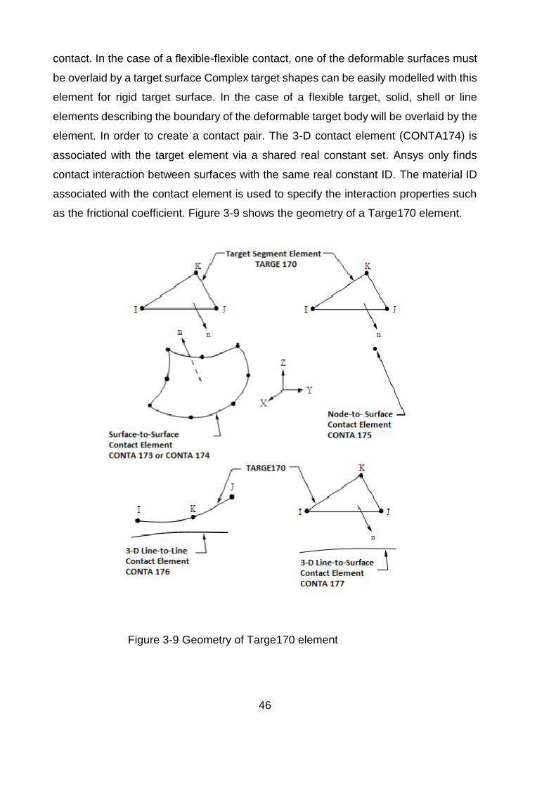
46

contact. In the case of a flexible-flexible contact, one of the deformable surfaces must

be overlaid by a target surface Complex target shapes can be easily modelled with this

element for rigid target surface. In the case of a flexible target, solid, shell or line

elements describing the boundary of the deformable target body will be overlaid by the

element. In order to create a contact pair. The 3-D contact element (CONTA174) is

associated with the target element via a shared real constant set. Ansys only finds

contact interaction between surfaces with the same real constant ID. The material ID

associated with the contact element is used to specify the interaction properties such

as the frictional coefficient. Figure 3-9 shows the geometry of a Targe170 element.

Figure 3-9 Geometry of Targe170 element

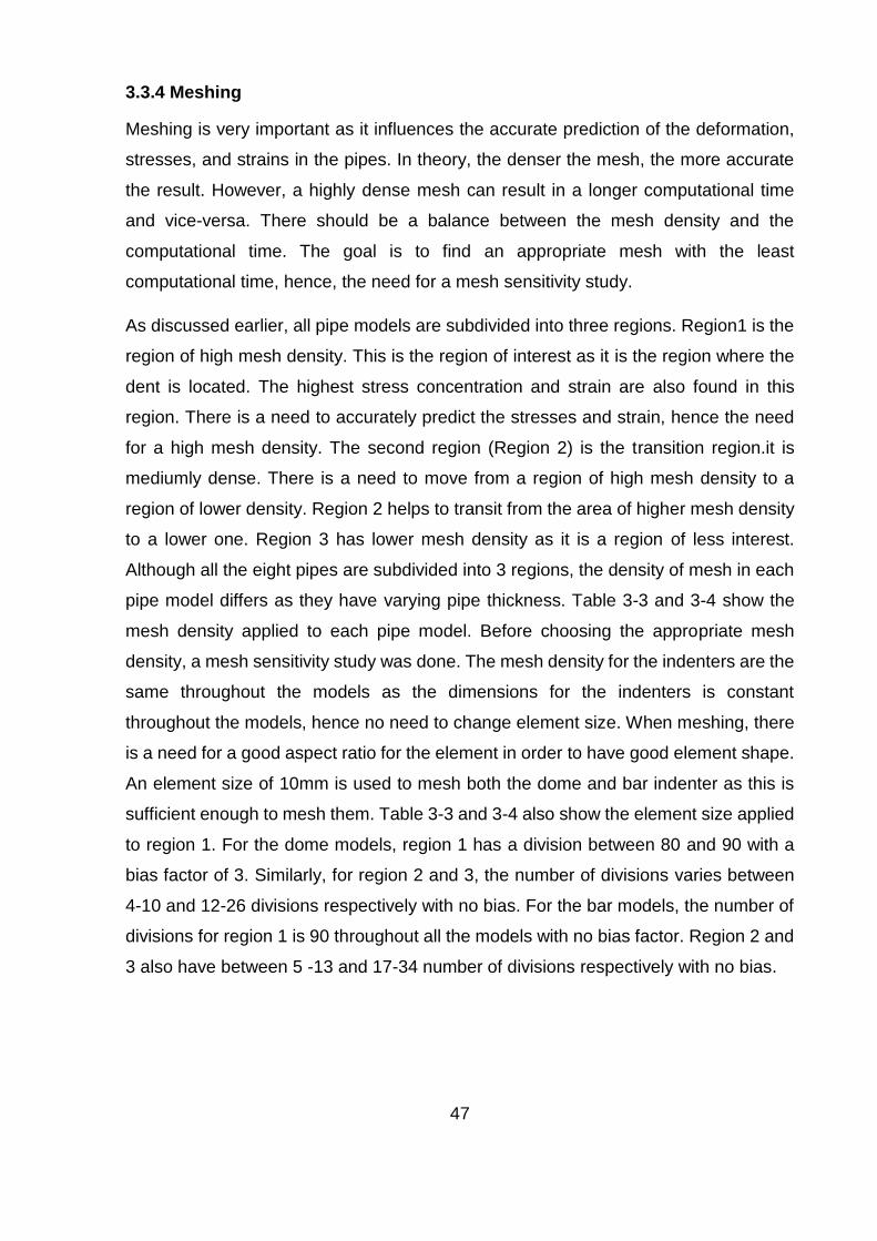
47

3.3.4 Meshing

Meshing is very important as it influences the accurate prediction of the deformation,

stresses, and strains in the pipes. In theory, the denser the mesh, the more accurate

the result. However, a highly dense mesh can result in a longer computational time

and vice-versa. There should be a balance between the mesh density and the

computational time. The goal is to find an appropriate mesh with the least

computational time, hence, the need for a mesh sensitivity study.

As discussed earlier, all pipe models are subdivided into three regions. Region1 is the

region of high mesh density. This is the region of interest as it is the region where the

dent is located. The highest stress concentration and strain are also found in this

region. There is a need to accurately predict the stresses and strain, hence the need

for a high mesh density. The second region (Region 2) is the transition region.it is

mediumly dense. There is a need to move from a region of high mesh density to a

region of lower density. Region 2 helps to transit from the area of higher mesh density

to a lower one. Region 3 has lower mesh density as it is a region of less interest.

Although all the eight pipes are subdivided into 3 regions, the density of mesh in each

pipe model differs as they have varying pipe thickness. Table 3-3 and 3-4 show the

mesh density applied to each pipe model. Before choosing the appropriate mesh

density, a mesh sensitivity study was done. The mesh density for the indenters are the

same throughout the models as the dimensions for the indenters is constant

throughout the models, hence no need to change element size. When meshing, there

is a need for a good aspect ratio for the element in order to have good element shape.

An element size of 10mm is used to mesh both the dome and bar indenter as this is

sufficient enough to mesh them. Table 3-3 and 3-4 also show the element size applied

to region 1. For the dome models, region 1 has a division between 80 and 90 with a

bias factor of 3. Similarly, for region 2 and 3, the number of divisions varies between

4-10 and 12-26 divisions respectively with no bias. For the bar models, the number of

divisions for region 1 is 90 throughout all the models with no bias factor. Region 2 and

3 also have between 5 -13 and 17-34 number of divisions respectively with no bias.

48

Model Thickness

(mm)

No of

division

across

thickness

No of

divisions

across

region1

Element

size at

region

1(mm)

No of

divisions

across

region 2

No of

divisions

across

region 3

No of

divisions

across

half

circumfer

ence

Total

number of

elements

A 17.399 6 80 3 4 12 50 32016

B 12.944 6 90 2.5 5 17 50 36216

C 10.1131 4 80 3 5 17 50 23316

D 8.0905 4 80 2.5 5 18 50 23516

E 6.4724 3 80 3 5 17 50 18216

F 5.2196 3 80 2.5 6 21 50 18966

G 4.0452 3 80 2 10 27 50 20466

H 3.371 2 80 2 9 26 50 14616

Table 3-3 Meshing for dome models

Model Thickness

(mm)

No of

division

across

thickness

No of

divisions

across

region1

Element

size at

region 1

No of

divisions

across

region 2

No of

divisions

across

region 3

No of

divisions

across half

circumference

Total

number

of

elements

A 17.399 6 90 3 5 17 50 35346

B 12.944 6 90 2.5 5 17 50 35346

C 10.1131 5 90 2.5 6 18 50 30296

D 8.0905 4 90 2.5 6 17 50 24446

E 6.4724 3 90 3 5 17 50 18696

F 5.2196 3 90 2.5 7 20 50 19446

G 4.0452 3 90 2 8 29 50 20946

H 3.371 3 90 1.5 13 34 50 22446

49

Table 3-4 meshing for bar models

(a)

(b)

Figure 3-10 Mesh models for Dome (a) and Bar (b) indenters

50

3.3.5 Boundary conditions

Getting the boundary conditions right is very important as it affects the calculated

result. The boundary conditions are set in a way that it represents how they are

constrained and loaded in a real life scenario. The model is constrained on both the

side and bottom of the pipe. A remote displacement is applied on the end face of the

pipe as indicated by the green arrow in figure 3-11. Here, the X and Y components are

free and the Z component is set at zero. This allows the pipe to expand in radial

direction when pressurised. Similarly, remote displacement is applied to the bottom

line of the pipe, The X and Z components are free but the Y component is set at zero

in order not to allow movement in the Y direction during the denting process.

As discussed earlier, a quarter pipe and indenter are modelled considering the

symmetry of the pipe and indenter to reduce the computation time. Symmetry

boundary condition is put on the sectional faces of the pipe as shown in figure 3-12.

The symmetry boundary constraint mirrors all loading and boundary conditions from

the quarter pipe to the other parts of the pipe.

Figure 3-11 Model constraint

51

Figure 3-12 Symmetry boundary condition

3.3.6 Contact pair creation

In order to simulate the denting process, a contact pair is created between the

indenters and outer pipe surface. Before creation, contact and target nodes are created

from the indenter and pipe. The models represent a rigid-flexible contact, therefore the

indenter surface represents the target surface and target nodes are shown in Figure

3-13a. Figure 3-13b represents the contact nodes and the contact pair is shown in

figure 3-14. The properties of the contact pair include a frictional surface with a

coefficient of friction of 0.2, reduced penetration and a symmetric stiffness matrix.

52

Figure 3-13 Contact and target nodes

Figure 3-14 Contact pair

3.3.7 Loading

The loading sequence is similar to that of experimental procedures. The aim is to

measure the spring back and reround depth after indentation and pressurisation

respectively. The model involves several load steps. The first load step is the

indentation process, the second load step is the removal of the indenter to allow spring

back. Other load steps include pressurising the pipe up to 72%SMYS which is the

maximum allowable operating pressure (MAOP). The last load step involves removing

the internal pressure to measure the reround depth.

The pipe has both elastic and plastic properties and as a result, a displacement greater

than the expected dent depth is applied on the indenter. This is so because, after

indentation, the elastic portion of the pipe comes into effect by trying to regain its

original position leaving a plastic deformation. This effect is called spring back. The

indentation process is done at zero applied pressure which represents construction

dents. Figure 3-15 shows a graphical representation of the indentation process (a) and

the indenter removal (b)

After the removal of the indenter, an initial pressure of up to 80%MAOP is applied to

the inner pipe wall.10 cycles of pressure ranging from 10% to72% SMYS is the then

applied afterwards. Finally, the pressure is removed to measure the residual dent

depth.

53

(a) (b)

Figure 3-15 Denting process (a) and indenter removal (b)

3.4 Spring back results

The result from this study has indicated that spring back of the pipe is dependent on

some parameters. These parameters can be seen to greatly influence the elastic

spring back of the dent. These parameters include pipe geometry, dent geometry, and

the material strength.

3.4.1 Effect of pipe geometry on spring back

The graph below shows the effect of pipe geometry on the spring back of dents for an

X46 pipe grade. The ratio of the initial depth Hi to the spring back depth Ho(measured

depth) is plotted against the different diameter to thickness ratios of the pipes of the

same dent depth category. This is done for all the dent depth categories i.e. 2% to

10%. From the graph, it is seen that the ratio of the initial dent depth(Hi) to the spring

back depth(Ho) increases as D/t increases. This was also done with other pipe grades

and the results are indicating similar trend. The results clearly shows that the diameter

to thickness ratio of the pipe is critical in determining the spring back depth of the pipe

54

(a)

(b)

Figure 3-16 effects of pipe geometry on spring back for a dome (a) and bar (b) X46

pipe grade

3.4.2 Effect of dent geometry on spring back

Figure 3-17 shows the effect of dent geometry on the spring back of the dent. An X100

pipe grade is chosen to illustrate the results. The ratio of the initial dent depth Hi to the

spring back depth Ho is plotted against the diameter to thickness ratio (D/t). The two

dent types (dome and bar) are compared for the four dent depth categories. From the

graph, it is clearly seen that the ratio of the initial to measured dent depths (Hi/Ho) is

higher for a bar indenter compared to a dome indenter for the same dent category.

0.0

0.5

1.0

1.5

2.0

2.5

0 20 40 60 80 100 120

Hi/H

o

D/t

X46

2%

5%

7%

10%

0.0

1.0

2.0

3.0

4.0

5.0

0 20 40 60 80 100 120

Hi/H

o

D/t

X46

2%

5%

7%

10%

55

This shows that elastic recovery is higher in shorter dent lengths than the longer dent

length. Results also show that the ratio decreases as the dent depth increase. As the

dent depths increases further, the ratio of the initial to the measured depths becomes

more stable. However smaller dent depths (2% d/D) exhibits the highest ratio. This

equally shows that the elastic recovery in pipeline dents is higher in deeper dents

compared to shallow dents. The same result was reflected on all of the other pipe

grades as seen in appendix A2.

Figure 3-17 effects of dent geometry on spring back for an X100 pipe grade

3.4.3 Effect of pipe grade on spring back

Figure 3-18 illustrates the effect of pipe grade on the spring back of dent for a 10% d/D

for both dome and bar models for the four different pipe grades. Both graphs show that

the ratio of the initial Hi to the measured Ho increases as the pipe yield strength

increases. The lower ratios indicates less elastic recovery, hence, there is a more

elastic recovery in higher pipe grades compared to lower pipe grades . This could be

attributed to the yield strength of the pipe and the material stiffness. The result is same

for both the dome and the bar indenter. Other models are analysed with different dent

depths and the result show that they all exhibit similar behaviour as seen in appendix

A3.

0

1

2

3

4

5

6

7

8

9

10

0 20 40 60 80 100 120

Hi/H

o

D/t

2% dome

2% bar

5% dome

5% bar

7% dome

7% bar

10% dome

10% bar

56

(a)

(b)

Figure 3-18 effect of pipe material on spring back for a 10% dome(a) and bar(b)

X100 pipe grade

3.5 Result for rerounding

The above results show the responses of the pipe dent during and after indentation.

However, when the internal pressure is introduced, rerounding occurs. The dent is

further pushed out and the dent depth decreases as the pressure is increased.

0.0

0.5

1.0

1.5

2.0

2.5

0 20 40 60 80 100 120

Hi/H

o

D/t

X46

X65

X80

X100

0.0

0.5

1.0

1.5

2.0

2.5

3.0

0 20 40 60 80 100 120

Hi/H

o

D/t

10% bar

X46

X65

X80

X100

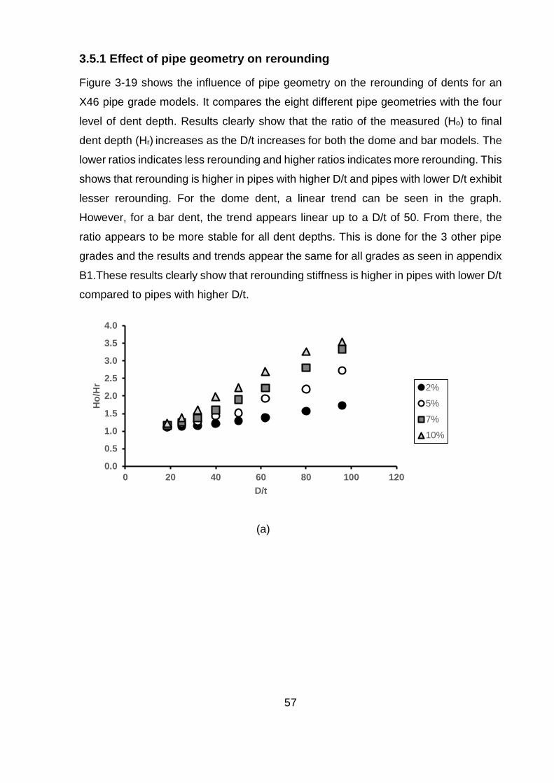
57

3.5.1 Effect of pipe geometry on rerounding

Figure 3-19 shows the influence of pipe geometry on the rerounding of dents for an

X46 pipe grade models. It compares the eight different pipe geometries with the four

level of dent depth. Results clearly show that the ratio of the measured (Ho) to final

dent depth (Hr) increases as the D/t increases for both the dome and bar models. The

lower ratios indicates less rerounding and higher ratios indicates more rerounding. This

shows that rerounding is higher in pipes with higher D/t and pipes with lower D/t exhibit

lesser rerounding. For the dome dent, a linear trend can be seen in the graph.

However, for a bar dent, the trend appears linear up to a D/t of 50. From there, the

ratio appears to be more stable for all dent depths. This is done for the 3 other pipe

grades and the results and trends appear the same for all grades as seen in appendix

B1.These results clearly show that rerounding stiffness is higher in pipes with lower D/t

compared to pipes with higher D/t.

(a)

0.0

0.5

1.0

1.5

2.0

2.5

3.0

3.5

4.0

0 20 40 60 80 100 120

Ho

/Hr

D/t

2%

5%

7%

10%

58

(b)

Figure 3-19 effect of pipe geometry on rerounding for a X46 dome (a) and bar(b) dent

3.5.2 Effect of dent geometry on rerounding

Figure 3-20 shows the result for effect of dent geometry for an X46 pipe grade. Four

dent depths are simulated for each of the dent type. This was done on all the pipe

geometries. From figure 3-20, it can be seen that the ratio of the measured to the final

dent depth Ho/Hr increases as the dent depth increases. Similarly, it can be seen that

the ratio is higher for a longitudinal type dent compared to a circumferential type dent

up to a D/t of 50, However, as the D/t increases further, the ratio becomes higher in

circumferential dent compared to the longitudinal dent. This is so because the

circumferential models show a linear pattern as opposed the longitudinal models that

exhibit a non-linear pattern. It can also be seen from the results that the margins

between the ratios of the measured to the final dent depths are closer in value for

smaller D/t. However, as the D/t increases further, the margin between the ratios of

each depth increase further.

0.0

0.5

1.0

1.5

2.0

2.5

3.0

3.5

0 20 40 60 80 100 120

Ho

/Hr

D/t

2%

5%

7%

10%

59

Figure 3-20 effects of dent geometry on rerounding for an X46 pipe grade

3.5.3 Effect of pipe material on rerounding

The result has shown that the pipe grades can influence the reround depth of dent.

Figure 3-21 illustrate the effect of pipe material on a 10% dome and an equivalent bar

dent for all the pipe grades. It can be seen from the graph that the ratio of the measured

to the final dent depth increases as the pipe grade increases for an equivalent D/t.

Results show that higher pipe grades experience more rerounding compared to a lower

pipe grade for a dome dent. However, the margin between ratios appears very close

in the bar dents, though it is clear in some cases that the higher pipe grades have a

higher ratio of the measured to final dent depths. Other dent depths (i.e. 2%, 5% and

7%) are analysed and results show similar pattern and trend as seen in appendix B3.

0.0

0.5

1.0

1.5

2.0

2.5

3.0

3.5

4.0

0 20 40 60 80 100 120

Ho

/Hr

D/t

2% dome

2% bar

5% dome

5% bar

7% dome

7% bar

10% dome

10% bar

60

(a)

(b)

Figure 3-21 effects of pipe material on rerounding for a 10% dome (a) and bar (b)

dent

0.0

0.5

1.0

1.5

2.0

2.5

3.0

3.5

4.0

4.5

5.0

0 20 40 60 80 100 120

Ho

/Hr

D/t

X46

X65

X80

X100

0.0

0.5

1.0

1.5

2.0

2.5

3.0

3.5

4.0

0 20 40 60 80 100 120

Ho

/Hr

D/t

X46

X65

X80

X100

61

3.6 Comparison of experimental and finite element model

The finite element models are validated against experiment data. The experimental

data used in this study is the experimental project sponsored by American petroleum

institute to study the effect of smooth and rock dents on liquid petroleum pipelines [17].

The experiment uses a dome and a bar indenter with pipes of varying diameter and

thicknesses. With limited data, plots of the initial dent depth (Hi) versus spring back

(Ho) depth and reround depth (Hr) are used to validate the dome model.

3.6.1 Spring back validation

Table 3-5 shows a comparison between experimental results and FEA results. The

initial dent depth Hi and spring back depth Ho for a dome indenter are compared for

the experimental and FEA result. Though the data are limited, the finite element model

gave a good correlation to the experimental model with a maximum percentage error

of 17% as seen in table 3-5

Serial

No

Experimental[17] FEA %

error Hi(mm) Ho(mm) Hi/Ho Hi(mm) Ho(mm) Hi/Ho

1 6 4.55 1.31 6.2 4 1.55 15

2 12 6.8 1.76 12.2 8 1.52 14

3 18 10.7 1.68 18.1 13 1.39 17

4 18 11.3 1.59 18.1 13.1 1.38 13

Table 3-5 comparison between experimental[17] and FEA results for spring back

3.6.2 Rerounding validation

Table 3-6 similarly shows a comparison between experimental[17] and FEA results. It

compares the initial dent depth Hi and reround Hr depth of some selected dataset of

the experimental result with FEA results. The table shows a good correlation between

the experimental model and finite element model with a maximum percentage error of

16%.

62

Serial

No

Experimental[17] FEA %

error Ho(mm) Hr(mm) Ho/Hr Ho(mm) Hr(mm) Ho/Hr

1 6 1.55 3.8 6.2 1.8 3.4 10.5

2 12 3.8 3.2 12.2 3.2 3.8 16

3 18 3 6 18.1 3 6 0

Table 3-6 comparison between experimental[17] and FEA results for rerounding

3.7 Summary of result and conclusion

The above results have shown how parameters like pipe geometry, dent geometry,

and pipe material affect the spring back response and rerounding of the pipe to denting.

These parameters are significant in predicting the spring back response and

rerounding of the dents. The various conclusions drawn from this study are as follows:

1. The pipe geometry influences both the spring back and reounding of the dent.

The ratio of the initial dent depth to the elastic spring back increases with

increasing D/t. Similarly, the ratio of the measured dent depth to final dent depth

(after pressurisation) increases with increase in the D/t

2. The dent geometry is another critical factor influencing spring back and

rerounding. The ratio of the initial dent to the measured dent is higher for longer

dents compared to shorter dents. This is an indication that elastic recovery is

higher in longer dents compared to shorter dents. However, the ratio of the

measured depth to the final depth reduces as the dent depth increases. This

clearly shows that deeper dents have less elastic recovery than shallow dents.

The ratio of the measured depth to the final depth is equally higher for longer

dents compared to short dents. On the contrary, for rerounding, the ratio of the

measured to final depths increases as the dent depth increases.

3. Pipe material also influences the spring back and rerounding, results have

shown that both the ratio of the initial to the measured depth and the ratio of the

measured depth to the final depth increases with increasing pipe grades. This

63

indicates that pipes with lesser strength exhibit less elastic spring back and

rerounding compared to pipes with higher material strength.

64

CHAPTER 4

FATIGUE ANALYSIS OF PLAIN DENTS USING SN

APPROACH

4.1 Introduction

The S-N approach is the most common approach in determining the fatigue life

of pipes with dents. The method involves using a published fatigue S-N curve from

appropriate design code and accounting for stress concentration in the dents by the

use of stress concentration factors (SCF).The cycles to failure can be determined from

the curve to determine the fatigue life. The common S-N curves used in dent

assessment today are the API RP2A curve ‘X’ [29], DOE curve B[28], DIN2413 [26]

and ASME BPVC Div 2 fatigue life curve.

Many researchers have used the S-N approach to determine the fatigue life of

dents in the pipeline. Fowler et al [25] combined experimental and numerical projects

by using the API RP2A curve ‘X’ and the DOE curve B to determine the fatigue life of

dented pipelines subjected to cyclic pressure. EPRG also used the S-N approach to

calculating the fatigue life of dented pipelines. They made use of the DIN curve as

published in DIN 2413 for longitudinally submerged arc welded pipe. The stress

concentration factor used in this method was empirically derived. Other research that

used the SN approach include, MJ Rosenfeld [3], Alexander and Kiefner [17] and Bood

et al [27].

There are many factors that affect the accurate prediction of fatigue life of pipeline with

the dents. Fatigue life can be greatly influenced by the presence of some factors which

include pipe geometry, dent geometry, pipe material, and the mean pressure. Not all

of these parameters were systematically considered in past research. These factors

each have their various effects on the accurate prediction of fatigue in pipeline dents.

The objectives of this chapter includes

Improving the understanding of stress distribution in pipelines with dent

Identifying the most important parameters that influence the distribution and

magnitude of stress in the pipeline

65

Creating an SCF database for developing ANN based formula in chapter 6

4.2 Current procedure of SN approach

The core of this chapter involves determining the stress concentration factor SCF

which is key in determining the fatigue life of dents in the pipeline. As discussed above

there are several SN curves that can be used so the question remains which SN curve

is most appropriate. Some researchers [1,5] have compared some of these curves with

experimental data. Some under-predicted the fatigue lives while some over-predicted

it. There is currently no agreement in literature in regards to the most appropriate SN

curve to use for application to dent fatigue. Fowler et al [25] in a study concluded that

curve X’ in the API-RP2A is too conservative for this application and the DOE-B curve

gave better correlation.

For the purpose of this study, the DOE-B curve[25] is used. The general equation for

this curve is :

𝑁 = 4.424 𝑋 1023 ([∆𝜎

∆𝑃] ∆𝑃)

−4

(4-1)

Where (∆σ/∆p) is the stress concentration factor based on the finite element work. The

SCF values are determined based on the material strength of the pipe, mean pressure,

diameter to thickness ratio (D/t) and the spring back depth (Ho). Particular care is taken

in determining the type of stress used in the SCF calculation. DOE-B curve proposes

that the principal stresses should be used for fatigue calculation. Particular care is also

taken in chosen the pressure ranges. Work conducted by API 1156 [17] concluded that

pressure cycling can be categorised into three pressure regimes; low range pressure

cycle (0-50% MOP), High range pressure cycle (50-100% MOP) and full range

pressure cycle (0-100% MOP). The full pressure range is used to calculate the SCF.

Once the SCF are calculated using finite element method, the calculated SCFs are

used with equation (4-1) to determine the fatigue life of the dent.

66

4.3 Proposed fatigue analysis procedure

The core of this study is to be able to develop an algorithm for calculating fatigue life

of pipeline with dents. The following outlines the steps to be followed to evaluate the

fatigue live using the DOE B curve

1. Determine the dent size, pipe diameter and thickness, dent length and pipe

grade

2. Determine the mean pressure

3. Determine the stress concentration factor from the Artificial neural network

equation (to be discussed in chapter 6)

4. Substitute the calculated SCF into equation 4-1 which is the mathematical

representation of the DOE-B curve to calculate the fatigue life

The purpose of this proposed procedure is to present an alternative to the current

method for calculating SCF. This method provides an easier way to calculate the

SCF without having to run an expensive experimental program and extensive finite

element analysis.

4.4 Validation with experimental data

Many researchers have developed empirical and numerical models to estimate the

fatigue life of pipeline with dents, some of which are developed for plain dents and

some for dents associated with mechanical damages. The methodology involves using

published fatigue S-N curves from an appropriate design code and accounting for

stress concentration in the dents by the use of stress concentration factors (SCF).

Some of these researchers include PRCI [25, 32], EPRG [27], API [17] and ASME [3].

PRCI used the API RP2A curve X’, EPRG used the DIN 2413 curve, and API used the

ASME BPVC Div. 2 curve. For most experimental data, the cycles to failure are

recorded and the stress concentration factor is determined by numerical analysis. The

stresses in the pipe cannot be directly measured from the experimental data and as

such cannot be directly compared with the FE results. Different researchers use

different SN curves and the fatigue lives measured with each curve are different. Some

SN Curves are very conservative in predicting the fatigue life while some are less

conservative in predicting the fatigue life. BMT fleet [5] in a report compared the various

curves used in dent assessment. The demonstration was done using the experimental

67

data from the joint PRCI/DOT full scale experimental project along with a selected

sample of experimental results from two of the other experimental programs for which

data was available [17,36]. Table 4-1 below summarises the difference between the

experimental data from reference [17, 36] and two of the SN curves as illustrated by

BMT fleet [5]. Figure 4-1 also shows the plot comparing the experimental data and the

curves

Ref Specimen Exp’mtl

(cycles)

ASME BPVC

Div2 (cycles)

DOE-B curve

(cycles)

17 3D 89684 82889 87514

3E 80880 75623 63402

3F 100943 145906 9887

5D 62970 89060 195857

5E 73977 109641 269756

36 UD12A- 31045 78228 393711

CD24A’- 4687 61801 35506

UL12A- 15213 171935 644451

Table 4-1 comparison of experimental and estimated fatigue lives for specimens

[17,36]

68

Figure 4-1 comparison of predicted and experimental fatigue lives[17,36]

From figure 4-1, it can be seen that there is a lot of scatter in the results. Some SN

curves overestimated the fatigue life while some underestimated it. To validate the FEA

results in this study, the strain in the dent was directly compared as it was not possible

to directly compare the stresses from the available test data. The test data by

Lancaster and Palmer [12] was used for this comparison. In this study, a 100mm

diameter pipe with thickness of 1.848mm was dented to a depth of 13% d/D. The strain

concentration factor was measured at different levels of pressure at a distance 0.4D

along the line of axial symmetry of the dent. The strain concentration factor were

computed by dividing the measured strain in the dent by the calculated value of the

hoop strain remote from the dent given by the equation below

𝜺𝒉 = 𝑝𝐷

2𝐸𝑡 (4-2)

Where εh is the hoop strain remote from the dent, p is the pressure, D is the external

diameter of the pipe, E is the young’s modulus and t is the pipe thickness. A finite

element study was done to simulate the experimental procedure and the results were

compared with that of experimental data. Table 4-2 shows the comparison between

the experimental data and the FE results.

0

100000

200000

300000

400000

500000

600000

700000

0 20000 40000 60000 80000 100000 120000

Pre

dic

ted

fat

igu

e lif

e (C

ycle

s)

Experimental Fatigue life (cycles)

ASME BPVC Div2

DOE-B curve

69

D/t d/D (%) σy (Mpa) Pressure(Mpa) SCF*

(exp’mtl)

SCF*

(FEA)

%

error

54.1 13 163 0.1 10 8.5 15

2.1 22 19.6 10.9

6.6 16 15 6.25

SCF*: Strain concentration factor

Table 4-2 comparison of strain concentration factor

The table above shows a good correlation between the experimental data and the FEA

results with a maximum percentage error of 15%

4.5 Validation with analytical solution

Rosenfeld [11] in a bid to develop guidelines that enables pipeline operators to assess

the severity of dents on the basis of their fatigue life developed an analytical model for

calculating the stress range and the fatigue life of plain dents. This project was primarily

designed to investigate the re-rounding behaviour of an unconstrained dent in the

pipeline. In the course of the project, an equation was developed to estimate the stress

range at the peak of the dent. This mathematical model is comprehensive and takes

into account the effect of the initial spring back of the dent after formation and the

subsequent rerounding effect on the dent depth to estimate the stress range for any

pressure cycle operating on the dent. The equation for calculating the stress range is:

∆𝝈 = (∆𝒑𝒂𝑫

𝟐𝒕) (𝟐 +

𝟔(∆𝒅++ ∆𝒅−)

𝒕) (4-3)

where ∆𝑝𝑎 = applied cyclic pressure range

D = outer diameter

t = wall thickness

70

∆𝑑+ = outward dent displacement

∆𝑑− = inward dent displacement

The above equation was used to validate the finite element models. Table 4-3

compares the results obtained from the FE models and the analytical equation. It

shows some selected models with varying diameter to thickness ratio (D/t), SMYS and

dent depth (Ho). All results were recorded at a pressure range of 0-72%SMYS

D/t σy(Mpa) Ho Element

size(mm)

∆σ(FE)

(Mpa)

∆σ(Analytical)

(Mpa)[11]

% error

18.6 692 5.8 3 1004 1051.8 4.5

18.6 448 1.6 3 616 648.5 5

18.5 552 5 3 914 820.2 11.4

25 552 7.5 2.5 801 897.3 10.7

40 317 6.7 2.5 520 587.2 11.5

62 317 1.8 2.5 454 497.0 8.7

96 692 3.9 2 791 850 6.9

Table 4-3 comparison of FE and Analytical[11] results

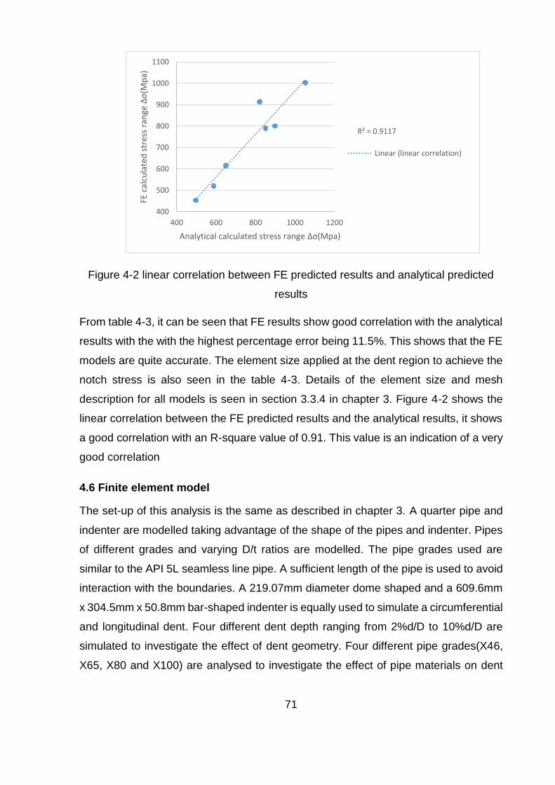
71

Figure 4-2 linear correlation between FE predicted results and analytical predicted

results

From table 4-3, it can be seen that FE results show good correlation with the analytical

results with the with the highest percentage error being 11.5%. This shows that the FE

models are quite accurate. The element size applied at the dent region to achieve the

notch stress is also seen in the table 4-3. Details of the element size and mesh

description for all models is seen in section 3.3.4 in chapter 3. Figure 4-2 shows the

linear correlation between the FE predicted results and the analytical results, it shows

a good correlation with an R-square value of 0.91. This value is an indication of a very

good correlation

4.6 Finite element model

The set-up of this analysis is the same as described in chapter 3. A quarter pipe and

indenter are modelled taking advantage of the shape of the pipes and indenter. Pipes

of different grades and varying D/t ratios are modelled. The pipe grades used are

similar to the API 5L seamless line pipe. A sufficient length of the pipe is used to avoid

interaction with the boundaries. A 219.07mm diameter dome shaped and a 609.6mm

x 304.5mm x 50.8mm bar-shaped indenter is equally used to simulate a circumferential

and longitudinal dent. Four different dent depth ranging from 2%d/D to 10%d/D are

simulated to investigate the effect of dent geometry. Four different pipe grades(X46,

X65, X80 and X100) are analysed to investigate the effect of pipe materials on dent

R² = 0.9117

400

500

600

700

800

900

1000

1100

400 600 800 1000 1200

FE c

alcu

late

d s

tres

s ra

nge

∆σ

(Mp

a)

Analytical calculated stress range ∆σ(Mpa)

Linear (linear correlation)

72

fatigue. Similarly, eight pipes with a different diameter to thickness ratio D/t ranging

from 18-96 are analysed to investigate the effect of pipe geometry as seen in table 3-

1. Finally, two ranges of pressure (50% and 72%SMYS) are applied to the pipe to see

the effect of pressure range. The material modelling is the same as described in section

3.2.2 in chapter 3. Similarly the elements used is the same as described in section

3.2.3. The meshing procedure and the boundary conditions are the same as described

in section 3.2.4 and 3.2.5 respectively.

4.6.1 Loading

In a typical offshore and onshore environment, pipelines may be subjected to other

loads such as high temperature and external pressure. To simplify the model, such

loads are not accounted for and as such are not included in the loading procedure

The loading took the following sequence;

1. Displacement is applied on the indenter to create a dent with the depth higher

than the required dent depth

2. The indenter is removed to allow spring back with the spring back depth being

the measured dent depth.

3. Internal pressure is applied to the internal surface of the pipe. An initial pressure

of 80% MOP is applied, afterwards, a pressure range of between 0 to

50%SMYS and 72%SMYS is applied

4. The internal pressure is removed to determine reround depth.

It is assumed that dents are introduced at zero pressure. The required dent depths

are the ones measured after spring back. It is difficult to get the exact dent depth after

spring back; however, the values measured are as close to the required depth. A

pressure range of 0 to 50%SMYS and 0 to 72%SMYS is applied on the internal pipe

walls and the SCF is computed at 50% and 72%SMYS pressure ranges. The pressure

is then removed to see the residual depth.

It is important to know the type of stress to be recorded as different SN curves use a

different type of stresses. The notch stresses recorded in this study are the maximum

73

principal stresses as used in the DOE B-curve [106] and these stresses can be gotten

by following the modelling procedure as described in section 3.3 in chapter 3 and by

using the correct element size as shown in table 3-3 and 3-4.

4.6.2 Variables considered

As discussed in the literature review, factors that affect the accurate prediction of stress

include pipe geometry, which is presented by the diameter to thickness ratio (D/t), the

dent length to external diameter ratio (L/D), and dent depth to pipe diameter ratio (d/D),

pipe material and pressure range. These variables are used as input data for an

artificial neural network which is discussed later in chapter 6. Table 4-3 shows these

variables.

D/t 18.6, 25, 32, 40,

50, 62, 80, 90

Pipe grades X46, X65, X80,

X100

Ho(%) 2, 5, 7, 10

Indenter type Dome and Bar

Pressure(% SMYS) 50, 72

Table 4-4 variables considered

4.6.3 Parametric study

In order to adequately predict the SCF with an artificial neural network, a parametric

data sets of the inputs and output variables are needed. This has led to a parametric

study which is conducted on a variety of pipe with different pipe materials, dent shape

and dent depths to extract the SCF associated with each dent scenario. The SCFs are

extracted by dividing the stress range over the pressure range. The SCF can then be

used with DOE-B curve to calculate the fatigue life with equation (4-1).

74

4.7 Results

4.7.1 Stress locations

The results from this study shows that stress concentration factor is influenced by the

pipe geometry, dent geometry, pipe material and pressure range. When the pipes are

dented, there is an increase in the stress concentration in the dented areas. The

location of the maximum stress is found around the dented region and can either be at

rim or root of the dent. The location of the maximum stress is dependent on the length

to width ratio of the dent. Figures 4-3 and 4-4 represent a typical dent profile of a Dome

and bar indenter model for an X46 pipe grade. This profile was measured at the end

of the second load step during the loading sequence. The profile for a 2%, 5%, 7%

and 10% dent depth are included in the figures. Figures 4-5 and 4-6 show the location

of maximum stress for a dome and bar model respectively. The location of the

maximum stress is the likely region of the formation of crack, which can propagate and

eventually lead to failure. As cyclic pressure is applied on the pipe, the location of the

maximum 1st principal stress is dependent on the pipe geometry, dent geometry and

pipe material. However, they are all found at the dent region.

Figure 4-3 Dome dent profile for an X46 pipe grade

0

5

10

15

20

25

30

0 500 1000 1500 2000 2500 3000

d(m

m)

L(mm)

Dome dent profile

10%

7%

5%

2%

75

Figure 4-4 Bar dent profile for an X46 pipe grade

Figure 4-5 maximum stress location for a dome dent

0.00E+00

5.00E+00

1.00E+01

1.50E+01

2.00E+01

2.50E+01

3.00E+01

0 500 1000 1500 2000 2500 3000

d(m

m)

L(mm)

Bar dent profile

10%

7%

5%

2%

76

Figure 4-6 Maximum stress location for a bar dent

4.7.2 Effect of pipe geometry on SCF

From past literature, the pipe geometry has been seen to influence the stress

concentration factor. Results from this study indicate that stress concentration factor

increases with increasing diameter to thickness ratio D/t. This, in turn, will give a

corresponding decrease in the fatigue life. Both the dome and bar dent show that

Stress concentration factor increased as D/t increased. Figure 4-6 below shows the

effect of pipe geometry for a 2% dome and bar indenter models for all pipe grades. It

can be seen that the SCF appears to increase in a linear manner for both the bar and

dome models for all pipe grades. The SCFs are plotted for both the 50% and

72%SMYS pressure range. Appendix C.1.1 and C.1.2 also shows the effect of pipe

geometry on SCF on the other dent depths and they all show similar pattern.

77

(a) 2% d/D at 72SMYS for dome dent

(b) 2%d/D at 50% SMYS for dome dent

0

20

40

60

80

100

120

0 20 40 60 80 100 120

∆σ

/∆p

D/t

X46

X65

X80

X100

0

20

40

60

80

100

120

0 20 40 60 80 100 120

∆σ

/∆p

D/t

X46

X65

X80

X100

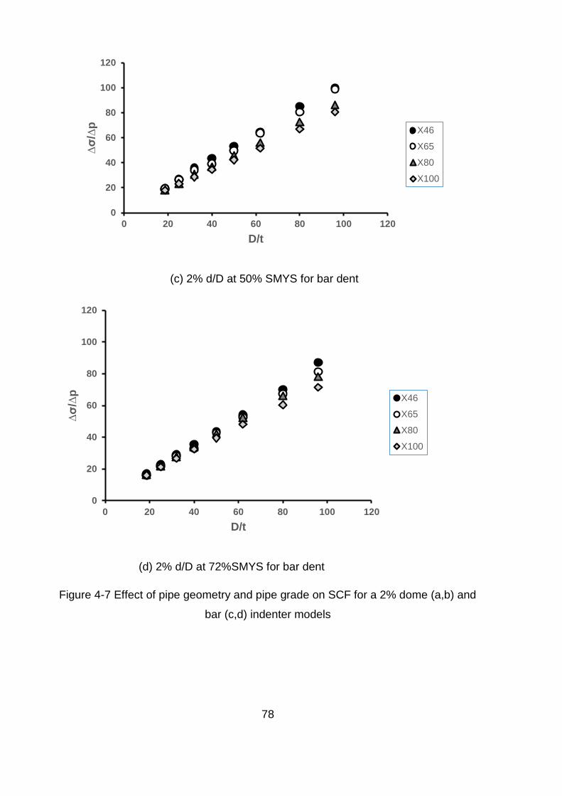
78

(c) 2% d/D at 50% SMYS for bar dent

(d) 2% d/D at 72%SMYS for bar dent

Figure 4-7 Effect of pipe geometry and pipe grade on SCF for a 2% dome (a,b) and

bar (c,d) indenter models

0

20

40

60

80

100

120

0 20 40 60 80 100 120

∆σ

/∆p

D/t

X46

X65

X80

X100

0

20

40

60

80

100

120

0 20 40 60 80 100 120

∆σ

/∆p

D/t

X46

X65

X80

X100

79

4.7.3 Effect of pipe grade on SCF

Results from this study show that the material grade in terms of the specified minimum

yield stress 'SMYS' can influence the fatigue life of a pipe with dents. Results show

that pipes with higher material strengths have higher notch stresses compared to the

lower pipe grades. This can be seen in table 4-3 in section 4.5. However, the ratio of

the stress range over the pressure range ∆σ/∆p appears higher in the lower pipe

grades compared to the higher pipe grades as shown figure 4-7. This appears to be

true for other dent depth as seen in appendix C.1.1 and C.1.2. This effect could be

attributed to the fact that the operating pressure is a function of the pipe’s yield

strength, diameter and thickness. Pipes with higher strength have higher operating

pressure magnitude. When pipes with higher material strengths are pressurised, there

is increased rerounding due to the increased pressure magnitude. As a consequence,

the dent depth is reduced thereby reducing its susceptibility to higher stress

concentration. Observations from the results show that the difference in ratio(∆σ/∆p)

between pipe grades are smaller for pipes with smaller D/t. However, the difference in

ratio between pipes grades increases as D/t increases further. It can also be seen from

figure 4-7 that the difference is more for 50%SMYS pressure range compared to the

72% SMYS range.

4.7.4 Effect of dent geometry on SCF

The results from this study also show that longitudinal dents exhibit higher SCF

compared to a circumferential dent. Figure 4-8 shows plots for both longitudinal and

circumferential dents for an 18.6 D/t ratio and X46 pipe grade. The SCFs are plotted

against the dent depth. These plots show that SCF is higher in the longitudinal dent of

same dent depth. From the result, it is also clear that dent with higher dent depth

exhibits higher stress concentration factor. Other pipe grades and D/t show similar

pattern.

80

Figure 4-8 Effect of dent geometry

4.7.5 Effect of mean internal pressure

The result shows that internal pressure range can affect stress concentration. An

internal pressure range of up to 50% and 72% SMYS is applied to the pipe. Results

from this study indicate that SCF is higher in the 50% SMYS pressure range compared

to the 72% SMYS pressure range. This is so because, as internal pressure is applied

to the pipe wall, the dent begins to reround. As internal pressure is applied further, the

dent depth is reduced accordingly, which leads to less stress concentration around the

dent region. Figures 4-9 and 4-10 show the effects of pressure range for a 2% dent

depth with X46 material for dome and bar dent.

0

2

4

6

8

10

12

14

16

18

20

0 2 4 6 8 10 12

∆σ

/∆p

D/t

18.6 D/t, X46, 72% SMYS

dome

bar

81

Figure 4-9 Effect of pressure range for a 2% d/D, X46 dome dent

(b)

Figure 4-10 Effect of pressure range for a 2% d/D, X46 bar dent

0

20

40

60

80

100

120

0 20 40 60 80 100 120

∆σ

/∆p

D/t

50%SMYS

72%SMYS

0

20

40

60

80

100

120

0 20 40 60 80 100 120

∆σ

/∆p

D/t

50%SMYS

72%SMYS

82

4.8 Summary of results and conclusions

As part of a study to develop an algorithm for the evaluation of dent severity and

fatigue, this study extracts stress concentration factor (SCF) from dome and bar dents

under cyclic loading. A parametric range of industry pipes is analysed under various

conditions to see its effect on dent severity. Result from this study has shown that

Pipes with higher material strength exhibit higher notch stresses compared to

pipes with lower material strength . However, due to the effect of the operating

pressure, the ratio of the stress range to the pressure range(∆σ/∆p) appears

lower for pipes with higher material strength. The results also show that the

difference in SCF between pipe grades are smaller for pipes with smaller D/t.

However, the difference in SCF between pipes grades increases as D/t

increases further. It can also be seen from the result that the difference is more

for 50%SMYS pressure range compared to the 72% SMYS range.

Stress concentration increases with increasing pipe D/t ratio

Bar dents show higher stress concentration compared to dome dents. It is also

clear from the result that dent with higher dent depth exhibit higher stress

concentration factor.

SCF is higher in the 50% SMYS pressure range compared to the 72% SMYS

pressure range. This is so because, as internal pressure is applied to the pipe

wall, the dent begins to reround. As internal pressure is applied further, the dent

depth reduces thereby reducing the stress concentration around the dent region

The results were validated with experimental and analytical solutions and they both

show good correlation. This shows that the FE models are quite accurate and can be

confidently used to develop the ANN models. The parametric dataset from the FEA

study is used to train an artificial neural network using the parameters as input data to

predict the SCF.

83

CHAPTER 5

STRAIN-BASED ASSESSMENT OF PLAIN DENTS

5.1 Introduction

Over the years, dent depth was used by various codes to determine dent severity.

These codes include ASME 2006, DNV 2007, EPRG. Recent studies have however

shown that dent depth alone is not sufficient enough to determine the severity of dents.

The local strain concentration in the pipe has been found to be a better predictor of

dent severity. As a result, ASME introduced a strain based assessment in its 2004

version of the ASME B31.8 code. This code also provides a formula for calculating the

total strain. This code accepts dent of any depth as long as the associated strain level

does not exceed 6%. The ASME code only considers the dent geometric properties.

However, just like the stress approach, there is another parameter that may influence

the strain in the pipeline. This parameter is the pipe grade . This study will investigate

these parameters and how they influence the prediction of strain in the pipeline. The

objectives of this chapter include

Improving the understanding of strain distribution in pipeline with dents

Identifying the most important parameters which influence the strain in dents

Creating database for development of an ANN-based formula in chapter 6 using

the above parameters

The purpose of this chapter is to create an alternative method to the ASME B31.8

formula for the strain-based assessment. The ANN-formula include the effect of pipe

grades as opposed to the ASME formula that only considers the geometric properties

of the pipe and dent. The ANN-based formula provides a more comprehensive method

for calculating the maximum strain as it looks into all the parameters considered by

ASME and also looking at an additional parameter not considered by ASME. The

proposed procedure for calculating strain in dent is discussed in chapter 7.

5.2 Current method for estimating strain in pipeline

Strain act on both the longitudinal and circumferential axis of a pipe and each axis have

two types of strain acting on them. They include the bending and membrane strain.

84

According to the ASME B31.8 document [19], the maximum strain in dent is estimated

by first evaluating each strain component separately then assuming each component

occur coincidentally at the dent apex, the components are combined to give the total

strain. The membrane strain is constant throughout the pipe wall but the circumferential

strain varies through the pipe wall about the neutral axis. The bending strain in the

circumferential direction (ε1) and the bending and membrane strains in the longitudinal

direction (ε2 and ε3) are shown in the equations 5-1, 5-2 and 5-3

𝜀1 = (𝑡

2) (

1

𝑅0−

1

𝑅1) (5-1)

𝜀2 = −(𝑡

2) (

1

𝑅2) (5-2)

𝜀3 = (1

2) (

𝑑

𝐿)2

(5-3)

Where t, d and L are the wall thickness, dent depth and dent length in the longitudinal

direction respectively; Ro is the radius of curvature of the undeformed pipe surface

(equal to half of the nominal pipe outside diameter): R1 and R2 are radii of curvature

measured in the transverse and longitudinal planes through the dent. This is depicted

in figure 5-1.

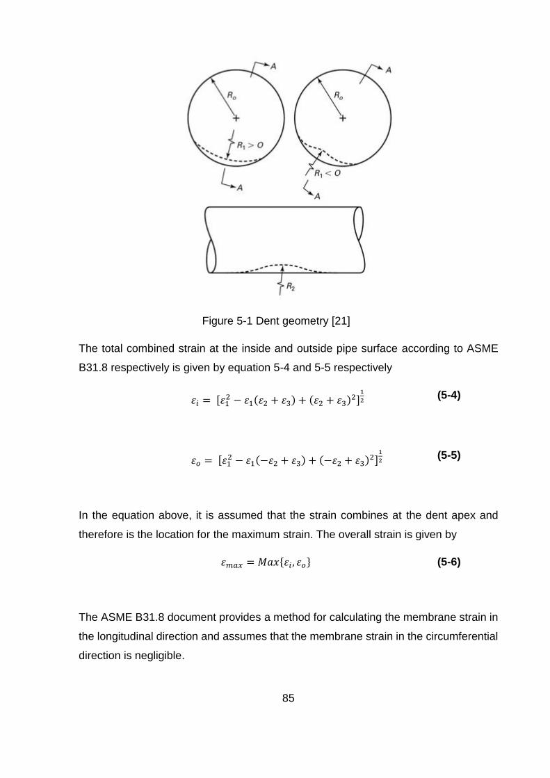
85

Figure 5-1 Dent geometry [21]

The total combined strain at the inside and outside pipe surface according to ASME

B31.8 respectively is given by equation 5-4 and 5-5 respectively

𝜀𝑖 = [𝜀12 − 𝜀1(𝜀2 + 𝜀3) + (𝜀2 + 𝜀3)

2]1

2 (5-4)

𝜀𝑜 = [𝜀12 − 𝜀1(−𝜀2 + 𝜀3) + (−𝜀2 + 𝜀3)

2]1

2 (5-5)

In the equation above, it is assumed that the strain combines at the dent apex and

therefore is the location for the maximum strain. The overall strain is given by

𝜀𝑚𝑎𝑥 = 𝑀𝑎𝑥{𝜀𝑖, 𝜀𝑜} (5-6)

The ASME B31.8 document provides a method for calculating the membrane strain in

the longitudinal direction and assumes that the membrane strain in the circumferential

direction is negligible.

86

Noronha Jr et al [21], however, demonstrated that the ASME B31.8 [19] equations

were derived considering incorrect plane strain assumptions and therefore their use

can lead to inaccurate results. They came up with new equations to calculate the

combined strain considering the plain strain state which are :

𝜀𝑖 = 2

3[𝜀1

2 − 𝜀1(𝜀2 + 𝜀3) + (𝜀2 + 𝜀3)2]

1

2 (5-7)

𝜀𝑜 = 2

3[𝜀1

2 − 𝜀1(−𝜀2 + 𝜀3) + (−𝜀2 + 𝜀3)2]

1

2 (5-8)

It can be observed that the equations are similar to that of the ASME equations except

for the fact that they are preceded by the constant (2/3). They argued that in the

derivation of the equations, the assumption that the radial strains are negligible is

questionable since it means that at the dent region, the pipe wall is subjected to plane

strain state, which is not true. They further went ahead to develop equations for the

combined strain considering the radial components with the remit that strains in this

region are mainly in the plastic range where the incompressibility condition may be

applied. The modified equations considering the radial components are as follows

𝜀𝑖 = 2

√3√𝜀1

2 + 𝜀1(𝜀2 + 𝜀3) + (𝜀2 + 𝜀3)2

(5-9)

𝜀𝑜 = 2

√3√𝜀1

2 − 𝜀1(−𝜀2 + 𝜀3) + (−𝜀2 + 𝜀3)2

(5-10)

They compared the results from these equations to that of a finite element study and

the results were in close agreement as opposed to the ASME equation which under

predicted the strain

87

5.3 Finite Element Model

Similar to the SN approach, a finite element model is used to investigate the effect of

parameters like dent geometry, pipe geometry and pipe grade on the strain distribution

in dented pipeline.

The model used is similar to the one used for the SN approach. It uses a non-linear

elastic-plastic finite element analysis for the study. The geometry creation is the same

as described in section 3.2.1 in chapter 3. A quarter model of both the pipe and indenter

are modelled taking advantage of the symmetry of the pipe and indenter. The material

modelling is also the same as described in section 3.2.2. Four different pipe grades

are used to determine the effect of pipe material on the strain distribution in the

pipeline. 8 different pipes with varying diameter to thickness ratio D/t as seen in table

3-1 in chapter 3. Two types of indenter (Dome and bar) are used to simulate

circumferential and longitudinal dents respectively. The element used and the meshing

procedure are the same as described in section 3.2.3 and 3.2.4 respectively. The same

element size as described in table 3-3 and 3-3 is used to achieve the notch strain.

Similarly, the boundary conditions are the same as described in section 3.2.5.

5.3.1 Loading

The loading took the following sequence

1. The pipe is indented at zero pressure to a depth higher than the expected dent

depth. This is done because the pipe is expected to experience some spring

back and the spring back depth is the measured dent depth

2. The indenter is then removed to allow spring back in the pipe

It is important to note that the dent depth considered for this assessment is the dent

depth after spring back and can be viewed as a construction dent. However an ANN-

based formula is given in chapter 6 that gives the relationship between spring back

depth and reround depth considering various parameters.

5.3.2 Parametric study

A parametric study is conducted to evaluate the effect of the various parameters

including, dent geometry, pipe geometry and pipe grade that might affect the strain

prediction in the pipe. As discussed earlier, the current method for assessing strain as

88

proposed by ASME only considers the geometric properties of the pipe. This study

aims to consider the other parameters that might influence the strain in the pipeline. In

order to this, 8 different pipes with D/t ranging between 18.5 to 96 are modelled to

study the effect of pipe geometry, 4 different dent depths are considered to study the

effect of dent geometry on the strains. Similarly, 4 different pipe grades are used to

study the effect of pipe material. The table showing these variables is seen in table 4-

1 in chapter 4. The parametric data set obtained from this study is eventually used to

train an artificial neural network ANN to predict the strain in the pipeline.

5.4 Effect of important variables on strain

As discussed earlier, two components of strain act in a pipeline; the circumferential

and longitudinal strain. The total strain in the pipeline is a combination of the two

strains. Circumferential, longitudinal. The location of the maximum strain is found at

the dent apex for both the dome and bar indenter model as seen in figure 5-2 and 5-3

respectively. The maximum strains recorded are obtained during spring back at zero

pressure The strain values extracted from the FEA study are the equivalent Von Mises

strain. Table 5-1 and 5-2 shows the total strain recorded at spring back for the dome

and bar indenter models respectively. From the results, it is seen that the various

parameters affect the strain as is discussed below

89

Figure 5-2 Location of maximum strain after spring back for dome indenter

Figure 5-3 Location of maximum strain after spring back for a bar indenter

D/t X46 X65 X80 X100

d/D (%)1 Dome d/D(%)1 Dome d/D(%)1 Dome d/D(%)1 Dome

εt εt εt εt

18.6 1.9 0.099 1.6 0.087 2.3 0.118 1.9 0.099

25 1.8 0.1 2 0.11 1.6 0.098 1.8 0.1

32 2.2 0.123 1.8 0.11 2.2 0.13 2.2 0.123

40 1.7 0.11 1.6 0.1 2.2 0.13 1.7 0.11

50 1.8 0.104 1.6 0.098 2.3 0.115 1.8 0.104

90

62 1.8 0.091 2.5 0.086 2.2 0.092 1.8 0.091

80 2.2 0.069 2.3 0.067 2.6 0.067 2.2 0.069

96 1.9 0.05 2.1 0.049 2.6 0.051 1.9 0.05

18.6 4.9 0.15 4.5 0.15 5 0.16 4.9 0.15

25 5.7 0.186 4.6 0.16 5.4 0.2 5.7 0.186

32 4.3 0.158 4.6 0.147 5 0.18 4.3 0.158

40 5.3 0.14 4.6 0.13 5.1 0.156 5.3 0.14

50 4.4 0.112 4.7 0.104 5.5 0.118 4.4 0.112

62 5 0.091 4.8 0.087 5.8 0.092 5 0.091

80 4.6 0.069 5.5 0.065 5.5 0.066 4.6 0.069

96 4.9 0.049 5.6 0.048 5.6 0.05 4.9 0.049

18.6 7.2 0.185 7 0.18 7.8 0.198 7.2 0.185

25 6.9 0.19 7.3 0.17 7.5 0.21 6.9 0.19

32 6 0.165 6.6 0.15 7.2 0.18 6 0.165

40 6.7 0.14 6.9 0.129 7.4 0.155 6.7 0.14

50 7 0.109 6.6 0.103 7.7 0.117 7 0.109

62 6.9 0.086 6.9 0.083 7.7 0.091 6.9 0.086

80 7 0.064 7 0.063 7.5 0.066 7 0.064

96 7 0.049 7.6 0.049 7.7 0.05 7 0.049

18.6 9.6 0.196 9.1 0.19 10.2 0.21 9.6 0.196

25 9.5 0.19 10.1 0.17 10.8 0.21 9.5 0.19

32 9.1 0.165 9.9 0.15 10.5 0.18 9.1 0.165

40 10.3 0.14 9.6 0.13 10.5 0.157 10.3 0.14

50 9.4 0.109 9.9 0.1 10.8 0.118 9.4 0.109

62 9.7 0.085 10.5 0.082 10.6 0.091 9.7 0.085

91

80 9.8 0.065 10 0.06 10.6 0.066 9.8 0.065

96 9.9 0.049 10.8 0.049 11.3 0.057 9.9 0.049

1 Measured dent depth after spring back

Table 5-1 Total strain measured at spring back for dome indenter models

D/t X46 X65 X80 X100

d/D (%)1 Bar d/D(%)1 Bar d/D(%)1 Bar d/D(%)1 Bar

εt εt εt εt

18.6 1.8 0.13 1.9 0.13 1.9 0.15 1.5 0.13

25 1.9 0.095 1.9 0.094 1.8 0.1 1.7 0.095

32 2.1 0.069 1.9 0.069 2 0.077 1.8 0.069

40 2.1 0.049 1.9 0.051 1.9 0.054 2 0.052

50 1.9 0.037 1.8 0.04 1.9 0.04 1.9 0.04

62 2.2 0.034 1.9 0.036 2.1 0.03 1.8 0.032

80 1.6 0.025 2.1 0.029 2.1 0.028 1.6 0.024

96 1.8 0.024 2.4 0.024 1.9 0.023 1.5 0.019

18.6 5 0.245 4.7 0.208 5.3 0.27 4.6 0.024

25 4.8 0.157 4.7 0.145 5 0.175 5 0.16

32 5.1 0.11 4.8 0.104 5 0.117 5.3 0.109

40 5.3 0.077 4.8 0.072 4.9 0.075 5.3 0.068

50 4.8 0.054 4.7 0.05 5.4 0.054 5.1 0.05

62 5.1 0.041 5.3 0.047 6 0.062 4.5 0.045

80 4.6 0.031 5.3 0.05 5.6 0.067 4.6 0.05

96 5.1 0.036 5.2 0.047 5.9 0.062 4.4 0.046

18.6 7.1 0.27 6.5 0.22 7.3 0.029 7.1 0.0275

92

25 7.4 0.178 6.7 0.159 7 0.188 7.2 0.175

32 7.4 0.12 6.2 0.11 6.9 0.123 7.1 0.11

40 7.3 0.081 7 0.076 7.5 0.08 7 0.072

50 6.3 0.057 7.2 0.072 7.8 0.094 7 0.084

62 7.3 0.056 6.8 0.061 7.3 0.07 6.3 0.064

80 6.3 0.049 7.7 0.084 6.7 0.085 6.3 0.082

96 6.8 0.05 7.5 0.067 7.6 0.076 7.3 0.068

18.6 10.5 0.029 9.8 0.24 9.5 0.31 10 0.29

25 9.6 0.18 10.2 0.167 9.7 0.19 10.2 0.19

32 10.1 0.13 10.6 0.14 9.9 0.16 10.4 0.167

40 10.6 0.103 8.7 0.086 10.6 0.13 10.2 0.129

50 11.4 0.11 9.1 0.097 11 0.136 9.7 0.118

62 9.6 0.076 9.8 0.09 11.2 0.122 10.3 0.11

80 10.5 0.106 10 0.11 10.6 0.13 9 0.114

96 11 0.076 11 0.08 11.4 0.09 10.5 0.084

1 Measured dent depth after spring back

Table 5-2 Total strain measured at spring back for bar indenter models

5.4.1 Effect of pipe geometry on strain

Pipe geometry is one of the parameters that influence the strain concentration in the

pipeline. From the result, it is seen that the circumferential, longitudinal and total strain

reduces as the diameter to thickness ratio (D/t) of the pipe increases. Figure 5-4 and

5-5 below represents a graph showing the effect of the diameter to thickness ratio (D/t)

of the pipe on strain for a dome and bar indenter model respectively. It shows the result

of a 5% dent depth for an equivalent pipe grade. From Figure 5-4, it is seen that the

circumferential strain is higher than the longitudinal strain and decreases as the D/t

increases. However, figure 5-5 shows the opposite with the longitudinal strain higher

than the circumferential strain. A plot of other dent depths can be seen in appendix D

93

and they all show similar trend. From this results, one can conclude that circumferential

dents have a higher strain in the circumferential direction and the longitudinal dents

have a higher strain in the longitudinal direction compared to the circumferential

direction. A particular observation from the results shows that the difference between

the circumferential and longitudinal strain is higher in circumferential dent compared to

that of the longitudinal dent.

Figure 5-4 Effect of pipe geometry on strain for a 5% dome dent for X46 pipe grade

Figure 5-5 Effect of pipe geometry on strain for a 5% bar dent for X46 pipe grade

0.00

0.02

0.04

0.06

0.08

0.10

0.12

0.14

0.16

0.18

0.20

0 20 40 60 80 100 120

max s

train

D/t

circumferential strain

longitudinal strain

total strain

0.00

0.05

0.10

0.15

0.20

0.25

0.30

0 20 40 60 80 100 120

ma

x s

train

D/t


longitudinal strain

total strain

94

5.4.2 Effect of dent geometry on strain

The dent orientation and dent depths are some of the parameters that affect the strains

in the pipeline. This section investigates how these parameters influence the strain

distribution. The result from the study has shown that the total strain in a dent is higher

in a longitudinal dent compared to a circumferential dent. Figure 5-6 shows a graph of

strain versus the dent depth for both the longitudinal and circumferential dent for an

18.5 D/t. It clearly shows the longitudinal dent at the top of the graph indicating higher

strain. Similarly, an increase in dent depth gives a corresponding increase in the strain

for both dent models. The dent geometry also determines the location of the maximum

strain. Though the maximum strain is situated at the apex of the dent depth as seen in

figure 5-2 and 5-3, the location of the strains are different for each dent type. The

maximum strain is located at the bottom of the dent and is centralised for a dome dent,

however, the bar dent has the maximum strain located at the far end of the dent.

Figure 5-6 Effect of dent geometry on strain for an 18.6 D/t for all dent depths and

pipe grades

0.00

0.05

0.10

0.15

0.20

0.25

0.30

0.35

0 2 4 6 8 10 12

max s

train

d/D(%)

X46 Dome

X46 bar

X65 dome

X65 bar

X80 dome

X80 bar

X100 dome

X100 bar

95

5.4.3 Effect of pipe grades on strains

As discussed earlier in the chapter, the ASME method for evaluating strains in dent

only considers the geometric properties of the pipe dent. Studies have shown that other

parameters like pipe grades can influence the strain prediction in the pipe. This study

investigates the effect of the pipe grades on the magnitude and distribution of the

strains in the pipeline. Figure 5-7 and 5-8 below shows a plot of the strain versus the

D/t for a 10% dent depth for the four different pipe grades. Figure 5-7 represents plots

for the dome indenter and figure 5-8 represents plots for the bar indenter. From figure

5-7, a noticeable difference is seen in the strain magnitude up until a D/t of 50. Though

it does not follow a definite pattern, the higher pipe grades appear to have higher strain.

As the D/t increases further, the difference in the strain are quite small. Other dent

depth appears to follow the same pattern for the dome dent as seen in appendix D.2.

Figure 5-8, however, doesn’t follow a particular pattern. Some of the dent depths as

shown in appendix D.2 shows a minimal difference in the strain for all pipe grades.

One of the parameters that might cause the irregular pattern observed here is the dent

depth, the measured dent for each pipe grades are different, and the dent depth has

been observed to be a critical factor in influencing the strain.

Figure 5-7 Effect of pipe grade on strain for a 10% dome dent

0.00

0.05

0.10

0.15

0.20

0.25

0 20 40 60 80 100 120

ma

x s

train

D/t

X46

X65

X80

X100

96

Figure 5-8 Effect of pipe grade on strain for a 10% bar dent

5.4.4 Comparison between ASME B31.8 , Modified ASME [21] and FEA

predicted strain

This section compares the total strain predicted using the ASME equation, Noronha et

al [21] and the predicted FEA strain. To do the comparison, the strain data extracted

from the X65 grade models are used, the dent depth of 2%, 5%, 7% and 10% for all

diameter to thickness ratios (D/t) are compared. Table 5-3 below compares the total

strain at the outer surface of the pipe between the FEA predicted strain, the ASME

predicted strain and Noronha et al[21] using the equations as described in equations

5-5 and 5-10 respectively. The dome indenter model is used to do the comparison.

Figure 5-9 also shows the graph of FEA predicted strain versus ASME predicted strain

and Noronha et al predicted strain.

D/t Diameter

(mm)

Thickness

(mm)

Measured

dent depth

(%)

FEA

predicted

strain

ASME predicted

strain[19]

Noronha et al

[21]

Strain

value

% error Strain

value

%

error

18.6 323.62 17.399 1.6 0.087 0.12 33.58 0.10 16.82

0.00

0.05

0.10

0.15

0.20

0.25

0.30

0.35

0 20 40 60 80 100 120

max s

train

D/t

Effect of pipe grade for 10% bar

X46

X65

X80

X100

97

25 323.62 12.944 2 0.11 0.09 21.35 0.11 2.20

32 323.62 10.1131 1.8 0.11 0.07 38.62 0.12 9.49

40 323.62 8.0905 1.6 0.1 0.05 46.01 0.10 2.90

50 323.62 6.4724 1.6 0.098 0.04 55.93 0.09 13.46

62 323.62 5.2196 2.5 0.086 0.03 59.48 0.08 7.31

80 323.62 4.04525 2.3 0.067 0.03 59.70 0.06 12.79

96 323.62 3.371 2.1 0.049 0.02 54.09 0.05 5.29

18.6 323.62 17.399 4.5 0.15 0.12 22.22 0.14 7.15

25 323.62 12.944 4.6 0.16 0.09 45.79 0.16 2.48

32 323.62 10.1131 4.6 0.147 0.07 53.97 0.14 8.63

40 323.62 8.0905 4.6 0.13 0.05 58.41 0.11 14.51

50 323.62 6.4724 4.7 0.104 0.04 58.43 0.10 9.35

62 323.62 5.2196 4.8 0.087 0.03 59.93 0.08 13.44

80 323.62 4.04525 5.5 0.065 0.03 58.42 0.06 4.57

96 323.62 3.371 5.6 0.048 0.02 53.09 0.05 1.51

18.6 323.62 17.399 7 0.18 0.12 35.41 0.21 13.98

25 323.62 12.944 7.3 0.17 0.09 49.12 0.16 9.18

32 323.62 10.1131 6.6 0.15 0.07 54.96 0.14 11.00

40 323.62 8.0905 6.9 0.129 0.05 58.09 0.12 8.46

50 323.62 6.4724 6.6 0.103 0.04 58.03 0.10 8.29

62 323.62 5.2196 6.9 0.083 0.03 57.98 0.08 3.48

80 323.62 4.04525 7 0.063 0.03 57.10 0.06 5.94

96 323.62 3.371 7.6 0.049 0.02 54.01 0.05 8.72

18.6 323.62 17.399 9.1 0.19 0.12 38.86 0.21 9.14

25 323.62 12.944 10.1 0.17 0.09 49.14 0.16 9.22

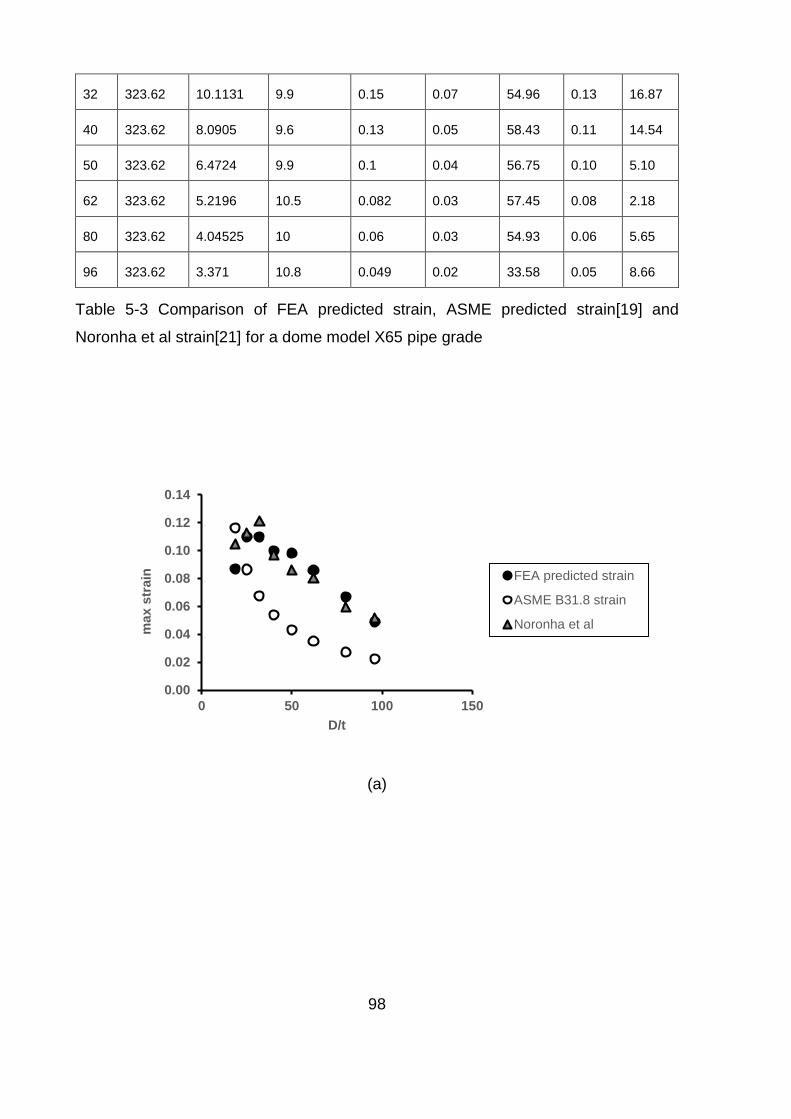
98

32 323.62 10.1131 9.9 0.15 0.07 54.96 0.13 16.87

40 323.62 8.0905 9.6 0.13 0.05 58.43 0.11 14.54

50 323.62 6.4724 9.9 0.1 0.04 56.75 0.10 5.10

62 323.62 5.2196 10.5 0.082 0.03 57.45 0.08 2.18

80 323.62 4.04525 10 0.06 0.03 54.93 0.06 5.65

96 323.62 3.371 10.8 0.049 0.02 33.58 0.05 8.66

Table 5-3 Comparison of FEA predicted strain, ASME predicted strain[19] and

Noronha et al strain[21] for a dome model X65 pipe grade

(a)

0.00

0.02

0.04

0.06

0.08

0.10

0.12

0.14

0 50 100 150

max s

train

D/t

FEA predicted strain

ASME B31.8 strain

Noronha et al

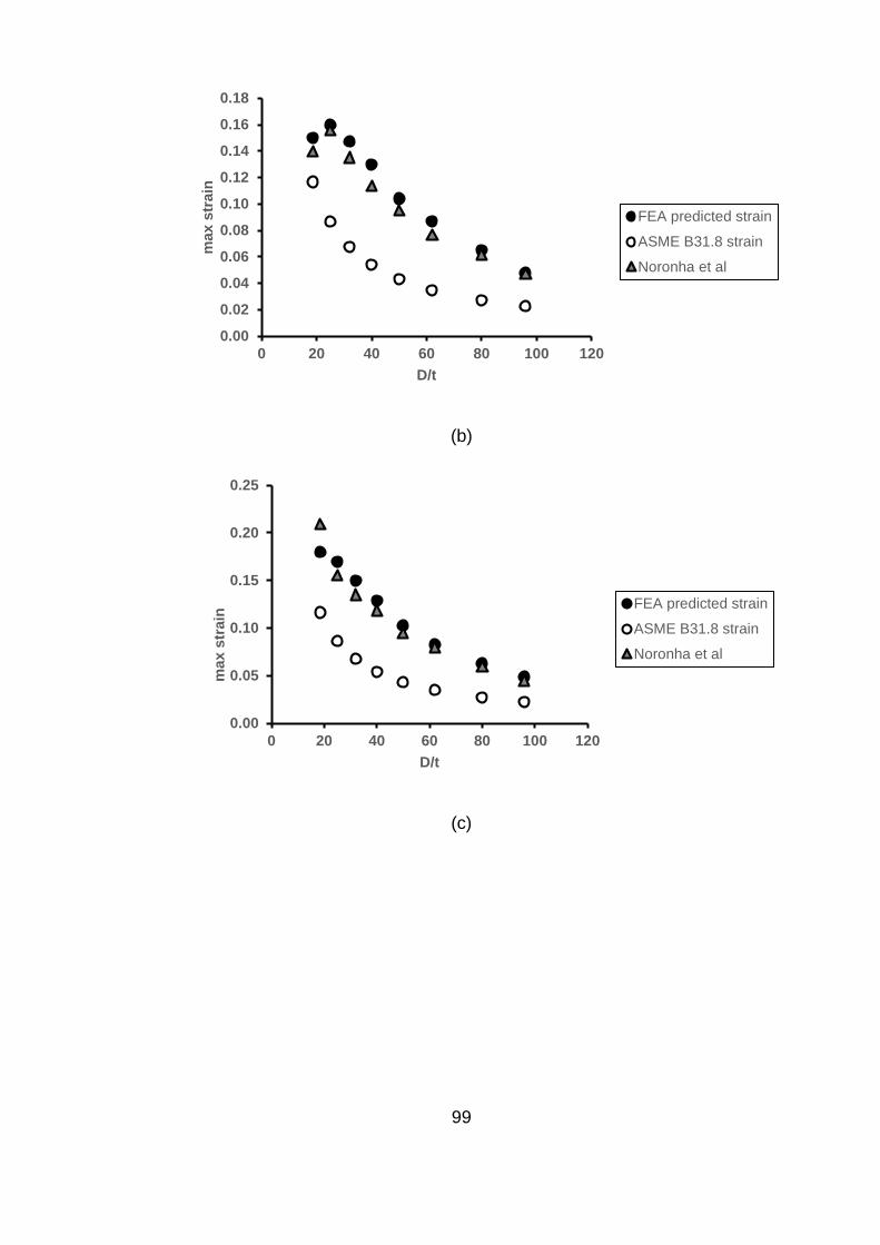
99

(b)

(c)

0.00

0.02

0.04

0.06

0.08

0.10

0.12

0.14

0.16

0.18

0 20 40 60 80 100 120

max s

train

D/t


ASME B31.8 strain

Noronha et al

0.00

0.05

0.10

0.15

0.20

0.25

0 20 40 60 80 100 120

ma

x s

train

D/t


ASME B31.8 strain

Noronha et al

100

(d)

Figure 5-9 Comparison of FEA predicted strain, ASME predicted strain[19] and

Noronha et al strain[21] for a 2%(a), 5%(b), 7%(c) and 10%(d) dent depth

From the results, it can be observed that all methods follow a similar pattern, however,

the ASME formula under-predicted the strain. The conservation in the ASME result

could be due to the fact that the ASME formula only considers the geometric properties

of the pipe and also does not consider the radial components of the strain. The formula

proposed by Noronha et al [21] however shows a very good correlation with the FE

results. This calls for a revision of the ASME B31.8 document. The notch strain is

achieved by following the modelling procedure as described in chapter 3. The element

size that was used to achieve the notch strain is seen in table 3-3 and 3-4

5.5 Summary of results and conclusion

The results above have shown how various parameters like pipe geometry, dent

geometry and pipe material can affect the total strain in the dent. These parameters

are very important in predicting the total strain. From the discussions presented above,

the below conclusions can be drawn

1. Circumferential strains are higher in circumferential dents compared to

longitudinal strains and reduce as the diameter to thickness ratio increases

0.00

0.05

0.10

0.15

0.20

0.25

0 20 40 60 80 100 120

max s

train

D/t


ASME B31.8 strain

Noronha et al

101

2. Longitudinal strains are higher in longitudinal dent compared to circumferential

strains and reduce as D/t increases

3. The difference between the circumferential and longitudinal strain is higher in

circumferential dent compared to that of the longitudinal dent.

4. The total strain in a dent is higher in a longitudinal dent compared to a

circumferential dent

5. As the dent depth increases, there is a corresponding increase in the strain for

both dent models

6. Pipes with higher material grades exhibits higher strain and the difference in

strain level gets smaller as the Diameter to thickness (D/t) increases

7. The ASME and the FEA predicted strain shows similarity in patterns in regards

to how the parameters affect the strain, however, the ASME equation under-

predicted the strain

8. The proposed formula by Noronha el al[21] gave a good correlation to the FEA

results

9. ASME needs to revise equation to consider the radial components of the strain

and also consider plane strain state

The objective of this chapter is to study the effect of these parameters on the strain

prediction. The data extracted from the FEA study is eventually used to train an

artificial neural network (ANN) in chapter 6 to be able to predict the maximum strain

level in the pipeline. The ANN-based formula will present a more comprehensive

method for evaluating the total strain in the dent as it includes the effect of pipe

grade which was not considered in the ASME equation.

103

CHAPTER 6

ARTIFICIAL NEURAL NETWORK APPLICATION FOR

PREDICTING REROUNDING, SCF AND STRAIN IN

DENTED PIPELINE

6.1 Introduction

Artificial neural network is a method than can be used to predict data through learning.

It derives its origin from the human nervous system which consist of a large parallel

interconnection of a large number of neuron. These neurons are interconnected in a

very complex way between each other to create a network. The artificial neural network

mimics a small part of the human brain to perform some specific task such as data

classification or pattern recognition through a learning process.

An artificial neural network consists of a set of neurons or processing element (PE)

that are connected by links of certain numeric weights. Each neuron has

a set of input links from other neurons

a set of output links from other neurons

a current activation function

an activation function to compute the activation level in the next time step

A typical neuron is seen in figure 2-7 in the literature review. From the figure x1, x2…xn

are the inputs, w1j, w2j….wnj are the weights. The total weighted input is the sum of

the input activation multiplied by their respective weights as shown by equation 6-1

𝐺 = ∑𝑊𝑖𝑗𝑥𝑖

𝑖=0

(6-1)

A typical neural network architecture will consist of an input layer, one or more hidden

layer, and an output layer. The input layer represents the information that is being fed

into the system. The hidden layer is dictated by the activities of the input units and the

104

weights between the input and hidden layer. The output layer relies on the action of

the hidden layer and weights between the input and output layer.

For this study, only one hidden layer is used because its efficiency is enough for this

application.

The number of neurons in the input layer is equal to the number of input variables,

similarly, the number of output layer is equal to the number of output variables. The

accuracy of the model is determined by the number of neurons in the hidden layer. The

relationship between the input xj and output yp of a single perceptron is given by the

expression below

𝑦𝑝 = 𝑓 (∑𝑤𝑝𝑗𝑥𝑗 + 𝑏𝑝

𝑁

𝑗=1

)

(6-2)

Where 𝑤𝑝𝑗 are the weights, bp is a constant usually referred to as bias and 𝑓( ) is the

activation function [6]. The number of weights and biases to be determined depends

on the network architecture itself. It can be determined by the equation (6-3).

(ni x nh) + (nh x no) + (nh +no)

(6-3)

Where ni is the number of inputs, nh is the number of processing elements in the hidden

layer and no is the number of output.

There are several algorithms that can be used to train a neural network. Some of them

include back-propagation, genetic algorithm, and particle swam optimisation. For this

study, the back propagation algorithm is used as it is the fastest and the most common

technique. It also gives insight on how the weights and biases can affect the behaviour

of the network.

Suppose we have an input layer X and an output layer Y with the transpose of the

vector of the input variables is XT = (x1, x2, x3,… xn ) and the transpose of the output

variable as YT = (y1, y2, y3,… yl). The mathematical expression between the input and

output is given by equation (6-4).

105

Y = 𝑓 {𝑊2𝑇x [

𝐼

𝑓 (𝑊1 x ⟨𝐼

𝑋⟩)]}

(6-4)

Where I is a unit one by one unit matrix and the expressions of matrices W1 and 𝑊2𝑇

are

W1 = [𝑏1

.𝑤𝑖ℎ1

1

.𝑤𝑖ℎ1

2 ⋯. .

𝑤𝑖ℎ1𝑛

.𝑏𝑚 𝑤𝑖ℎ𝑚

1 𝑤𝑖ℎ𝑚2 … 𝑤𝑖ℎ𝑚

𝑛]

(6-5)

𝑊2𝑇=[

𝑐1

.𝑤ℎ𝑜1

1

.𝑤ℎ𝑜1

2 ⋯. .

𝑤ℎ𝑜1𝑚

.𝑐𝐿 𝑤ℎ𝑜𝐿

1 𝑤ℎ𝑜𝐿2 … 𝑤ℎ𝑜𝐿

𝑚]

(6-6)

The behaviour of an ANN greatly depends on the activation function, weights, and

biases. There are different types of activation functions. The most common ones are

the logistic sigmoid and the hyperbolic tangent transfer functions. Both functions are

compared to determine the one that best predicts the SCF. The expressions for both

the logsig and hyperbolic tangent functions are given below

Logsig=Y=1

1+ 𝑒−𝑥

(6-7)

Hyperbolic tangent=Y=𝑒𝑥−𝑒−𝑥

𝑒𝑥+𝑒−𝑥

(6-8)

106

In this Study, ANN is used to predict the total rerounding, stress concentration factor

and the maximum strain in the dent. A commercial software MATLAB by

MATHWORKS is used to develop the model. The ANN architecture constitute of an

input layer with 4 input variable for the strain and rerounding model and 5 input

variables for the SCF models. It consist of one hidden layer and one output layer with

one output variable. The performance of the network is measured by alternating the

number of neurons in the hidden layer, the transfer functions, and the weights. The

ranges of the input variables are seen in table 6-1.

D/t d/D L/D σy Pmean

Dome Bar Dome Bar Dome Bar Dome Bar Dome Bar

Minimum 18.6 18.6 1.3 1.5 0.2163 2.9046 317 317 3.55 3.55

Maximum 96 96 11.3 11.4 3.6154 6.1183 690 690 48.07 48.07

Table 6-1 input variable ranges for ANN models

6.2 Constitutive ANN model for rerounding prediction

In this study, artificial neural network is used is to predict the reround depth of a dent

in a pipeline. Two separate models are developed to predict the dome dents and bar

dents. There are several training algorithms that can be used to train the data. It is

difficult to determine the training algorithm that will be fastest for a given problem. The

speed is dependent on many factors such as the number of data points in the training

set, the complexity of the problem, the number of weights and biases, error goals and

whether or not the network is being used for pattern recognition or regression. For this

study, the Levenberg-Marquardt function is used as it the most common training

function and has been proven to give good fits. The network will have one hidden layer

as this is sufficient enough to perform the analysis. However, different number of

processing elements are varied to determine the one that gives the best performance

with minimal errors. The two transfer functions (logarithmic sigmoid and hyperbolic

tangent) is also varied to determine the one that gives the best performance. The input

and the output variables vary within a wide range and it is common practice to

107

normalise the data to linearly transform these sets into a similar range of variability.

For this study a non-linear nominalisation of both the input and output data is done and

this has been shown to improve the ANN training stability and consequently a higher

degree of accuracy. Higher and lower bounds of normalisations are dictated by

saturation limits of the activation functions: [0, 1] for sigmoidal and [−1, 1] for tangential

hyperbolic functions. For some applications where extrapolation outside the

boundaries of the input data could be a requirement, input/output data normalisation

within a closer range of [0.2, 0.8] or [0.3, 0.7] is recommended [48]. The formula used

to normalise the data to a range of [D,R] is given below

𝑋𝑛𝑜𝑟𝑚𝑎𝑙𝑖𝑠𝑒𝑑 = 𝑎𝑥 + 𝑏 (6-9)

𝑎 = 𝐷−𝑅

𝑥𝑚𝑎𝑥−𝑥𝑚𝑖𝑛 (6-10)

𝑏 = 𝐷 − 𝑎𝑥𝑚𝑎𝑥 (6-11)

Where xmax and xmin are the maximum and minimum values of the variable. In this

study, D = 0.95 and R= 0.05.

6.2.1 ANN Architecture for dome model

The model architecture consist of three (3) layers; the input, hidden and output layers

as seen in figure 6-1 below. The input layer consist of four variables which include the

diameter to thickness ratio of the pipe (D/t) representing the pipe geometric property,

dent depth after spring back (%d/D) and Length to diameter ratio (L/D) representing

the dent geometric properties. The 4th input variable the yield strength of the pipe

representing the pipe material property. It is assumed that the pipe is pressurised up

to the maximum allowable operating pressure(MAOP). The hidden layer consist of 10

processing elements and the output represents the predicted reround depth. This

model also makes use of the tansig activation function. This model is chosen because

108

it gave the best overall performance with minimal errors. Before this model was chosen

several analysis was done by varying the number of processing elements in the hidden

layer and also varying the activation functions. The data used for the analysis are the

normalised data generated from the parametric study done using FEA. The generated

dataset are fed into the network to train it. The table below shows the comparison in

performance between the different number of processing elements and the activation

functions. It shows the mean squared error, Root mean square error, Coefficient of

variation and the R-squared value.

Figure 6-1 Network architecture for a dome rerounding

No of

PEs

Logsig Tansig

MSE RMSE COV

(%)

R

square

MSE RMSE COV R

square

5 0.000227 0.0181 5.2 0.99 0.000237 0.0178 5 0.9710

10 0.0000888 0.0164 4.6 0.99 0.0000972 0.0146 4.1 0.99

15 0.0000187 0..0203 9.5 0.97 0.0000374 0.215 6.0 0.98

109


activation functions for a dome reround depth

The performances of each network is shown in table 6-2. From the table, it can be seen

that the network architecture that gave the best performance is the network with 10

processing elements and a tansig activation function. This network gave the minimal

error with a coefficient of variation 4.1 %. The linear correlation between ANN predicted

reround depth and the FEA reround depth is seen in figure 6-2 below with an R-square

value of 0.99. A good correlation is seen in the graph with a sum of square error of

0.0270.

Figure 6-2 Graph of ANN predicted dome reround depth versus FEA predicted depth

As discussed earlier, the performance of the network is dependent on weights and bias

values, the number of processing element, the activation function and the training

algorithm, the weight and bias matrices of the network that gave the best performance

are seen in the set of equations below

0.0

0.1

0.2

0.3

0.4

0.5

0.6

0.7

0.8

0.9

1.0

0.0 0.2 0.4 0.6 0.8 1.0

No

rma

lised

FE

A r

ero

un

d d

ep

th

Normalised ANN predicted reround depth

110

W1=

[ −0.51279−0.951931.58261.5492

−0.703080.75434

−0.419451.77271.0944−1.227

1.5141.6421

0.0786021.325

0.35891−1.5207−2.0519−0.494571.01241.2006

1.2128−0.608320.18563−1.4138−1.5832−1.6021.2213

−0.025636−1.263

−0.018417

−1.4739−1.49181.91120.208811.75170.866230.565991.67641.54281.8029 ]

(6-12)

𝑊2𝑇 =

[

−0.712760.521490.160630.699170.0395

−0.029220.43003

−0.38837−0.0027195

0.57202 ]

(6-13)

B1=

[

2.48961.9363

−1.3831−0.829860.276620.27662

−0.829861.38311.9363

−2.4896 ]

(6-14)

B2= [0] (6-15)

Where W1 is is the weight matrix from the input to the hidden layer, 𝑊2𝑇 is the

transposed weight matrix from hidden layer to output, B1 is the bias matrix from the

input to hidden layer and B2 is the bias value from hidden layer to output. The

mathematical relationship between the inputs and the output is seen in equation 6-4

111

6.2.2 ANN Architecture for bar model

Similar to the dome model, the network consist of 3 layers, the input, hidden and the

output layer. The input layer consist of the four input variables, which include the

diameter to thickness ratio (D/t), the length to diameter ratio (L/D), the dent depth %d/D

and the yield stress (σy). The input value ranges are seen in table 6-1 above .The

output layer is the final dent depth after pressure. The network is equally trained by

varying the number of processing elements (PE) and the transfer function. The

Lavenberg-Marquardt training algorithm is also used for this analysis. After running the

analysis, the model that gives the best performance is the model with 15 hidden

processing elements and the tansig activation function. A table showing the

performance of each analysis is shown below. Figure 6-3 below represent the network

architecture for the bar model which shows the 4 input variable, 15 hidden processing

element and the output

Figure 6-3 Network architecture for a bar rerounding

112

No of

PEs

Logsig Tansig

MSE RMSE COV

(%)

R

square

MSE RMSE COV R

square

5 0.0000943 0.0144 3.7 0.99 0.000107 0.0159 4.1 0.99

10 0.0000409 0.0253 6.5 0.98 0.0000217 0.0146 3.7 0.99

15 0.0000237 0.0157 4.0 0.99 0.00000501 0.0124 3.2 0.99


activation functions for a bar reround depth

From table 6-3, it can be seen that the network that gives the best performance is the

network with 15 hidden processing elements with Tansig activation function. The

network has a mean square error value of 5.01E-06 and a coefficient of variation of

3.2. The linear regression between the predicted values and actual gives a good fit as

shown below with R-square value of 0.99.

Figure 6-4 Graph of ANN predicted bar reround depth versus FEA predicted depth

From Table 6-3, it can be seen that the logsig transfer function equally gives a very

good performance with low coefficient of variation. However, the aim is to select the

network with the best performance, hence, the reason why the logsig function is

0.0

0.1

0.2

0.3

0.4

0.5

0.6

0.7

0.8

0.9

1.0

0.0 0.2 0.4 0.6 0.8 1.0

No

rmalised

FE

A r

err

ou

bd

dep

th

Normalised ANN predicted reround depth

113

chosen. The matrix equation of the weights and bias values that gave the best person

is seen below. The equation governing the inputs and the output is seen in equation 6-

4.

W1=

[

1.7477−0.49476−2.131−1.0876−0.364290.39473−1.09520.611021.1858

−1.3316−1.3198−1.5524−1.9496−0.455620.046921

−1.51−1.92241.6495

−2.11641.71150.95808

−0.0524640.46654−1.4749−0.196931.59750.357380.22738−1.6126−0.06629

0.451951.4499

−0.57256−0.595951.9475

−1.92281.7742.45551.6628

−1.9204−0.82145−1.25711.9335

−2.18371.3209

−1.4326−1.2445

−0.0319261.25450.858181.67931.8005

−0.985281.1158

−1.4461−1.61941.8636

0.00024136−0.120632.4165 ]

(6-16)

𝑊2𝑇 =

[

0.141620.151670.463320.393780.098895−0.40872−0.335230.49822

−0.60754−0.013017−0.428050.617020.27417

0.00060793−0.037 ]

(6-17)

114

B1 =

[ −2.75522.36161.9681.57441.1808

−0.78720.3936

00. .3936−0.7872−1.1808−1.5744−1.968−2.36162.7552 ]

(6-18)

B2= [0] (6-19)

6.3 Comparison between Experimental, FEA and ANN result

Figure 6-5 show a comparison between experimental result [17], FEA results and ANN

predicted results. Selected input variables of a dome model from the experimental data

are simulated in the ANN network to predict the rerounding depth. The predicted values

shows a good correlation with the experimental results. This shows the level of

accuracy of the ANN-based method and can be confidently applied to predict the

rerounding depth

115

Figure 6-5 Graph of ANN predicted bar reround depth versus FEA predicted de

6.4 Constitutive ANN model for SCF prediction

In this study, ANN is used to predict the SCF associated with each dent scenario. Two

separate ANN models are created to predict the SCF associated with longitudinal and

circumferential dents respectively. Similar to the reround models, this study will make

use of a single hidden layer with varying processing elements as this is sufficient

enough to give the required performance. The Lavenberg-Marquardt training algorithm

is also used in this study to train the network. The two common activation functions are

investigated to see which one gives the best performance. As discussed earlier, the

effect of parameters such as dent geometry, pipe geometry, pipe material and pressure

range are studied. These parameters represent the input parameters in the network

and the SCF represents the output. The individual parameters include D/t and L/D ratio

for the dent geometry, D/t ratio for the pipe geometry, σy for pipe specified minimum

yield stress (SMYS) and Pmean representing the effect of mean pressure. The data for

these parameters are extracted from FE results from the parametric study.

These data are divided into 3 subsets, one for training the network, the second for

testing and the last set of data are used for validation. For this study, 70% of the data

are used for training, 15% for testing and 15% for validation.

0.0

0.5

1.0

1.5

2.0

2.5

3.0

3.5

4.0

0 5 10 15 20

Rere

ou

nd

de

pth

Hr

Spring back depth Ho

experimental

ANN

FEA

116


The ANN architecture constitute of an input layer with 5 input variable, one hidden

layer and one output layer with one output variable. The input variables include the

diameter to thickness ratio (D/t), length to diameter ratio (L/D), dent depth after spring

back (%d/D), the yield stress (σy) and the mean pressure (Pmean). The output

represents the predicted SCF. The performance of the network is measured by

alternating the number of neurons in the hidden layer, the transfer functions, and the

weights. The number of neurons in the hidden layer varies between 5 and 15. Both the

logsig and tansig functions are also compared to see the one that gives the best

performance. The performance of the network is measured by the mean squared error

(MSE) and the coefficient of variation between the predicted and actual output. The

input ranges used are seen in table 6-1. Figure 6-6 shows the network architecture

dome model. Both the input and output variables are normalised as seen in equation

6.9. The network that gives the best performance is the network with 5 processing

elements in the hidden layer and a logsig activation function. Table 6-4 shows the

performance of each network.

Figure 6-6 Network architecture for predicting SCF in a dome dent

117

No of

PEs

Logsig Tansig

MSE COV (%) R square MSE COV (%) R square

5 0.0000985 4.7 0.99 0.000128 6.8 0.96

10 0.0000687 4.9 0.99 0.0000786 5.4 0.98

15 0.0000574 5.7 0.98 0.0000552 5.3 0.98


activation functions for a dome SCF

The table above shows the performance of each network. The logsig activation

function gave better performance with the best network having 5 hidden processing

elements with the lowest coefficient of variation of 4.7. Figure 6-7 shows the linear

regression graph of the ANN predicted SCF and the FEA predicted SCF

Figure 6-7 Graph of ANN predicted SCF versus FEA predicted SCF for dome dent

The linear regression gives a good fit with an R-square value of 0.99 . The weights and

bias matrix equations for this network is given below and the mathematical expression

0.0

0.1

0.2

0.3

0.4

0.5

0.6

0.7

0.8

0.9

1.0

0.0 0.2 0.4 0.6 0.8 1.0

No

rma

lised

FE

A c

alc

ula

ted

SC

F

Normalised ANN predicted SCF

118

between the input and output is given in equation 6-4 where W1 is is the weight matrix

from the input to the hidden layer, 𝑊2𝑇 is the transposed weight matrix from hidden

layer to output, B1 is the bias matrix from the input to hidden layer and B2 is the bias

value from hidden layer to output.

W1=

[

1.66891.9343

−1.79421.97450.67914

−2.1342−1.05580.22552.18532.3854

−1.81562.24312.199

−0.0698541.5407

−1.899−0.372941.99971.39572.3577

0.82586−2.21311.67932.073

0.91709]

(6-20)

𝒘𝟐 𝑻 = [1.3903 1.3115 − 0.58134 0.83866 − 1.7737] (6-21)

B1=

[

3.8632−1.9316

01.9316

−3.8632]

(6-22)

B2= [−0.59271] (6-23)


The network for the bar model share similar architecture and settings as the dome

model. After training the networks, the network that gives the best performance is the

network with 5 processing elements and a logsig transfer function. The network

architecture is the same as the dome model as seen in figure 6-6. Table 6-5 below also

show the performance of each network.

119

No of

PEs

Logsig Tansig

MSE COV (%) R square MSE COV (%) R square

5 0.0000886 3.5 0.99 0.000985 12.4 0.94

10 0.0000925 5.3 0.98 0.000745 9.85 0.96

15 0.0000798 5.6 0.98 0.000521 7.7 0.97


activation functions for a bar SCF

From the table above the logsig function gave better performance compared to the

tansig function. This network has a mean squared error value of 8.86E-05. The linear

regression is also plotted below and it gives a good fit with an R-square value of 0.99

and a coefficient of variation of 3.5%

Figure 6-8 linear regression graph for ANN predicted SCF versus FEA predicted SCF

for bar dent

The values of the weight and biases of the network are seen in the equations below

where equation 6-24 is the weight matrix from the input to the hidden layer, equation

6-25 is the transposed weight matrix from hidden layer to output, equation 6-26 is the

0.0

0.1

0.2

0.3

0.4

0.5

0.6

0.7

0.8

0.9

1.0

0.0 0.2 0.4 0.6 0.8 1.0No

rma

lised

FE

A c

alc

ula

ted

SC

F

Normalised ANN Predicted SCF

120

bias matrix from the input to hidden layer and equation 6-27 is the bias value from

hidden layer to output. The mathematical expression between the input and output is

given in equation 6-4.

W1=

[ 0.94276−2.26012.46921.8301

−1.5154

0.499312.5521.25982.0653

−0.47222

−0.335920.31962−1.34871.5172

0.027508

1.6789−1.0121−2.1102−0.14883−0.97318

3.29471.47560.98426−2.233−3.3853]

(6-24)

𝒘𝟐 𝑻 = [0.2339 −0.77856 1.7176 1.8798 −0.83406] (6-25)

B1=

[ −3.86321.9316

01.9316

−3.8632]

(6-26)

B2= [−1.1093] (6-27)

6.5 Constitutive ANN model for Strain prediction

One of the objectives of this study is to review the existing method for calculating

strains in the pipe. Previous chapter has shown how the ASME B31.8 code under-

predicts the total strain in the pipe. This study uses artificial neural network to predict

the total strain in the pipe. Data from finite element study is used to train the network.

The network has 3 layers (input, hidden and output layer). The input layer consist of

the 4 input variable (D/t, L/D,d/D and σy), the hidden layer varies different number of

processing elements and the output predicts the maximum strain after spring back.

The network share similar attributes as mentioned in previous models.

121


The network consist of 3 layers with the input layer consisting of the four input variable.

6 networks are trained with varying processing elements and transfer functions. The

network that gives best performance is the network with 10 processing elements in the

hidden layer and uses the logsig activation function. The table showing the

performance of each network is seen below. The network architecture for the chosen

model is seen below. The figure shows the four input variables D/t, L/D, d/D and SMYS.

The dent depth used is the dent depth after spring back. The middle layer which is the

hidden layer shows the 10 processing elements and the output layer shows the

predicted maximum strain.

Figure 6-9 Network architecture for predicting strain in dome dent

No

of

PEs

Logsig Tansig

MSE RMSE COV

(%)

R

square

MSE RMSE COV

(%)

R

square

5 2.19E-5 0.0167 14.3 0.9 1.33E-4 0.0157 13.5 0.9

122

10 7.44E-6 0.0057 4.9 0.99 1.0E-4 0.0213 18 0.8

15 1.76E-5 0.0132 11.3 0.93 1.1E-5 0.0131 11 0.93


activation functions for a dome dent

From the table 6-6 , it is seen that the tansig function gave better performance for 5

processing elements in the hidden layer. For 10 processing elements, the logsig

gave the best performance which is the overall best performance of all the network.

As the processing elements increased to 15, the tansig function gave a slightly better

performance. This network chosen has a mean squared error value of 7.44 E-6. The

linear regression is also plotted below. The regression is shown to give a good fit with

an R-square value of 0.99 and a coefficient of variation of 4.9%.


Strain for dome dent

The values of the weight and biases of the network are seen in the equations below.

The mathematical expression between the input and output is given in equation 6-4.

From the equations below, W1 is is the weight matrix from the input to the hidden

layer, 𝑊2𝑇 is the transposed weight matrix from hidden layer to output, B1 is the bias

matrix from the input to hidden layer and B2 is the bias value from hidden layer to

output.

123

W1=

[ −1.27421.29590.325572.03220.356351.5228

−4.13964.00384.1277

−12.0869

4.1782−1.8154.0402

−1.11880.38461−0.271510.5104

−6.55377−4.16064.8778

4.9577−1.5486−5.9636−3.39680.89538−4.1469−6.48969.67397.054

−6.8317

0.83736−4.8245−0.14593−5.04110.39628−1.1585−1.3508−2.0073−1.01311.4395 ]

(6-28)

𝑊2𝑇 =

[

1.625−3.5264

3.633.3811

−4.2908−1.56090.46118−3.173210.16310.3806]

(6-29)

𝐵1 =

[

7.79830.17913

−10.66150.113790.27130.14576−5.18719.95699.8298

−19.4016]

(6-30)

B2= [−5.5664] (6-31)

124


The network shares similar characteristic and settings as described in section 6.4.1.

Table 6-6 below shows the performance of each network. The network with the best

performance is the network with 15 processing elements in the hidden layer and a

logsig activation function. The network architecture of the chosen model is given below

Figure 6-11 Network architecture for predicting strain in bar dent

No

of

PEs

Logsig Tansig

MSE RMSE COV

(%)

R

square

MSE RMSE COV

(%)

R

square

5 5.82E-5 0.0116 11.2 0.97 1.05E-5 0.0104 10 0.97

10 2.56E-5 0.0101 9.7 0.97 1.03E-5 0.0104 10 0.97

15 5.64E-6 0.0091 8.8 0.98 1.41E-5 0.0121 11.7 0.97

125


activation functions for a bar dent

From table 6-7, it is seen that the tansig function gave a better performance for 5 and

10 processing elements. However, as the processing elements increased further, the

logsig function gave better performance. The network with the overall best

performance has 15 processing element and logsig activation function. The means

squared error of this network is 5.64 x 10-6 .The linear regression of the ANN

predicted strain and the FE predicted strain is seen in figure 6-12.


Strain for bar dent

The regression above shows a good with an R-square value of 0.98 and coefficient

of variation of 8.8%. The values of the weight and biases of the network are seen in

the equations below. The mathematical expression between the inputs and output is

given in equation 6-4.

126

W1=

[ 4.2981

−2.02272.5933

−6.37023.10614.00880.10941.80142.02315.11

1.2648−7.23743.87641.0156.0544

−1.9781−1.95453.4971

−0.11286−1.39442.67851.95163.7107

−1.65873.77292.8214

−0.909691.61430.9976

−0.49504

−0.76656−3.8026−5.22723.90843.25891.23420.970413.6772

−8.89340.710170.26868

−0.688723.335

−4.65610.16135

−2.82414.166

0.653280.24412−2.6161−0.679485.72581.04241.80082.16144.3462

−4.15781.4222−1.96

−0.98605]

(6-32)

𝑊2𝑇 =

[

0.338211.74170.197240.54557

−0.0985310.0121671.09030.26616−1.0953−1.25050.818360.922090.350592.7291−5.793 ]

(6-33)

127

𝐵1 =

[ −6.7108−1.21911.93442.12394.9549

−0.535931.2506

−0.911940.644210.643

−5.0216−8.1726−2.1728−5.49584.4971 ]

(6-34)

B2= [−1.4414] (6-35)

6.6 Summary and conclusion

This chapter uses artificial neural network to predict the final dent depth (reround

depth) after pressurisation and the stress concentration factor in the dent. It is also

used predict the maximum strain in pipeline dents. The rationale behind this is to

develop a means of predicting the reround depth, SCF and strain without having to run

expensive experimental program and extensive finite element analysis. The

parameters that affect the rerounding, SCF and maximum strain as discussed in

chapter 3, 4 and 5 respectively are used to train the ANN to be able to predict the

reround depth, SCF and strain. Two separate models are trained to predict dome and

bar dents respectively for each result. The networks have one hidden layer as this is

sufficient enough to perform the analysis. Different number of processing elements are

used for each result to determine the network that best give a good fit with minimal

errors. The Levenberg-Marquardt function is used as it is the most common training

function and has be proven to give good fits. The two transfer functions (logarithmic

sigmoid and hyperbolic tangent) is also investigated to determine the one that gives

the best fit. Each network has a model architecture consisting of three (3) layers; the

input, hidden and output layers. The input layer consist of four variables which include

the diameter to thickness ratio of the pipe (D/t) representing the pipe geometric

128

property, dent depth (%d/D) and Length to diameter ratio (L/D) representing the dent

geometric properties. The 4th input variable is the yield strength of the pipe representing

the pipe material property. The hidden layer has a variable number of processing

elements ranging between 5 and 15. The numbers are alternated with the two different

transfer functions to see the model that gives the best performance. The output

predicts the reround dent depth, SCF and strain after spring back. From the results the

following can be concluded:

1. For the dome model rerounding result, the network architecture that gave the

best performance is the network with 10 processing elements and a tansig

activation function. The network gave the minimal error with a coefficient of

variation(COV) 4.1 %. The ANN predicted reround depth showed a good

correlation with the FEA reround depth with an R-square value of 0.99.

2. For the bar model rerounding result, the network that gives the best

performance is the network with 15 hidden processing elements with tansig

activation function. The network has a mean square error value of 5.01E-06 and

a COV of 3.2%.

3. For the dome model SCF result, the logsig activation function gave better

performance with the best network having 5 hidden processing elements and

coefficient of variation (COV) of 4.7

4. For the Bar model SCF result, the network that has the best performance is the

network with 5 processing elements and a logsig transfer function. This network

has a mean squared error value of 8.86E-05. The linear regression gives good

fit with an R-square value of 0.99 and a coefficient of variation of 3.5%

5. For the dome model strain result, the logsig function gave the best performance

with 10 processing elements and a COV of 4.9%

6. For the bar model strain result, the network with the overall best performance

has 15 processing element and logsig activation function. and a COV of 8.8%.

Altogether, the ANN-based method have shown a good degree of reliability with low

coefficient of variation for all models. These low coefficient of variation increases the

confidence in the use of the ANN-based formula

129

CHAPTER 7

PROPOSED PROCEDURE FOR DENT ASSESSMENT

Previous chapters have the described past and current methods for evaluating dent

severity. It described the strain-based assessment and the fatigue assessment. The

strain-based assessment was proposed by ASME B31.8 and equations 5-4 and 5-5

was given in order to find the total strain in the dent. Fatigue assessment, however,

has been done by various researchers to calculate the fatigue life of pipelines with

dent. This is done by extracting SCF from experimental data or finite element analysis

and using it with an SN curve in order to determine the fatigue life. Experiments are

expensive and finite element analysis are time consuming. This chapter proposes the

use of the artificial neural network for both strain based assessment and fatigue

assessment. This method eliminates the process of having to run an expensive

experimental program or running an extensive finite element study in order to calculate

the SCF used in fatigue assessment and strain used in strain based assessment.

The application of ANN is new and unique in dent assessment. Apart from the fact that

it will save time and money, it has a very good accuracy in predicting the SCF and

maximum strain. What makes the ANN application unique is its ability to learn. Unlike

other methods such as curve fitting, ANN studies patterns and trends through the data

provided. The accuracy of the ANN depends on the number of training data. A wider

range of data is recommended when using ANN. The more the training data, the more

the accuracy of the predicted results. The ANN application in dent assessment is easy

and straightforward. All that is required is the need to know the values of the input

parameters. Once the input parameters are known and inputted into the ANN model,

it predicts the results with good accuracy

A large data base of SCFs was generated from a prior finite element study which

analysed the effect of various parameters on the fatigue life of pipeline with dents. A

wider range of pipe grades, pipe geometry, dent geometry and pressure range was

analysed in order to give the large database of SCFs. This was then used to train the

130

ANN in order to predict the SCF. Similarly, ANN is used to predict the maximum strain

in the pipe. It also considers the effective various parameters on the prediction of strain.

The ANN is also used to predict the rerounding depth after pressurisation. The strain

assessment includes the effect of pipe grade which was not included in the ASME

B31.8 code. A flow chart showing this procedure is seen in figure 7-1 and each

component of the flow chart is further explained below

131

Figure 7-1 Flow chart for Dent assessment

In previous chapters, the various parameters that influence the fatigue and maximum

strain was discussed , the parameters include, dent geometry, pipe geometry, pipe

grade and mean pressure. The dent geometry factor is represented as the dent depth

(Ho) and the ratio of the dent length to the diameter of the pipe (L/D). The pipe

geometry is represented as a ratio of the pipe diameter to the thickness of the pipe

(D/t). Similarly, the pipe grade is represented by the specified minimum yield

stress(SMYS). Finally the pressure range is represented by the mean pressure in the

pipe.

In order to carry out a dent assessment using the proposed methods, these parameters

needs to be known. It is important to note that the dent depth considered in the

proposed methods is the dent depth after spring back (Ho). However, an ANN-based

formula in chapter 6 show the relationship between the spring back dent depth and the

reround dent depth (Hr).

7.1 Proposed fatigue assessment procedure

The stress concentration factor (SCF) used in fatigue assessment have over the years

been derived empirically or using finite element analysis. These methods can be very

expensive and time consuming. This section proposes an alternative method for

calculating the SCF using the ANN-based formula. The ANN application eliminates the

need to run extensive FE study and expensive experimental program, thereby saving

time and money. The ANN-based formula also considers the various parameters that

affect the SCF in pipe which were not systematically considered by previous

researchers. It gets its training data from a prior FE study done in chapter 4. In order

to improve the accuracy the ANN formula, a wider range of dataset is needed. As a

result, a parametric range of industry standard pipes was analysed with different dent

orientation and depths. A total of 256 analyses was done to generate the data needed

to train the network. The 256 analyses was achieved by creating an Ansys parametric

design language (APDL). With the APDL, parameters can be changed to create new

models. Details of how the models were created and analysed can be seen in chapter

3. The parameters considered in the FE study includes the pipe diameter to thickness

132

ratio (D/t), dent depth after spring back(Ho),the length of dent to diameter ratio (L/D),

pipe grade(σy) and the mean pressure (%SMYS). The accuracy of the ANN-based

formula depends on the accuracy of the FE result. The accuracy of FE result was

tested by validating it with experimental data and analytical models. The validation

shows that the FE results were quite accurate with a maximum percentage error of

15%. With the FE results being accurate, the data generated can be confidently used

to train the network. The data was normalised and divided into 3 sets. 70% of the

datasets was used for training, 15% was used for testing and the remaining 15% was

used for validation. Two ANN models are created for dome models and longitudinally

aligned bar models. The architecture consist of 3 layers(input, hidden and output).

Each models have 5 processing elements in the hidden layer and use the sigmoid

activation function.

In order to use the ANN-based formula, the 5 input parameters needs to be

determined. It assumed in this procedure that the dent has already been introduced

before the pipe is pressurised. Hence, the dent depth required is the depth after spring

back. An ANN-based formula was created in chapter 6 to give the relationship between

the spring-back dent depth and reround dent depth.

In order to use the ANN-based formula, the following steps should be followed :

1. Determine the spring back dent depth(Ho), the length of dent to diameter ratio

(L/D), the diameter to thickness ratio (D/t) of the pipe, the yield strength of the

pipe and the mean operating pressure

2. Normalise the data using equation 6-9

3. If it is a dome model, apply the weights ,biases and sigmoid transfer function as

seen in equation 6-2. The values of the weights and biases are seen in

equations 6-20, 6-21, 6-22 and 6-23

4. If it is a bar model, apply the weights, biases and sigmoid transfer function as


equations 6-24, 6-25, 6-26 and 6-27

5. Insert the above parameters into the governing equation relating the

output(SCF) to the inputs(Ho,L/D, D/t, σy and Pmean) as shown in equation 6-4

to predict the normalised SCF.

6. De-normalise the value of SCF to get the actual SCF using equation 6-9.

133

7. Apply SCF with DOE-B curve to calculate the fatigue life

7.2 Proposed strain-based assessment procedure

Dent depth alone was used to measure dent severity in the past. ASME B31.8 code

gave a recommendation that the total strain in the pipe could be a better measure of

the dent severity. It proposed an equation as seen in equation 5-4 and 5-5 to calculate

the maximum strain in the inner and outer walls of the pipe respectively. However, the

proposed ASME equation only considers the geometric property of the pipe and dent.

FEA studies in chapter 4 indicated that other parameter like pipe grade could influence

the maximum strain in the pipe. The proposed method incorporates the influence of

the pipe grade and is proposed to replace the ASME B31.8 equation. An ANN-based

formula is used to predict the maximum strain in the pipe. The parameters used to train

the network include D/t, Ho, L/D and σy. The pressure range was not included as part

of the parameters. The strain data used in training the network was extracted from a

prior finite element analysis done on a parametric range of industry pipe with different

sizes and shapes of dents. The proposed ANN has 3 layers(input, hidden and output

layer). The dome and the bar model has 10 and 15 processing elements respectively

in the hidden layer. The sigmoid transfer function is used for both models. The following

steps should be followed in order to use the ANN-based formula for strain-based

assessment:

1. Determine the spring back dent depth Ho, the length of dent to diameter ratio

(L/D), the diameter to thickness ratio (D/t) and the yield strength of the pipe.

2. Normalise the data using equation 6-9

3. If it is a dome model, apply the weights ,biases and sigmoid transfer function as


equations 6-28, 6-29, 6-30 and 6-31

4. If it is a bar model, apply the weights, biases and sigmoid transfer function as


equations 6-32, 6-33, 6-34 and 6-35

5. Insert the above parameters into the governing equation relating the

output(maximum strain) to the inputs(Ho,L/D, D/t and σy) as shown in equation

6-4 to predict the normalised maximum strain.

134

6. De-normalise the value of strain to get the actual maximum strain using

equation 6-9.

7.3 Summary and conclusion

The aim of this research is to provide an alternative and easier method for assessing

dent severity in pipeline. Both the strain based and fatigue assessment was

considered in this research. The SCF used in fatigue assessment was previously

determined empirically or using finite element analysis which are expensive and time

consuming. This research presents the ANN-based formula which eliminates the need

for an expensive experimental program or extensive finite element analysis to calculate

the SCF. The data used for training was gotten from an extensive finite element

analysis that investigated the various parameters that affects the SCF in the pipe in a

parametric study. The accuracy of the FEA model was determined by validating it with

experimental data. The FE results were accurate with a maximum percentage error of

15%. The accuracy of the FE results raised confidence in the data used for training the

ANN. ANN models were created for both dome and bar model. Both models showed

good accuracy with the coefficient of variation (COV) of 4.7% for dome model and 3.5%

for bar model. They both have a linear correlation of 0.99 which indicates that the

models are quite accurate.

ANN-based formula was also used in strain-based assessment. It was used to predict

the maximum strain in the dent. The training data was also gotten from a FE parametric

study that included the study of the effect of pipe grades which was not considered by

the ASME B31.8 formula. ANN Models were created for both the dome and the bar

indenter. Both models showed good accuracy with a COV of 4.9% for dome model and

8.8% for bar. The linear correlation is 0.99 and 0.98 respectively which indicates they

are quite accurate.

In conclusion, both the strain-based and fatigue ANN models have shown good

accuracy and can be used to replace the current assessment methods. This will help

save time and money in assessing dent in pipelines.

135

CHAPTER 8

CONCLUSION AND RECOMMENDATION FOR FURTHER

STUDIES

8.1 Conclusion

Results have shown that some basic parameters influence the rerounding depth,

stress concentration and strain in the dent. These parameters include dent geometry,

pipe geometry, pipe material and pressure range.

Study of the pipe response to denting have shown that the pipe geometry influences

both the spring back and rerounding of the dent. The ratio of the initial dent depth to

the elastic spring back increases with increasing D/t. Similarly, the ratio of the

measured dent depth to final dent depth (after pressurisation) increases with a

corresponding increase in the D/t. The dent geometry also influenced the spring back

and rerounding. The ratio of the initial dent to the measured dent is higher for longer

dents compared to shorter dents. This is an indication that elastic recovery is higher in

longer dents compared to shorter dents. However, the ratio of the measured depth to

the final depth reduces as the dent depth increases. This clearly shows that deeper

dents have less elastic recovery than shallow dents. From the study, it is seen that the

ratio of the measured depth to the final depth is higher for longer dents compared to

shorter dents. On the contrary to spring back, the ratio of the measured to final depths

increases as the dent depth increases.

The study also indicated that both the ratio of the initial to the measured depth and the

ratio of the measured depth to the final depth increases with increasing pipe grades.

This confirms that pipes with lesser strength exhibit less elastic spring back and

rerounding compared to pipes with higher material strength. These results were

validated with experimental data and a good agreement was observed between them.

Results from the study of the effect of aforementioned parameters show that pipes with

higher material strengths have higher notch stresses compared to the lower pipe

grades. However, the ratio of the stress range over the pressure range ∆σ/∆p appears

higher in the lower pipe grades compared to the higher pipe grades. The result also

136

show that the difference in SCF between pipe grades are smaller for pipes with smaller

D/t. However, the difference in SCF between pipes grades increases as D/t increases

further. It can also be seen from the result that the difference is more for 50%SMYS

pressure range compared to the 72% SMYS range. It has also shown that Stress

concentration increases with increasing pipe D/t ratio of equal dent depth and material

grade. From the result, bar dents show higher stress concentration compared to dome

dents of similar dent depth. It is also clear from the result that dent with higher dent

depth exhibit higher stress concentration factor. Furthermore, it can be seen from the

result that SCF is higher in the 50% SMYS pressure range compared to the 72% SMYS

pressure range. The results were validated with both experimental data and analytical

solutions. A good correlation was seen in both when compared to the FE results. This

is an indication that the FE models were accurate and the data generated can be

confidently used for the ANN application

Results from the strain study has shown that circumferential strains are higher in

circumferential dents compared to longitudinal strains and reduce as the diameter to

thickness ratio increases. As such, longitudinal strains are higher in longitudinal dent

compared to circumferential strains and reduce as D/t increases. Results have also

showed that the difference between the circumferential and longitudinal strain is higher

in circumferential dent compared to that of the longitudinal dent. It has also shown that

the total strain in a dent is higher in a longitudinal dent compared to a circumferential

dent. As the dent depth increases, there is a corresponding increase in the strain for

both dent models. Pipes with higher material grades exhibits higher strain and the

difference in strain level gets smaller as the Diameter to thickness (D/t) increases. The

results when compared to the ASME B31.8 equation shows similarity in patterns in

regards to how the parameters affect the strain, however, the ASME equation under-

predicted the strain. This could be attributed to that fact that the ASME equation does

not consider plane strain state and also not considering radial components as pointed

out by Noronha et al[21]. The FE results were further validated with the equation

proposed by Noronha et al and a good correlation was seen between them

The data generated from the above studies were fed into an artificial neural network

ANN. The network was used to predict the rerounding depth, SCF and the maximum

strain in the dent. Two models each are created to predict for longitudinal and

137

circumferential dents. Each networks have one hidden layer. Different number of

processing elements are varied for each result to determine the one that gives the best

performance. The Levenberg-Marquardt function is used as it the most common

training function and has be proven to give good fits. Two transfer functions

(logarithmic sigmoid and hyperbolic tangent) is also varied to determine the one that

gives the best fit. Each network has a model architecture consisting of three (3) layers;

the input, hidden and output layers. The input layer consist of four variable parameters

which include D/t, L/D, d/D% and SMYS.

For the rerounding prediction ANN analysis, the network architecture that gave the

best performance for the dome model is the network with 10 processing elements and

a tansig activation function. The network gave the minimal error with a coefficient of

variation (COV) of 4.1 %. The linear correlation between ANN predicted reround depth

and the FEA reround depth showed a good correlation with an R-square value of 0.99.

Similarly for the bar model, the network with the best performance is the network with

15 hidden processing elements and a tansig activation function. The network has a

mean square error value of 5.01E-06 and a coefficient of variation of 3.2. The linear

regression between the predicted values and actual gives a good fit with R-square

value of 0.99.

The same analysis was run to predict the SCF. For the dome model, the logsig

activation function gave better performance with the best network having 5 hidden

processing elements. The linear regression gives a good fit with an R-square value of

0.99 and a coefficient of variation of 4.7. The Bar model has a network with 5

processing elements and a logsig transfer function. This network has a mean squared

error value of 8.86E-5. The linear regression gives good fit with an R-square value of

0.99 and a coefficient of variation of 3.5 %.

From the strain prediction study, the best network for the dome model is network with

10 processing elements and a logsig activation function. The network has a mean

squared error value of 7.44 E-6. The regression is shown to give a good fit with an R-

square value of 0.99 and a coefficient of variation of 4.9%. Similarly for the bar model,

the network with the overall best performance has 15 processing element and logsig

activation function. The means squared error of this network is 5.64 x 10-6 .The linear

138

correlation shows a good fit with an R-square value of 0.98 and coefficient of variation

of 8.8%.

In general, all the ANN models have shown very good performance as they all show a

COV of less than 10% and good R-squared value. These models will eliminate the

need for running an extensive finite element study or setting up expensive

experimental program to get the stress and strain data for a given dent. Once the

variable parameters are known, these models are able to predict the result with minimal

errors. By reason of its efficiency and possibly potential for further expansion, the

technique will be attractive to pipeline operators to effectively determine the severity of

dents in pipeline.

8.2 Limitations and recommendation for further studies

Because of the time constraint and availability of research, the accomplishment of set

objectives is normally constrained. As such, it has not been possible to extensively

investigate all areas of interest

The efficiency of the artificial neural network is determined by the amount of training

data it has. In theory, the more the data, the better the prediction. One of the main

objectives of this is to study how various parameters would affect the SCF, strain and

rerounding. These parameters include: dent geometry, pipe geometry, pipe material

and pressure cycling. The dent depth and the dent length have been used to

characterise the dent geometry. However the dent width and acute angle of the dent

could also influence the stress and the strain. The dent was measured up to 10% d/D

because 10% is the maximum acceptable dent by industry standard. From this study,

it is seen that a dent of 10% d/D might not potentially pose any danger to the pipeline.

It recommended that the dent with an acute angle is studied to see its influence on the

stresses and strain. Furthermore, it is recommended that dent depths greater than

10%d/D be studied to see its effect on the strain and stress. This will create a wider

range of training data for the artificial neural network

This study has only considered four material grades for its analysis. It is recommended

that more pipe grades are analysed to increase the data range required for training

139

Furthermore, pressure was applied up to 50% and 72%SMYS. A wider range of

pressure cycles would increase the SCF data available for training. It is therefore

recommended that a wider range of pressure cycles be considered for future research.

By including the above suggested parameters, a larger database of training, testing

and validation data will be available and this well help improve the efficiencies of the

models.

Furthermore, the Levenberg-Marquardt training algorithm was the only algorithm used

in this study. There are several other training algorithms available in matlab that could

be used to train the network. It recommended that some this training algorithms are

considered for future studies

141

REFERENCES

1. Cosham, A. and P. Hopkins, The effect of dents in pipelines—guidance in the

pipeline defect assessment manual. International Journal of Pressure Vessels and

Piping, 2004. 81(2): p. 127-139.

2. Race, J.M., REPORT PREPARED FOR UKOPA. 2008.

3. Rosenfeld, M.J., Proposed new guidelines for ASME B31. 8 on assessment of

dents and mechanical damage. Gas Research Institute, 2001.

4. Belanos, S.P. and R.S. Ryan, Dents in pipe. Oil and Gas Journal, 1958. 56: p.

155-161.

5. Technology, B.F., Dent Fatigue Life Assessment, DOT# 432 Closeout Report.

2012.

6. Wang, K.C. and E.D. Smith, The Effect of Mechanical Damage on Fracture

Initiation in Line Pipe, Part I: Dents1982: Energy, Mines and Resources Canada,

Canada Centre for Mineral and Energy Technology.

7. Tyson, W.R. and K.C. Wang, Effects of External Damage (Gouges and Dents) on

Performance of Linepipe. A Review of Work at MTL, CANMET. Canadian Centre for

Mineral and Energy Technology (CANMET), Canada, Report MTL, 1988: p. 88-34.

8. Ong, L.S., A.K. Soh, and J.H. Ong, Experimental and finite element investigation

of a local dent on a pressurized pipe. The Journal of Strain Analysis for Engineering

Design, 1992. 27(3): p. 177-185.

9. Bjørnøy, O.H., et al. Residual Strength of Dented Pipelines DNV Test Results. in

The Tenth International Offshore and Polar Engineering Conference. 2000.

International Society of Offshore and Polar Engineers.

10. Maxey, W.A., Analysis made of outside-force damage to pipelines. Oil Gas

J.;(United States), 1987. 85(20).

11. Rosenfeld, M.J. Investigations of dent rerounding behavior. in The 1998

International Pipeline Conference, IPC. Part 1(of 2). 1998.

142

12. Lancaster, E.R. and S.C. Palmer. Experimental study of strains caused by

pressurisation of pipes with dents. in The Fourth International Offshore and Polar

Engineering Conference. 1994. International Society of Offshore and Polar

Engineers.

13. Macdonald, K.A. and A. Cosham, Best practice for the assessment of defects in

pipelines–gouges and dents. Engineering Failure Analysis, 2005. 12(5): p. 720-745.

14. Kiefner, J.F. Fracture initiation. in Paper G, Proceedings of the 4th Symposium

on Line Pipe Research, Pipeline Research Committee of the American Gas

Association, Dallas, Texas, USA, AGA Catalogue. 1969.

15. Zarea, M., et al. Numerical models for static denting and dynamic puncture of gas

transmission linepipe and their validation. in International Pipeline Conference. 1996.

16. Brooker, D.C., Denting of pressurised pipelines under localised radial loading.

International journal of mechanical sciences, 2004. 46(12): p. 1783-1805.

17. Alexander, C.R. and J.F. Kiefner. Effects of smooth and rock dents on liquid

petroleum pipelines. in 1999 API Pipeline Conference, Dallas, Texas. 1997.

18. Kiefner, J.F. and C.R. Alexander, Repair of Pipeline Dents Containing Minor

Scratches. PRCI Report on Contract No. PR, 1999: p. 218-9508.

19. American Society of Mechanical Engineers, Gas Transmission and Distribution

Piping systems. ASME B31.8, 2007.

20. Le Bastard, A.l. Influence of internal pressure for depth measurement on a dent.

in 2006 International Pipeline Conference. 2006. American Society of Mechanical

Engineers.

21. Noronha Jr, D.B., et al., Procedures for the strain based assessment of pipeline

dents. International Journal of Pressure Vessels and Piping, 2010. 87(5): p. 254-265.

22. Noronha, D.B., et al. The use of B-splines in the Assessment of strain levels

associated with plain dents. in Proceedings of RPC2005, Rio pipeline conference

and exposition, Rio de Janeiro, Brazil. 2005.

143

23. Dawson, S.J., A. Russell, and A. Patterson. Emerging techniques for enhanced

assessment and analysis of dents. in 2006 International Pipeline Conference. 2006.

American Society of Mechanical Engineers.

24. Alexander, C.R. Analysis of dented pipeline considering constrained and

unconstrained dent configurations. in 1999 Energy Sources Technology Conference

& Exhibition, Sheraton Astrodome Hotel, Houston, Texas. 1999.

25. Fowler, J.R., et al., Fatigue life of pipelines with dents and gouges subjected to

cyclic internal pressure. Petroleum Division (Publication) PD69, ASME, 1995: p. 17-

35.

26. DIN2413, Design of Steel pressure Pipe. Deutshe Norm, 1993.

27. R.J.Bood, M.R.G., U. Marewski, P.Roovers, M. Steiner, M.Zaream, EPRG

Methods for Assessing the Tolerance and Resistance of Pipelines to External

Damage Part 1 and 2. R International, 1999.

28. DoE, O.I., Guidance on Design and Construction. London, April, 1984.

29. American Petroleum, I., Recommended practice 2A: planning, designing, and

constructing fixed offshore platforms2003: American Petroleum Institute.

30. Rosenfeld, M.J., Development of a Model for Fatigue Rating Shallow

Unrestrained Dents. PRCI/AGA Catalog, 1997(L51741).

31. Fowler, J.R., Katsounas A.T,Boubendier R.,, Criteria for Dent Acceptabilily of

Offshore Pipelines. Pipeline research council international, PRCI Report PR-201-927,

1992.

32. Rosenfeld, M.J., Guidelines for the Assessment of Dents on Welds. PRCI Report

on Contract No. PR, 1999: p. 218-9822.

33. Engineering ToolBox, E. Strain life Fatigue Analysis. 2008 [cited 2014 6th

February]; Available from: http://www.fea-optimization.com/ETBX/strainlife_help.html.

34. Beller, M., C. Mattheck, and J. Zimmermann. Stress concentrations in pipelines

due to the presence of dents. in The First International Offshore and Polar

Engineering Conference. 1991. International Society of Offshore and Polar

Engineers.

144

35. Rinehart, A.J. and P.B. Keating. Predicting the fatigue life of long dents in

petroleum pipelines. in ASME 2002 21st International Conference on Offshore

Mechanics and Arctic Engineering. 2002. American Society of Mechanical Engineers.

36. Keating, P.B. and R. Hoffmann, Fatigue behavior of dented petroleum pipelines.

Texas A&M University Final Report to US Department of Transportation, 1997.

37. de Carvalho Pinheiro, B., I.P. Pasqualino, and S.r.B. da Cunha. Stress

concentration factors of dented pipelines. in 2006 International Pipeline Conference.

2006. American Society of Mechanical Engineers.

38. Dinovitzer, A., et al. Geometric dent characterization. in 2002 4th International

Pipeline Conference. 2002. American Society of Mechanical Engineers.

39. Kiefner, J.F. Dealing with Low-Frequency-Welded ERW Pipe and Flash-Welded

Pipe with Respect to HCA-Related Integrity Assessments. in ASME 2002

Engineering Technology Conference on Energy. 2002. American Society of

Mechanical Engineers.

40. Warman, D.J., et al. Management of pipeline dents and mechanical damage in

gas pipelines. in 2006 International Pipeline Conference. 2006. American Society of


41. Baker, M., Dent Study-Final Report. TTO Number 10, Integrity Management

Program, Delivery Order DTRS56-02-D-70036, DOT Research and Special

Programs Administration, Office of Pipeline Safety. 2004.

42. International, P. TDW Unveills New Leakage Inspection Tools. 2010 [cited 2014

26th January]; Available from:

http://pipelinesinternational.com/news/tdw_unveils_new_leakage_inspection_tool/04

3974/.

43. Electric, G. Geometry Assessment solutions. 2014 [cited 2014 March 16th];

Available from:

http://www.geenergy.com/products_and_services/services/pipeline_integrity_service

s/geometry_assessment_solutions.jsp.

145

44. International, P. Design Improvement On a new Generation UT in-Line Inspection

crack tool: A Case Study. 2012 [cited 2014 12th March]; Available from:

http://pipelinesinternational.com/news/design_improvements_on_a_new_generation_

ut_in-line_inspection_crack_tool_a_/078989/.

45. Race, J.M., et al. UKOPA dent assessment algorithms: a strategy for prioritising

pipeline dents. in 2010 8th International Pipeline Conference. 2010. American

Society of Mechanical Engineers.

46. Dinovitzer, A. Dent Integrity Assessment. in API 54th Annual Pipeline

Conference. 2003.

47. Rosenfeld, M.J., et al. Deterministic Assessment of Minor Mechanical Damage on

Pipelines. in 2006 International Pipeline Conference. 2006. American Society of


48. Pu, Yongchang, and Ehsan Mesbahi. "Application of artificial neural networks to

evaluation of the ultimate strength of steel panels." Engineering Structures 28.8

(2006): 1190-1196.

49. Stergiou, C.and Siganos D. 1996. Introduction to neural networks [Online].

Availableat

:https://www.doc.ic.ac.uk/~nd/surprise_96/journal/vol4/cs11/report.html#Introduction

to neural networks [Accessed: 25 July 2016].

50. Strandberg P.2014. Neural networks used for climate change calculations [Online].

Available at http://www.global-warming-and-the-climate.com/climate-forcing.htm

[Accessed; 25 July 2016]

51. Technobium. 2016 .Stock market prediction using neuroph neural networks

[Online]. Available at http://technobium.com/stock-market-prediction-using-neuroph-

neural-networks/ [Accessed 25 July 2016]

52. Ansys Mechanical APDL [computer program].Ver 16, United states of America:

sharcnet;2016

53. Specification, A.P.I., 2004. 5L, Specification for Line Pipe. Edition March.

http://www.global-warming-and-the-climate.com/climate-forcing.htm

http://technobium.com/stock-market-prediction-using-neuroph-neural-networks/

http://technobium.com/stock-market-prediction-using-neuroph-neural-networks/

146

54. Wang, R.Y., Kania, R., Arumugam, U. and Gao, M., 2012, September. A Combined

Approach to Characterization of Dent with Metal Loss. In 2012 9th International

Pipeline Conference (pp. 209-216). American Society of Mechanical Engineers.

55. Rafi, A.N.M., Das, S., Ghaednia, H., Silva, J., Kania, R. and Wang, R., 2012.

Revisiting ASME strain-based dent evaluation criterion. Journal of Pressure Vessel

Technology, 134(4), p.041101.

56. Tinacos, K., Cazenave, P., Gao, M., Krishnamurthy, R., Seman, D. and Jones, C.,

2012, September. ILI Based Dent Screening and Strain Based Analysis. In 2012 9th

International Pipeline Conference (pp. 727-734). American Society of Mechanical

Engineers.

57. Arumugam, U., Gao, M., Krishnamurthy, R., Wang, R. and Kania, R., 2012,

September. Root Cause Analysis of Dent with Crack: A Case Study. In 2012 9th


Engineers.

58. Kiefner, J.F., Kolovich, C., Kolovich, k., 2006, “Pipeline Incidents Caused by

Mechanical Damage,” Presentation at the Mechanical Damage Technical

Workshop,Houston, USA

59. Lukasiewicz, S.A., Czyz, J. A., Sun, C., Adeeb, S., 2006, “Calculation of Strains in

dents based in High Resolution In-Line Caliper Survey,” ASME 6th International

Pipeline Conference, Calgary, Alberta, Canada

60. Leis, B.N., Forte, T.P. and Zhu, X., 2004, January. Integrity analysis for dents in

pipelines. In 2004 International Pipeline Conference (pp. 1247-1258). American


61. Leis, B.N., Bubenik, T.A., Francini, R.B., Nestleroth, J.B. and Davis, R.J., 2000.

Recent Developments in Avoiding, Detecting, and Assessing Severity of Mechanical

Damage. In Pipeline Technology: Proceedings of the 3rd International Pipeline

Technology Conference, Brugge, Belgium, May 21-24, 2000 (Vol. 1, p. 389). Gulf

Professional Publishing.

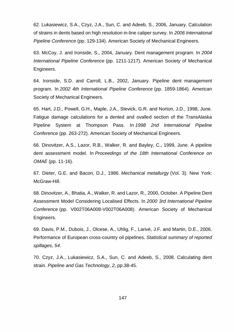
147

62. Lukasiewicz, S.A., Czyz, J.A., Sun, C. and Adeeb, S., 2006, January. Calculation

of strains in dents based on high resolution in-line caliper survey. In 2006 International

Pipeline Conference (pp. 129-134). American Society of Mechanical Engineers.

63. McCoy, J. and Ironside, S., 2004, January. Dent management program. In 2004


Engineers.

64. Ironside, S.D. and Carroll, L.B., 2002, January. Pipeline dent management

program. In 2002 4th International Pipeline Conference (pp. 1859-1864). American


65. Hart, J.D., Powell, G.H., Maple, J.A., Stevick, G.R. and Norton, J.D., 1998, June.

Fatigue damage calculations for a dented and ovalled section of the TransAlaska

Pipeline System at Thompson Pass. In 1998 2nd International Pipeline

Conference (pp. 263-272). American Society of Mechanical Engineers.

66. Dinovitzer, A.S., Lazor, R.B., Walker, R. and Bayley, C., 1999, June. A pipeline

dent assessment model. In Proceedings of the 18th International Conference on

OMAE (pp. 11-16).

67. Dieter, G.E. and Bacon, D.J., 1986. Mechanical metallurgy (Vol. 3). New York:

McGraw-Hill.

68. Dinovitzer, A., Bhatia, A., Walker, R. and Lazor, R., 2000, October. A Pipeline Dent

Assessment Model Considering Localised Effects. In 2000 3rd International Pipeline

Conference (pp. V002T06A008-V002T06A008). American Society of Mechanical

Engineers.

69. Davis, P.M., Dubois, J., Olcese, A., Uhlig, F., Larivé, J.F. and Martin, D.E., 2006.

Performance of European cross-country oil pipelines. Statistical summary of reported

spillages, 54.

70. Czyz, J.A., Lukasiewicz, S.A., Sun, C. and Adeeb, S., 2008. Calculating dent

strain. Pipeline and Gas Technology, 2, pp.38-45.

148

71. Browne, D. and Hicks, R., 2005. UKOPA Pipeline Fault Database, Pipeline Product

Loss Incidents (1962-2004). Fourth Report of the UKOPA Fault Database

Management Group prepared by Advantica for FDMG, UKOPA, UK.

72. ASTM, A.E., 2003. 1049–Standard practices for cycle counting in fatigue

analysis. West Conshohocken (PA).

73. Boiler, A.S.M.E. and Code, P.V., 2010. Section VIII Division 1. UG-126 Pressure

Relief Valves to UG-129 Marking, ASME International, New York, NY.

74. American Society of Mechanical Engineers, 1992. Liquid Transportation Systems

for Hydrocarbons, Liquid Petroleum Gas, Anhydrous Ammonia, and Alcohols: ASME

B31. 4. American Society of Mechanical Engineers.

75. Beuker, T. and Rahe, F., 2005. High-quality, smart pig dent inspection complies

with rules for gas, liquid lines. Pipeline & gas journal, 232(3), pp.40-44.

76. Clapham, L., Babbar, V. and Rubinshteyn, A., 2006, January. Understanding

Magnetic Flux Leakage Signals from Dents. In 2006 International Pipeline


77. EGIG Gas pipeline incidents: 6th Report of the European Gas Incident Data Group,

2005

78. Fowler, J. R. "Criteria for dent acceptability in offshore pipeline." In Offshore

Technology Conference. Offshore Technology Conference, 1993.

79. Johnston, D.C. and Hrncir, T.G., Using In-line Inspection to Address Deformations

Containing Near-neutral pH Stress Corrosion Cracking. 2002. Calgary, Alta., Canada:

American Society of Mechanical Engineers.

80. Lyons, D., 2002. Western European cross-country oil pipelines 30-year

performance statistics. CONCAWE.

81. Roovers, P., Bood, R., Galli, M., Marewski, U., Steiner, M. and Zaréa, M., 2000.

EPRG methods for assessing the tolerance and resistance of pipelines to external

damage. Pipeline technology, 2, pp.405-425.

149

82. Rosenfeld, M.J., Porter, P.C. and Cox, J.A., 1998, June. Strain estimation using

Vetco deformation tool data. In 1998 2nd International Pipeline Conference (pp. 389-

397). American Society of Mechanical Engineers

83. Rosenfeld, M.J., 2001. Proposed New Guidelines for ASME B31. 8 on Assessment

of Dents and Mechanical Damage: Topical Report. Gas Research Institute.

84. Rosenfeld, M.J., Pepper, J.W. and Leewis, K., 2002, January. Basis of the new

criteria in ASME B31. 8 for prioritization and repair of mechanical damage. In 2002 4th


Engineers.

85. Stevick, G.R., Hart, J.D. and Flanders, B., 1998, June. Fatigue curves for damage

calculations for a dented and ovalled section of the TransAlaska Pipeline System.

In 1998 2nd International Pipeline Conference (pp. 273-278). American Society of


86. Standard, A.P.I., 2001. 1160 Managing System Integrity for Hazardous Liquid

Pipelines. Firs Edition, November.

87. Hopkins, P., Jones, D.G. and Clyne, A., 1989, February. The significance of dents

and defects in transmission pipelines. In International Conference on Pipework

Engineering and Operations, London (pp. 137-145).

88. Eiber, R.J., 1981. The Effects of Dents on Failure Characteristics of Line Pipe.

American Gas Assn.

89. Eiber, R.J., 1979. Causes of pipeline failures probed. Oil and Gas J., 77(52), pp.80-

88.

90. Edward, D.C., 1988. A theoretical analysis of the formation of dents in pipeline

under station condition. British Gas. Engineering Research Station, Report, 4080.

91. Hopkins, P. and Corbin, P., 1988, September. A study of external damage of

pipelines. In Seventh american gas association symposium, Calgary, Alberta, Canada.

92. Hopkins, P., JONES, D. and Clyne, A., 1983. Recent studies of the significance of

mechanical damage in pipelines.

150

93. Wang, S.C., 2003. Artificial neural network. In Interdisciplinary computing in java

programming (pp. 81-100). Springer US.

94. Hepner, G. F. (1990). Artificial neural network classification using a minimal training

set. Comparison to conventional supervised classification. Photogrammetric

Engineering and Remote Sensing, 56(4), 469-473.

95. Hill, T., Marquez, L., O'Connor, M. and Remus, W., 1994. Artificial neural network

models for forecasting and decision making. International journal of forecasting, 10(1),

pp.5-15.

96. Dreiseitl, S. and Ohno-Machado, L., 2002. Logistic regression and artificial neural

network classification models: a methodology review. Journal of biomedical

informatics, 35(5), pp.352-359.

97. Elhewy, A.H., Mesbahi, E. and Pu, Y., 2006. Reliability analysis of structures using

neural network method. Probabilistic Engineering Mechanics, 21(1), pp.44-53.

98. Hopkins, P., Corder, I. and Corbin, P., 1992, June. The resistance of gas

transmission pipelines to mechanical damage. In International Conference on Pipeline

Reliability. (Vol. 2, p. 1992).

99. Hertz-Clemens, S., 2006, January. Experimental and Numerical Modelling of

Pipeline Denting. In 2006 International Pipeline Conference (pp. 171-179). American


100. Karamanos, S.A. and Andreadakis, K.P., 2006. Denting of internally pressurized

tubes under lateral loads. International Journal of Mechanical Sciences, 48(10),

pp.1080-1094.

101. Gresnigt, A.M., Karamanos, S.A. and Andreadakis, K.P., 2007. Lateral loading of

internally pressurized steel pipes. Journal of Pressure Vessel Technology, 129(4),

pp.630-638.

102. Hopkins, P., 1992, April. The application of fitness for purpose methods to defects

detected in offshore transmission pipelines. In Conference on welding and weld

performance in the process industry, London (pp. 27-28).

151

103. Gao, M., McNealy, R., Krishnamurthy, R. and Colquhoun, I., 2008, January.

Strain-based models for dent assessment: a review. In 2008 7th International Pipeline


104. FEA for all. 2013. What is an FEA solver? [Online]. Available at

http://feaforall.com/what-is-an-fea-solver/# [accessed 27 February 2017]

105. Fowler, J.R., Alexander, C.R., Kovach, P.J. and Connelly, L.M., 1994. Cyclic

Pressure Fatigue Life of Pipelines With Plain Dents, Dents With Gouges, and Dents

With Welds (No. AGA--94015627). American Gas Association, Inc., Arlington, VA

(United States); Stress Engineering Services, Inc., Houston, TX (United States).

106. ] Durowoju, M, Pu, Y, Benson, S & Race, J 2016, 'Fatigue assessment of pipeline

with plain dents under cyclic pressure loading using finite element method' pp. 1-10.

http://feaforall.com/what-is-an-fea-solver/

152

APPENDICES

Appendix A Spring Back Result

This section shows the table comparing the ratio of the initial dent depth (Hi) to the

spring back depth (Ho)for all pipe grades and diameter to thickness ratio (D/t). It shows

the comparison for both the dome and bar models. It also shows the other graphs

showing the effect of dent geometry, pipe geometry and pipe grade on the spring back

depth of dents as discussed in chapter 3.

DOME

d/D

(%)

D/t X46 X65 X80 X100

Hi

(%)

Ho

(%)

Hi/Ho Hi

(%)

Ho

(%)

Hi/Ho Hi (%) Ho

(%)

Hi/Ho Hi

(%)

Ho (%) Hi/Ho

2 18.6 2.78 1.90 1.46 2.78 1.60 1.74 3.71 2.30 1.61 4.02 2.30 1.75

25 2.78 1.80 1.55 3.40 2.00 1.70 4.64 1.60 2.90 4.33 2.30 1.88

32 3.40 2.20 1.55 3.40 1.80 1.89 4.02 2.20 1.83 4.02 1.80 2.23

40 3.09 1.70 1.82 3.40 1.60 2.12 4.33 2.20 1.97 4.64 2.00 2.32

50 3.09 1.80 1.72 3.71 1.60 2.32 4.94 2.30 2.15 4.94 1.90 2.60

62 3.09 1.80 1.72 5.25 2.50 2.10 5.25 2.20 2.39 5.87 2.10 2.80

80 3.09 2.20 1.40 5.56 2.30 2.42 6.80 2.60 2.61 5.25 1.30 4.04

96 2.78 1.90 1.46 5.87 2.10 2.80 6.80 2.60 2.61 6.49 1.60 4.06

5 18.6 5.87 4.90 1.20 6.18 4.50 1.37 6.49 5.00 1.30 8.03 5.80 1.39

25 7.11 5.70 1.25 6.49 4.60 1.41 7.11 5.40 1.32 8.34 5.70 1.46

32 5.56 4.30 1.29 6.80 4.60 1.48 7.11 5.00 1.42 8.03 5.00 1.61

40 7.11 5.30 1.34 7.11 4.60 1.55 8.03 5.10 1.58 8.96 5.30 1.69

50 6.49 4.40 1.47 7.42 4.70 1.58 8.96 5.50 1.63 8.96 4.90 1.83

62 7.11 5.00 1.42 8.34 4.80 1.74 10.20 5.80 1.76 10.20 5.00 2.04

80 7.73 4.60 1.68 10.51 5.50 1.91 11.43 5.50 2.08 11.43 4.70 2.43

96 9.27 4.90 1.89 11.74 5.60 2.10 12.98 5.60 2.32 11.43 3.90 2.93

7 18.6 8.03 7.20 1.12 8.65 7.00 1.24 9.89 7.80 1.27 10.51 7.90 1.33

25 8.03 6.90 1.16 8.96 7.30 1.23 9.89 7.50 1.32 10.51 7.50 1.40

32 7.42 6.00 1.24 8.96 6.60 1.36 9.58 7.20 1.33 10.51 7.10 1.48

153

40 8.65 6.70 1.29 9.58 6.90 1.39 10.82 7.40 1.46 11.43 7.30 1.57

50 9.58 7.00 1.37 9.89 6.60 1.50 11.74 7.70 1.52 11.74 6.90 1.70

62 10.20 6.90 1.48 11.12 6.90 1.61 12.98 7.70 1.69 13.29 7.10 1.87

80 11.43 7.00 1.63 12.67 7.00 1.81 14.21 7.50 1.90 14.52 6.50 2.23

96 12.36 7.00 1.77 15.14 7.60 1.99 16.69 7.70 2.17 16.07 6.20 2.59

10 18.6 10.51 9.60 1.09 10.82 9.10 1.19 11.74 10.20 1.15 13.60 10.80 1.26

25 10.82 9.50 1.14 12.36 10.10 1.22 13.29 10.80 1.23 14.52 11.00 1.32

32 10.82 9.10 1.19 12.67 9.90 1.28 13.60 10.50 1.29 14.21 10.20 1.39

40 12.67 10.30 1.23 12.67 9.60 1.32 14.52 10.50 1.38 14.21 9.60 1.48

50 12.36 9.40 1.31 13.91 9.90 1.40 15.76 10.80 1.46 15.14 9.50 1.59

62 13.60 9.70 1.40 15.76 10.50 1.50 17.30 10.60 1.63 16.69 9.40 1.78

80 15.14 9.80 1.55 17.00 10.00 1.70 18.85 10.60 1.78 18.85 9.10 2.07

96 16.38 9.90 1.65 19.78 10.80 1.83 21.94 11.30 1.94 23.18 10.10 2.29

BAR

d/D

(%)

D/t X46 X65 X80 X100

Hi

(%)

Ho

(%)

Hi/Ho Hi

(%)

Ho

(%)

Hi/Ho Hi (%) Ho

(%)

Hi/Ho Hi (%) Ho

(%)

Hi/Ho

2 18.6 3.40 1.80 1.89 4.02 1.90 2.11 4.33 1.90 2.28 4.33 1.50 2.88

25 4.02 1.90 2.11 4.64 1.90 2.44 4.94 1.80 2.75 5.25 1.70 3.09

32 4.64 2.10 2.21 5.25 1.90 2.76 5.87 2.00 2.94 6.18 1.80 3.43

40 5.25 2.10 2.50 5.87 1.90 3.09 6.49 1.90 3.42 7.42 2.00 3.71

50 5.56 1.90 2.93 6.49 1.80 3.61 7.42 1.90 3.90 8.34 1.90 4.39

62 6.80 2.20 3.09 7.73 1.90 4.07 8.96 2.10 4.27 9.27 1.80 5.15

80 7.11 1.60 4.44 9.58 2.10 4.56 10.82 2.10 5.15 10.82 1.60 6.76

96 8.34 1.80 4.64 11.74 2.40 4.89 12.36 1.90 6.51 12.05 1.50 8.03

5 18.6 6.80 5.00 1.36 7.11 4.70 1.51 8.03 5.30 1.52 8.03 4.60 1.75

25 7.11 4.80 1.48 7.73 4.70 1.64 8.65 5.00 1.73 9.58 5.00 1.92

32 8.03 5.10 1.58 8.65 4.80 1.80 9.58 5.00 1.92 11.12 5.30 2.10

40 8.96 5.30 1.69 9.58 4.80 2.00 10.51 4.90 2.14 12.36 5.30 2.33

50 9.27 4.80 1.93 10.82 4.70 2.30 12.67 5.40 2.35 14.21 5.10 2.79

154

62 10.82 5.10 2.12 12.98 5.30 2.45 15.14 6.00 2.52 14.83 4.50 3.30

80 11.74 4.60 2.55 14.83 5.30 2.80 17.30 5.60 3.09 17.30 4.60 3.76

96 13.60 5.10 2.67 16.07 5.20 3.09 18.85 5.90 3.19 18.85 4.40 4.28

7 18.6 8.96 7.10 1.26 8.96 6.50 1.38 10.20 7.30 1.40 10.82 7.10 1.52

25 9.89 7.40 1.34 9.89 6.70 1.48 10.82 7.00 1.55 12.05 7.20 1.67

32 10.51 7.40 1.42 10.20 6.20 1.64 11.74 6.90 1.70 13.29 7.10 1.87

40 11.12 7.30 1.52 12.05 7.00 1.72 13.60 7.50 1.81 14.52 7.00 2.07

50 11.12 6.30 1.77 13.60 7.20 1.89 15.45 7.80 1.98 17.00 7.00 2.43

62 13.29 7.30 1.82 14.52 6.80 2.14 16.38 7.30 2.24 17.30 6.30 2.75

80 13.91 6.30 2.21 17.30 7.70 2.25 17.92 6.70 2.67 19.78 6.30 3.14

96 15.45 6.80 2.27 18.85 7.50 2.51 21.01 7.60 2.76 23.48 7.30 3.22

10 18.6 12.36 10.50 1.18 12.36 9.80 1.26 12.36 9.50 1.30 13.91 10.00 1.39

25 12.05 9.60 1.26 13.60 10.2

0

1.33 13.60 9.70 1.40 15.45 10.20 1.51

32 13.29 10.10 1.32 14.83 10.6

0

1.40 14.83 9.90 1.50 17.00 10.40 1.63

40 14.52 10.60 1.37 13.91 8.70 1.60 16.69 10.60 1.57 18.23 10.20 1.79

50 16.07 11.40 1.41 15.45 9.10 1.70 18.23 11.00 1.66 20.39 9.70 2.10

62 15.45 9.60 1.61 17.30 9.80 1.77 20.09 11.20 1.79 21.63 10.30 2.10

80 17.92 10.50 1.71 19.78 10.0

0

1.98 22.25 10.60 2.10 23.18 9.00 2.58

96 19.78 11.00 1.80 22.87 11.0

0

2.08 25.96 11.40 2.28 27.81 10.50 2.65

155

A.1 Effect of pipe goemtery on spring back

A.1.1 Effect on circumferential dents

0.0

0.5

1.0

1.5

2.0

2.5

3.0

0 20 40 60 80 100 120

Hi/H

o

D/t

X65

2%

5%

7%

10%

0.0

0.5

1.0

1.5

2.0

2.5

3.0

0 20 40 60 80 100 120

Hi/H

o

D/t

X80

2%

5%

7%

10%

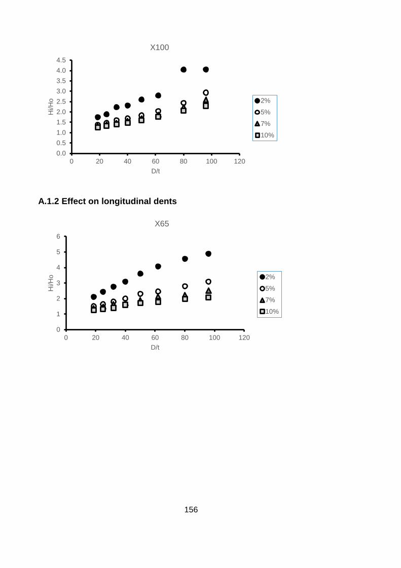
156

A.1.2 Effect on longitudinal dents

0.0

0.5

1.0

1.5

2.0

2.5

3.0

3.5

4.0

4.5

0 20 40 60 80 100 120

Hi/H

o

D/t

X100

2%

5%

7%

10%

0

1

2

3

4

5

6

0 20 40 60 80 100 120

Hi/H

o

D/t

X65

2%

5%

7%

10%

157

0

1

2

3

4

5

6

7

0 20 40 60 80 100 120

Hi/H

o

D/t

X80

2%

5%

7%

10%

0

1

2

3

4

5

6

7

8

9

0 20 40 60 80 100 120

Hi/H

o

D/t

X100

2%

5%

7%

10%

158

A.2 Effect of dent goemtery on spring back

0

1

2

3

4

5

6

7

8

9

10

0 20 40 60 80 100 120

Hi/H

o

D/t

X65

2% dome

2% bar

5% dome

5% bar

7% dome

7% bar

10% dome

10% bar

0.0

0.5

1.0

1.5

2.0

2.5

3.0

3.5

4.0

4.5

5.0

0 20 40 60 80 100 120

Hi/H

o

D/t

X46

2% dome

2% bar

5% dome

5% bar

7% dome

7% bar

10% dome

10% bar

159

A.3 Effect of pipe grades on spring back

A.3.1 Effect on circumferential dents

0

1

2

3

4

5

6

7

8

9

10

0 20 40 60 80 100 120

Hi/H

o

D/t

X80

2% dome

2% bar

5% dome

5% bar

7% dome

7% bar

10% dome

10% bar

0.0

0.5

1.0

1.5

2.0

2.5

3.0

3.5

4.0

4.5

0 20 40 60 80 100 120

Hi/H

o

D/t

2% dome

X46

X65

X80

X100

160

0.0

0.5

1.0

1.5

2.0

2.5

3.0

3.5

0 20 40 60 80 100 120

Hi/H

o

D/t

5% dome

X46

X65

X80

X100

0.0

0.5

1.0

1.5

2.0

2.5

3.0

0 20 40 60 80 100 120

Hi/H

o

D/t

7% dome

X46

X65

X80

X100

161

A.3.2 Effect on longitudinal dents

0

1

2

3

4

5

6

7

8

9

0 20 40 60 80 100 120

Hi/H

o

D/t

2% Bar

X46

X65

X80

X100

0.0

0.5

1.0

1.5

2.0

2.5

3.0

3.5

4.0

4.5

0 20 40 60 80 100 120

Hi/H

o

D/t

5% bar

X46

X65

X80

X100

162

0.0

0.5

1.0

1.5

2.0

2.5

3.0

3.5

0 20 40 60 80 100 120

Hi/H

o

D/t

7% bar

X46

X65

X80

X100

163

Appendix B Rerounding Result

This section shows the table comparing the ratio of the measured(spring back) dent

depth (Ho) to the reround depth (Hr)for all pipe grades and diameter to thickness ratio

(D/t). it shows the comparison for both the dome and bar models. It also shows the

other graphs showing the effect of dent geometry, pipe geometry and pipe grade on

the reround depth of dents as discussed in chapter 3.

Dome models

d/D

(%)

D/t X46 X65 X80 X100

Ho Hf Ho/Hf Ho Hf Ho/Hf Ho Hf Ho/Hf Ho Hf Ho/Hf

2 18.6 1.90 1.70 1.12 1.60 1.50 1.07 2.30 2.10 1.10 2.30 2.00 1.15

25 1.80 1.60 1.13 2.00 1.80 1.11 1.60 1.40 1.14 2.30 1.90 1.21

32 2.20 1.90 1.16 1.80 1.40 1.29 2.20 1.80 1.22 1.80 1.40 1.29

40 1.70 1.40 1.21 1.60 1.30 1.23 2.20 1.70 1.29 2.00 1.40 1.43

50 1.80 1.40 1.29 1.60 1.20 1.33 2.30 1.70 1.35 1.90 1.30 1.46

62 1.80 1.30 1.38 2.50 1.60 1.56 2.20 1.40 1.57 2.10 1.20 1.75

80 2.20 1.40 1.57 2.30 1.80 1.28 2.60 1.40 1.86 1.30 0.70 1.86

96 1.90 1.10 1.73 2.10 1.10 1.91 2.60 1.10 2.36 1.60 0.70 2.29

5 18.6 4.90 4.40 1.11 4.50 4.00 1.13 5.00 4.40 1.14 5.80 4.70 1.23

25 5.70 4.70 1.21 4.60 3.80 1.21 5.40 4.00 1.35 5.70 4.20 1.36

32 4.30 3.40 1.26 4.60 2.70 1.70 5.00 3.70 1.35 5.00 3.30 1.52

40 5.30 3.70 1.43 4.60 3.20 1.44 5.10 3.40 1.50 5.30 2.90 1.83

50 4.40 2.90 1.52 4.70 2.80 1.68 5.50 3.10 1.77 4.90 2.30 2.13

62 5.00 2.60 1.92 4.80 2.50 1.92 5.80 2.60 2.23 5.00 1.90 2.63

80 4.60 2.10 2.19 5.50 2.10 2.62 5.50 2.00 2.75 4.70 1.40 3.36

96 4.90 1.80 2.72 5.60 1.90 2.95 5.60 1.70 3.29 3.90 1.60 2.44

7 18.6 7.20 6.20 1.16 7.00 5.90 1.19 7.80 6.50 1.20 7.90 6.10 1.30

25 6.90 5.50 1.25 7.30 5.40 1.35 7.50 5.70 1.32 7.50 5.10 1.47

32 6.00 4.40 1.36 6.60 3.00 2.20 7.20 4.80 1.50 7.10 4.20 1.69

40 6.70 4.20 1.60 6.90 3.90 1.77 7.40 4.20 1.76 7.30 3.50 2.09

50 7.00 3.70 1.89 6.60 3.30 2.00 7.70 3.50 2.20 6.90 2.80 2.46

62 6.90 3.10 2.23 6.90 2.90 2.38 7.70 3.00 2.57 7.10 2.30 3.09

164

80 7.00 2.50 2.80 7.00 2.40 2.92 7.50 2.40 3.13 6.50 1.70 3.82

96 7.00 2.10 3.33 7.60 2.20 3.45 7.70 2.10 3.67 6.20 1.40 4.43

10 18.6 9.60 7.90 1.22 9.10 7.10 1.28 10.20 8.10 1.26 10.80 7.70 1.40

25 9.50 6.90 1.38 10.10 6.40 1.58 10.80 7.20 1.50 11.00 6.40 1.72

32 9.10 5.70 1.60 9.90 3.00 3.30 10.50 5.80 1.81 10.20 5.00 2.04

40 10.30 5.20 1.98 9.60 4.40 2.18 10.50 4.90 2.14 9.60 4.00 2.40

50 9.40 4.20 2.24 9.90 3.80 2.61 10.80 4.10 2.63 9.50 3.20 2.97

62 9.70 3.60 2.69 10.50 3.40 3.09 10.60 3.50 3.03 9.40 2.60 3.62

80 9.80 3.00 3.27 10.00 2.80 3.57 10.60 2.90 3.66 9.10 2.10 4.33

96 9.90 2.80 3.54 10.80 2.90 3.72 11.30 2.80 4.04 10.10 2.20 4.59

Bar models

d/D

(%)

D/t X46 X65 X80 X100

Ho Hf Ho/Hf Ho Hf Ho/Hf Ho Hf Ho/Hf Ho Hf Ho/Hf

2 18.6 1.80 1.40 1.29 1.90 1.50 1.27 1.90 1.50 1.27 1.50 1.10 1.36

25 1.90 1.50 1.27 1.90 1.40 1.36 1.80 1.30 1.38 1.70 1.10 1.55

32 2.10 1.40 1.50 1.90 1.30 1.46 2.00 1.40 1.43 1.80 1.10 1.64

40 2.10 1.40 1.50 1.90 1.20 1.58 1.90 1.20 1.58 2.00 1.10 1.82

50 1.90 1.20 1.58 1.80 1.10 1.64 1.90 1.10 1.73 1.90 1.10 1.73

62 2.20 1.30 1.69 1.90 1.10 1.73 2.10 1.20 1.75 1.80 0.90 2.00

80 1.60 0.90 1.78 2.10 1.10 1.91 2.10 1.20 1.75 1.60 0.80 2.00

96 1.80 1.00 1.80 2.40 1.40 1.71 1.90 1.10 1.73 1.50 0.80 1.88

5 18.6 5.00 3.60 1.39 4.70 3.30 1.42 5.30 3.50 1.51 4.60 2.90 1.59

25 4.80 3.10 1.55 4.70 2.90 1.62 5.00 2.90 1.72 5.00 2.70 1.85

32 5.10 2.80 1.82 4.80 2.70 1.78 5.00 2.70 1.85 5.30 2.60 2.04

40 5.30 2.80 1.89 4.80 2.50 1.92 4.90 2.50 1.96 5.30 2.50 2.12

50 4.80 2.50 1.92 4.70 2.50 1.88 5.40 2.60 2.08 5.10 2.30 2.22

62 5.10 2.50 2.04 5.30 2.60 2.04 6.00 2.60 2.31 4.50 2.10 2.14

80 4.60 2.30 2.00 5.30 2.40 2.21 5.60 2.40 2.33 4.60 1.90 2.42

96 5.10 2.40 2.13 5.20 2.20 2.36 5.90 2.30 2.57 4.40 1.80 2.44

165

7 18.6 7.10 4.60 1.54 6.50 4.10 1.59 7.30 4.30 1.70 7.10 4.00 1.78

25 7.40 4.10 1.80 6.70 3.60 1.86 7.00 3.70 1.89 7.20 3.50 2.06

32 7.40 3.60 2.06 6.20 3.20 1.94 6.90 3.30 2.09 7.10 3.20 2.22

40 7.30 3.30 2.21 7.00 3.20 2.19 7.50 3.30 2.27 7.00 2.90 2.41

50 6.30 3.00 2.10 7.20 3.10 2.32 7.80 3.10 2.52 7.00 2.80 2.50

62 7.30 3.00 2.43 6.80 2.90 2.34 7.30 2.90 2.52 6.30 2.50 2.52

80 6.30 2.80 2.25 7.70 2.90 2.66 6.70 2.60 2.58 6.30 2.40 2.63

96 6.80 2.80 2.43 7.50 2.90 2.59 7.60 2.80 2.71 7.30 2.50 2.92

10 18.6 10.50 5.90 1.78 9.80 5.20 1.88 9.50 5.00 1.90 10.00 5.60 1.79

25 9.60 4.70 2.04 10.20 4.60 2.22 9.70 4.40 2.20 10.20 4.30 2.37

32 10.10 4.20 2.40 10.60 4.10 2.59 9.90 3.90 2.54 10.40 3.80 2.74

40 10.60 3.90 2.72 8.70 3.50 2.49 10.60 3.70 2.86 10.20 3.40 3.00

50 11.40 3.70 3.08 9.10 3.30 2.76 11.00 3.50 3.14 9.70 3.10 3.13

62 9.60 3.30 2.91 9.80 3.30 2.97 11.20 3.50 3.20 10.30 3.20 3.22

80 10.50 3.50 3.00 10.00 3.50 2.86 10.60 3.60 2.94 9.00 2.90 3.10

96 11.00 3.60 3.06 11.00 3.80 2.89 11.40 3.80 3.00 10.50 3.30 3.18

B.1 Effect of pipe goemtery on rerounding

B.1.1 Effect on circumferential dents

0.0

0.5

1.0

1.5

2.0

2.5

3.0

3.5

4.0

0 20 40 60 80 100 120

Ho

/Hr

D/t

X65

2%

5%

7%

10%

166

0.0

0.5

1.0

1.5

2.0

2.5

3.0

3.5

4.0

4.5

0 20 40 60 80 100 120

Ho

/Hr

D/t

X80

2%

5%

7%

10%

0.0

0.5

1.0

1.5

2.0

2.5

3.0

3.5

4.0

4.5

5.0

0 20 40 60 80 100 120

Ho

/Hr

D/t

X100

2%

5%

7%

10%

167

B.1.2 Effect on longitudinal dents

0.0

0.5

1.0

1.5

2.0

2.5

3.0

3.5

0 20 40 60 80 100 120

Ho

/Hr

D/t

X65 Bar

2%

5%

7%

10%

0.0

0.5

1.0

1.5

2.0

2.5

3.0

3.5

0 20 40 60 80 100 120

Ho

/Hr

D/t

X80 Bar

2%

5%

7%

10%

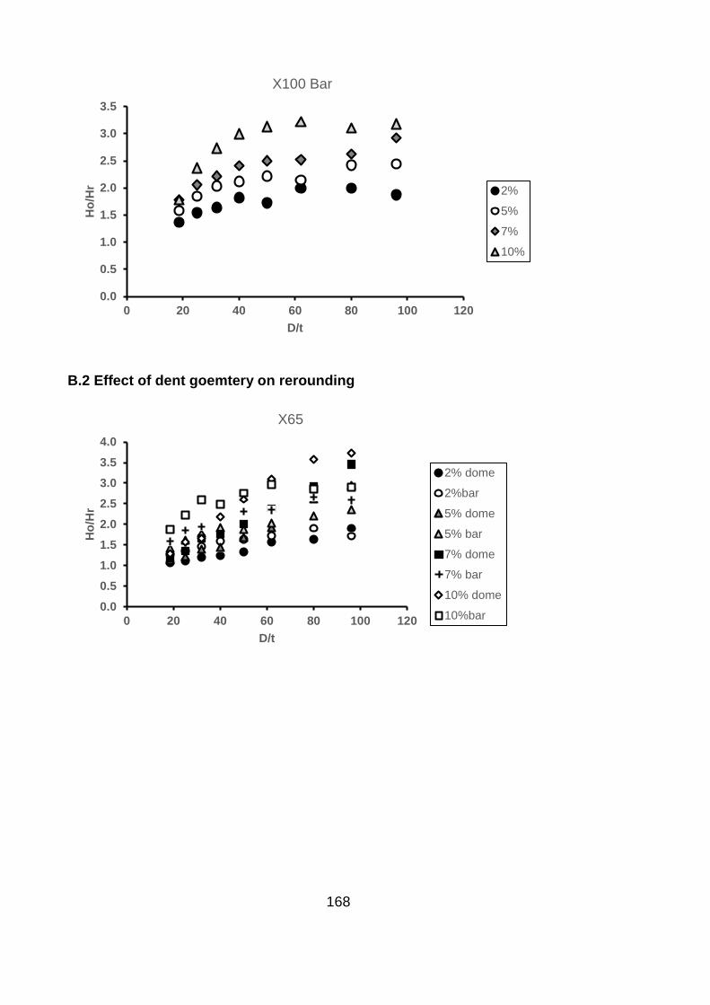
168

B.2 Effect of dent goemtery on rerounding

0.0

0.5

1.0

1.5

2.0

2.5

3.0

3.5

0 20 40 60 80 100 120

Ho

/Hr

D/t

X100 Bar

2%

5%

7%

10%

0.0

0.5

1.0

1.5

2.0

2.5

3.0

3.5

4.0

0 20 40 60 80 100 120

Ho

/Hr

D/t

X65

2% dome

2%bar

5% dome

5% bar

7% dome

7% bar

10% dome

10%bar

169

0.0

0.5

1.0

1.5

2.0

2.5

3.0

3.5

4.0

4.5

0 20 40 60 80 100 120

Ho

/Hr

D/t

X80

2% dome

2% bar

5% dome

5% bar

7% dome

7% bar

10% dome

10% bar

0.0

0.5

1.0

1.5

2.0

2.5

3.0

3.5

4.0

4.5

5.0

0 20 40 60 80 100 120

Ho

/Hr

D/t

X100

2% dome

2% bar

5% dome

5% bar

7% dome

7% bar

10% dome

10% bar

170

B.3 Effect of pipe grade on rerounding

B.3.1 Effect on circumferential dents

0.0

0.5

1.0

1.5

2.0

2.5

0 20 40 60 80 100 120

Ho

/Hr

D/t

2% dome

X46

X65

X80

x100

0.0

0.5

1.0

1.5

2.0

2.5

3.0

3.5

4.0

0 20 40 60 80 100 120

Ho

/Hr

D/t

5% dome

X46

X65

X80

X100

171

B.3.2 Effect on longitudinal dents

0.0

0.5

1.0

1.5

2.0

2.5

3.0

3.5

4.0

4.5

5.0

0 20 40 60 80 100 120

Ho

/Hr

D/t

7% dome

X46

X65

X80

X100

0.0

0.5

1.0

1.5

2.0

2.5

0 20 40 60 80 100 120

Ho

/Hr

D/t

2% bar

X46

X65

X80

X100

172

0.0

0.5

1.0

1.5

2.0

2.5

3.0

0 20 40 60 80 100 120

Ho

/Hr

D/t

5% bar

X46

X65

X80

X100

0.0

0.5

1.0

1.5

2.0

2.5

3.0

3.5

0 20 40 60 80 100 120

Ho

/Hr

D/t

7% bar

X46

X65

X80

X100

173

Appendix C SCF Results

This section shows other graphs illustrating the effects of pipe geometry and pipe

grades on the SCF in dented pipelines as discussed in chapter 4.it shows the results

for different dent depths at different pressure ranges for both the dome and bar dent.

C.1 Effect of pipe goemtery and pipe grade on SCF

C.1.1 Effect on dome dents

0

20

40

60

80

100

120

0 20 40 60 80 100 120

∆σ

/∆p

D/t

5% d/D,50smys

X46

X65

X80

X100

0

20

40

60

80

100

120

0 20 40 60 80 100 120

∆σ

/∆p

D/t

5% d/D,72smys

X46

X65

X80

X100

174

0

20

40

60

80

100

120

0 20 40 60 80 100 120

∆σ

/∆p

D/t

7%d/D,50smys

X46

X65

X80

X100

0

20

40

60

80

100

120

0 20 40 60 80 100 120

∆σ

/∆p

D/t

7% d/D,72smsys

X46

X65

X80

X100

175

0

20

40

60

80

100

120

0 20 40 60 80 100 120

∆σ

/∆p

D/t

10% d/D, 50smys

X46

X65

X80

X100

0

20

40

60

80

100

120

0 20 40 60 80 100 120

∆σ

/∆p

D/t

10% d/D, 72smsys

X46

X65

X80

X100

176

C.1.2 Effect on bar dents

0

20

40

60

80

100

120

0 20 40 60 80 100 120

∆σ

/∆p

D/t

5%,d/D, 50smys

X46

X65

X80

X100

0

20

40

60

80

100

120

0 20 40 60 80 100 120

∆σ

/∆p

D/t

5% d/D, 72smys

X46

X65

X80

X100

177

0

20

40

60

80

100

120

0 20 40 60 80 100 120

∆σ

/∆p

D/t

7% d/D, 50smys

X46

X65

X80

X100

0

20

40

60

80

100

120

0 20 40 60 80 100 120

∆σ

/∆p

D/t

7% d/D, 72smys

X46

X65

X80

X100

178

0

20

40

60

80

100

120

0 20 40 60 80 100 120

∆σ

/∆p

D/t

10% d/D, 50smsys

X46

X65

X80

X100

0

20

40

60

80

100

120

0 20 40 60 80 100 120

∆σ

/∆p

D/t

10% d/D, 72smys

X46

X65

X80

X100

179

Appendix D Strain Results

This section shows the other graphs illustrating the effects of pipe geometry and pipe

grades on the maximum strain for both the dome and bar dents as discussed in chapter

5. It compares the effect on different dent depths.

D.1 Effect of pipe goemtery on Strain

D.1.1 Effect on dome dents

0.00

0.02

0.04

0.06

0.08

0.10

0.12

0.14

0 20 40 60 80 100 120

max s

train

D/t

Effect of pipe geometry for a 2% dome X46 pipe grade


longitudinal strain

total strain

0.00

0.02

0.04

0.06

0.08

0.10

0.12

0.14

0.16

0.18

0.20

0 20 40 60 80 100 120

ma

x s

train

D/t



longitudinal strain

total strain

180

D.1.2 Effect on bar dents

0.00

0.05

0.10

0.15

0.20

0.25

0 20 40 60 80 100 120

max s

train

D/t



longitudinal strain

total strain

0.00

0.02

0.04

0.06

0.08

0.10

0.12

0.14

0 20 40 60 80 100 120

max s

train

D/t

Effect of pipe geometry for a 2% bar X46 grade


longitudinal strain

total strain

181

0.00

0.05

0.10

0.15

0.20

0.25

0.30

0 20 40 60 80 100 120

ma

x s

train

D/t



longitudinal strain

total strain

0.00

0.05

0.10

0.15

0.20

0.25

0.30

0.35

0 20 40 60 80 100 120

ma

x s

train

D/t



longitudinal strain

total strain

182

D.2 Effect of pipe grade on Strain

D.2.1 Effect on dome dents

0.00

0.02

0.04

0.06

0.08

0.10

0.12

0.14

0 20 40 60 80 100 120

max s

train

D/t

Effect of pipe grade for 2% dome

X46

X65

X80

X100

0.00

0.05

0.10

0.15

0.20

0.25

0 20 40 60 80 100 120

max s

train

D/t


X46

X65

X80

X100

183

D.2.2 Effect on bar dents

0.00

0.05

0.10

0.15

0.20

0.25

0 20 40 60 80 100 120

ma

x s

train

D/t


X46

X65

X80

X100

0.00

0.02

0.04

0.06

0.08

0.10

0.12

0.14

0.16

0 20 40 60 80 100 120

ma

x s

train

D/t


X46

X65

X80

X100

184

0.00

0.05

0.10

0.15

0.20

0.25

0.30

0 20 40 60 80 100 120

max s

train

D/t


X46

X65

X80

X100

0.00

0.05

0.10

0.15

0.20

0.25

0.30

0.35

0 20 40 60 80 100 120

max s

train

D/t


X46

X65

X80

X100

185

Appendix E Ansys mechanical APDL log file

This section shows the Ansys parametric design language (APDL) used for modelling

both the dome and the bar dents. With APDL, several models can be created by

changing the parameters highlighted in red and copying and pasting in the command

window. The APDL file also contains comments highlighting the purpose of a particular

command in order to help a first time user understand the command. The comments

section begins with an exclamation mark(!) followed by the word comment and this is

not part of the codes.it should be noted that sentences in italics are not part of the

codes and is only used to describe a particular command or variable

E.1 Apdl file for a dome dent

! comments: setting preferences- the below codes helps select static structural analysis by disabling every other analysis settings, static structural is set as 1 and all other analysis set as 0 as shown by the red highlights /NOPR KEYW,PR_SET,1 KEYW,PR_STRUC,1 KEYW,PR_THERM,0 KEYW,PR_FLUID,0 KEYW,PR_ELMAG,0 KEYW,MAGNOD,0 KEYW,MAGEDG,0 KEYW,MAGHFE,0 KEYW,MAGELC,0 KEYW,PR_MULTI,0 /GO !* /COM, /COM,Preferences for GUI filtering have been set to display: /COM, Structural !* ! comments: Selecting elements; This is the section where elements are selected /PREP7 !* ET,1,SOLID186 !* ET,2,TARGE170 !* ET,3,CONTA174 !* ! comments: defining real constant; for older version of ansys, the real constants of element needs to be defined, however, some of the new elements do not require real constants R,1, , , !* R,2,,,, ,,

186

RMORE,,,, ,, RMORE,,,, ,, RMORE,,,, ,, RMORE,,,,,, RMORE,,,,, !* !* ! comments: defining material properties; here the material model and properties are defined

MPTEMP,,,,,,,, MPTEMP,1,0 MPDATA,EX,1,,210000 ! Young’s modulus MPDATA,PRXY,1,,0.3 ! Poisson ratio TB,KINH,1,1,11,0 TBTEMP,0 TBPT,,0.002211904762,464.5 ! stress-strain data

TBPT,,0.05,560 TBPT,,0.1,625 TBPT,,0.2,690 TBPT,,0.3,750 TBPT,,0.4,775 TBPT,,0.5,800 TBPT,,0.6,825 TBPT,,0.8,860 TBPT,,0.9,880 TBPT,,1,900 ! comments: defining key points; this is the point where the geometry creation starts, four key points are created with the first key point starting from the origin as indicated as 0,0,0. The second key point shows the thickness of the pipe. The 3rd and 4th key point completes the quarter symmetry of the pipe K,1,0,0,0, K,2,0,17.399,0, K,3,0,306.221,0, K,4,0,323.62,0, KPLOT ! comments: key points 5,6 and 7 defines the radius of the outer and inner wall of the pipe. These points are created in order to be able to create arcs joining the points K,5,161.81,161.81,0, K,6,144.411,161.81,0, K,7,0,161.81,0, ! comments: Creating lines between key points

LSTR, 1, 2 LSTR, 3, 4 !* ! comments: creating arcs between key points LARC,4,5,7,161.81, ! radius of outer wall

!* LARC,1,5,7,161.81, !* LARC,3,6,7,144.411, ! radius of inner wall

!* LARC,6,2,7,144.411, LSTR, 6, 5 LPLOT /PNUM,KP,0 /PNUM,LINE,1 /PNUM,AREA,0 /PNUM,VOLU,0

187

/PNUM,NODE,0 /PNUM,TABN,0 /PNUM,SVAL,0 /NUMBER,0 !* /PNUM,ELEM,0 /REPLOT !* ! comments :creating areas between lines al,2,3,5,7 al,1,4,6,7 ! comments: Extruding areas; the areas are extruded 3 times to create the 3 different volumes. Both the upper and lower half needs to be extruded VOFFST,1,328.605, , VOFFST,3,200, , VOFFST,8,721.395, , VOFFST,2,328.605, , VOFFST,18,200, , VOFFST,23,721.395, , ! comments: Creating key point to draw dome indenter K,100,0,323.62,, ! start of the key point which is at the top of the pipe in order to simulate contact K,101,0,433.355,, K,102,109.535,433.355, ! comments: creating lines between key points LSTR, 100, 101 LSTR, 101, 102 !* ! comments: creating arc between key points

LARC,102,100,101,109.535, ! radius of the dome LPLOT al,56,57,58 FLST,2,1,5,ORDE,1 FITEM,2,33 FLST,8,2,3 FITEM,8,101 FITEM,8,100 VROTAT,P51X, , , , , ,P51X, ,360,4, FLST,2,3,6,ORDE,2 FITEM,2,7 FITEM,2,-9 ! comments: deleting unwanted volume VDELE,P51X, , ,1 APLOT LPLOT VPLOT

188

! comments: defining element size for indenter

ESIZE,10,0, ! element size MSHAPE,0,3D MSHKEY,1 !* CM,_Y,VOLU VSEL, , , , 10 CM,_Y1,VOLU CHKMSH,'VOLU' CMSEL,S,_Y !* ! comments: meshing the indenter VMESH,_Y1 !* CMDELE,_Y CMDELE,_Y1 CMDELE,_Y2 !* VPLOT ! comments: adding the three volumes in the pipe vadd,3,6 vadd,2,5 vadd,1,4 VPLOT LPLOT FLST,5,4,4,ORDE,4 FITEM,5,12 FITEM,5,-13 FITEM,5,36 FITEM,5,-37 CM,_Y,LINE LSEL, , , ,P51X CM,_Y1,LINE CMSEL,,_Y !* FLST,5,4,4,ORDE,4 FITEM,5,12 FITEM,5,-13 FITEM,5,36 FITEM,5,-37 CM,_Y,LINE LSEL, , , ,P51X CM,_Y1,LINE CMSEL,,_Y !* ! comments: line sizing; this is the point where the lines are divided to create the number of elements and bias

LESIZE,_Y1, , ,80,3, , , ,1 ! 80 is the number of division and 3 is the bias factor !* FLST,5,4,4,ORDE,4 FITEM,5,3 FITEM,5,5 FITEM,5,9 FITEM,5,11 CM,_Y,LINE LSEL, , , ,P51X CM,_Y1,LINE CMSEL,,_Y

189

!* LESIZE,_Y1, , ,30, , , , ,1 !* FLST,5,4,4,ORDE,4 FITEM,5,4 FITEM,5,6 FITEM,5,49 FITEM,5,-50 CM,_Y,LINE LSEL, , , ,P51X CM,_Y1,LINE CMSEL,,_Y !* LESIZE,_Y1, , ,20, , , , ,1 !* FLST,5,4,4,ORDE,4 FITEM,5,1 FITEM,5,-2 FITEM,5,8 FITEM,5,32 CM,_Y,LINE LSEL, , , ,P51X CM,_Y1,LINE CMSEL,,_Y !* LESIZE,_Y1, , ,6, , , , ,1 !* CM,_Y,VOLU VSEL, , , , 2 CM,_Y1,VOLU CHKMSH,'VOLU' CMSEL,S,_Y !* ! comments: meshing the main volume of the pipe VSWEEP,_Y1 !* CMDELE,_Y CMDELE,_Y1 CMDELE,_Y2 !* VPLOT ! comment: defining element size for the other volumes ESIZE,60,0, ! element size VPLOT FLST,5,2,6,ORDE,2 FITEM,5,3 FITEM,5,7 CM,_Y,VOLU VSEL, , , ,P51X CM,_Y1,VOLU CHKMSH,'VOLU' CMSEL,S,_Y !* ! comments: meshing other volumes VSWEEP,_Y1 !* CMDELE,_Y CMDELE,_Y1 CMDELE,_Y2 !*

190

! comments: selecting the target area ASEL,S, , , 44 APLOT /REPLO NSLA,S,1 NPLOT ! comments: selecting target nodes from the area FLST,5,784,1,ORDE,5 FITEM,5,2 FITEM,5,38 FITEM,5,-73 FITEM,5,785 FITEM,5,-1531 NSEL,R, , ,P51X CM,target,NODE CMSEL,A,target /MREP,EPLOT ALLSEL,ALL VPLOT ! comments: selecting contact nodes

NSEL,S,LOC,X,0,161.81 ! location on the x axis NPLOT NSEL,R,LOC,Y,306.221,323.62 ! location on the y axis

NPLOT NSEL,R,LOC,Z,0,-140 ! location on the Z axis NPLOT ! comments: automatically selected nodes based on the location selected( no need to copy and paste as it automatically generated using the above commands) FLST,5,7547,1,ORDE,897 FITEM,5,785 FITEM,5,14499 FITEM,5,-14543 FITEM,5,14613 FITEM,5,-14702 FITEM,5,14737 FITEM,5,-14781 FITEM,5,14851 FITEM,5,-14940 FITEM,5,14975 FITEM,5,-15019 FITEM,5,15089 FITEM,5,-15178 FITEM,5,15213 FITEM,5,-15257 FITEM,5,15327 FITEM,5,-15416 FITEM,5,15451 FITEM,5,-15495 FITEM,5,15565 FITEM,5,-15654 FITEM,5,15689 FITEM,5,-15891 FITEM,5,15899 FITEM,5,-15905 FITEM,5,16288 FITEM,5,-16295 FITEM,5,16339 FITEM,5,-16354

191

FITEM,5,16377 FITEM,5,-16383 FITEM,5,16429 FITEM,5,-16442 FITEM,5,16466 FITEM,5,-16471 FITEM,5,16519 FITEM,5,-16530 FITEM,5,16555 FITEM,5,-16559 FITEM,5,16609 FITEM,5,-16618 FITEM,5,16644 FITEM,5,-16647 FITEM,5,16700 FITEM,5,-16706 FITEM,5,16734 FITEM,5,-16735 FITEM,5,16765 FITEM,5,-16781 FITEM,5,17349 FITEM,5,-17356 FITEM,5,17399 FITEM,5,-17415 FITEM,5,17437 FITEM,5,-17444 FITEM,5,17487 FITEM,5,-17503 FITEM,5,17525 FITEM,5,-17532 FITEM,5,17575 FITEM,5,-17591 FITEM,5,17613 FITEM,5,-17620 FITEM,5,17663 FITEM,5,-17679 FITEM,5,17701 FITEM,5,-17708 FITEM,5,17751 FITEM,5,-17767 FITEM,5,17789 FITEM,5,-17796 FITEM,5,17839 FITEM,5,-17855 FITEM,5,17877 FITEM,5,-17884 FITEM,5,17927 FITEM,5,-17943 FITEM,5,17965 FITEM,5,-17972 FITEM,5,18015 FITEM,5,-18031 FITEM,5,18053 FITEM,5,-18060 FITEM,5,18103 FITEM,5,-18119 FITEM,5,18141 FITEM,5,-18148 FITEM,5,18191 FITEM,5,-18207 FITEM,5,18229 FITEM,5,-18236 FITEM,5,18279 FITEM,5,-18295 FITEM,5,18317 FITEM,5,-18324

192


193


194


195


196


197


198


199


200


201


202


203


204

FITEM,5,54765 FITEM,5,-54766 FITEM,5,54776 FITEM,5,-54777 FITEM,5,54787 FITEM,5,-54788 FITEM,5,54798 FITEM,5,-54799 FITEM,5,54809 FITEM,5,-54810 NSEL,R, , ,P51X CM,contact,NODE CMSEL,A,contact /MREP,EPLOT ALLSEL,ALL VPLOT ! comments: creating contact pair /COM, CONTACT PAIR CREATION - START CM,_NODECM,NODE CM,_ELEMCM,ELEM CM,_KPCM,KP CM,_LINECM,LINE CM,_AREACM,AREA CM,_VOLUCM,VOLU /GSAV,cwz,gsav,,temp MP,MU,1,0.2 ! coefficient of friction MAT,1 MP,EMIS,1,7.88860905221e-031 R,3 REAL,3 ET,4,170 ET,5,175 R,3,,,1.0,0.1,0, RMORE,,,1.0E20,0.0,1.0, RMORE,0.0,0,1.0,,1.0,0.5 RMORE,0,1.0,1.0,0.0,,1.0 RMORE,10.0 KEYOPT,5,4,0 KEYOPT,5,5,3 KEYOPT,5,7,0 KEYOPT,5,8,0 KEYOPT,5,9,1 KEYOPT,5,10,2 KEYOPT,5,11,0 KEYOPT,5,12,0 KEYOPT,5,2,0 KEYOPT,4,5,0 ! Generate the target surface NSEL,S,,,TARGET CM,_TARGET,NODE TYPE,4 ESLN,S,0 ESURF CMSEL,S,_ELEMCM ! Generate the contact surface NSEL,S,,,CONTACT CM,_CONTACT,NODE TYPE,5 ESLN,S,0 ESURF ALLSEL ESEL,ALL ESEL,S,TYPE,,4 ESEL,A,TYPE,,5

205

ESEL,R,REAL,,3 /PSYMB,ESYS,1 /PNUM,TYPE,1 /NUM,1 EPLOT ESEL,ALL ESEL,S,TYPE,,4 ESEL,A,TYPE,,5 ESEL,R,REAL,,3 CMSEL,A,_NODECM CMDEL,_NODECM CMSEL,A,_ELEMCM CMDEL,_ELEMCM CMSEL,S,_KPCM CMDEL,_KPCM CMSEL,S,_LINECM CMDEL,_LINECM CMSEL,S,_AREACM CMDEL,_AREACM CMSEL,S,_VOLUCM CMDEL,_VOLUCM /GRES,cwz,gsav CMDEL,_TARGET CMDEL,_CONTACT /COM, CONTACT PAIR CREATION - END /MREP,EPLOT ALLSEL,ALL /REPLOT VPLOT ! comments: defining major volumes and area for viewing results CM,indenter,VOLU CMSEL,A,indenter CMDELE,indenter VSEL,R, , , 10 CM,indenter,VOLU CMSEL,A,indenter VSEL,R, , , 2 CM,keyvolume,VOLU CMSEL,A,keyvolume ASEL,R, , , 5 CM,extarea,AREA CMSEL,A,extarea ASEL,R, , , 7 CM,intarea,AREA CMSEL,A,intarea /MREP,EPLOT ALLSEL,ALL VPLOT FINISH CMDELE,INTAREA CMDELE,KEYVOLUME VSEL,R, , , 2 CM,keyvolume,VOLU CMSEL,A,keyvolume ASEL,R, , , 7 CM,intarea,AREA CMSEL,A,intarea /MREP,EPLOT ALLSEL,ALL VPLOT /MREP,EPLOT ALLSEL,ALL VPLOT

206

! comments: Applying boundary conditions and loading

/SOLU FLST,2,10,5,ORDE,10 FITEM,2,1 FITEM,2,-2 FITEM,2,4 FITEM,2,9 FITEM,2,14 FITEM,2,19 FITEM,2,24 FITEM,2,29 FITEM,2,33 FITEM,2,42 DA,P51X,SYMM FLST,2,3,4,ORDE,3 FITEM,2,36 FITEM,2,44 FITEM,2,52 !* /GO DL,P51X, ,UY,0 /VIEW, 1, -0.413493917123 , 0.194139313190E-01, -0.910299884529 /ANG, 1, -4.24338859683 /REPLO FLST,2,2,5,ORDE,2 FITEM,2,13 FITEM,2,35 !* /GO DA,P51X,UZ,0 FLST,2,1,5,ORDE,1 FITEM,2,44 !* /GO DA,P51X,UX,0 FLST,2,1,5,ORDE,1 FITEM,2,44 !* /GO DA,P51X,UZ,0 FLST,2,1,5,ORDE,1 FITEM,2,44 !* /GO DA,P51X,UY,-9 ! initial dent depth before removal of indenter LSWRITE,1, ! Defining load steps FLST,2,1,5,ORDE,1 FITEM,2,44 !* /GO DA,P51X,ALL,0 ! removing indenter LSWRITE,2, FLST,2,6,5,ORDE,6 FITEM,2,7 FITEM,2,12 FITEM,2,17 FITEM,2,23 FITEM,2,30 FITEM,2,37 /GO !* SFA,P51X,1,PRES,27.6 ! applying pressure LSWRITE,3, FLST,2,6,5,ORDE,6 FITEM,2,7

207

FITEM,2,12 FITEM,2,17 FITEM,2,23 FITEM,2,30 FITEM,2,37 /GO !* SFA,P51X,1,PRES,34.6 LSWRITE,4, FLST,2,6,5,ORDE,6 FITEM,2,7 FITEM,2,12 FITEM,2,17 FITEM,2,23 FITEM,2,30 FITEM,2,37 /GO !* SFA,P51X,1,PRES,24.1 LSWRITE,5, FLST,2,6,5,ORDE,6 FITEM,2,7 FITEM,2,12 FITEM,2,17 FITEM,2,23 FITEM,2,30 FITEM,2,37 /GO !* SFA,P51X,1,PRES,0 LSWRITE,6, FLST,2,6,5,ORDE,6 FITEM,2,7 FITEM,2,12 FITEM,2,17 FITEM,2,23 FITEM,2,30 FITEM,2,37 /GO !* SFA,P51X,1,PRES,24.1 LSWRITE,7, FLST,2,6,5,ORDE,6 FITEM,2,7 FITEM,2,12 FITEM,2,17 FITEM,2,23 FITEM,2,30 FITEM,2,37 /GO !* SFA,P51X,1,PRES,34.6 LSWRITE,8, FLST,2,6,5,ORDE,6 FITEM,2,7 FITEM,2,12 FITEM,2,17 FITEM,2,23 FITEM,2,30 FITEM,2,37 /GO !* SFA,P51X,1,PRES,0 LSWRITE,9, FLST,2,6,5,ORDE,6 FITEM,2,7

208

FITEM,2,12 FITEM,2,17 FITEM,2,23 FITEM,2,30 FITEM,2,37 /GO !* SFA,P51X,1,PRES,24.1 LSWRITE,10, FLST,2,6,5,ORDE,6 FITEM,2,7 FITEM,2,12 FITEM,2,17 FITEM,2,23 FITEM,2,30 FITEM,2,37 /GO !* SFA,P51X,1,PRES,34.6 LSWRITE,11, FLST,2,6,5,ORDE,6 FITEM,2,7 FITEM,2,12 FITEM,2,17 FITEM,2,23 FITEM,2,30 FITEM,2,37 /GO !* SFA,P51X,1,PRES,0 ! removing pressure LSWRITE,12, !* ! comments: defining non-linear settings ANTYPE,0 NLGEOM,1 NSUBST,100,1000,10 ! defining sub-steps

OUTRES,ERASE OUTRES,ALL,1 AUTOTS,1 LNSRCH,1 TIME,1 /nerr,10000,10000,off ! comments: Solving by load steps

LSSOLVE,1,12,1, FINISH ! comments: post processing phase

/POST1 /SHOW,WIN32C SET,FIRST /PLOPTS,INFO,3 /CONTOUR,ALL,18 /PNUM,MAT,1 /NUMBER,1 /REPLOT,RESIZE SET,,,,,,,15 PLESOL,S,1 SET,,,,,,,30 PLESOL,S,1 SET,,,,,,,180 PLESOL,S,1

209

SET,,,,,,,165 PLESOL,S,1 SET,,,,,,,150 PLESOL,S,1 PLNSOL,S,1 SET,,,,,,,165 PLNSOL,S,1 ! /UIS,ABORT,1 /SHOW,WIN32 /REPLOT,RESIZE FINISH ! /EXIT,ALL

E.2 Apdl file for a bar dent ! comments: setting preferences- the below codes helps select static structural analysis by disabling every other analysis settings, static structural is set as 1 and all other analysis set as 0 as shown by the red highlights /NOPR KEYW,PR_SET,1 KEYW,PR_STRUC,1 KEYW,PR_THERM,0 KEYW,PR_FLUID,0 KEYW,PR_ELMAG,0 KEYW,MAGNOD,0 KEYW,MAGEDG,0 KEYW,MAGHFE,0 KEYW,MAGELC,0 KEYW,PR_MULTI,0 /GO !* /COM, /COM,Preferences for GUI filtering have been set to display: /COM, Structural !* ! comments: Selecting elements; This is the section where elements are selected /PREP7 !* ET,1,SOLID186 !* ET,2,TARGE170 !* ET,3,CONTA174 !* ! comments: defining real constant; for older version of ansys, the real constants of element needs to be defined, however, some of the new elements do not require real constants R,1, , , !* R,2,,,, ,, RMORE,,,, ,, RMORE,,,, ,, RMORE,,,, ,, RMORE,,,,,, RMORE,,,,, !* ! comments: defining material properties; here the material model and properties are defined

210

MPTEMP,,,,,,,, MPTEMP,1,0 MPDATA,EX,1,,210000 ! Young’s modulus MPDATA,PRXY,1,,0.3 ! Poisson ratio

/CWD,'D:\ansys' !* TB,KINH,1,1,8,0 TBTEMP,0 TBPT,,0.0015,315 ! stress-strain data TBPT,,0.003,337 TBPT,,0.012,374 TBPT,,0.02,386 TBPT,,0.05,418 TBPT,,0.07,430 TBPT,,0.09,437 TBPT,,0.135,443 ! comments: defining key points; this is the point where the geometry creation starts, four key points are created with the first key point starting from the origin as indicated as 0,0,0. The second key point shows the thickness of the pipe. The 3rd and 4th key point completes the quarter symmetry of the pipe

K,1,0,0,0, K,2,0,17.399,0, K,3,0,306.221,0, K,4,0,323.62,0, KPLOT ! comments: key points 5,6 and 7 defines the radius of the outer and inner wall of the pipe. These points are created in order to be able to create arcs joining the points K,5,161.81,161.81,0, K,6,144.411,161.81,0, K,7,0,161.81,0, ! comments: Creating lines between key points LSTR, 1, 2 LSTR, 3, 4 !* ! comments: creating arcs between key points

LARC,4,5,7,161.81, ! radius of outer wall !* LARC,1,5,7,161.81, !* LARC,3,6,7,144.411, ! radius of inner wall !* LARC,6,2,7,144.411, LSTR, 6, 5 LPLOT /PNUM,KP,0 /PNUM,LINE,1 /PNUM,AREA,0 /PNUM,VOLU,0 /PNUM,NODE,0 /PNUM,TABN,0 /PNUM,SVAL,0 /NUMBER,0 !* /PNUM,ELEM,0 /REPLOT !* ! comments :creating areas between lines

211

al,2,3,5,7 al,1,4,6,7 ! comments: Extruding areas; the areas are extruded 3 times to create the 3 different volumes. Both the upper and lower half needs to be extruded VOFFST,1,328.605, , VOFFST,3,200, , VOFFST,8,721.395, , / VOFFST,2,328.605, , VOFFST,18,200, , VOFFST,23,721.395, , ! comments: Creating key point to draw bar indenter K,100,0,323.62,, ! start of the key point which is at the top of the pipe in order to simulate contact K,101,0,374.42,, K,102,90,374.42,, K,103,90,323.62,, ! comments: creating lines between key points LSTR, 100, 101 LSTR, 101, 102 LSTR, 102, 103 LPLOT LSTR, 100, 103 LFILLT,57,58,15, , !* LFILLT,59,58,15, , ! comments: creating area between lines al,56,57,60,58,61,59 !* ! comments: extruding area to give length of indenter VOFFST,33,304.8, , ! length of indenter

VPLOT VPLOT vadd,3,6 vadd,2,5 vadd,1,4 LPLOT ! comments: defining element size for indenter ESIZE,10,0, ! element size CM,_Y,VOLU VSEL, , , , 7 CM,_Y1,VOLU CHKMSH,'VOLU' CMSEL,S,_Y !* ! comments: meshing the indenter VSWEEP,_Y1

212

!* CMDELE,_Y CMDELE,_Y1 CMDELE,_Y2 !* VPLOT LPLOT FLST,5,4,4,ORDE,4 FITEM,5,12 FITEM,5,-13 FITEM,5,36 FITEM,5,-37 CM,_Y,LINE LSEL, , , ,P51X CM,_Y1,LINE CMSEL,,_Y !* ! comments: line sizing; this is the point where the lines are divided to create the number of elements LESIZE,_Y1, , ,90, , , , ,1 ! 90 is the number of division !* FLST,5,4,4,ORDE,4 FITEM,5,3 FITEM,5,5 FITEM,5,9 FITEM,5,11 CM,_Y,LINE LSEL, , , ,P51X CM,_Y1,LINE CMSEL,,_Y !* LESIZE,_Y1, , ,30, , , , ,1 !* FLST,5,4,4,ORDE,4 FITEM,5,4 FITEM,5,6 FITEM,5,49 FITEM,5,-50 CM,_Y,LINE LSEL, , , ,P51X CM,_Y1,LINE CMSEL,,_Y !* LESIZE,_Y1, , ,20, , , , ,1 !* FLST,5,4,4,ORDE,4 FITEM,5,1 FITEM,5,-2 FITEM,5,8 FITEM,5,32 CM,_Y,LINE LSEL, , , ,P51X CM,_Y1,LINE CMSEL,,_Y !* LESIZE,_Y1, , ,6, , , , ,1 !* CM,_Y,VOLU VSEL, , , , 2 CM,_Y1,VOLU CHKMSH,'VOLU' CMSEL,S,_Y !*

213

! comments: meshing the main volume of the pipe

VSWEEP,_Y1 !* CMDELE,_Y CMDELE,_Y1 CMDELE,_Y2 !* VPLOT ! comment: defining element size for the other volumes ESIZE,45,0, ! element size

FLST,5,2,6,ORDE,2 FITEM,5,3 FITEM,5,8 CM,_Y,VOLU VSEL, , , ,P51X CM,_Y1,VOLU CHKMSH,'VOLU' CMSEL,S,_Y !* ! comments: meshing other volumes VSWEEP,_Y1 !* CMDELE,_Y CMDELE,_Y1 CMDELE,_Y2 !* FLST,5,2,5,ORDE,2 FITEM,5,39 FITEM,5,-40 ! comments: selecting the target area ASEL,S, , ,P51X APLOT NSLA,S,1 NPLOT ! comments: selecting target nodes from the area FLST,5,1203,1,ORDE,15 FITEM,5,335 FITEM,5,-346 FITEM,5,366 FITEM,5,857 FITEM,5,-887 FITEM,5,2083 FITEM,5,-3124 FITEM,5,3142 FITEM,5,-3150 FITEM,5,3154 FITEM,5,-3156 FITEM,5,3177 FITEM,5,-3219 FITEM,5,3313 FITEM,5,-3374 NSEL,R, , ,P51X CM,target,NODE CMSEL,A,target /MREP,EPLOT ALLSEL,ALL VPLOT

214

! comments: selecting contact nodes NSEL,S,LOC,X,0,161.81 ! location on the x axis NPLOT NSEL,R,LOC,Y,306.221,323 ! location on the y axis NPLOT NSEL,R,LOC,Z,0,-304 ! location on the Z axis NPLOT ! comments: automatically selected nodes based on the location selected( no need to copy and paste as it automatically generated using the above commands) FLST,5,13155,1,ORDE,1486 FITEM,5,11385 FITEM,5,-11466 FITEM,5,11480 FITEM,5,-11643 FITEM,5,11650 FITEM,5,-11731 FITEM,5,11745 FITEM,5,-11908 FITEM,5,11915 FITEM,5,-11996 FITEM,5,12010 FITEM,5,-12173 FITEM,5,12180 FITEM,5,-12261 FITEM,5,12275 FITEM,5,-12438 FITEM,5,12445 FITEM,5,-12526 FITEM,5,12540 FITEM,5,-12703 FITEM,5,12710 FITEM,5,-12879 FITEM,5,12976 FITEM,5,-12981 FITEM,5,13364 FITEM,5,-13371 FITEM,5,13415 FITEM,5,-13430 FITEM,5,13453 FITEM,5,-13459 FITEM,5,13505 FITEM,5,-13518 FITEM,5,13542 FITEM,5,-13547 FITEM,5,13595 FITEM,5,-13606 FITEM,5,13631 FITEM,5,-13635 FITEM,5,13685 FITEM,5,-13694 FITEM,5,13720 FITEM,5,-13723 FITEM,5,13776 FITEM,5,-13782 FITEM,5,13810 FITEM,5,-13811 FITEM,5,13844 FITEM,5,-13857 FITEM,5,14425 FITEM,5,-14431 FITEM,5,14475 FITEM,5,-14488

215


216


217


218


219


220


221


222


223


224


225


226


227


228


229


230


231


232


233


234


235


236

FITEM,5,56170 FITEM,5,-56171 FITEM,5,56181 FITEM,5,-56182 FITEM,5,56192 FITEM,5,-56193 FITEM,5,56203 FITEM,5,-56204 FITEM,5,56214 FITEM,5,-56215 FITEM,5,56225 FITEM,5,-56226 FITEM,5,56236 FITEM,5,-56237 FITEM,5,56247 FITEM,5,-56248 FITEM,5,56258 FITEM,5,-56259 FITEM,5,56269 FITEM,5,-56270 FITEM,5,56280 FITEM,5,-56281 FITEM,5,56291 FITEM,5,-56292 FITEM,5,56302 FITEM,5,-56303 FITEM,5,56313 FITEM,5,-56314 FITEM,5,56324 FITEM,5,-56325 FITEM,5,56335 FITEM,5,-56336 FITEM,5,56346 FITEM,5,-56347 FITEM,5,56357 FITEM,5,-56358 FITEM,5,56368 FITEM,5,-56369 FITEM,5,56379 FITEM,5,-56380 FITEM,5,56390 FITEM,5,-56391 FITEM,5,56401 FITEM,5,-56402 FITEM,5,56412 FITEM,5,-56413 FITEM,5,56423 FITEM,5,-56424 NSEL,R, , ,P51X CM,contact,NODE CMSEL,A,contact /MREP,EPLOT ALLSEL,ALL VPLOT ! comments: creating contact pair /COM, CONTACT PAIR CREATION - START CM,_NODECM,NODE CM,_ELEMCM,ELEM CM,_KPCM,KP CM,_LINECM,LINE CM,_AREACM,AREA CM,_VOLUCM,VOLU /GSAV,cwz,gsav,,temp MP,MU,1,0.2 ! coefficient of friction

237

MAT,1 MP,EMIS,1,7.88860905221e-031 R,3 REAL,3 ET,4,170 ET,5,175 R,3,,,1.0,0.1,0, RMORE,,,1.0E20,0.0,1.0, RMORE,0.0,0,1.0,,1.0,0.5 RMORE,0,1.0,1.0,0.0,,1.0 RMORE,10.0 KEYOPT,5,4,0 KEYOPT,5,5,3 KEYOPT,5,7,0 KEYOPT,5,8,0 KEYOPT,5,9,1 KEYOPT,5,10,2 KEYOPT,5,11,0 KEYOPT,5,12,0 KEYOPT,5,2,0 KEYOPT,4,5,0 ! Generate the target surface NSEL,S,,,TARGET CM,_TARGET,NODE TYPE,4 ESLN,S,0 ESURF CMSEL,S,_ELEMCM ! Generate the contact surface NSEL,S,,,CONTACT CM,_CONTACT,NODE TYPE,5 ESLN,S,0 ESURF ALLSEL ESEL,ALL ESEL,S,TYPE,,4 ESEL,A,TYPE,,5 ESEL,R,REAL,,3 /PSYMB,ESYS,1 /PNUM,TYPE,1 /NUM,1 EPLOT ESEL,ALL ESEL,S,TYPE,,4 ESEL,A,TYPE,,5 ESEL,R,REAL,,3 CMSEL,A,_NODECM CMDEL,_NODECM CMSEL,A,_ELEMCM CMDEL,_ELEMCM CMSEL,S,_KPCM CMDEL,_KPCM CMSEL,S,_LINECM CMDEL,_LINECM CMSEL,S,_AREACM CMDEL,_AREACM CMSEL,S,_VOLUCM CMDEL,_VOLUCM /GRES,cwz,gsav CMDEL,_TARGET CMDEL,_CONTACT /COM, CONTACT PAIR CREATION - END /MREP,EPLOT ALLSEL,ALL VPLOT

238

VSEL,R, , , 7 ! comments: defining major volumes and area for viewing results CM,indenter,VOLU CMSEL,A,indenter VSEL,R, , , 2 CM,keyvolume,VOLU CMSEL,A,keyvolume ASEL,R, , , 7 CM,intarea,AREA CMSEL,A,intarea ASEL,R, , , 5 CM,extarea,AREA CMSEL,A,extarea /MREP,EPLOT ALLSEL,ALL VPLOT FINISH CMDELE,EXTAREA CMDELE,KEYVOLUME VSEL,R, , , 2 CM,keyvolume,VOLU CMSEL,A,keyvolume ASEL,R, , , 5 CM,extarea,AREA CMSEL,A,extarea /MREP,EPLOT ALLSEL,ALL VPLOT ! comments: Applying boundary conditions and loading

/SOL FLST,2,10,5,ORDE,10 FITEM,2,1 FITEM,2,-2 FITEM,2,4 FITEM,2,9 FITEM,2,14 FITEM,2,19 FITEM,2,24 FITEM,2,29 FITEM,2,33 FITEM,2,35 DA,P51X,SYMM FLST,2,3,4,ORDE,3 FITEM,2,36 FITEM,2,44 FITEM,2,52 !* /GO DL,P51X, ,UY,0 /VIEW, 1, -0.285897591914 , 0.560463916543E-01, -0.956619761933 /ANG, 1, -8.35318777249 /REPLO FLST,2,2,5,ORDE,2 FITEM,2,13 FITEM,2,42 !* /GO DA,P51X,UZ,0 FLST,2,1,5,ORDE,1 FITEM,2,40 !*

239

/GO DA,P51X,UX,0 FLST,2,1,5,ORDE,1 FITEM,2,40 !* /GO DA,P51X,UZ,0 FLST,2,1,5,ORDE,1 FITEM,2,40 !* /GO DA,P51X,UY,-11 ! initial dent depth before removal of indenter LSWRITE,1, ! Defining load steps

/DIST,1,0.924021086472,1 /REP,FAST FLST,2,1,5,ORDE,1 FITEM,2,40 !* /GO DA,P51X,ALL,0 ! removing indenter LSWRITE,2, /SOL FLST,2,6,5,ORDE,6 FITEM,2,7 FITEM,2,12 FITEM,2,17 FITEM,2,23 FITEM,2,30 FITEM,2,44 /GO !* SFA,P51X,1,PRES,19.6 ! applying pressure

LSWRITE,3, /DIST,1,1.08222638492,1 /REP,FAST FLST,2,6,5,ORDE,6 FITEM,2,7 FITEM,2,12 FITEM,2,17 FITEM,2,23 FITEM,2,30 FITEM,2,44 /GO !* SFA,P51X,1,PRES,24.5 LSWRITE,4, /DIST,1,1.08222638492,1 /REP,FAST FLST,2,6,5,ORDE,6 FITEM,2,7 FITEM,2,12 FITEM,2,17 FITEM,2,23 FITEM,2,30 FITEM,2,44 /GO !* SFA,P51X,1,PRES,17 LSWRITE,5, FLST,2,6,5,ORDE,6 FITEM,2,7 FITEM,2,12 FITEM,2,17 FITEM,2,23 FITEM,2,30

240

FITEM,2,44 /GO !* SFA,P51X,1,PRES,0 LSWRITE,6, /DIST,1,1.08222638492,1 /REP,FAST FLST,2,6,5,ORDE,6 FITEM,2,7 FITEM,2,12 FITEM,2,17 FITEM,2,23 FITEM,2,30 FITEM,2,44 /GO !* SFA,P51X,1,PRES,17 LSWRITE,7, /DIST,1,1.08222638492,1 /REP,FAST FLST,2,6,5,ORDE,6 FITEM,2,7 FITEM,2,12 FITEM,2,17 FITEM,2,23 FITEM,2,30 FITEM,2,44 /GO !* SFA,P51X,1,PRES,24.5 LSWRITE,8, FLST,2,6,5,ORDE,6 FITEM,2,7 FITEM,2,12 FITEM,2,17 FITEM,2,23 FITEM,2,30 FITEM,2,44 /GO !* SFA,P51X,1,PRES,0 LSWRITE,9, /DIST,1,1.08222638492,1 /REP,FAST FLST,2,6,5,ORDE,6 FITEM,2,7 FITEM,2,12 FITEM,2,17 FITEM,2,23 FITEM,2,30 FITEM,2,44 /GO !* SFA,P51X,1,PRES,17 LSWRITE,10, /DIST,1,1.08222638492,1 /REP,FAST FLST,2,6,5,ORDE,6 FITEM,2,7 FITEM,2,12 FITEM,2,17 FITEM,2,23 FITEM,2,30 FITEM,2,44 /GO !*

241

SFA,P51X,1,PRES,24.5 LSWRITE,11, FLST,2,6,5,ORDE,6 FITEM,2,7 FITEM,2,12 FITEM,2,17 FITEM,2,23 FITEM,2,30 FITEM,2,44 /GO !* SFA,P51X,1,PRES,0 ! removing pressure LSWRITE,12, ! comments: defining non-linear settings ANTYPE,0 NLGEOM,1 NSUBST,100,1000,10 ! defining sub-steps OUTRES,ERASE OUTRES,ALL,1 AUTOTS,1 LNSRCH,1 TIME,1 /nerr,10000,10000,off ! comments: Solving by load steps LSSOLVE,1,12,1, FINISH ! comments: post processing phase /POST1 /SHOW,WIN32C SET,FIRST /PLOPTS,INFO,3 /CONTOUR,ALL,18 /PNUM,MAT,1 /NUMBER,1 /REPLOT,RESIZE PLNSOL,S,1 SET,,,,,,,30 PLNSOL,S,1 SET,,,,,,,150 PLNSOL,S,1 SET,,,,,,,165 PLNSOL,S,EQV /VIEW, 1, -0.848432968233 , 0.470218480067 , -0.243014566269 /ANG, 1, -2.45095216813 /REPLO PLNSOL,S,1 PLESOL,S,1 SET,,,,,,,150 PLESOL,S,1 SET,,,,,,,180 PLESOL,S,1 SET,,,,,,,30 PLNSOL,EPTO,X PLNSOL,EPTO,X /VIEW, 1, -0.997442935461 , -0.629260703159E-01, -0.338806755116E-01 /ANG, 1, 0.221807311586 /REPLO PLNSOL,EPTO,Z PLNSOL,EPTO,EQV

242

/VIEW, 1, -0.851533959070 , 0.501761475551 , -0.152070175258 /ANG, 1, -3.18384292738 /REPLO SET,,,,,,,150 PLNSOL,EPTO,EQV PLNSOL,EPTO,Z PLNSOL,EPTO,X SET,,,,,,,165 PLNSOL,EPTO,X PLNSOL,EPTO,X PLNSOL,EPTO,Z PLNSOL,EPTO,EQV SET,,,,,,,30 PLNSOL,EPTO,EQV PLNSOL,EPTO,1 PLNSOL,EPTO,2 PLNSOL,EPTO,3 PLNSOL,EPTO,2 ! /UIS,ABORT,1 /SHOW,WIN32 /REPLOT,RESIZE FINISH ! /EXIT,

243

245

Documents

Durowoju, M 2017.pdf - Newcastle University Theses