Embed Size (px)
Citation preview
Dynamic Optimisation by a Modified
Bees Algorithm
Castellani M1 Pham QT
2 Pham DT
34
1 Theoretical Ecology Group Department of Biology University of Bergen Postboks
7803 5020 Bergen Norway MarcoCastellanibiouibno
2 University of New South Wales Sydney 2052 Australia tuanphamunsweduau
3 School of Mechanical Engineering University of Birmingham Birmingham B15 2TT
UK dtphambhamacuk
4 Department of Information Systems College of Computer and
Information Sciences King Saud University Riyadh 11543 Saudi Arabia
ABSTRACT
A modified Bees Algorithm was applied to dynamic optimisation problems in chemical
engineering A two-level factorial experiment was used to tune the settings of the
population parameters based on the premise that it is most important to avoid those
configurations that cause the worst performances than to look for those that reach the best
performance Tested on eight well known benchmark problems the tuned algorithm
outperformed the standard Bees Algorithm and other two well-known optimisation
methods The performance of the proposed algorithm was also competitive with that of
the state-of-the-art in the literature and the solutions produced were very close to the
known optima of the benchmarks The results demonstrate the efficacy of the modified
Bees Algorithm as a tool for the solution of dynamic optimisation problems The results
proved also the effectiveness of the proposed statistical parameter tuning algorithm and
indicated its competitiveness as an alternative to the standard complex and subjective
trial-and-error methods
Manuscript
Keywords
Evolutionary optimisation tuning dynamic optimisation factorial experiment parameter
setting swarm intelligence bees algorithm
NOMENCLATURE
e number of solutions chosen to survive into the next generation based on fitness
alone
er eN
ev number of evaluations per iteration
f linearity exponent
F objective function
g fraction of young (less than M evolution steps) members chosen to survive into
the next generation
gr g(1-e) surviving young members as a fraction of all young members
m number of search steps per generation for a chosen member
M number of search steps that define adulthood
N Population size
n0 number of search steps per generation applied to the fittest member
n number of control variables
nb number of best sites
ngh initial size of neighbourhood
ne number of elite sites
nrb recruited bees for remaining best sites
nre recruited bees for elite sites
ns number of scout bees
s number of sampling points of each control variable ie number of time steps + 1
stlim limit of stagnation cycles for site abandonment
t time
u(t) control vector
x solution vector ( bee or chromosome)
y(t) state variable vector
1 INTRODUCTION
Dynamic optimisation also known as optimal control open loop optimal control or
trajectory optimization is a class of problems where a control profile is adjusted to vary
with time or some other independent variable so as an optimal output is obtained whilst
possibly complying with certain constraints A well known popular example is the moon
landing game where a lunar landing module has to be decelerated to a soft landing while
minimising the fuel consumption Other examples of dynamic optimisation problems
range over a wide variety of applications economics aeronautics medicine (drug
delivery) reaction engineering food processing etc In dynamic optimisation the system
to be optimised is described by a set of differential equations (such as those governing the
speed of a chemical or biological reaction) whose coefficients depend on a number of
control variables (such as temperature pressure catalyst concentration heat or power
input degree of steering etc) The engineer has to manipulate these control variables
over time in order to optimise given measures of product quality yield cost and other
criteria
Methods for solving dynamic optimisation problems can be divided into indirect methods
and direct methods Indirect methods are based on the calculus of variations From
Pontryagin‟s Minimum Principle [1] a first order optimality condition is derived
resulting in a two-point boundary value problem which is then solved to obtain the
optimum [2] Indirect methods are among the most popular approaches although the
resulting boundary value problems are usually difficult to solve A review in the field of
chemical reaction engineering is given by [3]
Direct methods attempt to carry out the optimisation directly on the control variable
profiles Direct methods can be further classified according to the optimisation algorithm
used to solve the problem dynamic programming deterministic nonlinear optimisation
and stochastic optimisation
In dynamic programming [4] the process is modelled as a chain of transitions from one
state to another The feasible transitions from the initial state to the final state are
systematically explored to determine the optimal chain of transitions For continuous
problems the state space needs to be discretized into a grid The quality of the optimum
depends on how fine this grid is but the size of the problem rapidly increases with the
fineness of the grid One way to reduce the number of computations is iterative dynamic
programming in which the discretization of the state grid is coarse at first then gradually
refined by concentrating on the region around the optimal found in the previous iteration
[5 6 7 8 9 10] For large numbers of differential equations dynamic programming
leads to very large dimensionality (number of paths to explore) and tends to be very slow
Other direct methods start by a parameterization of the control profiles (sequential or
control vector parameterization methods) or by discretizing both the control and the state
variables (simultaneous methods) In simultaneous methods as reviewed by [11] the
control and state variables are discretized by collocation on finite elements in time This
results in large nonlinear programming problems that are usually solved by sequential
quadratic programming In sequential methods the continuous control profiles are
represented by approximate equations such as polynomials series of steps piecewise
linear profiles or spline curves which can be described by a finite number of parameters
The value of the objective function depends on these parameters and the dynamic
optimisation problem is reduced to an ordinary (generally nonlinear) optimisation
problem which can be solved by any numerical optimisation algorithm [12] These
optimisation algorithms can be classified into two types deterministic and stochastic
Deterministic methods such as sequential quadratic programming have been the most
widely used in the classical optimisation literatures The search starts from a user-
selected initial solution and progresses towards the optimum by making use of
information on the gradient of the objective function The gradient may be calculated
directly or inferred from previous trials Examples of dynamic optimisation being solved
by direct deterministic methods include [13 14 15 16 17 18]
Stochastic methods such as simulated annealing or genetic algorithms are optimisation
methods that include an element of randomness in the search Published uses of
stochastic methods for dynamic optimisation include controlled random search [19 20]
simulated annealing ([21]) evolution strategies [22 23 24] genetic algorithms [25] ant
colony algorithm [26 27] iterative ant colony algorithm [28] memetic algorithms [29]
and bees algorithm [30] QT Pham [31] introduced a technique called Progressive Step
Reduction whereby a rough profile is first obtained then progressively refined by
repeatedly doubling the number of points
Stochastic methods tend to be time consuming because they spend a large amount of time
exploring the search space in a pseudo-random manner On the other hand they have the
advantage over other optimisation methods in being able to escape from local optima and
converge towards the global optimum given enough time Deterministic optimisation and
other ldquoclassicalrdquo methods because they rely on gradient information are not able to
escape from a local optimum once they have converged to that point This well-known
characteristic has been demonstrated by Rangaiah [13] in the context of dynamic
optimisation Dynamic programming is a special case if the discretization of state space
is sufficiently fine dynamic programming will be as good as an exhaustive search and
the global optimum is guaranteed to be found but the computing cost will be very great
Iterative dynamic programming reduces computing costs but the coarser grids used in the
early iterations may cause the global optimum to be missed
This paper tests the effectiveness of a recently introduced a modified version of the Bees
Algorithm [32] as a tool for dynamic optimisation In the context of the above
classification it falls into the class of direct stochastic dynamic optimisation methods
The problem of dynamic system optimisation is formalised in Section 2 Section 3
outlines the standard Bees Algorithm and presents in detail the modified version Section
4 briefly motivates the Progressive Step Reduction procedure Section 5 introduces a
novel method to achieve a rough tuning of the parameters Section 6 describes the
experimental set up and Section 7 reports the results Section 8 concludes the paper
2 DYNAMIC OPTIMISATION
Dynamic control problems can be formulated as follows
yu
uFMaximize
t (1)
subject to
t[0 tf] (2)
00 yy (3)
maxmin
uuu t (4)
where t is the independent variable (henceforth called time although it may also be
another coordinate) y the state variable vector (size m) u the control variable vector (size
n) and tf the final time The equations are almost always integrated numerically The
objective is to manipulate u(t) in order to optimise F In practice the time interval [0 tf]
is divided into a finite number of steps s (15 to 39 in this work) and each variable ui is
specified at each of these steps The number of steps was chosen mainly for historical
reasons to enable present results to be compared with results in previous work The
control variables may be assumed to be constant within each time interval or to ramp
between the end points This paper takes the second approach (ramping) Thus each
control variable ui is represented by a vector of s elements defining s-1 time intervals
The complete solution or chromosome in genetic algorithm terminology is formed by
juxtaposing the u-vectors to form a gene vector x of length ns such that
(5)
The eight objective functions [5-9 23 27 31-35] considered in this work are listed in
Table 1 Problems 2 to 8 are fully described by Rajesh et al [27] Table 1 Problem 1 was
given in full by QT Pham [31] The eight benchmarks are fully described in the
Appendix
3 DYNAMIC OPTIMISATION USING THE BEES ALGORITHM
Functions of the kind listed in Table 1 represent complex optimisation tasks The search
space is highly multimodal [27] and analytical solution is generally not possible On this
kind of problems global population-based metaheuristics such as Evolutionary (EAs)
[39] and Swarm Intelligence (SI) [40] algorithms are known to perform well Indeed as
mentioned in the introduction a number of successful optimisers were created using
evolutionary strategies [22 23 24] and ant colony optimisation [26 27]
The Bees Algorithm [41] is a population-based optimisation procedure that mimics the
foraging behaviour of honey bees Recently DT Pham and Castellani [42] proved the
ability of the Bees Algorithm to search effectively complex and multimodal continuous
performance landscapes Compared to different implementations of Evolutionary
Algorithms (EAs) [43] and Particle Swarm Optimisation (PSO) [44] the Bees Algorithm
yielded competitive results in terms of accuracy learning speed and robustness These
results suggest that the Bees Algorithm may be used with success in the solution of
dynamic optimisation problems
This section outlines first the standard formulation of the Bees Algorithm and
subsequently describes a recently proposed modification of the customary procedure
A The standard Bees Algorithm
The Bees Algorithm divides the search effort into the two tasks of exploration and
exploitation The former is concerned with the global sampling of the solution space in
search of areas of high fitness (performance) The latter is concerned with the local
search in the most promising regions Figure 1 shows the flowchart of the Bees
Algorithm
At initialisation N agents (scout bees) are randomly scattered across the environment (ie
the search space) Each bee evaluates the fitness of the site (ie solution) where it landed
The algorithm enters then the main loop of the procedure At each iteration the nb scouts
that located the solutions of highest fitness recruit a variable number of foragers to further
explore their surroundings (local search phase) In Bees Algorithm terminology the
neighbourhood of a solution is called bdquoflower patch‟ and corresponds to a hyperbox of
sides si=ngh(x
imin - x
imax) i=1hellipn centred on the scout location xmin and xmax are
respectively the lower and upper extremes of the interval of definition of variable xi
In a way that mirrors the waggle dance of biological bees [45] each of the neltnb scouts
that located the top (elite) solutions recruit nre forager bees and each of the remaining
ne-nb scouts recruit nrbltnre foragers Each forager is randomly placed within the flower
patch located by the scout If one of the foragers lands on a site of higher fitness than the
scout that forager becomes the new scout and participates to the waggle dance in the next
generation If none of the foragers manages to improve the fitness of the solution found
by the scout the size of the neighbourhood is shrunk (neighbourhood shrinking
procedure) The purpose of the neighbourhood shrinking procedure is to make the search
increasingly focused in the proximity of the local peak of fitness If the local search fails
to bring any improvement in fitness for a given number stlim of iterations the local peak
is abandoned and the scout bee is randomly re-initialised (site abandonment procedure)
The purpose of the site abandonment procedure is to prevent the algorithm from being
stuck into local peaks of performance
Finally the remaining ns=N-nb scouts are randomly re-initialised (global search phase)
At the end of one iteration the new population is formed by the nb scouts resulting from
the local exploitative search and ns scouts resulting from the global explorative search
For each learning cycle the following number of fitness evaluations is performed
(6)
For a more detailed description of the procedure the reader is referred to [42]
The implementation of the Bees Algorithm involves a minimal amount of problem
domain expertise In most cases this expertise is restricted to the criterion for the
definition of the fitness evaluation function Furthermore the Bees Algorithm makes no
assumption on the problem domain such as the differentiability of the fitness landscape
B The modified bees algorithm
In the standard Bees Algorithm [42] neighbourhood exploration is the only evolution
operator As mentioned above this operator generates offspring (foragers) randomly
within a small subspace around the parent (scout bee)
The modified Bees Algorithm uses a set of operators which may be expanded at will
depending on the type of problems For generic continuous variable problems where each
solution is a vector of real numbers the following set may be used [32] mutation creep
crossover interpolation and extrapolation [46] Mutation consists of assigning random
values uniformly distributed within the variables range to randomly chosen elements of
the variables vector Creep consists of applying small Gaussian changes (standard
deviation equal to 0001 of the variable range) to all elements of the solution vector
Crossover consists of combining the first one or more elements of a parent vector with
the remaining elements of a second parent vector Interpolation is defined by
BAOffspring
xxx 3070 (7)
where A is the fitter parent and B the less fit parent giving a solution which is biased to
the first Extrapolation is defined by
BAOffspring
xxx 3031 (8)
For dynamic optimisation problems three more operators are introduced swap shift and
smooth Smooth performs a rolling average of all the control variables ui during a random
time interval tj0 to tj1
10003
1
3
2 j
A
j
A
j
new ttt uuu
(9)
11104
1
2
1
4
111 jjjtttt j
A
j
A
j
A
j
newuuuu
(10)
1110
3
2
3
1j
A
j
A
j
new ttt uuu (11)
Shift causes the value of all control variable ui at time tj0 to spread to earlier or later times
so that the control vector becomes flat between two random times tj0 and tj1 If tj0lttj1 then
the u-values spread to later times else they spread to earlier times
100 jjjtt jj uu (12)
Swap interchanges the value of a randomly chosen gene xi and its neighbour
A
j
new
j
A
j
new
j
xx
xx
010
100
(13)
The probabilities of all the operators were kept unchanged for all problems in this work at
the values recommended by QT Pham [31] (Table 2)
From one generation to the next the best of the population is retained (truncation
selection) Each surviving solution or bee is then given an opportunity to improve by
evolving a few times using the above operators At each step if a change results in an
improvement the new solution replaces its parent else the original solution is retained
The number of search steps m is a decreasing function of rank
11
1int 0
f
m
Rankmnm (14)
where Rank is 1 for the fittest member n0 is the number of search steps applied to the
fittest member of a generation The least fit selected member always receives only one
search step The exponent f is an indication of the selective pressure for f = 1 the number
of search steps varies linearly with rank while for f gt 1 the number of search steps
decreases more quickly with rank
Another difference between the modified and standard versions of the Bees Algorithm is
the introduction of the category of ldquoyoung beesrdquo [32] At each generation after each
member has received its allocated number of evolution steps the least fit individuals are
deleted and new random bees are created to replace them However forcing new
solutions to compete immediately with previous solutions which have evolved for a long
time is counterproductive just as it would be in a society where newborns were forced to
compete with adults without going through a period of nurturing Particularly in the case
of multimodal objective functions a new solution may land at the foot a high peak and
yet be still worse than old solutions that have stalled at a lesser peak Therefore young
members only compete among themselves until they reach adulthood after evolving
more than M steps In summary the algorithm strongly favours the best members but
also continuously creates young members and nurtures them so that the pool of best
membersrdquo may be continuously rejuvenated if necessary
The pseudocode of the modified Bees Algorithm is given in figure 2
4 PROGRESSIVE STEP REDUCTION (PSR)
QT Pham [31] originally introduced the PSR technique to tune an EA The procedure
starts with a very small number (two or three) of sampling points s for each control
variable ui (see Section 2) then doubles the number of intervals every few generations
until the desired number of control steps s (see Section 2) is reached This is analogous to
sketching the general features of a control profile and then progressively refining it The
technique was found to considerably improve the quality of the solutions generated by an
evolutionary algorithm for a set of dynamic optimisation problems [31] In this study the
use of the PSR method to enhance the dynamic optimisation performance of the modified
Bees Algorithm is evaluated in the factorial experiment
5 MODIFIED BEES ALGORITHM PARAMETER TUNING
Compared to the standard version the modified Bees Algorithm is characterised by a
more sophisticated search procedure featuring a set of additional operators The action of
these operators is adjusted by tuning a number of system parameters Unfortunately
understanding and estimating precisely the effect of these parameters on the performance
of the algorithm is difficult and the task is complicated by interactions amongst different
operators
As a consequence of the need of tuning a relatively large number of system parameters
the optimisation of the modified Bees Algorithm via standard trial and error tuning [42] is
likely to be time consuming and may yield sub-optimal results Therefore the statistical
approach proposed by QT Pham [31] is used in this work This section discusses the
algorithm optimisation problem and describes the proposed procedure
A Tuning procedures for population-based algorithms
One of the main factors that make it hard to evaluate the effect of the tuning of a single
parameter on the algorithm‟s behaviour is the significant interactions between the action
of the different operators In addition global population-based metaheuristics of the kind
analysed in this paper are based on non-deterministic (stochastic) search processes As a
result the outcome of a single run of a procedure is not repeatable and the evaluation of
the effect of a given parameter setting is affected by a noise problem
Given an optimisation algorithm the No Free Lunch theorem [47] entails that there is no
universal tuning that works best on all possible problems Nevertheless classes of similar
mathematical and scientific problems share certain characteristic patterns which
correspond to regularities in the fitness landscape of the candidate solutions On these
classes of fitness landscapes some tunings work better than others That is each
parameter configuration allows the algorithm to exploit best the features of a given
number of optimisation problems and conversely is unsuitable to other problem domains
As a result for certain classes of problems it may be possible to derive a common tuning
based on a number of tests
The importance of matching each optimisation problem with the right configuration for
the optimiser has brought some researchers to consider parameter selection as one of the
most important elements in the building of a successful application [48]
The tuning of an algorithm is itself an optimisation task It can be considered as a multi-
objective optimisation problem where speed and robustness are often contradictory
requirements Most practitioners carry out at least some manual tuning of the algorithm
[49] In many cases due to the difficulty of tuning complex non-deterministic algorithms
the engineer needs to engage in time consuming trial and error procedures
Grefenstette [50] used an automatic meta-optimisation method where an EA is used to
optimise the performance of another EA Unfortunately due to the computational
complexity of this kind of algorithms the procedure is very time consuming for any non-
trivial application Moreover because of the noisy nature of the results of stochastic
search methods there is the problem of evaluating precisely the fitness of the candidate
solutions (ie parameter settings) More efficient meta-optimisation algorithms for
parameter tuning have been developed such as REVAC (Relevance Estimation and Value
Calibration of EA Parameters) [51 52] and Sequential Parameter Optimisation (SPO)
[53 54] Grid searches over the parameter space are sometimes used as in Francois and
Lavergne [55] where two parameters were optimised by discretising one parameter into
10 levels and the other into 20 levels While this gives a complete picture of the EA‟s
behaviour for the test problems considered it would be difficult to use this approach if
there are many more than two parameters to be tuned
Adaptive tuning is a popular and effective approach It was used to adapt the mutation
step size in evolutionary strategies by Rechenberg [56] and first applied to genetic
algorithms by Davis [57] A recent implementation uses the statistical outlier detection
method to estimate operator potentials and adjust operator frequencies [58] Another type
of adaptive tuning takes the form of competitive evolution between separate but
interacting populations of tuning solutions [46]
Adaptive tuning is conceptually attractive to users of population-based metaheuristics
However it does not come for free since some computational resources have to be spent
on the adaptation process On a more fundamental level adaptive tuning is a hill climbing
procedure (with some randomness arising from noise) and there is no guarantee that it
will converge to the global optimum This problem is mitigated if the gradient based
search is started from a promising starting point (ie a solution of high performance)
Recently QT Pham [31] proposed a statistics based tuning method where a two-level
factorial experiment is carried out with operator probabilities taking either a low (usually
zero) or high value in each test The effect of each operator is then quantified and the
results are used to tune the algorithm
B Two-level factorial experiment design
To investigate the usefulness of some of the features and get a rough tuning for the
others a two level full factorial experiment was carried out taking into account all the
combinations of the following variables values
Population size N 10 or 50
Progressive step reduction PSR Not used or used
Fraction of population chosen to survive based on fitness e 05 or 08
Fraction of young bees chosen to survive g 0 or 05
Maximum no of neighbourhood search steps per generation m 2 or 10
Linearity parameter f 2 or 5
Age at which young becomes adult M 5 or 10
In statistics terminology the first (lower) value is termed Level 1 and the second
(higher) value is termed Level +1
C Tuning procedure
The tuning procedure first described by QT Pham et al [32] was used The procedure is
based on the following principles
Parameter settings that cause poor performance must be avoided
If both (low and high) parameter settings are equally likely to yield poor
performance the parameter setting that is more likely to give good performance is
chosen
These principles are based on the observation that whilst the best runs usually give
results that are very similar the worst runs form a very long tail Moreover the results of
the worst runs are much further below the median than the results of the best runs are
above the median Therefore the main concern in tuning an algorithm is to prevent the
occurrence of bad runs
The best and worst settings are based on the weighted means of the top 10 and bottom
10 of the runs respectively For each setting five independent runs were executed for
benchmarks 2-8 and ten for benchmark 1 Preliminary investigations have indicated that
if fewer runs are used statistical fluctuations may become significant while if more are
used the differences between good and bad tunings are weakened The detailed tuning
procedure is given in Figure 3
Tables 3 and 4 give the best and worst levels of the parameters for the test problems and
their averages The clearest effect is that of population size N For all problems a low
population size gives better results The best level of N for each problem varies from
098 to 096 (Table 3) where 1 corresponds to a population size of 10 and +1 to one
of 50 On the other hand the worst level of N varies from +096 to +098
PSR does not always give the best results (half of the problems have a negative best
level for PSR which means that most of the best runs for those are without PSR in those
problems However the worst level of PSR varies from 075 to 097 (Table 4) Thus
although PSR may not always give the very best results it certainly provides a guarantee
against poor results and is worth applying Other parameters about which one can draw
definite conclusions are gr (avoid low level) and n0 (avoid low level) The effects of the
other parameters are ambiguous or neutral
Table 5 shows how the recommended tuning is calculated using the proposed procedure
The first row (after the headings) gives the weighted mean worst levels (bottom 10 of
runs) as calculated in the first step The second row converts the values to qualitative
judgments The third row gives the mean best levels in the second step of the procedure
The fourth row calculates the recommended levels according to step 4 of the procedure
The actual parameter settings are calculated from the recommended level (row 4) and the
definitions of high (row 5) and low (row 6) levels and entered in the last row
The recommended tuning according to the proposed factorial technique is given in the
last row of Table 5 With the only exception of PSR (which is applicable only to dynamic
control problems) the derived tuning is almost exactly the same as for the analytical test
problems considered by QT Pham et al [32] This might imply that within the
limitations imposed by the No Free Lunch theorem this parameter configuration is fairly
robust and relatively independent of the problems considered
6 EXPERIMENTAL SET UP
In order to evaluate the effectiveness of the modified Bees Algorithm its performance
was compared with that of the standard Bees Algorithm an EA and PSO All the four
optimisation algorithms encode the candidate solutions as ns-dimensional vectors of
decision variables as defined in equation [24] The duration of each algorithm is set to
obtain approximately the same number of function evaluations about 2000 (a lesser
number of evaluations gave insufficient separation between the algorithms for most of the
problems)
A Evolutionary Algorithm
The EA used in this work is described more in detail in [42] The parameters and
operators were chosen based on the results of a set of preliminary EA optimisation trials
The algorithm uses the fitness ranking procedure [43] to select the pool of reproducing
individuals Generational replacement with elitism [43] is employed to update the
population at the end of each evolution cycle
The mutation operator modifies the value of each of the variables of a solution of a small
amount This amount is randomly re-sampled for each variable with uniform probability
as follows
2
minmax xxrandomaxx oldnew
(15)
where x[xminxmax] is the variable being mutated random is a number drawn with
uniform probability in the interval [-11] and a is a system parameter defining the
maximum width of the mutation The parameter a is akin to ngh which determines the
neighbourhood of a standard Bees Algorithm‟s flower patch The mutation width a is
encoded in as an extra-variable in the chromosome of the individuals and is subjected to
the evolution process
Following the results of DT Pham and Castellani [42] genetic crossover is not
employed in the evolutionary procedure The preliminary optimisation trials confirmed
the superior performance of this configuration
Overall due to the lack of genetic recombinations the adaptation of the mutation width
and the real encoding of the solutions the EA procedure can be considered akin to the
Evolutionary programming [43] approach
The values of the EA learning parameters are shown in Table 6 They are set to obtain
2040 fitness evaluations per optimisation trial
B Particle Swarm Optimisation
The algorithm used in this study is the standard PSO procedure described by Kennedy
and Eberhart [44]
The movement (velocity) of each particle is defined by three elements namely the
particle‟s momentum personal experience (ie attraction force towards the best solution
found so far) and social interaction with its neighbours (ie attraction force towards the
best solution found by the neighbours) Each velocity vector component is clamped to the
range [minusvmax
i vmax
i] where
2
minmaxmax iii kv
(16)
The PSO parameters were set as recommended by Shi and Eberhart [59] except for the
connectivity (ie the number of neighbours per particle) and maximum speed which were
set according to experimental trial and error The maximum speed was adjusted via the
multiplication factor k (see eq 16) The values of the PSO learning parameters are
detailed in Table 7 They are set to obtain 2040 fitness evaluations per optimisation trial
C Standard Bees Algorithm
The procedure outlined in Section 3A was used The learning parameters were optimised
experimentally They are given in Table 10 They are set to obtain 2037 fitness
evaluations per optimisation trial
D Modified Bees Algorithm
The learning parameters and operator probabilities were set according to Tables 2 and 5
The algorithm is run for 57 evolution cycles which correspond to a total of 2031 fitness
evaluations per optimisation trial
7 EXPERIMENTAL RESULTS
The performance of each algorithm was evaluated on the average results of 30
independent optimisation trials The statistical significance of the differences of the
results obtained by the four algorithms was pairwise evaluated using Mann-Whitney U-
tests The U-tests were run for a 005 (5) level of significance
For each dynamic optimisation benchmark Table 9 reports the main statistical estimates
of the fitness of the solutions obtained by the four metaheuristics For each benchmark
the last column of Table 9 indicates the algorithm(s) that obtained the best results (ie
statistically significantly superior) Figures 4-11 visualise the median and 10th
and 90th
percentiles of the results obtained by the four algorithms Figure 12 shows the learning
curves of the modified Bees Algorithm for the eight benchmark problems The plots
show the evolution of the average minimum and maximum fitness of twenty
independent runs
The proposed optimisation method performed very effectively and consistently on most
of the dynamic optimisation problems In six cases out of eight the modified Bees
Algorithm ranked as the top performer The standard Bees Algorithm excelled on
benchmarks 4 and 8 whilst PSO obtained top results on function 3 Compared to PSO
the standard Bees Algorithm obtained better results in four cases comparable results (ie
no statistically significant difference) on three benchmarks and worst results in one case
In terms of robustness the two bees-inspired methods excelled This result is apparent
from the comparison of the standard deviation and upper and lower percentiles of the
distribution of the optimisation results With the exception of the trials on functions 3 and
8 the modified Bees Algorithm showed the most consistent performances The EA
consistently ranked as the worst in terms of quality of the solutions and robustness
In order to have a more complete evaluation of the competitiveness of the proposed
method the results obtained by the modified Bees Algorithm were compared with the
state-of-the-art in the literature
Table 10 shows for each benchmark the known optimum published in the literature the
optimum obtained by Rajesh et al [27] using Ant Colony Optimisation the optimum
achieved by QT Pham [31] using an evolutionary algorithm specially adapted for
dynamic optimisation (EADO) and the arithmetic mean of the fitness of the solutions
obtained in the 30 optimisation trials using the modified Bees Algorithm The result of
the best performing procedure is highlighted in bold The last column reports the
difference between the result achieved by the modified Bees Algorithm and the known
optimum expressed as a percentage of the optimum value
The figures referring to the known optima refer either to analytical results or the best-so-
far results obtained using other optimisation techniques The results taken from Rajesh et
al [27] are the average of 25 independent optimisation trials Unfortunately Rajesh and
his colleagues didn‟t specify which kind of average measure they used whether it was
the mean the median or other The results taken from QT Pham [31] are the arithmetic
mean of 10 independent runs
Notwithstanding the caveats due to the differences in the estimation of the average
solutions Table 10 allows to gauge the competitiveness of the proposed procedure In
five cases out of eight the modified Bees Algorithm gave the best optimisation results
The solutions generated by the modified Bees Algorithm were also very close in fitness
to the known optimum Namely they differed from the published optima by less than a
percentage point in six cases out of six and never more than 3
The experimental results highlighted also the effectiveness of the proposed parameter
tuning method Despite it was created only for a first rough adjustment of the system
parameters the procedure allowed to find a highly effective and consistent algorithm
configuration Compared to the customary tedious manual tuning process the proposed
tuning method proved to be a valid and effective alternative
8 CONCLUSIONS
This paper presented an application of a modified version of the Bees Algorithm to the
optimisation of dynamic control problems in chemical engineering Compared to the
standard Bees Algorithm the modified procedure uses an additional set of search
operators and allows newly generated bees to develop for a few optimisation cycles
without competing with mature individuals As a result of the enlarged set of operators a
relatively large set of system parameters needs to be adjusted in order to optimise the
performance of the modified Bees Algorithm These parameters are tuned using a
statistical tuning procedure
The performance of the proposed procedure was evaluated on a set of eight popular
dynamic optimisation problems The results obtained by the modified Bees Algorithm
were compared with those obtained using the standard procedure and other two well-
known nature-inspired optimisation methods The experimental results proved the
effectiveness and consistency of the proposed algorithm The performance of the
modified Bees Algorithm compared also well with that of the state-of-the-art methods in
the literature The solutions obtained using the modified Bees Algorithm were always
close to the known optima of the eight benchmarks
The results of the proposed work should not lead the reader to assume the superiority of
the modified Bees Algorithm over the other algorithms compared Indeed any such
interpretation is openly in contradiction with the No Free Lunch Theorem However this
study has demonstrated that the modified Bees Algorithm is capable to perform very
competitively on the kind of dynamic optimisation problems used
Experimental evidence has also proven the effectiveness of the statistical parameter
tuning method Despite being designed only for a first rough tuning of the parameters the
procedure obtained a high performing and robust algorithm configuration The usefulness
of the proposed tuning approach should also be evaluated in consideration of the
complexity and subjectivity of the standard trial-and-error procedures To be applied the
statistical parameter tuning technique requires only some knowledge of a reasonable
setting range (low and high levels) for each parameter
At the present the proposed tuning procedure was successfully applied to the
optimisation of EAs [31] and the modified Bees Algorithm ([32] and present work)
Further work should assess its effectiveness on other complex optimisation algorithms
The efficacy of the proposed statistical parameter tuning procedure should also be
compared to that of other procedures such as the Taguchi method [60]
ACKNOWLEDGMENT
The research described in this article was partially supported by the EC FP6 Innovative
Production Machines and Systems (IPROMS) Network of Excellence
List of References
[1] Pontryagin LS Boltyanski VG Gamkrelidze RV Mishchenko EF The
Mathematical Theory of Optimal Processes Wiley New York 1962
[2] Bryson A E Dynamic optimization Menlo Park CA Editorial Addison Wesley
Longman Inc 1999
[3] Srinivasan B Palanki S Bonvin D Dynamic optimization of batch processes I
Characterization of the nominal solution Computers and Chemical Engineering 27
2003 1-26
[4] Bellman R E Dynamic Programming Princeton NJ Princeton Univ Press 1957
[5] Dadebo SA McAuley KB Dynamic optimization of constrained chemical
engineering problems using dynamic programming Computers and Chemical
Engineering 19(5) 1995 513ndash525
[6] Luus R Optimal Control by Dynamic Programming Using Systematic Reduction in
Grid Size International Journal Control 51 1990 995ndash1013
[7] Luus R Application of dynamic programming to final state constrained optimal
control problems Hungarian Journal Industrial Chemistry 19 1991 245-254
[8] Lapidus L Luus R Optimal Control of Engineering Processes Waltham MA
Blaisdell Publishing 1967
[9] Bojkov B Luus R Evaluation of parameters used in iterative dynamic
programming Canadian Journal Chemical Engineering 71(3) 1993 451-459
[10] Luus R In search for global optima in nonlinear optimal control problems Proc
6th IASTED International Conference Aug 23-25 Honolulu 2004 394-399
[11] Biegler LT An overview of simultaneous strategies for dynamic optimization
Chemical Engineering and Processing Process Intensification 46(11) 2007 1043-
1053
[12] Goh C J Teo LK Control parameterization a unified app roach to optimal
control problems with general constraints Autornatica 24 1988 3-18
[13] Rangaiah GP Studies in Constrained Optimization of chemical process problems
Comput Chem Eng 9 1985 395-404
[14] Hargraves C R Paris S W Direct Trajectory Optimization Using Nonlinear
Programming and Collocation Journal of Guidance Control and Dynamics 10(4)
1987 338-342
[15] Edgar TF Himmelblau DM Optimization of Chemical Processes McGraw-Hill
New York 1989 369-371
[16] Binder T Cruse A Villar CAC Marquardt W Dynamic optimization using a
wavelet based adaptive control vector parameterization strategy Computers and
Chemical Engineering 24(2-7) 2000 1201ndash1207
[17] Garcia MSG Balsa-Canto E Alonso AA Banga JR Computing optimal
operating policies for the food industry Journal Food Engineering 74 2006 13ndash23
[18] Cizniar M Salhi D Fikar M Latifi MA Dynopt - Dynamic Optimisation Code
For Matlab httpwwwkirpchtfstubask~fikarresearchdynoptdynopthtm
[19] Goulcher R Casares Long JJ The solution of steady-state chemical engineering
optimisation problems using a random search algorithm Computers and Chemical
Engineering 2 1978 33-36
[20] Banga JR Irizarry-Rivera R Seider WD Stochastic optimization for optimal
and model-predictive control Computers and Chemical Engineering 22 1998 603-
612
[21] Li P Lowe K Arellano-Garcia H Wozny G Integration of simulated annealing
to a simulation tool for dynamic optimization of chemical processes Chemical
Engineering and Processing 39 2000 357ndash363
[22] Beyer HG and HP Schwefel Evolution strategies - A comprehensive
introduction Natural Computing 1(1) 2002 3ndash52
[23] Pham QT Dynamic optimization of chemical engineering processes by an
evolutionary method Computers and Chemical Engineering 22(7-8) 1998 1089-
1097
[24] Roubos JA van Straten G van Boxtel AJB An evolutionary strategy for fed-
batch bioreactor optimization Concepts and performance Journal of Biotechnology
67(2-3) 1999 173ndash187
[25] Michalewicz Z Janikow C Z Krawczyk J B A modified genetic algorithm for
optimal control problems Computers and Mathematics with Applications 23 1992
83-94
[26] Dorigo M Maniezzo V A Colorni Ant system optimization by a colony of
cooperating agents IEEE Transactions Systems Man and Cybernetics - Part B
26(1) 1996 29-41
[27] Rajesh J K Gupta HS Kusumakar VK Jayaraman and BD Kulkarni Dynamic
optimization of chemical processes using ant colony framework Computers and
Chemical Engineering 25(6) 2001 583ndash595
[28] Zhang B Chen D Zhao W Iterative ant-colony algorithm and its application to
dynamic optimization of chemical process Computers and Chemical Engineering
29(10) 2005 2078-2086
[29] Neri F Toivanen J Maumlkinen RAE An adaptive evolutionary algorithm with
intelligent mutation local searchers for designing multidrug therapies for HIV
Applied Intelligence 27 2007 219ndash235
[30] Pham D T Pham QT Castellani M Ghanbarzadeh A Dynamic optimisation
of chemical engineering process using the Bees Algorithm Proceedings 17th IFAC
(International Federation of Automatic Control) World Congress Seoul July 6-11
2008 httpwwwifac2008org paper 4047
[31] Pham QT Using Statistical Analysis to Tune an Evolutionary Algorithm for
Dynamic Optimization with Progressive Step Reduction Computers and Chemical
Engineering 31(11) 2007 1475-1483
[32] Pham QT Pham DT Castellani M A Modified Bees Algorithm and a
Statistics-Based Method for Tuning Its Parameters Proceedings of the Institution of
Mechanical Engineers Part I 225 2011 in press
[33] Ray WH Advanced process control New York McGraw-Hill 1981
[34] Renfro JG Morshedi AM Osbjornsen OA Simultaneous optimisation and
solution of systems described by differential algebraic equations Computers and
Chemical Engineering 11 1987 503-517
[35] Yeo BP A modified quasilinearization algorithm for the computation of optimal
singular control International Journal Control 32 1980 723-730
[36] Logsdon JS Biegler LT Accurate solution of differential-algebraic optimization
problems Industrial Engineering Chemistry Research 28(11) 1989 1628ndash1639
[37] Jackson R Optimization of chemical reactors with respect to flow configuration
Journal Optimisation Theory Applications 2(4) 1968 240-259
[38] Tieu D Cluett WR Penlidis A A comparison of collocation methods for solving
dynamic optimization problems Computers and Chemical Engineering 19(4) 1995
375-381
[39] Sarker RA Mohammadian M Yao X Evolutionary optimization Dordrecht
NL Kluwer Academic Publishers 2002
[40] Bonabeau E Dorigo M Theraulaz G Swarm intelligence from natural to
artificial systems New York Oxford University Press 1999
[41] Pham DT Ghanbarzadeh A Koc E Otri S The Bees Algorithm A Novel Tool
for Complex Optimisation Problems Proc 2nd Int Virtual Conf on Intelligent
Production Machines and Systems (IPROMS 2006) Oxford Elsevier 2006 454-
459
[42] Pham DT Castellani M The Bees Algorithm ndash Modelling Foraging Behaviour to
Solve Continuous Optimisation Problems Proceedings of the Institution of
Mechanical Engineers Part C 223(12) 2009 2919-2938
[43] Fogel DB Evolutionary Computation Toward a New Philosophy of Machine
Intelligence 2nd edition New York IEEE Press 2000
[44] Kennedy J Eberhart R Particle swarm optimization Edited by IEEE Neural
Networks Council Proceedings 1995 IEEE International Conference on Neural
Networks Perth AU IEEE Press Piscataway NJ 1995 1942-1948
[45] Seeley TD The Wisdom of the Hive The Social Physiology of Honey Bee
Colonies Cambridge Mass Harvard University Press 1996
[46] Pham QT Competitive evolution a natural approach to operator selection 956 in
Progress in Evolutionary Computation Lecture Notes in Artificial Intelligence by X
Yao Berlin Heidelberg Springer 1995 49-60
[47] Wolpert DH Macready WG No free lunch theorem for optimization IEEE
Transactions Evolutionary Computation 1(1) 1997 67-82
[48] Michalewicz M AE Eben and R Hinterding Parameter Selection In
Evolutionary Optimization by R Sarker M Mohammadian and X Yao Dordrecht
NL Kluwer Academic Press 2002 279-306
[49] De Jong KA An Analysis of the Behavior of a Class of Genetic Adaptive Systems
Ph D thesis University of Michigan 1975
[50] Grefenstette J Optimization of control parameters for genetic algorithms IEEE
Transactions on Systems Man and Cybernetics 16 1986 122-128
[51] Nannen V and AE Eiben Relevance Estimation and Value Calibration of
Evolutionary Algorithm Parameters Proceedings 20th International Joint Conference
Artificial Intelligence (IJCAI) Hyderabad India AAAI Press 2007 1034-1039
[52] Smit S and A Eiben Parameter Tuning of Evolutionary Algorithms Generalist vs
Specialist In Applications of Evolutionary Computation edited by C Di Chio et al
Berlin Heidelberg Springer 2010 542-551
[53] Bartz-Beielstein T CWG Lasarczyk and M Preuss Sequential Parameter
Optimization Proceedings 2005 IEEE Congress on Evolutionary Computation
(CEC05) Edinburgh Scotland 2005 773-780
[54] Preuss M and T Bartz-Beielstein Sequential Parameter Optimization Applied to
Self-Adaptation for Binary-Coded Evolutionary Algorithms In Parameter Setting in
Evolutionary Algorithms edited by FG Lobo CF Lima and Z Michalewicz
Heidelberg Springer-Verlag 2007 91-119
[55] Francois O and C Lavergne Design of evolutionary algorithms - a statistical
perspective IEEE Transactions Evolutionary Computations 5 2001 129ndash48
[56] Rechenberg I Evolutionsstrategie Optimierung technischer Systeme und Prinzipien
der biologischen Evolution Stuttgart D Frommann-Holzboog 1973
[57] Davis L Adapting operator probabilities in genetic algorithms Proceedings of the
Third International Conference on Genetic Algorithms and Their Applications San
Mateo CA Morgan Kaufman 1989
[58] Whitacre JM QT Pham and RA Sarker Use of Statistical Outlier Detection
Method in Adaptive Evolutionary Algorithms Proceedings of the 8th annual
conference on Genetic and evolutionary computation (GECCO) Seattle WA ACM
Press New York NY 2006 1345-1352
[59] Shi Y and R Eberhart Parameter Selection in Particle Swarm Optimization
Proceedings of the 1998 Annual Conference on Evolutionary Programming San
Diego CA Lecture Notes in Computer Science 1447 Springer 1998 591-600
[60] Roy RK Design of Experiments Using The Taguchi Approach 16 Steps to Product
and Process Improvement New York John Wiley and Sons Ltd 2001
List of Tables
Table 1 Test objective functions
Table 2 Operator probabilities
Table 3 Best levels of parameters
Table 4 Worst levels of parameters
Table 5 Tuning of algorithm for dynamic control optimisation problems
Table 6 EA learning parameters
Table 7 PSO learning parameters
Table 8 Standard Bees Algorithm learning parameters
Table 9 Experimental results
Table 10 Comparison with literature
List of Figures
Figure 1 Pseudocode of standard Bees Algorithm
Figure 2 Pseudocode of modified Bees Algorithm
Figure 3 Detailed Bees Algorithm tuning procedure
Figure 4 Function 1 - optimisation results (median 10-90 percentile) for algorithms tested
Figure 5 Function 2 - optimisation results (median 10-90 percentile) for algorithms tested
Figure 6 Function 3 - optimisation results (median 10-90 percentile) for algorithms tested
Figure 7 Function 4 - optimisation results (median 10-90 percentile) for algorithms tested
Figure 8 Function 5 - optimisation results (median 10-90 percentile) for algorithms tested
Figure 9 Function 6 - optimisation results (median 10-90 percentile) for algorithms tested
Figure 10 Function 7 - optimisation results (median 10-90 percentile) for algorithms tested
Figure 11 Function 8 - optimisation results (median 10-90 percentile) for algorithms tested
Figure 12 Learning curves of the modified Bees Algorithm
Appendix A
Dynamic optimisation benchmarks
Function 1 CSTR
Steps=19
Initialisation y=[01883 02507 00476 00899 01804 01394 01046 00]
Constraints 0leu1le20 0leu1le6 0leu1le4 0leu1le20
0lttlt4
Maximise y8
Function 2 Batch reactor consecutive reactions
Steps=39
Initialisation y=[10 00]
Constraints 298leule398
0lttlt1
Maximise y2
Function 3 Nonlinear unconstrained mathematical system
Steps=31
Initialisation
Constraints -4leule10
0lttlt1
Minimise y4
Function 4 Unconstrained mathematical system
Steps=15
Initialisation y=[10 00]
Constraints -2leule2
0lttlt1
Minimise y2
Function 5 Tubular reactor parallel reaction
Steps=19
Initialisation y=[10 00]
Constraints 0leule5
0lttlt1
Maximise y2
Function 6 Plug flow reactor catalyst blend
Steps=39
Initialisation y=[10 00]
Constraints 0leule1
0lttlt12
Maximise 1-y1-y2
Function 7 Consecutive reaction
Steps=19
Initialisation y=[10 00]
Constraints 300leule1000
0lttlt125
Maximise y1
Function 8 Constrained mathematical system
Same as Function 4
Constraint y1=10
Figure 1 Pseudocode of standard Bees Algorithm
Initialise N random solutions
Iterate until a stopping criterion is met
Evaluate the fitness of the population
Sort the solutions according to their fitness
waggle dance Select the highest-ranking m solutions for neighbourhood search
Assign x=ne foragers to each of the em top-ranking elite solutions
Assign x=nbne foragers to each of the remaining m-e selected solutions
local search For each of the m selected solutions
Create x new solutions by perturbing the selected solution randomly or otherwise
Evaluate the new solutions
Retain the best solution amongst the selected and new solutions Adjust the neighbourhood of the retained solution
Re-initialise sites where search has stagnated for a given number of iterations
global search Repeat N-m times
Generate randomly a new solution
Evaluate the new solution
Form new population (m solutions from local search N-m from global search)
Figure 1
Figure 2 Pseudocode of modified Bees Algorithm
Initiate N random bees
Iterate
Sort all the bees in the present population
Select the e fittest bees into the new population
Sort the young bees (age M) in the present population
Select the g fittest young bees into the new population
Create Neg random new bees and put them in the new population
Let each bee evolve m times where m is given by eq (14) ()
Until a stopping criterion is met
() In the evolution steps an offspring replaces its parent only if it is better than the
parent
Figure 2
Figure 3 Detailed Bees Algorithm tuning procedure
1 Calculate the weighted mean level of the parameters in the worst 10 of
the runs (-1 is the low level of the factor +1 is the high level) Weights are
adjusted to vary linearly with rank the worst run having a weight of 1 the
10-th percentile a weight of 0 This gives the mean worst settings for the
problem
2 Calculate the weighted mean level of the parameters in the best 10 of the
runs in same manner (best run has maximum weight) This gives the mean
best settings for the problem
3 Repeat steps 1 amp 2 for several test problems and calculate the overall mean
ldquobestrdquo and ldquoworstrdquo level of each parameter
4 If the mean worst level of a parameter is low (from -1 to 033) set that
parameter to the maximum level If the mean worst level of a parameter is
high (from +033 to +1) set that parameter to the minimum level In other
cases (from 033 to +033) set that parameter to the average of the best
tunings
Figure 3
Box Plot of Function 1 grouped by Algorithm
maximisation task
Median
10-90
modBA stdBA PSO EA
Algorithm
305
310
315
320
325
330
335
340
345
Fu
nctio
n 1
Figure 4 Function 1 - optimisation results (median 10-90 percentile) for algorithms tested
Figure 4
Box Plot of Function 2 grouped by Algorithm
maximisation task
Median
10-90
modBA stdBA PSO EA
Algorithm
06060
06065
06070
06075
06080
06085
06090
06095
06100
06105
06110
Fu
nctio
n 2
Figure 5 Function 2 - optimisation results (median 10-90 percentile) for algorithms tested
Figure 5
Box Plot of Function 3 grouped by Algorithm
minimisation task
Median
10-90
modBA stdBA PSO EA
Algorithm
0115
0120
0125
0130
0135
0140
0145
0150
0155
Fu
nctio
n 3
Figure 6 Function 3 - optimisation results (median 10-90 percentile) for algorithms tested
Figure 6
Box Plot of Function 4 grouped by Algorithm
minimisation task
Median
10-90
modBA stdBA PSO EA
Algorithm
075
076
077
078
079
080
081
082
Fu
nctio
n4
Figure 7 Function 4 - optimisation results (median 10-90 percentile) for algorithms tested
Figure 7
Box Plot of Function 5 grouped by Algorithm
maximisation task
Median
10-90
modBA stdBA PSO EA
Algorithm
0556
0558
0560
0562
0564
0566
0568
0570
0572
0574
0576
Fu
nctio
n 5
Figure 8 Function 5 - optimisation results (median 10-90 percentile) for algorithms tested
Figure 8
Box Plot of Function 6 grouped by Algorithm
maximisation task
Median
10-90
modBA stdBA PSO EA
Algorithm
0466
0468
0470
0472
0474
0476
0478
Fu
nctio
n 6
Figure 9 Function 6 - optimisation results (median 10-90 percentile) for algorithms tested
Figure 9
Box Plot of Function 7 grouped by Algorithm
maximisation task
Median
10-90
modBA stdBA PSO EA
Algorithm
0466
0468
0470
0472
0474
0476
0478
0480
0482
Fu
nctio
n 7
Figure 10 Function 7 - optimisation results (median 10-90 percentile) for algorithms tested
Figure 10
Box Plot of Function 8 grouped by Algorithm
minimisation task
Median
10-90
modBA stdBA PSO EA
Algorithm
091
092
093
094
095
096
097
098
099
100
Fu
nctio
n 8
Figure 11 Function 8 - optimisation results (median 10-90 percentile) for algorithms tested
Figure 11
Figure 12 Learning curves of the modified Bees Algorithm
Figure 12
Table 1 Test objective functions
no References Optimum from
literature m n s
Type of
problem Description
1
Pham QT [4 9] Lapidus
and Luus [11] Bojkov and
Luus [12]
3391 8 4 19 maximisation CSTR
2
Dadebo and McAuley [2]
Rajesh et al [7] Ray [13]
Renfro Morshedi and
Osbjornsen [14]
061077 2 1 39 maximisation
Batch reactor consecutive reactions
ABC
3 Rajesh et al [7] Yeo [15]
Luus [16] 012011 4 1 31 minimisation
Nonlinear
unconstrained
mathematical system
4 Rajesh et al [7] Luus [17] 076159 2 1 15 minimisation Unconstrained math
system
5
Dadebo and McAuley [2]
Rajesh et al [7] Logsdon and Biegler [18]
057353 2 1 19 maximisation Tubular reactor
parallel reaction
6
Dadebo and McAuley [2]
Rajesh et al [7] Jackson
[19]
047695 2 1 39 maximisation
Plug flow reactor
catalyst blend
ABC
7 Rajesh et al [7] Tieu
Cluett and Penlidis [20] 048005 2 1 19 maximisation
Consecutive
reactions ABC
8 Rajesh et al [7] Luus [17]
Constraint y1(tf)=1 092518 2 1 15 minimisation
Constrained
mathematical system
Table 1
Table 2 Operator probabilities
Extrapolate 02
Crossover 0
Interpolate 0
Mutation 005
Creep 05
Swap 0
Shift 02
Smooth 005
Table 2
Table 3 Best levels of parameters
Problem N PSR er gr n0 f M
1 -097 -071 -018 035 063 015 021
2 -098 096 -012 025 098 022 -003
3 -097 017 -006 056 004 029 010
4 -097 -050 -027 039 027 018 -002
5 -096 090 028 030 074 -035 008
6 -097 028 -022 048 049 038 -009
7 -097 -091 -010 015 087 036 -004
8 -095 -033 -018 047 044 023 031
Mean best level -097 -002 -010 037 056 019 006
Table 3
Table 4 Worst levels of parameters
Problem N PSR er gr n0 f M
1 097 -077 -003 -081 -072 -009 -015
2 098 -098 -007 -063 -078 -011 -004
3 097 -097 010 -064 -071 -007 -010
4 097 -075 -004 -032 -057 -007 017
5 097 -097 -001 -074 -079 -008 -004
6 097 -097 005 -054 -085 -003 004
7 097 -097 007 -048 -079 -017 001
8 096 -097 001 -050 -066 -018 -010
Mean worst level 097 -092 001 -058 -074 -010 -003
Table 4
Table 5 Tuning of algorithm for dynamic control optimisation problems
Parameter N PSR er gr n0 f M
Worst level (1 to +1) 097 -092 001 -058 -074 -010 -003
Worst (HighLowIndifferent) H L I L L I I
Best level (-1 to +1) -097 -002 -010 037 056 019 006
Recommended level (-1 to +1) -1 1 -010 1 1 -010 -003
Level 1 parameter value 100 No 05 00 2 20 50
Level +1 parameter value 500 Yes 08 05 10 50 100
Recommended actual value 10 Yes 07 07 10 25 7
Table 5
Table 6 EA learning parameters
Parameter Value
Population size 20
Children per generation 19
Mutation rate (variables) 08
Mutation rate (mutation width) 08
Initial mutation interval width a (variables) 01
Initial mutation interval width (mutation width) 01
Number of evaluations per iteration 20
Number of iterations 102
Total number of fitness evaluations 1040
Table 6
Table 7 PSO learning parameters
Parameter Value
Population size 20
Connectivity (no of neighbours) 4
Maximum velocity (k) 01
c1 20
c2 20
inertia weight at start wmax 09
inertia weight at end wmin 04
Number of evaluations per iteration 20
Number of iterations 102
Total number of fitness evaluations 1040
Table 7
Table 8 Standard Bees Algorithm learning parameters
Parameter Name Value
number of scout bees ns 1
number of elite sites ne 1
number of best sites nb 3
recruited bees for elite sites nre 10
recruited bees for remaining best sites nrb 5
initial size of neighbourhood ngh 05
limit of stagnation cycles for site abandonment stlim 10
Number of evaluations per iteration ev 21
Number of iterations 97
Total number of fitness evaluations 2037
Table 8
Table 9 Experimental results
Function 1 - maximisation task
Mean Std dev Median 10th Perc 90
th Perc Best
Mod BA 3386855 03502 3387670 3382505 3390647 X
Std BA 3284946 17868 3283990 3261050 3308190
PSO 3343692 05269 3344450 3336685 3349475
EA 3121288 37074 3126080 3065485 3169305
Function 2 - maximisation task
Mod BA 06107 00000 06107 06107 06108 X
Std BA 06103 00002 06104 06100 06105
PSO 06102 00003 06103 06099 06104
EA 06074 00010 06074 06064 06088
Function 3 - minimisation task
Mod BA 01238 00065 01206 01202 01363 X
Std BA 01325 00014 01323 01309 01346
PSO 01313 00022 01308 01296 01331 X
EA 01398 00066 01376 01337 01504
Function 4 - minimisation task
Mod BA 07618 00001 07617 07617 07619
Std BA 07595 00000 07595 07595 07595 X
PSO 07624 00018 07621 07604 07652
EA 07865 00238 07779 07682 08172
Function 5 - maximisation task
Mod BA 05733 00001 05734 05732 05735 X
Std BA 05718 00011 05722 05699 05729
PSO 05709 00016 05714 05696 05724
EA 05634 00057 05644 05575 05681
Function 6 - maximisation task
Mod BA 04772 00002 04773 04769 04774 X
Std BA 04758 00004 04759 04752 04762
PSO 04736 00011 04738 04725 04748
EA 04697 00016 04696 04675 04719
Function 7 - maximisation task
Mod BA 04800 00001 04800 04799 04801 X
Std BA 04795 00003 04796 04795 04796
PSO 04745 00036 04754 04687 04789
EA 04716 00048 04720 04683 04763
Function 8 - minimisation task
Mod BA 09378 00095 09355 09275 09534
Std BA 09211 00006 09209 09206 09219 X
PSO 09301 00114 09247 09226 09476
EA 09644 00326 09544 09288 09938
Table 9
Table 10 Comparison with literature
Function Task Literature Ant
Algorithm [7] EADO [9] Modified BA
1 maximisation 3391000 - 3389200 3386855 01224
2 maximisation 06108 06105 06107 06107 00115
3 minimisation 01201 01290 01241 01238 29806
4 minimisation 07616 07624 07616 07618 00276
5 maximisation 05735 05728 05733 05733 00401
6 maximisation 04770 04762 04770 04772 00524
7 maximisation 04801 04793 04800 04800 00104
8 minimisation 09252 09255 09584 09378 13457
Table 10
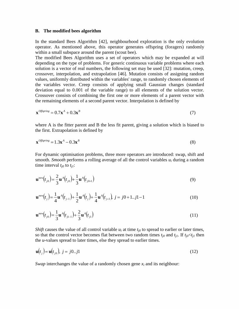
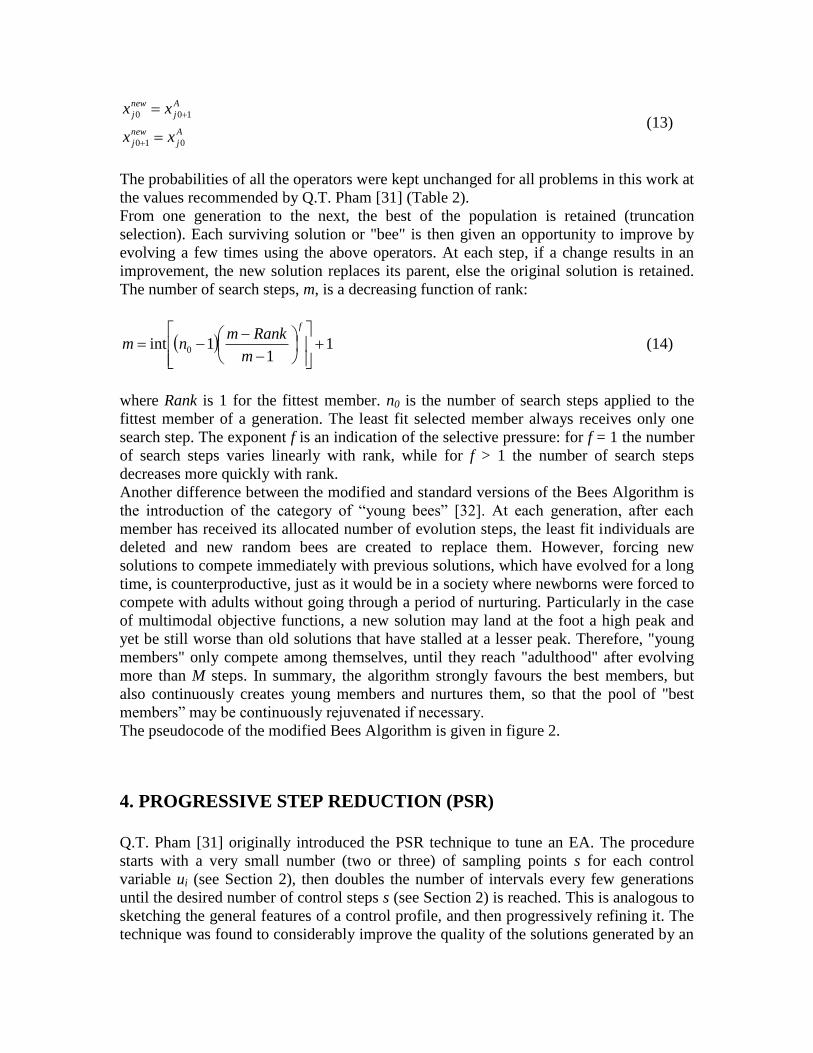
A
j
new
j
A
j
new
j
xx
xx
010
100
(13)
The probabilities of all the operators were kept unchanged for all problems in this work at
the values recommended by QT Pham [31] (Table 2)
From one generation to the next the best of the population is retained (truncation
selection) Each surviving solution or bee is then given an opportunity to improve by
evolving a few times using the above operators At each step if a change results in an
improvement the new solution replaces its parent else the original solution is retained
The number of search steps m is a decreasing function of rank
11
1int 0
f
m
Rankmnm (14)
where Rank is 1 for the fittest member n0 is the number of search steps applied to the
fittest member of a generation The least fit selected member always receives only one
search step The exponent f is an indication of the selective pressure for f = 1 the number
of search steps varies linearly with rank while for f gt 1 the number of search steps
decreases more quickly with rank
Another difference between the modified and standard versions of the Bees Algorithm is
the introduction of the category of ldquoyoung beesrdquo [32] At each generation after each
member has received its allocated number of evolution steps the least fit individuals are
deleted and new random bees are created to replace them However forcing new
solutions to compete immediately with previous solutions which have evolved for a long
time is counterproductive just as it would be in a society where newborns were forced to
compete with adults without going through a period of nurturing Particularly in the case
of multimodal objective functions a new solution may land at the foot a high peak and
yet be still worse than old solutions that have stalled at a lesser peak Therefore young
members only compete among themselves until they reach adulthood after evolving
more than M steps In summary the algorithm strongly favours the best members but
also continuously creates young members and nurtures them so that the pool of best
membersrdquo may be continuously rejuvenated if necessary
The pseudocode of the modified Bees Algorithm is given in figure 2
4 PROGRESSIVE STEP REDUCTION (PSR)
QT Pham [31] originally introduced the PSR technique to tune an EA The procedure
starts with a very small number (two or three) of sampling points s for each control
variable ui (see Section 2) then doubles the number of intervals every few generations
until the desired number of control steps s (see Section 2) is reached This is analogous to
sketching the general features of a control profile and then progressively refining it The
technique was found to considerably improve the quality of the solutions generated by an
evolutionary algorithm for a set of dynamic optimisation problems [31] In this study the
use of the PSR method to enhance the dynamic optimisation performance of the modified
Bees Algorithm is evaluated in the factorial experiment
5 MODIFIED BEES ALGORITHM PARAMETER TUNING
Compared to the standard version the modified Bees Algorithm is characterised by a
more sophisticated search procedure featuring a set of additional operators The action of
these operators is adjusted by tuning a number of system parameters Unfortunately
understanding and estimating precisely the effect of these parameters on the performance
of the algorithm is difficult and the task is complicated by interactions amongst different
operators
As a consequence of the need of tuning a relatively large number of system parameters
the optimisation of the modified Bees Algorithm via standard trial and error tuning [42] is
likely to be time consuming and may yield sub-optimal results Therefore the statistical
approach proposed by QT Pham [31] is used in this work This section discusses the
algorithm optimisation problem and describes the proposed procedure
A Tuning procedures for population-based algorithms
One of the main factors that make it hard to evaluate the effect of the tuning of a single
parameter on the algorithm‟s behaviour is the significant interactions between the action
of the different operators In addition global population-based metaheuristics of the kind
analysed in this paper are based on non-deterministic (stochastic) search processes As a
result the outcome of a single run of a procedure is not repeatable and the evaluation of
the effect of a given parameter setting is affected by a noise problem
Given an optimisation algorithm the No Free Lunch theorem [47] entails that there is no
universal tuning that works best on all possible problems Nevertheless classes of similar
mathematical and scientific problems share certain characteristic patterns which
correspond to regularities in the fitness landscape of the candidate solutions On these
classes of fitness landscapes some tunings work better than others That is each
parameter configuration allows the algorithm to exploit best the features of a given
number of optimisation problems and conversely is unsuitable to other problem domains
As a result for certain classes of problems it may be possible to derive a common tuning
based on a number of tests
The importance of matching each optimisation problem with the right configuration for
the optimiser has brought some researchers to consider parameter selection as one of the
most important elements in the building of a successful application [48]
The tuning of an algorithm is itself an optimisation task It can be considered as a multi-
objective optimisation problem where speed and robustness are often contradictory
requirements Most practitioners carry out at least some manual tuning of the algorithm
[49] In many cases due to the difficulty of tuning complex non-deterministic algorithms
the engineer needs to engage in time consuming trial and error procedures
Grefenstette [50] used an automatic meta-optimisation method where an EA is used to
optimise the performance of another EA Unfortunately due to the computational
complexity of this kind of algorithms the procedure is very time consuming for any non-
trivial application Moreover because of the noisy nature of the results of stochastic
search methods there is the problem of evaluating precisely the fitness of the candidate
solutions (ie parameter settings) More efficient meta-optimisation algorithms for
parameter tuning have been developed such as REVAC (Relevance Estimation and Value
Calibration of EA Parameters) [51 52] and Sequential Parameter Optimisation (SPO)
[53 54] Grid searches over the parameter space are sometimes used as in Francois and
Lavergne [55] where two parameters were optimised by discretising one parameter into
10 levels and the other into 20 levels While this gives a complete picture of the EA‟s
behaviour for the test problems considered it would be difficult to use this approach if
there are many more than two parameters to be tuned
Adaptive tuning is a popular and effective approach It was used to adapt the mutation
step size in evolutionary strategies by Rechenberg [56] and first applied to genetic
algorithms by Davis [57] A recent implementation uses the statistical outlier detection
method to estimate operator potentials and adjust operator frequencies [58] Another type
of adaptive tuning takes the form of competitive evolution between separate but
interacting populations of tuning solutions [46]
Adaptive tuning is conceptually attractive to users of population-based metaheuristics
However it does not come for free since some computational resources have to be spent
on the adaptation process On a more fundamental level adaptive tuning is a hill climbing
procedure (with some randomness arising from noise) and there is no guarantee that it
will converge to the global optimum This problem is mitigated if the gradient based
search is started from a promising starting point (ie a solution of high performance)
Recently QT Pham [31] proposed a statistics based tuning method where a two-level
factorial experiment is carried out with operator probabilities taking either a low (usually
zero) or high value in each test The effect of each operator is then quantified and the
results are used to tune the algorithm
B Two-level factorial experiment design
To investigate the usefulness of some of the features and get a rough tuning for the
others a two level full factorial experiment was carried out taking into account all the
combinations of the following variables values
Population size N 10 or 50
Progressive step reduction PSR Not used or used
Fraction of population chosen to survive based on fitness e 05 or 08
Fraction of young bees chosen to survive g 0 or 05
Maximum no of neighbourhood search steps per generation m 2 or 10
Linearity parameter f 2 or 5
Age at which young becomes adult M 5 or 10
In statistics terminology the first (lower) value is termed Level 1 and the second
(higher) value is termed Level +1
C Tuning procedure
The tuning procedure first described by QT Pham et al [32] was used The procedure is
based on the following principles
Parameter settings that cause poor performance must be avoided
If both (low and high) parameter settings are equally likely to yield poor
performance the parameter setting that is more likely to give good performance is
chosen
These principles are based on the observation that whilst the best runs usually give
results that are very similar the worst runs form a very long tail Moreover the results of
the worst runs are much further below the median than the results of the best runs are
above the median Therefore the main concern in tuning an algorithm is to prevent the
occurrence of bad runs
The best and worst settings are based on the weighted means of the top 10 and bottom
10 of the runs respectively For each setting five independent runs were executed for
benchmarks 2-8 and ten for benchmark 1 Preliminary investigations have indicated that
if fewer runs are used statistical fluctuations may become significant while if more are
used the differences between good and bad tunings are weakened The detailed tuning
procedure is given in Figure 3
Tables 3 and 4 give the best and worst levels of the parameters for the test problems and
their averages The clearest effect is that of population size N For all problems a low
population size gives better results The best level of N for each problem varies from
098 to 096 (Table 3) where 1 corresponds to a population size of 10 and +1 to one
of 50 On the other hand the worst level of N varies from +096 to +098
PSR does not always give the best results (half of the problems have a negative best
level for PSR which means that most of the best runs for those are without PSR in those
problems However the worst level of PSR varies from 075 to 097 (Table 4) Thus
although PSR may not always give the very best results it certainly provides a guarantee
against poor results and is worth applying Other parameters about which one can draw
definite conclusions are gr (avoid low level) and n0 (avoid low level) The effects of the
other parameters are ambiguous or neutral
Table 5 shows how the recommended tuning is calculated using the proposed procedure
The first row (after the headings) gives the weighted mean worst levels (bottom 10 of
runs) as calculated in the first step The second row converts the values to qualitative
judgments The third row gives the mean best levels in the second step of the procedure
The fourth row calculates the recommended levels according to step 4 of the procedure
The actual parameter settings are calculated from the recommended level (row 4) and the
definitions of high (row 5) and low (row 6) levels and entered in the last row
The recommended tuning according to the proposed factorial technique is given in the
last row of Table 5 With the only exception of PSR (which is applicable only to dynamic
control problems) the derived tuning is almost exactly the same as for the analytical test
problems considered by QT Pham et al [32] This might imply that within the
limitations imposed by the No Free Lunch theorem this parameter configuration is fairly
robust and relatively independent of the problems considered
6 EXPERIMENTAL SET UP
In order to evaluate the effectiveness of the modified Bees Algorithm its performance
was compared with that of the standard Bees Algorithm an EA and PSO All the four
optimisation algorithms encode the candidate solutions as ns-dimensional vectors of
decision variables as defined in equation [24] The duration of each algorithm is set to
obtain approximately the same number of function evaluations about 2000 (a lesser
number of evaluations gave insufficient separation between the algorithms for most of the
problems)
A Evolutionary Algorithm
The EA used in this work is described more in detail in [42] The parameters and
operators were chosen based on the results of a set of preliminary EA optimisation trials
The algorithm uses the fitness ranking procedure [43] to select the pool of reproducing
individuals Generational replacement with elitism [43] is employed to update the
population at the end of each evolution cycle
The mutation operator modifies the value of each of the variables of a solution of a small
amount This amount is randomly re-sampled for each variable with uniform probability
as follows
2
minmax xxrandomaxx oldnew
(15)
where x[xminxmax] is the variable being mutated random is a number drawn with
uniform probability in the interval [-11] and a is a system parameter defining the
maximum width of the mutation The parameter a is akin to ngh which determines the
neighbourhood of a standard Bees Algorithm‟s flower patch The mutation width a is
encoded in as an extra-variable in the chromosome of the individuals and is subjected to
the evolution process
Following the results of DT Pham and Castellani [42] genetic crossover is not
employed in the evolutionary procedure The preliminary optimisation trials confirmed
the superior performance of this configuration
Overall due to the lack of genetic recombinations the adaptation of the mutation width
and the real encoding of the solutions the EA procedure can be considered akin to the
Evolutionary programming [43] approach
The values of the EA learning parameters are shown in Table 6 They are set to obtain
2040 fitness evaluations per optimisation trial
B Particle Swarm Optimisation
The algorithm used in this study is the standard PSO procedure described by Kennedy
and Eberhart [44]
The movement (velocity) of each particle is defined by three elements namely the
particle‟s momentum personal experience (ie attraction force towards the best solution
found so far) and social interaction with its neighbours (ie attraction force towards the
best solution found by the neighbours) Each velocity vector component is clamped to the
range [minusvmax
i vmax
i] where
2
minmaxmax iii kv
(16)
The PSO parameters were set as recommended by Shi and Eberhart [59] except for the
connectivity (ie the number of neighbours per particle) and maximum speed which were
set according to experimental trial and error The maximum speed was adjusted via the
multiplication factor k (see eq 16) The values of the PSO learning parameters are
detailed in Table 7 They are set to obtain 2040 fitness evaluations per optimisation trial
C Standard Bees Algorithm
The procedure outlined in Section 3A was used The learning parameters were optimised
experimentally They are given in Table 10 They are set to obtain 2037 fitness
evaluations per optimisation trial
D Modified Bees Algorithm
The learning parameters and operator probabilities were set according to Tables 2 and 5
The algorithm is run for 57 evolution cycles which correspond to a total of 2031 fitness
evaluations per optimisation trial
7 EXPERIMENTAL RESULTS
The performance of each algorithm was evaluated on the average results of 30
independent optimisation trials The statistical significance of the differences of the
results obtained by the four algorithms was pairwise evaluated using Mann-Whitney U-
tests The U-tests were run for a 005 (5) level of significance
For each dynamic optimisation benchmark Table 9 reports the main statistical estimates
of the fitness of the solutions obtained by the four metaheuristics For each benchmark
the last column of Table 9 indicates the algorithm(s) that obtained the best results (ie
statistically significantly superior) Figures 4-11 visualise the median and 10th
and 90th
percentiles of the results obtained by the four algorithms Figure 12 shows the learning
curves of the modified Bees Algorithm for the eight benchmark problems The plots
show the evolution of the average minimum and maximum fitness of twenty
independent runs
The proposed optimisation method performed very effectively and consistently on most
of the dynamic optimisation problems In six cases out of eight the modified Bees
Algorithm ranked as the top performer The standard Bees Algorithm excelled on
benchmarks 4 and 8 whilst PSO obtained top results on function 3 Compared to PSO
the standard Bees Algorithm obtained better results in four cases comparable results (ie
no statistically significant difference) on three benchmarks and worst results in one case
In terms of robustness the two bees-inspired methods excelled This result is apparent
from the comparison of the standard deviation and upper and lower percentiles of the
distribution of the optimisation results With the exception of the trials on functions 3 and
8 the modified Bees Algorithm showed the most consistent performances The EA
consistently ranked as the worst in terms of quality of the solutions and robustness
In order to have a more complete evaluation of the competitiveness of the proposed
method the results obtained by the modified Bees Algorithm were compared with the
state-of-the-art in the literature
Table 10 shows for each benchmark the known optimum published in the literature the
optimum obtained by Rajesh et al [27] using Ant Colony Optimisation the optimum
achieved by QT Pham [31] using an evolutionary algorithm specially adapted for
dynamic optimisation (EADO) and the arithmetic mean of the fitness of the solutions
obtained in the 30 optimisation trials using the modified Bees Algorithm The result of
the best performing procedure is highlighted in bold The last column reports the
difference between the result achieved by the modified Bees Algorithm and the known
optimum expressed as a percentage of the optimum value
The figures referring to the known optima refer either to analytical results or the best-so-
far results obtained using other optimisation techniques The results taken from Rajesh et
al [27] are the average of 25 independent optimisation trials Unfortunately Rajesh and
his colleagues didn‟t specify which kind of average measure they used whether it was
the mean the median or other The results taken from QT Pham [31] are the arithmetic
mean of 10 independent runs
Notwithstanding the caveats due to the differences in the estimation of the average
solutions Table 10 allows to gauge the competitiveness of the proposed procedure In
five cases out of eight the modified Bees Algorithm gave the best optimisation results
The solutions generated by the modified Bees Algorithm were also very close in fitness
to the known optimum Namely they differed from the published optima by less than a
percentage point in six cases out of six and never more than 3
The experimental results highlighted also the effectiveness of the proposed parameter
tuning method Despite it was created only for a first rough adjustment of the system
parameters the procedure allowed to find a highly effective and consistent algorithm
configuration Compared to the customary tedious manual tuning process the proposed
tuning method proved to be a valid and effective alternative
8 CONCLUSIONS
This paper presented an application of a modified version of the Bees Algorithm to the
optimisation of dynamic control problems in chemical engineering Compared to the
standard Bees Algorithm the modified procedure uses an additional set of search
operators and allows newly generated bees to develop for a few optimisation cycles
without competing with mature individuals As a result of the enlarged set of operators a
relatively large set of system parameters needs to be adjusted in order to optimise the
performance of the modified Bees Algorithm These parameters are tuned using a
statistical tuning procedure
The performance of the proposed procedure was evaluated on a set of eight popular
dynamic optimisation problems The results obtained by the modified Bees Algorithm
were compared with those obtained using the standard procedure and other two well-
known nature-inspired optimisation methods The experimental results proved the
effectiveness and consistency of the proposed algorithm The performance of the
modified Bees Algorithm compared also well with that of the state-of-the-art methods in
the literature The solutions obtained using the modified Bees Algorithm were always
close to the known optima of the eight benchmarks
The results of the proposed work should not lead the reader to assume the superiority of
the modified Bees Algorithm over the other algorithms compared Indeed any such
interpretation is openly in contradiction with the No Free Lunch Theorem However this
study has demonstrated that the modified Bees Algorithm is capable to perform very
competitively on the kind of dynamic optimisation problems used
Experimental evidence has also proven the effectiveness of the statistical parameter
tuning method Despite being designed only for a first rough tuning of the parameters the
procedure obtained a high performing and robust algorithm configuration The usefulness
of the proposed tuning approach should also be evaluated in consideration of the
complexity and subjectivity of the standard trial-and-error procedures To be applied the
statistical parameter tuning technique requires only some knowledge of a reasonable
setting range (low and high levels) for each parameter
At the present the proposed tuning procedure was successfully applied to the
optimisation of EAs [31] and the modified Bees Algorithm ([32] and present work)
Further work should assess its effectiveness on other complex optimisation algorithms
The efficacy of the proposed statistical parameter tuning procedure should also be
compared to that of other procedures such as the Taguchi method [60]
ACKNOWLEDGMENT
The research described in this article was partially supported by the EC FP6 Innovative
Production Machines and Systems (IPROMS) Network of Excellence
List of References
[1] Pontryagin LS Boltyanski VG Gamkrelidze RV Mishchenko EF The
Mathematical Theory of Optimal Processes Wiley New York 1962
[2] Bryson A E Dynamic optimization Menlo Park CA Editorial Addison Wesley
Longman Inc 1999
[3] Srinivasan B Palanki S Bonvin D Dynamic optimization of batch processes I
Characterization of the nominal solution Computers and Chemical Engineering 27
2003 1-26
[4] Bellman R E Dynamic Programming Princeton NJ Princeton Univ Press 1957
[5] Dadebo SA McAuley KB Dynamic optimization of constrained chemical
engineering problems using dynamic programming Computers and Chemical
Engineering 19(5) 1995 513ndash525
[6] Luus R Optimal Control by Dynamic Programming Using Systematic Reduction in
Grid Size International Journal Control 51 1990 995ndash1013
[7] Luus R Application of dynamic programming to final state constrained optimal
control problems Hungarian Journal Industrial Chemistry 19 1991 245-254
[8] Lapidus L Luus R Optimal Control of Engineering Processes Waltham MA
Blaisdell Publishing 1967
[9] Bojkov B Luus R Evaluation of parameters used in iterative dynamic
programming Canadian Journal Chemical Engineering 71(3) 1993 451-459
[10] Luus R In search for global optima in nonlinear optimal control problems Proc
6th IASTED International Conference Aug 23-25 Honolulu 2004 394-399
[11] Biegler LT An overview of simultaneous strategies for dynamic optimization
Chemical Engineering and Processing Process Intensification 46(11) 2007 1043-
1053
[12] Goh C J Teo LK Control parameterization a unified app roach to optimal
control problems with general constraints Autornatica 24 1988 3-18
[13] Rangaiah GP Studies in Constrained Optimization of chemical process problems
Comput Chem Eng 9 1985 395-404
[14] Hargraves C R Paris S W Direct Trajectory Optimization Using Nonlinear
Programming and Collocation Journal of Guidance Control and Dynamics 10(4)
1987 338-342
[15] Edgar TF Himmelblau DM Optimization of Chemical Processes McGraw-Hill
New York 1989 369-371
[16] Binder T Cruse A Villar CAC Marquardt W Dynamic optimization using a
wavelet based adaptive control vector parameterization strategy Computers and
Chemical Engineering 24(2-7) 2000 1201ndash1207
[17] Garcia MSG Balsa-Canto E Alonso AA Banga JR Computing optimal
operating policies for the food industry Journal Food Engineering 74 2006 13ndash23
[18] Cizniar M Salhi D Fikar M Latifi MA Dynopt - Dynamic Optimisation Code
For Matlab httpwwwkirpchtfstubask~fikarresearchdynoptdynopthtm
[19] Goulcher R Casares Long JJ The solution of steady-state chemical engineering
optimisation problems using a random search algorithm Computers and Chemical
Engineering 2 1978 33-36
[20] Banga JR Irizarry-Rivera R Seider WD Stochastic optimization for optimal
and model-predictive control Computers and Chemical Engineering 22 1998 603-
612
[21] Li P Lowe K Arellano-Garcia H Wozny G Integration of simulated annealing
to a simulation tool for dynamic optimization of chemical processes Chemical
Engineering and Processing 39 2000 357ndash363
[22] Beyer HG and HP Schwefel Evolution strategies - A comprehensive
introduction Natural Computing 1(1) 2002 3ndash52
[23] Pham QT Dynamic optimization of chemical engineering processes by an
evolutionary method Computers and Chemical Engineering 22(7-8) 1998 1089-
1097
[24] Roubos JA van Straten G van Boxtel AJB An evolutionary strategy for fed-
batch bioreactor optimization Concepts and performance Journal of Biotechnology
67(2-3) 1999 173ndash187
[25] Michalewicz Z Janikow C Z Krawczyk J B A modified genetic algorithm for
optimal control problems Computers and Mathematics with Applications 23 1992
83-94
[26] Dorigo M Maniezzo V A Colorni Ant system optimization by a colony of
cooperating agents IEEE Transactions Systems Man and Cybernetics - Part B
26(1) 1996 29-41
[27] Rajesh J K Gupta HS Kusumakar VK Jayaraman and BD Kulkarni Dynamic
optimization of chemical processes using ant colony framework Computers and
Chemical Engineering 25(6) 2001 583ndash595
[28] Zhang B Chen D Zhao W Iterative ant-colony algorithm and its application to
dynamic optimization of chemical process Computers and Chemical Engineering
29(10) 2005 2078-2086
[29] Neri F Toivanen J Maumlkinen RAE An adaptive evolutionary algorithm with
intelligent mutation local searchers for designing multidrug therapies for HIV
Applied Intelligence 27 2007 219ndash235
[30] Pham D T Pham QT Castellani M Ghanbarzadeh A Dynamic optimisation
of chemical engineering process using the Bees Algorithm Proceedings 17th IFAC
(International Federation of Automatic Control) World Congress Seoul July 6-11
2008 httpwwwifac2008org paper 4047
[31] Pham QT Using Statistical Analysis to Tune an Evolutionary Algorithm for
Dynamic Optimization with Progressive Step Reduction Computers and Chemical
Engineering 31(11) 2007 1475-1483
[32] Pham QT Pham DT Castellani M A Modified Bees Algorithm and a
Statistics-Based Method for Tuning Its Parameters Proceedings of the Institution of
Mechanical Engineers Part I 225 2011 in press
[33] Ray WH Advanced process control New York McGraw-Hill 1981
[34] Renfro JG Morshedi AM Osbjornsen OA Simultaneous optimisation and
solution of systems described by differential algebraic equations Computers and
Chemical Engineering 11 1987 503-517
[35] Yeo BP A modified quasilinearization algorithm for the computation of optimal
singular control International Journal Control 32 1980 723-730
[36] Logsdon JS Biegler LT Accurate solution of differential-algebraic optimization
problems Industrial Engineering Chemistry Research 28(11) 1989 1628ndash1639
[37] Jackson R Optimization of chemical reactors with respect to flow configuration
Journal Optimisation Theory Applications 2(4) 1968 240-259
[38] Tieu D Cluett WR Penlidis A A comparison of collocation methods for solving
dynamic optimization problems Computers and Chemical Engineering 19(4) 1995
375-381
[39] Sarker RA Mohammadian M Yao X Evolutionary optimization Dordrecht
NL Kluwer Academic Publishers 2002
[40] Bonabeau E Dorigo M Theraulaz G Swarm intelligence from natural to
artificial systems New York Oxford University Press 1999
[41] Pham DT Ghanbarzadeh A Koc E Otri S The Bees Algorithm A Novel Tool
for Complex Optimisation Problems Proc 2nd Int Virtual Conf on Intelligent
Production Machines and Systems (IPROMS 2006) Oxford Elsevier 2006 454-
459
[42] Pham DT Castellani M The Bees Algorithm ndash Modelling Foraging Behaviour to
Solve Continuous Optimisation Problems Proceedings of the Institution of
Mechanical Engineers Part C 223(12) 2009 2919-2938
[43] Fogel DB Evolutionary Computation Toward a New Philosophy of Machine
Intelligence 2nd edition New York IEEE Press 2000
[44] Kennedy J Eberhart R Particle swarm optimization Edited by IEEE Neural
Networks Council Proceedings 1995 IEEE International Conference on Neural
Networks Perth AU IEEE Press Piscataway NJ 1995 1942-1948
[45] Seeley TD The Wisdom of the Hive The Social Physiology of Honey Bee
Colonies Cambridge Mass Harvard University Press 1996
[46] Pham QT Competitive evolution a natural approach to operator selection 956 in
Progress in Evolutionary Computation Lecture Notes in Artificial Intelligence by X
Yao Berlin Heidelberg Springer 1995 49-60
[47] Wolpert DH Macready WG No free lunch theorem for optimization IEEE
Transactions Evolutionary Computation 1(1) 1997 67-82
[48] Michalewicz M AE Eben and R Hinterding Parameter Selection In
Evolutionary Optimization by R Sarker M Mohammadian and X Yao Dordrecht
NL Kluwer Academic Press 2002 279-306
[49] De Jong KA An Analysis of the Behavior of a Class of Genetic Adaptive Systems
Ph D thesis University of Michigan 1975
[50] Grefenstette J Optimization of control parameters for genetic algorithms IEEE
Transactions on Systems Man and Cybernetics 16 1986 122-128
[51] Nannen V and AE Eiben Relevance Estimation and Value Calibration of
Evolutionary Algorithm Parameters Proceedings 20th International Joint Conference
Artificial Intelligence (IJCAI) Hyderabad India AAAI Press 2007 1034-1039
[52] Smit S and A Eiben Parameter Tuning of Evolutionary Algorithms Generalist vs
Specialist In Applications of Evolutionary Computation edited by C Di Chio et al
Berlin Heidelberg Springer 2010 542-551
[53] Bartz-Beielstein T CWG Lasarczyk and M Preuss Sequential Parameter
Optimization Proceedings 2005 IEEE Congress on Evolutionary Computation
(CEC05) Edinburgh Scotland 2005 773-780
[54] Preuss M and T Bartz-Beielstein Sequential Parameter Optimization Applied to
Self-Adaptation for Binary-Coded Evolutionary Algorithms In Parameter Setting in
Evolutionary Algorithms edited by FG Lobo CF Lima and Z Michalewicz
Heidelberg Springer-Verlag 2007 91-119
[55] Francois O and C Lavergne Design of evolutionary algorithms - a statistical
perspective IEEE Transactions Evolutionary Computations 5 2001 129ndash48
[56] Rechenberg I Evolutionsstrategie Optimierung technischer Systeme und Prinzipien
der biologischen Evolution Stuttgart D Frommann-Holzboog 1973
[57] Davis L Adapting operator probabilities in genetic algorithms Proceedings of the
Third International Conference on Genetic Algorithms and Their Applications San
Mateo CA Morgan Kaufman 1989
[58] Whitacre JM QT Pham and RA Sarker Use of Statistical Outlier Detection
Method in Adaptive Evolutionary Algorithms Proceedings of the 8th annual
conference on Genetic and evolutionary computation (GECCO) Seattle WA ACM
Press New York NY 2006 1345-1352
[59] Shi Y and R Eberhart Parameter Selection in Particle Swarm Optimization
Proceedings of the 1998 Annual Conference on Evolutionary Programming San
Diego CA Lecture Notes in Computer Science 1447 Springer 1998 591-600
[60] Roy RK Design of Experiments Using The Taguchi Approach 16 Steps to Product
and Process Improvement New York John Wiley and Sons Ltd 2001
List of Tables
Table 1 Test objective functions
Table 2 Operator probabilities
Table 3 Best levels of parameters
Table 4 Worst levels of parameters
Table 5 Tuning of algorithm for dynamic control optimisation problems
Table 6 EA learning parameters
Table 7 PSO learning parameters
Table 8 Standard Bees Algorithm learning parameters
Table 9 Experimental results
Table 10 Comparison with literature
List of Figures
Figure 1 Pseudocode of standard Bees Algorithm
Figure 2 Pseudocode of modified Bees Algorithm
Figure 3 Detailed Bees Algorithm tuning procedure
Figure 4 Function 1 - optimisation results (median 10-90 percentile) for algorithms tested
Figure 5 Function 2 - optimisation results (median 10-90 percentile) for algorithms tested
Figure 6 Function 3 - optimisation results (median 10-90 percentile) for algorithms tested
Figure 7 Function 4 - optimisation results (median 10-90 percentile) for algorithms tested
Figure 8 Function 5 - optimisation results (median 10-90 percentile) for algorithms tested
Figure 9 Function 6 - optimisation results (median 10-90 percentile) for algorithms tested
Figure 10 Function 7 - optimisation results (median 10-90 percentile) for algorithms tested
Figure 11 Function 8 - optimisation results (median 10-90 percentile) for algorithms tested
Figure 12 Learning curves of the modified Bees Algorithm
Appendix A
Dynamic optimisation benchmarks
Function 1 CSTR
Steps=19
Initialisation y=[01883 02507 00476 00899 01804 01394 01046 00]
Constraints 0leu1le20 0leu1le6 0leu1le4 0leu1le20
0lttlt4
Maximise y8
Function 2 Batch reactor consecutive reactions
Steps=39
Initialisation y=[10 00]
Constraints 298leule398
0lttlt1
Maximise y2
Function 3 Nonlinear unconstrained mathematical system
Steps=31
Initialisation
Constraints -4leule10
0lttlt1
Minimise y4
Function 4 Unconstrained mathematical system
Steps=15
Initialisation y=[10 00]
Constraints -2leule2
0lttlt1
Minimise y2
Function 5 Tubular reactor parallel reaction
Steps=19
Initialisation y=[10 00]
Constraints 0leule5
0lttlt1
Maximise y2
Function 6 Plug flow reactor catalyst blend
Steps=39
Initialisation y=[10 00]
Constraints 0leule1
0lttlt12
Maximise 1-y1-y2
Function 7 Consecutive reaction
Steps=19
Initialisation y=[10 00]
Constraints 300leule1000
0lttlt125
Maximise y1
Function 8 Constrained mathematical system
Same as Function 4
Constraint y1=10
Figure 1 Pseudocode of standard Bees Algorithm
Initialise N random solutions
Iterate until a stopping criterion is met
Evaluate the fitness of the population
Sort the solutions according to their fitness
waggle dance Select the highest-ranking m solutions for neighbourhood search
Assign x=ne foragers to each of the em top-ranking elite solutions
Assign x=nbne foragers to each of the remaining m-e selected solutions
local search For each of the m selected solutions
Create x new solutions by perturbing the selected solution randomly or otherwise
Evaluate the new solutions
Retain the best solution amongst the selected and new solutions Adjust the neighbourhood of the retained solution
Re-initialise sites where search has stagnated for a given number of iterations
global search Repeat N-m times
Generate randomly a new solution
Evaluate the new solution
Form new population (m solutions from local search N-m from global search)
Figure 1
Figure 2 Pseudocode of modified Bees Algorithm
Initiate N random bees
Iterate
Sort all the bees in the present population
Select the e fittest bees into the new population
Sort the young bees (age M) in the present population
Select the g fittest young bees into the new population
Create Neg random new bees and put them in the new population
Let each bee evolve m times where m is given by eq (14) ()
Until a stopping criterion is met
() In the evolution steps an offspring replaces its parent only if it is better than the
parent
Figure 2
Figure 3 Detailed Bees Algorithm tuning procedure
1 Calculate the weighted mean level of the parameters in the worst 10 of
the runs (-1 is the low level of the factor +1 is the high level) Weights are
adjusted to vary linearly with rank the worst run having a weight of 1 the
10-th percentile a weight of 0 This gives the mean worst settings for the
problem
2 Calculate the weighted mean level of the parameters in the best 10 of the
runs in same manner (best run has maximum weight) This gives the mean
best settings for the problem
3 Repeat steps 1 amp 2 for several test problems and calculate the overall mean
ldquobestrdquo and ldquoworstrdquo level of each parameter
4 If the mean worst level of a parameter is low (from -1 to 033) set that
parameter to the maximum level If the mean worst level of a parameter is
high (from +033 to +1) set that parameter to the minimum level In other
cases (from 033 to +033) set that parameter to the average of the best
tunings
Figure 3
Box Plot of Function 1 grouped by Algorithm
maximisation task
Median
10-90
modBA stdBA PSO EA
Algorithm
305
310
315
320
325
330
335
340
345
Fu
nctio
n 1
Figure 4 Function 1 - optimisation results (median 10-90 percentile) for algorithms tested
Figure 4
Box Plot of Function 2 grouped by Algorithm
maximisation task
Median
10-90
modBA stdBA PSO EA
Algorithm
06060
06065
06070
06075
06080
06085
06090
06095
06100
06105
06110
Fu
nctio
n 2
Figure 5 Function 2 - optimisation results (median 10-90 percentile) for algorithms tested
Figure 5
Box Plot of Function 3 grouped by Algorithm
minimisation task
Median
10-90
modBA stdBA PSO EA
Algorithm
0115
0120
0125
0130
0135
0140
0145
0150
0155
Fu
nctio
n 3
Figure 6 Function 3 - optimisation results (median 10-90 percentile) for algorithms tested
Figure 6
Box Plot of Function 4 grouped by Algorithm
minimisation task
Median
10-90
modBA stdBA PSO EA
Algorithm
075
076
077
078
079
080
081
082
Fu
nctio
n4
Figure 7 Function 4 - optimisation results (median 10-90 percentile) for algorithms tested
Figure 7
Box Plot of Function 5 grouped by Algorithm
maximisation task
Median
10-90
modBA stdBA PSO EA
Algorithm
0556
0558
0560
0562
0564
0566
0568
0570
0572
0574
0576
Fu
nctio
n 5
Figure 8 Function 5 - optimisation results (median 10-90 percentile) for algorithms tested
Figure 8
Box Plot of Function 6 grouped by Algorithm
maximisation task
Median
10-90
modBA stdBA PSO EA
Algorithm
0466
0468
0470
0472
0474
0476
0478
Fu
nctio
n 6
Figure 9 Function 6 - optimisation results (median 10-90 percentile) for algorithms tested
Figure 9
Box Plot of Function 7 grouped by Algorithm
maximisation task
Median
10-90
modBA stdBA PSO EA
Algorithm
0466
0468
0470
0472
0474
0476
0478
0480
0482
Fu
nctio
n 7
Figure 10 Function 7 - optimisation results (median 10-90 percentile) for algorithms tested
Figure 10
Box Plot of Function 8 grouped by Algorithm
minimisation task
Median
10-90
modBA stdBA PSO EA
Algorithm
091
092
093
094
095
096
097
098
099
100
Fu
nctio
n 8
Figure 11 Function 8 - optimisation results (median 10-90 percentile) for algorithms tested
Figure 11
Figure 12 Learning curves of the modified Bees Algorithm
Figure 12
Table 1 Test objective functions
no References Optimum from
literature m n s
Type of
problem Description
1
Pham QT [4 9] Lapidus
and Luus [11] Bojkov and
Luus [12]
3391 8 4 19 maximisation CSTR
2
Dadebo and McAuley [2]
Rajesh et al [7] Ray [13]
Renfro Morshedi and
Osbjornsen [14]
061077 2 1 39 maximisation
Batch reactor consecutive reactions
ABC
3 Rajesh et al [7] Yeo [15]
Luus [16] 012011 4 1 31 minimisation
Nonlinear
unconstrained
mathematical system
4 Rajesh et al [7] Luus [17] 076159 2 1 15 minimisation Unconstrained math
system
5
Dadebo and McAuley [2]
Rajesh et al [7] Logsdon and Biegler [18]
057353 2 1 19 maximisation Tubular reactor
parallel reaction
6
Dadebo and McAuley [2]
Rajesh et al [7] Jackson
[19]
047695 2 1 39 maximisation
Plug flow reactor
catalyst blend
ABC
7 Rajesh et al [7] Tieu
Cluett and Penlidis [20] 048005 2 1 19 maximisation
Consecutive
reactions ABC
8 Rajesh et al [7] Luus [17]
Constraint y1(tf)=1 092518 2 1 15 minimisation
Constrained
mathematical system
Table 1
Table 2 Operator probabilities
Extrapolate 02
Crossover 0
Interpolate 0
Mutation 005
Creep 05
Swap 0
Shift 02
Smooth 005
Table 2
Table 3 Best levels of parameters
Problem N PSR er gr n0 f M
1 -097 -071 -018 035 063 015 021
2 -098 096 -012 025 098 022 -003
3 -097 017 -006 056 004 029 010
4 -097 -050 -027 039 027 018 -002
5 -096 090 028 030 074 -035 008
6 -097 028 -022 048 049 038 -009
7 -097 -091 -010 015 087 036 -004
8 -095 -033 -018 047 044 023 031
Mean best level -097 -002 -010 037 056 019 006
Table 3
Table 4 Worst levels of parameters
Problem N PSR er gr n0 f M
1 097 -077 -003 -081 -072 -009 -015
2 098 -098 -007 -063 -078 -011 -004
3 097 -097 010 -064 -071 -007 -010
4 097 -075 -004 -032 -057 -007 017
5 097 -097 -001 -074 -079 -008 -004
6 097 -097 005 -054 -085 -003 004
7 097 -097 007 -048 -079 -017 001
8 096 -097 001 -050 -066 -018 -010
Mean worst level 097 -092 001 -058 -074 -010 -003
Table 4
Table 5 Tuning of algorithm for dynamic control optimisation problems
Parameter N PSR er gr n0 f M
Worst level (1 to +1) 097 -092 001 -058 -074 -010 -003
Worst (HighLowIndifferent) H L I L L I I
Best level (-1 to +1) -097 -002 -010 037 056 019 006
Recommended level (-1 to +1) -1 1 -010 1 1 -010 -003
Level 1 parameter value 100 No 05 00 2 20 50
Level +1 parameter value 500 Yes 08 05 10 50 100
Recommended actual value 10 Yes 07 07 10 25 7
Table 5
Table 6 EA learning parameters
Parameter Value
Population size 20
Children per generation 19
Mutation rate (variables) 08
Mutation rate (mutation width) 08
Initial mutation interval width a (variables) 01
Initial mutation interval width (mutation width) 01
Number of evaluations per iteration 20
Number of iterations 102
Total number of fitness evaluations 1040
Table 6
Table 7 PSO learning parameters
Parameter Value
Population size 20
Connectivity (no of neighbours) 4
Maximum velocity (k) 01
c1 20
c2 20
inertia weight at start wmax 09
inertia weight at end wmin 04
Number of evaluations per iteration 20
Number of iterations 102
Total number of fitness evaluations 1040
Table 7
Table 8 Standard Bees Algorithm learning parameters
Parameter Name Value
number of scout bees ns 1
number of elite sites ne 1
number of best sites nb 3
recruited bees for elite sites nre 10
recruited bees for remaining best sites nrb 5
initial size of neighbourhood ngh 05
limit of stagnation cycles for site abandonment stlim 10
Number of evaluations per iteration ev 21
Number of iterations 97
Total number of fitness evaluations 2037
Table 8
Table 9 Experimental results
Function 1 - maximisation task
Mean Std dev Median 10th Perc 90
th Perc Best
Mod BA 3386855 03502 3387670 3382505 3390647 X
Std BA 3284946 17868 3283990 3261050 3308190
PSO 3343692 05269 3344450 3336685 3349475
EA 3121288 37074 3126080 3065485 3169305
Function 2 - maximisation task
Mod BA 06107 00000 06107 06107 06108 X
Std BA 06103 00002 06104 06100 06105
PSO 06102 00003 06103 06099 06104
EA 06074 00010 06074 06064 06088
Function 3 - minimisation task
Mod BA 01238 00065 01206 01202 01363 X
Std BA 01325 00014 01323 01309 01346
PSO 01313 00022 01308 01296 01331 X
EA 01398 00066 01376 01337 01504
Function 4 - minimisation task
Mod BA 07618 00001 07617 07617 07619
Std BA 07595 00000 07595 07595 07595 X
PSO 07624 00018 07621 07604 07652
EA 07865 00238 07779 07682 08172
Function 5 - maximisation task
Mod BA 05733 00001 05734 05732 05735 X
Std BA 05718 00011 05722 05699 05729
PSO 05709 00016 05714 05696 05724
EA 05634 00057 05644 05575 05681
Function 6 - maximisation task
Mod BA 04772 00002 04773 04769 04774 X
Std BA 04758 00004 04759 04752 04762
PSO 04736 00011 04738 04725 04748
EA 04697 00016 04696 04675 04719
Function 7 - maximisation task
Mod BA 04800 00001 04800 04799 04801 X
Std BA 04795 00003 04796 04795 04796
PSO 04745 00036 04754 04687 04789
EA 04716 00048 04720 04683 04763
Function 8 - minimisation task
Mod BA 09378 00095 09355 09275 09534
Std BA 09211 00006 09209 09206 09219 X
PSO 09301 00114 09247 09226 09476
EA 09644 00326 09544 09288 09938
Table 9
Table 10 Comparison with literature
Function Task Literature Ant
Algorithm [7] EADO [9] Modified BA
1 maximisation 3391000 - 3389200 3386855 01224
2 maximisation 06108 06105 06107 06107 00115
3 minimisation 01201 01290 01241 01238 29806
4 minimisation 07616 07624 07616 07618 00276
5 maximisation 05735 05728 05733 05733 00401
6 maximisation 04770 04762 04770 04772 00524
7 maximisation 04801 04793 04800 04800 00104
8 minimisation 09252 09255 09584 09378 13457
Table 10
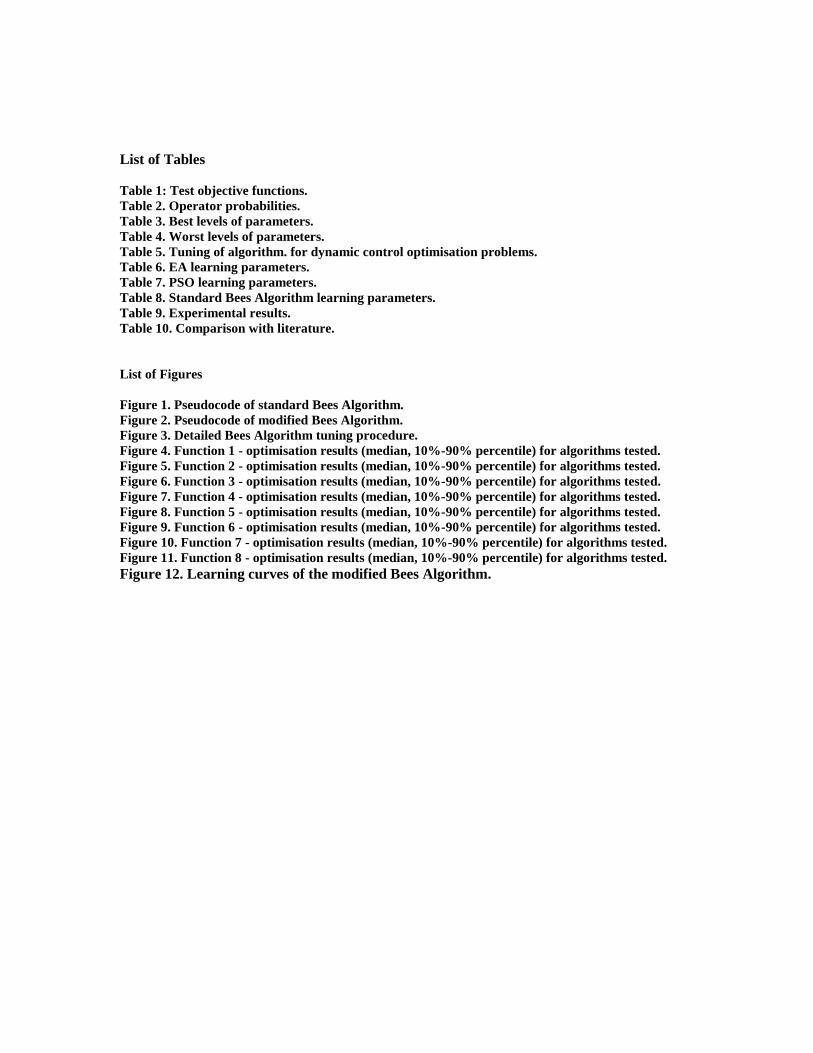
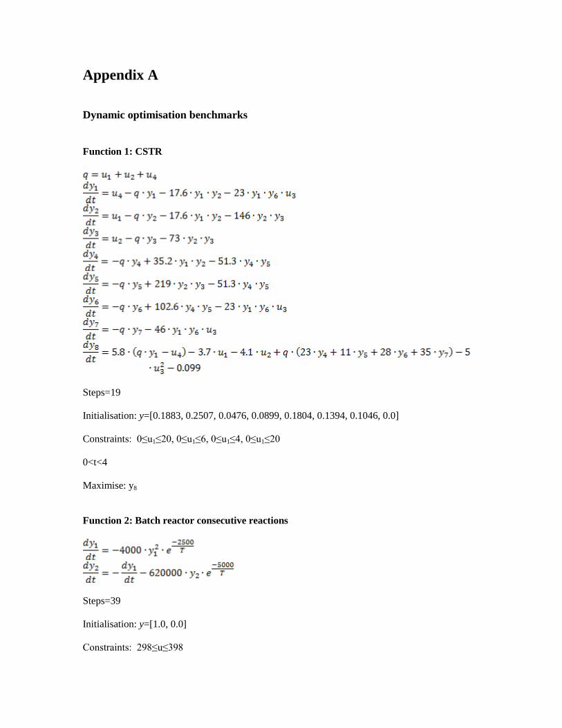
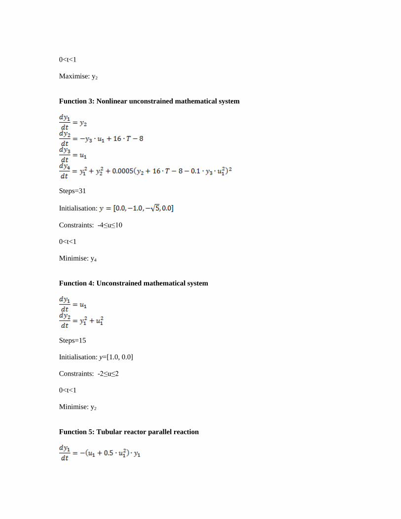
0lttlt1
Maximise y2
Function 3 Nonlinear unconstrained mathematical system
Steps=31
Initialisation
Constraints -4leule10
0lttlt1
Minimise y4
Function 4 Unconstrained mathematical system
Steps=15
Initialisation y=[10 00]
Constraints -2leule2
0lttlt1
Minimise y2
Function 5 Tubular reactor parallel reaction
Steps=19
Initialisation y=[10 00]
Constraints 0leule5
0lttlt1
Maximise y2
Function 6 Plug flow reactor catalyst blend
Steps=39
Initialisation y=[10 00]
Constraints 0leule1
0lttlt12
Maximise 1-y1-y2
Function 7 Consecutive reaction
Steps=19
Initialisation y=[10 00]
Constraints 300leule1000
0lttlt125
Maximise y1
Function 8 Constrained mathematical system
Same as Function 4
Constraint y1=10
Figure 1 Pseudocode of standard Bees Algorithm
Initialise N random solutions
Iterate until a stopping criterion is met
Evaluate the fitness of the population
Sort the solutions according to their fitness
waggle dance Select the highest-ranking m solutions for neighbourhood search
Assign x=ne foragers to each of the em top-ranking elite solutions
Assign x=nbne foragers to each of the remaining m-e selected solutions
local search For each of the m selected solutions
Create x new solutions by perturbing the selected solution randomly or otherwise
Evaluate the new solutions
Retain the best solution amongst the selected and new solutions Adjust the neighbourhood of the retained solution
Re-initialise sites where search has stagnated for a given number of iterations
global search Repeat N-m times
Generate randomly a new solution
Evaluate the new solution
Form new population (m solutions from local search N-m from global search)
Figure 1
Figure 2 Pseudocode of modified Bees Algorithm
Initiate N random bees
Iterate
Sort all the bees in the present population
Select the e fittest bees into the new population
Sort the young bees (age M) in the present population
Select the g fittest young bees into the new population
Create Neg random new bees and put them in the new population
Let each bee evolve m times where m is given by eq (14) ()
Until a stopping criterion is met
() In the evolution steps an offspring replaces its parent only if it is better than the
parent
Figure 2
Figure 3 Detailed Bees Algorithm tuning procedure
1 Calculate the weighted mean level of the parameters in the worst 10 of
the runs (-1 is the low level of the factor +1 is the high level) Weights are
adjusted to vary linearly with rank the worst run having a weight of 1 the
10-th percentile a weight of 0 This gives the mean worst settings for the
problem
2 Calculate the weighted mean level of the parameters in the best 10 of the
runs in same manner (best run has maximum weight) This gives the mean
best settings for the problem
3 Repeat steps 1 amp 2 for several test problems and calculate the overall mean
ldquobestrdquo and ldquoworstrdquo level of each parameter
4 If the mean worst level of a parameter is low (from -1 to 033) set that
parameter to the maximum level If the mean worst level of a parameter is
high (from +033 to +1) set that parameter to the minimum level In other
cases (from 033 to +033) set that parameter to the average of the best
tunings
Figure 3
Box Plot of Function 1 grouped by Algorithm
maximisation task
Median
10-90
modBA stdBA PSO EA
Algorithm
305
310
315
320
325
330
335
340
345
Fu
nctio
n 1
Figure 4 Function 1 - optimisation results (median 10-90 percentile) for algorithms tested
Figure 4
Box Plot of Function 2 grouped by Algorithm
maximisation task
Median
10-90
modBA stdBA PSO EA
Algorithm
06060
06065
06070
06075
06080
06085
06090
06095
06100
06105
06110
Fu
nctio
n 2
Figure 5 Function 2 - optimisation results (median 10-90 percentile) for algorithms tested
Figure 5
Box Plot of Function 3 grouped by Algorithm
minimisation task
Median
10-90
modBA stdBA PSO EA
Algorithm
0115
0120
0125
0130
0135
0140
0145
0150
0155
Fu
nctio
n 3
Figure 6 Function 3 - optimisation results (median 10-90 percentile) for algorithms tested
Figure 6
Box Plot of Function 4 grouped by Algorithm
minimisation task
Median
10-90
modBA stdBA PSO EA
Algorithm
075
076
077
078
079
080
081
082
Fu
nctio
n4
Figure 7 Function 4 - optimisation results (median 10-90 percentile) for algorithms tested
Figure 7
Box Plot of Function 5 grouped by Algorithm
maximisation task
Median
10-90
modBA stdBA PSO EA
Algorithm
0556
0558
0560
0562
0564
0566
0568
0570
0572
0574
0576
Fu
nctio
n 5
Figure 8 Function 5 - optimisation results (median 10-90 percentile) for algorithms tested
Figure 8
Box Plot of Function 6 grouped by Algorithm
maximisation task
Median
10-90
modBA stdBA PSO EA
Algorithm
0466
0468
0470
0472
0474
0476
0478
Fu
nctio
n 6
Figure 9 Function 6 - optimisation results (median 10-90 percentile) for algorithms tested
Figure 9
Box Plot of Function 7 grouped by Algorithm
maximisation task
Median
10-90
modBA stdBA PSO EA
Algorithm
0466
0468
0470
0472
0474
0476
0478
0480
0482
Fu
nctio
n 7
Figure 10 Function 7 - optimisation results (median 10-90 percentile) for algorithms tested
Figure 10
Box Plot of Function 8 grouped by Algorithm
minimisation task
Median
10-90
modBA stdBA PSO EA
Algorithm
091
092
093
094
095
096
097
098
099
100
Fu
nctio
n 8
Figure 11 Function 8 - optimisation results (median 10-90 percentile) for algorithms tested
Figure 11
Figure 12 Learning curves of the modified Bees Algorithm
Figure 12
Table 1 Test objective functions
no References Optimum from
literature m n s
Type of
problem Description
1
Pham QT [4 9] Lapidus
and Luus [11] Bojkov and
Luus [12]
3391 8 4 19 maximisation CSTR
2
Dadebo and McAuley [2]
Rajesh et al [7] Ray [13]
Renfro Morshedi and
Osbjornsen [14]
061077 2 1 39 maximisation
Batch reactor consecutive reactions
ABC
3 Rajesh et al [7] Yeo [15]
Luus [16] 012011 4 1 31 minimisation
Nonlinear
unconstrained
mathematical system
4 Rajesh et al [7] Luus [17] 076159 2 1 15 minimisation Unconstrained math
system
5
Dadebo and McAuley [2]
Rajesh et al [7] Logsdon and Biegler [18]
057353 2 1 19 maximisation Tubular reactor
parallel reaction
6
Dadebo and McAuley [2]
Rajesh et al [7] Jackson
[19]
047695 2 1 39 maximisation
Plug flow reactor
catalyst blend
ABC
7 Rajesh et al [7] Tieu
Cluett and Penlidis [20] 048005 2 1 19 maximisation
Consecutive
reactions ABC
8 Rajesh et al [7] Luus [17]
Constraint y1(tf)=1 092518 2 1 15 minimisation
Constrained
mathematical system
Table 1
Table 2 Operator probabilities
Extrapolate 02
Crossover 0
Interpolate 0
Mutation 005
Creep 05
Swap 0
Shift 02
Smooth 005
Table 2
Table 3 Best levels of parameters
Problem N PSR er gr n0 f M
1 -097 -071 -018 035 063 015 021
2 -098 096 -012 025 098 022 -003
3 -097 017 -006 056 004 029 010
4 -097 -050 -027 039 027 018 -002
5 -096 090 028 030 074 -035 008
6 -097 028 -022 048 049 038 -009
7 -097 -091 -010 015 087 036 -004
8 -095 -033 -018 047 044 023 031
Mean best level -097 -002 -010 037 056 019 006
Table 3
Table 4 Worst levels of parameters
Problem N PSR er gr n0 f M
1 097 -077 -003 -081 -072 -009 -015
2 098 -098 -007 -063 -078 -011 -004
3 097 -097 010 -064 -071 -007 -010
4 097 -075 -004 -032 -057 -007 017
5 097 -097 -001 -074 -079 -008 -004
6 097 -097 005 -054 -085 -003 004
7 097 -097 007 -048 -079 -017 001
8 096 -097 001 -050 -066 -018 -010
Mean worst level 097 -092 001 -058 -074 -010 -003
Table 4
Table 5 Tuning of algorithm for dynamic control optimisation problems
Parameter N PSR er gr n0 f M
Worst level (1 to +1) 097 -092 001 -058 -074 -010 -003
Worst (HighLowIndifferent) H L I L L I I
Best level (-1 to +1) -097 -002 -010 037 056 019 006
Recommended level (-1 to +1) -1 1 -010 1 1 -010 -003
Level 1 parameter value 100 No 05 00 2 20 50
Level +1 parameter value 500 Yes 08 05 10 50 100
Recommended actual value 10 Yes 07 07 10 25 7
Table 5
Table 6 EA learning parameters
Parameter Value
Population size 20
Children per generation 19
Mutation rate (variables) 08
Mutation rate (mutation width) 08
Initial mutation interval width a (variables) 01
Initial mutation interval width (mutation width) 01
Number of evaluations per iteration 20
Number of iterations 102
Total number of fitness evaluations 1040
Table 6
Table 7 PSO learning parameters
Parameter Value
Population size 20
Connectivity (no of neighbours) 4
Maximum velocity (k) 01
c1 20
c2 20
inertia weight at start wmax 09
inertia weight at end wmin 04
Number of evaluations per iteration 20
Number of iterations 102
Total number of fitness evaluations 1040
Table 7
Table 8 Standard Bees Algorithm learning parameters
Parameter Name Value
number of scout bees ns 1
number of elite sites ne 1
number of best sites nb 3
recruited bees for elite sites nre 10
recruited bees for remaining best sites nrb 5
initial size of neighbourhood ngh 05
limit of stagnation cycles for site abandonment stlim 10
Number of evaluations per iteration ev 21
Number of iterations 97
Total number of fitness evaluations 2037
Table 8
Table 9 Experimental results
Function 1 - maximisation task
Mean Std dev Median 10th Perc 90
th Perc Best
Mod BA 3386855 03502 3387670 3382505 3390647 X
Std BA 3284946 17868 3283990 3261050 3308190
PSO 3343692 05269 3344450 3336685 3349475
EA 3121288 37074 3126080 3065485 3169305
Function 2 - maximisation task
Mod BA 06107 00000 06107 06107 06108 X
Std BA 06103 00002 06104 06100 06105
PSO 06102 00003 06103 06099 06104
EA 06074 00010 06074 06064 06088
Function 3 - minimisation task
Mod BA 01238 00065 01206 01202 01363 X
Std BA 01325 00014 01323 01309 01346
PSO 01313 00022 01308 01296 01331 X
EA 01398 00066 01376 01337 01504
Function 4 - minimisation task
Mod BA 07618 00001 07617 07617 07619
Std BA 07595 00000 07595 07595 07595 X
PSO 07624 00018 07621 07604 07652
EA 07865 00238 07779 07682 08172
Function 5 - maximisation task
Mod BA 05733 00001 05734 05732 05735 X
Std BA 05718 00011 05722 05699 05729
PSO 05709 00016 05714 05696 05724
EA 05634 00057 05644 05575 05681
Function 6 - maximisation task
Mod BA 04772 00002 04773 04769 04774 X
Std BA 04758 00004 04759 04752 04762
PSO 04736 00011 04738 04725 04748
EA 04697 00016 04696 04675 04719
Function 7 - maximisation task
Mod BA 04800 00001 04800 04799 04801 X
Std BA 04795 00003 04796 04795 04796
PSO 04745 00036 04754 04687 04789
EA 04716 00048 04720 04683 04763
Function 8 - minimisation task
Mod BA 09378 00095 09355 09275 09534
Std BA 09211 00006 09209 09206 09219 X
PSO 09301 00114 09247 09226 09476
EA 09644 00326 09544 09288 09938
Table 9
Table 10 Comparison with literature
Function Task Literature Ant
Algorithm [7] EADO [9] Modified BA
1 maximisation 3391000 - 3389200 3386855 01224
2 maximisation 06108 06105 06107 06107 00115
3 minimisation 01201 01290 01241 01238 29806
4 minimisation 07616 07624 07616 07618 00276
5 maximisation 05735 05728 05733 05733 00401
6 maximisation 04770 04762 04770 04772 00524
7 maximisation 04801 04793 04800 04800 00104
8 minimisation 09252 09255 09584 09378 13457
Table 10
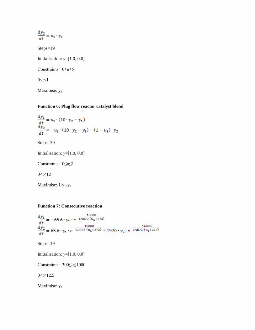
Steps=19
Initialisation y=[10 00]
Constraints 0leule5
0lttlt1
Maximise y2
Function 6 Plug flow reactor catalyst blend
Steps=39
Initialisation y=[10 00]
Constraints 0leule1
0lttlt12
Maximise 1-y1-y2
Function 7 Consecutive reaction
Steps=19
Initialisation y=[10 00]
Constraints 300leule1000
0lttlt125
Maximise y1
Function 8 Constrained mathematical system
Same as Function 4
Constraint y1=10
Figure 1 Pseudocode of standard Bees Algorithm
Initialise N random solutions
Iterate until a stopping criterion is met
Evaluate the fitness of the population
Sort the solutions according to their fitness
waggle dance Select the highest-ranking m solutions for neighbourhood search
Assign x=ne foragers to each of the em top-ranking elite solutions
Assign x=nbne foragers to each of the remaining m-e selected solutions
local search For each of the m selected solutions
Create x new solutions by perturbing the selected solution randomly or otherwise
Evaluate the new solutions
Retain the best solution amongst the selected and new solutions Adjust the neighbourhood of the retained solution
Re-initialise sites where search has stagnated for a given number of iterations
global search Repeat N-m times
Generate randomly a new solution
Evaluate the new solution
Form new population (m solutions from local search N-m from global search)
Figure 1
Figure 2 Pseudocode of modified Bees Algorithm
Initiate N random bees
Iterate
Sort all the bees in the present population
Select the e fittest bees into the new population
Sort the young bees (age M) in the present population
Select the g fittest young bees into the new population
Create Neg random new bees and put them in the new population
Let each bee evolve m times where m is given by eq (14) ()
Until a stopping criterion is met
() In the evolution steps an offspring replaces its parent only if it is better than the
parent
Figure 2
Figure 3 Detailed Bees Algorithm tuning procedure
1 Calculate the weighted mean level of the parameters in the worst 10 of
the runs (-1 is the low level of the factor +1 is the high level) Weights are
adjusted to vary linearly with rank the worst run having a weight of 1 the
10-th percentile a weight of 0 This gives the mean worst settings for the
problem
2 Calculate the weighted mean level of the parameters in the best 10 of the
runs in same manner (best run has maximum weight) This gives the mean
best settings for the problem
3 Repeat steps 1 amp 2 for several test problems and calculate the overall mean
ldquobestrdquo and ldquoworstrdquo level of each parameter
4 If the mean worst level of a parameter is low (from -1 to 033) set that
parameter to the maximum level If the mean worst level of a parameter is
high (from +033 to +1) set that parameter to the minimum level In other
cases (from 033 to +033) set that parameter to the average of the best
tunings
Figure 3
Box Plot of Function 1 grouped by Algorithm
maximisation task
Median
10-90
modBA stdBA PSO EA
Algorithm
305
310
315
320
325
330
335
340
345
Fu
nctio
n 1
Figure 4 Function 1 - optimisation results (median 10-90 percentile) for algorithms tested
Figure 4
Box Plot of Function 2 grouped by Algorithm
maximisation task
Median
10-90
modBA stdBA PSO EA
Algorithm
06060
06065
06070
06075
06080
06085
06090
06095
06100
06105
06110
Fu
nctio
n 2
Figure 5 Function 2 - optimisation results (median 10-90 percentile) for algorithms tested
Figure 5
Box Plot of Function 3 grouped by Algorithm
minimisation task
Median
10-90
modBA stdBA PSO EA
Algorithm
0115
0120
0125
0130
0135
0140
0145
0150
0155
Fu
nctio
n 3
Figure 6 Function 3 - optimisation results (median 10-90 percentile) for algorithms tested
Figure 6
Box Plot of Function 4 grouped by Algorithm
minimisation task
Median
10-90
modBA stdBA PSO EA
Algorithm
075
076
077
078
079
080
081
082
Fu
nctio
n4
Figure 7 Function 4 - optimisation results (median 10-90 percentile) for algorithms tested
Figure 7
Box Plot of Function 5 grouped by Algorithm
maximisation task
Median
10-90
modBA stdBA PSO EA
Algorithm
0556
0558
0560
0562
0564
0566
0568
0570
0572
0574
0576
Fu
nctio
n 5
Figure 8 Function 5 - optimisation results (median 10-90 percentile) for algorithms tested
Figure 8
Box Plot of Function 6 grouped by Algorithm
maximisation task
Median
10-90
modBA stdBA PSO EA
Algorithm
0466
0468
0470
0472
0474
0476
0478
Fu
nctio
n 6
Figure 9 Function 6 - optimisation results (median 10-90 percentile) for algorithms tested
Figure 9
Box Plot of Function 7 grouped by Algorithm
maximisation task
Median
10-90
modBA stdBA PSO EA
Algorithm
0466
0468
0470
0472
0474
0476
0478
0480
0482
Fu
nctio
n 7
Figure 10 Function 7 - optimisation results (median 10-90 percentile) for algorithms tested
Figure 10
Box Plot of Function 8 grouped by Algorithm
minimisation task
Median
10-90
modBA stdBA PSO EA
Algorithm
091
092
093
094
095
096
097
098
099
100
Fu
nctio
n 8
Figure 11 Function 8 - optimisation results (median 10-90 percentile) for algorithms tested
Figure 11
Figure 12 Learning curves of the modified Bees Algorithm
Figure 12
Table 1 Test objective functions
no References Optimum from
literature m n s
Type of
problem Description
1
Pham QT [4 9] Lapidus
and Luus [11] Bojkov and
Luus [12]
3391 8 4 19 maximisation CSTR
2
Dadebo and McAuley [2]
Rajesh et al [7] Ray [13]
Renfro Morshedi and
Osbjornsen [14]
061077 2 1 39 maximisation
Batch reactor consecutive reactions
ABC
3 Rajesh et al [7] Yeo [15]
Luus [16] 012011 4 1 31 minimisation
Nonlinear
unconstrained
mathematical system
4 Rajesh et al [7] Luus [17] 076159 2 1 15 minimisation Unconstrained math
system
5
Dadebo and McAuley [2]
Rajesh et al [7] Logsdon and Biegler [18]
057353 2 1 19 maximisation Tubular reactor
parallel reaction
6
Dadebo and McAuley [2]
Rajesh et al [7] Jackson
[19]
047695 2 1 39 maximisation
Plug flow reactor
catalyst blend
ABC
7 Rajesh et al [7] Tieu
Cluett and Penlidis [20] 048005 2 1 19 maximisation
Consecutive
reactions ABC
8 Rajesh et al [7] Luus [17]
Constraint y1(tf)=1 092518 2 1 15 minimisation
Constrained
mathematical system
Table 1
Table 2 Operator probabilities
Extrapolate 02
Crossover 0
Interpolate 0
Mutation 005
Creep 05
Swap 0
Shift 02
Smooth 005
Table 2
Table 3 Best levels of parameters
Problem N PSR er gr n0 f M
1 -097 -071 -018 035 063 015 021
2 -098 096 -012 025 098 022 -003
3 -097 017 -006 056 004 029 010
4 -097 -050 -027 039 027 018 -002
5 -096 090 028 030 074 -035 008
6 -097 028 -022 048 049 038 -009
7 -097 -091 -010 015 087 036 -004
8 -095 -033 -018 047 044 023 031
Mean best level -097 -002 -010 037 056 019 006
Table 3
Table 4 Worst levels of parameters
Problem N PSR er gr n0 f M
1 097 -077 -003 -081 -072 -009 -015
2 098 -098 -007 -063 -078 -011 -004
3 097 -097 010 -064 -071 -007 -010
4 097 -075 -004 -032 -057 -007 017
5 097 -097 -001 -074 -079 -008 -004
6 097 -097 005 -054 -085 -003 004
7 097 -097 007 -048 -079 -017 001
8 096 -097 001 -050 -066 -018 -010
Mean worst level 097 -092 001 -058 -074 -010 -003
Table 4
Table 5 Tuning of algorithm for dynamic control optimisation problems
Parameter N PSR er gr n0 f M
Worst level (1 to +1) 097 -092 001 -058 -074 -010 -003
Worst (HighLowIndifferent) H L I L L I I
Best level (-1 to +1) -097 -002 -010 037 056 019 006
Recommended level (-1 to +1) -1 1 -010 1 1 -010 -003
Level 1 parameter value 100 No 05 00 2 20 50
Level +1 parameter value 500 Yes 08 05 10 50 100
Recommended actual value 10 Yes 07 07 10 25 7
Table 5
Table 6 EA learning parameters
Parameter Value
Population size 20
Children per generation 19
Mutation rate (variables) 08
Mutation rate (mutation width) 08
Initial mutation interval width a (variables) 01
Initial mutation interval width (mutation width) 01
Number of evaluations per iteration 20
Number of iterations 102
Total number of fitness evaluations 1040
Table 6
Table 7 PSO learning parameters
Parameter Value
Population size 20
Connectivity (no of neighbours) 4
Maximum velocity (k) 01
c1 20
c2 20
inertia weight at start wmax 09
inertia weight at end wmin 04
Number of evaluations per iteration 20
Number of iterations 102
Total number of fitness evaluations 1040
Table 7
Table 8 Standard Bees Algorithm learning parameters
Parameter Name Value
number of scout bees ns 1
number of elite sites ne 1
number of best sites nb 3
recruited bees for elite sites nre 10
recruited bees for remaining best sites nrb 5
initial size of neighbourhood ngh 05
limit of stagnation cycles for site abandonment stlim 10
Number of evaluations per iteration ev 21
Number of iterations 97
Total number of fitness evaluations 2037
Table 8
Table 9 Experimental results
Function 1 - maximisation task
Mean Std dev Median 10th Perc 90
th Perc Best
Mod BA 3386855 03502 3387670 3382505 3390647 X
Std BA 3284946 17868 3283990 3261050 3308190
PSO 3343692 05269 3344450 3336685 3349475
EA 3121288 37074 3126080 3065485 3169305
Function 2 - maximisation task
Mod BA 06107 00000 06107 06107 06108 X
Std BA 06103 00002 06104 06100 06105
PSO 06102 00003 06103 06099 06104
EA 06074 00010 06074 06064 06088
Function 3 - minimisation task
Mod BA 01238 00065 01206 01202 01363 X
Std BA 01325 00014 01323 01309 01346
PSO 01313 00022 01308 01296 01331 X
EA 01398 00066 01376 01337 01504
Function 4 - minimisation task
Mod BA 07618 00001 07617 07617 07619
Std BA 07595 00000 07595 07595 07595 X
PSO 07624 00018 07621 07604 07652
EA 07865 00238 07779 07682 08172
Function 5 - maximisation task
Mod BA 05733 00001 05734 05732 05735 X
Std BA 05718 00011 05722 05699 05729
PSO 05709 00016 05714 05696 05724
EA 05634 00057 05644 05575 05681
Function 6 - maximisation task
Mod BA 04772 00002 04773 04769 04774 X
Std BA 04758 00004 04759 04752 04762
PSO 04736 00011 04738 04725 04748
EA 04697 00016 04696 04675 04719
Function 7 - maximisation task
Mod BA 04800 00001 04800 04799 04801 X
Std BA 04795 00003 04796 04795 04796
PSO 04745 00036 04754 04687 04789
EA 04716 00048 04720 04683 04763
Function 8 - minimisation task
Mod BA 09378 00095 09355 09275 09534
Std BA 09211 00006 09209 09206 09219 X
PSO 09301 00114 09247 09226 09476
EA 09644 00326 09544 09288 09938
Table 9
Table 10 Comparison with literature
Function Task Literature Ant
Algorithm [7] EADO [9] Modified BA
1 maximisation 3391000 - 3389200 3386855 01224
2 maximisation 06108 06105 06107 06107 00115
3 minimisation 01201 01290 01241 01238 29806
4 minimisation 07616 07624 07616 07618 00276
5 maximisation 05735 05728 05733 05733 00401
6 maximisation 04770 04762 04770 04772 00524
7 maximisation 04801 04793 04800 04800 00104
8 minimisation 09252 09255 09584 09378 13457
Table 10
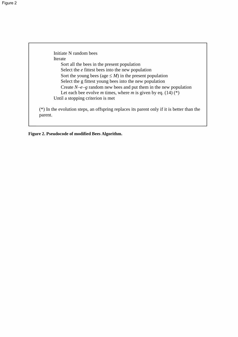
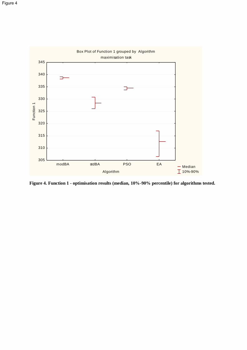
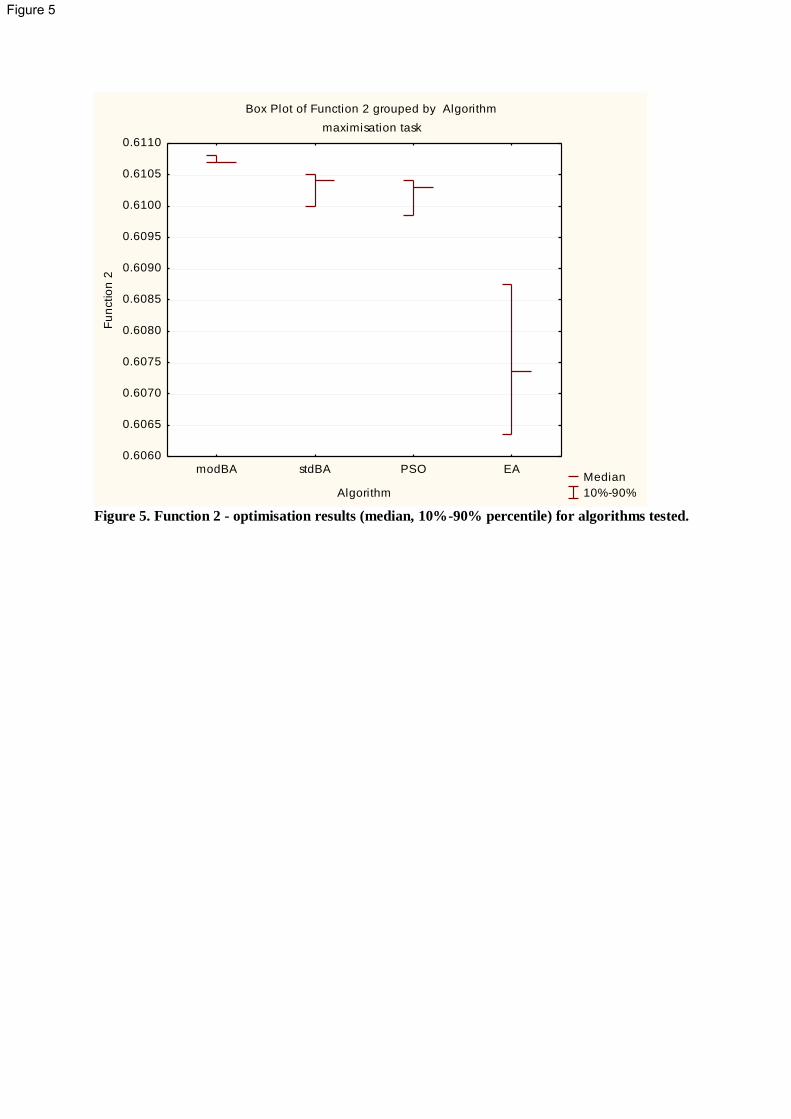
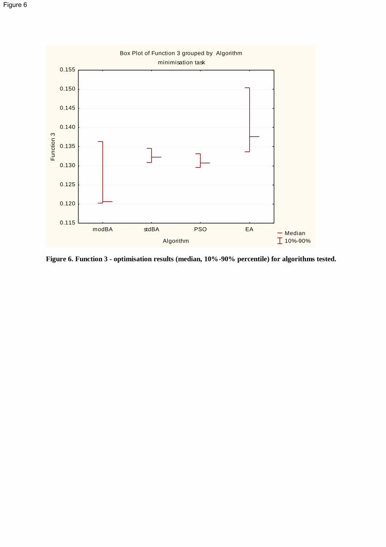
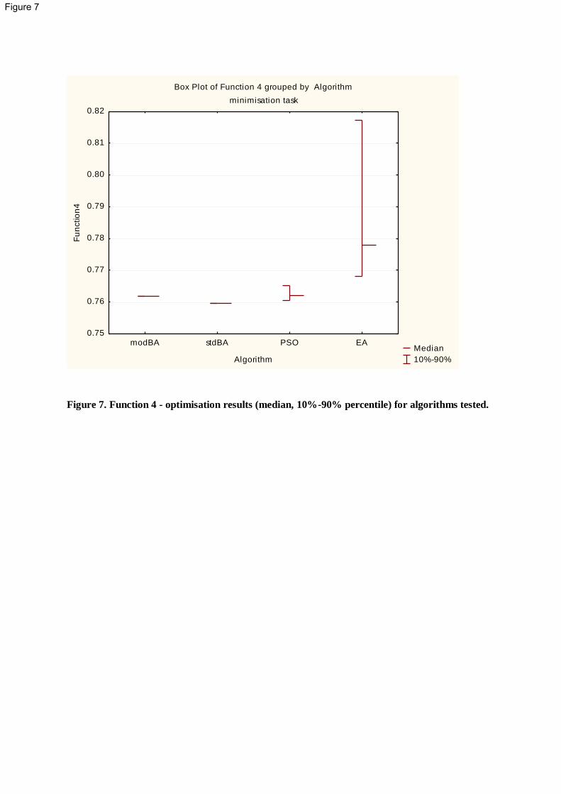
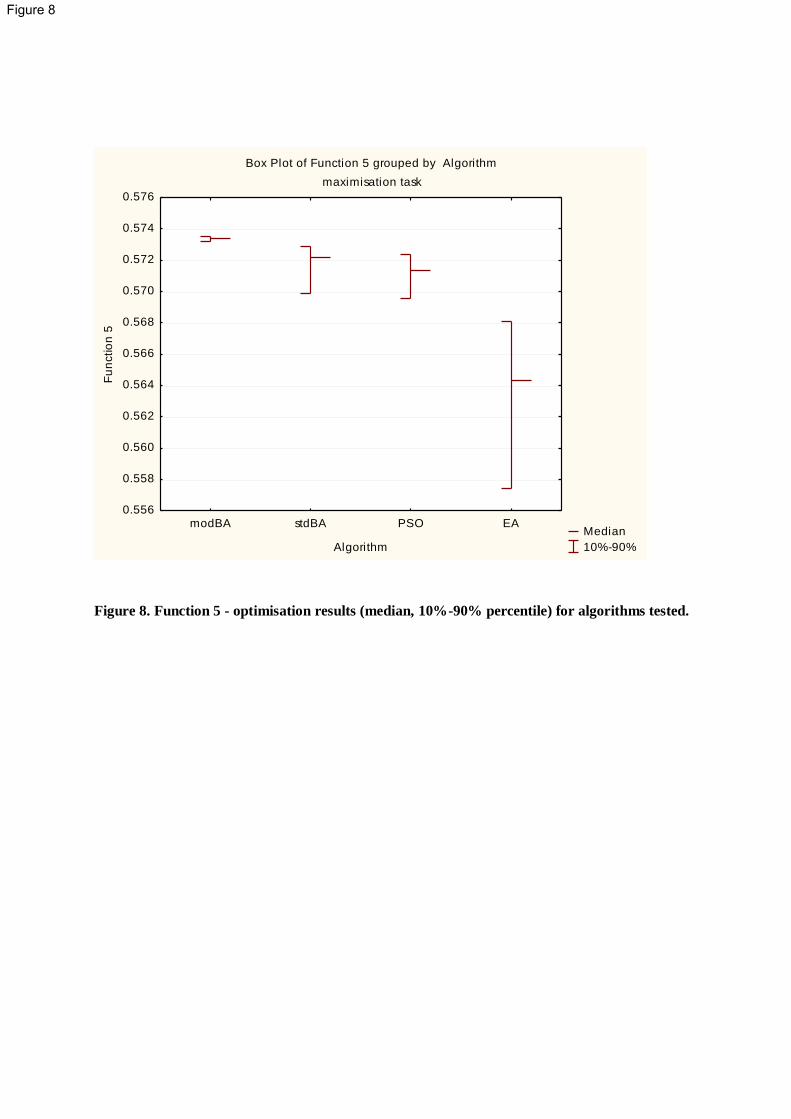
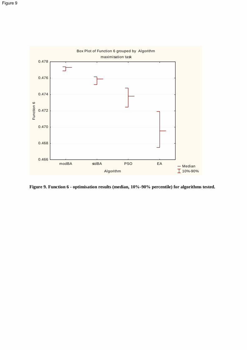
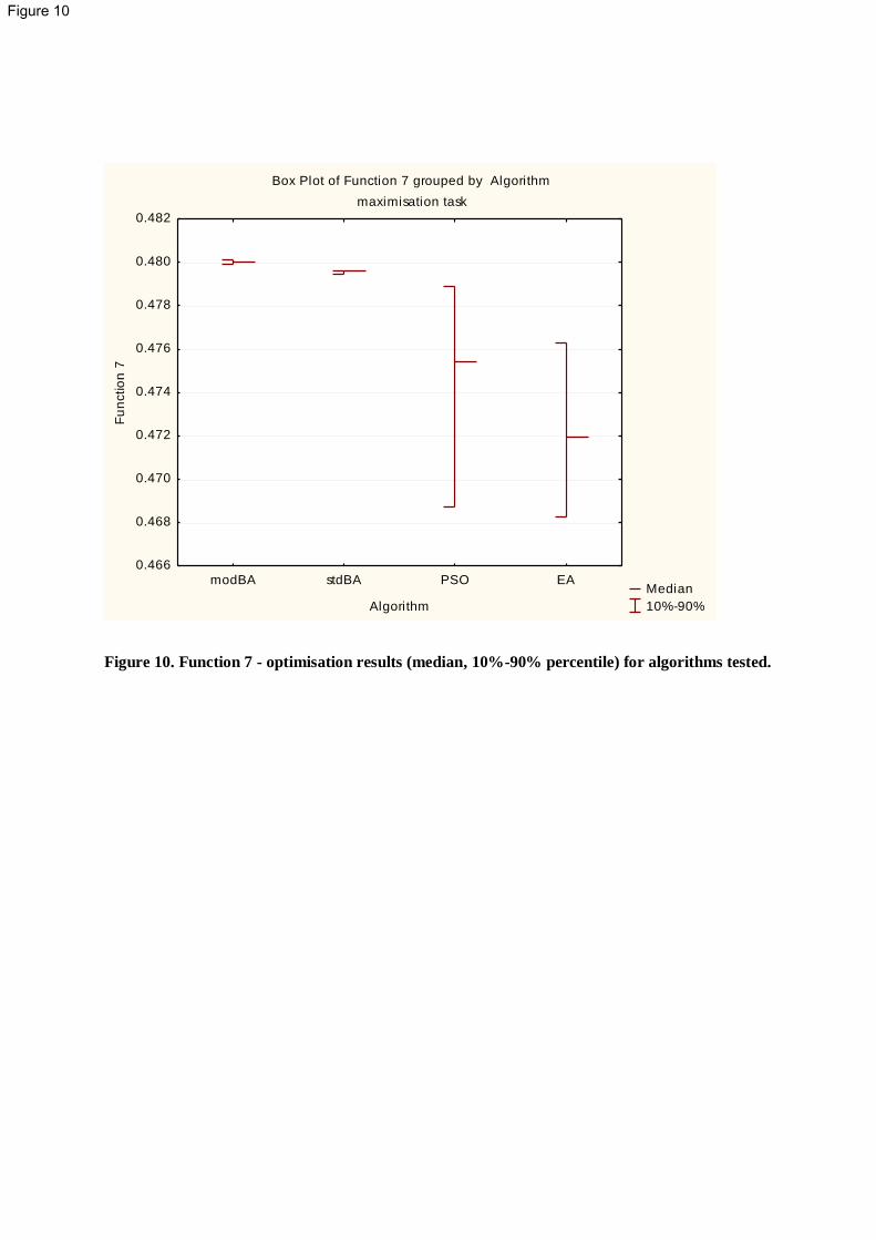
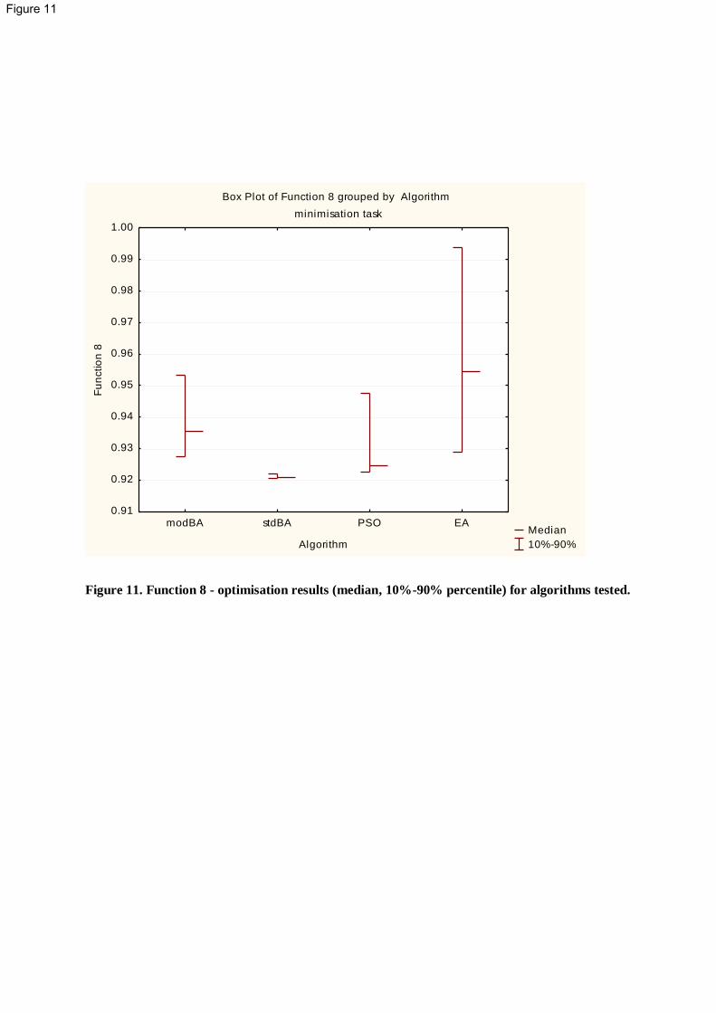
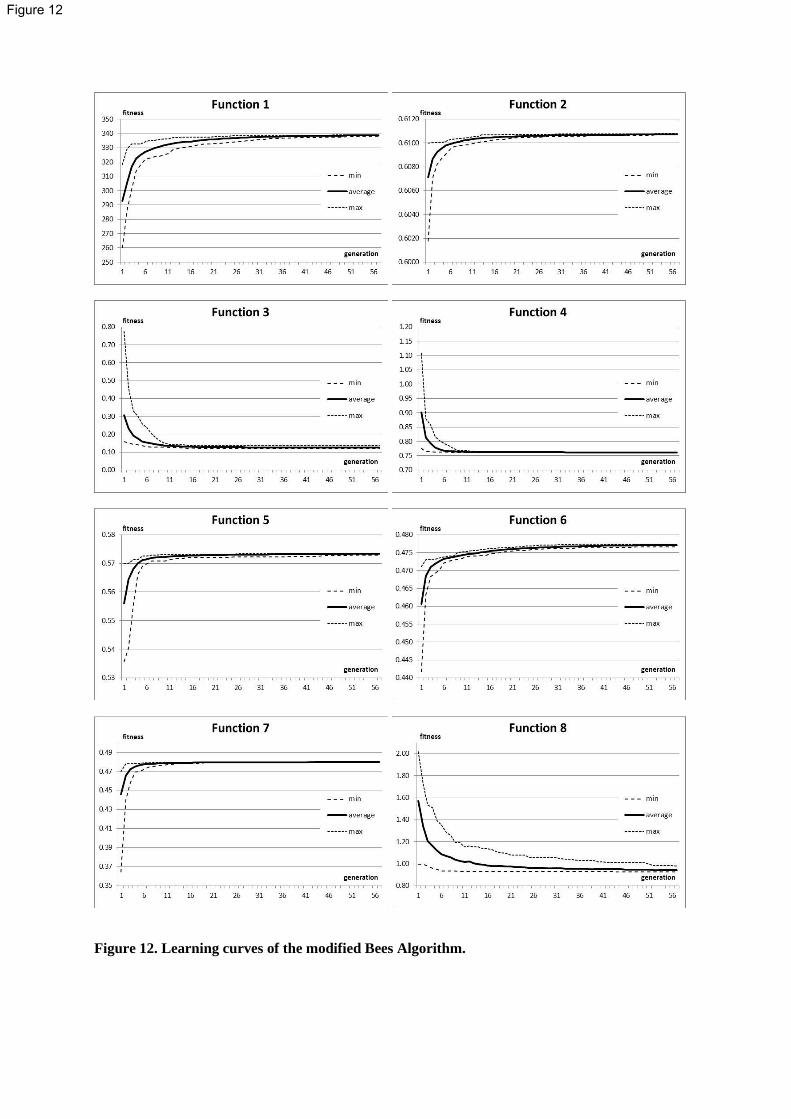
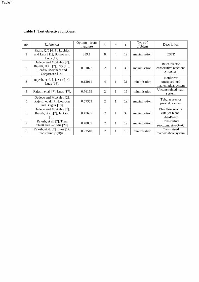
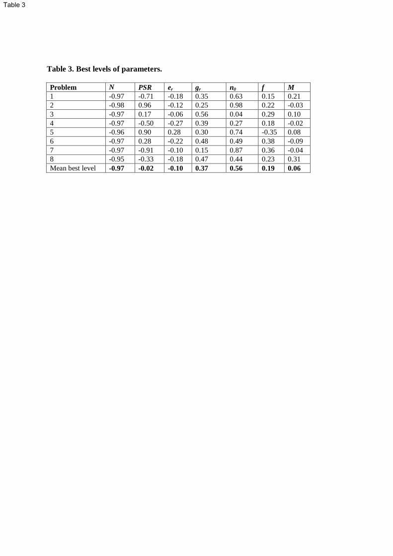
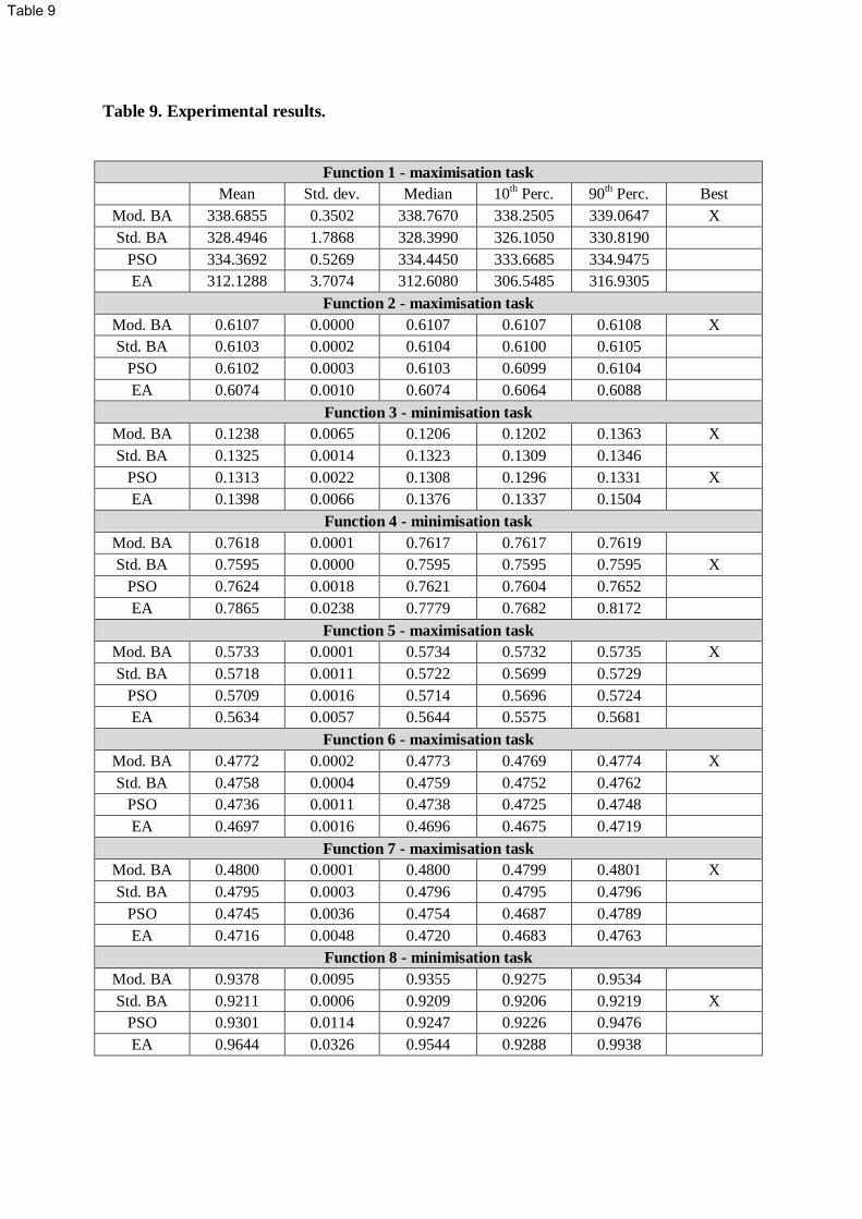


