arX

iv:c

ond-

mat

/050

4535

v3 [

cond

-mat

.sta

t-m

ech]

1 S

ep 2

005

Dynamical Exchanges in Facilitated Models of Supercooled Liquids

YounJoon Jung,1 Juan P. Garrahan,2 and David Chandler1

1Department of Chemistry, University of California, Berkeley, CA 94720-14602School of Physics and Astronomy, University of Nottingham, Nottingham, NG7 2RD, UK

(Dated: February 2, 2008)

We investigate statistics of dynamical exchange events in coarse–grained models of supercooledliquids in spatial dimensions d = 1, 2, and 3. The models, based upon the concept of dynamicalfacilitation, capture generic features of statistics of exchange times and persistence times. Here,distributions for both times are related, and calculated for cases of strong and fragile glass formersover a range of temperatures. Exchange time distributions are shown to be particularly sensitiveto the model parameters and dimensions, and exhibit more structured and richer behavior thanpersistence time distributions. Mean exchange times are shown to be Arrhenius, regardless of modelsand spatial dimensions. Specifically, 〈tx〉 ∼ c−2, with c being the excitation concentration. Differentdynamical exchange processes are identified and characterized from the underlying trajectories. Wediscuss experimental possibilities to test some of our theoretical findings.

I. INTRODUCTION

Dynamical arrest of liquids as they approach the glasstransition is a topic of much current research. [1, 2, 3, 4]This arrest entails such features as non–exponential re-laxation and precipitous non–Arrhenius temperature de-pendence of transport properties. At its heart lies thenotion of dynamic heterogeneity. [5, 6, 7, 8, 9, 10, 11, 12]Namely, as the temperature decreases towards the glasstransition, mobility develops spatial inhomogeneity, andas time progresses local mobility undergoes dynami-cal changes. We have interpreted these phenomena[13, 14, 15, 16, 17] in terms of local excitations of mobilityin space that propagate in time with facilitated dynam-ics. [18, 19, 20, 21] The excitations thus form lines inspace–time. Dynamic scaling is described naturally interms of the statistics of these lines. [13, 14, 22, 23]

The work we present in this paper is motivated by re-cent experiments that directly detect local fluctuationsof dynamics in supercooled liquids. [7, 9, 11, 12, 24]For example, single molecule rotational experiments [12]show that changes in local dynamics are similar to ran-dom telegraph noise, where local spatial regions exhibitdynamical exchanges between fast and slow dynamics.Similar stochastic behavior is also observed in local di-electric fluctuation experiments. [7] In those experimentsa local spatial region exhibits dynamical exchanges be-tween fast and slow dynamics, thus yielding direct con-firmation of dynamic heterogeneity.

Considering these experiments, we establish genericfeatures of statistical properties of dynamical exchangeevents and show how these features manifest themselvesin experimental observables. In the low temperatureregime, dynamics in supercooled liquids is dominated byfluctuations, not the mean. Therefore, it is pertinent tostudy the whole distribution in order to gain insights onthe microscopic nature of dynamics in supercooled liq-uids and glasses.

We do so in this paper in the context of coarse–grainedfacilitated models. In Sec. II, we define these models.

In Sec. III, we define exchange and persistence times,and derive an analytical relationship between the distri-butions of exchange and persistence times. In Sec. IV,qualitative features of the exchange time distribution arepresented. Numerical results of distributions of exchangeand persistence times for the models are described inSec. V. In Sec. VI we present results of numerical simula-tions of dynamic bleaching experiments. We conclude inSec. VII with discussions of possible experimental mea-surements aimed at testing our theoretical predictions.

II. MODELS OF GLASS FORMERS

We assume that a kinetically constrained model [13,14, 18, 20, 25] is obtained through coarse graining overa microscopic time scale δt (e.g., larger than the molec-ular vibrational time scale), and also over a microscopiclength scale δl (e.g., larger than the equilibrium corre-lation length). The dimensionless Hamiltonian for themodel is,

H =

N∑

i=1

ni, (ni = 0, 1). (1)

Here, ni refers to a state of lattice site i at xi, whereni = 1 coincides with lattice site being a spatially un-jammed region (i. e., carrying mobility), while ni = 0coincides with it being a jammed region (i. e., not car-rying mobility). We thus call ni the “mobility field”. Inspatial dimensions d = 1, 2, and 3, the lattice is linear,square, and cubic, respectively. The number of sites, N ,specifies the size of the system. From Eq. (1), thermo-dynamics is trivial, and the equilibrium concentration ofdefects or excitations is given by

c = 〈ni〉 =1

1 + exp(1/T ), (2)

where T is a reduced temperature.

2

The dynamics of these models obeys detailed balancewith local dynamical rules that depend on the configura-tion of the lattice site i as well as those of its neighbors.Namely,

ni(t) = 0k(+)i−−−→ ni(t + δt) = 1, (3)

ni(t) = 1k(−)i−−−→ ni(t + δt) = 0, (4)

where

k(+)i = e−1/T fi ({nx}) , (5)

k(−)i = fi ({nx}) . (6)

The function fi ({nx}) = fi(n1, n2, · · · , nN ) reflects dy-namical facilitation.

In the Fredrickson–Andersen (FA) model, [18] a changeof state at site i can occur from t to t+δt, ni(t+δt) = 1−ni(t), if at least one of 2d nearest neighbors of the ith siteis excited. For example, in d = 1 case, [18] ni(t + δt) =1 − ni(t) is allowed only if nj(t) = 1 where xj = xi ± δl.In contrast, in the d = 1 East model case, [20] one needsan excited neighbor in specific directions in order to havea state change at site i. For instance, nj(t) = 1 such thatxj = xi − δl.

In d = 3 cases, ni(t) at xi = (x, y, z) can make a changeif at least there is one nearest neighbor site j such thatnj(t) = 1 at xj = (x±δl, y, z) or (x, y±δl, z) or (x, y, z±δl) (FA model) or xj = (x − δl, y, z) or (x, y − δl, z) or(x, y, z − δl) (East model). The facilitation function forthe FA and East model, fi ({nx}), is therefore given by,

[fi ({nx})]FA = 1 −

d∏

l=1

(1 − nxi+δlul)(1 − nxi−δlul

),

(7)

[fi ({nx})]East = 1 −

d∏

l=1

(1 − nxi−δlul), (8)

where ul is a unit vector in the lth dimension. In the clas-sification scheme of kinetically constrained models givenin Ref. 25, these kinetic constraints correspond to one–spin facilitation rule in d dimension.

III. EXCHANGE AND PERSISTENCE TIMES

Relaxation time scales of the glassy systems can bedescribed by a distribution of persistence times, tp, thetime at which a local region changes its state for the firsttime once the trajectory has started at time zero. In thed = 1 FA model, for instance, the mean persistence timeexhibits Arrhenius behavior at low temperatures. [15]

A statistical measure which is useful in studyingchanges in dynamics of local environments is the distri-bution of exchange times, tx, the time duration of givenstates of mobility fields. For example, it has been shown

x

t

x

xp

tp

t

t

t

FIG. 1: Exchange and persistence times are shown in thetrajectory of d = 1 FA model at T = 0.8. Shaded regionsrepresents parts of space-time with excitations, while whiteregions represent parts with no excitations.

that the decoupling of the translational diffusion fromthe relaxation times in supercooled liquids near the glasstransition can be explained from the distribution of ex-change times. [16, 17] Persistence and exchange timesare illustrated in the trajectory of d = 1 FA model inFig. 1.

Exchange and persistence times are different statisti-cal measures of the same trajectories. There is a generalrelation between exchange and persistence time distribu-tions, independent of models. To derive the relation, wedefine the variable

Pi(t; 1, τ) =

[

t−δt∏

t′=0

ni(τ + t′)

]

[1 − ni(τ + t)] . (9)

It is the density of excitations at time τ (i.e., ni = 1)that persist until time t+ τ . A similar expression for thedensity of unexcited sites that persist for this time frame,Pi(t; 0, τ), is given by Eq. (9) with ni changed to 1 − ni,and 1 − ni changed to ni.

Similarly,

Xi(t; 1, τ) =1

δt[1 − ni(τ − δt)]

[

t−δt∏

t′=0

ni(τ + t′)

]

× [1 − ni(τ + t)] , (10)

is the density of excitations that exchange over the timeinterval between τ and t + τ . Clearly,

Xi(t; 1, τ) =1

δt[Pi(t; 1, τ) − Pi(t + δt; 1, τ − δt)] . (11)

Averaging and taking δt → 0+ therefore yields

X (t; 1) = −dP(t; 1)

dt, (12)

where X (t; 1) = 〈Xi(t; 1, τ)〉 and P(t; 1) = 〈Pi(t; 1, τ)〉.The normalized probability densities of exchange andpersistence times for an excitation, px(t; 1) and pp(t; 1),

3

respectively, are proportional to X (t; 1) and P(t; 1), re-spectively. Accounting for normalization constants there-fore gives

pp(t; 1) =

∫

∞

t dt′ px(t′; 1)

〈tx(1)〉, (13)

where 〈tx(1)〉 =∫

∞

0 dt tpx(t; 1) is the mean exchange timefor an excitation.

One can also proceed the same route for persistenceand exchange of no excitation by replacing ni with 1−ni

in Eqs. (9) and (10) to find

pp(t; 0) =

∫

∞

t dt′ px(t′; 0)

〈tx(0)〉. (14)

The overall exchange and persistence time probabilitydensities, px(t), and pp(t), are given by

px(t) =1

2[px(t; 0) + px(t; 1)] , (15)

pp(t) = (1 − c)pp(t; 0) + cpp(t; 1). (16)

Using Eqs. (13) and (14) with the condition of detailedbalance,

〈tx(1)〉

〈tx(0)〉=

c

1 − c, (17)

we find

pp(t) =

∫

∞

t dt′ px(t′)

〈tx〉, (18)

where 〈tx〉 = 12 (〈tx(0)〉 + 〈tx(1)〉). For a Poisson process,

which is valid for unconstrained dynamics, px(t; n) =τ(n)−1 exp(−t/τ(n)). In that case, the exchange andpersistence time distributions become identical to eachother. [26]

Moments of the two distributions are related to eachother from Eq. (18) through integration by parts. Inparticular,

〈(tp)m〉 =〈(tx)

m+1〉

(m + 1)!〈tx〉. (19)

The moments of the persistence time distributions arealways greater than those of the exchange time distribu-tions when the distributions are broader than Poissonian.Correlations between exchange events are described bycorrelation functions of the type

Cij(t, t′|n, τ, n′, τ ′) = 〈δXi(t; n, τ)δXj(t

′; n′, τ ′)〉, (20)

where δXi(t; n, τ) ≡ Xi(t; n, τ) −X (t; n).

IV. ANALYSIS OF EXCHANGE TIME

DISTRIBUTIONS

We have calculated exchange and persistence time dis-tributions for the FA and East models by performing

-2 0 2 40

0.2

0.4

0.6

Px(l

og10

t) a

nd P

p(log

10t)

-2 0 2 4log

10 t

0

0.2

0.4

0.6

-2 0 2 40

0.2

0.4

0.6

-2 0 2 4 6log

10 t

0

0.2

0.4

0.6

(a)

(c)

(b)

(d)

FIG. 2: Exchange and persistence time distributions for d = 1FA and East models. Here, Px(log10 t) = tpx(t) ln(10), andPp(log10 t) is similarly related to pp(t). Exchange time dis-tribution from simulation (filled circles), persistence time dis-tribution from simulation (open circles), and persistence timedistribution predicted from Eq. (18) (solid lines). (a) d = 1FA model at T = 1, (b) d = 1 FA model at T = 0.5, (c) d = 1East model at T = 1, and (d) d = 1 East model at T = 0.5.

Monte Carlo simulations. For the purpose of numeri-cal efficiency, we have used the continuous time MonteCarlo algorithm. [27, 28] To sample long exchange times(i.e., log10 tx > 1), we have used N = 100c−1. To sam-ple short exchange times (i.e., log10 tx < 1), we haveused N = 105c−1. The two distributions obtained werematched at log10 tx = 1. Simulations were performed fortotal times T = 500 τα, with τα being the relaxationtime of the model. Averages were performed on about100 independent trajectories in each case.

As an illustration, we show in Fig. 2 exchange andpersistence time distributions obtained from numericalsimulations, and compare those results with the predic-tion of Eq. (18). The comparison verifies Eq. (18). Thepeak and principal statistical weight in the persistencetime distribution occurs at a longer time than that forthe exchange time distribution.

A. Moments of Exchange and Persistence Times

In many experiments, measurements of moments offluctuating quantities are more easily made than mea-surements of the whole distributions. Studies of mo-ments will yield information on underlying dynamics.[29, 30] We have studied temperature dependence of themoments of exchange and persistence time distributions,〈(tx)

m〉 and 〈(tp)m〉 (m=1, 2, and 3), respectively, of the

4

100

101

102

103

100

105

1010

1015

1020

1025

100

101

102

100

105

1010

1015

1020

1025

100

101

102

103

100

105

1010

1015

<tm

>

100

101

102

100

105

1010

1015

1020

1025

100

101

102

103

1/c

100

105

1010

1015

100

101

102

1/c

100

105

1010

1015

1020

d=1d=1

d=2 d=2

d=3d=3

m=3

m=2

m=1

FA models East models

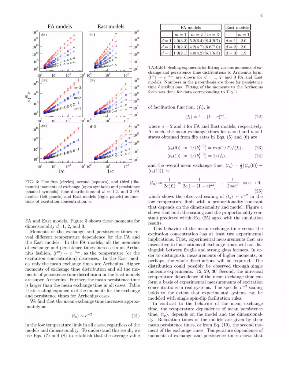
FIG. 3: The first (circles), second (squares), and third (dia-monds) moments of exchange (open symbols) and persistence(shaded symbols) time distributions of d = 1,2, and 3 FAmodels (left panels) and East models (right panels) as func-tions of excitation concentration, c.

FA and East models. Figure 3 shows these moments fordimensionality d=1, 2, and 3.

Moments of the exchange and persistence times re-veal different temperature dependence for the FA andthe East models. In the FA models, all the momentsof exchange and persistence times increase in an Arrhe-nius fashion, 〈tm〉 ∼ c−αm , as the temperature (or theexcitation concentration) decreases. In the East mod-els only the mean exchange times are Arrhenius. Highermoments of exchange time distribution and all the mo-ments of persistence time distribution in the East modelsare super–Arrhenius. Further, the mean persistence timeis larger than the mean exchange time in all cases. TableI lists scaling exponents of the moments for the exchangeand persistence times for Arrhenius cases.

We find that the mean exchange time increases approx-imately as

〈tx〉 ∼ c−2, (21)

in the low temperature limit in all cases, regardless of themodels and dimensionality. To understand this result, weuse Eqs. (7) and (8) to establish that the average value

FA models

m = 1 m = 2 m = 3

d = 1 2.0(3.2) 5.2(6.4) 8.4(9.7)

d = 2 1.9(2.3) 4.2(4.7) 6.6(7.0)

d = 3 1.9(2.1) 4.0(4.2) 6.1(6.3)

East models

m = 1

d = 1 2.0

d = 2 2.0

d = 3 1.9

TABLE I: Scaling exponents for fitting various moments of ex-change and persistence time distributions to Arrhenius form,〈tm〉 ∼ c−αm are shown for d = 1, 2, and 3 FA and Eastmodels. Numbers in the parenthesis are those for persistencetime distributions. Fitting of the moments to the Arrheniusform was done for data corresponding to T ≤ 1.

of facilitation function, 〈fi〉, is

〈fi〉 = 1 − (1 − c)ad, (22)

where a = 2 and 1 for FA and East models, respectively.As such, the mean exchange times for n = 0 and n = 1states obtained from flip rates in Eqs. (5) and (6) are

〈tx(0)〉 ≈ 1/〈k(+)i 〉 = exp(1/T )/〈fi〉, (23)

〈tx(1)〉 ≈ 1/〈k(−)i 〉 = 1/〈fi〉, (24)

and the overall mean exchange time, 〈tx〉 = 12 (〈tx(0)〉 +

〈tx(1)〉), is

〈tx〉 ≈1

2c〈fi〉=

1

2c[1 − (1 − c)ad]→

1

2adc2, as c → 0,

(25)which shows the observed scaling of 〈tx〉 ∼ c−2 in thelow temperature limit with a proportionality constantthat depends on the dimensionality and model. Figure 4shows that both the scaling and the proportionality con-stant predicted within Eq. (25) agree with the simulationresults.

This behavior of the mean exchange time versus theexcitation concentration has at least two experimentalimplications. First, experimental measurements that areinsensitive to fluctuations of exchange times will not dis-tinguish between fragile and strong glass formers. In or-der to distinguish, measurements of higher moments, orperhaps, the whole distributions will be required. Thedistribution could possibly be observed through singlemolecule experiments. [12, 29, 30] Second, the universaltemperature dependence of the mean exchange time canform a basis of experimental measurements of excitationconcentrations in real systems. The specific c−2 scalingholds to the extent that experimental systems can bemodeled with single spin-flip facilitation rules.

In contrast to the behavior of the mean exchangetime, the temperature dependence of mean persistencetime, 〈tp〉, depends on the model and the dimensional-ity. Relaxation times of the models are given by theirmean persistence times, or from Eq. (19), the second mo-ment of the exchange times. Temperature dependence ofmoments of exchange and persistence times shows that

5

1 10 100 10001/c

100

101

102

103

104

105

106

2ad

<t x>

d=1 FAd=2 FAd=3 FAd=1 Eastd=2 Eastd=3 East

(1/c)2

FIG. 4: Comparison of mean–field approximation, Eq. (25)(dashed line), and simulation results of mean exchange timesin d = 1, 2, and 3 FA and East models. a = 2 for FA modelsand a = 1 for East models.

relaxation times are Arrhenius for the FA models andsuper-Arrhenius for the East models.

As the dimensionality of the model increases, differ-ences between the moments of exchange and persistencetimes become smaller in the FA model. The model be-comes increasingly mean–field like in higher dimensions.No such convergence is found in the East model for alldimensions investigated. The East models have weak di-mensional dependence due to the quasi-one dimensionalnature of directional persistence.

B. Stokes–Einstein Breakdown

For the FA models, which correspond to strong glassformers, the translational diffusion constant scales as [16]

DFA ∼ 〈tx〉−1 ∼ c2. (26)

This result is true in all dimensions. It follows fromEq. (21) and the statement that adjacent random walksteps coincide with adjacent exchange events. For theEast models, however, the result does not hold becauseadjacent exchange events are correlated. In particular,for the hierarchical dynamics of the East models, largebubbles in space-time are covered with smaller bubbles,which in turn are covered by yet smaller bubbles, and soon. [13] In that case, higher moments of exchange timedistributions exhibit different temperature dependencefrom that of the mean. This behavior is illustrated in

Fig. 3 for the East model, which corresponds to a fragileliquid. Correlations between successive exchange eventscan be investigated by using correlation function givenin Eq. (20). The effects are responsible for non–trivialscaling relation between the translational diffusion andpersistence times in fragile liquids. [16, 31, 35, 36, 37, 38]

Indeed, numerical results for the fractional Stokes-Einstein relationship,

D ∝ τ−ξα (27)

give ξ ≈ 2/3, 2/2.3, 2/2.1 for dimensions d = 1, 2, 3 in thecase of the FA models, while ξ ≈ 0.7 − 0.8 (very weaklydependent on d) in the case of the East models. [16, 31]

C. Classifications of Exchange Events

We show in Fig. 5 representative exchange time distri-butions. At short exchange times, log10 tx < −1, the dis-tribution Px(log10 tx) follows a power-law behavior witha slope 1 in all cases, Px(log10 tx) ∼ log10 tx. This is be-cause Px(log10 tx) ∼ txpx(tx), and Poissonian statistics isobeyed, px(tx) ∼ exp(−tx), for short times.

Multiple peak structures develop in the exchange timedistributions at low temperature. In order to investigatethe structure of exchange time distributions in detail, wedefine mobility index, mi(t), that depends upon whetherthe lattice site is filled with an excitation or not andalso whether it is in an mobile or immobile configuration.Specifically,

mi(t) = 4 − 2ni(t) − fi(t), (28)

where fi(t) = 1 when the lattice site i is in a mobileconfiguration at time t, and it is zero otherwise. As such,mi(t) is 1 when site i is excited and mobile, 2 when it isexcited and immobile, 3 when it unexcited and mobile,and 4 when it is unexcited and immobile.

During an exchange time of the lattice site i, ni doesnot change, while its nearest neighbors may make flippingevents, thus changing mi over time. In order to monitorchanges in the local mobility during an exchange time,it is useful to introduce an averaged mobility index for asingle exchange event,

mi(ts) =1

tx

∫ tx

0

dt′mi(ts + t′), (29)

where ts is the start time of an exchange event for sitei, and the zero time in this formula is the time at whichthe exchange event begins. See Fig. 1. If there has notbeen any change in the local configuration during an ex-change time, the lattice site remains always mobile, andthe averaged mobility index will be either mi = 1 (forni = 1) or mi = 3 (for ni = 0). However, when the localmobility changes during the exchange time period due tochanges of the states in nearest neighbors, the averagedmobility index will be either 1 < mi < 2 (for ni = 1) or

6

-2 0 2 4 610-4

10-3

10-2

10-1

100

-2 0 2 4 610-4

10-3

10-2

10-1

100

-2 0 2 410-4

10-3

10-2

10-1

100

Px(l

og10

t x)

-2 0 2 4 610-4

10-3

10-2

10-1

100

-2 0 2 4log

10tx

10-4

10-3

10-2

10-1

100

-2 0 2 4log

10tx

10-4

10-3

10-2

10-1

100

d=1 d=1

d=2d=2

d=3 d=3t0* t

2*t

1*

FA models East models

FIG. 5: Decompositions of exchange time distributions of FAmodels (left panels) and East models (right panels) for d =1,2, and 3 at T = 0.3. Four sub-distributions – case 1 (circles),case 2 (squares), case 3 (diamonds), and case 4 (triangles) -add up to the full distribution (solid line). Positions of threepeaks in P (log10 tx) are shown for d = 3 FA model cases.

3 < mi < 4 (for ni = 0). We define four different casesof the averaged mobility. Namely,

case 1 : mi = 1 (ni = 1 and fi = 1)

case 2 : 1 < mi < 2 (ni = 1 and fi changes)

case 3 : mi = 3 (ni = 0 and fi = 1)

case 4 : 3 < mi < 4 (ni = 0 and fi changes).

(30)

Examples of exchange times that belong to each case areshown in the trajectory picture of d = 1 FA model inFig. 6.

To illustrate the correlation between exchange timesand environments, Fig. 5 shows exchange time distribu-tions and their sub-distributions, each corresponding toone of the cases in Eq. (30), for d = 1, 2, and 3 FA andEast models at T = 0.3. There exist multiple peaks inthe distributions of exchange times at low temperaturein all the cases shown in Fig. 5. Positions of peaks inthe distribution, t∗0, t∗1, and t∗2, are shown in the caseof d = 3 FA model. Temperature dependence of thesepeaks for d = 1, 2, and 3 FA and East models are pre-

case 4

case 1

case 3case 2

FIG. 6: Examples of exchange events that belong to each caseof Eq. (30) are illustrated in the trajectory of d = 1 FA model.

100

101

102

103

100

101

102

100

101

102

100

101

102

103

100

101

102

103

100

102

104

106

t*

100

101

102

100

101

102

103

104

100

101

102

103

1/c

100

102

104

100

101

102

1/c

100

101

102

103

104

d=1d=1

d=2 d=2

d=3d=3

t0*

t1*

t2*

FA models East models

FIG. 7: Positions of peaks in the exchange time distributionsare shown for various excitation concentrations.

sented in Fig. 7, and in all the cases, each peak positionis Arrhenius,

t∗n ∼ c−n (31)

where n = 0, 1, and 2.To reveal the physical origins of each peak in the ex-

change time distributions, the temperature dependenceof each peak in the exchange time distribution is shown

7

in Fig. 7. Cases 1 and 2 will involve disappearances of ex-citations, while cases 3 and 4 appearances of excitationsin the trajectory space. The first peak in the exchangetime distribution corresponds to fast processes of mobilen = 1 states embedded in the excitation line. In this case,the excited state will quickly de-excite in time t∗0 ∼ c0,and the position of the first peak in the exchange time dis-tribution does not depend on the temperature as shownin Fig. 7. This process will have the averaged mobilityindex, m = 1, corresponding to case 1 in Eq. (30).

The mobile region located at the boundary of excita-tion line will have a probability of becoming immobiledue to changes in its nearest neighbors and becomingmobile later. This process corresponds to case 2 withthe averaged mobility index 1 < m < 2. It is respon-sible for fluctuations of thicknesses of excitation lines intrajectory space, and it gives rise to the second peak inthe exchange time distribution, with temperature depen-dence t∗1 ∼ c−1.

Dynamical exchange processes corresponding to case 3also contribute to the second peak in the distribution. Inthis case, n = 0 state next to an excitation line becomesexcited in time t∗1 ∼ c−1. This process involves a creationof an excitation next to a pre-existing excitation line. Interms of the geometry of the trajectory space, exchangeevents corresponding to cases 2 and 3 are responsible forbending of excitation lines.

Finally, the exchange events that have the longesttimes, resulting in the third peak, will correspond to theup-flip event of the n = 0 states far away from the exci-tation lines. This case has the averaged mobility indexof case 4. In d = 1 FA model, for example, it corre-sponds to a region deep inside the bubble structure inthe trajectory space.

V. DISTRIBUTIONS OF EXCHANGE AND

PERSISTENCE TIMES

A. Strong Glass Former Models

Figure 8 compares the exchange time distributions (leftpanels) and persistence time distributions (right panels)for d = 1,2, and 3 FA models at various temperatures.Exchange time distributions shown in the left panel de-pend strongly on the temperature. In the high tempera-ture regime, the exchange time distribution has a singlepeak because there is no clear distinction between dif-ferent exchange events due to the mean-field nature ofthe dynamics in the high temperature regime. However,as temperature decreases, the mean-field picture is nolonger valid, excitation lines dominate trajectory space,and different kinds of dynamical exchange events mani-fest themselves in the distribution as distinct peaks. Thisfact is evident from the multiple peak structures in theexchange time distribution in all dimensions in the FAmodel. In d = 3 FA model, for instance, distinct tripletstructure is observed when T = 0.4 and below. Each peak

-2 0 2 4 60

0.2

0.4

0.6

0.8

-2 0 2 4 6 80

0.2

0.4

0.6

0.8

-2 0 2 4 60

0.2

0.4

0.6

0.8

Px(l

og10

t x)

-2 0 2 4 60

0.2

0.4

0.6

0.8

Pp(l

og10

t p)

-2 0 2 4 6log

10tx

0

0.2

0.4

0.6

0.8

-2 0 2 4 6log

10tp

0

0.2

0.4

0.6

0.8

d=1 d=1

d=2d=2

d=3 d=3

Exchange times Persistence times

FIG. 8: Distributions of the logarithm of exchange and per-sistence times of FA model for d = 1,2, and 3 at varioustemperatures. From left to the right: T = 10, 1, 0.55, 0.4,0.3, 0.22, 0.18 for d = 1 case, and T = 10, 1, 0.55, 0.4, 0.3,0.22, 0.18, 0.16 for d = 2 and d = 3 cases.

corresponding to different dynamical exchange event ex-hibits different behaviors of temperature dependence aspresented in Fig. 7.

As the dimensionality increases, the exchange time dis-tribution shows more and more well–separated tripletpeak structure in the low temperature regime. The rela-tive weight of the third peak increases as the dimension-ality increases.

The persistence time distributions shown in the rightpanel of Fig. 8 are less structured than the exchange timedistributions, as to be expected from Eq. (18). As thetemperature decreases, the single peak in the persistencetime distribution moves towards the long time region.Physically, persistence time distributions are statisticalmeasures of duration of a state at an arbitrary space-timepoint in the trajectory space. Thus, relative to exchangetime distributions, persistence time distributions empha-size processes occurring over longest times. The greaterstructure in the exchange time distributions, relative tothe persistence time distributions, is due to the formergiving equal weights to events, irrespective of their dura-tions.

8

-2 0 2 40

0.2

0.4

0.6

-2 0 2 4 6 80

0.2

0.4

0.6

-2 0 2 40

0.2

0.4

0.6

0.8

Px(l

og10

t x)

-2 0 2 4 6 80

0.2

0.4

0.6

0.8

Pp(l

og10

t p)

-2 0 2 4log

10tx

0

0.2

0.4

0.6

0.8

-2 0 2 4 6 8

log10

tp

0

0.2

0.4

0.6

0.8

d=1 d=1

d=2d=2

d=3 d=3

Exchange times Persistence times

FIG. 9: Distributions of the logarithm of exchange and per-sistence times of East model for d = 1, 2, and 3 at varioustemperatures. From left to the right: T = 10, 1, 0.6, 0.5, 0.4,and 0.3 for d = 1 case, T=10, 1, 0.5, 0.4, 0.3, 0.25, and 0.22for d = 2 case, and T=10, 1, 0.5, 0.4, 0.3, 0.25, 0.22, and 0.2for d = 3 case.

B. Fragile Glass Former Models

Exchange and persistence time distributions for theEast model cases are shown in Fig. 9. In the high tem-perature regime, the exchange time distributions have asingle peak as in strong liquids or FA models. However,in the low temperature regime, in contrast with its be-havior in the FA model, they show two dominant doubletpeaks in all dimensions. We also notice that, albeit small,broad tails develop in the wings of the distributions atlow temperatures. This feature is especially evident inFig. 10, where the exchange time distributions of the FAand East models are compared in log–log scale. In thecase of persistence time distributions shown in the rightpanel of Fig. 9, single peaks develop into broad distribu-tions with shoulders as temperature decreases.

We compare exchange time distributions in FA andEast models in Fig. 10. In d = 1 case, exchange time dis-tributions of both FA and East models show long timetails in the low temperature regime in common. Addi-tionally, the distributions in the East model exhibit log-arithmic oscillations. In higher dimensions, d = 2 and

-2 0 2 4 6 810-4

10-3

10-2

10-1

100

-2 0 2 4 6 10-5

10-4

10-3

10-2

10-1

100

-2 0 2 4 610-4

10-3

10-2

10-1

100

Px(l

og10

t x)

-2 0 2 4 6 10-4

10-3

10-2

10-1

100

-2 0 2 4 6log

10tx

10-4

10-3

10-2

10-1

100

-2 0 2 4 6log

10tx

10-4

10-3

10-2

10-1

100

d=1 d=1

d=2d=2

d=3 d=3

FA models East models

FIG. 10: Exchange time distributions of FA models (leftpanels) and East models (right panels) in log scales. Tem-peratures are the same as those given in the captions toFigs. 8 and 9. A power-law corresponding to px(tx) ∼ t−α

x

or Px(log10 tx) ∼ txpx(tx) ∼ t1−αx is shown as a dashed line

with α = 0.52, and a stretched exponential corresponding to

px(tx) ∼ e−(tx)β

where β = 0.38 is shown as a dot–dashed linefor d = 1 FA model. In d = 2 and 3 FA models, exponentialfits, px(tx) ∼ e−tx/τ , are given as dashed lines for the lowesttemperature of each case.

3, the exchange time distributions in FA models exhibitdistinct multiplet peak structures due to their mean-fieldnatures in higher dimensions. However, the distributionsin the East models remain similar to those in d = 1 cases,exhibiting long time tails and superimposed logarithmicoscillations. These are due to the hierarchical dynamicsthat arises from directed facilitation in the East modelsat all dimensions.

In the d = 1 FA case, due to the formations of bubble-like structures in the trajectory space, the exchange timedistributions decay with slowly decaying long time tails.It turns out that in d = 1 FA model case the exchangetime distribution first decays as a power-law (dashed line)then turns into a stretched exponential (dot–dashed line)as shown in Fig. 10. However, in d = 2 and d = 3 FAmodels, they decay as an exponential at the long time re-gion shown as dashed lines. This indicates that in higher

9

-2 0 2 4 6 8

log10

t

0

0.2

0.4

0.6

Pp(l

og10

t) -2 0 2 4 6 8 10log

10t

0

0.2

0.4

0.6

0.8

1

blea

chin

g ef

fici

ency

, φ(t

)

T=10

T=0.3

FIG. 11: Persistence time PDF’s at a high (T = 10) and alow (T = 0.3) temperature at equilibrium (solid lines) andright after the bleaching (dotted lines). Each dashed line cor-responds to the distribution created by bleaching efficiencyfunction, φ(t) with different values of τ , given in the insetof Fig. (11). Inset: Bleaching efficiency function used in thesimulation, Eq. (32), with α = 0.08. From left to the right, τprogressively increases from τ = 10−6 to τ = 106 by a factorof 100.

dimensions the FA models are less “glassy” than d = 1case. In higher dimensions, chances of forming bubble–like structures will be much smaller than in d = 1 case.In the East model cases, similar behaviors are observedin all dimensions. Namely, the exchange time distribu-tions decay with multiple transitions superimposed withstretched exponentials in the low temperature regime.

VI. SIMULATIONS OF BLEACHING

EXPERIMENTS

Experiments have been performed in order to mea-sure the timescale of the approach of non–equilibriumdistributions of local relaxation times to equilibrium.[9, 32, 33, 34] The timescale at which the non–equilibriumdistribution approaches to equilibrium will be called therecovery time. Based on the d = 1 East model, we presentresults of numerical simulations of one of such experi-ments - dynamical hole burning experiments or bleachingexperiments. [9, 32]

In numerical simulations of the bleaching experiment,the bleaching efficiency function, φ(t), is introduced as aprobability of bleaching out the region that has a localpersistence time of t. We choose the following form asφ(t),

φ(t) = min [1, (τ/t)α] , (32)

where τ and α can be varied. We choose τ = 1, and α =0.08 motivated by experimental results in Ref. 32. After alattice site is chosen to be “bleached out” in simulations,

0 0.2 0.4 0.6 0.8 1B

1

2

3

4

t obs(0

)/<

t p>

T=10T=1T=0.6T=0.3

FIG. 12: Mean persistence times right after the bleaching ex-periment, tobs(0), are shown for various bleaching depths andtemperatures. tobs(0) increases more abruptly as a functionof the bleach depth at a lower temperature.

persistence times of that site are not collected at latertimes as time goes on.

Numerical values of the bleaching efficiency functionsare shown in the inset of Fig. 11. The bleaching depth, B,is defined as the fraction of lattice sites that are bleachedout by applying the bleaching efficiency function, and isgiven by

B =

∫

∞

0

dtφ(t)pp(t). (33)

Probability distributions of persistence times after thebleaching are shown in Fig. 11 for two different values ofthe temperature and various values of τ .

Immediately after the bleaching, the system is out ofequilibrium, with a non-equilibrium persistence time dis-tribution given (to within a normalization constant) by

pne(t) =pp(t)(1 − φ(t))

1 − B. (34)

After waiting a time tw, this distribution relaxes top(t; tw), where p(t; 0) is pne(t) and p(t;∞) is the equi-librium pp(t). tobs(tw) is the first moment of p(t; tw),

tobs(tw) =

∫

∞

0

dt t p(t; tw), (35)

and tobs(0) > 〈tp〉. tobs(0) at various bleaching depthsand temperatures are shown in Fig. 12.

The relaxation dynamics is monitored by following atime evolution of the non–equilibrium persistence timedistribution obtained from un-bleached lattice sites forvarious waiting times, tw. Figure 13 shows the relax-ation dynamics of the initial non–equilibrium distribu-tion of persistence times for d = 1 East model at a lowtemperature.

10

-2 0 2 4 6log

10 t

0

0.1

0.2

0.3

0.4

0.5

P(lo

g 10 t;t

w)

tw

/<tp> = 0

2∞

FIG. 13: Relaxation dynamics of the distributions of persis-tence times to equilibrium after the bleaching of d = 1 Eastmodel at T = 0.5. τ = 1 and α = 0.08 were chosen in φ(t).

The timescale of the relaxation process of the non–equilibrium distribution can be estimated by severalmeans. For example, one can look at the waiting timedependence of moments of the distributions. Also, it ispossible to measure how far a non–equilibrium distribu-tion is separated from equilibrium by defining a distancebetween two distributions by

∆(tw) ≡

∫

∞

0

dt |p(t; tw) − pp(t)| . (36)

∆(tw) and the first three moments of the non–equilibriumdistribution are shown in Fig. 14 for different values ofthe waiting time. From these calculations, the timescaleof a recovery to equilibrium is estimated to be on the or-der of the equilibrium mean persistence time, 〈tp〉. Thispredication is at variance with results from bleaching ex-periments, [9, 32] but is is consistent with results fromNMR experiments. [33, 34, 39] The reason(s) for thisdiscrepancy remains to be clarified.

VII. DISCUSSION

In this paper, we have provided detailed illustrationsof the generally large differences between distributions ofpersistence times and exchange times. The distributionsare the same only when these distributions are Poisso-nian. Thus, the differences are manifestations of dynamiccorrelations, correlations that exist due to dynamic het-erogeneity. Despite the differences between the two dis-tributions, the behavior of one determines the other, asEq. (18) shows.

The first moment of the exchange time distributionis Arrhenius, independent of model and dimensional-ity. This result can be important if an experimental

0

0.1

0.2

0.3

∆(t w

)

0 5 10 15 20

tw

/<tp>

1

1.2

1.4

Rm

(tw

)

m=1m=2m=3

FIG. 14: Recovery of the non–equilibrium distribution,p(t; tw) to equilibrium is shown by the decay of ∆(tw) (up-per panel) and Rm(tw) ≡ 〈(tobs(tw))m〉/〈(tp)m〉 (lower panel).Timescale of the recovery to equilibrium is on the order of theequilibrium mean persistence time itself. The model parame-ters are the same as those used in Fig. 13.

means is available to measure this moment. In partic-ular, Eq. 21 shows that the measurement of the meanexchange time determines the average mobility concen-tration, c, the central control parameter in our descrip-tion of glassy dynamics. [13, 14, 15, 16, 17] This can beaccomplished with single-molecule experiments in whichexchange times for a probe molecule passing between fastand slow environments are measured directly. [12] Thedetermination of c in principle enables parameter-freetests of scaling relations we have predicted for transportproperties.

Significant experimental manifestations of the dif-ferences between exchange-time distributions andpersistence-time distributions are decoupling of differentmeasures of dynamics. The breakdown in Stokes–Einstein relations discussed in this paper is one example.Another is the existence of the Fickian crossover,marking the coarse-graining length-scale beyond whichrandom-walk diffusion is correct. [17] At large wave-vectors, dynamics is dominated by persistence andmolecular motion is not Fickian. At small wave-vectors,dynamics is dominated by exchange, and molecularmotion is Fickian.

Thus, there are many different relaxation times forslow dynamics in a glass former. Those connected tothe mean exchange time will be Arrhenius, even for frag-ile glass formers. Non-Arrhenius behavior (i.e., fragility),when it exists, is described by the second and higher mo-ments of the exchange-time distribution. This feature ofdynamics in glass formers is general, not a consequenceof a particular model. It follows from the presence ofdynamic heterogeneity and its consequential fluctuationdominance of dynamics.

11

Acknowledgment

We are grateful to M.D. Ediger, D.A. Vanden Bout,and A. Heuer for useful discussions. This work was sup-ported at Berkeley by the Miller Research Institute for

Basic Research in Sciences (YJ) and by the US Depart-ment of Energy Grant No. DE-FG03-87ER13793 (DC),and at Nottingham by EPSRC grants no. GR/R83712/01and GR/S54074/01 and University of Nottingham grantno. FEF 3024 (JPG).

[1] M. D. Ediger, C. Angell, and S. Nagel, J. Phys. Chem.100, 13200 (1996).

[2] C. A. Angell, Science 267, 1924 (1995).[3] P. G. Debenedetti and F. H. Stillinger, Nature 410, 259

(2001).[4] W. Kob, in Slow relaxations and nonequilibrium dynam-

ics in condensed matter, Eds. J.-L. Barrat and M. V.Feigel’mand and J. Kurchan and J. Dalibard (SpringerVerlgag, Berlin, 2003), p. 199, Les Houches SessionLXXVII, see also cond-mat/0212344.

[5] For experimental evidences, see, for example, K.Schmidt–Rohr and H. Spiess, Phys. Rev. Lett. 66, 3020(1991); R. Richert, Chem. Phys. Lett. 199, 355 1992;M.T. Cicerone and M.D. Ediger, J. Chem. Phys. 103,5684 (1995); E. Weeks, J.C. Crocker, A.C. Levitt, A.Schofield, and D.A. Weitz, Science 287, 627 (2000); W.K. Kegel and A. van Blaaderen, Science 287, 290 (2000);E.R. Weeks and D.A. Weitz, Phys. Rev. Lett. 89, 095704(2002).

[6] For numerical evidences, see, for example, T. Muranakaand Y. Hitawari, Phys. Rev. E 51, R2735 (1995); D. Per-era and P. Harrowell, Phys. Rev. E 54, 1652 (1996); R.Yamamoto and A. Onuki, Phys. Rev. E 58, 3515 (1998).B. Doliwa and A. Heuer, Phys. Rev. Lett. 80, 4915(1998); C. Donati, J.F. Douglas, W. Kob, S.J. Plimp-ton, P.H. Poole and S.C. Glotzer, Phys. Rev. E 60, 3107(1999); C. Bennemann, C. Donati, J. Baschnagel andS.C. Glotzer, Nature 399, 246 (1999). N. Lacevic, F.W.Starr, T.B. Schrøder and S.C. Glotzer, J. Chem. Phys.119, 7372 (2003); M. Vogel and S.C. Glotzer, Phys. Rev.Lett. 92, 255901 (2004).

[7] E. Vidal Russell and N. E. Israeloff, Nature 408, 695(2000).

[8] H. Sillescu, J. Non-Cryst. Solids 243, 81 (1999).[9] M. D. Ediger, Ann. Rev. Phys. Chem. 51, 99 (2000).

[10] S. C. Glotzer, J. Non-Cryst. Solids 274, 342 (2000).[11] R. Richert, J. Phys.: Condens. Matter 14, R703 (2002).[12] L. A. Deschenes and D. A. vanden Bout, Science 292,

255 (2001); J. Phys. Chem. B 106, 11438 (2002).[13] J. P. Garrahan and D. Chandler, Phys. Rev. Lett. 89,

035704 (2002).[14] J. P. Garrahan and D. Chandler, Proc. Natl. Acad. Sci.

100, 9710 (2003).[15] L. Berthier and J. P. Garrahan, Phys. Rev. E 68, 041201

(2003).[16] Y. Jung, J. P. Garrahan, and D. Chandler, Phys. Rev. E

69, 061205 (2004).[17] L. Berthier, D. Chandler, and J. P. Garrahan, Europhys.

Lett. 69, 230 (2005).[18] G. H. Fredrickson and H. C. Andersen, Phys. Rev. Lett.

53, 1244 (1984).[19] R. G. Palmer, D. L. Stein, E. Abrahams, and P. W. An-

derson, Phys. Rev. Lett. 53, 958 (1984).[20] J. Jackle and S. Eisinger, Z. Phys. B 84, 115 (1991).

[21] S. Butler and P. Harrowell, J. Chem. Phys. 95, 4454(1991).

[22] L. Berthier, Phys. Rev. E 69, 020201 (2004).[23] S. Whitelam, L. Berthier, and J. P. Garrahan, Phys.

Rev. Lett. 92, 185705 (2004); Phys. Rev. E., 71, 026128(2005).

[24] A. P. Bartko, K. W. Xu, and R. M. Dickson, Phys. Rev.Lett. 89, 026101 (2002).

[25] F. Ritort and P. Sollich, Adv. Phys. 52, 219 (2003).[26] In the context of the renewal theory exchange and persis-

tence times are known as total and excess lifetimes, andthe relation between probability density functions of thetotal and excess lifetimes is valid in the same way as thatfor the exchange and persistence times. See, for example,G. Grimmett and D. Stirzaker, Probability and random

processes, 3rd. ed., Oxford University Press, 2001.[27] A. B. Bortz, M. H. Kalos, and J. L. Lebowitz, J. Comp.

Phys. 17, 10 (1975).[28] M. E. J. Newman and G. T. Barkema, Monte Carlo

Methods in Statistical Physics (Oxford University Press,Oxford, 1999).

[29] Y. Jung, E. Barkai, and R. J. Silbey, Adv. Chem. Phys.123, 199 (2002).

[30] E. Barkai, Y. Jung, and R. J. Silbey, Annu. Rev. Phys.Chem. 55, 457 (2004).

[31] Y. Jung, J. P. Garrahan, and D. Chandler, unpublished(2005).

[32] C.-Y. Wang and M. D. Ediger, J. Phys. Chem. B 103,4177 (1999).

[33] K. Schmidt-Rohr and H. Spiess, Phys. Rev. Lett. 66,3020 (1991).

[34] R. Bohmer, G. Hinze, G. Diezemann, B. Geil, andH. Sillescu, Europhys. Lett. 36, 55 (1996).

[35] F. Fujara, B. Geil, H. Sillescu, and G. Fleishcer, Z. Phys.B 88, 195 (1992).

[36] I. Chang and H. Sillescu, J. Phys. Chem. B 101, 8794(1997).

[37] S. F. Swallen, P. A. Bonvallet, R. J. McMahon, and M. D.Ediger, Phys. Rev. Lett. 90, 015901 (2003).

[38] K. S. Schweizer, E. J. Salitzman, J. Phys. Chem. B 108,19729 (2004).

[39] J. Qian, A. Heuer, Eur. Phys. J. B 18, 501 (2000).