Dynamics of population communities with prey migrations and Allee effects: a bifurcation approach

MathematicalMedicine and BiologyPage 1 of 24doi:10.1093/imammb/dqq022

Dynamicsof population communities with prey migrations and Alleeeffects: a bifurcation approach

FAINA BEREZOVSKAYA∗

Departmentof Mathematics, Howard University, Washington, DC 20059, USA∗Correspondingauthor: [email protected] [email protected]

S. WIRKUS

Divisionof Mathematical & Natural Sciences, Arizona State University, Glendale,AZ 85306, USA

B. SONG

Departmentof Mathematical Sciences, Montclair State University, Montclair, NJ 07043, USA

AND

C. CASTILLO-CHAVEZ

Departmentof Mathematics, Computational and Modeling Sciences Center, Arizona StateUniversity, PO Box 871904, Tempe, AZ 85287-1904, USA

[Received on 17 November 2009; revised on 6 October 2010; accepted on 19 October 2010]

The population dynamics of predator–prey systems in the presence of patch-specific predators are ex-plored in a setting where the prey population has access to both habitats. The emphasis is in situationswhere patch-prey abundance drives prey dispersal between patches, with the fragile prey populations,i.e. populations subject to the Allee effect. The resulting 3D and 4D non-linear systems depending onsome parameters, which reflect ‘measures’ of factors under consideration, support rich dynamics and inparticular a diverse number of predator–prey life history outcomes. The model’s mathematical analysis iscarried out via submodels that focus in lower-dimensional settings. The outcomes depend on and, in fact,are quite sensitive to the structure of the system, the range of parameter values and initial conditions. Weshow that the system can support multistability and a diverse set of predator–prey life-history dynamicsthat include rather complex dynamical system outcomes. It is argued that, in general, evolution shouldfavour heterogeneous settings including Allee effects, prey refuges and patch-specific predators.

Keywords: population community dynamics; Allee effect; dispersal; bifurcations.

1. Introduction

1.1 Background

The pioneering work ofLotka (1956) andVolterra (1931a,b) brought to centre stage the importanceof developing theoretical frameworks that increase our understanding of the role that predator–preyor competitive or mutualistic interactions have in shaping community structure. This line of theoreti-cal/mathematical research, begun nearly a century ago, continues to challenge and interest ecologistsas well as conservation and evolutionary biologists. Models incorporating movement within and be-tween subpopulations have been widely investigated in an effort to understand the role of individuals’movement on community sustainability (Castillo-Chavez & Yakubu, 2001a,b;Courchampet al.,2008;

c© Theauthor 2010. Published by Oxford University Press on behalf of the Institute of Mathematics and its Applications. All rights reserved.

Mathematical Medicine and Biology Advance Access published December 24, 2010 at A

rizona State U

niversity Libraries on May 5, 2011

imam

mb.oxfordjournals.org

Dow

nloaded from

http://imammb.oxfordjournals.org/

2 of 24 F. BEREZOVSKAYA ET AL.

Freedman& Takeuchi, 1989;Freedman & Waltman,1977;Freedmanet al.,1986;Kuang & Takeuchi,1994;LeBlond,1979;Berezovskayaet al.,2010;Postet al., 2000;Bazykin,1998).

The study of predator–prey dynamics, broadly understood to include, e.g. host–parasite interactions,is of importance in population biology. Theoretical studies that focus on the role of prey refuges onpredator–prey systems have been conducted (LeBlond, 1979;Lopez-Gomez & Molina-Meyeb, 2006and references therein).Postet al. (2000) have focused on the dynamics of two non-interacting preypopulations in an environment where the predator switches in response to prey frequency, a responsethat has a rather strong stabilizing effect on the system. In fact, predators’ switching behaviour can‘control’ the system’s dynamics to the point that the predator is able to eliminate the possibility ofcomplex dynamics.Lopez-Gomez & Molina-Meyeb(2006) have focused on the role of critical patchsize on prey survival in systems that do not include predators explicitly.Kuang & Takeuchi(1994)have examined the dynamics of predator–prey systems when the prey disperses in response to local(density-dependent) competition showing, e.g. that low and high dispersal rates can destabilize suchsystems. Here, we explore the impact of patch-specific predators (preference) in a two-patch prey systemconnected by prey dispersal (see, Fig.1). The possibility that one of the patches serves as a fragile preyrefuge (Allee effect;Allee, 1949;Odum,1971;Courchampet al.,2008;Huffaker & Kennett, 1956) aswell as dynamics of two diffusively connected patches have been recently analysed inBerezovskayaet al. (2010). Predator–prey systems where the prey has strong ties to its environment have also beenconducted (seeFreedman & Waltman,1977;Freedmanet al.,1986;Kuang & Takeuchi, 1994).

1.2 Model description

A two-patch model consisting of a predator–prey system with a diffusely migrating prey is the startingpoint of this manuscript. It is assumed that a fragile prey population (Allee effect;Allee,1949;Freedmanet al., 1986; Lotka, 1956; Postet al., 2000) connects (via its movements) two distinct habitats. Welet ui > 0,vi > 0, i = 1,2 denote the population densities of the interacting preys and predators,respectively, in thei th patch. The model’s equations are

u′1 = β1 f (u1) −

u1v1

1 + δ1u1+ α1(u2 − u1) ≡ F1(u1, v1, u2, v2),

v′1 = γ1v1

(u1

1 + δ1u1− m1

)≡ G1(u1, v1, u2, v2),

u′2 = β2 f (u2) −

u2v2

1 + δ2u2+ α2(u1 − u2) ≡ F2(u1, v1, u2, v2),

v′2 = γ2v2

(u2

1 + δ2u2− m2

)≡ G2(u1, v1, u2, v2),

where f (ui ) = ui (ui − l i )(1 − ui ),

(1)

βi > 0 characterize the rates of prey growth, 06 l i 6 1 denote the critical densities of the prey popula-tion (which is one of characteristic properties of a ‘strong Allee effect’),γi > 0 denote the coefficientsof conversion of prey into predator biomass,mi > 0 is a measure of the predators’ adaptation to thepreys,δi > 0 is a level of a saturation of predators (i.e. a ‘weak Allee effect’) andαi > 0 characterizemigrations of preys ini th patch.

In this work, we focus on the ‘symmetric’ case:

α1 = α2 ≡ α, γ1 = γ2 ≡ γ, δ1 = δ2 ≡ δ, l1 = l2 ≡ l , β1 = β2 = 1,

referringto (1s) as the symmetric system (1).

at Arizona S

tate University Libraries on M

ay 5, 2011im

amm

b.oxfordjournals.orgD

ownloaded from


A BIFURCATION APPROACH 3 of 24

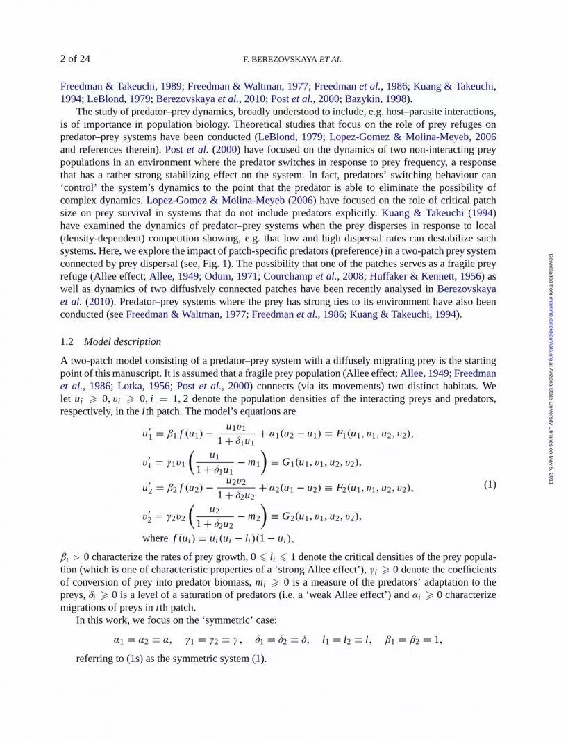
FIG. 1. Schematic for predator–prey interactions: preysui are allowed to migrate between patches, whereas the predatorsvi arenot allowed to migrate. Here,αi , γi > 0, i = 1,2: equation (1) hasαi , γi > 0; equation (2) hasαi = 0, γi > 0; equation (3) hasαi > 0, γi = 0; equation (4a) hasαi > 0, γ2 = 0, γ1 > 0 and (4b) hasαi > 0, γ1 = 0, γ2 > 0.

1.3 Overview of subsystems

The mathematical analysis of Model (1s) advances through an approach that builds on the analyses oflower-dimensional submodels, see Fig.1. For example, we first consider the case when prey dispersal isimpossible. Thus, we have a pair of uncoupled predator–prey (2D) systems. In each patch (α = 0), themodel describes the dynamics of the densities of prey (u) and predator (v):

u′ ≡du

dt= f (u) −

uv

1 + δu,

v′ ≡dv

dt= γ v

(u

1 + δu− m

),

(2)

where f (u) = u(u − l )(1 − u) and parametersl , m, γ, δ are defined as above.System (2) modifies and enhances the classical Volterra model. It has been proposed and inves-

tigated for δ = 0 in prior works (seeBazykin & Berezovskaya, 1979; Bazykin, 1998; Brauer &Soudack,1979;van Voornet al.,2007, etc). Generalizations of this model are studied in recent works(Gonzalez-Olivareset al., 2008;Hilker et al., 2009;Thiemeet al., 2009). It has been shown that the local(one-patch) Model (2) with δ = 0 demonstrates the possibility of prey–predator coexistence in stableequilibrium or in oscillations if parameters are in the appropriate parameter domains (see Fig.2). Weshow below that similar behaviours hold withδ 6= 0. New dynamical modes of population coexistencearise due to prey dispersal between patches in the frame of the bilocal (two-patch) Model (1), whichessentially generalizes the possibility of population persistence.

Thus, System (1s) can be considered as a ‘two-dimensionα-generalization’ of Model (2); it sets thestage for the study of the predator–prey dynamics via the invasion of patch-specific predators.

Note now that System (1s) can be considered also as a ‘two-dimensionγ -generalization’ of themodel (seeFreedman & Waltman,1977;Freedmanet al.,1986):

u′1 = f (u1) + α(u2 − u1) = F1(u1, 0,u2, 0),

u′2 = f (u2) + α(u1 − u2) = F2(u1, 0,u2, 0),

(3)

which describes the dynamics of two Allee-type prey populations interacting diffusely. From this pointof view, System (1s) determines the role of predators in a population community. More exactly, it modelshow the behaviour of the community Model (3) should change with the introduction of their predators.As we will show later, dispersal in a predator-free two-patch environment where the prey must reacha critical mass to survive can support up to nine equilibria including five boundary (one or two prey

at Arizona S


ay 5, 2011im

amm


ownloaded from



populationsare absent) and four co-internal positive equilibria (both prey populations are present) whenthe rate of dispersal is low.

The next subsystem that we consider is the situation when one patch faces predation, while the otheris a refuge (no access to predators). Model (1) can be thought up as a ‘one-dimension generalization’ ofthe two-patch models (Berezovskayaet al., 2010)

u′1 = f (u1) + α(u2 − u1) = F1(u1, 0,u2, v2),

u′2 = f (u2) −

u2v2

1 + δu2+ α(u1 − u2) = F2(u1, 0,u2, v2),

v′2 = γ v2

(u2

1 + δu2− m

)= G2(u1, 0,u2, v2)

(4a)

and

u′1 = f (u1) −

u1v1

1 + δu1+ α(u2 − u1) = F1(u1, v1, u2, 0),

v′1 = γ v1

(u1

1 + δu1− m

)= G1(u1, v1, u2, 0),

u′2 = f (u2) + α(u1 − u2) = F2(u1, v1, u2, 0).

(4b)

Eachof these models describes the dynamics of communities consisting of prey and predator when theprey can disperse between both patches. Systems (4a) and (4b) differ only by designation of variables;we thus omit indices and refer to it as System (4). As we will show in later sections, when predatorshave access to one patch (there is a predator-free or a prey refuge), the system will support one to threepositive equilibria (both prey populations and the predator surviving). These 3D positive equilibriumpoints correspond to boundary (prey–prey plane) equilibria in the absence of the predator.

We show below that the dynamics of System (1s) includes the dynamics of (2), (3) and (4). Inother words, the 2D ‘prey’–‘prey’ system is naturally embedded in the ‘refuge’–‘prey-predator’ system.Similarly, the refuge–prey-predator system is also naturally embedded in the full predator–prey–‘prey-predator’ system. Additionally, however, System (1s) produces its ‘own’ non-trivial 4D behaviours,including the equilibriumAA(u0, v0, u0, v0), u0 = m

1−mδ , v0 = (1−m−mδ)(m−l+lmδ)

(1−mδ)3 andoscillations.These behaviours are the main attention in this work. We will distinguish between ‘trivial’ and ‘non-trivial’ equilibria, the former having at least one zero coordinate. A trivial equilibrium of Systems (1s)and (4) can arise from non-trivial equilibria of System (2) or System (3) and inherit some properties ofthe lower-dimension equilibria. In an effort to understand the complete dynamics of the model commu-nity close to the non-trivial pointAA, we will analyse all equilibria of the model and other non-trivialmodes.

Some of the equilibria have their coordinates given exactly, while others have an asymptotic expan-sion (explicitly to O(a) or O(a2), see Table1). We show that for 0< l < m 6 1, the system can haveup to 16 equilibria from which we distinguish ‘strictly symmetric’ equilibria:u1 = u2, v1 = v2, ‘3D’equilibria possessing one zero coordinate:v1 = 0 or v2 = 0 and ‘2D’ equilibria possessing two zerocoordinates:v1 = v2 = 0.

The paper is organized as follows. In Sections2 and3, we analyse the positions and stability ofthe equilibrium points of model Systems (1s) and its subsystems. We consider also the problem ofthe change of stability with increasing dimension of the subsystems. The results of this analysis inasymptotic form (ona) are summarized in Tables 1 and 2. In Section4, we describe the global dynam-ics of the subsystems in phase-parameter spaces. Section5 contains the results of the analytical and

at Arizona S


ay 5, 2011im

amm


ownloaded from



TABLE 1 Asymptoticcoordinates and eigenvalues (both valid asα → 0 and given explicitly to O(α))associated with the 2D trivial equilibria C of model (1s) forδ = 0

Equilibrium λ1 λ2 λ3 λ4

C0l

(α, 0, l +

α

1 − l, 0

)−γ (m − α) −γ

(m −

α

1 − l

)−l + (1 + 2l ) α l (1 − l ) +

(1 − 3l ) α

1 − l

C01

(α

l, 0,1 −

α

1 − l, 0

)−γ

(m −

α

l

)γ

(1 − m +

α

1 − l

)−l +

(2 + l ) α

l− (1 − l ) +

(3 − l ) α

1 − l

Cl0

(l +

α

1 − l, 0,α, 0

)−γ

(m − l −

α

1 − l

)−γ (m − α) l (1 − l ) +

(1 − 3l ) α

1 − l−l + (1 + 2l ) α

Cl1

(l −

α

l, 0,1 − α, 0

)−γ

(m − 1 +

α

1 − l

)γ (1 − m + α) l (1 − l ) −

(2 − 3l ) α

l− (1 − l ) + (3 − 2l ) α

C10

(1 −

α

1 − l, 0,

α

l, 0

)γ

(1 − m +

α

1 − l

)−γ

(m −

α

l

)−l +

(2 + l ) α

l− (1 − l ) +

(3 − l ) α

1 − l

C1l

(1 − α, 0, l −

α

l, 0)

γ (1 − m + α) −γ(m − l +

α

l

)1 − l −

(2 − 3l ) α

l− (1 − l ) + (3 − 2l ) α

computeranalysis of the 4D behaviours of the Model (1s) that are presented in the form of phase-parameter portraits. Discussion of the outcomes and their biological interpretations are given inSection6.

2. Dynamics of 2D models and equilibria of 3D, 4D models

2.1 Dynamics of System (2)

For α = 0 as well as foru1 = u2, the Model (1s) describes two independent subsystems in the form(2). System (2) has ‘trivial’ equilibriaO0(0,0), Ol (l , 0), O1(1,0) andpositive ‘non-trivial’ equilibriumA(u0, v0), whereu0 = m/(1 − δm), v0 = (1 − m − δm)(m − l + δml )/(1 − δm)3 if 0 < l <m/(1 − δm), m < 1/(1 + δ). The model behaviour is described by the following statements.

THEOREM 2.1 For any fixed parametersγ > 0, δ > 0, the parameter domainM{0 6 m < 1/(1 +δ), 06 l < m/(1− δm)} is divided into five regions of qualitatively different phase portraits of System(2) in the first quadrant (schematically presented in Fig.2).

Boundaries between regions correspond to the bifurcations:S1: m = 1/(1 + δ) andSl : m = l/(1 + δl ), the appearance/disappearance of pointA in the first

quadrant by transcritical bifurcations withO1, Ol , respectively;

H1: l = 2m−1+(1+δ)δm2

1−δ(1−δm)2−δ2m2 , the change of stability ofA in the supercritical Andronov–Hopf bifurca-tion (with the appearance/disappearance of a stable limit cycle);

L: m = m(l ), the disappearance/appearance of a stable limit cycle in a heteroclinic connectioncomposed by the separatrices of equilibriaO1 andOl .1

Theproof of Theorem2.1for small enoughδ is similar to the caseδ = 0 (seeBazykin & Berezovskaya,1979;van Voornet al., 2007).

1Curvem(l ) was found numerically inBazykin & Berezovskaya(1979); it was recalculated with help of the specific computeralgorithm invan Voornet al. (2007).

at Arizona S


ay 5, 2011im

amm


ownloaded from


6 of 24 F. BEREZOVSKAYAET AL.

FIG. 2. Schematically presented parameter-phase portrait of Model (2) for 0 6 m < 1/(1 + δ), 0 6 l < m/(1 − δm). Here,boundaries between domains correspond to the bifurcations:S1 and Sl , the appearance/disappearance of pointA in the firstquadrant by transcritical bifurcations withO1, Ol , respectively,H1, appearance/disappearance of a stable limit cycle in thesupercritical Andronov–Hopf bifurcation,L, the disappearance/appearance of a stable limit cycle in the heteroclinics.

Sketch of the proof.(1) Verifying eigenvalues of trivial equilibria:

λ1(O) = −l , λ2(O) = −γ m; λ1(Ol ) = l (1 − l ), λ2(Ol ) = γ (l/(1 + δl ) − m);

λ1(O1) = −(1 − l ), λ2(O1) = γ (1/(1 + δ) − m),

we prove that the structures of these points are presented in Fig.2. (2) For parameters belonging to theboundaryH1 the first Lyapunov quantityL1, which has been calculated using Bautin’s formula (Bautin,1948), is negative:

L1 = ϕ(γ, l , m)(−4 + δ(4 − 7m) − δ2(4 − 7m+ 7m2) + δ3(8 − 11m)m − 4δ4m2, ϕ(γ, l , m) > 0.

Thus, crossing boundaryH1, we observe that a stable limit cycle is appearing. This cycle is uniquein the model as it follows from criteria (Xiao & Zhang, 2003). As we change parameters, the cycledisappears in the heteroclinic connections of saddlesO1Ol (the latter statement has been verified bycomputations).

2.2 Dynamics of System(3)

For anyα, System (3) has trivial equilibriumO00(0,0) and symmetric non-trivial equilibriaOll (l , l ),O11(1,1). It can also have up to three pairs of ‘non-trivial’ equilibriaC1(u∗

1, u∗2) andC2(u∗

2, u∗1), where

u∗1, u∗

2 are different than the 0, l , 1 roots of the system

F1(u1, 0,u2, 0) ≡ f (u1) + α(u2 − u1) = 0,

F2(u1, 0,u2, 0) ≡ f (u2) + α(u1 − u2) = 0.(5)

at Arizona S


ay 5, 2011im

amm


ownloaded from



To specify relative position of the equilibria, we find equations of the coalescing of equilibrium pointsCin phase-parameter space. The condition is defined by System (5) with the additional requirement that

∣∣∣∣∂(F1(u1, 0,u2, 0), F2(u1, 0,u2, 0))

∂(u1, u2)

∣∣∣∣ ≡ fu(u1) fu(u2) − α( fu(u1) + fu(u2)) = 0. (6)

In the parameter space of Model (3), Systems (5) and (6) define, by the implicit form, the boundarySC,which divides domains where the model has no non-symmetric non-trivial equilibria, has one pair andthree pairs of those (see Fig.3). Analysis of the equilibria as well as the boundaries (5) and (6) werecarried out by expanding the functionsF1(u1, 0,u2, 0), F2(u1, 0,u2, 0) in series inα and consideringthe asymptotic expansion explicitly to O(α). Note that equilibriaC(u∗

1, u∗2) can be considered as those

arising from two of the equilibriaO0, Ol , O1 of System (2) affected by the parameterα. Due to thisfact, we denote theC-equilibria as:C0l , Cl0, C01, C10, Cl1, C1l supposing thatC00 ≡ O00, Cll ≡ Oll ,C11 ≡ O11.

The result of the analysis is collected in the following theorem.

THEOREM 2.2 Positive quadrant(α, l ) consists of three regions of qualitatively different phase por-traits of System (3) (see Fig.3a,c). The curveSC that bounds these regions has two branches whose

FIG. 3. Parameter (a) and corresponding phase (c) portraits of non-symmetric equilibriaC(u∗1, u∗

2) for model (3), non-symmetrictrivial equilibria C(u∗

1, 0,u∗2) for system (4a),C(u∗

1, u∗2, 0) for system (4b) andC(u∗

1, 0,u∗2, 0) for system (1s) correspondingly,

whereu∗1, u∗

2 are roots of (5). There are three pairs of these equilibria in Domain 1, one pair in Domain 2 and no equilibria inDomain 3. (b) Explains the notation ofC-equilibria, C0l , Cl0, C01, C10, Cl1, C1l , as those arising from two of the equilibriaO0, Ol , O1 of system (2) affected by parameterα. C00 ≡ O00, Cll ≡ Oll , C11 ≡ O11 are also presented in the pictures; theyexist for anyα.

at Arizona S


ay 5, 2011im

amm


ownloaded from



asymptoticforms (onα) are

SC1: α1(l ) = 1 − l + l 2 −[(2l − 1)(l − 2)(l + 1)]2/3

2, SC2: α2(l ) =

l − l 2

2.

Threepair of non-trivial equilibriaC01, C10, C0l , Cl0, Cl1, C1l arein the Region 1 bounded by curvesα = 0 andα = α1(l ); one pair of equilibriaC0l , Cl0 is in the Region 2 bounded by curves:α = α1(l )andα = α2(l ) andno equilibria ifα > α2(l ).

For any parameters, the system has two stable nodes:O00(0,0) andO11(1,1) andan unstable nodeOll (l , l ); other equilibria are saddles if they exist.

2.3 Coordinates of 3D and 4D equilibria

Systems (4a) and (4b)

(1) have trivial equilibriaC1(u∗1, u∗

2, 0) andC2(u∗2, 0,u∗

1), whereu∗1, u∗

2 areroots of the System (5).The description of these equilibria was done in Theorem2.2;

(2) have from one up to three pairs of non-trivial equilibriaB1(y, u0, z) and B2(u0, z, y), corre-spondingly, whereu0 = m/(1 − δm)andy, z satisfy

f (y) + α(u0 − y) = 0,

z = ( f (u0) + α(y − u0))/m.(7)

The condition of the coalescing of pairs of equilibrium pointsB is defined by System (7) with theadditional requirement that

fy(y) − α = 0. (8)

In parameter space of Models (4), Systems (7) and (9) defines, by the implicit form, the boundarySBdividing the regions where each system has one equilibriumB and three equilibriaB0, Bl , B1 (seeFig. 4). Removingy from Systems (7) and (9), we have the equation ofSB:

[27αm/(1 − δm) − 9(α + 1)(1 + l ) + 2(1 + l )3]2 + 4(3α − 1 + l − l 2)3 = 0,

α < (1 − l + l 2)/3.

PROPOSITION2.1 The fold bifurcation happens in the Systems (4) for all parameters belonging to thesurfaceSBexcept on the lineα = (1 − l + l 2)/3,m/(1 − δm) = (1 + l )3/(27α); this line correspondsto the cusp bifurcation.

For fixed value of parameterδ, boundarySB consists of two branchesSB12, SB23:

SB12: m/(1 − δm) =9(α + 1)(1 + l ) + 2(1 − l + l 2 − 3α)3/2

27α,

SB23: m/(1 − δm) =9(α + 1)(1 + l ) − 2(1 − l + l 2 − 3α)3/2

27α.

Equilibria B0, Bl coalesceat the boundarySB12 andequilibria Bl , B1 coalesceat the boundarySB23(seeFig. 4, given for caseδ = 0); at the cusp parameters equilibriumB has the coordinatesy =(1 + l )/3,z = 0.

at Arizona S


ay 5, 2011im

amm


ownloaded from



FIG. 4. Parameter (a) and corresponding phase (b) portraits of non-trivial equilibriaB2(u0, z, y) for Model (4b), B1(y, u0, z)for Model (4a), trivial equilibriaB2(u0, z, y, 0) andB1(y, 0,u0, z) for System (1s) correspondingly, wherey, z are roots of (7).System (1s) has three pairs of these equilibria in Domain 2 (B0

1, Bl1, B1

1, B02, Bl

2, B12) and one pair in Domain 1 (B1, B2). The

boundary between domains corresponds to the fold bifurcation in any points except the upper point corresponding to the cuspbifurcation.

As in the previous case, analysis of coordinates of the ‘non-boundary’ equilibriaB has been doneby expanding the functionsF1(u1, 0,u2, v2), F2(u1, v1, u2, 0) in a series for smallα and consideringthe asymptotics explicitly to O(α) or O(α2): By(a)(y, u0, z) = limα→0 B(y(α), u0, z(α)).

For example,y(B1) = 1 − (1−m(1+δm))α(1−l )

( (1−(2−l )m(1+δm))(1−l )2 − α

)

Now, we are ready to describe coordinates of equilibria of the 4D System (1s).

THEOREM 2.3 For arbitrary positiveα, System (1s)

• has up to three pairs of trivial ‘2D’ equilibriaC1(u∗1, 0,u∗

2, 0) andC2(u∗2, 0,u∗

1, 0), whereu∗1, u∗

2 aredistinguished from the 0, l , 1 roots of the System (5); the relative position of these equilibria is givenin Theorem2.2(see also Fig.3);

• has from one up to three pairs of trivial 3D equilibriaB1(y, 0,u0, z) andB2(u0, z, y, 0), wherey, zsatisfy (7) andu0 = m/(1 − δm); the relative position of these equilibria is given in Proposition2.1(see also Fig.4);

• has trivial symmetric equilibriaO(0,0,0,0), Oll (l , 0, l , 0), O11(1,0,1,0) and if 06 m < 1/(1 +δ), 06 l < m/(1−δm) has also non-trivial oneAA(u0, v0, u0, v0), whereu0 = m/(1−δm), v0 =(1 − m − δm)(m − l + δml)/(1 − δm)3 (see Theorem2.1and Fig.2).

3. Stability of equilibria

3.1 On lower-dimension non-trivial equilibrium and higher-dimension trivial equilibrium

Each of the equilibria of Systems (2) and (3) has its ‘image’ in the frame of Models (4), (1s) or both.Note that such ‘imaging’ equilibrium can be trivial, whereas the equilibrium of lower dimension were

at Arizona S


ay 5, 2011im

amm


ownloaded from


10of 24 F. BEREZOVSKAYA ET AL.

non-trivial ones. We show below that the imaging equilibrium can be unstable, whereas the ‘pre-image’was stable.

We first consider the equilibria denoted asC, which are non-trivial in the 2D System (3) and becometrivial in both the 3D Systems (4) and the 4D System (1s). The Jacobians of System (3) at equilibriumC(u1∗, u2∗), System (4a) atC(u1∗, 0,u2∗) andSystem (1s) atC(u1∗, 0,u2∗, 0) are,respectively:

J2 =

(P1(C) α

α P2(C)

)

, J3 =

P1(C) α 0

α P2(C)−u∗

21+δu∗

2

0 0 S2(C)

, J4 =

P1(C)−u∗

11+δu∗

1α 0

0 S1(C) 0 0

α 0 P2(C)−u∗

21+δu∗

2

0 0 0 S2(C)

,

whereP1(C) = fu(u∗1) − α, P2(C) = fu(u∗

2) − α; S1(C) = γ (m −u∗

11+δu∗

1), S2(C) = γ

(m −

u∗2

1+δu∗2

)

and f (u) = u(u − l )(1 − u). These Jacobians have characteristic polynomials, which are equal,respectively, to

φ2(λ) = (P1(C)−λ)(P2(C)−λ)−α2, φ3(λ) ≡ φ2(λ)(S2(C)−λ), φ4(λ) ≡ φ3(λ)(S1(C)−λ). (9)

So,each successive characteristic polynomial differs from the previous one only by one factor.Similar arguments hold for the 3D and 4D pointsB. The Jacobians of Systems (4) atB1(y, u0, z)

and(1s) atB1(y, 0,u0, z) are,respectively,

J3 =

P1(B) α 0

α P2(B) −m

0 γ z(1 − δm)2 0

, J4 =

P1(B) −y1+δy α 0

0 S1(B) 0 0

α 0 P2(B) −m

0 0 γ z(1 − δm)2 0

,

whereP1(B) = fu(y) − α, P2(B) = fu(u0) − α − z(1 − δm)2; S1(B) = γ(m − y

1+δy

).

TheseJacobians have characteristic polynomials, which are equal to

ϕ3(λ) = −λ(P1(B)−λ)(P2(B)−λ)+γ mz(1−δm)2(P1(B)−λ)+α2λ, ϕ4(λ) = ϕ3(λ)(S1(B)−λ)(10)

andso differ by only one factor. Thus, the following statement holds.

PROPOSITION 3.1 (1) Let u1, u2 be roots of System (5). Then, Systems (3), (4) and (1s) have twoidentical eigenvaluesλ1, λ2 at equilibriaC(u1, u2), C(u1, 0,u2) andC(u1, 0,u2, 0); Systems (4) and(1s) have three identical eigenvaluesλ1, λ2, λ3 atequilibriaC(u1, 0,u2) andC(u1, 0,u2, 0);

(2) Let u1, v2 be roots of System (7). Then, Systems (4a) and (1s) have three identical eigenval-uesμ1, μ2, μ3 at equilibria B(u1, u0, v2) and B(u1, 0,u0, v2), correspondingly. The same is true foreigenvalues of equilibriaB of Systems (4b) and (1s).

Models (4) have up to 12 equilibria: up to nine trivial equilibriaC andO (see Fig.3 and Theorem2.2) and up to three non-trivialB (see Fig.4 and Proposition2.1); Model (1s) including two ‘submodels’(4a), (4b) has up to 16 equilibria: 12 trivial,C and O, 3 trivialB and 1 non-trivialAA (see Theorem2.3).We use Proposition 2.2, series expansions inα, as well as computer experiments in the analysis of theirstability.

at Arizona S


ay 5, 2011im

amm


ownloaded from


A BIFURCATION APPROACH 11of 24

3.2 Non-trivial equilibria B of Model (4)

For α > 0, System (4a) has from one up to three non-trivial equilibriaB(u1 = y, u2 = u0, v2 =z), where y, z satisfy (7) (see Proposition2.1 and Fig.4). Inside the region bounded by the curveSB12 ∪ SB23 (seeFig. 4a), System (4a) has three equilibriaB0, Bl , B1 (Domain2 in Fig.4a,b), whileoutside of this region, there exists only oneB (Domain 1 in Fig.4a,b). The coalescing ofB0, Bl happenswith parameter values at the branchSB12 andthe coalescing ofBl , B1 happensat the branchSB23.We consider the former case (because it happens with reasonable parameter valuesα, m, l ≈ 0.1 −0.3 for fixed γ ≈ 1, seeBerezovskayaet al. (2010) for details). Note that the coalescingB0, Bl atSB12 doesnot change the qualitative properties ofB1, which becomesB along the upper parameterbranchSB12.

Thestability characteristics of the equilibriumB(u1, u0, v2) is determined by the roots of the char-acteristic polynomialϕ3(λ) (see(10) and Table2) at the valuesu1 = y, v2 = z. Analyzing (7) and (10)and accounting (8), we get the following proposition.

PROPOSITION3.2 (i) If equilibrium B(u1, u0, v2) is a simple one, then the associated eigenvalues aregiven, accurately to O(α), by the formulas:λ1 = f ′(u1) − α, i.e. λ1 = λ1(B0) = −l + O(α), orλ1 = λ1(Bl ) = l (1 − l ) + O(α), or λ1 = λ1(B1) = l − 1 + O(α) andλ2,3 satisfy the equationλ2 − ( f ′(m/(1 − δm)) − α − v2((1 − δm)2)λ + γ mv2(1 − δm)2 = 0.

TABLE 2 Asymptotic(as α → 0) coordinates up to O(α2) and eigenvalues up to O(α) associatedto the 3D trivial equilibria B1(m, y, x, 0), B2(x, 0,m, y) of Model (1s) for parameter valuesδ = 0and27αm − 9(α + l )(1 + l ) + 2(1 + l )3 + 4(3α − 1 + l − l 2)3 < 0

B10(m, y, x, 0) B1

l (m, y, x, 0) B11(m, y, x, 0)

x = mα

l+ m (m − l + ml )

α2

l3, x = l − (m − l )

α

l (1 − l ), x = 1 − (1 − m)

α

l (1 − l )−

y = (m − l ) (1 − m) − α(1 −

α

l

)y = (m − l ) (1 − m) −

(m − l )

mα (1 − m) (1 − 2m+ lm)

α2

(1 − l )3,

y = (m − l ) (1 − m) −(1 − m) α

m

λ1 −γ m(1 −

α

l

)−γ (m − l )

(1 −

α

l (1 − l )

)γ

1 − m

1 − l

(1 −

(1 + lm − 2m) α

(1 − l )2

)

λ2 −l + (2ml + 2m− l )α

ll (1 − l ) −

2(1 − 2l ) (m − l ) α

l (1 − l )− (1 − l ) +

(3 − l − 4m+ 2lm) α

(1 − l )

λ3,4Tr1 ±

√δ1

2, where

Tr2 ±√

δ2

2, where

Tr3 ±√

δ3

2, where

Tr1 = (1 + l − 2m) m− Tr2 = (1 + l − 2m) m− Tr3 = (1 + l − 2m) m−

(1 − m) α (1 + l − m) α (2 − m) α

δ1 = Tr 21− δ2 = Tr 2

2− δ3 = Tr 23−

4γm (m − l ) (1 − m) + 4γm (m − l ) (1 − m) + 4γm (m − l ) (1 − m) −

4γmα 4γ (m − l ) α 4γ (1 − m) α

at Arizona S


ay 5, 2011im

amm


ownloaded from



(ii) Equilibrium B1/B changesstability in the Hopf bifurcation with parameter values belonging tothe surface, which forms (correctly to (o(α2)) :

H δ3 ≡ H δ(B1/B) = H0(B1/B) − H1(B1/B)mδ + H2(B1/B)(mδ)2 − H3(B1/B)(mδ)3 = 0,

whereH0(B1/B) = (1 − m)α2 − (1 − l )α + m2(1 − l )(1 + l − 2m),

H1(B1/B) = (m(l + m2)(1 − l ) + α(m − 4)(1 − l ) + α2(4 − 3m),

H2(B1/B) = m(1 − l )(l (m − 2) + m)) + 2α(1 − l )(m − 3) − 2α2(m − 3),

H3(B1/B) = ml (1 − l ) + α(1 − l )(m − 4) + 2α2(m + 2).

REMARK For δ = 0, we denoteH3 ≡ H0(B1/B), the Hopf bifurcation surface.

3.3 Symmetric equilibria of Model (1s)

For the arbitrary equilibrium, Jacobian matrix∂(F1,G1,F2,G2)∂(u1,v1,u2,v2)

of System (1s) a specific block-diagonal

form (similar toJ4, J4 above) is present, which significantly simplifies calculations of its eigenvalues.

PROPOSITION3.3 The eigenvalues of the System (1s) with 06 m < 1/(1 + δ), 0 6 l < m/(1 − δm)at the symmetric equilibriaO(0,0,0,0), Oll (l , 0, l , 0), O11(1,0,1,0) and AA(u0, v0, u0, v0), whereu0 = m/(1 − δm), v0 = (1 − m − δm)(m − l + δml )/(1 − δm)3 are,respectively,

λ1(O) = λ2(O) = −γ m, λ3(O) = −l , λ4(O) = −l − 2α;

λ1(Oll ) = λ2(Oll ) = −γ (m − l/(1 + δl ), λ3(Oll ) = l (1 − l ), λ4(Oll ) = l (1 − l ) − 2α;

λ1(O11) = λ2(O11) = γ (1/(1 + δ) − m), λ3(O11) = −(1 − l ), λ4(O11) = −(1 − l ) − 2α;

λ1,2(AA) =P − α ±

√((P − α)2 − 4mγ Q)

2, λ3,4(AA) =

P + α ±√

((P + α)2 − 4mγ Q)

2where

P = −α + (1 − m/(1 − δm))(1 − m − δlm) + fu(m/(1 − δm)),Q = −(1 − m/(1 − δm))(1 − m − δlm).

We omit the proof of the Proposition, referring the reader.

REMARK For δ = 0, the eigenvalues of equilibriumAA are given by

λ1,2(AA) =mn±

√((mn)2 − 4mγ v∗)

2, λ3,4(AA) =

mn− 2α ±√

((mn − 2α)2 − 4mγ v∗)

2,

wheren = 1 + l − 2α.

Furtherinvestigation of the basic Models (1s) and (4) is based mainly on computer experiments sup-plemented by analytical hypotheses. Although we consider the caseδ = 0 to simplify calculations, themain results do not change (at least) for smallδ.

4. Dynamics of Models (4a)

4.1 (m, α)-bifurcation diagram of System (4a)

Let us consider dynamics of the 3D System (4) taken in form (4a), prey–prey-predator. The detailedanalysis of the model has been provided inBerezovskaya(2006) andBerezovskayaet al. (2010), based

at Arizona S


ay 5, 2011im

amm


ownloaded from



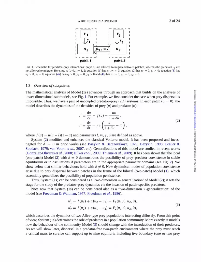
FIG. 5. The schematic parameter portrait of System (4a) is given forγ = 1 andl = 0.1. In this portrait, surfaces that correspond tothe bifurcations of co-dimension 1 are presented as lines (the boundaries of different domains). Lines corresponding to bifurcationsof co-dimension 2, ‘1 + 1’ or higher are presented as points on these lines. The meaning of each bifurcation boundary is describedin “Theorem4.1”. Sequences of phase portraits are done in Figs7 and8.

FIG. 6. Heteroclinic connection between two trivial equilibrium points.

on results of Theorem2.2, Propositions2.1,3.2,4.1and computations with help of specialized packagesTRAX (Levitin, 1989) and LOCBIF (Khibnik et al., 1993). Here, we describe some main properties ofthe model behaviour which are collected in the following statements (see Figs5–8)

“THEOREM 4.1” 2Let γ = 1 andδ = 0. For positive values of the variablesu1, u2, v2, small enoughvalues of the dispersal parameterα, and l < m, the parameter portrait of System (4a) is dividinginto 7 domains supporting qualitatively different stable phase behaviours; boundaries of these domainscorrespond to the following bifurcations in the model. Boundaries of co-dimension 1 of local bifurca-tions, including saddle-node (fold)SB12 ∪ SB23 for non-trivial equilibriaB0, Bl , B1 and Hopf bifur-cationsH3(B) of positive non-trivial equilibriumB1/B have been found (existence). The parameterportrait of System (4a) also contains boundaries corresponding to the non-local bifurcations, namely,multiple-limit cycle bifurcation C, heteroclinic bifurcationPc from the separatrices of trivial

2Quotations mean that the results have been obtained by computations and not only strictly analytically. Further theorems omitquotations but are understood similarly.

at Arizona S


ay 5, 2011im

amm


ownloaded from



FIG. 7. A sequence of phase portraits, Domains 1, 2, 3, 6, 7, asαvaries forδ = 0, γ = 1, m = 0.4, l = 0.1. Domain 1 (α= 0) toDomain 2 (α = 0.01, 0.05) to Domain 3 (α = 0.1,0.18,0.8) to Domain 6 (α = 0.9) to Domain 7 (α = 2). Specifically, the stabledynamics shift from extinction (equilibrium(0,0,0)) to a bi-stable situation (a stable oscillations plus equilibrium(0,0,0)) andagain to extinction.

non-symmetric equilibrium points and a heteroclinic bifurcationP0 consisting of the separatrices ofthe trivial symmetric equilibrium pointsCll andC11.

The schematic parameter portrait of System (4a) forγ = 1 is given in Fig.5 as the(m, α)-slice ofcomplete(m, α, l )-space forl = 0.1. Sequences of phase portraits in different parameter domains arepresented in Figs7 and8.

4.2 Boundaries of the domains: equilibria and limit cycles

Together with equilibria, which have been studied in Theorem2.2 and Propositions2.1, 3.2, System(4) also supports limit cycles. We first consider those cycles that arose with the change of stability ofthe equilibriumB1/B at the boundaryH3. The direction of the bifurcation is determined by the sign ofthe first Lyapunov quantityL1 on H3; the bifurcation is ‘supercritical’ ifL1(H3) < 0 and ‘subcritical’if L1(H3) > 0 (Andronovet al., 1971;Guckenheimer & Holmes, 1996;Guckenheimer & Kuznetsov,2007;Kuznetsov, 1995).

For l = 0.1, curveH3 consists of two positive branches,H3 = H13 ∪ H2

3 (see Fig.5). The followingstatement describes the Hopf bifurcation ofB1/B.

PROPOSITION4.1 Letm > l . The equilibrium pointB1(or B) changes stability via a supercritical Hopfbifurcation onH1

3 ≡ H1+3 . Consider curveH2

3 = H2+3 ∪ H2−

3 . The equilibriumB changes stability ina supercritical fashion when parameters belong to the interior ofH2+

3 and in a subcritical fashion whenparameters belong to the interior ofH2−

3 ; L1(H2+3 ∩ H2−

3 ) = 0.

at Arizona S


ay 5, 2011im

amm


ownloaded from



FIG. 8. (a) Transitioning from Domain 3 to Domain 5 as we cross boundaryC where a pair of limit cycles (stable and unstable)appear. A sequence of phase portraits is presented for smallσ = m − l . Here, the parametersm = 0.27, l = 0.1 andγ = 1,δ = 0 are fixed andα changes from Domain 3 (α= 0.35) to Domain 5 (α = 0.468), to Domain 6 (α = 0.48) and to Domain7 (α = 0.5) as the dynamics change. Specifically, the change is from the stable equilibrium(0,0,0) to a stable limit cycle, tothe stable non-trivial equilibrium, to a tri-stability situation, to the bi-stability and, finally, to extinction (the only stable mode isequilibrium(0,0,0)). (b) γ = 1, m = 0.37, l = 0.3. The phase portrait from Domain 4 is given forα = 0.31 and in Domain 3for α = 0.2.

REMARK As parameterl increases, curveH3(l ) changes its shape and for certainl = l (α, m, γ ) ‘loses’the ‘point’, whereL1(H3) = 0. Then, for any fixedl < m < 1, it takes the shape of theH≡

3 H1+3 and

point B1 (or B) changes stability via the supercritical Hopf bifurcation only.

Generalized Hopf bifurcation (of co-dimension 2), also called the Bautin bifurcation (Guckenheimer& Kuznetsov, 2007;Kuznetsov, 1995), is realized for parameter values, whereL1(H2+

3 ∩ H2−3 ) = 0. It

is known that a ‘saddle-node bifurcation’ of cycles (co-dimension 1) has to be observed closely.

PROPOSITION4.2 The parameter space of System (4) contains the boundary surfaceC of multiple-limitcycles, which corresponds to a non-local bifurcation of the collision and annihilation of two cycles. Theparameter values inH3 whereL1(H3) = 0 also belong toC (see Fig.5).

at Arizona S


ay 5, 2011im

amm


ownloaded from



Thenon-local ‘heteroclinic bifurcations’ also occur in System (4). Trivial equilibriaC andO playa key role in the appearance of heteroclinic limit cycles as shown in Fig.6. In fact, there exist two typesof heteroclinics, which are realized with parameters at boundariesPc andP0 in the parameter portrait ofthe system given in Fig.5. The boundaryPc has0 < α < α1(l ) (see,SC1 in Fig. 3) and the respectiveheteroclinics connect non-symmetric equilibria in the phase space. The boundaryP0 hasα > α2(l ) (see,SC2 in Fig.3) and the respective heteroclinics connect the trivial symmetric equilibriaCll andC11. Notethat the heteroclinic bifurcation results in the appearance/disappearance of a limit cycle in phase space.We have verified by computations that forγ = 1, l = 0.1, the limit cycle is stable forPc andcan bestable as well as unstable forP0. We denoteP0 asP+

0 , P−0 in the former and latter cases (similar to the

previously discussed Hopf bifurcations where the signs ‘+’ or ‘−’ denote the stable or unstable limitcycle that appeared in the phase space as a result of the change in the stability of equilibriumB).

4.3 Dynamics interpretations

We now fix the non-dispersal parameters in Domain 4 (see Fig.2) of System (2); i.e. we start with thenon-dispersal parameters that lead to the extinction of the prey and predator populations as we explorethe role of dispersal. We do not discuss the model community behaviour in Domain 1 where dispersalα is very small, instead stating that only equilibrium points(0,0,0) and(1,1,0) are stable there forSystem (4a).

As α increases (moving into Domain 2), oscillations are observed from the occurrence of a het-eroclinic bifurcation. The amplitude of the oscillations decreases asα increases. Afterα crosses theboundary of the Hopf bifurcationH1+

3 (moving into Domain 3), the oscillations stop and a stable equi-librium becomes the attractor (see, Fig.7). Behaviour of the system asα increases further depends onthe differenceσ = m − l . For largeσ , increases inα lead to stable oscillations (Domain 6), whicharise from the crossing of the boundaryH2+

3 with a second supercritical Hopf bifurcation. Crossing theheteroclinic boundaryP+

0 , one comes to Domain 7 where(0,0,0) is the unique attractor. Thus, largevalues ofα (in Domain 7) lead all populations (surprisingly) to extinction. For smallσ asα increases,we observe changing dynamics as we move through Domains 3→ 4 → 7. Parameter values on theboundaryP−

0 correspondto the appearance of an unstable limit cycle in Domain 4. This cycle, asα

increases, shrinks to the equilibriumB on H2−3 . Subsequently, the equilibriumB loses its stability and

the origin remains as the only attractor (in Domain 7). The difference of behaviours in Domains 3 and4 can be seen from Fig.8b. For intermediate values ofσ , we observe tri-stability in Domain 5. In fact,(0,0,0), stable non-trivial equilibriumB, and a stable limit cycle co-exist. A sequence of dynamicsincluding the tri-stability is shown in Fig.8a forδ = 0, γ = 1, l = 0.1, m = 0.27 asα changes from0.35 to 0.5.

Overall preliminary results of analysis of Model (4) have shown that behaviours of this system, whenparameters vary, are much more complicated and diverse than the behaviour of Systems (3) and (2) fromwhich it was generalized. The model populations can coexist in equilibrium or oscillations, whereas thepopulation system described by Model (2) goes to extinction with the same parameter values.

5. Dynamics of Model (1s)

5.1 Change of stability of non-trvial equilibrium

According to Proposition3.3, System (1s) can have only two strictly stable equilibriua:

O(0,0,0,0), AA(m, v∗, m, v∗), v∗ = (m − l )(1 − m).

at Arizona S


ay 5, 2011im

amm


ownloaded from



The former is stable for all parameters and the latter is stable in some parameter domains and unstablein others. Recall that equilibriumA(m, v∗), the pre-image ofAA in the frame of System (2) forδ = 0,loses stability in the supercritical Andronov–Hopf bifurcation with parameter values belonging to theboundary curveH1: m = (l + 1)/2 (see, Theorem2.1and Fig.2 containing (l , m)-parameter portrait of(2)). According to the Remark following Proposition3.2, this boundary also serves as one of the Hopfbifurcation boundaries in System (1s) because Re(λ1,2(AA)) = 0 for these parameters. We denote this‘old’ boundary asH1{γ, α, m, l : m = (l + 1)/2 }. The second, ‘new’ branch of the Hopf bifurcation,H2{γ, α, m, l : α = m(l + 1 − 2m)/2}, corresponds to the vanishing of the real parts of eigenvaluesλ3,4(AA).

PROPOSITION5.1 Let 0 < l < m. Equilibrium AA(m, v∗, m, v∗) of System (1s) located in the first or-thant of the(u1, v1, u2, v2)-phasespace changes stability in a supercritical Andronov–Hopf bifurcationwith parameter values belonging to the surfaceH1 for anyγ > 0 and to surfaceH2 for any 0< γ 6 1.

Proof. We have calculated the first Lyapunov quantitiesL1 at H1 andH2 (seeBautin,1948,Huffaker& Kennett,1956). Applying the procedure contained inGuckenheimer & Kuznetsov(2007) we obtain

L1(H1) = −c1(l + 1)/(2γv∗),

and

L1(H2) = c2(−8α2(4 + 4l − γ − 6m) − 9(1 + l )γ mv∗ − 2α((8 + 8l 2 + 2γ − γ 2 + 2l (8 + γ ))m−

6(8 + 8l + γ )m2 + 72m3 + 2γmv∗)), α = m(l + 1 − 2m)/2,

wherec1, c2 arepositive.It is evident thatL1(H1) < 0. Numeric analysis ofL1(H2) hasshown thatL1(H2) < 0 for reason-

able values of parameters. This completes the proof. �Our computer experiments with System (1s) revealed that the stable cycle, which appears when

crossing the boundaryH2, disappears with parameter values very close to those inH2, annihilating withan some unstable limit cycle. Because of this, we did not mention the domain of its existence in theparameter portrait of System (1s), see Fig.9, and noteH2 is the dotted line there. The stable cycle,which appears crossing the boundaryH1, exists for a wide parameter domain; we call this cyclecu.

5.2 4D oscillations in System (1s)

Computational analysis of the System (1s) (provided by use of packagesLevitin, 1989;Khibnik et al.,1993) reveals the complicated structure of its dynamics, which essentially depends on parameter valuesof the system as well as on initial values of the variables. Of course, due to biological interpretations ofthe Model (1s), our main interest is in the ‘stable’ modes, which can be observed with variations of initialdata. We show that even for fixed parameters, the system can demonstrate wide range multistability. Inaddition, the existence of migration in our model increases diversity of stable modes thereby increasingthe sustainability of the model community.

The schematic parameter portrait of the system for some typical 4D rearrangements of model be-haviours in a phase neighbourhood of pointAA is presented in Fig.9. The portrait represents an(m, α)-cut of the 4D(α, γ, m, l )-parameter space for fixed valuesγ = 1 and 0< l = 0.1 < m < 1, such that(l , m) belongs to Domain 4 or adjacent to the boundaryL Domain 3 in Fig.2. The portrait was obtainedby analytical and computer methods of bifurcation theory. The analytically obtained curvesH1, H2 ofthe Hopf bifurcations were described above. One more boundary, the curveF, was verified with help

at Arizona S


ay 5, 2011im

amm


ownloaded from



FIG. 9. (a) Schematically presented(α, m)-cut of the(δ = 0, γ = 1, l = 0.1, α,m)-parameter portrait of 4D stable modes ofModel (1s). Domain 1 contains the stable non-trivial 4D equilibrium, Domain 3 has no non-trivial 4D attractors. (b) Phase portraitsin Domains 2, 4 and 5.

by the software TRAX (Levitin, 1989). We believe that the computer Package developed invan Voornet al. (2007) can be useful for recalculations of the separatrix boundariesL1 andF as it was done in thecase of the Model (2).

The 3D rearrangements of the model behaviour (see Figs5, 7, 8) are not presented in this portrait;they was discussed above.

In Domain I of the parameter portrait the model has a stable 4D equilibriumAA. In Domain II,the model has stable oscillations corresponding to the stable 4D limit cycle ‘cu’ in (u1, v1, u2, v2)-phase space. This cycle appears when we cross boundaryH1 as m decreases (from right to left inFig. 9) and equilibriumAA loses stability in the 2D eigenspace, whereas the other 2D eigenspacecorresponds to trajectories tending toAA ast → ∞. The cyclecu exists for anyα > 0 and disappears(asm decreases) at heteroclinics composed by separatrices of the trivial symmetric equilibriaOll , O11

(see Fig.10). The parametric boundary (schematically presented as a straight line corresponding to thementioned heteroclinics) is denotedL1 in the portrait (Fig.9). Cyclecu has pre-image in System (2) thatalso has appeared in a supercritical Andronov–Hopf bifurcation after crossing boundaryH ≡ H1 anddisappeared at heteroclinics ofOl , O1 (see Fig.2). With fixed value ofl = 0.1, linesL1 in Fig. 9 andLin Fig. 2 has a common point forα = 0: m ≈ 0.446.

In Domain III, the model has only one 4D attractor, equilibrium at the origin.Model (1s) demonstrates its most interesting 4D behaviour in Domains IV and V bounded by curve

F at the portrait in Fig.9. Our computer analysis has revealed that for very smallα (close to the boundarySC1 in Fig. 3) and a wide range ofm, the separatrices of the trivial 2D equilibriaC10, C01 give rise tothe 4D limit cyclec4 (see Fig.10b whereα = 0.001 and both cyclesc4 andcu are presented).

For fixed values ofl increasingα results inc4 undergoing period doubling, whereby it loses itsstability transforming to a torus, etc., depending on the value ofm for which we consider this cycle.Figures11a and b, wherem = 0.45, α = 0.0256 andα = 0.0235, respectively, display the stages ofperiod doubling ofc4 in Domain IV. In Fig.11b, one can observes period doubling in more detail; it isclear from this picture that the domains of attraction ofcu andc4 are divided by an unstable manifold

at Arizona S


ay 5, 2011im

amm


ownloaded from



FIG. 10. (a) Limit cyclecuappears in the supercritical Hopf bifurcation withm = 0.55 and disappears in heteroclinics withm ∼= 0.445; (b) In Domain 4 limit cyclesc4 andcu coexist for parametersα = 0.001,m = 0.46,γ = 1, l = 0.1, 3D cyclec0 isalso presented.

FIG. 11. Period doubling of cyclec4 in Domain 4: (a)α = 0.0256,m = 0.45; (b)α = 0.0235,m = 0.48; here, cyclecu is alsopresented.

at Arizona S


ay 5, 2011im

amm


ownloaded from



similar to a limit cycle. Note that limit cyclec4 is destroyed at Domain IV under some period doubling,presumably, Feigenbaum doubling that gives rise to a cycle of period 3 which leads to the appearance ofweak chaotic dynamics (Lopez-Gomez & Molina-Meyeb,2006;Kuznetsov, 1995). Cyclec4 destructs atthe boundaryF (see Fig.9). Aperiodic oscillations are observed in the model at that part of the boundaryF, which divides Domains IV and II.

In Domain V, increasingα results in cyclec4 transforming to a torus (whenm decreases, seeFig. 12). This torus possessing irrational rotating number (see two left pictures in Fig.14, m = 0.345,m = 0.315, withα = 0.027) is destroyed by the appearance of a rational rotation number (see Fig.12,right, m = 0.315 withα = 0.028, this parameter point is in the left side of the boundaryF of DomainsV and III) and chaotic dynamics result (seeGonzalez-Olivareset al., 2008for theory of general torusdestruction). In Fig.13, we show portraits of the system form = 0.42, α = 0.032; this parameter pointis in the upper part of the boundaryF. One can observe there the ‘special torus’ with irrational rotationnumber.

According to our analysis and the given bifurcation diagram let us note that the stable limit cyclec4exists in the Model (1s) with parameter valuesm (Domain V) for which one-patch Model (2) has theonly one attractive equilibrium:O, i.e. community coexist with wider range of parameters.

The portraits, shown in Fig.14, display two stable manifolds: two-leaf torusc4 and 3D cyclec3;initial points in their basins are distinguished only in theiru-coordinate,u = 0.01 for the former and

FIG. 12. Changing cyclec4 with decreasing of parameterm in Domain 5.

FIG. 13. Irrational rotating number atc4 in Domain 5

at Arizona S


ay 5, 2011im

amm


ownloaded from



FIG. 14. Stable ‘cycles’c4 andc3 coexists in Domain 5.

u = 0 for the latter. Remind that stable manifolds (presumably, limit cycles) of 3D model can beobserved in the frame of 4D Model (1s) for suitable in initial data (see Fig.10b where 3D cyclec0 isalso presented), however with rather specific basins.

Our computations revealed that (1s) simultaneously has 4D and 3D attractors, limit cycles, for awide range of parameters. The origin equilibrium is stable for any parameter values, though its basin ofattraction can vary. Thus, the model community can tend to one of these depending on initial values.Thus, the Model (1s) supports multistability for a wide parameter domain.

6. Discussion and interpretations

It is useful to compare dynamics of the three models described by the 2D System (2), 3D System(4) and 4D System (1s). All these models reflect by the simplest form (strong) Allee effect in preypopulations and the saturation (expressed by Holling 1 type trophic functionBazykin, 1998;Brauer& Soudack, 1979;Gonzalez-Olivareset al., 2008etc.) in predator population, sometimes called weakAllee effect; Models (4) and (1s) describe also the possibility for preys to migrate diffusively betweenpatches. The Allee effect is characterized in the models by parameterl > 0, the critical densities ofthe prey populations, parametersα, m > 0 serve, respectively, as measures of prey migrations betweenpatches and the predators’ adaptation to the preys, parameterδ > 0 reflects saturation andγ denotes thecoefficients of conversion of prey into predator biomass. The main attention was given in the work tothe caseγ = 1 in all models and to fixed smallδ. Variations of these parameters can lead, certainly, toappearance of new dynamic effects in the model behaviours but have to keep gotten effects.

The two-parameter(m, l )-model of the local (one-patch) community (2) predicts, depending onparameter values (see Fig.2), four different domains of dynamical behaviour: getting predators toextinction with any initial density because the death rate of predators is too large, possibility of predator–prey coexistence at steady state or stable oscillations for a wide range of initial densities and gettingpreys and predators to extinction because predators over-regulate prey density.

The three-parameter(m, l , α)-model of two-patch community (4) describing dynamics of preys andpredator–preys systems even for fixed value of parameterl = 0.1 supports seven parametrically sta-ble domains of different dynamical behaviours (see Figs5, 7, 8). We note the possibility of populationcoexistence for a wide range of initial densities and parameters. It was shown that for suitable disper-sal prey rates between both patches, the predator can control the numbers of both prey populations ina stable equilibrium or in oscillatory regimes. It was revealed also that trivial 2D equilibrium pointsin the frame of Model (4) ‘originate’ oscillations in the community after their separatrices compose

at Arizona S


ay 5, 2011im

amm


ownloaded from



heteroclinics.(The interpretation tells us that the stability of the community is provided by ‘migrantoffspring’.) The most diverse behaviours of this model are observed close to boundaries of populationcoexistence. Regimes of bi-stability or tri-stability were found: depending on initial data, the modelcommunity can coexist at a non-trivial stable equilibrium, at stable oscillations or go extinct. It is im-portant to note that both subsystems in the model community can survive for parameter values for whichany one of them would go to extinction for all initial densities in isolation.

The three-parameter(m, l , α)-model (1s) describing dynamics of the two-patch predator–prey sys-tems supports more diversity of stable modes in comparing with Model (4) at least because (1s) can beconsidered asγ1/γ2-‘generalization’of (4). However, forγ1 6= 0/γ2 6= 0, System (1s) ‘holds’ the mainstable dynamics of (4) forv1 = 0/v2 = 0. It means that ifv2 = 0, then System (1s) will display alldynamic portraits which we have observed for (4). Note that these portraits can be unstable with respectto ‘invasion’ of predatorsv2.

Thestable 4D modes of Model (1s) are collected with the schematic bifurcation diagram in Fig.9.The parameter portrait of the system is divided into five domains comprising different 4D phase be-haviours of the model. First of all note that the model demonstrates the existence of stable 4D limitcyclecu which is strictly ‘succeeding’ to the limit cycle of 2D System (2). The limit cycle appears whenthe non-trivial equilibrium changes its stability within Hopf bifurcation and disappears on heteroclinics(see Fig.10a). This fact can be interpreted as follows: predators get weaker (m ↓) leads to transformingof a stable mode from equilibrium to oscillations with growing period and getting extinction at last.

Note now that we found numerically one more stable 4D limit cyclec4 in the Model (1s). For anyfixed reasonable values of parameterm, this cycle is observing in the space for very small values ofmigration parameterα (Domain 4 in Fig.9). We suppose that this cycle arises as the special combina-tions of two limit cycles of subsystems (4a) and (4b) (see Fig.6). With growth ofα, for fixed largerm,we observed period doubling ofc4 leadingto aperiodic, possibly chaotic oscillations similar to thosedescribed inSarkovskii(1964) andLi & Yorke (1975). For smallerm, we observe the formation and de-struction of a torus as the rotation number moves from irrational to rational (a known route to chaos—seeGuckenheimer & Holmes,1996). Note that decreases in the parameterm, which lead to the extinctionof the predator–prey system in one patch, do not necessarily lead to the ‘immediate’ extinction of thecommunity for suitable values ofα. In fact, m andα combinations result on communities that persistperiodically, aperiodically or chaotically oscillating.

The two limit cyclescu and c4 can be biologically interpreted as follows: 4D-‘oscillationscu’originatedfrom 2D oscillations that live in one-patch Models (2), oscillations that persist for anyαin Domain 2 (in the frame of (1s)). 4D-‘oscillationsc4’ arise due to the structure of Model (1s) forvery smallα and reflect the ability of populations to coexist in a rather extreme oscillatory regime,under weak dispersal, see the limit cycle in Fig.10b. As the parameterα increases or the parametermdecreases, these regular oscillations move into a period doubling regime or in a torus—a typical routeto destruction in the chaotic regime. In other words, excessive dispersal or low-mortality predator death(given predators the opportunity to eat all the prey) leads to the system extinction in a rather exotic way.3D oscillations, the main mode of coexistence of one predator–two preys system (see Model (4)), areobserved simultaneously with 4D oscillations; small changes in the predators’ initial densities can shiftthe dynamics from 3D stable oscillations to various 4D stable oscillations and vice versa. 3D oscillationsare more robust, i.e. the 4D oscillations may die, while the 3D survives. By other words, wide range ofmultistability intrinsic to multipatch models leads to the possibility of various communities formation;these communities are differing by their attractors. Transitions from one such a dynamic community toanother can be done sometimes by slight shifting of initial data or/and parameter values of the model,i.e. defined by the life history of individual densities.

at Arizona S


ay 5, 2011im

amm


ownloaded from



Of course, considering models allow some interesting social dynamic interpretations if we suppose,e.g. that preys are ‘populations’, predators are ‘governed rules’ and patches are separate communitieswhose populations can migrate. Due to Model (4) such migrations are useful for supporting populationand community persistence. Due to Model (1s) such migrations can lead to destroying of communitycoexistences if ‘governed rules’ are too weak or too strong but a migration rate is not adequate for thesituation. Further investigation can follow by considering a fully non-symmetrical System (1).

Acknowledgement

In this work, we develop and generalize ideas initially proposed and developed by Dr. A.D. Bazykin(1940–1994). We thank the Mathematical and Theoretical Biology Institute for hospitality when thiswork was prepared.

Funding

The National Science Foundation (Grant DMS 0502349), the National Security Agency (Grant H98230-06-1-0097) and the Alfred T. Sloan Foundation and the Office of the Provost of Arizona State University.

REFERENCES

ALLEE, W. C., EMERSON, A. E. & PARK, O. (1949)Principals of Animal Ecology. Philadelphia, PA: SaundersCo.

ANDRONOV, A. A., L EONTOVICH, E. A., GORDON, I. I. & M AIER, A. G. (1971)Theory of Bifurcations ofDynamical Systems on a Plane. Jerusalem, Israel: NASA TT F-556, Israel Program for Scientific Translations,Jerusalem.

BAUTIN, N. N. (1948)Behavior of Dynamic Systems Close to the Boundary of Domain of Stability. Leningrad,Moscow: OGIZ Gostehizdat (in Russian).

BAZYKIN , A. D. (1998)Nonlinear Dynamics of Interacting Populations. World Scientific Series on NonlinearScience Series A, vol. 11. Singapore: World Scientific.

BAZYKIN , A. D. & B EREZOVSKAYA, F. S. (1979) Allee effect, a low critical value of population and dynamics ofsystem ‘predator-prey’.Problems of Ecological Monitoring and Modeling of Ecosystems(Acad. Izrale, ed.),vol. 2. Leningrad, Russia: Gostehizdat, pp. 161–175 (in Russian).

BEREZOVSKAYA, F. (2006) Quasi-diffusion model of population community.Proceedings of the Conference ofDifferential and Difference Equations and Applications. (R. P. Agarval & K. Perera eds). New York, NY:Hindawi.

BEREZOVSKAYA, F., SONG, B. & CASTILLO-CHAVEZ, C. (2010) role of prey dispersal and refuges on predator-prey dynamics.SIAM J. Appl. Math., 70, 1821–1839.

BRAUER, F. & SOUDACK, A. C. (1979) Stability region in predator-prey systems with constant-rate prey harvest-ing. J. Math. Biol,8, 55–71.

CASTILLO-CHAVEZ, C. & YAKUBU, A. (2001a) Discrete-time S-I-S models with complex dynamics.NonlinearAnal.,47, 4753–4762.

CASTILLO-CHAVEZ, C. & YAKUBU, A. (2001b) Dispersal, disease and life history evolution dispersal, diseaseand life-history evolution.Math. Biosci.,173, 35–53.

COURCHAMP, F., BEREC, L. & G ASCOIGNE, J. (2008)Allee Effects in Ecology and Conservation. New York:Oxford University Press.

FREEDMAN, H. I., RAI, B. & WALTMAN , P. (1986) Mathematical models of population interaction with dispersalII: differential survival in a change of habitat.J. Math. Anal. Appl.,115, 140–154.

at Arizona S


ay 5, 2011im

amm


ownloaded from



FREEDMAN, H. I. & TAKEUCHI, Y. (1989) Global stability and predator dynamics in a model of prey dispersal ina patchy environment.Nonlinear Anal., 13, 993–1003.

FREEDMAN, H. I. & WALTMAN , P. (1977) Mathematical models of population interaction with dispersal I: stabil-ity of two habits with and without a predator.SIAM J. Appl. Math., 32, 631–648.

GONZALEZ-OLIVARES, E., MENESES-ALCAY, H., MENA-LORCA, J., GONZALEZ-YANEZ, B. & FLORES, J.(2008) Allee effect, emigration and immigration in a class of predator-prey models.Biophys. Rev. Lett., 3,195–215.

GUCKENHEIMER, J. & HOLMES, P. J. (1996) Nonlinear oscillations, dynamical systems and Bifurcations of vectorfields. New York: Springer.

GUCKENHEIMER, J. & KUZNETSOV, YU. (2007) Bautin bifurcation.Scholarpedia, 2, 1853.HILKER, F. M., LANGLAIS, M. & M ALCHOW, H. (2009). The Allee effect and infectious diseases: extinction,

multistability, and the (dis-)appearance of oscillations.Am. Nat., 173, 72–88.HUFFAKER, C. B. & KENNETT, C. E. (1956) Experimental studies on predation: predation and cyclamen-mite

populations on strawberries in California.Hilgardia, 26, 191–222.KHIBNIK , A. I., K UZNETSOV, YU. A., LEVITIN , V. V. & N IKOLAEV, E. V. (1993) Continuation techniques and

interactive software for bifurcation analysis of ODEs and iterated maps.Phys. D,62, 360–371.KUANG, Y. & TAKEUCHI, Y. (1994) Predator-prey dynamics in models of prey dispersal in two-patch environ-

ments.Math. Biosci., 120, 77–98.KUZNETSOV, YU. A. (1995)Elements of Applied Bifurcation Theory. New York, NY: Springer.LEBLOND, N. R. (1979)Porcupine Caribou Herd. Ottawa: Canadian Arctic Resources Committee.LEVITIN , V. V. (1989) TRAX: Simulations and Analysis of Dynamical Systems. Setauket, New York: Exeter

Software.L I, T. & Y ORKE, J. A. (1975) Period three implies chaos.Amer. Math. Monthly,82, 985–992.LOPEZ-GOMEZ, J. & MOLINA -MEYEB, M. (2006) The competitive exclusion principle versus biodiversity

through competitive segregation and further adaptation to spatial heterogeneities.Theor. Popul. Biol.,69,94–109.

LOTKA , A. J. (1956)Element of Physical Biology. Baltimore: Willimas & Wilkins, 1925. Reissued asElements ofMathematical Biology. New York: Dover.

ODUM, E. (1971)Fundamentals in Ecology, 3rd edn. Philadelphia, PA: Saunders.POST, D. M., CONNERS, M. E. & GOLDBERG D. S. (2000) Prey preference by a top predator and the stability of

linked food chains.Ecology,81, 8–14.SARKOVSKII , A. M. (1964) Co-existence of cycles for the continuous mapping of the line into itself.Ukrainian

Math. J.,1, 61–71.THIEME, H. R., DHIRASAKDANON, T., HAN, Z. & T REVINO, R. (2009) Species decline and extinction: synergy

of infectious diseases and Allee effect?J. Biol. Dyn., 3, 305–323.VAN VOORN, G., HEMERIK, L., BOER, M. & K OOI, B. (2007) Heteroclinic orbits indicate overexploitation in

predator-prey system with a strong Allee effect.Math. Biosci., 209, 451–469.VOLTERRA, V. (1931a)Leccons sur la Th’eorie Math’ematique de la Lutte popur la Vie. Paris: Gauthier Villare.VOLTERRA, V. (1931b) Variazioni e fluttuazioni d’individui in specie animal conventi.Mem. Acad. Lincei., 2,

31–113 (1926). New York: McGraw-Hill (Translated as an appendix to Chapman, R. N.,Animal Ecology).XIAO, D. & Z HANG Z. (2003) On the uniqueness and nonexistence of limit cycles for predator-prey system.

Nonlinearity,16, 1–17.

at Arizona S


ay 5, 2011im

amm


ownloaded from


Documents

Dynamics of population communities with prey migrations and Allee effects: a bifurcation approach