Embed Size (px)
Citation preview

File: DISTL2 339401 . By:CV . Date:18:03:98 . Time:09:28 LOP8M. V8.B. Page 01:01Codes: 3612 Signs: 1792 . Length: 50 pic 3 pts, 212 mm
Journal of Differential Equations�DE3394
journal of differential equations 144, 390�440 (1998)
S-Shaped Global Bifurcation Curve and Hopf Bifurcationof Positive Solutions to a Predator�Prey Model
Yihong Du
Department of Mathematical and Computer Science, University of New England,Armidale, NSW 2351, Australia
and
Yuan Lou
Department of Mathematics, University of Chicago, Chicago, Illinois 60637
Received June 4, 1997; revised October 27, 1997
1. INTRODUCTION
In this paper we study the following elliptic system
{2u+u(a&u&bv�(1+mu))=02v+v(d&v+cu�(1+mu))=0
in D, u | �D=0,in D, v| �D=0,
(1.0)
where D is a bounded domain in RN(N�1) with smooth boundary �D,and a, b, c, d, m are positive constants. Problem (1.0) is known as thepredator-prey model with Holling-Tanner type interactions, where u and vrepresent the densities of the prey and predator respectively. Hence we areonly interested in positive solutions by which we mean that both u and vare positive in D. It is easy to see that a>*1 is necessary for the existenceof positive solutions to (1.0), and we shall also assume that d>*1 . Thecase d�*1 is rather different and will not be discussed here.
We are mainly interested in studying the number of positive solutions of (1.0)and the stability of these solutions. In particular, we shall show that whenb, d, c, and m fall into certain range, the solution set [(u, v, a)] of (1.0) formsa S-shaped smooth curve, and that Hopf bifurcation occurs along this curve.This not only confirms rigorously similar numerical observations on (1.0) madein [4], but also shows that the corresponding parabolic system
ut=2u+u(a&u&bv�(1+mu)), x # D, t>0,
{_vt=2v+v(d&v+cu�(1+mu)), x # D, t>0,
u=v=0, x # �D, t>0,
article no. DE973394
3900022-0396�98 �25.00Copyright � 1998 by Academic PressAll rights of reproduction in any form reserved.
File: DISTL2 339402 . By:CV . Date:18:03:98 . Time:09:28 LOP8M. V8.B. Page 01:01Codes: 3094 Signs: 2575 . Length: 45 pic 0 pts, 190 mm
has a quite complicated dynamical behavior. Most of our results hold truefor general domains in RN, though the numerical observations in [4] arefor the special case where D is an interval.
In the extreme case m=0, (1.0) is reduced to the classical Lotka�Volterra predator�prey model which has been studied extensively in thelast decade, see, e.g., [2, 6, 12, 13, 15, 23�30].
For m>0, existence and nonexistence of positive solutions to (1.0)are first investigated by Blat and Brown [3]. Later in [4], A. Casal,J. C. Eilbeck, and J. Lopez-Gomez improve the results of [3]; among otherthings, they find the exact range of parameters (a, b, c, d ) where (1.0) hasa positive solution when m is small. On the other hand, when m is large,our work [19] gives the exact parameter range where (1.0) has a positivesolution. In many cases, the exact number of the positive solutions andtheir stability are also determined when m is large (see [19]). Nevertheless,two interesting numerical observations made in [4] are left unconfirmed ina rigorous way: Numerical experiment in [4] reveals that sometimes theglobal positive solution curve [(u, v, d )] of (1.0) is S-shaped (see Fig. 3 in[4]) with two stable positive solutions for each d in a certain range, andalso Hopf bifurcation may occur (see Fig. 4 in [4]). This contrasts sharplywith previous results on this model: For the case where m is non-negativeand small, it has been proved that (1.0) has at most one positive solutionfor the case where D is an interval (see [4, 27]); for the case where m islarge, results from [19] show that when d>*1 , at most one stable positivesolution exists for any given a. Moreover, it is unclear from the previousstudies whether Hopf bifurcation can occur in this model.
As mentioned before, the main purpose of this paper is to determinewhen the numerical results in [4] hold and to confirm them rigorously. Weshould point out that, for technical reasons, we use a instead of d as themain bifurcation parameter in this paper.
To state our main result, a few notations are in order. Let *1(q) denotethe least eigenvalue for the linear eigenvalue problem
&2u+qu=*u in D, u| �D=0,
where q is Holder continuous in D� . We shall simply denote *1(0) by *1 ,and let 81 be the corresponding positive eigenfunction uniquely determinedby the normalization maxD� 81=1. It is well known that if d>*1 , thefollowing problem
2u+u(d&u)=0 in D, u| �D=0
has a unique positive solution, which we denote by %d ; furthermore, d � %d
and q � *1(q) are continuous and increasing functions.
391S-SHAPED GLOBAL BIFURCATION CURVE

File: DISTL2 339403 . By:CV . Date:18:03:98 . Time:09:28 LOP8M. V8.B. Page 01:01Codes: 3231 Signs: 2472 . Length: 45 pic 0 pts, 190 mm
It is convenient for our discussions to write c in the form c={m, where{ is a positive constant. Then (1.0) becomes
{2u+u(a&u&bv�(1+mu))=02v+v(d&v+{mu�(1+mu))=0
in D, u| �D=0,in D, v| �D=0.
(1.1)
From now on, we will use the form (1.1) instead of (1.0). In theframework of this paper (also in view of results from [19]), it seems crucialthat we choose c to be this form in order to observe the S-shaped bifurca-tion curve and Hopf bifurcation phenomenon.
Now we are ready to state the following result which is a rather specialcase of Theorem 4.1, the main result of this paper.
Theorem 1.1. For any fixed b>0, there exists a nonempty open setO=O(b)/(0, �)_(0, �), such that for any ({, d ) # O, we can findM=M(b, d, {) large, so that for each m�M :
(i) All positive solutions (u, v, a) of (1.1) lie on an unbounded smoothcurve 1 which bifurcates from the semi-trivial solution curve [(0, %d , a) :a>*1] at the point (0, %d , *1(b%d)). Moreover, 1 is roughly S-shaped: Thereexist two positive constants a
*# ((*1 , *1(b%d)) and a*>*1(b%d), such that
(1.1) has a positive solution if and only if a�a*
; (1.1) has exactly onepositive solution for a=a
*and a>a*, at least two positive solutions for a #
(a*
, *1(b%d)) _ [a*], and at least three positive solutions for a # (*1(b%d), a*);
(ii) there exist b� >b�>0, such that if b�b
�, then Hopf bifurcation does
not occur along 1; if b�b� , Hopf bifurcation does occur along 1 at somea0 # (*1(b%d), a*).
(iii) if D is a ball in RN with N�3 and b�b�, then 1 is exactly
S-shaped: (1.1) has exactly one positive solution for a=a*
(neutrally stable),exactly two positive solutions for a # (a
*, *1(b%d)] (one stable, one unstable),
exactly three positive solutions for a # (*1(b%d), a*) (two stable, oneunstable), exactly two positive solutions for a=a* (one stable, one neutrallystable), and exactly one positive solution for a # (a*, �) (stable).
Following [19], our strategy in proving Theorem 1.1 is to make use ofthe limiting equations of (1.1) which are obtained by letting m � �formally in (1.1). It turns out that one of the limiting problem differssignificantly from the corresponding one in [19], and it is exactly thisdifference that enables us to observe the S-shaped solution curve (with twostable positive solutions) and Hopf bifurcation phenomenon. Accordingly,new techniques have to be explored.
First of all, we observe that if a is bounded away from *1 and m is large,positive solutions of (1.1) are of two types. More precisely, let (u, v) be any
392 DU AND LOU

File: DISTL2 339404 . By:CV . Date:18:03:98 . Time:09:28 LOP8M. V8.B. Page 01:01Codes: 3284 Signs: 2734 . Length: 45 pic 0 pts, 190 mm
positive solution of (1.1), then either (u, v) is close to a positive solution ofthe problem
{2u+u(a&u)=02v+v(d+{&v)=0
in D, u| �D=0,in D, v| �D=0,
(1.2)
or (mu, v) is close to a positive solution of the problem
{2w+w(a&bv�(1+w))=02v+v(d+{w�(1+w)&v)=0
in D, w| �D=0,in D, v| �D=0.
(1.3)
As in [19], our idea is to use solutions of (1.2) and (1.3) to constructtwo pieces of solution curves of (1.1), and then to piece them together toobtain one global solution curve of (1.1). Since (1.2) has a unique stablepositive solution (%a , %d+{), thus it is easy to show that this solutionof (1.2) induces a stable positive solution of (1.1) close to (%a , %d+{). Incontrast, (1.3) turns out to be rather complicated. In order to obtaindetailed information about (1.3), we restrict to the case that d is close to*1 and { is small. In this case, by a Lyapunov�Schmidt reduction procedureand some perturbation arguments, we are able to completely understandthe solution set [(w, v, a)] of (1.3), which is in fact a smooth curve charac-terized by the function s1�2 �D 83
1 �(1+s81) for s # [0, +�). This enablesus to gain a rather complete understanding of the structure of positivesolutions to (1.3) and the stability of these solutions. The perturbationarguments here come from some abstract perturbation results based onideas of E. N. Dancer in [10], but they are proved by different methodhere and are improvements of the results in [10]. These abstract resultshave their own interests and are presented in the appendix.
Secondly, the two limit Eqs. (1.2) and (1.3) cease to induce solutions tothe original system (1.1) when a is close to *1 , although global bifurcationtheory implies that these two pieces of solution curves can be extendedtowards a=*1 to form one connected solution set of (1.1). It turns out tobe a difficult problem to understand the structure of this extended part ofsolution set which has to be near a=*1 . A key ingredient to overcome thisdifficulty is to show that near any degenerate positive solution of (1.1) withm large and a close to *1 , all positive solutions of (1.1) form a smoothcurve which bends to the right of this degenerate solution. This reliescrucially on a priori estimates on degenerate positive solutions of (1.1).This result, together with some other facts, implies that there exists aunique degenerate solution to (1.1) for a close to *1 and m large, and thusthe two pieces of solution curves are connected by a third piece of solutioncurve with a unique turning point on it. This trick was used in [18] and[19], but the techniques here are very different. We call this turning pointthe left turning point as the curve bends to the right at this point. There
393S-SHAPED GLOBAL BIFURCATION CURVE
File: DISTL2 339405 . By:CV . Date:18:03:98 . Time:09:28 LOP8M. V8.B. Page 01:01Codes: 2916 Signs: 2281 . Length: 45 pic 0 pts, 190 mm
is at least another turning point on the global solution curve of (1.1) whichis inherited from the global solution curve of (1.3). Therefore the globalsolution curve of (1.1) is of S-shaped.
Analysis on (1.3) shows that Hopf bifurcation occurs along the globalsolution curve of (1.3) if the parameters are chosen suitably. This is usedto show that Hopf bifurcation can also occur to (1.1) for certain parameterranges.
This paper is organized as the follows: In Section 2, we show how tomatch the two pieces of solution curves of (1.1) which are obtained fromthe limit Eqs. (1.2) and (1.3) respectively. The limit Eq. (1.3) will be studiedin detail in Section 3. In Section 4, we combine results from Sections 2 and3 to prove the main results of the paper, Theorem 4.1, from whichTheorem 1.1 follows. Some abstract perturbation results, which are neededin Sections 2�4, are presented in the Appendix, which consists of Section 5.
2. THE LEFT TURNING POINT FOR THESOLUTION CURVE OF (1.1)
2.1. The Main Result.Throughout this section we let b>0, d>*1 and {>0 be fixed. Mi ,
=i (i=1, 2, ...) always denote generic positive constants depending only onb, d and { unless otherwise specified. The main result of this section is
Theorem 2.1. There exists M1 large such that for each m�M1 , thereexists a unique a
*depending on m, b, d and {, such that (1.1) has a positive
solution if and only if a�a*
, where a*
=*1+O(1�- m). Furthermore, thereexists =1 small such that if m�M1 and a # (a
*, *1+=1], then (1.1) has
exactly two positive solutions, one stable and one unstable. When a=a*
,(1.1) has exactly one positive solution.
The following two lemmas are the main ingredients for the proof ofTheorem 2.1.
Lemma 2.2. There exists =2 small such that for any = # (0, =2), thereexists M2=M2(=) large such that if m�M2(=), then (1.1) has at least onepositive solution for a�*1+=, exactly two positive solutions for a #[*1+=, *1+=2], of which one is stable while the other is unstable.
Lemma 2.3. There exist =3 small and M3 large such that if m�M3 and(a, u, v) is a degenerate positive solution of (1.1) with a # (*1 , *1+=3] (i.e.,the linearization of (1.1) with respect to (u, v) at (a, u, v)=(a, u, v) has non-trivial solutions), then the solutions of (1.1) close to (a, u, v) lie on a smooth
394 DU AND LOU

File: DISTL2 339406 . By:CV . Date:18:03:98 . Time:09:28 LOP8M. V8.B. Page 01:01Codes: 3577 Signs: 2709 . Length: 45 pic 0 pts, 190 mm
curve given by (a(s), u(s), v(s))=(a+s'(s), u+O(s), v+O(s)) , where'(0)=0, '$(0)>0; in particular, (1.1) has no positive solution (a, u, v) nearbut to the left (i.e., a<a) of (a, u, v), while there are exactly two solutionsnear but to the right of this point. Here O(s) denotes functions defined on Dwith L� norm of the order at most s as s � 0.
Remark 2.1. By using Theorem 3.6 of [9], one sees that '(0)=0,'$(0)>0 imply that for a>a but close to a, one of the solutions on thesmooth curve in Lemma 2.3 is stable and the other is unstable.
Proof of Theorem 2.1 (assuming Lemmas 2.2 and 2.3). Let =1=min[=2 ,=3 , *1(b%d)&*1] and M1=max[M2(=1 �2), M3]. Fix m�M1 and set a
*=
inf[a>*1 : (1.1) has at least a positive solution]. It follows from Lemma2.2 that a
*<*1+=1�*1(b%d). By the definition of a
*, there exist ai � a
*and
(ui , vi) which are positive solutions to (1.1) with a=ai . Since the righthand side of (1.1) with (a, u, v)=(ai , ui , vi) is L� bounded uniformly in i,by standard elliptic regularity and by passing to a subsequence, we mayassume that (ui , vi) converges in C1 to some (u
*, v
*). A simple comparison
argument shows that 0�ui�%ai, %d�vi�%d+{ . Hence v
*�%d . If u
*=0,
then we necessarily have v*
=%d . Set u~ i=ui�&ui&� . By using the equationof u~ i and elliptic regularity, we may assume that, subject to a subsequence,u~ i � u~ , where
2u~ +(a*
&b%d) u~ =0, u~ �0 in D, &u~ &�=1, u~ | �D=0.
Therefore a*
=*1(b%d), a contradiction. This shows that (1.1) has at leasta positive solution (u
*, v
*) when a=a
*. It follows from the Implicit Func-
tion Theorem that (u*
, v*
) must be degenerate. Thus Lemma 2.3 impliesthat (a
*, u
*, v
*) lies on a smooth solution curve 1 of (1.1) which bends to
the right at a=a*
. We can think of 1 as two branches of smooth curvesjoining smoothly at (a
*, u
*, v
*). Again by the Implicit Function Theorem,
both branches of 1 can be extended smoothly rightward till a=*1+=1 ,because by Lemma 2.3, 1 can not have a second degenerate solution on itfor a # [a
*, *1+=1]. To save notations we denote the extension still by 1.
We show that (1.1) has no other positive solutions besides those on 1 fora # [a
*, *1+=1]. To this end we again argue by contradiction. Set a=inf
[a>*1 : (1.1) has at least one positive soloution not on 1 ]. Repeating theabove argument we see that there exists another smooth solution curve 1�which bends to the right at a=a, and 1� can also be extended till a=*1+=1 . Note that these two curves cannot intersect each other for a # [a,*1+=1], due to the non-degeneracy of the solutions. This contradictsLemma 2.2 as (1.1) has only two non-degenerate solutions whena # [*1+=1 �2, *1+=1] and m�M1 . This establishes our assertion on thenumber of solutions.
395S-SHAPED GLOBAL BIFURCATION CURVE

File: DISTL2 339407 . By:CV . Date:18:03:98 . Time:09:28 LOP8M. V8.B. Page 01:01Codes: 3009 Signs: 2056 . Length: 45 pic 0 pts, 190 mm
The stability properties of the solutions follow from Lemma 2.2 andRemark 2.1. The assertion a
*=*1+O(1�- m) follows from (2.16) below.
This establishes Theorem 2.1. K
2.2. Proof of Lemma 2.2.The proof of Lemma 2.2 relies on the following three lemmas.
Lemma 2.4. \= small, there exists M4=M4(=) large such that ifa�*1+= and m�M4 , then (1.1) has a positive solution (u~ , v~ ) which satisfies
%a&=�2�u~ �%a , %d+{81 �2�v~ �%d+{ . (2.1)
Lemma 2.5. Let = small and A>0 large be fixed. \$>0 small, thereexists M5=M5($) large such that if a # [*1+=, A] and m�M5 , and if(u, v) is a positive solution of (1.1), then either &u&%a&�+&v&%d+{ &��$or &mu&w~ &�+&v&v~ &�+|a&a~ |�$, where (w~ , v~ ) is a positive solution of(1.3) with a=a~ .
Lemma 2.6. There exists =4 small such that if *1<a�*1+=4 , then (1.3)has a unique positive solution; furthermore, this solution is non-degenerateand unstable.
Proof of Lemma 2.2 (assuming Lemmas 2.4�2.6). It follows fromLemma 2.4 that (1.1) has at least one solution for a�*1+= if m>M4(=).It remains to show that we can find some =2>0 and M2(=)>M4(=) suchthat (1.1) has exactly two positive solutions for a # [*1+=, *1+=2] when-ever = # (0, =2) and m>M2(=).
Let =2==4 and fix any = # (0, =2). Then by Lemma 2.6, (1.3) has a uniquepositive solution (wa , va) for a # [*1+=, *1+=2]. Since it is non-degenerate,
C1#[(a, wa , va) : a # [*1+=, *1+=2]]
is a piece of smooth curve in R_C(D)_C(D). It is easily checked that
C2#[(a, %a , %d+{) : a # [*1+=, *1+=2]]
is a piece of smooth solution curve of problem (1.2) and the solutions onC2 are non-degenerate and linearly stable.
By the Implicit Function Theorem, perturbation theory of linearoperators [22] and the compactness of C1 , one easily sees that there existsa small neighborhood N1 of C1 such that the solutions of any regular per-turbation of (1.3) in N1 form a smooth curve near C1 , they are non-degenerate and linearly unstable. Similarly, there is a neighborhood N2 ofC2 such that the solutions of any regular perturbation of (1.2) in N2 forma smooth curve near C2 , and they are non-degenerate and linearly stable.
396 DU AND LOU

File: DISTL2 339408 . By:CV . Date:18:03:98 . Time:09:28 LOP8M. V8.B. Page 01:01Codes: 3149 Signs: 1993 . Length: 45 pic 0 pts, 190 mm
On the other hand, if m is large, it is easy to see that near N2 , (1.1) is aregular perturbation of (1.2); near N1 , (1.1) with the first equation multi-plied by m and u replaced by w�m is a regular perturbation of (1.3). Henceby our previous discussion, for any a # [*1+=, *1+=2] and large m, (1.1)has exactly one solution (u1 , v1) with (a, mu1 , v1) # N1 and it is linearlyunstable; (1.1) has exactly one solution (u2 , v2) with (a, u2 , v2) # N2 and itis linearly stable. By Lemma 2.5, (1.1) has no other positive solutions forlarge m. Hence, for large m, (1.1) has exactly two positive solutions foreach a # [*1+=, *1+=2], one stable and one unstable. K
Proof of Lemma 2.4. By super and sub-solution method for predator�prey systems (see, e.g., [29] or [31]), it suffices to show that (u� , v� )=(%a ,%d+{) and (u
�, v
�)=(%a&=�2 , %d+{81�2) are pairs of super-sub solutions of (1.1)
for large m. It is trivial to check the inequalities for (u� , v� ). For u�, it suffices
to have
m�M6=(2b�=) supD
(%d+{�%*1+=�2). (2.2)
For v�
to satisfy the corresponding equation, we need
m%*1+=�2 �(1+m%*1+=�2 )�81 �2. (2.3)
It is easy to see that as m � �, m%*1+=�2 �(1+m%*1+=�2) � 1 uniformly inany compact subset of D, and that
�
�& \m%*1+=�2
1+m%*1+=�2 +}�D=m
�%*1+=�2
�& }�D� &� (2.4)
uniformly on �D. Therefore there exists M7=M7(=) such that (2.3) holdsprovided m�M7 . It suffices to choose M4=max[M6 , M7 ]. K
Proof of Lemma 2.5. We argue by contradiction. Suppose that thereexist $0>0, ai � a # [*1+=, A], mi � �, and positive solution (ui , vi) of(1.1) with (a, m)=(ai , mi), such that &ui&%ai
&�+&vi&%d+{&��$0 and&mui&w~ &�+&vi&v~ &�+|ai&a~ |�$0 for any positive solution (a~ , w~ , v~ ) of(1.3). By passing to a subsequence, we have two possibilities:
Case a. mi &ui &� � �. By the equations of ui and vi , we can easilyshow that, subject to a subsequence, (ui , vi) � (u, v) in C1 for some v�%d .We may assume that 1�(1+mi ui) � h weakly in L2 with 0�h�1 a.e. in D.Thus u satisfies the following equation weakly.
2u+u(a&u&bvh)=0, u | �D=0. (2.5)
397S-SHAPED GLOBAL BIFURCATION CURVE

File: DISTL2 339409 . By:CV . Date:18:03:98 . Time:09:28 LOP8M. V8.B. Page 01:01Codes: 3181 Signs: 2108 . Length: 45 pic 0 pts, 190 mm
We show next that u>0 in D. Suppose that u=0. Set u~ i=(ui �&ui&� ).Using the equation of u~ i , we may assume that u~ i � u~ in C1, where u~satisfies the following equation weakly.
2u~ +u~ (a&bvh)=0, &u~ &�=1, u~ | �D=0, u~ �0. (2.6)
By Harnack inequality, u~ >0 in D. Hence 1�(1+miui)=1�(1+mi &ui&� u~ i)� 0 pointwisely in D. Therefore h=0 a.e., and then by (2.6), a=*1 , whichcontradicts a�*1+=. Thus u� {0, and again by Harnack inequality,u>0 in D. This implies h=0, and hence by (2.5), u=%a . It follows thenv=%d+{ . However, this contradicts our assumption that (ui , vi) is uni-formly bounded away from (%ai
, %d+{) which converges to (%a , %d+{).
Case b. mi&ui&� is uniformly bounded. In this case, set wi=miui . Then
{2wi+wi (ai&ui&bvi�(1+wi))=0,2vi+vi (d+{wi�(1+wi)&vi)=0,
wi | �D=0vi | �D=0.
(2.7)
Since &wi&� is uniformly bounded, using (2.7), we may assume that(wi , vi) � (w, v) in C1. As ui � 0, thus (a, w, v) is a non-negative solution of(1.3). If w�{0, by Harnack inequality we know that w>0. This impliesthat (a, w, v) is a positive solution of (1.3), which contradicts our assump-tion that (ai , wi , vi) is bounded away from any positive solution of (1.3).Therefore, we must have w#0. It follows that (wi , vi) � (0, %d), and henceai=*1(ui+bvi �(1+wi)) � *1(b%d).
By standard local bifurcation analysis we can show that (1.3) has apositive solution branch bifurcating from (a, w, v)=(*1(b%d), 0, %d). Hence,we can find a=a~ i � *1(b%d) such that (1.3) with a=a~ i has a positive solu-tion (w~ i , v~ i) converging in L� to (0, %d). Thus (ai , mi ui , vi) is close to (a~ i ,w~ i , v~ i) for i large. This again contradicts our assumption. The proof is nowcomplete. K
Proof of Lemma 2.6. We first claim that there exists =4>0 small suchthat for a # (*1 , *1+=4], any positive solution (w, v) to (1.3) is non-degenerate, and the linearized eigenvalue problem
{&2h+h(&a+bv�(1+w)2))+bwk�(1+w)='h,&2k&{vh�(1+w)2+k(&d&{w�(1+w)+2v)='k,
h | �D=0,k | �D=0.
(2.8)
has a unique eigenvalue '0 such that Re'0<0; furthermore, '0 is of multi-plicity one.
For any sequence ai � *1+, let (wi , vi) be a solution of (1.3) with a=ai .We first show that &wi &� � �, wi �&wi&� � 81 and vi � %d+{ in C1.
398 DU AND LOU

File: DISTL2 339410 . By:CV . Date:18:03:98 . Time:09:28 LOP8M. V8.B. Page 01:01Codes: 3058 Signs: 1913 . Length: 45 pic 0 pts, 190 mm
Suppose that &wi&��C. Then by using the equations of wi and vi , we mayassume that (wi , vi) � (w, v) in C1, where v�%d and w satisfies
2w+w(*1&bv�(1+w))=0, w | �0=0, w�0. (2.9)
Hence w=0: otherwise, *1=*1(bv�(1+w))>*(0)=*1 . Then, by the samereasoning we may assume that wi �&wi &� � w~ in C1, where w~ satisfies
2w~ +w~ (*1&bv)=0, w~ | �0=0, &w~ &�=1, w~ �0. (2.10)
It follows that *1=*1(bv)>*1 . This contradiction shows that we musthave &wi&� � �. As before, we may assume that 1�(1+wi) converges tosome function h weakly in L2, where 0�h�1. Also, by the equation of wi
and elliptic regularity, we may assume that wi �&wi&� converges in C1 to w~ ,where w~ satisfies the following equation weakly.
2w~ +w~ (*1&bvh)=0, w~ | �0=0, &w~ &�=1, w~ �0. (2.11)
Now by Harnack inequality w~ >0 in D, which implies h=0. Therefore by(2.11), we necessarily have w~ =81 . This implies that the whole sequencewi �&wi &� converges to 81 in C1. Using this and the equation of vi , wededuce easily that vi � %d+{ in C 1 by employing elliptic regularity.
Define Ti : (W2, 2 & H 10)2 � (L2)2 by
Ti \hk+=\
2h+\ai&bvi
(1+wi)2+ h&
bwik1+wi
2k+{vih
(1+wi)2+\d+
{wi
1+wi&2vi+ k+ .
It is easy to see that Ti � T0 in the operator norm, where T0 is given by
T0\hk+=\ 2h+*1h&bk
2k+(d+{&2%d+{) k+ . (2.12)
It is also easy to see that T0 has 0 as an isolated eigenvalue and it is simple,with eigenfunction ( h
k)=( 810 ). Moreover, all the other eigenvalues are
positive and bounded away from 0. Therefore by [22] we know that forlarge i, Ti must have a unique eigenvalue 'i close to zero, and all the othereigenvalues of Ti have positive real parts and are bounded away from 0.Moreover, 'i is simple and we can choose the corresponding eigenfunction( hi
ki) in such a way that ( hi
ki) � ( 81
0 ) in, e.g., L2. Since complex eigenvalues ofTi must come in conjugate pairs, it is easy to see that 'i is real and 'i � 0.We want to further show that 'i<0 for large i, which implies our claim.
399S-SHAPED GLOBAL BIFURCATION CURVE

File: DISTL2 339411 . By:CV . Date:18:03:98 . Time:09:28 LOP8M. V8.B. Page 01:01Codes: 2787 Signs: 1698 . Length: 45 pic 0 pts, 190 mm
Multiplying the equation of hi by &wi&� 81 and integrating, after somerearrangements we have
'i &wi&� | hi 81=(*1&ai) &wi&� | hi 81+|bhi 81vi
&wi&� (1�&wi&�+w~ i)2
+|bki &wi &� w~ i 81
1�&wi&�+w~ i. (2.13)
It is not hard to show that
ki &wi&�=\&2&d&{wi
1+wi+2vi&'i+
&1
_{ {hivi
&wi&� (1�&wi&�+w~ i)2=� 0 in H 1
0 .
Multiplying the equation of wi by 81 and integrating, we obtain
limi � �
(ai&*1) &wi&�=b | %d+{81<| 821 . (2.14)
Therefore passing to the limit in (2.13) we deduce
limi � �
'i &wi&�=&b | %d+{ 81<| 821<0, (2.15)
which implies that 'i<0 for large i. This establishes our claim at thebeginning.
By a simple contradiction argument, it is easy to show that \=>0 small,there exists C=C(=) such that if a�*1+=, then &w&��C and &v&��Cfor any positive solution (w, v) of (1.3). The uniqueness assertion nowfollows from a rather standard degree argument (see, e.g., the proof ofTheorem 2.6 in [18] for a detailed treatment under a similar situation). Wesketch it rather informally below. First note that (1.3) has no positive solu-tion for a>*1(b%d+{); thus (w, v)=(0, 0) and (0, %d) are the onlynonnegative solutions for such a. Combining these with the a prioriestimates above, and using the homotopy property of the degree, one canshow that the total degree for all nonnegative solutions of (1.3) is 0 for anya>*1 . It is easy to show that (w, v)=(0, 0) has degree 0 and(w, v)=(0, %d) has degree 1 when *1<a�*1+=<*1(b%d). Hence by theadditivity property of the degree, for a in this range, the total degree ofpositive solutions must be &1. On the other hand, we have already shownthat any positive solution of (1.3) for a # (*1 , *1+=] is non-degenerate andits linearization has exactly one negative eigenvalue. Thus the degree of any
400 DU AND LOU

File: DISTL2 339412 . By:CV . Date:18:03:98 . Time:09:28 LOP8M. V8.B. Page 01:01Codes: 2822 Signs: 1568 . Length: 45 pic 0 pts, 190 mm
such solution is &1. As the total degree of the positive solutions is &1,there must be exactly one positive solution. This completes the proof. K
2.3. Proof of Lemma 2.3
To establish Lemma 2.3, we need the following technical result.
Lemma 2.7. Suppose that (ui , vi) is a degenerate positive solution of(1.1) with (a, m)=(ai , mi), ai � *1+, mi � �. Then (ui , vi) � (0, %d+{),(ui�&ui&� ) � 81 in C 1 and
limi � �
mi &ui&2�=b | %d+{81<| 83
1
(2.16)
limi � �
mi (ai&*1)2=4b | %d+{81<_\| 821+
2
| 831& .
Proof. Since the proof is quite lengthy, we separate it into several steps.
Step 1. (ui , vi) � (0, %d+{), ui�&ui&� � 81 in C1 and mi&ui &� � �.
By elliptic regularity we may assume that (ui , vi) � (u, v) in C1 withv�%d . Since ui�%ai
, we see that u#0. We may also assume that1�(1+miui) � h weakly in L2 and 0�h�1 a.e. in D. Set u~ i=ui�&ui &� .Using the equations and elliptic regularity, we may assume that u~ i � u~ inC1, where u~ satisfies the following equation weakly.
2u~ +u~ (*1&bvh)=0, &u~ &�=1, u~ �0, u~ | �D=0.
Harnack inequality implies that u~ >0 in D. Multiplying the equation of u~by 81 and integrating, we have �D u~ vh=0. Hence h=0 a.e., and thusu~ =81 . This implies that mi &ui&� � �. Thus miui �(1+mi ui) � 1 in L2,and then by the equation of vi , v#%d+{ .
Step 2. Since (ui , vi) is degenerate, there exists (hi , ki) with &hi&2+&ki &2=1 and
2hi+hi (ai&2ui&bvi �(1+miui)2)&buiki �(1+miui)=0,
{2ki+ki (d+{miui �(1+miui)&2vi)+{mivihi �(1+mi ui)2=0, (2.17)
hi | �D=ki | �D=0.
Claim. Any subsequence of [hi] has a further subsequence, stilldenoted by [hi] for the sake of convenience, such that hi � +81 in L2 forsome +{0.
401S-SHAPED GLOBAL BIFURCATION CURVE

File: DISTL2 339413 . By:CV . Date:18:03:98 . Time:09:28 LOP8M. V8.B. Page 01:01Codes: 3785 Signs: 1615 . Length: 45 pic 0 pts, 190 mm
For the sake of late argument we collect here two useful identities. Multi-plying the equations of ui and hi by 81 and integrating respectively, wehave
mi &ui&� (ai&*1) | u~ i81=mi &ui&2� | u~ 2
i 81+b |vi81miui
1+miui,
(2.18)
| hi81=&ui&�
ai&*1 \2 | hiu~ i81+|bki u~ i81
1+miui++|bhi vi81
(ai&*1)(1+miui)2 .
Now we set to prove our claim. By (2.17) and our a priori estimates inStep 1, we may assume that, passing to a subsequence if necessary, (hi , ki) �(h, k) in H 1
0 . Then 2h+*1 h=0 and hence h=+81 for some real number+. Suppose that +=0, i.e., hi � 0. Set (h� i , k� i)=(hi �&hi&2 , ki �(&hi&2mi)).Then (h� i , k� i) satisfies
{2h� i+h� i (ai&2ui&bvi �(1+miui)
2)&bmiuik� i �(1+mi ui)=0,h� i | �D=0,
2k� i+k� i (d+{miui �(1+miui)&2vi)+{vih� i �(1+mi ui)2=0,
k� i | �D=0.
We first show that h� i � 81 �&81 &2 in C 1(D� ). Since
vi �(1+miui)2<vi �miui=(1�mi&ui&�)(vi �u~ i) � 0 in L�,
one sees from the equation of ki~ that k� i � 0 in H 10 . Similarly, h� i � h� in H 1
0
for some h� . Clearly &h� &2=1 and h� satisfies 2h� +*1 h� =0, which implies thath� =81�&81&2 if we change the signs of (hi , ki) if necessary. Hence thewhole sequence h� i � 81 �&81&2 strongly in H 1
0 . By further pursuing theregularity we can show that h� i � 81 �&81&2 in C 1. Now there are twopossibilities for our consideration:
(i) Subject to choosing a subsequence, mi &ui&2��C for some
positive constant C. For this case we have
mi vihi �(1+miui)2�vi &hi &2 h� i �(mi &ui&2
� u~ 2i )�C� &hi&2 � 0.
Thus by (2.17) we obtain ki � 0 in L2. This together with hi � 0 contradicts&hi&2+&ki&2=1.
(ii) Subject to choosing a subsequence, mi &ui&2� � 0. For this case,
set k� i=ki &ui &��&hi&2 . Then
2k� i+k� i (d+{mi ui �(1+miui)&2vi )+{mi&ui&� h� ivi �(1+miui)2=0,
k� i | �D=0.
402 DU AND LOU

File: DISTL2 339414 . By:CV . Date:18:03:98 . Time:09:28 LOP8M. V8.B. Page 01:01Codes: 2551 Signs: 809 . Length: 45 pic 0 pts, 190 mm
Since mi &ui&� � �, we have
{mi&ui &� h� i vi
(1+miui)2 �
{mi &ui&�
h� ivi
u~ 2i
�C
mi &ui &�� 0.
Thus by the equation for k� i we see k� i � 0 in L2. Rewrite the secondequation of (2.18) as
| h� i81=2 &ui&��(ai&*1) | h� i u~ i81
+b�(ai&*1) | h� i vi81 �(1+mi ui)2
+b &ui &� �(ai&*1) | (ki�&hi&2) u~ i81 �(1+miui). (2.19)
Since mi &ui&2� � 0, passing to the limit in the first equation of (2.18) we
find
limi � �
mi &ui&� (ai&*1) � b | %d+{81<| 821 . (2.20)
Hence, using mi &ui &2� � 0 again,
limi � �
&ui&��(ai&*1)= limn � �
mi &ui&2�
mi &ui&� (ai&*1)=0. (2.21)
Therefore the first term of the right hand side of (2.19) goes to zero asi � �. For the other terms, using (2.20), we have
bai&*1
|h� ivi81
(1+miui)2�
b(ai&*1)((ai&*1) mi &ui&�)2 |
h� i vi 81
u~ 2i
�C(ai&*1) � 0,
b &ui &�
ai&*1|
ki
&hi&2
u~ i81
1+mi ui=
bmi (ai&*1) |
ki
&hi&2
u~ i81
u~ i+1�(mi &ui &�)
�b
(ai&*1) mi &ui&�| k� i81
�C &k� i&2 &81 &2 � 0.
403S-SHAPED GLOBAL BIFURCATION CURVE
File: DISTL2 339415 . By:CV . Date:18:03:98 . Time:09:28 LOP8M. V8.B. Page 01:01Codes: 2288 Signs: 979 . Length: 45 pic 0 pts, 190 mm
Therefore by passing to the limit in (2.19) we have � h� i 81 � 0, i.e.,�0 82
1=0, which is a contradiction. This establishes our assertion that+{0.
Step 3. [mi &ui &2�] is bounded away from both � and 0.
If this assertion is not true, then subject to passing to a subsequence,mi &ui&2
� � � or mi &ui&2� � 0.
If mi &ui &2� � �, by the first equation in (2.18) we see that
limi � �
(ai&*1)�&ui&�=|831 < |82
1 .
On the other hand, we have
|kiu~ i81
1+miui=
1mi &ui&�
|kiu~ i 81
u~ i+1�(mi &ui&�)
�&ki&2 &81 &2
mi &ui&�� 0,
|hivi 81
(ai&*1)(1+miui)2=
1(ai&*1) m2
i &ui&2�
|hivi 81
(u~ i+1�(mi &ui&�))2
�&ui &�
ai&*1
1m2
i &ui&3�
|hivi81
u~ 2i
�C
m2i &ui&3
�
� 0.
Therefore by Step 2, passing to the limit for a subsequence in the secondequation of (2.18) we obtain
+ | 821=2 lim
i � �&ui &��(ai&*1) | hiu~ i81=2+ | 82
1 ,
which gives +=0, contradicting step 2 above. It remains to consider thecase where mi &ui &2
� � 0. Note that for this case, both (2.20) and (2.21)hold. Therefore it is easy to check that
limi � �
&ui&��(ai&*1) \2 | hiu~ i81+b | kiu~ i81 �(1+miui)+=0.
404 DU AND LOU

File: DISTL2 339416 . By:CV . Date:18:03:98 . Time:09:28 LOP8M. V8.B. Page 01:01Codes: 2456 Signs: 1124 . Length: 45 pic 0 pts, 190 mm
For the last term in the second equation of (2.18), by (2.20) we have
|hivi 81
(ai&*1)(1+miui)2
=ai&*1
(mi &ui&�(ai&*1))2 |hivi81
(u~ i+1�mi &ui&�)2 � 0.
Now passing to the limit in (2.18) we again have +=0, which contradictsthe Step 2. This proves our assertion.
Step 4. We prove (2.16) holds and hence finish the proof.
By Steps 2 and 3, we may assume, passing to a subsequence if necessary,that mi &ui&2
� � A # (0, �) and hi � +81 , +{0. After suitably rescaling wemay assume that hi � 81 and then,
ki � (&2&d&{+2%d+{)&1 \{%d+{
A81 + in H 10 .
Passing to the limit in the first equation in (2.18) we have
limi � �
mi &ui&� (ai&*1)=\A | 831+b | %d+{81+<| 82
1 . (2.22)
Then we can pass to the limit in the second equation in (2.18) to concludethat
limi � �
&ui&��(ai&*1)=| 821<\2 | 83
1+ . (2.23)
On the other hand, by (2.22) we find
limi � �
(ai&*1)�&ui &�=\A | 831+b | %d+{81+<A | 82
1 . (2.24)
Therefore from (2.23) and (2.24) it follows that A=(b � %d+{81 )�� 831 . This
implies that the whole sequence mi &ui&2� converges to A=(b � %d+{81 )�� 83
1,and by (2.24),
(ai&*1) m1�2i � 2 \b | %d+{81<| 83
1 +1�2
<| 821 . (2.25)
The proof is now complete. K
Finally we set to establish Lemma 2.3.
405S-SHAPED GLOBAL BIFURCATION CURVE

File: DISTL2 339417 . By:CV . Date:18:03:98 . Time:09:28 LOP8M. V8.B. Page 01:01Codes: 3281 Signs: 2007 . Length: 45 pic 0 pts, 190 mm
Proof of Lemma 2.3. Let (ui , vi) be a degenerate positive solution of (1.1)with (a, m)=(ai , mi), where ai � *1+ and mi � �. Define Ti : [W2, p & H 1
0]2
� [Lp]2, p>N by
Ti \hk+=\ 2h+(ai&2ui&bvi�(1+miui)
2) h&bui k�(1+mi ui)2k+(d+{mi ui �(1+miui)&2vi) k+{vimih�(1+mi ui)
2+ .
Clearly 0 is an eigenvalue of Ti by the degeneracy of (ui , vi). To show thatzero is the only eigenvalue of Ti close to zero and that it is a simple eigen-value, the term {mivi �(1+miui)
2 brings along trouble as it approaches theunbounded function {%d+{ �82
1 . However, this can be overcome by intro-ducing another operator
T� i \hk+=\2h+(ai&2ui&bvi �(1+mi ui)
2) h&bmiui k�(1+mi ui)2k+(d+{miui �(1+mi ui)&2vi) k+{vih�(1+mi ui)
2 + .
We observe that Ti and T� i have the same eigenvalues with the same multi-plicity: ( h
k) is an eigenfunction of Ti if and only if ( mhk ) is an eigenfunction
for T� i corresponding to the same eigenvalue. Note that T� i � T0 in operatornorm, where T0 is given as in (2.14). Therefore as in the proof of Lemma2.6 we see that zero is a simple eigenvalue of Ti for large i, and all othereigenvalues are uniformly bounded away from zero. Set Ker Ti=[( hi
ki)],
then, by Lemma 2.7 and its proof, we may assume that
(hi , ki) � (h, k)#\81 ,{ � 83
1
b � %d+{81
(&2&d&{+2%d+{)&1 \%d+{
81 ++in H 1
0 and hence in C1 by elliptic regularity.Now we want to apply Theorem 3.2 of Crandall and Rabinowitz [9] to see
that all solutions close to (ai , ui , vi) must lie on a smooth curve given by
(ai (s), ui (s), vi (s))=(ai+s'i (s), ui+shi+s,i (s), vi+ski+s�i (s)), (2.26)
where 'i (0)=0, (,i (0), �i (0))=(0, 0), and ( ,i (s)�i (s)) is in the complement of
( hiki
).To be able to use that result we still need to check that the condition
(ui , 0) � Range of T� i is satisfied for all large i. To this end, we define a func-tional l0 by l0(u, v)=� u81 . Then clearly l0 # N(T 0*) and N(l0)=R(T0).Choose li # N(T� i*) satisfying &li&=&l0& and li � l0 in [L p]2. Then(ui , 0) # R(T� i) would imply that
0=li (u~ i , 0) � l0(81 , 0)=|821>0.
This justifies the use of [9]. It remains to show that 'i$(0)>0, i.e., ai"(0)>0for all large i.
406 DU AND LOU
File: DISTL2 339418 . By:CV . Date:18:03:98 . Time:09:28 LOP8M. V8.B. Page 01:01Codes: 3014 Signs: 1424 . Length: 45 pic 0 pts, 190 mm
By substituting (a, u, v)=(ai (s), ui (s), vi (s)) into (1.1) and differentiatingthe equations with respect to s twice at s=0, we obtain
Ti \2,i$(0)2�i$(0)+=\
&ai"(0) ui+2h2i +
2bhiki
(1+miui)2&
2bmih2i vi
(1+miui)3
2k2i +
2{m2i vi h2
i
(1+miui)3&
2{mihiki
(1+mi ui)2 + ,
which is equivalent to
T� i \ 2,i$(0)2�i$(0)�mi+=\
&ai"(0) &ui&� u~ i+2h2i +
2bhiki
(1+mi ui)2&
2bmih2i vi
(1+mi ui)3
2k2i
mi+
2{mivih2i
(1+miui)3&
2{hiki
(1+miui)2 + .
We first show that ai"(0) &ui &� is uniformly bounded. Suppose not:without loss of generality we may assume that ai"(0) &ui&� � �. Set
(,� i , �� i)=(2,i$(0)�(ai"(0) &ui &�), 2�i$(0)�(ai"(0) &ui &�)). (2.27)
By elliptic regularity we may assume that (,� i , �� i) � (,� , �� ) in H 10 , where ,�
satisfies weakly 2,� +*1 ,� =&81 and ,� | �D=0. Multiplying this equationby 81 and integrating, we deduce � 82
1=0, a contradiction. Therefore wemay assume that ai"(0) &ui &� � A for some constant A. Again by ellipticregularity we may assume that (2,i$(0), 2�i$(0)�mi) � (,, �), where , satisfies
2,+*1,=&A81+2821 , , | �D=0. (2.28)
Multiplying (2.28) by 81 and integrating, we obtain
limi � �
ai"(0) &ui&�=A=2 | 831<| 82
1>0.
This completes the proof of Lemma 2.3. K
3. THE LIMIT EQUATION (1.3)
3.1. The Global Solution CurveIn this subsection we study the solution set to the limit problem (1.3). As
we shall be mainly concerned with the case when d is close to *1 , { ispositive and small, we make the following change of variables:
a=*1+=a1 , d=*1+d1 =, {=={1 , v==z. (3.1)
407S-SHAPED GLOBAL BIFURCATION CURVE

File: DISTL2 339419 . By:CV . Date:18:03:98 . Time:09:28 LOP8M. V8.B. Page 01:01Codes: 2661 Signs: 1559 . Length: 45 pic 0 pts, 190 mm
Then (1.3) can be written as
{&2w=*1 w+=w(a1&bz�(1+w)),&2z=*1 z+=z(d1+{1w�(1+w)&z),
w | �D=0,z | �D=0.
(3.2)
We fix all the parameters in (3.2) except a1 and =, and our purpose is tounderstand the exact solution set [(w, z, a1)] of (3.2) when = is positive andsmall. Let ,1=81 �&81&2 , where 81 is defined as in Sect. 1. Our first resultcan be stated as follows.
Theorem 3.1. There exist =0 and a01 , both small and positive, such that
for any = # (0, =0], all the positive solutions (w, z, a1) of (3.2) form a smoothcurve 1 = which varies smoothly with =. Moreover, if a1�a0
1 , then there isexactly one positive solution (w, z) to (3.2) and it is non-degenerate andunstable; if a1�a0
1 , then the solutions are parameterized by
(w, z, a1)=(w(s, =), z(s, =), a1(s, =)), s*
(=)�s�s*(=),
with (w(s, 0), z(s, 0), a1(s, 0))=(s,1 , f (s) ,1 , (s)), s*
(0)=0, g(s*(0))=a01 ,
where
f (s)=\d1+{1s |D
,31
1+s,1
dx+<|D,3
1 dx,
(3.3)
g(s)=bf (s) |D
,31
1+s,1
dx.
Remark 3.2. We shall study the shape of the curve 1 = in the nextsubsection. This is important in understanding the shape of the globalbifurcation curve of (1.1). We shall also show in the next subsection howstability of the solutions on 1 = can be determined. In particular, we showthat Hopf bifurcation sometimes occurs along 1 =.
The rest of this subsection is devoted to the proof of Theorem 3.1.Results from the Appendix will be frequently used.
Denote X=[W2, p & H 10]2, Y=[L p(D)]2, p>N and define H : X � Y
and B : X_R_R � Y by
H(w, z)=(2w+*1w, 2z+*1z),
B(w, z, a, =)=(w(a1&bz�(1+w), z(d1+{1w�(1+w)&z)),
respectively. Clearly (3.2) is equivalent to
H(w, z)+=B(w, z, a1 , =)=0.
408 DU AND LOU

File: DISTL2 339420 . By:CV . Date:18:03:98 . Time:09:28 LOP8M. V8.B. Page 01:01Codes: 2676 Signs: 1510 . Length: 45 pic 0 pts, 190 mm
Let X1 and Y1 be the L2 orthogonal complements of span[(,1 , 0), (0, ,1)]in X and Y respectively, and let P and Q denote the orthogonal projectionsof X and Y onto X1 and Y1 respectively. Then any (w, z) # X can be writtenas (w, z)=(s, t) ,1+U, where U=P(w, z), and (3.2) is equivalent to
{QH((s, t) ,1+U )+=QB((s, t) ,1+U, a1 , =)=0,(I&Q) H((s, t) ,1+U )+=(I&Q) B((s, t) ,1+U, a1 , =)=0.
(3.4)
Since H((s, t),1)#0 and (I&Q) H(X1)=[0], we see immediately that forany =>0, (3.4) is equivalent to
QH(U )+=QB((s, t) ,1+U, a1 , =)=0 (3.5)
and
(I&Q) B((s, t) ,1+U, a1 , =)=0. (3.6)
Since QH is invertible, one easily sees by the Implicit Function Theoremthat for any constant C>0, there exists =0==0(C )>0 such that for any(s$, t$, a$1) # A#[(s, t, a1) : |s|, |t|, |a1 |�C], there is a $>0 and a smallneighborhood N of ((s$, t$) ,1 , a$1 , 0) in X_R_R such that the solution setof (3.5) in N is given by
[((s, t) ,1+U(s, t, a1 , =), a1 , =) : |s&s$|, |t&t$|, |a1&a$1|<$, |=|<=0].
Since A is compact, by a finite covering argument, we see that there exists a$0=$0(C)>0 and a neighborhood N0 of [((s, t) ,1 , a1 , 0) : |s|, |t|, |a1 |�C]in X_R_R such that the solution set of (3.5) in N0 is given by
[((s, t) ,1+U(s, t, a1 , =), a1 , =) : |s|, |t|, |a1 |<C+$0 , |=|<=0].
To summarize, we have proved the following result.
Lemma 3.3. (w, z, a1 , =) is a solution of (3.2) contained in N0 if and onlyif (w, z, a1 , =)=((s, t) ,1+U(s, t, a1 , =), a1 , =) for some |s|, |t|, |a1 |<C+$0
and some = # (0, =0) which satisfy
(I&Q) B[(s, t) ,1+U(s, t, a1 , =), a1 , =]=0. (3.7)
Let
u(s, t, a1 , =)=(QH )&1 [QB((s, t) ,1+U(s, t, a1 , =), a1 , =)].
409S-SHAPED GLOBAL BIFURCATION CURVE
File: DISTL2 339421 . By:CV . Date:18:03:98 . Time:09:28 LOP8M. V8.B. Page 01:01Codes: 2554 Signs: 1485 . Length: 45 pic 0 pts, 190 mm
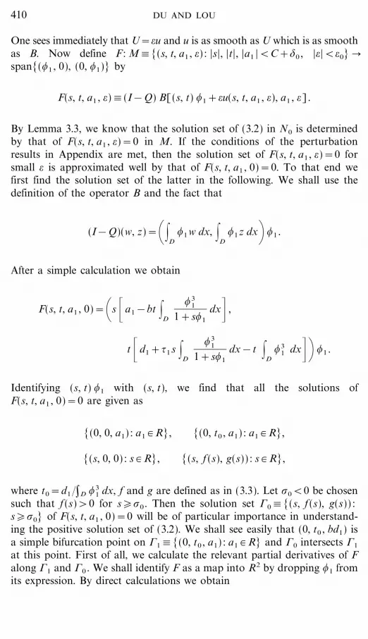
One sees immediately that U==u and u is as smooth as U which is as smoothas B. Now define F: M#[(s, t, a1 , =) : |s|, |t|, |a1 |<C+$0 , |=|<=0] �span[(,1 , 0), (0, ,1)] by
F(s, t, a1 , =)#(I&Q) B[(s, t) ,1+=u(s, t, a1 , =), a1 , =].
By Lemma 3.3, we know that the solution set of (3.2) in N0 is determinedby that of F(s, t, a1 , =)=0 in M. If the conditions of the perturbationresults in Appendix are met, then the solution set of F(s, t, a1 , =)=0 forsmall = is approximated well by that of F(s, t, a1 , 0)=0. To that end wefirst find the solution set of the latter in the following. We shall use thedefinition of the operator B and the fact that
(I&Q)(w, z)=\|D,1 w dx, |
D,1z dx+ ,1 .
After a simple calculation we obtain
F(s, t, a1 , 0)=\s _a1&bt |D
,31
1+s,1
dx& ,
t _d1+{1 s |D
,31
1+s,1
dx&t |D
,31 dx&+ ,1 .
Identifying (s, t) ,1 with (s, t), we find that all the solutions ofF(s, t, a1 , 0)=0 are given as
[(0, 0, a1) : a1 # R], [(0, t0 , a1) : a1 # R],
[(s, 0, 0) : s # R], [(s, f (s), g(s)) : s # R],
where t0=d1 ��D ,31 dx, f and g are defined as in (3.3). Let _0<0 be chosen
such that f (s)>0 for s�_0 . Then the solution set 10#[(s, f (s), g(s)) :s�_0] of F(s, t, a1 , 0)=0 will be of particular importance in understand-ing the positive solution set of (3.2). We shall see easily that (0, t0 , bd1) isa simple bifurcation point on 11#[(0, t0 , a1) : a1 # R] and 10 intersects 11
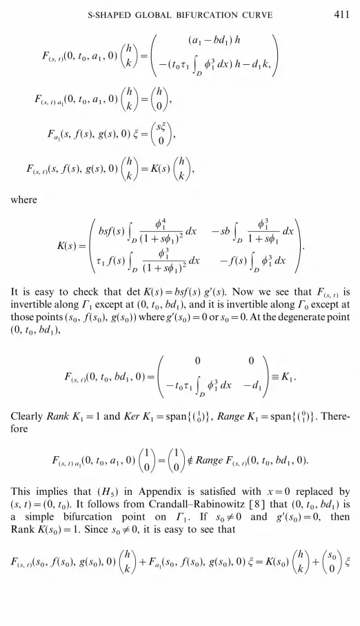
at this point. First of all, we calculate the relevant partial derivatives of Falong 11 and 10 . We shall identify F as a map into R2 by dropping ,1 fromits expression. By direct calculations we obtain
410 DU AND LOU
File: DISTL2 339422 . By:CV . Date:18:03:98 . Time:09:28 LOP8M. V8.B. Page 01:01Codes: 2600 Signs: 983 . Length: 45 pic 0 pts, 190 mm
F(s, t)(0, t0 , a1 , 0) \hk+=\
(a1&bd1) h
+&(t0 {1 |D
,31 dx) h&d1 k,
F(s, t) a1(0, t0 , a1 , 0) \h
k+=\h0+ ,
Fa1(s, f (s), g(s), 0) !=\s!
0 + ,
F(s, t)(s, f (s), g(s), 0) \hk+=K(s) \h
k+ ,
where
K(s)=\bsf (s) |
D
,41
(1+s,1)2 dx
{1 f (s) |D
,31
(1+s,1)2 dx
&sb |D
,31
1+s,1
dx
& f (s) |D
,31 dx + .
It is easy to check that det K(s)=bsf (s) g$(s). Now we see that F (s, t) isinvertible along 11 except at (0, t0 , bd1), and it is invertible along 10 except atthose points (s0 , f (s0), g(s0)) where g$(s0)=0 or s0=0. At the degenerate point(0, t0 , bd1),
F(s, t)(0, t0 , bd1 , 0)=\0 0
+#K1 .&t0{1 |
D,3
1 dx &d1
Clearly Rank K1=1 and Ker K1=span[( 10)], Range K1=span[( 0
1)]. There-fore
F(s, t) a1(0, t0 , a1 , 0) \1
0+=\10+ � Range F(s, t)(0, t0 , bd1 , 0).
This implies that (H5) in Appendix is satisfied with x=0 replaced by(s, t)=(0, t0). It follows from Crandall�Rabinowitz [8] that (0, t0 , bd1) isa simple bifurcation point on 11 . If s0{0 and g$(s0)=0, thenRank K(s0)=1. Since s0{0, it is easy to see that
F(s, t)(s0 , f (s0), g(s0), 0) \hk++Fa1
(s0 , f (s0), g(s0), 0) !=K(s0) \hk++\s0
0 + !
411S-SHAPED GLOBAL BIFURCATION CURVE

File: DISTL2 339423 . By:CV . Date:18:03:98 . Time:09:28 LOP8M. V8.B. Page 01:01Codes: 3201 Signs: 2017 . Length: 45 pic 0 pts, 190 mm
is onto. Since any square matrix is a Fredholm operator of index zero, wefind that (H3) in Appendix is satisfied along 10 except at (0, f (0), g(0))=(0, t0 , bd1). This last fact will be needed in proving Lemma 3.5 below.
Now define z(=) to be the unique positive solution of &2z=*1z+=z(d1&z), z | �D=0 for =>0. Clearly, z(=)=%*1+=d1
�=. If we define z(0)=t0 ,1 , then it is easy to use a local bifurcation argument to show that= � z(=) is C� (in fact analytic) and can be extended smoothly to =<0 butclose to 0. By the proof of Lemma 3.3, the solution (w, z)=(0, z(=)) of (3.2)can be written in the form (0, z(=))=((0, t(=)) ,1+=u(0, t(=), a1 , =), where= � t(=) is C� and t(0)=t0 . Hence (H4) is satisfied with x(=)=(0, t(=))(recall that we replaced x=0 there by (s, t)=(0, t0)). Clearly (H1) issatisfied with p=�. Thus by Proposition A.5, we obtain the followingresult.
Lemma 3.4. There exist a small neighborhood U0 of (0, t0 , bd1 , 0) in R4
and a small positive number $0 such that
F &1(0) & U0=[(s, t0+sz(s, =), a1(s, =), =) : s, = # (&$0 , $0)]
_ [(0, t(=), a1 , =) # U0],
where (s, =) � z(s, =) and (s, =) � a1(s, =) are C�, and z(0, 0)=0, a1(0, 0)=bd1 .
We see that (s, t0+sz(s, 0), a1(s, 0))=(s, f (s), g(s)), and we assume that(s, f (s), g(s), =) # U0 for |s|�s0 and |=|<$0 . Now for any C>0 defineT=[(s, f (s), g(s)) : s0�s�C]. Clearly T is compact and connected. Thefollowing result follows directly from Proposition A.3.
Lemma 3.5. There is some =0==0(C )>0, a neighborhood V of T and aC� map S : (s0 �2, C+1)_(&=0 , =0) � R3 such that S(s, 0)=(s, f (s), g(s))and all the solutions of F(s, t, a1 , =)=0 in V_(&=0 , =0) are given by
[(S(s, =), =) : |=|<=0 , s # (s0 �2, C+1)] & V_(&=0 , =0).
It is easy to see that for any |=|<=1=min($0 , =0),
1 =0=[(s, t0+sz(s, =), a1(s, =), =) : s # (&$0 , $0)]
_ [(S(s, =), =) : s # (s0�2, C+1)] & V
is a smooth curve: the two curves in the right side join somewhere in[(s, t, a1) : (s, t, a1 , =) # U0]"[(0, t0 , bd1)] and coincide in an open setthere. By the proof of Proposition A.3, we see that we can extend the func-tion S to obtain a unified parameterization of
1 =0=[(S(s, =), =) : s # (&s1 , C+1)] , (3.8)
412 DU AND LOU

File: DISTL2 339424 . By:CV . Date:18:03:98 . Time:09:28 LOP8M. V8.B. Page 01:01Codes: 2972 Signs: 1926 . Length: 45 pic 0 pts, 190 mm
where s1>0 and the function S is C� with S(s, 0)=(s, f (s), g(s)). Thislast property of S comes from the way the unified parameterization isconstructed in the proof of Proposition A.3 and the fact that theparameterizations in Lemmas 3.4 and 3.5 possess this property. To sum-marize, we have the following result.
Proposition 3.6. There exist s1 small and positive, a neighborhood VC ofTC=[(s, f (s), g(s)) : &s1 �2�s�C] and a small positive number =C suchthat for any fixed = # (&=C , =C), the solutions of F(s, t, a1 , =)=0 in VC formtwo smooth curves: 1 =
0 & VC and 1 =0 & VC , where 1 =
0 is defined as in (3.8)and 1 =
0[(0, t0+t(=), a1) : a1 # R] is given in Lemma 3.4. Moreover, this twocurves intersect at some point S(s(=), =), where = � S(s(=), =) is smooth andS(s(0), 0)=(0, t0 , bd1).
Note that S(s(=), =) corresponds to the bifurcation point (w, v, a)=(0, %d , *1(b%d)) of (1.3). By the change of variables (3.1), it is easy to seethat S(s(=), =)=(0, t(=), a1(=)), where
t(=)==&1 |D
%*1+d1= ,1 dx, a1(=)==&1[*1(b%*1+d1=)&*1].
Now we go back to problem (3.2). Clearly for any =>0, 1 =0 corresponds
to the semi-trivial solution branch [(0, z(=), a1) : a1 # R] of (3.2). It is alsoeasy to see that S((s(=), C+1), =)/1 =
0 gives a branch of positive solutionsof (3.2):
1 =(C )#[(w, z, a1)=((s, t) ,1+=u(s, t, a1 , =), a1) : (s, t, a1)
# S((s(=), C+1), =)].
We need some a priori estimates for positive solutions of (3.2) in orderto use Proposition 3.6.
Lemma 3.7. For any a01>0, there exist C0>0 and =0>0 such that any
positive solution (w, z) of (3.2) with = # (0, =0) and a1�a01 can be written as
(w, z)=(s, t) ,1+=u(s, t, a1 , =) with (s, t, a1) # VC0, where VC is defined in
Proposition 3.6.
Proof. It suffices to show that there exists C0>0 such that if (wn , zn)is a positive solution of (3.2) with a1=an
1�a01 and ===n � 0, then
(wn , zn)=(sn , tn) ,1+=n u(sn , tn , an1 , =n), and there is a subsequence of [sn]
still denoted by [sn] such that sn � s # [&s1 �2, C0], tn � f (s) andan
1 � g(s).
413S-SHAPED GLOBAL BIFURCATION CURVE

File: DISTL2 339425 . By:CV . Date:18:03:98 . Time:09:28 LOP8M. V8.B. Page 01:01Codes: 2656 Signs: 1345 . Length: 45 pic 0 pts, 190 mm
Since =zn�%*1+d1=+{1= and %*�(*&*1) � ,1 ��D ,31 uniformly in D as
* � *1+, we see easily that for all large n,
zn�1+(d1+{1) ,1<|D,3
1 .
Then it follows from the equation of wn that
*1+=n an1=*1(=nbzn �(1+wn))<*1(=nb &zn &�)
=*1+=n b &zn &��*1+=nb _1+(d1+{1) &,1&�<|D,3
1 & . (3.9)
Hence [an1] is bounded, and thus we may assume that an
1 � a1�a01>0. By
a simple regularity argument, it is easy to see from the equations in (3.2)that wn�&wn&� � ,1 �&,1 &� and zn�&zn&� � ,1 �&,1&� in C 1 norm. Since[&zn&�] is bounded, we may assume that &zn&� �&,1&� � t�0 and thuszn � t,1 in C1.
Next we show that there is some C0>0 such that &wn &�<C0 for all n.If not, we may assume that &wn&� � �. Multiplying the equation for wn
in (3.2) by ,1 and integrating we obtain
|D
,1wn(an1&bzn�(1+wn))=0. (3.10)
Dividing (3.10) by &wn&� and passing to the limit we deduce that an1 � 0,
which is impossible. Thus [&wn&�] is bounded and we may assume that&wn&��&,1&� � s�0, which implies that wn � s,1 . Therefore for all largen, (wn , zn , an
1 , =n) belongs to some N0 as defined in Lemma 3.3. ByLemma 3.3, we must have (wn , zn)=(sn , tn) ,1+=nu(sn , tn , an
1 , =n). More-over, we have sn � s and tn � t. Multiplying the equation for zn in (3.2) by,1 and integrating, we obtain
|D
,1zn(d1+{1wn�(1+wn)&zn)=0. (3.11)
Passing to the limits in (3.10) and (3.11) we get
|D
s(a1&bt,1 �(1+s,1)) ,21=0,
(3.12)
|D
t(d1+{1s,1 �(1+s,1)&t,1 ) ,21=0.
414 DU AND LOU
File: DISTL2 339426 . By:CV . Date:18:03:98 . Time:09:28 LOP8M. V8.B. Page 01:01Codes: 3033 Signs: 1904 . Length: 45 pic 0 pts, 190 mm
From (3.9) we also find that &zn&��an1 �b�a0
1 �b, which implies that t>0.It then follows easily from (3.12) that t= f (s) and a1= g(s) if s{0; if s=0,by (3.12) we see that t=d1 ��D ,3
1= f (0). We can again use *1+=nan1=
*1(=nbzn�(1+wn)) to obtain
a1= limn � �
[*1(=nbzn�(1+wn))&*1]�=n=bt |D
,31=bd1= g(0).
Hence we always have (sn , tn , an1) � (s, f (s), g(s)) for some s # [0, C0].
This finishes the proof. K
Now we can use Proposition 3.6 to conclude the following.
Proposition 3.8. For any a01>0, there exist C0>0 and =0>0 such that
any positive solution (w, z, a1) of (3.2) with a1�a01 and = # (0, =0) belongs to
1 =(C0) defined before.
Next we consider the case where a1 is small.
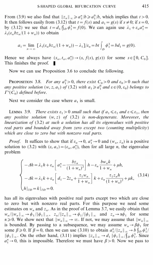
Lemma 3.9. There exists =1>0 small such that if a1�=1 and =�=1 , thenany positive solution (w, z) of (3.2) is non-degenerate. Moreover, thelinearization of (3.2) at such a solution has all its eigenvalues with positivereal parts and bounded away from zero except two (counting multiplicity)which are close to zero but with nonzero real parts.
Proof. It suffices to show that if =n � 0, an1 � 0 and (wn , zn) is a positive
solution to (3.2) with (=, a1)=(=n , an1), then for all large n, the eigenvalue
problem
{&2h=*1h+=n _an
1&bzn
(1+wn)2& h&=nbwn k
1+wn++h,
(3.14)&2k=*1k+=n _d1&2zn+
{1wn
1+wn& k+=n{1znh
(1+wn)2++k,
h | �D=k | �D=0.
has all its eigenvalues with positive real parts except two which are closeto zero but with nonzero real parts. For this purpose we need someestimates on wn and zn . As in the proof of Lemma 3.7, we easily obtain thatwn�&wn &� � ,1 �&,1&� , zn�&zn &� � ,1 �&,1 &� and zn � :,1 for some:�0. We show next that &wn&� � �. If not, we may assume that &wn&�
is bounded. By passing to a subsequence, we may assume wn � ;,1 forsome ;�0. If ;=0, then we can use (3.10) to obtain an
1 �&zn&� � b �D ,31 �
&,1&� . On the other hand, (3.11) implies &zn&� � d1 &,1 &� ��D ,31 . Since
an1 � 0, this is impossible. Therefore we must have ;>0. Now we pass to
415S-SHAPED GLOBAL BIFURCATION CURVE

File: DISTL2 339427 . By:CV . Date:18:03:98 . Time:09:28 LOP8M. V8.B. Page 01:01Codes: 3142 Signs: 2001 . Length: 45 pic 0 pts, 190 mm
the limit in (3.10) to obtain :=0, and then passing to the limit in (3.11)yields
d1=&|D
{1 ;,31 �(1+;,1)<0.
Again we arrive at a contradiction. Therefore we have &wn&� � �. Thus&zn&��&wn &� � 0 and by (3.11) we obtain :=(d1+{1)�� ,3
1 .With these properties of wn and zn , we see that (3.14) is a regular pertur-
bation of the problem
&2h=*1h++h, &2k=*1 k++k, h | �D=k | �D=0. (3.15)
Since (3.15) has 0 as a double eigenvalue with eigenspace span[(0, ,1),(,1 , 0)], and all the other eigenvalues are bounded away from 0 withpositive real parts, it follows from [22] that for all large n, (3.14) hasexactly two eigenvalues (counting multiplicity) +1
n , +2n which are close to 0,
and all the other eigenvalues are bounded away from 0 and have positivereal parts. We are going to show that these two eigenvalues both have non-zero real parts. Let +n denote either +1
n or +2n and (hn , kn) be the corres-
ponding eigenvector with &hn&2+&kn&2=1. Since +n � 0, it is easy to seefrom (3.14) that subject to choosing a subsequence, hn � !,1 and kn � ',1
in L2 for some real numbers ! and ' satisfying |!|+|'|=1. There are twopossibilities: (i) '{0, (ii) '=0. In case (i), we can assume that '>0 by asimple rescaling of the eigenvectors. Then we multiply the equation for kn
in (3.14) by ,1 , integrate it, divide it by =n and pass to the limit to obtain
d1 '&2:' |D
,31+{1'+' lim
n � �+n �=n=0. (3.16)
Hence +n�=n � d1+{1 . Now we do the same thing to the equation of hn
and obtain !+n �=n � b'. Therefore !=b'�(d1+{1) and thus '=(d1+{1)�(b+d1+{1).
In case (ii), we have kn � 0 in L2. We may assume that hn � ,1 . By usingthe equation of hn we easily see that +n�=n � 0. Now we decompose kn askn='n ,1+k$n, �D ,1k$n=0. From the equation of kn we obtain
&k$n&2�=nM &(d1&2zn+{1 wn�(1+wn)++n) kn&2+=nM " {1zn hn
(1+wn)2"2
�=nM1(&kn &2+1�&wn &2�), (3.17)
where M is the norm of (&2&*1)&1 from the orthogonal complement ofspan[,1] in L2 to L2. By passing to a subsequence, we have either &k$n&2=o(1�&wn&�
2) or &k$n&2=o(&kn&2) and hence kn�'n � ,1 in L2. If the latter
416 DU AND LOU

File: DISTL2 339428 . By:CV . Date:18:03:98 . Time:09:28 LOP8M. V8.B. Page 01:01Codes: 2875 Signs: 1655 . Length: 45 pic 0 pts, 190 mm
happens, then we multiply the equation for kn by ,1 , integrate it, divide itby 'n=n and pass to the limit to find that
|D
(d1&2:,1+{1) ,21+ lim
n � �(:{1 &,1&2
�)�('n&wn&2�)=0.
That is,
'n &wn &2� � :{1 &,1&2
��(d1+{1).
Then it follows that &kn&2=O(1�&wn &2�) which implies that we always
have &kn&2=O(1�&wn&2�). Now, using (3.10) we can easily deduce
an1 &wn&� � : &,1&� . Finally we multiply the equation of hn by ,1 ,
integrate it, divide it by =n�&wn &� , and obtain by passing to the limit that
limn � �
&wn&� +n�=n=& limn � �
an1 &wn &�=&: &,1&�<0.
Hence for large n, either (hn , kn) is close to (b,1 �b+d1+{1 , (d1+{1) ,1 �b+d1+{1 ) and +n�=n is close to d1+{1>0, or (hn , kn) is close to (,1 , 0)and &wn&� +n�=n is close to &(d1+{1) &,1 &��� ,3
1<0. K
Proposition 3.10. There exists =2>0 small such that for any a1 , = # (0, =2],(3.2) has a unique positive solution. Moreover, the positive solution isnon-degenerate and unstable. By the Implicit Function Theorem, the positivesolutions [(w, z, a1) : a1 # (0, =2]] form a smooth curve 1� = parameterized bya1 and it varies smoothly with =.
Proof. Let =1>0 be given by Lemma 3.9. Then we know that everypositive solution (w, z) of (3.2) with =, a1 # (0, =1] is non-degenerate. Oneeasily checks that
g(0)=bd1<|D,3
1 ,
lims � �
sg(s)=(d1+{1) b<| ,31>0, (3.18)
lims � �
s2g$(s)=&(d1+{1) b<| ,31<0.
Therefore we can find S0>0 large such that g(S0)<=1 , g$(s)<0 fors�S0&1 and g(s)>g(S0) for 0<s<S0 . We show next that there exists=2 # (0, =1) such that for each a1 # [ g(2S0), g(S0)] and = # (0, =2], (3.2) hasa unique positive solution. This follows easily from Proposition 3.8. In fact,if (w, z) is a positive solution of (3.2) with a1 # [ g(2S0), g(S0)] and = small,
417S-SHAPED GLOBAL BIFURCATION CURVE

File: DISTL2 339429 . By:CV . Date:18:03:98 . Time:09:28 LOP8M. V8.B. Page 01:01Codes: 3303 Signs: 2472 . Length: 45 pic 0 pts, 190 mm
then (w, z, a1) # 1 =(C0), and if we express S(!, =) in the form S(!, =)=(s(!, =), t(!, =), a1(!, =)), then (s(!, 0), t(!, 0), a1(!, 0))=(!, f (!), g(!)).Since g$(!)<0 for ! # [S0&1, 2S0+1], we can find some =2>0 so that for= # (0, =2], �a1(!, =)��!<0 for ! # [S0&1, 2S0+1] and [ g(2S0), g(S0)]/a1([S0&1, 2S0+1], =). Thus for each a1 # [ g(2S0), g(S0)], there is aunique !=!(a1 , =) such that a1=a1(!(a1 , =), =). This shows that there isexactly one positive solution of (3.2) for = # (0, =2] and a1 # [ g(2S0),g(S0)].
Uniqueness for a1 # (0, g(2S0)] now follows easily by using Lemma 3.9,Proposition 3.8 and a simple continuation argument. Note that the positivesolution set [(w, z, a1)] of (3.2) for a1>0 bounded away from 0 and anyfixed =>0 is precompact.
Next we consider the stability of the unique positive solution. By Lemma3.9, and the Leray�Schauder formula for fixed point index, any such solu-tion (w, z) of (3.2) would have fixed point index 1 unless exactly one of thesmall eigenvalues of the linearization of (3.2) at (w, z) has negative realpart (and hence both small eigenvalues are real). But, as in the last part ofthe proof of Lemma 2.6, the unique positive solution has fixed point index&1 by the additivity of the degree, since the total degree of the nonnegativesolutions is 0 and the degree of the only semi-trivial solution (0, z) is 1.Hence it must be unstable (the linearization at it has exactly one negativeeigenvalue, counting multiplicity). This finishes the proof. K
Proof of Theorem 3.1. It is clear that 1 ==1� = _ 1 =(C0) is a smoothcurve which varies smoothly with = for all small positive =. CombiningPropositions 3.8 and 3.10, we immediately obtain Theorem 3.1. K
3.2. Further Analysis of the Global Solution Curve
In this subsection, we look more carefully at the solution curve 1 =. Wefirst analyze the stability of the solutions (w, z, a1)=(w(s, =), z(s, =),a1(s, =)). Note that if S(!, =)=(s(!, =), t(!, =), a1(!, =)), then
(w(!, =), z(!, =))=((s(!, =), t(!, =)) ,1+=u(s(!, =), t(!, =), a1(!, =), =)).(3.19)
The linearization problem of (3.2) at the positive solution (w, z)=(w(s, =),z(s, =)) with a1=a1(s, =) can be written as
L(s, =)(h, k)#&H(h, k)&=B(w, z)(w(s, =), z(s, =), a1(s, =))(h, k)=+(h, k).
As in the proof of Lemma 3.9, L(s, =) is a small perturbation of H. Thenit follows from [22] that for small =>0, all the eigenvalues of L(s, =) arebounded away from zero and with positive real parts except two which areclose to zero. Denote these two small eigenvalues by +1(s, =) and +2(s, =).
418 DU AND LOU

File: DISTL2 339430 . By:CV . Date:18:03:98 . Time:09:28 LOP8M. V8.B. Page 01:01Codes: 3122 Signs: 1938 . Length: 45 pic 0 pts, 190 mm
Then clearly the stability of (w(s, =), z(s, =)) is completely determined by+1(s, =) and +2(s, =).
Proposition 3.11. Let +1(s0) and +2(s0) be the two eigenvalues of K(s0),then
lim(s, =) � (s0 , 0)
+i(s, =)�==&+i (s0), i=1, 2. (3.20)
Proof. We divide the proof into two cases: (i) +1(s0){+2(s0), (ii)+1(s0)=+2(s0). We consider case (i) first. In this case we give a constructiveproof which will be useful later in the discussion of Hopf bifurcations. Wewant to solve the equation
L(s, =)(h, k)=+(h, k) (3.21)
for (h, k, +) with (h, k){(0, 0). If we can find solutions (h1 , k1 , +1) and(h2 , k2 , +2) such that (h1 , k1) and (h2 , k2) are linearly independent and+1 , +2 are close to 0, then we necessarily have +1(s, =)=+1 , +2(s, =)=+2 .
In the rest of the proof, we understand that the spaces X, Y, X1 , Y1 andspan[(,1 , 0), (0, ,1)] are all Banach spaces of complex valued functionsover the complex field C. Suppose that P and Q are the projections of thecomplex spaces X onto X1 and Y onto Y1 respectively. Then we look forsolutions (h, k, +) to (3.21) with the following form:
+==`, (h, k)=(1, ') ,1+=V, V # X1 .
Under these change of variables, (3.21) is equivalent to
{QH(V )+QB� (s, =)[(1, ') ,1+=V ]&=`V=0,(I&Q) B� (s, =)[(1, ') ,1+=V ]&`(1, ') ,1=0,
(3.22)
where B� (s, =)=B(w, z)(w(s, =), z(s, =), a1(s, =)). Now let N be a small neighbor-hood of (s0 , 0) in R2, and define G=(G1 , G2), where G1 : C_X1_C_N �span[(,1 , 0), (0, ,1)] and G2 : C_X1_C_N � Y1 are given by
{G1(', V, `, s, =)=(I&Q) B� (s, =)[(1, ') ,1+=V]+`(1, ') ,1 ,G2(', V, `, s, =)=QH(V )+QB� (s, =)[(1, ') ,1+=V]+=`V.
(3.23)
Then clearly G( 'i , Vi , &+ i ( s0 ), s0 , 0) = 0, i = 1, 2, where (1, 'i) is aneigenvector of K(s0) corresponding to the eigenvalue +i (s0), and Vi=(QH )&1 QB� (s0 , 0)[( 1
'i) ,1]. Note that since all the entries in K(s0) are non-
zero, any eigenvector of K(s0) must have both components nonzero. There-fore we can always choose the eigenvector to be of the form (1, '). Fori=1, 2, let Ai=G(', V, `)('i , Vi , &+i (s0), s0 , 0). A direct calculation shows
419S-SHAPED GLOBAL BIFURCATION CURVE

File: DISTL2 339431 . By:CV . Date:18:03:98 . Time:09:28 LOP8M. V8.B. Page 01:01Codes: 3130 Signs: 1805 . Length: 45 pic 0 pts, 190 mm
Ai (', V, `)=((I&Q) B� (s0 , 0)[(0, ') ,1]&+i (s0)(0, ') ,1+`(1, 'i) ,1),
QH(V )+QB� (s0 , 0)[(0, ') ,1]).
Since (I&Q) B� (s0 , 0)=K(s0) has two different eigenvalues, it is easy to seethat Ai is 1-1 and onto. Therefore it follows from the Implicit FunctionTheorem that for any (s, =) near (s0 , 0), G(', V, `, s, =)=0 has a uniquesolution (', V, `)=('i (s, =), Vi (s, =), `i (s, =)), where the functions aresmooth and 'i (s0 , 0)='i , Vi (s0 , 0)=Vi , `i (s0 , 0)=&+i (s0). Note that thetwo eigenfunctions of L(s, =) obtained in this way must be linearly inde-pendent as the corresponding eigenvalues are different. This finishes theproof for case (i).
Next we consider case (ii). We use an argument along the lines of theproof of Lemma 3.9. It suffices to show that if (wn , zn , an
1)=(w(sn , =n),z(wn , =n), a1(sn , =n)), sn � s0 , =n � 0, (hn , kn , +n) is a nontrivial solution to(3.14) with &hn&2+&kn&2=1 and +n � 0, then, by choosing a subsequence,for all large n, +n�=n is close to &+1(s0)=&+2(s0). Note that, sinceL(sn , =n) is real, +� n is always an eigenvalue of L(sn , =n) if +n is. As in theproof of Lemma 3.9, by passing to a subsequence, we have hn � :,1 , kn �;,1 , where |:|+|;|=1. Note that now we have wn � s0,1 , zn � f (s0) ,1 ,an
1 � g(s0). Hence multiplying the equation for hn by ,1 , integrating over D,dividing by =n and then passing to the limit we obtain
: _g(s0)&|D
bf (s0) ,31 �(1+s0,1)2+ lim
n � �+n �=n&
&; |D
bs0,31 �(1+s0,1)=0,
that is,
: _bf (s0) s0 |D
,41 �(1+s0,1)2+ lim
n � �+n�=n&
&; _bs0 |D
,31�(1+s0 ,1)&=0. (3.24)
Doing the same to the equation for kn we obtain, after some simplifica-tions,
; _&2f (s0) |D
,31+ lim
n � �+n �=n&+: _{1 f (s0) |
D,3
1 �(1+s0,1)2&=0.
(3.25)
From (3.24) and (3.25) it follows that +n�=n � +0 and &+0 is an eigenvalueof K(s0) with eigenvector (:, ;). Therefore, for all large n, &+n�=n is closeto the double eigenvalue of K(s0). This finishes the proof. K
420 DU AND LOU

File: DISTL2 339432 . By:CV . Date:18:03:98 . Time:09:28 LOP8M. V8.B. Page 01:01Codes: 2896 Signs: 1957 . Length: 45 pic 0 pts, 190 mm
From the expression of K(s), we see that its eigenvalues +1(s) and +2(s)satisfy
+1(s)++2(s)= f (s) h(s),
where
h(s)=sb |D
,41 �(1+s,1)2&|
D,3
1 , +1(s) +2(s)=bsf (s) g$(s). (3.26)
Thus by Proposition 3.11 we have the following result.
Theorem 3.12. If h(s0)>0, then for (s, =) close to (s0 , 0), (w(s, =),z(s, =), a1(s, =)) is unstable; If h(s0)<0, then for (s, =) close to (s0 , 0),(w(s, =), z(s, =), a1(s, =)) is stable if g$(s0)>0, and unstable if g$(s0)<0.
For a given a1 , the number of positive solutions is determined by thatof the solutions s to a1=a1(s, =). Since a1(s, =) is close to g(s) for small =,it reduces to analyzing the curve a1= g(s). Since g(s) is analytic andg$(s)<0 for all large s, g$(s)=0 has at most finitely many solutions: si ,0�i�k. For each si , there is an integer pi>1 such that g( pi)(si){0. Itfollows that if g$(0){0, there exists =0>0 small such that for any fixed= # (0, =0], �a1(s, =)��s=0 has exactly k positive solutions s1(=)< } } } <sk(=), and � pia(si (=), =)��s pi{0. Denote (wi , zi , ai
1)=(w(si (=), =), z(si (=), =),a1(si (=), =)), i=1, ..., k. Then we are ready to state and prove the followingresult.
Theorem 3.13. Suppose that g$(0){0. Then there exists =0>0 smallsuch that for = # (0, =0], (wi , zi , ai
1) defined above are exactly all thedegenerate positive solutions of (3.2). The positive solution curve 1 = given inTheorem 3.1 is divided into k+1 pieces of smooth curves by these kdegenerate points on it:
1 ="[(wi , zi , ai1) : 1�i�k]= .
k+1
i=1
1 =(i).
On each 1 =(i), the positive solutions are non-degenerate and can beparameterized by a1 . Moreover, there exists b
�>0 such that if b<b
�, then the
solutions in each 1 =(i) are either all stable, or all unstable, and no Hopfbifurcation can occur along 1 =.
To prove Theorem 3.13, we need the following result.
Lemma 3.14. For any given $0>0, there exists =0>0 such that if= # (0, =0], then the linearization of (3.2) at any positive solution (w, z) with&w&W2, 2�$0 satisfies condition (H3).
421S-SHAPED GLOBAL BIFURCATION CURVE

File: DISTL2 339433 . By:CV . Date:18:03:98 . Time:09:28 LOP8M. V8.B. Page 01:01Codes: 3388 Signs: 2348 . Length: 45 pic 0 pts, 190 mm
Proof. It suffices to show that if =n � 0, and if (wn , zn , an1) is a degenerate
solution of (3.2) with ===n , then for all large n, dim Ker(Ln)=codim Range(Ln)=1, and (wn , 0)�Range(Ln), where Ln=H+=nB(w, z)(wn , zn , an
1). By Pro-positions 3.8 and 3.10, we see immediately that (wn , zn , an
1)=(w(sn , =n),z(sn , =n), a1(sn , =n)) for some sn # (s(=n), C0]. By passing to a subsequence,we may assume that sn � s0 . Since &wn &W 2, 2�$0 , we must have s0>0. ByProposition 3.11, we know that the two small eigenvalues +n
i =+i (sn , =n),i=1, 2 of Ln are such that +n
1 �=n � &+1(s0), +n2 �=n � &+2(s0). By our
assumption, one of the small eigenvalues must be zero. Let +n1=0. Then
+1(s0)=0. Since all the entries of K(s0) are nonzero, +1(s0)=0 cannot bea double eigenvalue. Hence +2(s0) must be a nonzero real eigenvalue. Let(1, '2) be an eigenvector corresponding to +2(s0) (recall that any eigen-vector of K(s0) must have both components nonzero). By the proof of case(i) in Proposition 3.11, we can choose the eigenvector (hn , kn) of Ln corre-sponding to +n
2 such that it converges to (1, '2) ,1 . Since +n2{0 for large
n and is real, (hn , kn)=Ln(hn�+n2 , kn �+n
2) is in the range of Ln . Now we seeeasily that (hn , kn) � X1 , span[(hn , kn)]�X1/Range(Ln). Since Ln : X � Yis a compact perturbation of H : X � Y (note that X embeds compactlyinto Y ), and H is a Fredholm operator of index 0, Ln must be of Fredholmwith index 0. But by assumption and the previous discussion, dim Ker(Ln)=1.Therefore we necessarily have Range(Ln)=span[(hn , kn)]�X1 .
It remains to show that (wn , 0) � Range(Ln). Suppose that this is nottrue. Then we can write
(wn , 0)=:n(hn , kn)+(un , vn), |D
un,1=|D
vn,1=0.
It follows then
|D
wn,1=:n |D
hn ,1 , 0=:n |D
kn,1 .
Passing to the limits, we obtain :n � s0>0 and :n � 0 respectively. Thiscontradiction finishes our proof. K
Proof of Theorem 3.13. By Propositions A.5 and A.5$ we can find aneighborhood N0 of (0, f (0) ,1 , g(0) ,1) such that 1 = & N0 contains onlynon-degenerate solutions for small =. Then by Lemma 3.14 and a result ofCrandall�Rabinowitz, we know that if (w0 , z0 , a0
1) is a degenerate positivesolution to (3.2) with =>0 small, then there is a neighborhood N of thispoint such that all the solutions of (3.2) in N forms a smooth curve andthis curve can not be parameterized by a1 near (w0 , z0 , a0
1). On the otherhand, we must have (w0 , z0 , a0
1)=(w(s0 , =), z(s0 , =), a1(s0 , =)) for some s0 .
422 DU AND LOU

File: DISTL2 339434 . By:CV . Date:18:03:98 . Time:09:28 LOP8M. V8.B. Page 01:01Codes: 2965 Signs: 1753 . Length: 45 pic 0 pts, 190 mm
Thus we necessarily have �a1(s0 , =)��s=0. Hence s0=si (=) and (w0 , z0 , a01)=
(wi , zi , ai1) for some 1�i�k. Conversely, (wi , zi , ai
1), i=1, ..., k are alldegenerate solutions of (3.2): otherwise, by the Implicit Function Theorem,all the nearby solutions of (3.2) form a smooth curve which can be para-meterized by a1 , i.e., the nearby parts of 1 = can be parameterized by a1 .But this contradicts the fact that �a1(si (=), =)��s=0. Let
b�=| ,3
1<_ maxs # [0, �) | s,4
1 �(1+s,1)2& . (3.27)
Clearly, h(s)<0 for s # [0, �) if b�b�. This implies that +1(s)++2(s)<0
for all s�0. By Proposition 3.11 we see that the two small eigenvalues ofthe linearization of (3.2) along 1 =(C0) can never be a pure imaginary pair.This finishes the proof. K
Remark 3.15. If for some fixed i, g$(s)<0 for s # (si , si+1), then clearly+1(s) and +2(s) cannot be a conjugate complex pair. Then the same reason-ing as in the last part of the above proof shows that Hopf bifurcation doesnot occur along the corresponding 1 =(i+1) when =>0 is small.
Next we show that for large b and suitable choices of d1 and {1 , Hopfbifurcation along the solution curve 1 = of (3.2) can occur for any small=>0. More precisely,
Theorem 3.16. Let d1 , {1 satisfy {1 �d1�2 �D ,41 �(�D ,3
1 )2. Then thereexists some positive constant b� >0, depending only on D, such that if b�b� ,for any small =>0, Hopf bifurcation occurs along the positive solution curve1 = of (3.2).
Proof. It is easy to check that
g$(s)b |
D,3
1=&d1 |D
,41
(1+s,1)2+{1 |D
,31
1+s,1
__|D
,31
1+s,1
&2s |D
,41
(1+s,1)2& ,
h$(s)�b=|D
,41
(1+s,1)2&2s |D
,51
(1+s,1)2 .
Let {1�d1�2 �D ,41 �(�D ,3
1)2. It is easy to see that there exists $0>0 small,independent of b, d1 and {1 , such that if s # [0, $0], then g$(s)>0 andh$(s)>0. Set
b� = mins # (0, $0] |
D,3
1<\s |D
,41 �(1+s,1)2+ . (3.28)
423S-SHAPED GLOBAL BIFURCATION CURVE

File: DISTL2 339435 . By:CV . Date:18:03:98 . Time:09:28 LOP8M. V8.B. Page 01:01Codes: 2963 Signs: 1845 . Length: 45 pic 0 pts, 190 mm
Hence for any b�b� , there exists some s0 # (0, $0] such that
bs0 |D
,41 �(1+s0,1)2=|
D,3
1 ,
(3.29)
bs |D
,41 �(1+s,1)2<|
D,3
1 , s # (0, s0).
Summarizing the above discussions we have
g$(s0)>0, h(s0)=0, h$(s0)>0, h(s)<0, s # (0, s0). (3.30)
It follows from (3.26) that the two eigenvalues of K(s0) are given by
+1(s0)=i;0 , +2(s0)=&i;0 , ;0=- bs0 f (s0) g$(s0)>0.
It follows then from bifurcation theory for linear operators (see, e.g., [22])that for s near s0 , the two eigenvalues of K(s) are conjugate complex pairs:
+1(s)=:(s)+i;(s), +2(s)=:(s)&i;(s),
where : and ; are smooth functions and :(s0)=0, ;(s0)=;0 . We also have:$(s0)= f (s0) h$(s0)�2>0. Now we use Proposition 3.11 to find that for(s, =) close to (s0 , 0), the two small eigenvalues +1(s, =) and +2(s, =) of thelinearization of (3.2) about (w, z) at (w(s, =), z(s, =), a1(s, =)) are conjugatecomplex pairs, and both are simple eigenvalues. It then follows from resultson simple eigenvalues that
+1(s, =)=:(s, =)+i;(s, =), +2(s, =)=:(s, =)&i;(s, =),
where : and ; are smooth functions. By the proof of case 1 of Proposition3.11, we must have +i (s, =)==`i (s, =) for all s close to s0 and positive small=, where `i (s, =) is smooth for all s close to s0 and all (not necessarilypositive) = close to 0, and `i (s, 0)=+i (s). Thus we can find =0>0 smallsuch that for any = # (0, =0], there is a unique s= # (s0&=0 , s0+=0) such that:(s= , =)=0, :$s(s= , =)>0, and ;(s, =){0 for s # (s0&=0 , s0+=0). Therefore,Hopf bifurcation occurs at (w, z, a1)=(w(s= , =), z(s= , =), a1(s= , =)) (see, e.g.,[7, 20]). K
Remark 3.16$. In view of Theorem 3.12 and (3.30), it is easy to see thatthe positive solution (w(s, =), z(s, =)) loses stability as s passes through s= .Note that g$(s)>0 for s<s= . Therefore for =>0 small, s � a1(s, =) isincreasing for s<s= . This fact will be needed in proving part (iii) ofTheorem 4.1. It seems possible to use the method presented in [20] to
424 DU AND LOU

File: DISTL2 339436 . By:CV . Date:18:03:98 . Time:09:28 LOP8M. V8.B. Page 01:01Codes: 3184 Signs: 2144 . Length: 45 pic 0 pts, 190 mm
determine the stability of the periodic solutions obtained by the Hopf bifur-cation. As the calculation seems rather tedious and long, we do not pursueit here. We suspect that the periodic solutions are stable.
Finally, we discuss the shape of the bifurcation curve 1 =. For small =, theproblem is reduced to analyzing the function g(s). Clearly,
g(0)=d1b<| ,31 , g(�)# lim
s � �g(s)=0.
From the expression of g$(s), one easily sees that there exists some smallpositive number $1 such that g$(s)<0 for all s�0 if {1 �d1<$1 . On theother hand, if {1 �d1>� ,4
1 �(� ,31)2, then a1*=sups # [0, �) g(s) is achieved at
some s>0 and a1*>g(0). Set
a1*(=)= maxs # [0, �)
a1(s, =)
and recall that the positive solution curve 1 = intersects the semi-trivialsolution curve [(0, z, a1)] at the point
(w(s(=), =), z(s(=) =), a1(s(=), =))=(0, =&1%*1+d1= , =&1[*1(b%*1+d=&*1]).
That is, the positive solution curve 1 = bifurcates from the semi-trivial solu-tion branch [(0, z, a1)] at a1=a1(=)#a1(s(=), =). Now by the above discus-sions we have the following result.
Theorem 3.17. There exists =0>0 small such that, for any 0<=<=0 ,the a1 range which the positive solution curve 1 = covers is (0, a1*(=)) or(0, a1*(=)]. Moreover, the a1 range is the former if {1 �d1<$1 , and in thiscase, (3.2) has a unique positive solution for any a1 # (0, a1*(=)); on the otherhand, if {1�d1>� ,4
1 �(� ,31)2, then a1*(=)>a1(=), the desired a1 range is
(0, a1*(=)], and (3.2) has at least two positive solutions for any a1 #(a1(=), a1*(=)).
From the above we see that if {1 �d1>� ,41 �(� ,3
1)2, then the curve 1 = hasat least one turning point at a1=a1*(=) and 1 = lies to the left of this point.It would be interesting to know whether there is exactly one turning point.We show in the following that this is indeed the case if {1 �d1 is large forsome special type domain D.
Theorem 3.18. Suppose that the domain D is a ball in RN with N�3, orD=[a1 , b1]_[a2 , b2]_ } } } _[aN , bN] with N�6. Then there exists $>0small, depending only on D, such that if d1 �{1�$, then g(s) has a uniquecritical point in (0, �) denoted by s0 . Moreover, g"(s0)<0. It follows that,in these cases, 1 = is exactly ``#'' shaped.
425S-SHAPED GLOBAL BIFURCATION CURVE

File: DISTL2 339437 . By:CV . Date:18:03:98 . Time:09:28 LOP8M. V8.B. Page 01:01Codes: 2087 Signs: 953 . Length: 45 pic 0 pts, 190 mm
To establish Theorem 3.18, we first prove the following lemma.
Lemma 3.19. Suppose that 8�0 is a continuous, non-negative functionin D� . If 1
|D| �D 8� 427 maxD� 8, then the function
g1(s)#s1�2 |D
83�(1+s8) dx, s # (0, �)
has a unique critical point.
Proof. Without loss of generality we may assume that maxD� 8=1. It iseasy to check that
2s1�2g$1(s)=|D
83�(1+s8)&2s |D
84�(1+s8)2,
(3.31)
2sg1"(s)+ g$1(s)=4s3�2 |D
85�(1+s8)3&3s1�2 |D
84�(1+s8)2.
Claim. If g$1(s)=0, then g1"(s)<0.
To establish this assertion, we consider two cases: (i) s<3. For this case,our assertion follows readily from (3.31) as
2sg1"(s)=s1�2 |D
84(s8&3)�(1+s8)3<0. (3.32)
(ii) s�3. For this case we argue by contradiction. Suppose that thereexists s�3 such that g$1(s)=0 and g1"(s)�0. It is easy to check thatg$1(s)=0 is equivalent to
|D
83�(1+s8)=2 |D
83�(1+s8)2. (3.33)
The assumption g$1(s)=0 and g1"(s)�0 implies that
4s |D
85�(1+s8)3�3 |D
84�(1+s8)2, (3.34)
which is the same as
|D
84�(1+s8)2�4 |D
84�(1+s8)3. (3.35)
426 DU AND LOU

File: DISTL2 339438 . By:CV . Date:18:03:98 . Time:09:28 LOP8M. V8.B. Page 01:01Codes: 2214 Signs: 1008 . Length: 45 pic 0 pts, 190 mm
Multiplying (3.35) by s and simplifying, by (3.33) we find
4 |D
83�(1+s8)3�3 |D
83�(1+s8)2. (3.36)
We can further simplify (3.36) to obtain
7 |D
82�(1+s8)2�4 |D
82�(1+s8)3+3 |D
82�(1+s8). (3.37)
By Holder and Cauchy inequalities we have
|D
82�(1+s8)2�\|D82�(1+s8)3+
1�2
\|D82�(1+s8)+
1�2
�2�3 |D
82�(1+s8)3+3�8 |D
82�(1+s8), (3.38)
which can be rewritten as
|D
82�(1+s8)3>3�2 |D
82�(1+s8)2&9�16 |D
82�(1+s8). (3.39)
Substituting (3.39) into (3.37) we obtain
4 |D
82�(1+s8)2>3 |D
82�(1+s8). (3.40)
Repeating those arguments from (3.36) to (3.40), we can similarly showthat
4 |D
8�(1+s8)>3 |D
8. (3.41)
By the elementary inequality (1+s8)�2(s8)1�2 and s>3, from (3.41) itfollows that
|D
8<2�(3 - 3) |D
81�2�2�(3 - 3) \|D8+
1�2
|D| 1�2.
That is, �D 8�|D|<4�27, which contradicts the assumption. This establishesour assertion.
As g1(0)=0 and lims � � g1(s)=0, we can conclude that g1 has at leasta critical point in (0, �). By the conclusion of the Claim and some elemen-tary argument we see that g1(s) has exactly one critical point denoted by
427S-SHAPED GLOBAL BIFURCATION CURVE

File: DISTL2 339439 . By:CV . Date:18:03:98 . Time:09:28 LOP8M. V8.B. Page 01:01Codes: 2362 Signs: 1171 . Length: 45 pic 0 pts, 190 mm
s0 . Furthermore, from the proof we see that g1"(s0)<0. It is easy to see thatg1 attains local (and thus global) maximum at s=s0 . K
Proof of Theorem 3.18. Let 8=81 in Lemma 3.19. When D=7N ,then 81 is given by
81(x)=sin[?(x1&a1)�(b1&a1)] } } } sin[?(xN&aN)�(bN&aN)].
Therefore �D 8�|D|=(2�?)N>4�27 provided that N�6. When D is a ballin R3, e.g., the unit ball, then 81(x)=sin(? |x| )�(? |x| ). Hence for this case,�D 8�|D|=4�?2>4�27. It remains to consider the case when D is a ball inR2. Without loss of generality we may assume that D is the unit ball in R2.
Claim 1. �D 81�4?�(e*1(D)).
To establish this assertion, we consider
ut=2u in D_(0, �), u | �D=0, u(x, 0)=81(x). (3.42)
Let G(t, x)=(4?t)&1 e&|x|2�(4t) be the fundamental solution of the heatequation in R2. Then we have
u(x, t)�|D
G(t, x& y) 81( y) dy�1
4?t |D81( y) dy, \x # D, t>0.
Since e&*1(D) t81(x) is the solution of (3.42), hence
4?te&*1(D) t�|D
81 , \t>0. (3.43)
The assertion now follows from (3.43) by letting t=1�*1(D).
Claim 2. If D is the unit ball in R2, then *1(D)<3+2 - 2.Set ,0(x)=1&|x|- 2. Then
*1(D)= inf,{0
�D |{,| 2
�D ,2 <�D |{,0 | 2
�D ,20
=�1
0 r(,$0)2 dr�1
0 r,20 dr
=3+2 - 2.
Now it follows from our two assertions that
�D 81
|D|=
�D 81
?�
4e*1(D)
�4
e(3+2 - 2)>
427
.
428 DU AND LOU

File: DISTL2 339440 . By:CV . Date:18:03:98 . Time:09:28 LOP8M. V8.B. Page 01:01Codes: 2935 Signs: 1948 . Length: 45 pic 0 pts, 190 mm
Therefore by Lemma 3.19 we see that g1(s) with 8=,1=81�&81&2 hasa unique critical point, and it is a strict local (global) maximum. Clearly,the function [ g1(s)]2 also has these properties. Since
g(s)=b{1
�,31 _
d1
{1|
,31
1+s,1
+ g21(s)& ,
by a simple perturbation argument we see that for d1 �{1 small, the sameconclusion holds true for g. This completes the proof of Theorem 3.18. K
4. THE MAIN RESULTS
In this section, we use results from Sections 2, 3 and the Appendix toprove our main result
Theorem 4.1. For any fixed b>0, there exists an open set O=O(b)/(0, �)_(0, �), such that for any ({, d ) # O, we can find M=M(b, d, {)large so that for each m�M :
(i) All positive solutions (u, v, a) of (1.1) lie on an unbounded smoothcurve 1 which bifurcates from the semi-trivial solution curve [(0, %d , a) :a>*1] at the point (0, %d , *1(b%d)). Moreover, 1 is roughly S-shaped: thereexist a
*=*1+O(1�- m) # (*1 , *1(b%d)) and a*>*1(b%d), both depending on
b, d, { and m, such that (1.1) has a positive solution if and only if a�a*
; ithas exactly one positive solution for a=a
*and a>a*, at least two positive
solutions for a # (a*
, *1(b%d)) _ [a*], and at least three positive solutions fora # (*1(b%d), a*).
(ii) There are at most a finite number k (�2) of degenerate positivesolutions of (1.1) which we denote by [(ui , vi , ai) : 1�i�k]. The positivesolution curve 1 given in part (i) is divided into k+1 pieces of smooth curvesby these k degenerate points on 1:
1"[(ui , vi , ai) : 1�i�k]= .k+1
i=1
1(i).
On each 1(i), the positive solutions are non-degenerate and can beparameterized by a;
(iii) There exist b� >b�>0, depending only on D, such that if b�b
�, then
the solutions in each 1(i) are either all stable, or unstable, and Hopf bifurca-tion does not occur along 1; if b�b� , then Hopf bifurcation occurs along 1(1)at some a0 # (*1(b%d), a*), where 1(1) has (0, %d , *1(b%d)) in its closure.Moreover, there are two asymptotically stable solutions if a # (*1(b%d), a0).
429S-SHAPED GLOBAL BIFURCATION CURVE

File: DISTL2 339441 . By:CV . Date:18:03:98 . Time:09:29 LOP8M. V8.B. Page 01:01Codes: 3232 Signs: 2139 . Length: 45 pic 0 pts, 190 mm
(iv) There exists a subset O1 of O such that if ({, d ) # O1 , and if thedomain D is a ball in RN with N�3, or D=[a1 , b1]_ } } } _[aN , bN] withN�6, then the curve 1 is exactly S-shaped: there are exactly two degeneratepoints on 1, and (1.1) has no positive solution for a<a
*, exactly one positive
solution for a=a*
(neutrally stable), exactly two positive solutions fora # (a
*, *1(b%d)] (one stable and one unstable), exactly three positive solu-
tions for a # (*1(b%d), a*) (two stable, one unstable if b�b�; if b�b� , then
Hopf bifurcation occurs as in part (iii) above), exactly two positive solutionsfor a=a* (one stable, one neutrally stable), and exactly one positive solutionfor a # (a*, �) (stable).
Remark 4.2. (i) The open sets O and O1 are defined as follows.
O=[(={1 , *1+=d1) : d1 �{1 # (0, 20), = # (0, =0(b, d1 , {1))],
where 20=(�D ,31 dx)2�(2 �D ,4
1 dx), ,1=81 �&81&2 , and =0(b, d1 , {1) is afunction of (b, d1 , {1) taking small positive values only;
O1=[(={1 , *1+=d1) : d1 �{1 # (0, $0), = # (0, =0(b, d1 , {1))],
where $0<20 is a small positive number depending only on D.
(ii) The numbers b�
and b� are given by (3.27) and (3.28) respectively.
Proof. Let r=1�m and (w, v)=(u�r, v), then (1.1) becomes
{2w+w(a&rw&bv�(1+w))=02v+v(d+{w�(1+w)&v)=0
in D, w | �D=0,in D, v | �D=0.
(4.1)
Define the operator F : [W 2, p & H 10]2 � [L p]2, p>N, by
F(w, v, a, r)=\ 2w+w(a&bv�(1+w))2v+v(d+{w�(1+w)&v)+&r \w2
0 + . (4.2)
It is obvious that F(w, v, a, r)=0 if and only if (w, v, a, r) solves (4.1), andthat F(w, v, a, 0)=0 if and only if (w, v, a) solves (1.3).
Firstly, we suppose that ({, d ) # O with =0(b, d1 , {1) small enough suchthat all the results on (1.3) obtained in Section 3 hold. Thus all the positivesolutions of F(w, v, a, 0)=0 form a nice curve T0 which is given by some1 = in Section 3 under a simple change of variables. By Proposition 3.10,there exists =0>0 such that if a # (*1 , *1+=0), then (1.3) has a uniquepositive solution (w, v), and it is non-degenerate and unstable. Let T1=[(w, v, a) # T0 : a�*1+=0 �2]. Then T1 is bounded and contains all thedegenerate points of T0 .
As in the proof of Lemma 3.4, by a standard local bifurcation analysis,there exists r1>0 small, independent of a, such that for any fixed r # (0, r1),
430 DU AND LOU

File: DISTL2 339442 . By:CV . Date:18:03:98 . Time:09:29 LOP8M. V8.B. Page 01:01Codes: 3566 Signs: 2867 . Length: 45 pic 0 pts, 190 mm
all the positive solutions of F(w, v, a, r)=0 which are close to (0, %d , *1(b%d))lie on a smooth curve 1 r
1 starting from this point. Furthermore, by ourchoice of 20 in the definition of O, we know that 1 r
1 bends to the right of(0, %d , *1(b%d)).
Next we study bounded positive solutions of F(w, v, a, r)=0 forr # (0, r1) and (w, v, a) bounded away from (0, %d , *1(b%d)). Let T2 denoteT1 with a small neighborhood of (0, %d , *1(b%d)) taken out from it. Lemma3.14 implies that condition (H3) is satisfied for F at any positive solutionof (1.3) on T2 . Therefore, by Proposition A.3, for any fixed small positiver, near T2 , the positive solutions to F(w, v, a, r)=0 are well approximatedby solutions to F(w, v, a, 0)=0. More precisely, there exists r2>0 smallerthan r1 and independent of a, a neighborhood V of T2 such that, providedr # (0, r2), all the positive solutions (w, v, a) of F(w, v, a, r)=0 in V form asmooth curve 1 r
2 , which is C� close to T2 . As 1 r1 and 1 r
2 overlap in someopen interval of a, thus 1 r
1 _ 1 r2 is a smooth curve.
Now we apply Theorem 2.1 to find some r3>0 smaller than r2 , andsome =1>0 such that for each r # (0, r3), there is a unique a
*=*1+
O(- r)<*1(b%d), such that (4.1) has no positive solution for a<a*
,exactly one positive solution for a=a
*and exactly two positive solutions
for a # (a*
, a*
+=1), and these solutions form a smooth curve 1 r3 . Since
(1.3) has a unique non-degenerate positive solution for a # (*1 , *1+=0), bythe proof of Lemma 2.2, we can choose =1>=0 �2. Thus 1 r
3 overlaps with1 r
2 , and then 1 r1 _ 1 r
2 _ 1 r3 is a smooth curve.
Choose A>0 such that any solution (w, v, a) # 1 r1 _ 1 r
2 _ 1 r3 is such that
a<A�4. Then by Lemma 2.5 one sees that there is some r4>0 smaller thanr3 such that if r # (0, r4), then the positive solutions of (4.1) which are noton 1 r
1 _ 1 r2 _ 1 r
3 but with a<A must be close to (%a , %d+{ , a)-here wemean that (u, v, a) is close to this point. It then follows from the implicitfunction theorem that these solutions form a smooth curve 1 r
4 which joins1 r
1 _ 1 r2 _ 1 r
3 .Finally, we can easily show that for all r>0 small, and any a>A�2,
any positive solution (w, v) of (4.1) is non-degenerate and linearly stable.To see this, first observe that, by a simple super and sub-solutionargument, u>%a&b(d+{) . Substituting this into the equation of u and usesuper-sub solution argument once more, one easily obtains u�%a&=
for any given =>0 if r is small enough. The non-degeneracy and stabilityassertions now follow easily from this estimate. It then follows from adegree argument in the same spirit as in the proof of part 2), Theorem 3.1in [19] that (1.1) and hence (4.1) has a unique positive solution (w, v) forany given a>A�2. These solutions (w, v, a) form a smooth curve 1 r
5 whichjoins 1 r
4 .Clearly 1 r=�5
i=1 1 ri contains all the positive solutions of (4.1). The
conclusions of Theorem 4.1 now follow from results in Section 3, the C�
431S-SHAPED GLOBAL BIFURCATION CURVE

File: DISTL2 339443 . By:CV . Date:18:03:98 . Time:09:29 LOP8M. V8.B. Page 01:01Codes: 2946 Signs: 1944 . Length: 45 pic 0 pts, 190 mm
closeness of 1 r2 to T2 , and the fact that the linearization of F with respect
to (w, v) varies continuously with (w, v, a, r). K
5. APPENDIX: SOME ABSTRACT RESULTS
Suppose that
(H1): X and Y are real Banach spaces and F : X_R_R � Y aC p-map ( p�2) which sends (x, *, =) # X_R_R to F(x, *, =) # Y;
(H2): D is a component of the set of solutions (x, *) of F(x, *, 0)=0and T a compact connected subset of D;
(H3): for any (x, *) # T, Fx(x, *, 0) : X � Y is a Fredholm operator ofindex 0, and the mapping B(h, +)=Fx(x, *, 0) h+F*(x, *, 0) + : X_R � Y isonto. In other words, for any (x, *) # T, either (i) Fx(x, *, 0) : X � Y has a con-tinuous inverse, or (ii) dim Ker(Fx(x, *, 0))=codim Range(Fx(x, *, 0))=1and F*(x, *, 0) � Range(Fx(x, *, 0)).
We want to know how T is perturbed to give a solution set T= ofF(x, *, =)=0 when = is small. Note that, under the above assumptions, asin Dancer [10], the linear operator (h, +) � Fx(x, *, =) h+F*(x, *, =) + isonto for (x, *) in a small neighborhood U of T and all small =, as T is com-pact, and the operator depends continuously on (x, *, =).
Now for any fixed (x0 , *0) # T, either case (i) or case (ii) in (H3) hap-pens. If case (i) happens, then it follows from the implicit function theoremthat there exist a neighborhood V of x in X and a small number $>0 suchthat
F &1(0) & (V_(&$, $)_(&$, $))
=[(x(*, =), *, =) : * # (*0&$, *0+$), = # (&$, $)],
where (*, =) � x(*, =) is C p, and x(*0 , 0)=x0 .For = # (&$, $), define A(=) : X_(&$, $) � X_R by A(=)(x, *)=(x(*, =)+
x, *). Then clearly A&1(=)( y, +)=( y&x(+, =), +), and thus A(=) is a C p
diffeomorphism between a small neighborhood N of the point (0, *0) inX_R and the small neighborhood W=V_(&$, $) of (x0 , *0) in X_R.Moreover, it maps the line segment I=[(0, *) : * # (*0&$, *0+$)] ontothe curve J==[(x(*, =), *) : * # (*0&$, *0+$)] for every = # (&$, $). If case(ii) happens at (x0 , *0), then by a well-known results in Crandall�Rabinowitz [9], there exist a small neighborhood W of (x0 , *0) and asmall $>0 such that
F &1(0) & (W_(&$, $))=[(x(s, =), *(s, =), =) : s, = # (&$, $)],
432 DU AND LOU

File: DISTL2 339444 . By:CV . Date:18:03:98 . Time:09:29 LOP8M. V8.B. Page 01:01Codes: 3173 Signs: 2059 . Length: 45 pic 0 pts, 190 mm
where x(s, =) and *(s, =) are C p with x(0, 0)=x0 , *(0, 0)=*0 and x(s, =)=x0+su0+z(s, =). Here u0 spans Ker(Fx(x0 , *0 , 0)) and z(s, =) belongs to acomplement Z of span[u0] in X.
Now for any = # (&$, $), define A(=) : R_Z_(&$, $) � X_R by
A(=)(t, z, s)=(su0+z(s, =)+z, *(s, =)+t).
Then it is easily seen that
A&1(=)(ru0+z, +)=(+&*(r, =), z&z(r, =), r).
Thus A(=)+(x0 , 0) is a C p diffeomorphism between a small neighborhoodN of the origin in R_Z_R and the neighborhood W of (x0 , *0) givenabove. Moreover, it maps the line segment I=[(0, 0, s) : s # (&$, $)] ontothe curve J==[(x(s, =), *(s, =) : s # (&$, $)] for every = # (&$, $).
Summarizing our above discussions in a unified fashion, we obtain thefollowing result.
Proposition A.1. Under the assumptions (H1)&(H3), for any (x, *) # T,there exists a small neighborhood W=W(x, *) of (x, *) and a small positivenumber $=$(x, *) such that
(a) for any = # (&$, $), F &1= (0) & W=[(x(s, =), *(s, =)) : s # (&$, $)]#
J==J=(x, *), where F=(x, *)=F(x, *, =), the functions (s, =) � x(s, =) and(s, =) � *(s, =) are C p;
(b) there exists a C p function ,(x, *, =) such that for any fixed= # (&$, $), the map ,= given by (x, *) � ,(x, *, =), is a C p diffeomorphismbetween W and a neighborhood of the origin in X_R. Moreover, ,= maps J=
onto the line segment [(0, s) : s # (&$, $)].
The above result implies that T is a compact, connected 1-submanifoldin X_R and thus it is homeomorphic to the circle S 1 or to the closedinterval [&1, 1] (see, e.g., [1]). Moreover, it follows from the compact-ness of T that we can find finitely many W which cover T. Denote them byW1 , ..., Wk with
F &1= (0) & Wi=[(xi (s, =), *i (s, =)) : s # (&$i , $i)]#J =
i , i=1, ..., k. (5.1)
Let W=W1 _ ... _ Wk . We see that F &1= (0) & W=J =
1 _ } } } _ J =k#J= is
also a 1-submanifold in X_R. Clearly J0 is a connected 1-submanifoldcontaining T. It is easy to see that by deleting unnecessary Wi 's and thecorresponding J 0
i 's and then reorder them, we may assume that J 0i inter-
sects only J 0i&1 and J 0
i+1 for i=2, ..., k&1. If T is homeomorphic to thecircle, we suppose also that J 0
1 intersects only J 02 and J 0
k , and J 0k intersects
only J 0k&1 and J 0
1 .
433S-SHAPED GLOBAL BIFURCATION CURVE

File: DISTL2 339445 . By:CV . Date:18:03:98 . Time:09:29 LOP8M. V8.B. Page 01:01Codes: 3205 Signs: 2294 . Length: 45 pic 0 pts, 190 mm
By shrinking $i slightly if needed, we may assume that the functionsxi (s, =) and *i (s, =) are defined for s in an open interval containing[&$i , $i]. Hence J� =
i is part of a well parameterized curve. From now on,we will only consider the closed curve pieces J� =
i and J� =. To save notations,we will omit the bars. We suppose that the intersection properties areretained for the closed curve pieces J =
i . The following result of Dancer [10,Theorem 2] gives the relationship between J0 and J=.
Proposition A.2. There exist an =0>0, a small neighborhood V of T inX_R and a continuous function S : J0_(&=0 , =0) � X_R such that
(i) F(S(u, =), =)=0 if u # J0 and = # (&=0 , =0),
(ii) S(u, 0)=u if u # J0 and(iii) if F(v, =)=0 with (v, =) # V_(&=0 , =0) then v=S(u, =) for some
u # J0. Moreover, for each fixed =, u � S(u, =) is 1&1.
It follows from Proposition A.2 that if T is homeomorphic to the circlethen J0=T and for all small =, J = is homeomorphic to the circle; and if Tis homeomorphic to [&1, 1], then each J= is homeomorphic to [&1, 1].Moreover, in either case, J = is a continuous deformation of J 0 when = issmall. It was remarked in [10] that the map S in Proposition A.2 can beshown to be C p&1. In the following, we improve this by showing that J=
is in fact a C p deformation of J 0. Note that the proof below is used inSection 3.
Now let us consider (5.1) with the conventions made before PropositionA.1. Denoting �=
1(s)=�i (s, =)=(xi (s, =), *i (s, =)) for convenience of nota-tion, and replacing s by &s when needed, we may assume that �=
i(&$i) #J=
i&1 and �=i($) # J =
i+1 for i=2, ..., k&1 if J= is homeomorphic to [&1, 1],and i=1, ..., k with 0 identified with k and 1 identified with k+1 if J= ishomeomorphic to S 1. We will take this convention and not distinguishthese two cases from now on.
Claim. We can parameterize J =1 _ J =
2 by some �= : [&$1 , $2&c] �X_R (where c is a constant) with the following properties:
(i) �=[&$1 , $2&c]=J =1 _ J =
2;
(ii) �=(t)=�=1(t) for t near &$1 , �=(t)=�=
2(t+c) for t near $2&c;
(iii) (t, =) � �=(t) is C p;
(iv) there exist an open set N/X_R which contains J =1 _ J =
2 for allsmall =, and a map ,= : N � X_R such that (u, =) � ,=(u) is C p,,=(�=(t))=(0, t).
We will call ,= in (iv) an extended inverse of �=, and denote it by (�=)&I.Note that, by Proposition A.1, each �=
i has an extended inverse (�=i )
&I.
434 DU AND LOU

File: DISTL2 339446 . By:CV . Date:18:03:98 . Time:09:29 LOP8M. V8.B. Page 01:01Codes: 3229 Signs: 2143 . Length: 45 pic 0 pts, 190 mm
If the parameterization in the above Claim can be done, then by repeat-ing this procedure finitely many times, we obtain a global parameterizationof J= as follows.
Proposition A.3. Under the assumptions of Proposition A.2, for eachsmall =, there is a mapping 9= : [&1, 1] � X_R (with &1 and 1 identifiedif J0 is homeomorphic to S 1) such that the range of 9 = is J=, (t, =) � 9 =(t)is C p, and 9= has an extended inverse (9=)&I with (u, =) � (9 =)&I (u) a C p
map. In particular, the map S in Proposition A.2 can be chosen to be C p :S(u, =)=9=[;(u)], where ;(u) # R is the second component of (9 0)&I (u).
Note that the map S given in Proposition A.3 may be different from thatobtained in [10]. Note also that the map S in Proposition A.3 actuallymaps J0 onto J= for any fixed small =.
Proof of the Claim. We shall parameterize J =1 _ J =
2 as described aboveby making use of the local parameterizations of J =
i. Let '(=) and !(=) bedefined by �=
2(&$2)=�=1('(=)) and �=
1($1)=�22(!(=)). Then clearly
J =1 & J =
2=[�=1(s) : s # ['(=), $1]]=[�=
2(s) : s # [&$2 , !(=)]].
For t in a small neighborhood of ['(=), $1] in R and s in a smallneighborhood of [&$2 , !(=)] in R, we set �=
1(t)=�=2(s) and obtain (0, s)=
(�=2)&I (�=
1(t))#(0, h=(t)). It follows from the properties of �=1 and �=
2 givenin Proposition A.1 that h= is a C p diffeomorphism, (t, =) � h=(t) and(s, =) � (h=)&1 (s) are both C p. In particular, '(=)=(h=)&1 (&$2) and!(=)=h=($1) are C p. Moreover, we must have (h=)$ (t)>0 for t # ['(=), $1].This last assertion follows from the fact that h= is an increasing functionand both (h=)$ (t) and ((h=)&1)$ (s) are continuous.
Choose a constant c>0 such that !(=)<c+$1<$2 for all small =. Thendefine g(t)=c+t. Clearly g($1)>h=($1). Hence we can find _0 such that'(=)<_0<$1 for all small =, and g(t)>h=(t) for all t # [_0 , $1] and allsmall =. Choose any _0 # (_0 , $1) and let \ # C�(R) be such that \ is non-decreasing, \(t)#0 for t�_0 , \(t)#1 for t�_0. Then define
H=(t)=[1&\(t)] h=(t)+\(t) g(t).
Evidently, H=(t)=h=(t) for t�_0 , H=(t)= g(t) for t�_0 and (t, =) � H=(t)is C p. Moreover, for t # [_0 , _0],
(H=)$ (t)=[1&\(t)](h=)$ (t)+\(t)+\$(t)[ g(t)&h=(t)]
�min[ min[_0 , _0]
(h=)$ (t), 1]>0.
435S-SHAPED GLOBAL BIFURCATION CURVE
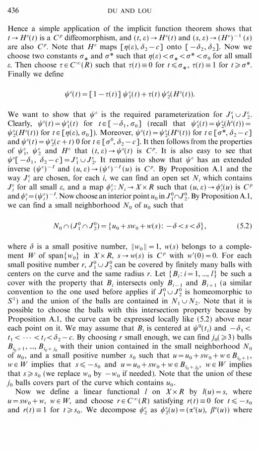
File: DISTL2 339447 . By:CV . Date:18:03:98 . Time:09:29 LOP8M. V8.B. Page 01:01Codes: 3646 Signs: 2513 . Length: 45 pic 0 pts, 190 mm
Hence a simple application of the implicit function theorem shows thatt � H=(t) is a C p diffeomorphism, and (t, =) � H=(t) and (s, =) � (H=)&1 (s)are also C p. Note that H = maps ['(=), $2&c] onto [&$2 , $2]. Now wechoose two constants _
*and _* such that '(=)<_
*<_*<_0 for all small
=. Then choose { # C�(R) such that {(t)#0 for t�_*
, {(t)#1 for t�_*.Finally we define
�=(t)=[1&{(t)] �=1(t)+{(t) �=
2(H=(t)).
We want to show that �= is the required parameterization for J =1 _ J =
2 .Clearly, �=(t)=�=
1(t) for t # [&$1 , _0] (recall that �=1(t)=�=
2(h=(t))=
�=2(H
=(t)) for t # ['(=), _0]). Moreover, �=(t)=�=2(H
=(t)) for t # [_*, $2&c]and �=(t)=�=
2(c+t) 0 for t # [_0, $2&c]. It then follows from the propertiesof �=
1, �=2 and H= that (t, =) � �=(t) is C p. It is also easy to see that
�=[&$1 , $2&c]=J =1 _ J =
2. It remains to show that �= has an extendedinverse (�=)&I and (u, =) � (�=)&I (u) is C p. By Proposition A.1 and theway J =
i are chosen, for each i, we can find an open set Ni which containsJ=
i for all small =, and a map ,=i : Ni � X_R such that (u, =) � ,=
i(u) is C p
and ,=i=(�=
i )&I. Now choose an interior point u0 in J 0
1&J 02 . By Proposition A.1,
we can find a small neighborhood N0 of u0 such that
N0 & (J 01 & J 0
2)=[u0+sw0+w(s) : &$<s<$], (5.2)
where $ is a small positive number, &w0 &=1, w(s) belongs to a comple-ment W of span[w0] in X_R, s � w(s) is C p with w$(0)=0. For eachsmall positive number r, J 0
1 _ J 02 can be covered by finitely many balls with
centers on the curve and the same radius r. Let [Bi : i=1, ..., l] be such acover with the property that Bi intersects only Bi&1 and Bi+1 (a similarconvention to the one used before applies if J 0
1 _ J 02 is homeomorphic to
S1) and the union of the balls are contained in N1 _ N2 . Note that it ispossible to choose the balls with this intersection property because byProposition A.1, the curve can be expressed locally like (5.2) above neareach point on it. We may assume that Bi is centered at �0(ti) and &$1<t1< } } } <tl<$2&c. By choosing r small enough, we can find j0(�3) ballsBi0+1 , ..., Bi0+ j0
with their union contained in the small neighborhood N0
of u0 , and a small positive number s0 such that u=u0+sw0+w # Bi0+1 ,w # W implies that s�&s0 and u=u0+sw0+w # Bi0+ j0
, w # W impliesthat s�s0 (we replace w0 by &w0 if needed). Note that the union of thesej0 balls covers part of the curve which contains u0 .
Now we define a linear functional l on X_R by l(u)=s, whereu=sw0+w, w # W, and choose r # C�(R) satisfying r(t)#0 for t�&s0
and r(t)#1 for t�s0 . We decompose ,=2 as ,=
2(u)=(:=(u), ;=(u)) where
436 DU AND LOU

File: DISTL2 339448 . By:CV . Date:18:03:98 . Time:09:29 LOP8M. V8.B. Page 01:01Codes: 3006 Signs: 1713 . Length: 45 pic 0 pts, 190 mm
:=(u) # E and ;=(u) # R and define ,� =2(u)=(:=(u), (H=)&1 (;=(u))). Finally
define ,= : � li=1Bi � X_R by
,=(u)=(1&r(l(u&u0)) ,=1(u)+r(l(u&u0)) ,� =
2(u) for u # .j0
j=1
Bi0+ j ;
,=(u)=,=1(u) for u # .
i0
i=1
Bi ;
,=(u)=,� =2(u) for u # .
l
i=i0+ j0+1
Bi .
By the continuity of �= we know that for all small =, J =1 _ J 2
= are containedin the union of the l balls. To check that (u, =) � ,=(u) is C p, by the inter-section property of the balls, we need only check that on Bi0
_ Bi0+1 andon Bi0+ j0
_ Bi0+ j0+1 . But it turns out that on the first two balls, ,= agreeswith ,=
1 and on the other two balls, it agrees with ,� =2. It is straightforward
to check that ,=(�=(t))=(0, t) for t in a small neighborhood of [&$1 ,$2&c]. This completes our proof of the Claim. K
Remark A.4. 1. In Proposition A.1, if F is analytic, then the localparameterizations are also analytic. However, we have only a C� globalparameterization in Proposition A.3 even if F is analytic.
2. The perturbation parameter = need not be a real number. It can bean element in a Banach space.
Next we consider the case where (H1) and the following two conditionsare assumed.
(H4): F(x(=), *, =)=0 for all (*, =) near (*0 , 0), where = � x(=) is C p
and x(0)=0.
(H5): dim Ker(Fx(0, *0 , 0))=codim Range(Fx(0, *0 , 0))=1, Ker(Fx
(0, *0 , 0))=[x0] and Fx*(0, *0 , 0) x0 � Range(Fx(0, *0 , 0)).
Then a simple variant of the proof of Theorem 1.7 in Crandall�Rabinowitz [8] shows the following result is valid.
Proposition A.5. Under the assumptions (H1), (H4) and (H5), there isa neighborhood U of (0, *0 , 0) and a positive number $ such that
F &1(0) & U=[(sx0+sz(s, =), *(s, =), =) : s, = # (&$, $)]
_ [(x(=), *, =) : (x(=), *, =) # U],
where z and * are C p&1 with z(0, 0)=0, *(0, 0)=*0 , z(s, =) belongs to acomplement Z of span[x0] in X.
437S-SHAPED GLOBAL BIFURCATION CURVE

File: DISTL2 339449 . By:CV . Date:18:03:98 . Time:09:29 LOP8M. V8.B. Page 01:01Codes: 3376 Signs: 1698 . Length: 45 pic 0 pts, 190 mm
Remark A.6. A similar result (but in a less general form) to Proposi-tion A.5 can be found in Chow and Hale [5], where they suppose thatu(=)#0 and Fx(0, *, =) does not depend on =.
There is also an easy generalization of Theorem 1.16 in Crandall�Rabinowitz [9] to the above case. Following the proof there, we have thefollowing result.
Proposition A.5$. Under the conditions and notations of PropositionA.5, there exist open intervals I, J with *0 # I, 0 # J and C p&1 functions# : I_J � R, + : J_J � R, u : I_J � X and w : J_J � X such that
Fx(x(=), *, =) u(*, =)=#(*, =) u(*, =) for * # I, = # J,
Fx(sx0+sz(s, =), *(s, =), =) w(s, =)=+(s, =) w(s, =) for s, = # J.
Moreover,
#(*0 , 0)=+(0, 0)=0, u(*0 , 0)=w(0, 0)=x0 ,
u(*, =)&x0 # Z, w(s, =)&x0 # Z,
and #*(*0 , 0){0
lims � 0, +(s, 0){0
&s*s(s, 0) #*(*0 , 0)+(s, 0)
=1.
ACKNOWLEDGMENTS
Part of this work was done while Y. Du was visiting Sydney University. The hospitality hereceived there is gratefully acknowledged. He would especially like to thank Prof. E. N.Dancer there for many interesting discussions. Y. Lou thanks K. Ball, E. Carlen, D. Jerison,and M. Loss for helpful discussions. The research of Y. Du was partially supported by a grantfrom the Australian Research Council, that of Y. Lou at MSRI was supported by NSF grantDMS No. 9022140.
We also wish to thank the anonymous referee for helpful comments.
REFERENCES
1. M. Berger and B. Gostiaux, ``Differential Geometry: Manifolds, Curves, and Surfaces,''Springer-Verlag, Berlin�New York, 1988.
2. K. J. Brown, Nontrivial solutions of predator-prey systems with small diffusion, NonlinearAnal. 11 (1987), 685�689.
3. J. Blat and K. J. Brown, Global bifurcation of positive solutions in some systems ofelliptic equations, SIAM J. Math. Anal. 17 (1986), 1339�1353.
438 DU AND LOU

File: DISTL2 339450 . By:CV . Date:18:03:98 . Time:09:29 LOP8M. V8.B. Page 01:01Codes: 9548 Signs: 3440 . Length: 45 pic 0 pts, 190 mm
4. A. Casal, J. C. Eilbeck, and J. Lopez-Gomez, Existence and uniqueness of coexistencestates for a predator-prey model with diffusion, Differential Integral Equations 7 (1994),411�439.
5. S. N. Chow and J. K. Hale, ``Methods of Bifurcation Theory,'' Springer-Verlag, Berlin�New York, 1982.
6. E. D. Conway, R. Gardner, and J. Smoller, Stability and bifurcation of steady-statesolutions for predator-prey equations, Adv. in Appl. Math. 3 (1982), 288�334.
7. M. G. Crandall and P. H. Rabinowitz, The Hopf bifurcation theorem in infinite dimen-sions, Arch. Rational Mech. Anal. 67 (1977), 53�72.
8. M. G. Crandall and P. H. Rabinowitz, Bifurcation from simple eigenvalues, J. Funct. Anal.8 (1971), 321�340.
9. M. G. Crandall and P. H. Rabinowitz, Bifurcation, perturbation of simple eigenvalues andlinearized stability, Arch. Rational Mech. Anal. 52 (1973), 161�180.
10. E. N. Dancer, On the structure of solutions of an equation in catalysis theory when aparameter is large, J. Differential Equations 37 (1980), 404�437.
11. E. N. Dancer, On the indices of fixed points of mappings in cones and applications,J. Math. Anal. Appl. 91 (1983), 131�151.
12. E. N. Dancer, On positive solutions of some pairs of differential equations, Trans. Amer.Math. Soc. 284 (1984), 729�743.
13. E. N. Dancer, On positive solutions of some pairs of differential equations, II, J. Differen-tial Equations 60 (1985), 236�258.
14. E. N. Dancer, Counterexamples to some conjectures on the number of solutions ofnonlinear equations, Math. Ann. 272 (1985), 421�440.
15. E. N. Dancer, On uniqueness and stability for solutions of singularly perturbatedpredator-prey type equations with diffusion, J. Differential Equations 102(1) (1993),1�32.
16. E. N. Dancer, Multiple fixed points of positive maps, J. Reine Angew. Math. 371 (1986),46�66.
17. E. N. Dancer and Y. Du, Competing species equations with diffusion, large interactionsand jumping nonlinearities, J. Differential Equations 114 (1994), 434�475.
18. Y. Du, Uniqueness, multiplicity and stability for positive solutions of a pair of reaction�diffusion equations, Proc. Roy. Soc. Edinburgh Section A 126 (1996), 777�809.
19. Y. Du and Y. Lou, Some uniqueness and exact multiplicity results for a predator-preymodel, Trans. Amer. Math. Soc. 349 (1997), 2443�2475.
20. B. D. Hassard, N. D. Kazarinoff and Y.-H. Wan, ``Theory and Applications of HopfBifurcation,'' Cambridge Univ. Press, Cambridge, UK, 1981.
21. D. Henry, ``Geometric Theory of Semilinear Parabolic Equations,'' Lecture Notes inMathematics, Vol. 840, Springer-Verlag, Berlin�New York, 1981.
22. T. Kato, ``Perturbation Theory for Linear Operators,'' Springer-Verlag, Berlin�New York,1966.
23. P. Korman and A. W. Leung, A general monotone scheme for elliptic system with applica-tions to ecological models, Proc. Roy. Soc. Edinburgh Section A 102 (1986), 315�325.
24. N. Lakos, Existence of steady-state solution for one-predator, two-prey system, SIAM J.Math. Anal. 21 (1990), 647�659.
25. L. Li, Coexistence theorems of steady-states for predator-prey interacting systems, Trans.Amer. Math. Soc. 305 (1988), 143�166.
26. L. Li, On the uniqueness and ordering of steady-states of predator-prey systems, Proc.Roy. Soc. Edinbutgh Section A 110 (1989), 295�303.
27. J. Lopez-Gomez and R. Pardo, Existence and uniqueness of coexistence states for thepredator-prey model with diffusion: the scalar case, Differential Integral Equations 6(5)(1993), 1025�1031.
439S-SHAPED GLOBAL BIFURCATION CURVE

File: 505J 339451 . By:CV . Date:18:03:98 . Time:13:16 LOP8M. V8.B. Page 01:01Codes: 1742 Signs: 496 . Length: 45 pic 0 pts, 190 mm
28. C. V. Pao, On nonlinear reaction-diffusion systems, J. Math. Anal. Appl. 87 (1982),165�198.
29. C. V. Pao, ``Nonlinear Parabolic and Elliptic Equations,'' Plenum, New York, 1992.30. Y. Yamada, Stability of steady-states for prey-predator diffusion equations with
homogeneous Dirichlet conditions, SIAM J. Math. Anal. 21 (1990), 327�345.31. Q. X. Ye and Z. Y. Li, ``Introduction to Reaction-Diffusion Equations,'' Science Press,
Beijing, P. R. China, 1990. [in Chinese]
� � � � � � � � � �
440 DU AND LOU


