Dynamics of the Kirchho� Equations I: CoincidentCenters of Gravity and BuoyancyPhilip Holmes1;2, Je�rey Jenkins1, and Naomi Ehrich Leonard11 Department of Mechanical and Aerospace Engineering,Princeton University, Princeton, NJ 08544, U.S.A.2 Program in Applied and Computational Mathematics,Princeton University, Princeton, NJ 08544, U.S.A.August 6, 1997AbstractWe study the Kirchho� equations for a rigid body immersed inan incompressible, irrotational, inviscid uid in the case that the cen-ters of buoyancy and gravity coincide. The resulting dynamical equa-tions form a non-canonical Hamiltonian system with a six-dimensionalphase space, which may be reduced to a four-dimensional (two-degree-of-freedom, canonical) system using the two Casimir invariants of mo-tion. Restricting ourselves to ellipsoidal bodies, we identify severalcompletely integrable sub-cases. In the general case, we analyse ex-istence, linear and nonlinear stability, and bifurcations of equilibriacorresponding to steady translations and rotations, including mixedmodes involving simultaneous motion along two body axes, some ofwhich we show can be stable. By perturbing from the axisymmetric,integrable case, we show that slightly asymmetric ellipsoids are typi-cally non-integrable, and we investigate their dynamics with a view tousing motions along homo- and heteroclinic orbits to execute speci�cmaneuvers in autonomous underwater vehicles.1 Introduction: the Kirchho� equationsKirchho�'s equations provide a model of a rigid body submerged in an ideal uid. Under circumstances in which viscous e�ects are small, it is common to1

use these equations to describe the dominant dynamics of an underwater ve-hicle. One is particularly interested in having such a low-dimensional modelin order to design control laws for underwater vehicles that are unmannedand must manage their own motion. For such autonomous underwater ve-hicles (AUVs), it is a priority to design control laws that are e�cient, sincepower is limited to what can be carried on board.In this light, we study the dynamics of Kirchho�'s equations as part ofan e�ort to exploit underwater vehicle dynamics to advantage in the designof motion control laws. For example, we expect to be able to use the resultsof our investigation to accomplish maneuvers that make use of the naturalglobal nonlinear dynamics and, as a result, require reduced external controle�ort. In particular, we expect to use homoclinic and heteroclinic orbitsand other phase space structures resulting from symmetries of Kirchho�'sequations to suggest stabilization and control strategies much as Bloch andMarsden [1] and Coller et al. [2, 3] did earlier for models of the boundarylayer.Kirchho�'s equations are derived under the assumption that the rigidbody is submerged in an in�nitely large volume of irrotational, incompress-ible, inviscid uid that is at rest at in�nity. De�ne v and ! to be the linearand angular velocity vectors, respectively, for the rigid body expressed withrespect to a frame �xed on the body with origin at the center of buoyancy.Let p and � be the linear and angular momentum vectors, respectively, alsowith respect to the body-�xed frame. We note that these latter vectors aremore correctly identi�ed as impulse since they include only the �nite partof the momentum of the body- uid system, but for convenience we will re-fer to them as momentum vectors. The relationship between velocity andmomentum is given by �p ! = I DDT M ! !v ! 4= M !v ! ;where M is a symmetric positive de�nite matrix. Here, I is the sum ofthe body inertia matrix plus the added inertia matrix associated with thepotential ow model of the uid. Similarly, M is the sum of the mass matrixfor the body alone, i.e., the mass of the body m0 multiplied by the identitymatrix, plus the added mass matrix associated with the uid. D accounts forcoupling terms. The body axes can always be chosen so thatM is diagonal,i.e., one chooses them to be the principal axes of the added mass ellipsoid.Kirchho�'s equations for the dynamics of the submerged body are then2

given by _� = � � ! + p� v + T_p = p � ! + F ; (1)where T and F are external torques and forces, respectively. We assume thatthe only external forces and torques are those due to gravity and buoyancy.For practical purposes, we consider a neutrally buoyant vehicle, i.e., a vehiclewith gravitational force equal and opposite to buoyant force. In this case,there are no external forces and T = �m0g� � rG where g is gravitationalacceleration, rG is the vector from the center of buoyancy to the center ofgravity and � is the unit vector pointing in the direction of gravity andexpressed with respect to the body-�xed frame. � evolves according to_� = � � ! :In this paper, as a �rst step, we consider only the case in which the centerof buoyancy and the center of gravity coincide (i.e., the mass of the bodyis uniformly distributed). In this case, Kirchho�'s equations are given by(1) with T = F = 0 and they can be viewed as Lie-Poisson (non-canonicalHamiltonian) dynamics on se(3)�, the dual of the Lie algebra of the group ofrigid body motions, SE(3), with � = (�;p) an element in se(3)� [4]. Thus,the equations are equivalent to _�i = f�i; Hg, where the Poisson bracket onse(3)� is de�ned by fG;Kg(�) = rG ��(�)rKfor di�erentiable functions G;K on se(3)�. Here�(�) = � pp 0 ! ;and the operator ^maps vectors in IR3 to the 3�3 skew-symmetric matricesas �y = � � y for y 2 IR3. The Hamiltonian H is simply the total kineticenergy of the body- uid systemH(�) = 12� � M�1� :Two independent Casimir functions, Ci : se(3)� ! IR areC1 = p � � ; C2 = jpj2 :3

These functions Poisson commute with any functionK on se(3)�, i.e., fCi; Kg =0, and thus are conserved quantities along the equations of motion.The Lie-Poisson dynamics on se(3)� can be interpreted as resulting fromreduction by the symmetry group SE(3) of the \full" dynamics on thetwelve-dimensional phase space T �SE(3). Here, symmetry means that theHamiltonian that describes the dynamics in T �SE(3) is invariant to actionsof SE(3), i.e., one can translate the inertial frame or rotate it in any direc-tion without a�ecting the equations of motion. A pair (R;b) 2 SE(3) =SO(3) � IR3 describes the orientation and position of the vehicle with re-spect to inertial coordinates. The evolution ofR and b can be reconstructed,given the solution to the Lie-Poisson equations, according to_R = R!_b = Rv : (2)For simplicity in stating explicit parametric criteria, we will further spe-cialize in this paper to the case of an ellipsoidal vehicle. Choosing the axesof the body-�xed frame to coincide with the principal axes of the ellipsoid,this yields M = 0B@ m1 0 00 m2 00 0 m3 1CA ; I = 0B@ I1 0 00 I2 00 0 I3 1CA ;and D = 0. As described above, each mass and inertia term is the sum ofa component due to the body and a component due to the uid. That dueto the uid is a function of the lengths of the semiaxes of the ellipsoid andthe uid density. De�ne li to be the length of the semiaxis of the ellipsoidalvehicle along the ith principal axis for i = 1; 2; 3: The volume of the ellipsoidis V = 4�l1l2l3=3. Then, letting � be the density of the uid and de�ningfor i = 1; 2; 3, i = l1l2l3 Z 10 d�(l2i + �)� ;� = q(l21 + �)(l22 + �)(l23 + �) ;the mass term mi is given bymi = m0 + �V i2� i= �V (1 + i2� i ) ; (3)4

where the second equality follows because the vehicle is taken to be neutrallybuoyant. Similarly,I1 = 15m0(l22 + l23) + 15�V (l22 � l23)2( 3 � 2)2(l22 � l23) + (l22 + l23)( 2 � 3)!= 15�V l22 + l23 + (l22 � l23)2( 3 � 2)2(l22 � l23) + (l22 + l23)( 2� 3)! : (4)See [5] for details of the derivation. The formulae for the inertia terms I2and I3 are cyclic permutations of the formula for I1 (1 7! 2 7! 3). We havewritten a short Mathematica code to calculate these expressions from thesemiaxis lengths. Via the i, these expressions involve incomplete ellipticintegrals.Throughout this paper, without loss of generality, we will take l1 > l2 �l3. This implies that the mass terms are always ordered as m3 � m2 > m1,while the inertia terms may be ordered as I3 � I2 > I1, as I2 � I3 > I1,or as I2 > I1 > I3, depending on the relative lengths of the li [6]. Inthe Appendix we provide a calculation which shows how the inertia termsare ordered for small perturbations from the symmetric case l2 = l3 (inwhich case I3 = I2 > I1 and m3 = m2 > m1). It reveals that a smalldecrease in the ratio l3=l2 will yield I3 > I2 > I1 when l1=l2 < c and willyield I2 > I3 > I1 when l1=l2 > c, where c � 1:62. This result is usefulfor perturbation calculations from the symmetric case that we do later inthe paper. For completeness, we explore the existence of relative equilibriaand the nature of stability of these relative equilibria for all three possibleorderings of inertia terms.Kirchho�'s equations are Hamiltonian when restricted to a level set(coadjoint orbit) C1 = p � �, C2 = jpj2. In the generic case in whichC2 6= 0, these level sets are di�eomorphic to TS2, the four-dimensional tan-gent bundle to the sphere [4] (an explicit coordinate system for this space,di�ering from that of [4], is given in Section 2). If on these level sets, there isa conserved quantity in addition to the Hamiltonian, then the equations areintegrable. In general, the Kirchho� equations are nonintegrable, as shownin the paper of Kozlov and Onishchenko [7], although only the special case ofa system close to pure spin, for which jpj � 1, is explicitly considered in thatpaper. Aref and Jones [8] performed numerical simulations and showed howsome of the resulting chaotic motions correspond to irregular tumbling ofthe vehicle. There are, however, several special integrable cases, which havebeen described by Kirchho�, Clebsch, Steklov, Liouville and others and are5

catalogued, for example, in the paper of Rubanovskii [9]. We discuss theseintegrable cases further in Section 2 as they are useful as limits to perturbfrom in our global analysis.Stability of equilibria of Kirchho�'s equations was studied in [6, 10].In [6], the centers of buoyancy and gravity for the submerged rigid bodywere not assumed to be coincident, introducing the additional torque T =�m0g� � rG, as described above, into Kirchho�'s equations. The Lie-Poisson structure was derived for the corresponding equations, and Lya-punov stability was studied for several examples of equilibria using theenergy-Casimir method. As a special case, Lyapunov stability was stud-ied for an ellipsoidal body with coincident centers and an axis of symmetry.These stability analyses were extended in [10]. In particular, a methodis given for determining directions of drift in the original phase space cor-responding to stable equilibria in the reduced space for mechanical sys-tems with non-compact symmetry groups (such as SE(3) in the presentcase). Typically, there will be no drift in the directions corresponding tothe compact part of the symmetry group, but drift in some if not all of thenon-compact symmetry directions. Novikov and Shmel'tser [4] comment onthe possibility of such drift. The stability techniques of [10] also includethe means, under certain conditions, for determining stability of nongenericequilibria, i.e., equilibria that do not live on a coadjoint orbit of maximalrank (such as the rising and spinning, bottom-heavy, submerged rigid body).The paper is organized as follows. In Section 2 we describe invariantsubspaces and integrability cases, and introduce an explicit canonical coor-dinate system. In Section 3 we describe families of equilibria, their linearized(spectral) stability, and local bifurcations. Nonlinear (Lyapunov) stabilityof these equilibria is discussed in Section 4, resulting in an almost completecharacterization of stability types. A partial analysis of global behavior,focussing on homoclinic orbits, is presented in Section 5, where we extendthe results of [7] by considering the fate of homoclinic manifolds of solu-tions, possessed by axisymmetric bodies, under perturbation to small non-axisymmetry. Not only do we prove nonintegrability in this case, but we alsoinvestigate the consequences of the perturbed homoclinic and heteroclinicorbits for motions of an AUV in physical space in Section 6, thus extendingthe work of [8]. We summarise in Section 7. Computational details areprovided in the Appendix. 6

2 Invariant subspaces and integrable limitsIn this section we collect a number of more or less well-known results onKirchho�'s equations which we shall use subsequently.Henceforth we specialise to the case of an ellipsoidal body with coincidentcenters of buoyancy and gravity, for which the Hamiltonian is simply thetotal kinetic energy in body coordinates:H(p;�) = 12 3Xi=1 �2iIi + 12 3Xi=1 p2imi : (5)Equations (1) then take the form, in components:_p1 = 1I3 p2�3 � 1I2 p3�2_p2 = 1I1 p3�1 � 1I3 p1�3_p3 = 1I2 p1�2 � 1I1 p2�1_�1 = � 1I3 � 1I2� �2�3 + � 1m3 � 1m2� p2p3_�2 = � 1I1 � 1I3� �3�1 + � 1m1 � 1m3� p3p1_�3 = � 1I2 � 1I1� �1�2 + � 1m2 � 1m1� p1p2 : (6)The Casimir invariants are: C1 = p � � = ab ; (7)and C2 = jpj2 = a2 ; (8)the constants a � 0; b will be used below. Note that their existence impliesthat the six-dimensional phase space of (6) is foliated by a two-parameterfamily of invariant four-dimensional leaves Ma;b.The vector �eld de�ned by Equation (6) is equivariant under the follow-ing symmetries:(p1; p2; p3; �1; �2; �3; t) 7! (�p1;�p2; p3;��1;��2; �3; t) 7!(p1; p2;�p3; �1; �2;��3;�t) ; (9)7

and the cyclic permutations thereof. Thus it is a reversible dynamical sys-tem [11] and the hyperplanes pj = �j = 0 are symmetric sections, in theteminology of [12]. We will use these symmetries in the global analysis ofSection 5.Equations (6) have several invariant subspaces that will be useful inglobal analysis.2.1 Pure spinIt is clear that the subspace S = fp = 0 (a = 0)g is invariant for (6). On Sthe dynamics is just that of the classical free rigid body [13, 14]. Here theresticted kinetic energy TS and the magnitude of body angular momentumare constants of motion:TS = 12 3Xi=1 �2iIi ; j�j2 = 3Xi=1 �2i ; (10)so, as is well-known, this subsystem is completely integrable. Its solutionslie on the intersections of energy ellipsoids and momentum spheres given by(10).2.2 Planar MotionsSimilarly, the subspace F1 = f�2 = �3 = p1 = 0g, and its two cyclicpermutations F2;F3, are invariant. On F1 the system reduces to:_p2 = 1I1 p3�1_p3 = � 1I1 p2�1_�1 = � 1m3 � 1m2� p2p3 ; (11)with constants of motion:TF = 12 �21I1 + p22m2 + p23m3! ; C2;F = p22 + p23 = a2 ; (12)so that this subsystem is also completely integrable, with solutions lying onthe intersections of ellipsoids and cylinders given by (12). (Note that theother Casimir C1;F � 0 on each Fj .) 8

2.3 Axisymmetric body: the Lagrange caseIf two of the mass and inertia elements coincide, Equations (6) are also com-pletely integrable in a manner analogous to the Lagrange case of the heavytop [13]. Supposing that m2 = m3 and I2 = I3, it is clear that �1 remainsconstant, and so provides an additional integral. To reveal the global struc-ture of solutions, however, the following coordinate change, originally dueto Deprit, is useful (cf. [15]):0B@ �1�2�3 1CA = 0B@ s~r cos�~r sin � 1CA ; (13)0B@ p1p2p3 1CA = ar2 264b0B@ s~r cos �~r sin � 1CA + �r0B@ �~rs cos �s sin � 1CA cos�+ �r0B@ 0�r sin �r cos � 1CA sin �375 ;(14)where ~r = +pr2 � s2 and �r = +pr2 � b2.It is easy to check that this transformation automatically ensures preser-vation of the Casimir invariants (7-8), so that it provides an explicit pa-rameterisation of the four-dimensional manifold Ma;b. Moreover, as shownin [15], the new variables (r; s; �; �) are canonical on each Ma;b. Indeed,substituting (13-14) for � and p in (5), we obtain the explicit two-degree-of-freedom system:_r = @H@� ; _� = �@H@r ; _s = @H@� ; _� = �@H@s : (15)Note that, when jpj = a = 0, the variable � disappears from H and ishence cyclic, so that r is conserved. When m2 = m3 = m and I2 = I3 = I ,H simpli�es to:H0(r; s; �) =12 "a2� 1m1 � 1m��bs� ~r�r cos�r2 �2 + r2I + � 1I1 � 1I� s2 + a2m# ;(16)in this case � is a cyclic variable and s = �1 is conserved. We will usethis limiting case below in Section 2.5 and subsequently in perturbationcalculations in Section 5. 9

Novikov and Shmel'tser [4] de�ne a related set of non-canonical coordi-nates on Ma;b, for which the reduced Hamiltonian equations analogous to(15) contain an additional \magnetic" term.2.4 The Clebsch case: invariant planesThere are other, less well-known, completely integrable cases, as describedin [16], for example.1 Consider the quadratic function�1(p1; �2; �3) = p21 + k I1I3�22I1 � I3 + I1I2�23I1 � I2! (17)and its cyclic permutations (1 7! 2 7! 3), �2(p2; �3; �1) and �3(p3; �1; �2). Itis easy to check that all three �j are constants of motions for (6) providedthat the following equality holds, along with its cyclic permutations:�1 = 1I1 + kI2I3(m3 �m2)m2m3(I3 � I2) = 0 : (18)Here k in (17) may be chosen freely. These conditions can be satis�ed formj , Ij all distinct if the single relation among the mj and Ij holds:m1I1(m3 �m2) +m2I2(m1 �m3) +m3I3(m2 �m1) = 0 : (19)Note that this may be achieved by the choice1mj = � + �IjI1I2I3 ; (20)for arbitrary �; �. Under this assumption, any one of the �j provides anindependent integral in addition to C1, C2 and H , so that the system iscompletely integrable in the classical sense of [13]. Other sub-cases aredetailed in [16].We note an apparently unremarked geometric consequence of (19): thisequality implies the existence of a family of invariant subspaces of the formpj = �j�j : (21)Indeed, as detailed in the Appendix, substituting (21) into (6) we obtainthree equations for the �j which admit nontrivial solutions if and only if a1We learned of these from R. Camassa and D. Holm, who kindly shared with us theirunpublished work on the Kirchho� and C. Neumann tops.10

certain 3� 3 determinant vanishes. This occurs precisely when (19) holds.Eliminating pj via (21), on the invariant subspace (6) reduces to a systemanalogous to the free rigid body:_�1 = 1�1 ��2I3 � �3I2��2�3_�2 = 1�2 ��3I1 � �1I3��3�1_�3 = 1�3 ��1I2 � �2I1��1�2 ; (22)the ow of which preserves the functions3Xi=1 �i�2i = ab and 3Xi=1 �2i �2i = a2 ; (23)which are just the Casimirs (7-8) in this special case.2.5 A reduced, canonical representationIn Subsection 2.3 above we displayed a canonical coordinate system in whichthe integrable structure of certain special cases becomes transparent. Thesecoordinates are also useful in cases for which additional integrals do notexist, and they may be used to prove non-integrability and the presence ofchaotic solutions in some such cases. Here we display the Hamiltonian andequations of motion for the general non-axisymmetric case.We will be particularly interested in perturbing from the case m2 =m3 = m; I2 = I3 = I . In view of this it is convenient to make the followingde�nitions: m2 = m; m3 = m1� �m ; I2 = I; I3 = I1 + �I ; (24)in which case substitution of (13-14) into (5) yieldsH = H0(r; s; �)+H�(r; s; �; �) ; (25)with H0 given as in (16) andH� = 12 (��ma2m �b~r sin � + �r(s sin � cos �+ r cos� sin �)r2 �2+ �II (r2 � s2) sin2 �� : (26)11

The resulting canonical equations of motion take the form:_r = AB � �r~r sin �r2 �� �mC � �r(�s sin � sin �+ r cos� cos �)r2 �_� = AB "2bsr3 + �r2s2 + ~r2b2r3�r~r ! cos�#� rI � �II r sin2 �+�mC "b�r(2s2 � r2) sin� + ~rs(2b2 � r2) sin � cos�+ b2r~r cos� sin �)r3�r~r #_s = �II (r2 � s2) sin � cos� � �mC �b~r cos � + �r(s cos� cos�� r sin � sin �)r2 �_� = �AB �b+ (s�r=~r) cos�r2 �� � 1I1 � 1I� s+ �II s sin2 �+�mC ��(bs=~r) sin� + �r sin � cos�r2 � ; (27)where A = a2� 1m1 � 1m� ; B = B(r; s; �) = bs� �r~r cos�r2 ; and (28)C = C(r; s; �; �) = a2m �b~r sin � + �r(s sin� cos�+ r cos � sin �)r2 � :Note that these equations are exact (the asymmetry parameters �m and �Ido not need to be small), but that the transformation (13-14) is singularat r = s and r = b. Also, observe that the \leading" terms in (27) (thoselacking the factors �I and �m) are the explicit expressions of Equations (15)in the axisymmetric case; indeed, for �I = �m = 0 _s � 0, as claimed (� is acyclic variable). We will use this coordinate system in Section 5.3 Steady motions, equilibria and linearised sta-bilityIn this section we describe families of equilibria and study their linearisedstability. Also, for the symmetric integrable case of Section 2.3, we displaya family of periodic solutions.3.1 Pure and mixed mode equilibriaTo �nd equilibrium solutions it is convenient to write (6) in the form:_p = p� ! ; _� = � � ! + p� v ; (29)12

cf. (1). Thus, for equilibria we require p0 � !0 = 0 or !0 = �p0, for some� 2 IR. Substituting this into �0�!0+p0�v0 = 0 and using the de�nitionsof p =Mv and � = I!, we �nd the conditions: � � 1mj + �2Ij! p0j = 0 ; j = 1; 2; 3 ; �0j = �Ijp0j ; (30)where � 2 IR also. Equations (30) clearly admit three (classical) branchesof pure mode �xed points of the forms(p;�) = (p01; 0; 0; �01; 0; 0) (31)= (0; p02; 0; 0; �02; 0) (32)= (0; 0; p03; 0; 0; �03) ; (33)for arbitrary p0j ; �0j , regardless of the mass and inertia values mj ; Ij (simplyset � = 1m1 � �2I1, with arbitrary � and p2 = p3 = 0, for example). Thesewe call, naturally enough, the pure 1, 2 and 3 modes. Each pure modecorresponds to steady translation in the direction of a principle axis, withspin about that axis, and it belongs to a two-parameter family that is mostconveniently characterised by the ratio of angular to linear momentum,�0jp0j = p � �jpj2 = ba ; (34)the magnitude of which we henceforth denote by jb=aj = .When I3 > I2 > I1, the pure modes are the only equilibria possible, butfor certain other orderings of mass and inertia values, mixed mode branchescan also be found. As described in Section 1, we �x m3 � m2 > m1. Then,in addition to the case I3 > I2 > I1 and depending on the choice of ellip-soid axes, both of the following orderings of inertias can occur, as well asthe coincident cases separating them. Under these conditions we have, forarbitrary p02; p03:I2 > I3 > I1 : Mixed 2{3 mode:�23 = s m3 �m2m2m3(I2 � I3) ; �23 = m2I2 �m3I3m2m3(I2 � I3) ;�0j = ��23Ijp0j ; j = 2; 3 ; �1 = p1 = 0 : (35)13

I2 > I1 > I3 : Mixed 2{3 mode as above, and mixed 1-3 mode:�13 = s m3 �m1m1m3(I1 � I3) ; �13 = m1I1 �m3I3m1m3(I1 � I3) ;�0j = ��13Ijp0j ; j = 1; 3 ; �2 = p2 = 0 : (36)These solutions exist only for limited ranges of the angular momentumto linear momentum ratio de�ned in (34). Speci�cally, (35) exists for�23I3 < = j p �� jjpj2 = ���� ba ���� < �23I2 ; (37)and (36) for �13I3 < = j p �� jjpj2 = ���� ba ���� < �13I1 : (38)At the ends of these ranges the mixed modes coalesce with the pure 3 and2, and 3 and 1 modes respectively. Note that, if I2 > I1 > I3, we necessarilyhave �23 < �13; this implies that the bifurcation points on the pure 3 branchare always ordered in the same way; see Equations (48-49), below.These mixed mode solutions do not appear to have been recognised orstudied previously. They correspond to translation along an axis in the 2{3or 1{3 plane respectively (as de�ned by the body axes), combined with spinabout a di�erent axis in the same plane.3.2 Linearised stabilityElementary (if tedious) linearisation of Equation (6) at the pure and mixedmode equilibria yields a set of eigenvalue problems having characteristicpolynomials of the form: �2(�4 + 2c2�2 + c0) = 0 : (39)The double zero eigenvalue is mandated by the structure of the problem;it corresponds to eigenvectors in the directions transverse to the invariantsurfaces de�ned by the Casimirs (7-8); the remaining eigenvalues are gen-erally non-zero and form a quartet in the complex plane, as in canonical14

Hamiltonian systems. The coe�cients c0 and c2 take the following forms:Pure 1 mode:c0 = � 1I2I3 24(I1 � I2) �01I1 !2 + �m1 �m2m1m2 � (p01)235 �24(I3 � I1) �01I1 !2 + �m3 �m1m3m1 � (p01)235 ;2c2 = 24�1� (I1 � I2)(I3 � I1)I2I3 � �01I1 !2+ �m1 �m2m1m2I3 + m1 �m3m1m3I2 � (p01)2� : (40)Analogous expressions for the pure 2 and 3 modes are obtained by cyclicpermutation of the mass and inertia terms. For the mixed modes (35) and(36) we have:Mixed 2{3 mode:c0 = 4�m3 �m2m2m3 ���m3 �m2m2m3 ��I3 � I1I1I2I3 �+ �m3 �m1m1m3 ��I2 � I3I1I2I3 �� (p02p03)2 ; (41)2c2 = "�m3 �m2m2m3 � (I2 � I3)2 + I1(2I3 � I2)I1I3(I2 � I3) !+ m2 �m1m1m2I3 # (p02)2+ "�m3 �m2m2m3 � (I2 � I3)2 + I1(2I2 � I3)I1I2(I2 � I3) !+ m3 �m1m1m3I2 # (p03)2 :Mixed 1-3 mode:c0 = 4�m1 �m3m3m1 ���m1 �m3m3m1 ��I1 � I2I1I2I3 �+ �m1 �m2m2m1 ��I3 � I1I1I2I3 �� (p03p01)2 ; (42)2c2 = "�m1 �m3m1m3 � (I3 � I1)2 + I2(2I1 � I3)I2I1(I3 � I1) !+ m3 �m2m2m3I1 # (p03)215

+ "�m1 �m3m1m3 � (I3 � I1)2 + I2(2I3 � I1)I2I3(I3 � I1) !+ m1 �m2m2m1I3 # (p01)2 :Using these formulae and the appropriate ordering of mass and inertiaelements, we may solve for the non-trivial eigenvalues from (39),� = �r�c2 �qc22 � c0 ; (43)and deduce the following linearised stability results, which we state in termsof the momentum ratio de�ned in (34):I3 > I2 > I1 : Mode 1 is unstable for < 1H and linearly stable for > 1H , where 21H = I2I3F1I2 + I3 � I1 241 +s1� �F2F1�235 ; (44)and F1 = �m2 �m1m1m2 ��2I3 � I1I3 �+ �m3 �m1m1m3 ��2I2 � I1I2 � ;F2 = �m2 �m1m1m2 ��I1I3�� �m3 �m1m1m3 ��I1I2� : (45)At 1H a Hamiltonian Hopf bifurcation occurs. We note that when m2 =m3 = m; I2 = I3 = I , (44-45) reduces to the simple expression: 21H = 4(m�m1)Imm1 : (46)Mode 2 is unstable for all , and mode 3 is linearly stable for all .I2 > I3 > I1 : Mode 1 is unstable for < 1H and linearly stable for > 1H , with 1H de�ned as above. Mode 2 is unstable for < 2P andlinearly stable for > 2P , where 2P = �23I2 = s m3 �m2m2m3(I2 � I3) I2 : (47)16

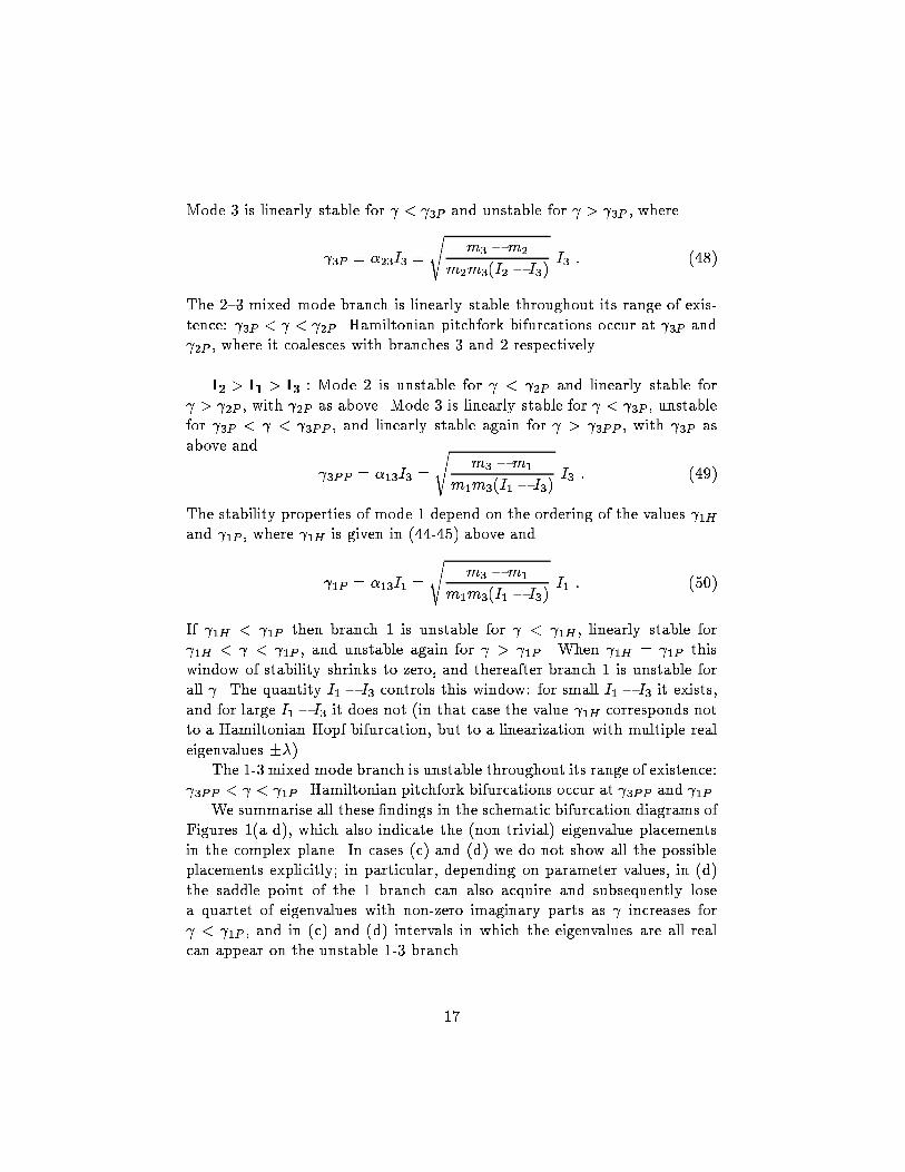
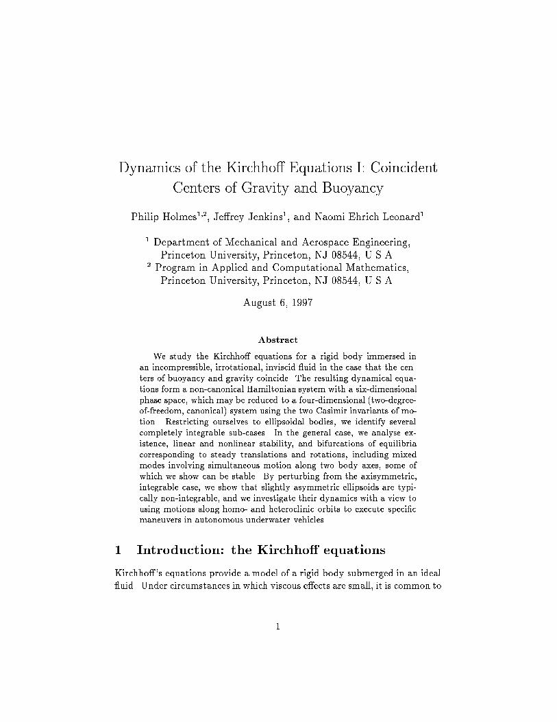
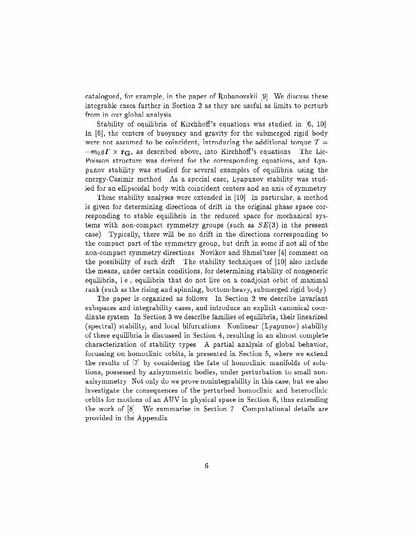
Mode 3 is linearly stable for < 3P and unstable for > 3P , where 3P = �23I3 = s m3 �m2m2m3(I2 � I3) I3 : (48)The 2{3 mixed mode branch is linearly stable throughout its range of exis-tence: 3P < < 2P . Hamiltonian pitchfork bifurcations occur at 3P and 2P , where it coalesces with branches 3 and 2 respectively.I2 > I1 > I3 : Mode 2 is unstable for < 2P and linearly stable for > 2P , with 2P as above. Mode 3 is linearly stable for < 3P , unstablefor 3P < < 3PP , and linearly stable again for > 3PP , with 3P asabove and 3PP = �13I3 = s m3 �m1m1m3(I1 � I3) I3 : (49)The stability properties of mode 1 depend on the ordering of the values 1Hand 1P , where 1H is given in (44-45) above and 1P = �13I1 = s m3 �m1m1m3(I1 � I3) I1 : (50)If 1H < 1P then branch 1 is unstable for < 1H , linearly stable for 1H < < 1P , and unstable again for > 1P . When 1H = 1P thiswindow of stability shrinks to zero, and thereafter branch 1 is unstable forall . The quantity I1 � I3 controls this window: for small I1 � I3 it exists,and for large I1� I3 it does not (in that case the value 1H corresponds notto a Hamiltonian Hopf bifurcation, but to a linearization with multiple realeigenvalues ��).The 1-3 mixed mode branch is unstable throughout its range of existence: 3PP < < 1P . Hamiltonian pitchfork bifurcations occur at 3PP and 1P .We summarise all these �ndings in the schematic bifurcation diagrams ofFigures 1(a-d), which also indicate the (non-trivial) eigenvalue placementsin the complex plane. In cases (c) and (d) we do not show all the possibleplacements explicitly; in particular, depending on parameter values, in (d)the saddle point of the 1 branch can also acquire and subsequently losea quartet of eigenvalues with non-zero imaginary parts as increases for < 1P , and in (c) and (d) intervals in which the eigenvalues are all realcan appear on the unstable 1-3 branch.17

1

2

30

1H

(a)

1

2

30

1H

(b)

2P

3P

1

2

30

1H

(c)

2P

3P 3PP

1P

1

2

30

(d)

2P

3P 3PP

1PFigure 1: Equilibrium solutions corresponding to pure and mixedtranslation-spin motions. (a) I3 > I2 > I1; (b) I2 > I3 > I1; (c)I2 > I1 > I3, small I1 � I3; (d) I2 > I1 > I3, large I1 � I3. Solid linesindicate linearly stable equilibria; dotted, chain dotted, and dashed linesindicate unstable equilibria with eigenvalue placements as shown in insetsand described in text. Boldened solid portions indicate nonlinearly stableequilibria, as described in Section 4.18

3.3 Some special periodic solutionsIn the axisymmetric case m2 = m3 = m; I2 = I3 = I a family of periodicorbits can be found as follows. One seeks solutions of the form(p1; p2; p3; �1; �2; �3) =(p01; c cos(!t); c sin(!t); �01; d cos(!t); d sin(!t)) ;substitutes into (6), and solves the resulting linear equations for p01 and �01in terms of the amplitudes c; d and frequency !: p01�01 ! = �!D cdI� 1m1 � 1m� c2 + d2I ! ; (51)where D = � 1I1 � 1m1 � 1m� c2 + 1I � 1I1 � 1I�d2� > 0 : (52)This yields a three-parameter (c; d; !) family of \circular" periodic orbitswithC1 = p � � = ab = p01�01 + cd ; and C2 = jpj2 = a2 = (p01)2 + c2 ; (53)and with momentum ratio given by:p � �jpj2 = ba = dnD2 + !2 h1I � 1m1 � 1m� c2 + d2I2 iocnD2 + !2 d2I2o : (54)Thus, on a constant a; b level set, we have a one-parameter family of periodicmotions.Various other explicit solutions can be found in this integrable case,including the homoclinic orbits to the (unstable) pure 1 mode discussed inSection 5.1.4 Nonlinear stability of pure and mixed modesIn this section we study nonlinear (Lyapunov) stability of the families ofequilibria described in Section 3. We use the energy-Casimir method whichgives a procedure to construct a Lyapunov function to prove nonlinear sta-bility for an equilibrium of a Lie-Poisson system.19

For a generic equilibrium �e of a Lie-Poisson system, the Lyapunov func-tion is constructed from the Hamiltonian, the Casimir functions, and anyother conserved quantities. Speci�cally, we set H�;� = H + �(Ci) + �j(cj),where H is the Hamiltonian, Ci are the Casimirs, cj are other constantsof motion and �(�) and �j(�) are smooth functions to be determined in thecourse of the analysis. We �rst choose �(�) and �j(�) such that �e is acritical point of H�;�. The additional condition that the second variationof H�;� (the matrix of second partial derivatives) be positive or negativede�nite at �e is then su�cient for nonlinear stability of �e, since near �ethe level sets of H�;� form codimension-one hypersurfaces homeomorphic tonested spheres, to which solutions remain con�ned. For further details see[17, 18].We assume that p 6= 0, so that the equilibria are all generic (p = 0gives the pure spin case of Section 2.1). We begin by studying the nonlinearstability of the pure mode equilibria. Consider the conserved quantityH�(�) = H(�) + �(C1(�); C2(�))= 12(p �M�1p+ � � I�1�) + �(p � �; 12 jpj2) ;where �(C1; C2) is to be determined (for ease of computation C2 as de�nedin (8) has here been multiplied by 1/2). In practice it is su�cient to take aquadratic polynomial in C1; C2, the coe�cients of which are determined bythe �rst and second derivative conditions noted above.We �rst treat the family of equilibria corresponding to the pure 1 modedescribed by (31), i.e.,�e = (p;�) = (p01; 0; 0; �01; 0; 0) :A straightforward computation analogous to that in [6], and sketched in theAppendix, shows that, evaluated at this equilibrium, H� can be chosen withits �rst derivative zero and second derivative (positive) de�nite if and onlyif for both i = 2 and i = 3� 1Ii � 1I1� 1I1 �01p01 !2 > 1Ii � 1m1 � 1mi� : (55)This is therefore a su�cient condition for nonlinear stability of the 1 mode.Similarly (using the permutation symmetry of (6)), we �nd that the pure2 mode is nonlinearly stable if for both i = 1 and i = 3� 1Ii � 1I2� 1I2 �02p02!2 > 1Ii � 1m2 � 1mi� ; (56)20

and the pure 3 mode is nonlinearly stable if for both i = 1 and i = 2� 1Ii � 1I3� 1I3 �03p03 !2 > 1Ii � 1m3 � 1mi� : (57)These conditions can be interpreted for the various admissible orderingsof inertia terms. Recall the de�nition of from Section 3: = jp ��jjpj2 ;which for the pure j mode becomes simply = ������0jp0j ����� :I3 > I2 > I1 : The su�cient condition for nonlinear stability fails forboth mode 1 and mode 2. Mode 3 is nonlinearly stable for all (wherep03 6= 0).I2 > I3 > I1 : The su�cient condition for stability fails for mode 1.Mode 2 is nonlinearly stable if = ������02p02 ����� > s m3 �m2m2m3(I2 � I3)I2 = 2P : (58)Note that, excluding the case of equality, this is also a necessary condition fornonlinear stability of mode 2 (see the linear stability analysis of Section 3.2,Equation (47)). Mode 3 is nonlinearly stable if = ������03p03 ����� < s m3 �m2m2m3(I2 � I3)I3 = 3P : (59)Excluding the case of equality, this too is a necessary condition for nonlinearstability of mode 3 (see Equation (48)).I2 > I1 > I3 : The su�cient condition for stability fails for mode 1.Mode 2 is nonlinearly stable if and only if = ������02p02 ����� > s m3 �m2m2m3(I2 � I3)I2 = 2P ; (60)where we have excluded the case of equality. Mode 3 is nonlinearly stable if = ������03p03 ����� < s m3 �m2m2m3(I2 � I3)I3 = 3P : (61)21

We cannot, however, conclude in this case that the condition is necessaryfor nonlinear stability of Mode 3.The stability of these pure modes was studied in [6, 10] for the specialcase of a body with an axis of symmetry coinciding with the axis of trans-lation. In this case there is an additional conserved quantity with whichthe function H� can be augmented. Under these circumstances mode 3 isalways nonlinearly stable and modes 1 and 2 are nonlinearly stable if andonly if is su�ciently high.Next we treat the family of equilibria corresponding to the 2{3 mixedmode described by (35), i.e.,�e = (p;�) = (0; p02; p03; 0;��23I2p02;��23I3p03) ;where �23 = s m3 �m2m2m3(I2 � I3) :In both cases of inertia ordering for which this mixed mode can occur, i.e.,I2 > I3 > I1 and I2 > I1 > I3, a computation similar to that for the puremode case, also sketched in the Appendix, shows that H� can be chosen sothat its �rst derivative, evaluated at this equilibrium, is zero and its secondderivative is (positive) de�nite as long as p02p03 6= 0. This implies that the2{3 mixed mode is nonlinearly stable throughout its range of existence forall p02p03 6= 0.We have already shown in Section 3.2 that the 1-3 mixed mode describedby (36) is linearly unstable for all cases in which it occurs (I2 > I1 > I3).The energy-Casimir method condition for nonlinear stability necessarily failsin this situation.Our nonlinear stability results are summarized in Figure 1, along withthe linearised stability results of Section 3. Comparing them, it is apparentthat some cases remain to be resolved, for which an equilibrium is linearlystable but the energy-Casimir method does not provide su�cient conditionsto conclude nonlinear stability. Failure of the method to demonstrate non-linear stability does not imply instability. In fact, numerical simulationsin these cases suggest stability, and since we have a two degree of freedomsystem, we can appeal to KAM theory [14, 19] to conclude the existenceof invariant tori supporting quasiperiodic ow which locally separate thereduced phase space near these branches of equilibria, implying that orbitsremain bounded. However, it has been shown that in such circumstances22

the equilibrium does become unstable with the addition of a certain type ofdissipation [20].These results allow one to conclude nonlinear stability of the given equi-libria in the six-dimensional reduced space se(3)�. This directly implies thatthe corresponding relative equilibrium ze in the full phase space T �SE(3) isstable modulo the symmetry group SE(3). This suggests that, although mo-mentum variables behave stably, rotation angles and position variables maydrift. However, application of the theory of [10] leads to a stronger conclu-sion with regard to which variables may drift. In particular, for each of thenonlinear stability conclusions above, the stronger version of the energy-Casimir method described in [10] implies that the corresponding relativeequilibrium ze is stable in T �SE(3) modulo SE(2)� IR. Thus, while posi-tion variables may drift, rotation variables cannot drift away from the axisof rotation.5 Global behavior, bifurcation and homoclinic or-bits5.1 Homoclinic orbits to the pure 1 modeIn this subsection we establish nonintegrability of (6) for the parameters �mand �I su�ciently small, i.e, for m2 � m3 and I2 � I3, and for all in abroad range below 1H, the point at which pure mode 1 loses stability in aHamiltonian Hopf bifurcation. We use the reduced, canonical representationof (27) and appeal to Melnikov's method [19] as adapted and generalised totwo-degree-of-freedom Hamiltonian systems in [21], cf. [15]. In those papersit is shown that, if the Melnikov integral evaluated along an unperturbedhomoclinic orbit to a hyperbolic periodic orbit:M(�0) = Z 1�1 �H0; H� � (r(t); �(t); s= b; �(t) + �0)dt ; (62)has simple zeroes as a function of �0, then for � 6= 0 su�ciently small,the perturbed system has transverse homoclinic orbits and hence Smalehorseshoes [19] in its dynamics. Here is given at leading order by_� = 0(r; �; s= b) = @H�@s (6= 0) : (63)23

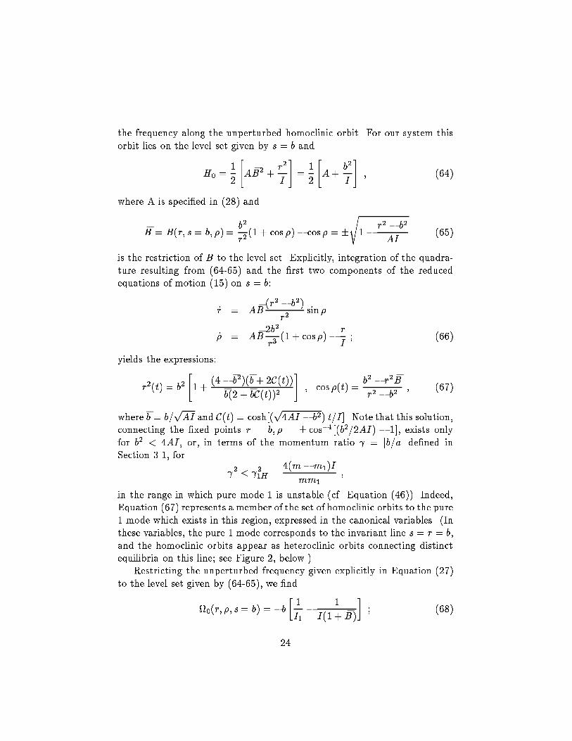
the frequency along the unperturbed homoclinic orbit. For our system thisorbit lies on the level set given by s = b andH0 = 12 "A �B2 + r2I # = 12 "A+ b2I # ; (64)where A is speci�ed in (28) and�B = B(r; s = b; �) = b2r2 (1 + cos �)� cos� = �s1� r2 � b2AI (65)is the restriction of B to the level set. Explicitly, integration of the quadra-ture resulting from (64-65) and the �rst two components of the reducedequations of motion (15) on s = b:_r = A �B (r2 � b2)r2 sin �_� = A �B 2b2r3 (1 + cos�)� rI ; (66)yields the expressions:r2(t) = b2 "1 + (4� �b2)(�b+ 2C(t))�b(2 + �bC(t))2 # ; cos �(t) = b2 � r2 �Br2 � b2 ; (67)where �b = b=pAI and C(t) = cosh[(p4AI � b2) t=I ]. Note that this solution,connecting the �xed points r = b; � = � cos�1[(b2=2AI) � 1], exists onlyfor b2 < 4AI , or, in terms of the momentum ratio = jb=aj de�ned inSection 3.1, for 2 < 21H = 4(m�m1)Imm1 ;in the range in which pure mode 1 is unstable (cf. Equation (46)). Indeed,Equation (67) represents a member of the set of homoclinic orbits to the pure1 mode which exists in this region, expressed in the canonical variables. (Inthese variables, the pure 1 mode corresponds to the invariant line s = r = b,and the homoclinic orbits appear as heteroclinic orbits connecting distinctequilibria on this line; see Figure 2, below.)Restricting the unperturbed frequency given explicitly in Equation (27)to the level set given by (64-65), we �nd0(r; �; s= b) = �b � 1I1 � 1I(1 + �B)� ; (68)24

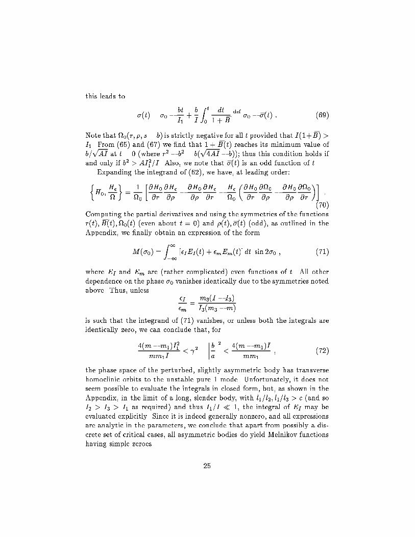
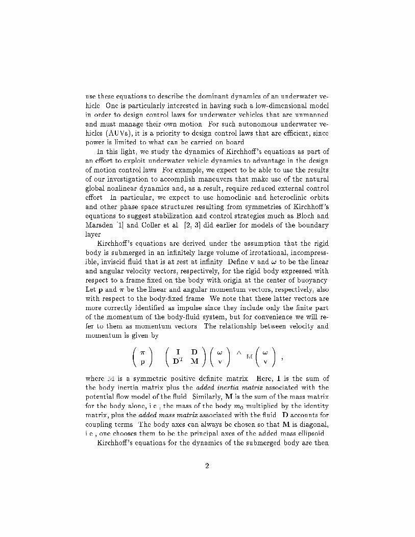
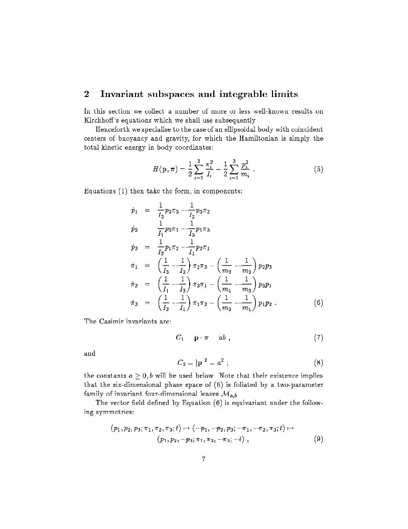
this leads to �(t) = �0 � btI1 + bI Z t0 dt1 + �B def= �0 � ��(t) : (69)Note that 0(r; �; s= b) is strictly negative for all t provided that I(1+ �B) >I1. From (65) and (67) we �nd that 1 + �B(t) reaches its minimum value ofb=pAI at t = 0 (where r2 � b2 = b(p4AI � b)); thus this condition holds ifand only if b2 > AI21=I . Also, we note that ��(t) is an odd function of t.Expanding the integrand of (62), we have, at leading order:�H0; H� � = 10 �@H0@r @H�@� � @H0@� @H�@r � H�0 �@H0@r @0@� � @H0@� @0@r �� :(70)Computing the partial derivatives and using the symmetries of the functionsr(t); �B(t);0(t) (even about t = 0) and �(t); ��(t) (odd), as outlined in theAppendix, we �nally obtain an expression of the formM(�0) = Z 1�1 [�IEI(t) + �mEm(t)]dt sin 2�0 ; (71)where EI and Em are (rather complicated) even functions of t. All otherdependence on the phase �0 vanishes identically due to the symmetries notedabove. Thus, unless �I�m = m3(I � I3)I3(m3 �m)is such that the integrand of (71) vanishes, or unless both the integrals areidentically zero, we can conclude that, for4(m�m1)I21mm1I < 2 = ���� ba ����2 < 4(m�m1)Imm1 ; (72)the phase space of the perturbed, slightly asymmetric body has transversehomoclinic orbits to the unstable pure 1 mode. Unfortunately, it does notseem possible to evaluate the integrals in closed form, but, as shown in theAppendix, in the limit of a long, slender body, with l1=l2; l1=l3 > c (and soI2 > I3 > I1 as required) and thus I1=I � 1, the integral of EI may beevaluated explicitly. Since it is indeed generally nonzero, and all expressionsare analytic in the parameters, we conclude that apart from possibly a dis-crete set of critical cases, all asymmetric bodies do yield Melnikov functionshaving simple zeroes. 25

��������������������������������������������������������������������������������������������������������������������������������������������������������������������������������������������������������������������������������������������������������������������������������������������������������������������������������������������������������������������������������������������������������������������������������������������������������������������������������������������������������������������

Figure 2: Homoclinic orbits to the pure 1 mode in the canonical coordinates(r; �), with I1 = 1; I = 2;m1 = 1; m = 2. (a) The integrable system:�m = �I = 0; (b) The perturbed system: �m = �I = 0:2. Several solutionsare shown, starting with di�erent initial phases �0, illustrating the e�ect oftransverse homoclinic orbits.Figure 2 illustrates the e�ect of symmetry breaking and the resultingtransverse homoclinic orbits, showing that orbits can now pass to either sideof the saddle point(s), depending upon initial phase. The resulting orbitsare, however, only mildly chaotic in the original p;� coordinates, since theyall follow approximately the same routes in phase space, and only di�er insubtle details of their behavior near the equilibrium.We note that in [22], by analysis of the normal form, it is shown that�nite sets of homoclinic solutions to the unstable solution exist in the neigh-borhood of a Hamiltonian Hopf bifurcation point for any reversible system.5.2 Homoclinic and heteroclinic orbits to the pure 2 and 3modesFor the case I2 > I3, in the parameter range 3P < < 2P , the puremodes 2 and 3 are both unstable and of saddle-center type, and they coexistwith the stable 2{3 mixed mode. Numerical integrations of Equation (6)suggest that homoclinic or near-homoclinic orbits to these pure modes mayexist in this range. Since on any orbit, the total energy H (Equation (5))is conserved as well as the Casimirs C1 and C2 (Equations (7)-(8)), thereduced phase space is three-dimensional. Generically, with one-dimensionalstable and unstable manifolds in a three-dimensional ow, intersections arecodimension two phenomena which we expect only at isolated points in atwo-parameter family of systems; however, the symmetries (9) imply that for26

this reversible system, such homo- or heteroclinic connections are genericallycodimension one phenomena [12, 23]. Thus we may expect connections tooccur for isolated values of the momentum ratio = jb=aj.We can easily �nd necessary conditions for such connections. We �xC2 = a2 = 1 without loss of generality and use the fact that the pure 2and 3 modes generally lie on di�erent energy levels for given , except at = �23pI2I3, the geometric mean of 3P and 2P , where all these equilibrialie on the same level set. Only here are heteroclinic connections among all2 and 3 modes possible, otherwise we expect at most orbits connecting2 or 3 modes to themselves. More speci�cally, for just above 3P , anormal form computation shows that homoclinic loops from the equilibrium(0; 0; p03; 0; 0; �03) to itself are likely, while loops from (0; p02; 0; 0; �02; 0) to itselfare likely for just below 2P . For < �23pI2I3, the 2 modes provide anenergy barrier preventing orbits leaving the positive (resp. negative) 3 modesfrom crossing \to the other side", thus p3(t) and �3(t) must retain the samesigns. Similar observations apply to p2(t) and �2(t) for orbits asymptotic tothe 2 modes for > �23pI2I3.Unfortunately, we cannot carry out a direct perturbation study of thesehomoclinic orbits as in Section 5.1 for homoclinic orbits to the pure 1 mode.In the symmetric limiting case, the distinct pure 2 and 3 modes and themixed 2{3 mode all coalesce in a circle of degenerate equilibria, each of whichhas two zero eigenvalues in addition to the two zero eigenvalues enforced bythe constants of motion C1 and C2. (To see this, let m2 = m3 and I2 = I3 inthe appropriate cyclic permutations of Equation (40) and in Equation (41),and note that c0 = 0 in all cases. More trivially, from Equation (6) withm2 = m3 and I2 = I3, any solution of the form (0; p02; p03; 0; �02; �03) is a �xedpoint provided p02=p03 = �02=�03; enforcing the constraints (7-8) yields thecircle of equilibria.)We may get an indication of how this degenerate invariant set breaksup in the asymmetric system by appeal to the averaging theorem [14, 19].Assuming that the angular variable � is rapidly varying ( _�� 1), we averageEquations (27) with respect to �, using the operation�f = limT!1 1T Z T0 f(r; �; s; �) d� ;in which the remaining variables r; s; � are held constant. This is most easilydone by averaging the Hamiltonians H0 and H� of (16) and (26). Since �has been removed by this procedure, the resulting Hamiltonian system hasthe conjugate variable r as a constant of motion, and so may be integrated27

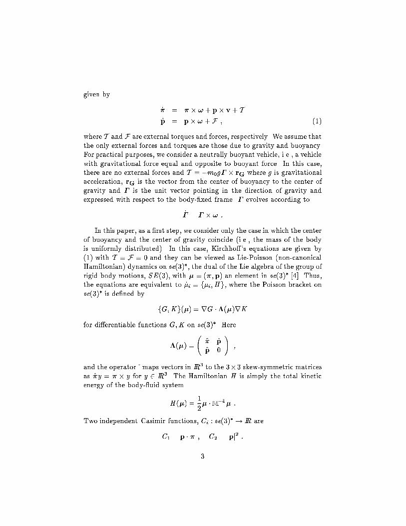
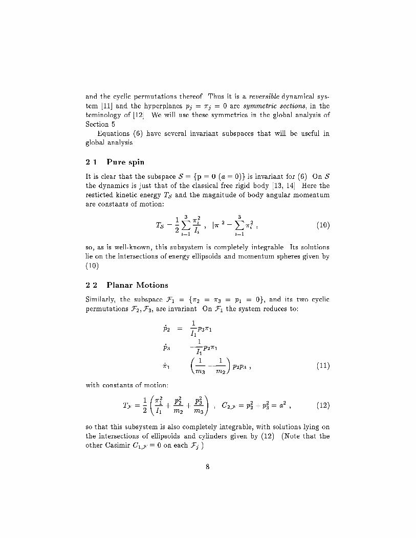
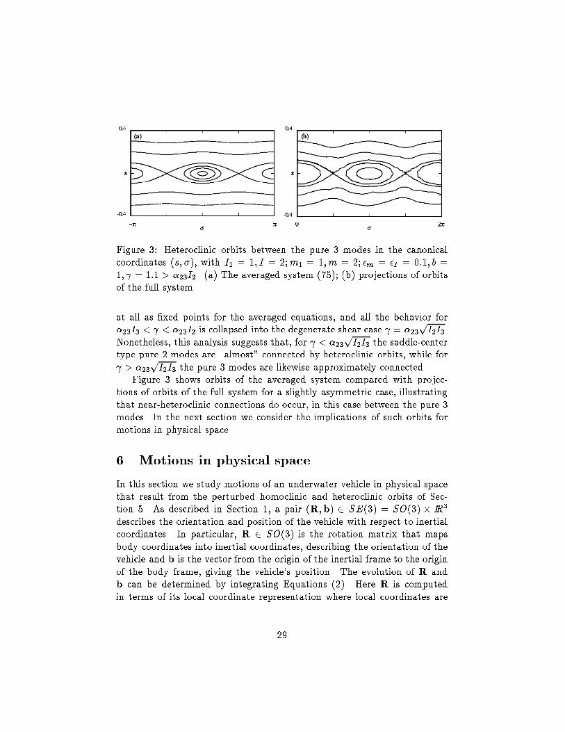
even when �I ; �m 6= 0. The reduced Hamiltonian equations in (s; �) are:_s = �II � �ma2m �D(r; b)!(r2 � s2) sin� cos �_� = � �a2 � 1m1 � 1m� �D(r; b) + � 1I1 � 1I�� s+ �II � �ma2m �D(r; b)!s sin2 � ; (73)where �D(r; b) = 3b2 � r22r4 : (74)We are interested in solutions lying in the level sets containing eitherthe pure 2 or pure 3 modes (0;�a; 0; 0;�b; 0); (0; 0;�a; 0; 0;�b). Via thetransformation (13-14), these are given by � = 0; � and � = �=2; 3�=2respectively, with s = 0 and r = b. In this case we have �D(r; b) = 1=b2 andEquations (73) reduce to:_s = ��II � �m 2m� (b2 � s2) sin � cos�_� = � � 1 2 � 1m1 � 1m�+ � 1I1 � 1I�� s+��II � �m 2m� s sin2 � : (75)These equations are easily analysed (they are essentially equivalent to thesimple pendulum), and we �nd that, when �I ; �m > 0 (the case I2 > I3 >I1), the 2 and 3 mode equilibria are respectively saddles and centers for < �23pI2I3, and respectively centers and saddles for > �23pI2I3. Notethat, for the symmetric system �I = �m = 0 and when = �23pI2I3,the ow of (75) reduces to linear shear about the circle s = 0 of �xedpoints. For �m > 0 > �I (the case I3 > I2 > I1), the 2 and 3 modeequilibria are respectively saddles and centers for all . In all cases thesaddles of (75) are connected by heteroclinic orbits. This reduced systemtherefore captures the leading order stability behavior of the pure modes,as per Sections 3.2 and 4, but it fails to reproduce the detailed behaviorincluding the mixed 2{3 mode in the case I2 > I3 > I1, involving lossof stability of mode 3 at = �23I3 < �23pI2I3, and gain of stability ofmode 2 at = �23I2 > �23pI2I3; indeed, the mixed modes do not appear28

��������������������������������������������������������������������������������������������������������������������������������������������������������������������������������������������������������������������������������������������������������������������������������������������������������������������������������������������������������������������������������������������������������������������������������������������������������������������������������������������������������������������

Figure 3: Heteroclinic orbits between the pure 3 modes in the canonicalcoordinates (s; �), with I1 = 1; I = 2;m1 = 1; m = 2; �m = �I = 0:1; b =1; = 1:1 > �23I2. (a) The averaged system (75); (b) projections of orbitsof the full system.at all as �xed points for the averaged equations, and all the behavior for�23I3 < < �23I2 is collapsed into the degenerate shear case = �23pI2I3.Nonetheless, this analysis suggests that, for < �23pI2I3 the saddle-centertype pure 2 modes are \almost" connected by heteroclinic orbits, while for > �23pI2I3 the pure 3 modes are likewise approximately connected.Figure 3 shows orbits of the averaged system compared with projec-tions of orbits of the full system for a slightly asymmetric case, illustratingthat near-heteroclinic connections do occur, in this case between the pure 3modes. In the next section we consider the implications of such orbits formotions in physical space.6 Motions in physical spaceIn this section we study motions of an underwater vehicle in physical spacethat result from the perturbed homoclinic and heteroclinic orbits of Sec-tion 5. As described in Section 1, a pair (R;b) 2 SE(3) = SO(3) � IR3describes the orientation and position of the vehicle with respect to inertialcoordinates. In particular, R 2 SO(3) is the rotation matrix that mapsbody coordinates into inertial coordinates, describing the orientation of thevehicle and b is the vector from the origin of the inertial frame to the originof the body frame, giving the vehicle's position. The evolution of R andb can be determined by integrating Equations (2). Here R is computedin terms of its local coordinate representation where local coordinates are29

0 500 1000 15000

200

400

600

t

γ 1

0 500 1000 1500−2

0

2

t

γ 2

0 500 1000 1500−2

0

2

t

γ 3

0 500 1000 15000

5

10

15

t

b 1

0 500 1000 1500−0.2

0

0.2

t

b 2

0 500 1000 1500

0

t

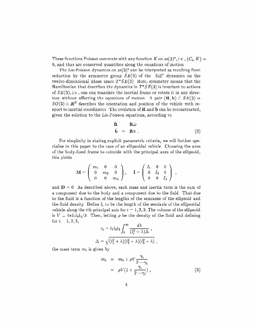
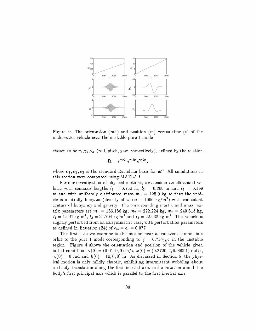
b 3Figure 4: The orientation (rad) and position (m) versus time (s) of theunderwater vehicle near the unstable pure 1 mode.chosen to be 1, 2, 3, (roll, pitch, yaw, respectively), de�ned by the relationR = e 1e1e 2e2e 3e3 ;where e1; e2; e3 is the standard Euclidean basis for IR3. All simulations inthis section were computed using MATLAB.For our investigation of physical motions, we consider an ellipsoidal ve-hicle with semiaxis lengths l1 = 0:750 m, l2 = 0:200 m and l3 = 0:199m and with uniformly distributed mass m0 = 125:0 kg so that the vehi-cle is neutrally buoyant (density of water is 1000 kg/m3) with coincidentcenters of buoyancy and gravity. The corresponding inertia and mass ma-trix parameters are m1 = 136:186 kg, m2 = 222:224 kg, m3 = 240:813 kg,I1 = 1:991 kg-m2, I2 = 24:704 kg-m2 and I3 = 22:938 kg-m2. This vehicle isslightly perturbed from an axisymmetric case, with perturbation parametersas de�ned in Equation (24) of �m = �I = 0:077.The �rst case we examine is the motion near a transverse homoclinicorbit to the pure 1 mode corresponding to = 0:75 1H: in the unstableregion. Figure 4 shows the orientation and position of the vehicle giveninitial conditions v(0) = (0:01; 0; 0) m/s, !(0) = (0:2720; 0; 0:00001) rad/s, i(0) = 0 rad and b(0) = (0; 0; 0) m. As discussed in Section 5, the phys-ical motion is only mildly chaotic, exhibiting intermittent wobbling abouta steady translation along the �rst inertial axis and a rotation about thebody's �rst principal axis which is parallel to the �rst inertial axis.30

0 10 20 30 40−2

0

2

t

γ 1

0 10 20 30 40−2

0

2

t

γ 2

0 10 20 30 400

50

100

150

t

γ 3

0 10 20 30 40−0.02

0

0.02

t

b 1

0 10 20 30 40−0.02

0

0.02

t

b 2

0 10 20 30 400

20

40

60

t

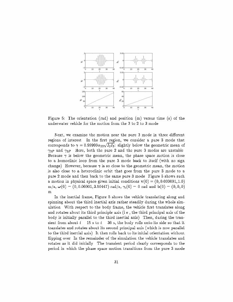
b 3Figure 5: The orientation (rad) and position (m) versus time (s) of theunderwater vehicle for the motion from the 3 to 2 to 3 mode.Next, we examine the motion near the pure 3 mode in three di�erentregions of interest. In the �rst region, we consider a pure 3 mode thatcorresponds to = 0:99999�23pI2I3: slightly below the geometric mean of 3P and 2P . Here, both the pure 2 and the pure 3 modes are unstable.Because is below the geometric mean, the phase space motion is closeto a homoclinic loop from the pure 3 mode back to itself (with no signchange). However, because is so close to the geometric mean, the motionis also close to a heteroclinic orbit that goes from the pure 3 mode to apure 2 mode and then back to the same pure 3 mode. Figure 5 shows sucha motion in physical space given initial conditions v(0) = (0; 0:000001; 1:0)m/s, !(0) = (0; 0:00001; 3:50447) rad/s, i(0) = 0 rad and b(0) = (0; 0; 0)m. In the inertial frame, Figure 5 shows the vehicle translating along andspinning about the third inertial axis rather steadily during the whole sim-ulation. With respect to the body frame, the vehicle �rst translates alongand rotates about its third principle axis (i.e., the third principal axis of thebody is initially parallel to the third inertial axis). Then, during the tran-sient from about t = 15 s to t = 30 s, the body rolls onto its side so that ittranslates and rotates about its second principal axis (which is now parallelto the third inertial axis). It then rolls back to its initial orientation without ipping over. In the remainder of the simulation the vehicle translates androtates as it did initially. The transient period clearly corresponds to theperiod in which the phase space motion transitions from the pure 3 mode31

0 10 20 30 40−5

0

5

t

γ 1

0 10 20 30 40−2

0

2

t

γ 2

0 10 20 30 400

50

100

t

γ 3

0 10 20 30 40−0.02

0

0.02

t

b 1

0 10 20 30 40−0.02

0

0.02

t

b 2

0 10 20 30 400

20

40

60

t

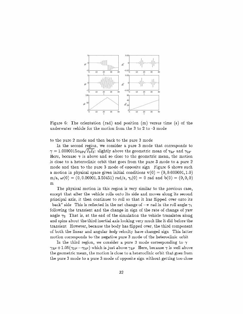
b 3Figure 6: The orientation (rad) and position (m) versus time (s) of theunderwater vehicle for the motion from the 3 to 2 to -3 mode.to the pure 2 mode and then back to the pure 3 mode.In the second region, we consider a pure 3 mode that corresponds to = 1:0000015�23pI2I3: slightly above the geometric mean of 3P and 2P .Here, because is above and so close to the geometric mean, the motionis close to a heteroclinic orbit that goes from the pure 3 mode to a pure 2mode and then to the pure 3 mode of opposite sign. Figure 6 shows sucha motion in physical space given initial conditions v(0) = (0; 0:000001; 1:0)m/s, !(0) = (0; 0:00001; 3:50451) rad/s, i(0) = 0 rad and b(0) = (0; 0; 0)m. The physical motion in this region is very similar to the previous case,except that after the vehicle rolls onto its side and moves along its secondprincipal axis, it then continues to roll so that it has ipped over onto its\back" side. This is re ected in the net change of �� rad in the roll angle 1following the transient and the change in sign of the rate of change of yawangle 3. That is, at the end of the simulation the vehicle translates alongand spins about the third inertial axis looking very much like it did before thetransient. However, because the body has ipped over, the third componentof both the linear and angular body velocity have changed sign. This lattermotion corresponds to the negative pure 3 mode of the heteroclinic orbit.In the third region, we consider a pure 3 mode corresponding to = 3P +1:05( 2P � 3P ) which is just above 2P . Here, because is well abovethe geometric mean, the motion is close to a heteroclinic orbit that goes fromthe pure 3 mode to a pure 3 mode of opposite sign without getting too close32

0 10 20 30 40−5

0

5

10

t

γ 1

0 10 20 30 40−2

0

2

t

γ 2

0 10 20 30 400

20

40

60

t

γ 3

0 10 20 30 40−0.02

0

0.02

t

b 1

0 10 20 30 40−0.02

0

0.02

t

b 2

0 10 20 30 400

20

40

60

t

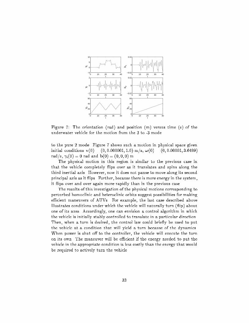
b 3Figure 7: The orientation (rad) and position (m) versus time (s) of theunderwater vehicle for the motion from the 3 to -3 mode.to the pure 2 mode. Figure 7 shows such a motion in physical space giveninitial conditions v(0) = (0; 0:000001; 1:0) m/s, !(0) = (0; 0:00001; 3:6499)rad/s, i(0) = 0 rad and b(0) = (0; 0; 0) m.The physical motion in this region is similar to the previous case inthat the vehicle completely ips over as it translates and spins along thethird inertial axis. However, now it does not pause to move along its secondprincipal axis as it ips. Further, because there is more energy in the system,it ips over and over again more rapidly than in the previous case.The results of this investigation of the physical motions corresponding toperturbed homoclinic and heteroclinic orbits suggest possibilities for makinge�cient maneuvers of AUVs. For example, the last case described aboveillustrates conditions under which the vehicle will naturally turn ( ip) aboutone of its axes. Accordingly, one can envision a control algorithm in whichthe vehicle is initially stably controlled to translate in a particular direction.Then, when a turn is desired, the control law could brie y be used to putthe vehicle at a condition that will yield a turn because of the dynamics.When power is shut o� to the controller, the vehicle will execute the turnon its own. The maneuver will be e�cient if the energy needed to put thevehicle in the appropriate condition is less costly than the energy that wouldbe required to actively turn the vehicle.33

7 ConclusionsIn this paper we have studied the dynamics of Kircho�'s equations describ-ing a submerged body with coincident centers of buoyancy and gravity. Thissix degree-of-freedom Hamiltonian system reduces to six �rst order di�er-ential equations on the phase space of linear and angular momentum inbody coordinates, and further, to a two-degree-of-freedom system when thetwo Casimir functions (invariants arising from the symmetry group of rigidmotions) are �xed. We describe an explicit canonical coordinate systemfor this reduction, and review some of the (extensive) literature on inte-grable cases. We then describe all the physically relevant equilibria (steadymotions) and determine their linearised stability, and, in most cases, theirnonlinear stability types. This includes mixed modes which do not appearto have been studied previously. We provide a partial analysis of homoclinicand heteroclinic motions in phase space that connect some of these equi-libria when they are unstable, and we use Melnikov's method to show thatslightly asymmetric bodies are chaotic in the sense that their reduced phasespaces contain Smale horseshoes. Finally, we reconstruct the physical spacemotions corresponding to some of these connecting and near-connecting or-bits, and suggest that they might provide mechanisms for low cost controlledmaneuvers of AUVs.AcknowledgementsThis work was supported by DoE Grant DE-FG02-95ER25238 (PH, JJ),by the National Science Foundation under Grant BES-9502477, and by theO�ce of Naval Research under Grant N00014-96-1-0052 (NEL, JJ).References[1] A.M. Bloch and J.E. Marsden. Controlling homoclinic orbits. Theoret-ical and Computational Fluid Dynamics, 1:179{90, 1989.[2] B.D. Coller, P. Holmes, and J.L. Lumley. Control of noisy heterocliniccycles. Physica D, 72:135{60, 1994.[3] B.D. Coller and P. Holmes. Suppression of bursting. Automatica, 33:1{11, 1997. 34

[4] S.P. Novikov and I. Shmel'tser. Periodic solutions of Kirchho�'s equa-tions for the free motion of a rigid body in a uid and the extendedtheory of Lyusternik-Shnirel'man-Morse (LSM). I. Funct. Anal. Appl.,15:197{207, 1982.[5] H. Lamb. Hydrodynamics. Cambridge University Press, Cambridge,UK, 1932. Sixth edition, reissued by Dover Publications, Inc. 1945.[6] N. E. Leonard. Stability of a bottom-heavy underwater vehicle. Auto-matica, 33(3):331{46, 1997.[7] V.V. Kozlov and D.A. Onishchenko. Nonintegrability of Kirchho�'sequations. Soviet Math Dokl., 26:495{98, 1983.[8] H. Aref and S.W. Jones. Chaotic motion of a solid through ideal uid.Phys. Fluids A, 5:3026{28, 1993.[9] V.N. Rubanovskii. Quadratic integrals of the equations of motion of arigid body in a liquid. J. Appl. Math. Mech., 52:312{322, 1988.[10] N. E. Leonard and J. E. Marsden. Stability and drift of underwatervehicle dynamics: Mechanical systems with rigid motion symmetry.Physica D, 105:130{162, 1997.[11] R.L. Devaney. Reversible di�eomorphism and ows. Trans. Amer.Math. Soc., 218:89{113, 1976.[12] A.R. Champneys. Homoclinic orbits in reversible systems and theirapplications in mechanics, uids and optics. Physica D, pages xx{xx,1997. To appear in a special issue for the Warwick Symposium onReversible Symmetries in Dynamical Systems.[13] H. Goldstein. Classical Mechanics. Addison Wesley, Reading, MA,1980. Second edition.[14] V.I. Arnold. Mathematical Methods of Classical Mechanics. SpringerVerlag, New York, 1978.[15] A. Mielke and P. Holmes. Spatially complex equilibria of buckled rods.Arch. Rat. Mech. Anal., 101:319{48, 1988.[16] O.I. Bogoyavlenskii. Integrable Euler equations on Lie algebras arisingin problems of mathematical physics. Math. USSR Izvestiya, 25:207{57,1985. 35

[17] D.D. Holm, J.E. Marsden, T. Ratiu, and A. Weinstein. Nonlinear sta-bility of uid and plasma equilibria. Physics Reports, 123:1{116, 1985.[18] J.E.Marsden and T.S. Ratiu. Introduction to Mechanics and Symmetry.Springer-Verlag, New York, NY, 1994.[19] J. Guckenheimer and P. Holmes. Nonlinear Oscillations, DynamicalSystems, and Bifurcations of Vector Fields. Springer-Verlag, New York,NY, 1990.[20] A. M. Bloch, P. S. Krishnaprasad, J. E. Marsden, and T. S. Ratiu.Dissipation induced instabilities. Ann. Inst. Henri Poincar�e, 11(1):37{90, 1994.[21] P. Holmes and J.E. Marsden. Horseshoes and Arnold di�usion forHamiltonian systems on lie groups. Indiana U. Math. J., 32:273{310,1983.[22] G. Iooss and M.C. P�erou�eme. Perturbed homoclinic solutions in re-versible 1:1 resonance vector �elds. J. Di�erential Equations, 102:62{88, 1993.[23] A. Mielke, P. Holmes, and O. O'Reilly. Cascades of homoclinic orbitsto, and chaos near, a Hamiltonian saddle-center. J. of Dynamics andDi�erential Equations, 4:95{126, 1992.Appendix: Computational detailsInertia orderings after perturbation from axisymmetric caseTo consider nearly-axisymmetric vehicles, it is necessary to determine theordering of inertia terms after perturbation. Without loss of generality,we will perturb from the case where the 2 and 3 axes are equal, that isl2 = l3; m2 = m3 and I2 = I3. Using the notation from Section 1, we have:I2 = 15�V l23 + l21 + (l23 � l21)2( 1 � 3)2(l23 � l21) + (l23 + l21)( 3� 1)!= 15�V 2(l43 � l41) + 4l21l23( 3 � 1)2(l23 � l21) + (l23 + l21)( 3 � 1)! ;36

I3 = 15�V l21 + l22 + (l21 � l22)2( 2 � 1)2(l21 � l22) + (l21 + l22)( 1� 2)!= 15�V 2(l41 � l42) + 4l21l22( 1 � 2)2(l21 � l22) + (l21 + l22)( 1 � 2)! :To determine the inertia ordering as the lengths l3 and l2 change rela-tive to one another, we consider the ratio l3=l2. In all cases we expect asmall perturbation to have no e�ect on the ordering of the I1 term, whichwill remain the smallest of the inertias (recall that throughout we assumel1 > l2 � l3). However, we expect a nearly spherical vehicle, with all axesrelatively similar in length, to adopt the perturbed inertia ordering of asphere, I3 > I2 > I1, while a cigar-shaped vehicle with l1 >> l2; l3 shouldhave the perturbed inertia ordering I2 > I3 > I1. Thus, it is likely that theratio l1=l2 will also be important. For this reason, we de�ne the parametersp = l1=l2 (> 0) and q = l3=l2 (> 0). For the perturbation calculation, we willconsider changes in q with p acting as a �xed parameter. The expressionsabove become:I2 = l225 �V 2(q4 � p4) + 4p2q2( 3 � 1)2(q2 � p2) + (q2 + p2)( 3� 1)! ;I3 = l225 �V 2(p4 � 1) + 4p2( 1 � 2)2(p2 � 1) + (p2 + 1)( 1 � 2)! ;where 1 � 2 and 3 � 1 are now: 1 � 2 = pq Z 10 (1� p2)(1 + t)(p2 + t)p(p2 + t)(q2 + t)(1 + t) dtdef= pq(1� p2)N2(p; q) ; 3 � 1 = pq Z 10 (p2 � q2)(q2 + t)(p2 + t)p(p2 + t)(q2 + t)(1 + t) dtdef= pq(p2 � q2)N3(p; q) :In order to determine the inertia ordering in the case of a nearly axisym-metric vehicle, it is su�cient to determine the rate of change with respectto q of the ratio I2=I3 when q = 1. To do this, we compute the values of N2,N3, @N2=@q, and @N3=@q at q = 1: 37

�N = N2 jq=1= N3 jq=1= Z 10 dt(1 + t)2(p2 + t)3=2 ;@ �N@q = @N2@q jq=1= 13 @N3@q jq=1= � Z 10 dt(1 + t)3(p2 + t)3=2 :Evaluating the integrals, we �nd:�N = p2 + 2p(p2 � 1)2 + 32(p2 � 1)5=2 log p�pp2 � 1p+pp2 � 1! ;@ �N@q = 12(p2 � 1) �52 �N � 1p� :After some calculations, we obtain an expression for the derivative of theinertia ratio at q = 1:@@q �I2I3� jq=1= 4� 8p3 �N + 2p(p2 � 1)2@ �N=@q + 4p6 �N22(p2 + 1)� 4p3 �N � p(p2 + 1)2 �N + 2p4(p2 + 1) �N2 : (76)In Figure 8 we display this function. Observe that the derivative changessign at p � 1:62, leading to the conclusions noted in Section 1.Invariant subspaces in the Clebsch caseWe seek conditions under which there exists a linear invariant subspace ofthe form (21) pj = �j�j , with the constants �j to be determined from theparameters Ij ; mj in the course of the analysis. Substitution of this ansatzinto (6) yields the following three conditions:�1�2�3�m2 �m3m2m3 � = �I2(�1 � �2) + I3(�1 � �3)I2I3�1�2�3�m3 �m1m3m1 � = �I3(�2 � �3) + I1(�2 � �1)I3I1�1�2�3�m1 �m2m1m2 � = �I1(�3 � �1) + I2(�3 � �2)I1I2 : (77)Letting �12 = �1 � �2;�13 = �1 � �3 and � = �1�2�3, we may rewrite (77)as a linear system:264 �I2 I3 I2I3m2m3 (m3 �m2)I3 � I1 �I3 I3I1m3m1 (m1 �m3)I2 I1 � I3 I1I2m1m2 (m2 �m1) 3750B@ �12�13� 1CA = 0B@ 000 1CA (78)38

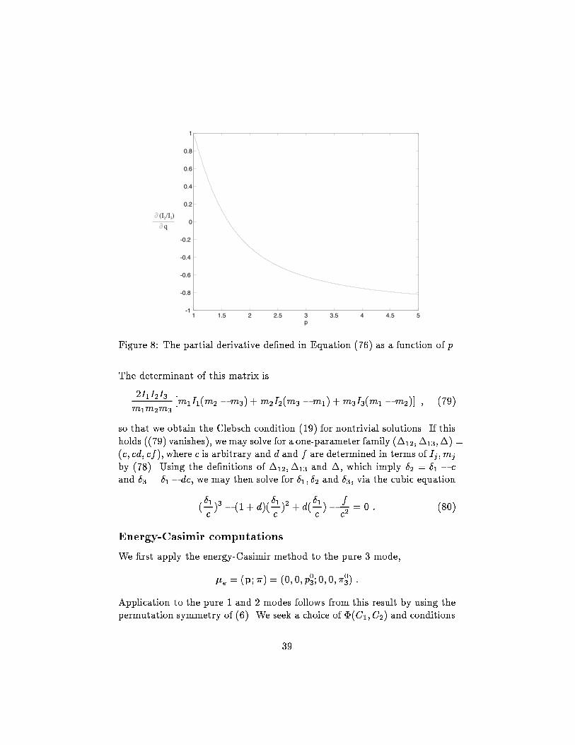
Figure 8: The partial derivative de�ned in Equation (76) as a function of p.The determinant of this matrix is2I1I2I3m1m2m3 [m1I1(m2 �m3) +m2I2(m3 �m1) +m3I3(m1 �m2)] ; (79)so that we obtain the Clebsch condition (19) for nontrivial solutions. If thisholds ((79) vanishes), we may solve for a one-parameter family (�12;�13;�) =(c; cd; cf), where c is arbitrary and d and f are determined in terms of Ij ; mjby (78). Using the de�nitions of �12;�13 and �, which imply �2 = �1 � cand �3 = �1�dc, we may then solve for �1; �2 and �3, via the cubic equation(�1c )3 � (1 + d)(�1c )2 + d(�1c )� fc2 = 0 : (80)Energy-Casimir computationsWe �rst apply the energy-Casimir method to the pure 3 mode,�e = (p;�) = (0; 0; p03; 0; 0; �03) :Application to the pure 1 and 2 modes follows from this result by using thepermutation symmetry of (6). We seek a choice of �(C1; C2) and conditions39

on p03, �03 such that, evaluated at �e, H� has �rst derivative equal to zeroand second derivative positive de�nite, whereH�(�) = H(�) + �(C1(�); C2(�))= 12(p �M�1p+ � � I�1�) + �(p � �; 12 jpj2) : (81)De�ne _� = @�@(p � �) ; �0 = @�@(12 jpj2) :The �rst derivative of H� isDH�(p;�) � (�p; ��) = (M�1p+ _�� + �0p) � �p (82)+ (I�1� + _�p) � �� :When evaluated at �e the �rst derivative is zero if and only if_�(p03�03 ; 12(p03)2) = � 1I3 �03p03!�0(p03�03 ; 12(p03)2) = � 1m3 + 1I3 �03p03!2 :Next we compute the second derivative of H�. Letq = �00(p03�03; 12(p03)2); u = ��(p03�03 ; 12(p03)2); w = _�0(p03�03 ; 12(p03)2) :The matrix of the second derivative at �e is0BBBBBBBB@ 1I1 0 0 _� 0 00 1I2 0 0 _� 00 0 a33 0 0 a36_� 0 0 1m1 + �0 0 00 _� 0 0 1m2 + �0 00 0 a36 0 0 a66 1CCCCCCCCA ; (83)where a33 = 1I3 + u(p03)2; a36 = _� + up03�03 + w(p03)2 ;a66 = 1m3 + �0 + u(�03)2 + wp03�03 + q(p03)2 ;40

and evaluation of derivatives of � at �e is implied. If the matrix (83) isde�nite, it is positive de�nite since the �rst principal determinant is positive,and it is positive de�nite if all six principal determinants are positive. Thesix principal determinants, denoted �i, i = 1; : : : ; 6, are�1 = 1I1 ; �2 = 1I1I2 ; �3 = a33 1I1I2 ;�4 = a33 1I2 � 1I1 � 1m1 + �0�� _�2� ;�5 = a33� 1I1 � 1m1 +�0�� _�2�� 1I2 � 1m2 +�0�� _�2� ;�6 = (a33a66 � a236)� 1I1 � 1m1 + �0�� _�2�� 1I2 � 1m2 +�0�� _�2� :If we take q = 1 and u = w = 0 and substitute in for _� and �0 from (82),positive de�niteness is assured if and only if for both i = 1 and i = 2� 1Ii � 1I3� 1I3 �03p03 !2 > 1Ii � 1m3 � 1mi� : (84)Thus, the pure 3 mode is Lyapunov stable if (84) is satis�ed. This followsfrom the energy-Casimir method where we have taken the function � to be�(C1; C2) = �C1 + �C2 + 12(C2 � �C2)2 ;where� = � 1I3 �03p03! ; � = � 1m3 + 1I3 �03p03!2 ; �C2 = C2(�e) = 12(p03)2 :Next we apply the energy-Casimir method to the 2{3 mixed mode,�e = (p;�) = (0; p02; p03; 0;��23I2p02;��23I3p03) ;where �23 = s m3 �m2m2m3(I2 � I3) :41

We again seek a choice of �(C1; C2) such that, evaluated at �e,H� describedby (81) has �rst derivative equal to zero and second derivative positive def-inite. When evaluated at �e, the �rst derivative is zero if and only if_�(C1(�e); C2(�e)) = ��23�0(C1(�e); C2(�e)) = �223I2 � 1m2 = �223I3 � 1m3 = m3I3 �m2I2m2m3(I2 � I3) :Let the second partials of � evaluated at �e be de�ned byq = �00(C1(�e); C2(�e)); u = ��(C1(�e); C2(�e)); w = _�0(C1(�e); C2(�e)) :The matrix of the second derivative evaluated at �e is0BBBBBBBB@ 1I1 0 0 ��23 0 00 1I2 + u(p02)2 up02p03 0 a25 a260 up02p03 1I3 + u(p03)2 0 a35 a36��23 0 0 1m1 +�0 0 00 a25 a35 0 a55 a560 a26 a36 0 a56 a66 1CCCCCCCCA ; (85)where a25 = ��23 + (u�23I2 + w)(p02)2a26 = (u�23I3 + w)p02p03a35 = (u�23I2 + w)p02p03a36 = ��23 + (u�23I3 + w)(p03)2a55 = 1m2 + �0 + (q + u�223I22 + 2w�23I2)(p02)2a56 = (q + u�223I2I3 + w(I2 + I3)�23)p02p03a66 = 1m3 + �0 + (q + u�223I23 + 2w�23I3)(p03)2 :If the matrix (85) is de�nite it is positive de�nite since the �rst principaldeterminant is positive. Let w = 0 and de�neE = 1I2I3 + u (p03)2I2 + (p02)2I3 ! ;F = 1I1 � 1m1 + �0�� �223 :42

Note that E > 0 if u > 0 and F > 0 since m2 > m1 and I2 > I1. The sixprincipal determinants of (85) are�1 = 1I1 ; �2 = 1I1 � 1I2 + u(p02)2� ; �3 = 1I1E; �4 = EF ;�5 = F (p02)2I2I3 (q + 4�223uI22 + quI2(p02)2 + quI3(p03)2) ;�6 = 4F �223I2I3 (I3 � I2)2qu(p02p03)2 :All principal determinants are positive, and therefore the matrix (85) ispositive de�nite, if we choose q > 0 and u > 0. For example, let q = u = 1,then �(C1; C2) = �C1 + �C2 + 12(C1 � �C1)2 + 12(C2 � �C2)2 ;where � = ��23; � = �223I2 � 1m2 = �223I3 � 1m3 ;�C1 = C1(�e) = �23(I2(p02)2 + I3(p03)2); �C2 = C2(�e) = 12((p02)2 + (p03)2) :By the energy-Casimir method the 2{3 mixed mode is Lyapunov stable.Melnikov computationsThe partial derivatives necessary for computation of the Melnikov integrand(70) may be expressed as follows:@0@r = 2Abr3 (1 + cos�)(2 �B + cos�)@0@� = Abr2 (2 �B � 1) sin�@H0@r = rI � 2A �Br ( �B + cos�)@H0@� = A �B r2 � b2r2 ! sin �@H�@r = �I r sin2 �I � �m a2bmr5 �C h(2b2 � r2) sin �(1 + cos �) + br cos � sin �i@H�@� = ��m a2mr4 �C(r2 � b2)(r cos � cos�� b sin � sin �) ; (86)43

where �C = b(1 + cos�) sin� + r sin � cos� :Here we have computed the \free" derivatives (as in the equations of motion(27)) and restricted to the unperturbed homoclinic level set. Evaluating the�rst term in parentheses in (70), we �nd:@H0@r @H�@� � @H0@� @H�@r = ��IA �B(r2 � b2)Ir sin � sin2 �+�m a2(r2 � b2) �CmIr3 (b sin� sin � � r cos � cos�)+�m a2bA �B(1� �B) �Cmr4 [b(1 + cos�) cos� � r sin � sin �] ; (87)while the second term gives@H0@r @0@� � @H0@� @0@r = Ab sin�Ir3 h(2 �B � 1)r2 � 2AI �B2(1 + cos �)i : (88)We note that this latter term is odd in t, while 0 is even. Using thesefacts and the odd/even properties inherent in (87), expressing powers andproducts of sin �; cos� via the double angle formulae, and expanding sin 2�as sin(2[�0 � ��(t)]) = sin 2�0 cos 2��(t)� cos 2�0 sin 2��(t)and cos 2� similarly, and recalling from its de�nition (69) that ��(t) is alsoodd, we may use the fact that odd functions of t vanish identically whenintegrated over the real line. This shows that all the integrand terms dropout except those multiplying sin 2�0, leading to the form of Equation (71).The explicit functions EI(t) and Em(t) are:EI(t) = A(r2 � b2)4I0r " b �DI0r2 + 2 �B# sin � sin 2�� ; (89)where �D = h(2 �B � 1)r2 � 2AI �B2(1 + cos�)i (90)(cf. (88)), andEm(t) = a2b2m0r �("br(1� �B)(1� 2 cos�) cos2�� � (b2(1� �B) + b2 � r2 �B) sin � sin 2��bI #44

+A �B(1� �B)(1 + cos�)r3 h(b2(1 + cos �)� r2(1� cos�)) cos2��+2br sin � sin 2��]� A �D sin �2I0r4 h(b2(1 + cos�)� r2(1� cos �)) sin2�� � 2br sin � cos 2��i) :(91)That the resulting integrals converge follows from the behavior of the unper-turbed solution (67) as jtj ! 1: speci�cally, r ! b; �B ! 1 and (1+cos�)!b2=2AI exponentially fast. Unfortunately, they do not seem to be com-putable in closed form; indeed, we cannot even explicitly solve (69) for ��(t).However, in the limit I1=I � 1, we have 0 � �b=I1 and �� � bt=I1, andthe expressions above simplify considerably. In particular, in EI we have�DI0r2 � 2 �B ;and ignoring the former term, the integral may be estimated asZ +1�1 EI(t)dt � �AI12bI Z +1�1 (r2 � b2)r �B sin � sin 2��dt : (92)>From the �rst component of the unperturbed equation (66) and the �rstexpression of (67), we haveA(r2 � b2)r �B sin � = rdrdt = b22 ddt " (4� �b2)(�b+ 2C(t))�b(2 + �bC(t))2 # ;substituting this into (92), integrating by parts and noting that the bound-ary terms vanish due to the exponential decay of the function in squarebrackets, we obtainb22I Z +1�1 "(4� �b2)(�b+ 2C(t))�b(2 + �bC(t))2 # cos(2btI1 )dt : (93)This expression may be evaluated by the method of residues to yield:Z +1�1 EI(t)dt � 2�sinh(�!) �bII1 cos(!�) +pAI sin(!�)� ; (94)where ! = 2bII1p4AI � b2 ; � = ln "p4AI +p4AI � b2b # :We conclude that, for I1=I � 1, the EI integral is nonzero except at isolatedparameter values. 45