EC 8751 – OPTICAL COMMUNICATION

UNIT IV OPTICAL RECEIVER, MEASUREMENTS AND COUPLING

Fundamental receiver operation-preamplifiers-digital signal transmission-error sources-Front end

amplifiers-digital receiver performance-probability of error-receiver sensitivity-quantum limit.

Optical power measurement-attenuation measurement-dispersion measurement- Fiber Numerical

Aperture Measurements- Fiber cut- off Wave length Measurements- Fiber diameter measurements-

Source to Fiber Power Launching-Lensing Schemes for Coupling Management-Fiber to Fiber Joints-

LED Coupling to Single Mode Fibers-Fiber SplicingOptical Fiber connectors.

FUNDAMENTALS OF RECEIVER OPERATION:

The function of the optical transmitter is to convert the electric signal to an optical

signal.

The transmitted signal is a two-level binary stream consisting of either a 0 (absence of

light pulse) or 1 (presence of light pulse) in a timeslot of duration Tb.

As the optical signal propagates along the fiber , it gets attenuated and distorted.

Fig. Signal path through an optical data link

Fig. Basic sections of an optical receiver

Upon reaching the end of the fiber, the receiver converts the optical signal back to an

electrical signal. The basic components of an optical receiver is shown below.

The PIN or APD produces an electric current that is proportional to the received

power level.

Since the electric current thus produced is very weak, a front-end amplifier is used to

boost up the signal.

After amplification, the signal passes through a low-pass filter to reduce the noise that

is outside the signal bandwidth.

To reduce the effect of ISI and to reshape the pulses, equalizer is used.

The sampling circuit samples the signal level at the midpoint of each time slot.

The decision circuit compares it with a certain reference voltage known as the

threshold level.

If the received signal level is greater than the threshold level, 1 is said to have been

received and if it is below the threshold , 0 is said to have been received.

The clock recovery or timing recovery circuit generates a periodic clock signal with a

periodicity equal to the bit interval which helps the receiver to know about the bit

boundaries.

RECEIVER SENSITIVITY

Optical communication systems use a BER value to specify the performance

requirements for a particular transmission link application. To achieve a desired BER at a

given data rate, a specific minimum average optical power level must arrive at the

photodetector. The value of this minimum power level is called the receiver sensitivity.

PREAMPLIFIER:

The bandwidth, BER, noise and sensitivity of optical receiver are determined

by preamplifier stage. Preamplifier circuit must be designed with the aim of optimizing these

characteristics. Commonly used preamplifier in optical communication receiver are

1. Low – impedance preamplifier (LZ)

2. High – impedance preamplifier (HZ)

3. Transimpedance preamplifier (TZ)

1. LOW – IMPEDANCE PREAMPLIFIER (LZ):

In low-impedance preamplifier, the photodiode is configured into low – impedance

amplifier. The bias resister bR is used to match the amplifier impedance. bR along with the

input capacitance of amplifier decides the bandwidth of amplifier. The total preamplifier load

resistance RL = RaRb / (Ra + Rb) is the parallel combination of Ra and Rb. The value of the

bias resistor, in conjunction with the amplifier input capacitance, is such that the preamplifier

bandwidth is equal to or greater than the signal bandwidth. Low – impedance preamplifier

can operate over a wide bandwidth but they have poor receiver sensitivity. Therefore the low

– impedance amplifiers are used where sensitivity is of not prime concern.

2. HIGH– IMPEDANCE PREAMPLIFIER (HZ):

In high – impedance preamplifier the objective is to minimize the noise from all sources.

This can be achieved by –

- Reducing input capacitance by selecting proper devices.

- Selecting detectors with low dark currents.

- Minimizing thermal noise of biasing resistors.

- Using high impedance amplifier with large bR .

The high impedance amplifier impedance amplifier uses FET or a BJT. As the high

impedance circuit has large RC time constant, the bandwidth is reduced. The above figure

shows the equivalent circuit of high input pre-amplifier.

High-input impedance preamplifiers are most sensitive and find applications in long –

wavelength, long haul routes. The high sensitivity is due to the use of a high input resistance

(typically > 1 MΩ), which results in exceptionally low thermal noise. The combination of

high resistance and receiver input capacitance, results in very low BW, typically < 30 kHz,

and this causes integration of the received signal. A differentiating, equalizing or

compensation network at the receiver output corrects for this integration

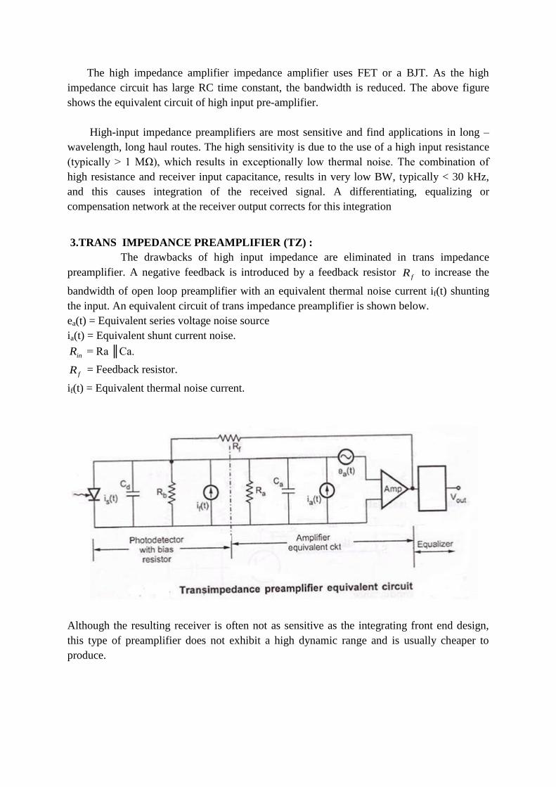
3.TRANS IMPEDANCE PREAMPLIFIER (TZ) :

The drawbacks of high input impedance are eliminated in trans impedance

preamplifier. A negative feedback is introduced by a feedback resistor fR to increase the

bandwidth of open loop preamplifier with an equivalent thermal noise current if(t) shunting

the input. An equivalent circuit of trans impedance preamplifier is shown below.

ea(t) = Equivalent series voltage noise source

ia(t) = Equivalent shunt current noise.

inR = Ra ║Ca.

fR = Feedback resistor.

if(t) = Equivalent thermal noise current.

Although the resulting receiver is often not as sensitive as the integrating front end design,

this type of preamplifier does not exhibit a high dynamic range and is usually cheaper to

produce.

QUANTUM LIMIT

The minimum received power level required for a specific BER of digital system is

known as Quantum limit.

ERROR SOURCES:

Errors in the detection mechanism can arise from various noises and disturbances

associated with the signal detection system.

The two most common examples of the spontaneous fluctuations are shot noise and

thermal noise.

Shot noise arises in electronic devices because of the discrete nature of current flow

in the device.

Thermal noise arises from the random motion of electrons in a conductor.

The random arrival rate of signal photons produces a quantum (or shot) noise at the

photo detector. This noise depends on the signal level.

This noise is of particular importance for PIN receivers that have large optical input

levels and for APD receivers.

When using an APD, an additional shot noise arises from the statistical nature of the

multiplication process. This noise level increases with increasing avalanche gain M.

Thermal noises arising from the detector load resistor and from the amplifier

electronics tend to dominate in applications with low SNR when a PIN photodiode is

used.

When an APD is used in low-optical-signal level applications, the optimum avalanche

gain is determined by a design tradeoff between the thermal noise and the gain-

dependent quantum noise.

The primary photocurrent generated by the photodiode is a time-varying Poisson

process.

If the detector is illuminated by an optical signal P(t), then the average number of

electron-hole pairs generated in a time t is

0

)(h

EtP

hN

where,

is the detector quantum efficiency, h is the photon energy, and E is the energy received

in a time interval .

The actual number of electron-hole pairs n that are generated fluctuates from the

average according to the Poisson distribution

where,

Pr(n) is the probability that n electrons are emitted in an interval

For a detector with a mean avalanche gain M and an ionization rate ratio k, the

excess noise factor F(M) for electron injection is

where,

The factor x ranges between 0 and 1.0 depending on the photodiode material.

A further error source is attributed to intersymbol interference (ISI), which results

from pulse spreading in the optical fiber.

The fraction of energy remaining in the appropriate time slot is designated by , so

that 1- is the fraction of energy that has spread into adjacent time slots.

RECEIVER CONFIGURATION

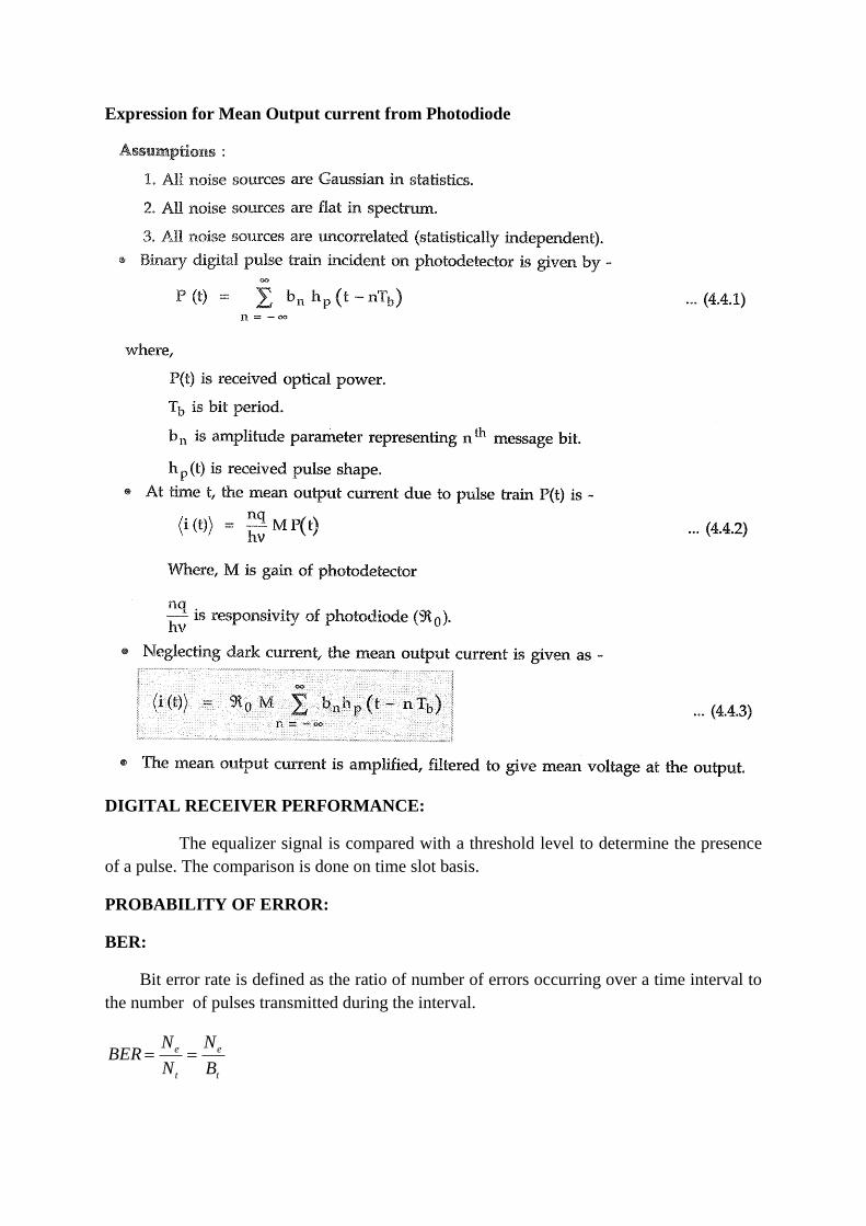
Expression for Mean Output current from Photodiode

DIGITAL RECEIVER PERFORMANCE:

The equalizer signal is compared with a threshold level to determine the presence

of a pulse. The comparison is done on time slot basis.

PROBABILITY OF ERROR:

BER:

Bit error rate is defined as the ratio of number of errors occurring over a time interval to

the number of pulses transmitted during the interval.

t

e

t

e

B

N

N

NBER

Where bT

B1

is the bit rate.

Typical error rates for optical fiber communication ranges from 10-9

to 10-12

.

This error rate depends on the SNR at the receiver.

To compute BER at the receiver ,probability distribution function of the signal at the

equalize output should be known.

Noise power for logic 0 ≠ noise power for logic 1.

CONDITIONAL PDF:

P

x

y is the probability that the output voltage is ‘y’ when ‘x’ was transmitted.

The functions

1

yp and

0

yp are conditional PDF

)1(1

1

dyy

PVP

V

is the Probability that output voltage <threshold when logic

‘1’ is sent.

)2(0

0

dyy

PVPv

is the Probability that output voltage >threshold when logic

‘0’ is sent.

If the threshold voltage is vth , then

ththe VbPVaPP 01

Where ‘a’ and ‘b’ are the probabilities that either a ‘1’ or ‘0’ occurs respectively and

are determined by a priori distribution of the data.

The probability that measured sample s(t1) falls in the range s to s+ds is

)3(2

1 2

2

2

)(

dsedssfms

2;)( PDFSf noise variance.

Mean of Gaussian output for ’1’=bon.

Mean of Gaussian output for ’0’=boff.

variance of Gaussian output for ’1’= 2

on .

variance of Gaussian output for ’0’= 2

off .

Probability of error PO(V)=equalizer output voltage between vth and ∞.

thvvth

th dyyfdyy

PVP 000

thv off

off

off

th dvbv

VP )4(2

)(exp

2

12

2

0

Probability of error P1(V)=equalizer output voltage between -∞ and vth.

thth vv

th dyyfdyy

PVP 111

thv

on

on

on

th dvvb

VP )5(2

)(exp

2

12

2

1

From (4)

thv off

off

off

the dvbv

VPP2

2

02

)(exp

2

1

Vth=2

v

Let 2

2

2

2

)(y

off

bv off

222 2)( ybv offoff

22

22

1

2222

22

2

,)(

2

2

2

v

y

e

off

off

thoff

off

offoff

offoff

dyeP

vor

vy

yv

vvbwhenv

ybv

when

dybvd

ybv

(Using standard result)

)8(

221

2

1

)(1)(

)7(222

1

),(2

)6(2

2

1

1

2

2

2

22

22

verfP

uerfuerfc

verfcP

uerfcdye

dyeP

dye

e

e

u

y

v

y

e

v

y

MEASUREMENTS:

1.REFRACTIVE INDEX PROFILE MEASUREMENT:

Refractive index profile of the fiber core is an important parameter that determines the

characteristics of optical fibers.

Numerical aperture of the fiber, number of modes propagating within the core can be

determined from refractive index profile.

INTERFEROMETRIC METHOD:

It is widely used to determine the refractive index profiles of optical fibers.

There are two methods used. They are

1.Transmitted light interferometer(Mach-Zender).

2.Reflected light interferometer(Michelson).

MACH-ZENDER METHOD:

A sample slice of fiber is taken and both ends are polished to obtain smooth and

optically flat surface.

Slab is immersed in index matching fluid and examined with interference microscope.

Light from laser source is passed through beam splitter.

The function of beam splitter is to split the incoming beam into transmitted beam and

reflected beam based on splitting ratio.

Two mirrors M1 & M2 are used, one for reflecting the transmitted beam towards fiber

slab and the other for reflecting the reflected beam from the beam splitter, to be

viewed through the microscope.

Optical rays from M1, are passed through the fiber slab.

Since refractive index is inversely proportional to density ( )1

density of the

material, as the density of the fiber core material varies, light traces different paths of

different wavelengths.

This is observed through an electronic microscope.

Phase of the incident light through M2 is compared with the phase of emerging light

from the slab via M1.

Interference fringe pattern is observed through microscope.

Fringe displacement(q), if any due to variation in density of the core material is noted.

Refractive index difference is given by,

x

qn

------(1)

where, q=fringe shift.

=incident optical wavelength.

x=thickness of the fiber slab.

n =refractive index difference.

Graph is plotted with core radius along x-axis & n along y axis.

The values of n is obtained from equation(1).

And from the graph it is noted that the profile of the sample is graded-index profile.

GRAPH

ADVANTAGES:

Accurate measurement.

Detailed knowledge on refractive index profile.

DISADVANTAGES:

Time required to prepare slab is more.

Computation is tedious.

NEAR FIELD SCANNING METHOD:

Near field scanning method determines refractive index profile from intensity

distribution.

Lambertain source(LED or Tungsten filament source) is used to execute all guided

modes.

Light rays from Lambertain source is coupled into the fiber.

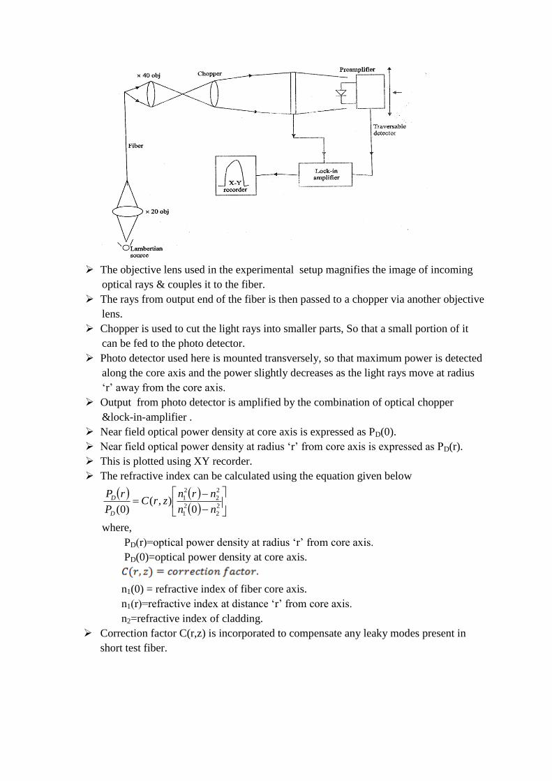
The objective lens used in the experimental setup magnifies the image of incoming

optical rays & couples it to the fiber.

The rays from output end of the fiber is then passed to a chopper via another objective

lens.

Chopper is used to cut the light rays into smaller parts, So that a small portion of it

can be fed to the photo detector.

Photo detector used here is mounted transversely, so that maximum power is detected

along the core axis and the power slightly decreases as the light rays move at radius

‘r’ away from the core axis.

Output from photo detector is amplified by the combination of optical chopper

&lock-in-amplifier .

Near field optical power density at core axis is expressed as PD(0).

Near field optical power density at radius ‘r’ from core axis is expressed as PD(r).

This is plotted using XY recorder.

The refractive index can be calculated using the equation given below

2

2

2

1

2

2

2

1

0),(

)0( nn

nrnzrC

P

rP

D

D

where,

PD(r)=optical power density at radius ‘r’ from core axis.

PD(0)=optical power density at core axis.

n1(0) = refractive index of fiber core axis.

n1(r)=refractive index at distance ‘r’ from core axis.

n2=refractive index of cladding.

Correction factor C(r,z) is incorporated to compensate any leaky modes present in

short test fiber.

GRAPH

ADVANTAGES:

Straight forward method.

Rapid technique.

DISADVANTAGES:

Implementing correction factor C(r,z) is time consuming.

Mode coupling differential mode attenuation can lead to error in measurements.

END REFLECTION METHOD:

Refractive index at any point in cross section of optical fiber is related to reflected

power from fiber surface at that point , based on Fresnel reflection formula.

Fraction of light reflected at air fiber interface is

2

1

1

1

1power) opticalcident power)/(In optical (Reflected

n

nr

where,

n1=Refractive index at point on fiber surface .

PROCEDURE:

Laser beam is directed through a polarizer and 4

plate to prevent feedback of

reflected optical power.

Circularly polarized light from 4

plate is filtered and expanded to provide suitable

spot size.

The function of beam splitter is to split the incoming beam into transmitted beam &

reflected beam based on splitting ratio.

Reflected beams are used for measurements through PIN diodes , and lock in

amplifier.

Reflected power is monitored as function of position on X-Y recorder.

Reflections from another end unobserved face are minimized by using index matching

gel.

DISADVANTAGES:

Fiber alignment is necessary.

Fiber end face should be perfectly flat ,else it can cause reflections.

2.MEASUREMENT OF NUMERICAL APERTURE:

The numerical aperture is an important optical fiber parameter which determines the

light gathering capability of optical fiber.

This in turn can be need to determine normalized frequency and number of modes

propagating within the fiber.

The numerical aperture(NA) is given by

2

2

2

1 nnSinNA a for step index fiber and

2

2

2

1 )( nrnSinNA a for graded index fiber, since ‘n’ increases radically.

TRIGNOMETRIC METHOD FOR STEP-INDEX FIBER:

The experimental setup for calculating numerical aperture(NA) or step index fiber

using trigonometric method is shown.

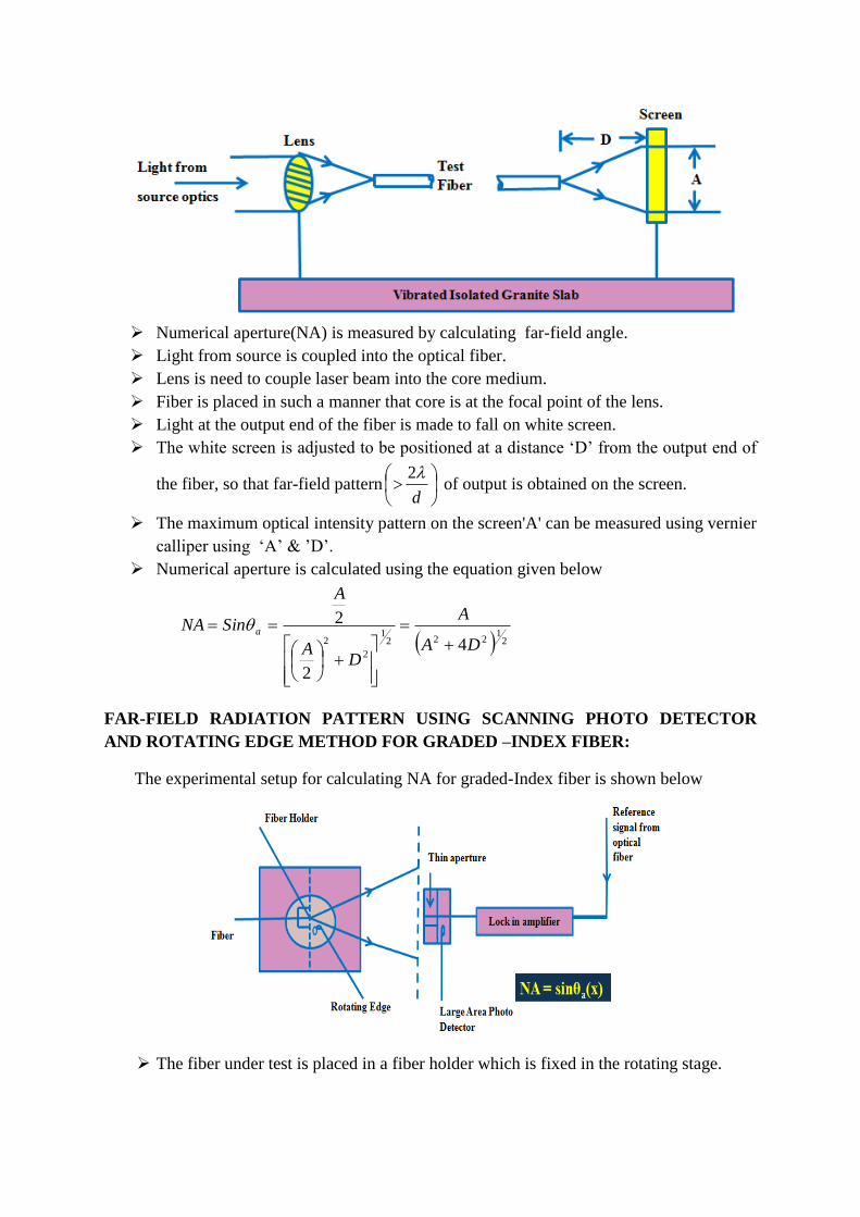
Numerical aperture(NA) is measured by calculating far-field angle.

Light from source is coupled into the optical fiber.

Lens is need to couple laser beam into the core medium.

Fiber is placed in such a manner that core is at the focal point of the lens.

Light at the output end of the fiber is made to fall on white screen.

The white screen is adjusted to be positioned at a distance ‘D’ from the output end of

the fiber, so that far-field pattern

d

2 of output is obtained on the screen.

The maximum optical intensity pattern on the screen'A' can be measured using vernier

calliper using ‘A’ & ’D’.

Numerical aperture is calculated using the equation given below

21

2221

2

2 4

2

2

DA

A

DA

A

SinNA a

FAR-FIELD RADIATION PATTERN USING SCANNING PHOTO DETECTOR

AND ROTATING EDGE METHOD FOR GRADED –INDEX FIBER:

The experimental setup for calculating NA for graded-Index fiber is shown below

The fiber under test is placed in a fiber holder which is fixed in the rotating stage.

The output end of the fiber is positioned on the rotating stage with its far end parallel

to the plane of the photo detector input.

The photo detector is placed 10 to 20 cm from the fiber and is positioned in order to

obtain maximum signal with rotation (i.e) 0 .

Output power is observed and plotted as a function of angle.

Reference signal from optical fiber is given to Lock-in-amplifier and the output of

photo detector is also fed to Lock-in-amplifier.

The Lock-in-amplifier only amplifies the wavelength that matches with the

wavelength of reference light signal.

The angle at which the photodetector detects maximum signal power is measured as

acceptance angle.

NA is calculated using the equation xNA asin

3.FIBER DIAMETER MEASUREMENT:

The fiber outer diameter is measured using fiber image projection (shadow method) as

shown below,

Laser beam from the He-Ne laser source is collimated using two lenses G1 & G2.

It is then reflected from two mirrors M1 & M2.

The mirror M2 is fixed to a galvanometer which makes it to rotate through a small

angle at a constant angular velocity.

The mirror velocity dt

d is noted by means of galvanometer.

The reflected light from mirror M2 is focused in the plane of the fiber by a lens and

the shadow is made to fall on photo detector.

The velocity of the fiber shadow is noted as dt

ds which is directly proportional to the

mirror velocity.

ldt

ds

dt

d

Where ‘l’ is the distance between the mirror and the photo detector.

dt

d is the mirror velocity.

dt

ds is the shadow velocity.

The sweep circuit in the set up is used to generate saw tooth signal which when given

to galvanometer makes the pointer to deflect.

The output electrical pulse from photo detector and reference electrical pulse from

pulse generator are given to op-amp summing amplifier.

The summing amplifier amplifies the output pulses from the photo-detector according

to the reference pulses from pulse generator.

The width of the pulse is calculated using time interval detector.

The electrical pulse width we of the shadow is related to the fiber outer diameter d0 as

given below

d0= wedt

ds

The fiber outer diameter thus determined is then recorded on the printer.

CORE DIAMETER:

The technique used for determining the refractive Index profile can be used to

measure the core diameter.

But for graded index fiber, it is difficult because the refractive index varies radially.

Core diameter measurement is also possible from the near field pattern of a suitably

illuminated all guided modes excited fiber.

The measurements may be taken using a microscope equipped with a micrometer

eyepiece.

4. FIBER CUTT-OFF WAVELENGTH MEASUREMENT:

Multimode fiber has many cut-off wavelengths because the number of bound

propagating modes is usually large.

The number of guided modes is given by,

2

2

2

1

2

nna

M g

Where,

a=core radius.

n1=core refractive index

n2=cladding refractive index.

The cut-off wavelength of a 11LP mode is the maximum wavelength for which the

mode is guided by the fiber.

The configurations for single turn and split mandrell is shown below.

In the bending-reference technique the power SP transmitted through the fiber

sample is measured as a function of wavelength.

SP corresponds to total power.

The smaller transmitted power bP is measured.

bP corresponds to the fundamental mode power.

The bend attenuation ba ,which is the difference between total power and

fundamental power is calculated as

b

Sb

P

Pa 10log10

A graph is plotted with wavelength along x-axis and bend attenuation along y-axis.

The effective cut-off wavelength ce is determined from the graph, which is the

longest wavelength at which bend attenuation ba equals 0.1dB.

5. DISPERSION MEASUREMENT:

When light pulses travel along a fiber, the width of the pulses get broadened.

This broadening of pulses is called dispersion. This is because the light pulses spread as

they propagate along the length of the fiber. It causes overlapping of pulses leading to

Intersymbol Interference(ISI) which limits information carrying capacity of fiber.

TIME DOMAIN DISPERSION MEASUREMENT:

Any system needs certain input to give corresponding output. Consider a fiber

optic cable as a system with impulse t at input.

dhtPtP

T

T

inout

2

2

Pout(t)= h(t) * Pin(t)

The impulse signal has negligible pulse width. If that impulse signal is given

as input to fiber optic cable, due to dispersive effect, the pulse gets broadened in time

domain and impulse response h(t) is obtained as shown. This is called time domain

dispersion which is measured in picoseconds or nanoseconds.

The experimental setup is shown

below:

Narrow optical pulse is injected into one end of the fiber and broadened output is detected

at the other end.

The power emitted from laser source varies for different modes. To make it uniform

mode scrambler is used.

One end of the fiber under test is connected to mode scrambler and other end is connected

to optical sampling oscilloscope which has inbuilt APD detector.

The width of the optical pulse is measured.

Then test fiber is replaced with short reference fiber which is lesser in length than test

fiber and the width of the pulse is measured.

The relative pulse amplitude for different pulse width parameter are measured.

Variable delay is used to adjust the difference in delay between test fiber and short

reference fiber.

FREQUENCY DOMAIN FREQUENCY MEASUREMENT

Optical signal is coupled through a mode scrambler to the test fiber.

At the output, photo detector measures Pout(f).

Input Pin(f) is then measured by replacing test fiber with a short reference fiber.

Output spectrum and input spectrum are compared using a spectrum analyser.

fP

fPfHthF

in

out

As modulation frequency increases, the output-optical power level decreases.

Optical bandwidth or fiber bandwidth is defined as the lowest frequency at which H(f)

reduces to 0.5.

6. FIBER ATTENUATION MEASUREMENTS:

Fiber attenuation measurement techniques are used to determine the total fiber

attenuation loss due to both absorption losses and scattering losses.

The common techniques used are

1. Cut-back method

2. Insertion loss method.

CUT-BACK METHOD:

The experimental setup for measurement of overall attenuation is shown below.

Light from white light source is focused to a lens and chopper and is given to lock-

in-amplifier.

Monochromator is used to select the required wavelength at which attenuation is

measured.

Microscopic objective lens is used to filter the light before being passed into the

fiber.

Mode scrambling device is usually attached to the fiber to get uniform distribution of

power.

Mode stripper is employed so that only the fundamental mode is allowed to

propagate along the fiber.

The optical fiber power is detected using PIN or avalanche photodiode at the

receiver.

Photo detector surface is usually index matched to the fiber output end face using

epoxy resin or index matching gel.

Finally the electrical output from the photo detector is fed to lock-in-amplifier, the

output of which is recorded.

The lock-in-amplifier performs phase-sensitive detection.

To find the transmission loss, the optical power is first measured at the output or far

end of the fiber.

The fiber is cut-off a few meters from the source and the output power at this end is

measured without distributing the input condition.

Attenuation ‘α’ in decibels per kilometre is expressed as

02

0110

21

log10

p

p

LLdB

Where,

L1=Original length of the fiber.

L2=cut back length of the fiber.

P01=output power at near end.

P02=output power at far end.

INSERTION LOSS METHOD:

Cut-back method cannot be used for cables with connectors. Hence insertion loss

method is used. This is less-accurate than cut back method.

The launch and detector couplings are made through connectors.

In case of multimode fibers, a mode scrambler is used to ensure that fiber core

contains equilibrium mode distribution.

In case of single mode fibers, cladding mode stripper is used to allow only

fundamental mode to propagate along the fiber.

The connector of short length launching fiber is attached to the connector of the

receiving system and the launch power level 1P is recorded.

Next the cable assembly to be tested is connected between the launching and

receiving systems and the received power level 2P is recorded.

Attenuation in decibels is calculated as

2

1log10p

pA

POWER LAUNCHING AND COUPLING

Source to Fiber Power Launching

Source Output Pattern

Lensing Schemes

• Lensing Schemes are used to improve the optical source to fiber coupling efficiency.

• Several Possible lensing schemes are:

1. Rounded end fiber 2. Non imaging Microsphere (small glass sphere in contact with both the fiber and source) 3. Imaging sphere ( a larger spherical lens used to image the source on the core area of the fiber end) 4. Cylindrical lens (generally formed from a short section of fiber) 5. Spherical surfaced LED and spherical ended fiber 6. Taper ended fiber

Fiber Alignment and Joint loss:

When the two jointed fiber ends care smooth and perpendicular to the fiber axes and

the two fiber axes perfectly aligned, a small portion of light may be reflected back

into the transmitting fiber causing attenuation at the joint. This phenomenon is known

as Fresnel reflection.

Fresnel formula r =

2

1

1

nn

nn

Where r – fraction of light reflected

n1- Core refract index

n – refractive index of medium

loss in decibels is due to Fresnel reflection at a single interface is given by,

LOSSfres = -10log10 (1-r)

Fresnel reflection may give a significant loss at a fiber joint.

The effect of Fresnel reflection at a fiber – fiber connection can be reduced to a very

low level through the use of an index matching fluid has the same refractive index as

the fiber core, losses due to Fresnel reflection are eradicated.

There are inherent connection problems when jointing fibers

- Different core and cladding diameters.

- Different numerical apertures and/or relative refractive index differences.

- Different refractive index profiles.

- Fiber faults.

The losses caused by the above factors together with those of Fresnel reflection are

usually referred to as intrinsic joint losses.

Misalignment may occur in 3 ways

- The separation between the fibers.

- The offset perpendicular to the fiber core axes.

- The angle between the core axes.

Optical losses due to 3 types of misalignment:

- depend upon the fiber type.

- Core diameter.

- Distribution of the optical power b/w propagating modes.

Various types of misalignment

1. Longitudinal misalignment

2. Lateral misalignment

3. Angular misalignment.

Lateral misalignment gives significantly greater losses per unit displacement than the

longitudinal alignment.

The effect of an index matching fluid in the fiber gap causes increased losses with

angular misalignment.

Fig. Insertion loss characteristics for jointed optical fibers with various types of

misalignment.

Multimode fiber joints:

Lateral misalignment reduces the overlap region between the two fiber cores.

The lateral coupling efficiency for two similar step index fibers

2

1

4

1

2

1

21

2cos2.

1.

/1

/16

a

y

a

y

a

y

nn

nnlat

Where n1 – Core refractive index

n - refractive index of medium

g - lateral offset of the fiber core axes

a - fiber core radius.

Lateral misalignment loss in dB

LOSSlat = -10log10ηlat dB

Lateral misalignment loss in multimode graded index fibers assuming a uniform

distribution of optical power throughout all guided was calculated by Gloge formula.

Lateral misalignment loss was dependent on the refractive index gradient α for small

lateral offset.

1

22

a

yLt for ay 2.00

Lateral coupling efficiency tlat L1

For graded index fiber, If α = 2, ayayLt /85.0/3

8

.

Lateral misalignment loss if both guided & leaky modes are included means

a

yLt 75.0

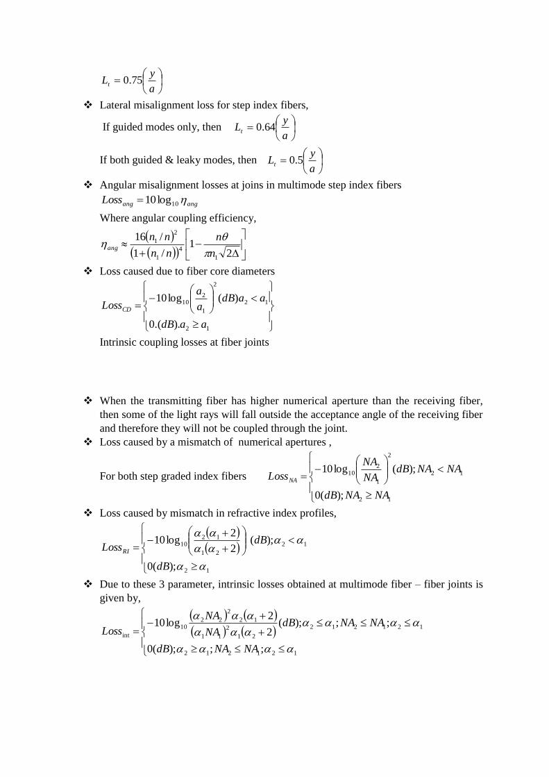
Lateral misalignment loss for step index fibers,

If guided modes only, then

a

yLt 64.0

If both guided & leaky modes, then

a

yLt 5.0

Angular misalignment losses at joins in multimode step index fibers

angangLoss 10log10

Where angular coupling efficiency,

21

/1

/16

1

4

1

2

1

n

n

nn

nnang

Loss caused due to fiber core diameters

12

12

2

1

210

)..(0

)(log10

aadB

aadBa

a

LossCD

Intrinsic coupling losses at fiber joints

When the transmitting fiber has higher numerical aperture than the receiving fiber,

then some of the light rays will fall outside the acceptance angle of the receiving fiber

and therefore they will not be coupled through the joint.

Loss caused by a mismatch of numerical apertures ,

For both step graded index fibers

12

12

2

1

210

);(0

);(log10

NANAdB

NANAdBNA

NA

LossNA

Loss caused by mismatch in refractive index profiles,

12

12

21

1210

);(0

);(2

2log10

dB

dBLossRI

Due to these 3 parameter, intrinsic losses obtained at multimode fiber – fiber joints is

given by,

121212

121212

21

2

11

12

2

2210

int

;;);(0

;;);(2

2log10

NANAdB

NANAdBNA

NA

Loss

Single mode fiber joints

Loss occurred in the absence of angular misalignment,

.17.2

2

dBy

Tt

Where spot size

2

879.2619.165.0 65.1

vvam

Insertion loss, .17.2

2

1 dBaNA

vnTa

Fiber splicing

Permanent joint between two fiber – fiber splice.

Process of joining two fibers is called as splicing.

Create long optical links.

No need of frequent connection and disconnection.

Factors to be considered

(i) Geometrical difference b/w two fibers.

(ii) Fiber misalignments at the joint.

(iii) Mechanical strength of the splice.

Splicing techniques

(i) Fusion splice.

(ii) V-Groove mechanical splice.

(iii) Elastic tube splice.

Before splicing or connecting the fiber, fiber end face propagation is the first step.

Fiber end must to be

- Flat

- ┴r to the fiber axis

- Smooth

Initial techniques used are

- Sawing

-

Polishing

Grinding - require lab to this. → Refer page no. 16 – (1).

Influences on fusion process

1. Self – centering effect: Tendency of the fiber to form a homogenous joint.

2. Core Eccentricity – Process of alignment the fiber cores.

3. Fiber and face quality – when cleaving, the fiber end faces has to be clean,

unchipped, flat & ┴r to be fiber axis.

4. Fiber propagation quality – when preparing the fibers for splicing, no damage

should occur to the fiber cladding.

- Any damage to this can produce microcracks during

splicing.

5. Dirt particles – Any contamination on the fiber cladding can lead to bad fiber

positioning

6. Fiber melting characteristics – when elastic are melts the fiber, the glass tends to

Collapse filling the gap with air or gas bubbles.

- therefore, Electric are should not be too intense or

weak.

7. Electrode condition – Electrode cleaning or replacement is necessary from time to

time.

Fusion splicing

Thermal bonding of two prepared fiber ends.

Two fiber ends are butted together which is then heated with an electric arc or a laser

pulse so that the ends are melted and bonded together.

Produce very low splice losses (Range – 0.05 to 0.1 dB )

The chemical changes during melting sometimes produce weak splice.

Controlled fracture techniques are used to cleave the fiber.

Highly smooth & ┴r end faces can be produced.

Requires a careful control of the curvature &the tension.

Improperly controlled tension can cause multiple fracture & can leave a lip or hacked

portion.

V – groove splicing

The prepared fiber ends are butted together in a V – shaped groove.

They are bonded with an adhesive or held in place by means of a cover plate .

The V- shaped channel is either grooved silicon, plastic ceramic or metal substrate.

Splice loss depends on the fiber size and eccentricity.

Elastic Tube Splicing

Automatically performs lateral, longitudinal and angular misalignment.

In splices, multi mode fibers give losses in the same range as commercial fusion

splice.

Loss equipment and skills are needed.

The device is made up of an elastic material.

Internal hole is of smaller diameter as compared to the fiber and is tapered at two fiber

ends for easy fiber insertion.

The fiber expands the hole diameter when it is inserted so that the elastic material

exerts a symmetrical force on the fibers.

This allows accurate and automatic alignment of axes of two fibers to be joined.

The fibers to be spliced do not have an equal diameter because each fiber mores into

position independently relative to the tube axis.

Splicing single –mode fibers

Lateral misalignment loss in single mode fibers

S

w

dL latSM

2

: explog10

spot size,w – mode-field radius; d – lateral displacement

This loss depends on the shape of the propagation mode.

Angular misalignment loss in single mode fibers

2

2: explog10

nL angSM

θ – angular displacement in radius; n2 – cladding refractive index.

Loss in SM fiber if there is gap

4

64log10

24

31

2

3

2

1:

Gnn

nnL gapSM

n3 → refractive index of medium b/w fibers.

Letting 2k

SG ; where S – longitudinal effect.

Optical fiber connectors An optical fiber connector terminates the end of an optical fiber, and enables

quicker connection and disconnection than splicing. The connectors mechanically

couple and align the cores of fibers so light can pass. Better connectors lose very

little light due to reflection or misalignment of the fibers. In all, about 100

different types of fiber optic connectors have been introduced to the market. An

optical fiber connector is a flexible device that connects fiber cables requiring a

quick connection and disconnection. Optical fibers terminate fiber-optic

connections to fiber equipment or join two fiber connections without splicing.

Hundreds of optical fiber connector types are available, but the key differentiator

is defined by the mechanical coupling techniques and dimensions. Optical fiber

connectors ensure stable connections, as they ensure the fiber ends are optically

smooth and the end-to-end positions are properly aligned. An optical fiber

connector is also known as a fiber optic connector. 1980s. Most fiber connectors

are spring loaded. The main components of an optical fiber connector are a

ferrule, sub-assembly body, cable, stress relief boot and connector housing. The

ferrule is mostly made of hardened material like stainless steel and tungsten

carbide, and it ensures the alignment during connector mating. The connector

body holds the ferrule and the coupling device serves the purpose of male-female

configuration The fiber types for fiber optic connectors are categorized into

simplex, duplex and multiple fiber connectors. A simplex connector has one fiber

terminated in the connector, whereas duplex has two fibers terminated in the

connector. Multiple fiber connectors can have two or more fibers terminated in

the connector. Optical fiber connectors are dissimilar to other electronic

connectors in that they do not have a jack and plug design. Instead they make use

of the fiber mating sleeve for connection purposes.

Common optical fiber connectors include

biconic, D4, ESCON, FC, FDDI, LC and SC.

• Biconic connectors use precision tapered ends to have low insertion loss.

• D4 connectors have a keyed body for easy intermateability.

• ESCON connectors are commonly used to connect from a wall outlet to a

device.

• FC connector (fixed connection connector) is used for single-mode fibers and

highspeed communication links.

• FDDI connector is a duplex connector which makes use of a fixed shroud.

• LC connector (local connection connector) has the benefit of small-form-factor

optical transmitter/receiver assemblies and is largely used in private and public

networks.

• SC connector (subscriber connector) is used in simplex and multiple

applications and is best suited for high-density applications.

Optical fiber connectors

Optical fiber connectors are used to join optical fibers where a

connect/disconnect capability is required. The basic connector unit is a connector

assembly. A connector assembly consists of an adapter and two connector plugs.

Due to the sophisticated polishing and tuning procedures that may be

incorporated into optical connector manufacturing, connectors are generally

assembled onto optical fiber in a supplier’s manufacturing facility. However, the

assembly and polishing operations involved can be performed in the field, for

example to make cross-connect jumpers to size. Optical fiber connectors are used

in telephone company central offices, at installations on customer premises, and

in outside plant applications. Their uses include: • Making the connection

between equipment and the telephone plant in the central office • Connecting

fibers to remote and outside plant electronics such as Optical Network Units

(ONUs) and Digital Loop Carrier (DLC) systems • Optical cross connects in the

central office • Patching panels in the outside plant to provide architectural

flexibility and to interconnect fibers belonging to different service providers •

Connecting couplers, splitters, and Wavelength Division Multiplexers (WDMs)

to optical fibers • Connecting optical test equipment to fibers for testing and

maintenance. Outside plant applications may involve locating connectors

underground in subsurface enclosures that may be subject to flooding, on outdoor

walls, or on utility poles. The closures that enclose them may be hermetic, or may

be “free-breathing.” Hermetic closures will prevent the connectors within being

subjected to temperature swings unless they are breached. Free-breathing

enclosures will subject them to temperature and humidity swings, and possibly to

condensation and biological action from airborne bacteria, insects, etc.

Connectors in the underground plant may be subjected to groundwater immersion

if the closures containing them are breached or improperly assembled. The latest

industry requirements for optical fiber connectors are in Telcordia GR-326,

Generic Requirements for Singlemode Optical Connectors and Jumper

Assemblies.A multi-fiber optical connector is designed to simultaneously join

multiple optical fibers together, with each optical fiber being joined to only one

other optical fiber.The last part of the definition is included so as not to confuse

multi-fiber connectors with a branching component, such as a coupler. The latter

joins one optical fiber to two or more other optical fibers.Multi-fiber optical

connectors are designed to be used wherever quick and/or repetitive connects and

disconnects of a group of fibers are needed. Applications include

telecommunications companies’ Central Offices (COs), installations on customer

premises, and Outside Plant (OSP) applications.The multi-fiber optical connector

can be used in the creation of a low-cost switch for use in fiber optical testing.

Another application is in cables delivered to a user with preterminated multi-fiber

jumpers. This would reduce the need for field splicing, which could greatly

reduce the number of hours necessary for placing an optical fiber cable in a

telecommunications network. This, in turn, would result in savings for the

installer of such cable.

Definition of Return Loss In technical terms, RL is the ratio of the light

reflected back from a device under test, Pout, to the light launched into that

device, Pin, usually expressed as a negative number in dB. RL = 10

log10(Pout/Pin) where is the reflected power and is the incident, or input, power.

Sources of loss include reflections and scattering along the fiber network. A

typical RL value for an Angled Physical Contact (APC) connector is about -

55dB, while the RL from an open flat polish to air is typically about -14dB. High

RL is a large concern in high bitrate digital or analog single mode systems and is

also an indication of a potential failure point, or compromise, in any optical

network.

PART – A

1. Define Quantum limit (Q). (May-June 2013) (R)

2. What are the error sources in fiber optic receiver? (May-June 2013, Nov-Dec 2012)

(R)

3. Define BER. (Nov-Dec 2016, April-May 2015) (R)

4. What is Cut-back method? (Nov-Dec 2016) (R)

5. List any two advantages of trans-impedance amplifiers. (Apr-May 2015) (U)

6. State the significance of maintaining the fiber outer diameter constant.(Nov-Dec

2014) (R)

7. Draw and describe the operation of fiber optic receiver. (Nov-Dec 2015) (U)

8. Mention few fiber diameter measurement techniques. (Nov-Dec 2015) (R)

9. A digital fiber optic link operating at 1310 nm, requires a maximum BER of 10-8

.

Calculate the required average photons per pulse. (Nov- Dec 2013) (U)

10. The photo detector output in a cutback attenuation set up is 3.3V at the far end of the

fiber. After cutting the fiber at the near end, 5 m from the far end, photo detector

output read was 3.92 V. What is the attenuation of fiber in dB/km? (Nov-Dec 2013) (U)

11. Define receiver sensitivity. (Nov-Dec 2017) (R)

12. Draw the generic structure of Transimpedance amplifier. (Nov-Dec 2017) (R)

13. Give some possible lensing schemes to improve optical source to fiber coupling

efficiency. (Nov-Dec 2012) (R)

Part – B

1. Explain the different methods employed in measuring the attenuation in optical fiber

with neat block diagram. (Nov-Dec 2016) (U)

2. What are the performance measures of a digital receiver? Derive an expression for bit

error rate of a digital receiver. (Nov-Dec 2016,Nov-Dec 2015) (AZ)

3. Explain how attenuation and dispersion measurements could be done. (Nov-Dec

2015, Nov-Dec 2013, Nov-Dec 2017) (U)

4. With a typical experimental arrangement, brief the measurement process of diameter

of the fiber. (Apr-May 2018) (U)

5. Draw the three types of front end optical amplifiers (preamplifiers) and

explain. (May-June 2013, Nov-Dec 2012, Nov-Dec 2013) (U)

6. Explain with a neat block diagram, the measurement of

a. Numerical aperture and acceptance angle. (Nov-Dec 2014, Nov-Dec 2017)

(U)

b. Refractive index profile. (Nov-Dec 2012, Nov-Dec 2014) (U)

7. With schematic diagram, explain the blocks and their functions of an optical

receiver. (Apr-May 2015, Nov-Dec 2014) (U)

8. A digital fibre optic link operationg at 850nm requires a maximum BER of

. Find the quantum limit in terms of the quantum efficiency of the

detector and the energy of the incident photon. (Apr-May 2015) (E)

9. Write detailed notes on the following. (May-June 2013) (U)

i. Fibre refractive index profile measurement.

ii. Fibre cut of wavelength measurement.

10. Write notes on cut-off wavelength measurement. (Nov-Dec 2012) (U)

11. Discuss the different structures of receiver in the optical fiber communication with

neat diagram. (Apr-May 2018) (U)

12. What is fiber splicing? Discuss about fusion splicing and mechanical splicing. (Nov-

Dec 2016, Apr-May 2018) (U)

13. Illustrate the different lensing schemes available to improve the power coupling

efficiency. (Apr-May 2018) (U)

14. What are the different types of fiber splices and misalignments. (R)

15. Describe the various types of fiber connectors and couplers. (May-June 2013) (U)

16. Explain fiber alignment and joint losses. (May-June 2013) (U)

17. Describe various fiber splicing techniques with their diagrams. (May-June 2013)

(U)

18. Describe the three types of fiber misalignment that contribute to insertion loss at an

optical fiber joint. (Nov-Dec 2014) (U)