Embed Size (px)
Citation preview

EUROPEAN ECONOMY
EUROPEAN COMMISSION DIRECTORATE-GENERAL FOR ECONOMIC
AND FINANCIAL AFFAIRS
ECONOMIC PAPERS
ISSN 1725-3187 http://europa.eu.int/comm/economy_finance
Number 246 March 2006
Economic spillover and policy coordination
in the Euro Area by
Klaus Weyerstrass, Johannes Jaenicke, Reinhard Neck, Gottfried Haber (Institute for Advanced Studies, Carinthia)
and Bas van Aarle, Koen Schoors, Niko Gobbin, Peter Claeys (Gent University)
Economic Papers are written by the Staff of the Directorate-General for Economic and Financial Affairs, or by experts working in association with them. The "Papers" are intended to increase awareness of the technical work being done by the staff and to seek comments and suggestions for further analyses. Views expressed represent exclusively the positions of the author and do not necessarily correspond to those of the European Commission. Comments and enquiries should be addressed to the: European Commission Directorate-General for Economic and Financial Affairs Publications BU1 - -1/13 B - 1049 Brussels, Belgium
ECFIN/000428 ISBN 92-79-01187-1 KC-AI-06-246-EN-C ©European Communities, 2006.

Economic Spillover and
Policy Coordination
in the Euro Area
Final Report Participating Institutions: Institute for Advanced Studies Carinthia (IHS Kärnten), Klagenfurt, Austria (Project Coordinator) CERISE, Ghent University, Ghent, Belgium
The study "Economic Spillover and Policy Coordination in the Euro Area" (tender
ECFIN/C/2004/01) was prepared by the Institute for Advanced Studies Carinthia (IHS
Kärnten) for the European Commission, Directorate General Economic and Financial Affairs.
The report was written by the following researchers involved in the project:
Klaus Weyerstrass, Johannes Jaenicke, Reinhard Neck, Gottfried Haber, Bas van Aarle,
Koen Schoors, Niko Gobbin and Peter Claeys.
The views expressed in this report represent exclusively the positions of the authors and do
not necessarily correspond to those of the European Commission.
Klagenfurt, November 2005

iv Contents
Table of Contents
List of Figures .......................................................................................................................... vi
List of Tables............................................................................................................................ ix
Executive Summary ................................................................................................................. x
1 Introduction and objectives............................................................................................ 1
PART 1: THEORY .................................................................................................................. 4
2 A working definition of spillover ................................................................................... 5 2.1 Introduction and literature overview................................................................................. 5 2.2 Foundation of empirical analysis.................................................................................... 16
PART 2: EMPIRICAL FINDINGS...................................................................................... 20
3 Budgetary spillover and short-term interest rates ..................................................... 22 3.1 Introduction..................................................................................................................... 22 3.2 Methodology and literature on fiscal and monetary policy analysis using VARs.......... 23 3.3 Fiscal spillover at the aggregate euro area level ............................................................. 25 3.4 Fiscal spillover in the euro area at the country level ...................................................... 34 3.5 Conclusions..................................................................................................................... 52 4 Budgetary spillover and long-term interest rates....................................................... 54 4.1 Introduction..................................................................................................................... 54 4.2 Deficits and interest rates: is there any robust evidence? ............................................... 55 4.3 A stock-flow fiscal VAR for open economies................................................................ 59 4.4 Crowding-out effects of fiscal policies........................................................................... 66 4.5 Spillover effects of fiscal policies................................................................................... 67 4.6 Summary and policy recommendations.......................................................................... 70 5 Budgetary stabilisation and the level of public debt .................................................. 88 5.1 Introduction..................................................................................................................... 88 5.2 A short overview of the literature ................................................................................... 88 5.3 The importance of the debt level: an empirical contribution.......................................... 93 5.4 Conclusion ...................................................................................................................... 99 6 Spillover from economic reform ................................................................................ 101 6.1 Introduction................................................................................................................... 101 6.2 Determination of mark-up ratios................................................................................... 103 6.3 The link between the mark-up and macroeconomic performance................................ 110 6.4 The influence of regulation on the mark-up ................................................................. 118 6.5 Summary of effects of structural reforms ..................................................................... 123

Contents v
7 Macroeconomic and welfare effects of structural and budgetary policies: spillover in the MSG3 model ...................................................................................... 125
7.1 Effects of structural policies ......................................................................................... 125 7.2 Budgetary consolidation policies.................................................................................. 133 7.3 Combined structural and budgetary consolidation policies.......................................... 148 7.4 Sensitivity analysis: monetary versus inflation targeting ............................................. 157 7.5 Welfare effects of structural and budgetary consolidation policies.............................. 163
PART 3: CONCLUSIONS .................................................................................................. 171
8 Summary, recommendations and future research................................................... 172
APPENDIX ........................................................................................................................... 182
Appendix 1a: Variables used for chapter 3 ............................................................................ 183
Appendix 1b: Spillover effects in VAR models (from chapter 3) ......................................... 185
Appendix 2a: Domestic economy: SVAR models with exogenous debt ratio. ..................... 201
Appendix 2b: SVAR models with yield................................................................................. 203
Appendix 2c: Data definitions and sources for chapter 4 ...................................................... 211
Appendix 3: The McKibbin-Sachs Global Model ................................................................. 212
Appendix 4: Impulse responses to a shock reducing the budget deficit in the MSG3 model ................................................................................................................. 215
Appendix 5: Spillover effects of combined structural and budgetary consolidation policies .......................................................................................................................... 251
Appendix 6: Variables used in chapter 6 ............................................................................... 279
References ............................................................................................................................. 280

vi List of Figures
List of Figures
Figure 1: Overview of spillover analysed in this study ......................................................... 17 Figure 2: Endogenous euro area variables in the euro area VAR.......................................... 26 Figure 3: Impulse response functions of macroeconomic shocks in the euro area model..... 29 Figure 4: Spillover from the (rest of the) euro area on individual countries
(France, Germany, Italy) ........................................................................................ 37 Figure 5: Spillover from Germany, France and Italy on the respective rest
of the euro area....................................................................................................... 46 Figure 6: Domestic economy, SVAR model (4.1a-b): impulse responses of real
long-term interest rates to shocks of 1% of GDP in net lending and debt ratio..... 73 Figure 7: Euro area economy, SVAR model (4.1a-b): impulse responses of real
long-term interest rates to shocks of 1% of GDP in net lending and debt ratio..... 75 Figure 8: Open economy, SVAR model (4.2a): on difference of country i to euro area;
impulse responses of real long-term interest rates to standard deviation shocks in the net lending and debt ratio ................................................................. 76
Figure 9: Open economy, "marginal method", SVAR model (4.2b): conditioned on euro area debt ratio; impulse responses of real long-term interest rates to shocks of 1% of GDP in net lending and debt ratio ............................................... 78
Figure 10: Open economy, "marginal method", SVAR model (4.2b): conditioned on euro area real long-term interest rate; impulse responses of real long-term interest rates to shocks of 1% of GDP in net lending and debt ratio...................... 80
Figure 11: Open economy, "marginal method", SVAR model (4.2b): conditioned on euro area debt ratio and euro area real long-term interest rates; impulse responses of real long-term interest rates to shocks of 1% of GDP in net lending and debt ratio................................................................................... 82
Figure 12: Quarterly EMU panel: the impact of tax changes on private consumption............ 96 Figure 13: Quarterly EMU panel: the impact of spending changes on private consumption .. 97 Figure 14: Yearly EMU panel: the impact of spending changes on private consumption....... 98 Figure 15: The ratio of debt to GDP: descriptive statistics, yearly EMU panel ..................... 99 Figure 16: Evolution of mark-up in selected euro area countries .......................................... 108 Figure 17: Evolution of mark-up in selected euro area countries, cont’d .............................. 108 Figure 18: Evolution of mark-up in the euro area, the US and the UK ................................. 109 Figure 19: TFP shift, Germany .............................................................................................. 128 Figure 20: TFP shift, Italy ...................................................................................................... 129 Figure 21: TFP shift, euro area (coordinated policy) ............................................................. 130 Figure 22: Budget consolidation, public consumption decrease, Germany........................... 136 Figure 23: Budget consolidation, public consumption decrease, Italy .................................. 137 Figure 24: Budget consolidation, public consumption decrease, euro area ........................... 138 Figure 25: Budget consolidation, tax increase, Germany ...................................................... 139 Figure 26: Budget consolidation, tax increase, Italy .............................................................. 140 Figure 27: Budget consolidation, tax increase, euro area ...................................................... 141 Figure 28: Budget consolidation, public consumption and tax decrease, Germany .............. 142 Figure 29: Budget consolidation, public consumption and tax decrease, Italy...................... 143 Figure 30: Budget consolidation, public consumption and tax decrease, euro area .............. 144 Figure 31: Public consumption decrease and structural policy in Germany.......................... 152 Figure 32: Public consumption decrease in Italy, structural policy in Germany ................... 153 Figure 33: Public consumption decrease in euro area, structural policy in Germany............ 154 Figure 34: Public consumption decrease in Germany, structural policy in euro area............ 155 Figure 35: Public consumption decrease and structural policy in euro area.......................... 156
List of Figures vii
Figure 36: TFP shock Germany (inflation target) .................................................................. 159 Figure 37: Budget consolidation, public consumption decrease, Germany
(inflation target).................................................................................................... 160 Figure 38: Public consumption decrease and structural policy, euro area (inflation target).. 161 Figure 39: Spillover from the (rest of the) euro area on individual countries
(Austria, Belgium, Finland, Greece, Ireland, the Netherlands, Portugal, Spain). 185 Figure 40: Domestic economy, SVAR-model (4.1a-b): impulse responses of real
long-term interest rates to shocks of 1% of GDP in net lending ratio. ................ 202 Figure 41: Domestic economy, SVAR-model (4.1a-b): impulse responses of yield to
shocks of 1% of GDP in net lending and debt ratio ............................................. 203 Figure 42: Euro area economy, SVAR-model (4.1a-b): impulse responses of yield to
shocks of 1% of GDP in net lending and debt ratio ............................................. 205 Figure 43: Domestic economy, SVAR-model (4.1a-b): impulse responses of yield to
shocks of 1% of GDP in net lending ratio............................................................ 206 Figure 44: Open economy, SVAR-model (4.2a): on difference of country i to euro area;
impulse responses of yield to 1 standard deviation shocks in net lending and debt ratio........................................................................................................ 207
Figure 45: Impulse response, tax increase, euro area, monetary targeting ............................ 218 Figure 46: Impulse response, tax increase, Germany, monetary targeting ............................ 219 Figure 47: Impulse response, tax increase, Austria, monetary targeting ............................... 220 Figure 48: Impulse response, tax increase, France, monetary targeting ................................ 221 Figure 49: Impulse response, tax increase, Italy, monetary targeting.................................... 222 Figure 50: Impulse response, public consumption decrease, euro area,
monetary targeting................................................................................................ 223 Figure 51: Impulse response, public consumption decrease, Germany,
monetary targeting................................................................................................ 224 Figure 52: Impulse response, public consumption decrease, Austria, monetary targeting.... 225 Figure 53: Impulse response, public consumption decrease, France, monetary targeting..... 226 Figure 54: Impulse response, public consumption decrease, Italy, monetary targeting ........ 227 Figure 55: Impulse response, public Investment decrease, euro area, monetary targeting.... 228 Figure 56: Impulse response, public investment decrease, Germany, monetary targeting.... 229 Figure 57: Impulse response, public investment decrease, Austria, monetary targeting ....... 230 Figure 58: Impulse response, public investment decrease, France, monetary targeting........ 231 Figure 59: Impulse response, public investment decrease, Italy, monetary targeting ........... 232 Figure 60: Impulse response, tax increase, euro area, inflation targeting.............................. 233 Figure 61: Impulse response, tax increase, Germany, inflation targeting.............................. 234 Figure 62: Impulse response, tax increase, Austria, inflation targeting................................. 235 Figure 63: Impulse response, tax increase, France, inflation targeting.................................. 236 Figure 64: Impulse response, tax increase, Italy, inflation targeting ..................................... 237 Figure 65: Impulse response, public consumption decrease, euro area, inflation targeting .. 238 Figure 66: Impulse response, public consumption decrease, Germany, inflation targeting .. 239 Figure 67: Impulse response, public consumption decrease, Austria, inflation targeting ..... 240 Figure 68: Impulse response, public consumption decrease, France, inflation targeting ...... 241 Figure 69: Impulse response, public consumption decrease, Italy, inflation targeting.......... 242 Figure 70: Impulse response, public investment decrease, euro area, inflation targeting...... 243 Figure 71: Impulse response, public investment decrease, Germany, inflation targeting ..... 244 Figure 72: Impulse response, public investment decrease, Austria, inflation targeting......... 245 Figure 73: Impulse response, public investment decrease, France, inflation targeting ......... 246 Figure 74: Impulse response, public investment decrease, Italy, inflation targeting ............. 247 Figure 75: Public consumption decrease and structural policy in Germany.......................... 252 Figure 76: Public consumption decrease in Italy, structural policy in Germany ................... 253

viii List of Figures
Figure 77: Public consumption decrease in euro area, structural policy in Germany............ 254 Figure 78: Tax increase in Germany, structural policy in Germany...................................... 255 Figure 79: Tax increase in Italy, structural policy in Germany ............................................. 256 Figure 80: Tax increase in euro area, structural policy in Germany ...................................... 257 Figure 81: Public consumption decrease and tax increase and structural policy
in Germany........................................................................................................... 258 Figure 82: Public consumption decrease and tax increase in Italy, structural policy
in Germany........................................................................................................... 259 Figure 83: Public consumption decrease and tax increase in euro area, structural
policy in Germany................................................................................................ 260 Figure 84: Public consumption decrease in Germany, structural policy in Italy ................... 261 Figure 85: Public consumption decrease and structural policy in Italy ................................. 262 Figure 86: Public consumption decrease in euro area, structural policy in Italy ................... 263 Figure 87: Tax increase in Germany, structural policy in Italy ............................................. 264 Figure 88: Tax increase and structural policy in Italy............................................................ 265 Figure 89: Tax increase in euro area, structural policy in Italy.............................................. 266 Figure 90: Public consumption decrease and tax increase in Germany, structural policy
in Italy .................................................................................................................. 267 Figure 91: Public consumption decrease and tax increase and structural policy in Italy....... 268 Figure 92: Public consumption decrease and tax increase in euro area, structural policy
in Italy .................................................................................................................. 269 Figure 93: Public consumption decrease in Germany, structural policy in euro area............ 270 Figure 94: Public consumption decrease in Italy, structural policy in euro area ................... 271 Figure 95: Public consumption decrease and structural policy in euro area.......................... 272 Figure 96: Tax increase in Germany, structural policy in euro area ...................................... 273 Figure 97: Tax increase in Italy, structural policy in euro area.............................................. 274 Figure 98: Tax increase and structural policy in euro area .................................................... 275 Figure 99: Public consumption decrease and tax increase in Germany, structural policy
in euro area ........................................................................................................... 276 Figure 100: Public consumption decrease and tax increase in Italy, structural policy
in euro area ........................................................................................................... 277 Figure 101: Public consumption decrease, tax increase and structural policy in euro area... 278

List of Figures ix
List of Tables
Table 1: Domestic economy, SVAR model (4.1a-b): forecast error variance
decomposition of real long-term interest rates (see Figure 6, Figure 7) ................... 84 Table 2: Open economy, SVAR model (4.2a): difference of country i to euro area;
forecast error variance decomposition of real long-term interest rates (see Figure 8)............................................................................................................. 85
Table 3: Open economy, "marginal method": average point estimated response +/- 1.95 standard error bounds of impulse response to a 1% shock to the debt ratio (from Figure 10) ........................................................................................................ 86
Table 4: Open economy, "marginal method", SVAR model (4.2b): forecast error variance decomposition of real long-term interest rates (see Figure 9, Figure 10, Figure 11).......................................................................... 87
Table 5: Lerner indices and mark-up ratios ........................................................................... 106 Table 6: Effects of deregulation on the mark-up.................................................................... 123 Table 7: Macroeconomic effects of a 10 percent cut in the euro area mark-up ..................... 123 Table 8: Welfare effects (GDP target) ................................................................................... 166 Table 9: Welfare effects (GDP, inflation, and employment targets with asymmetric
inflation target)........................................................................................................ 168 Table 10: Welfare effects (GDP, inflation, employment, and public deficit targets
with asymmetric inflation target) ............................................................................ 169 Table 11: Welfare effects (GDP, inflation, employment, and public deficit targets
with symmetric inflation target) ............................................................................. 170 Table 12: Data definitions and sources for chapter 3............................................................. 183 Table 13: Sample period VAR model estimations, chapter 3 ................................................ 183 Table 14: Cross-country correlations of output, inflation and fiscal deficits in the
euro area .................................................................................................................. 184 Table 15: Domestic economy: forecast error variance decomposition of yield..................... 209 Table 16: Open economy: forecast error variance decomposition of yield ........................... 210 Table 17: Data used in chapter 4............................................................................................ 211 Table 18. Data sample, chapter 4 ........................................................................................... 211

x Executive Summary
Economic Spillover and Coordination in the Euro Area
Executive Summary
1. There is a broad consensus among economists that the increased interdependence that
comes from sharing a common currency and a single monetary policy justifies some degree of
economic policy coordination between euro area Member States. However, empirical studies
have, thus far, offered inconclusive evidence regarding the comparative importance of
different types of economic spillover. Accordingly, estimates of the welfare gains from
economic policy coordination in the euro area have varied considerably.
2. This study presents original research on the nature of economic interdependence under
European Economic and Monetary Union. Its main contribution is to provide plausible
estimates of the sign and size of economic spillover in the euro area and the welfare gains
from economic policy coordination. These results are relevant for the European
Commission’s ongoing work on strengthening economic governance in the context of the
Stability and Growth Pact and the Lisbon Strategy.
3. A combination of empirical methods is used in this study. Vector autoregression analysis is
used to explore the interplay between government borrowing, public debt and short- and long-
term interest rates. Panel data techniques are used to investigate the link between structural
reform and economic performance. Structural models are used to estimate the cross-country
spillover from budgetary consolidation and structural reforms and the interaction between
these policies.
4. The analysis of short-run budgetary spillover in the aggregate euro area suggests that a
reduction in the budget deficit results in a small but positive effect on output. This result
suggests the prevalence of positive non-Keynesian effects of fiscal consolidation. Crowding-
in effects and positive supply-side effects from fiscal consolidations are the most intuitive
explanations for this finding. A fiscal consolidation in the euro area only weakly affects short-
term interest rates and inflation. The disaggregated analysis reveals that in most cases there
are significant positive direct output and inflation spillover effects from the rest of the euro
area. Moreover, Member States display substantial differences in the spillover from fiscal

Executive Summary xi
consolidations in the euro area. These differences can be explained by diverging trade links,
the size of the economies, and initial fiscal conditions.
5. The analysis of long-term budgetary spillover in the euro area finds that, with the exception
of highly-indebted countries, rising government debt in one Member State has a weak impact
on long-term interest rates. Aggregate euro area responses, on the contrary, are stronger than
for the individual Member States. This means that rising debt levels in the euro area as a
whole will “crowd out” private investment through higher long-term interest rates. This
provides a strong argument for economic policy coordination in the euro area, since a
coordinated budgetary consolidation by Member States will yield lower long-term interest
rates.
6. Structural reforms that achieve greater competition in product, labour and capital markets
are found to generate positive macroeconomic effects in the form of higher productivity and
employment and lower unemployment. Econometric estimates suggest that a reduction of the
relative mark-up in the euro area by around 10 percent – about the current difference with the
US level – would raise average total factor productivity growth in the euro area by around 0.6
percentage points.
7. In order to compare the macroeconomic outcomes of the different policies considered in
this report, an assessment of the results in terms of welfare gains or losses for each of the
simulations performed with the MSG3 Model is conducted. In the central scenario, only real
GDP is included in the objective function. We assume that future periods are discounted by a
discount rate of 4 percent in the objective function, which is in line with estimates of long-
term market interest rates and the rate of depreciation of the capital stock.
8. Scenario 1 represents coordinated structural reform for the entire euro area. Scenario 2
shows coordinated budgetary consolidation in the entire euro area. Scenario 3 describes
structural reform in one large Member State (Germany) and budgetary consolidation in
another (Italy). Scenario 4 looks at simultaneous structural reforms and budgetary
consolidation in one large Member State (Germany). Scenario 5 depicts coordinated structural
reforms and budgetary consolidation in the entire euro area.

xii Executive Summary
Table: Welfare effects (GDP target)
Scenario
1 Scenario
2 Scenario
3 Scenario
4 Scenario
5
Germany 9.65 3.09 8.92 14.28 20.29
Austria 8.20 3.28 0.23 1.43 18.93
Italy 17.26 4.15 0.59 2.29 34.69
France 8.59 3.66 0.18 2.45 21.61
Rest of euro area 8.95 2.58 0.12 1.49 19.02
Total euro area 52.66 16.76 10.03 21.95 114.54
[Note: Positive figures denote welfare gains, negative figures welfare losses.]
9. The main result to emerge from this welfare analysis is that the optimal approach to
coordination is one in which all euro area Member States pursue coordinated structural
reforms and budgetary consolidation (Scenario 5). This resulting welfare gain outweighs the
gain from coordinated structural reform only (Scenario 1), coordinated budgetary
consolidation only (Scenario 2) and a situation in which one large Member State (Germany)
pursues structural reform while another (Italy) undertakes budgetary consolidation
(Scenario 3). The implication is that there is strong positive spillover between stability-
oriented macroeconomic policies and structural reforms to ensure greater flexibility in
product, labour and capital markets. There is also evidence of strong positive cross-country
spillover from coordination. Individual euro area Member States enjoy a higher welfare gain
from coordinated structural reforms and budgetary consolidation (Scenario 5) than a situation
in which they pursue these policies in isolation (Scenario 4).
10. In summary, this study finds that there are non-trivial gains from economic policy
coordination in the euro area. Firstly, coordinated budgetary consolidation can help to crowd-
in private investment through lower long-term interest rates. Secondly, coordinated structural
reforms generate higher GDP, lower interest rates and reduced budget deficits and
government debt levels. Thirdly, a combination of coordinated budgetary consolidation and
structural reforms by euro area Member States can help to bring about a permanent
improvement in the economic and employment performance. These findings show that the
most effective way of achieving permanently higher output and lower public debt without
undesirable side-effects is via a euro area wide coordinated design of both structural reforms
and budgetary consolidation policies.

Introduction and objectives 1
1 Introduction and objectives
Economic and Monetary Union (EMU) increases the degree of economic interdependence
between euro area Member States. Sharing a common currency and a single monetary policy
means that there is a higher probability that economic policies and developments in one
Member State will spillover into the rest of the euro area. Coordination of economic policy
instruments across the Member States of a monetary union is justified when this spillover is
significant. In view of this fact, Article 99 of the Treaty calls on Member States to treat their
economic policies as a matter of common concern and to coordinate them in Council with a
view to achieving, inter alia, higher non-inflationary growth and a better standard of living.
This commitment to economic policy coordination is given effect in a number of ways. The
Broad Economic Policy Guidelines issue guidance on the economic policies of Member
States and the Community. The Excessive Deficit Procedure prohibits budget deficits in
excess of 3% of GDP. The Stability and Growth Pact encourages Member States to run
budgetary positions close to balance or in surplus over the medium term. The Lisbon Strategy
promotes structural reforms in labour, product and capital market with a view to achieving
higher growth and more jobs.
The academic literature offers mixed results with regard to the precise nature of economic
spillover under EMU, the gains from economic policy coordination and the optimal design of
coordinating instruments. Following insights initiated by Rogoff (1985), cooperation between
different economic policy-makers, e.g. between governments and the ECB and in particular
between governments only (excluding the ECB from their agreement) can be
counterproductive compared to a situation without coordination. Given the complexity of the
interactions between policy-makers in the EMU, no general answer is to be expected from a
theoretical analysis alone. There is also much dissent in the policy literature about these
questions. For example, Allsopp et al. (1999) stress the importance of fiscal policy
coordination in the case of fiscal consolidation in order to reduce output losses. However, De
Grauwe (1999) is rather critical of this recommendation, stressing instead the importance of
monetary policy applied in conjunction with fiscal policies. Some recent contributions on
policy coordination within the EMU can be found in Hughes Hallett et al. (2001), for
example. Coordination may in particular be justified in the presence of significant spillover.
Bayoumi et al. (2004) estimates that structural policies on the goods and labour markets in the

2 Introduction and objectives
euro area would not only increase production in the euro area. Due to international spillover,
other countries and regions like the US would also gain.
This study presents original research on the nature of economic interdependence under
European Economic and Monetary Union. Its main contribution is to provide plausible
estimates of the sign and size of economic spillover in the euro area and the welfare gains
from economic policy coordination. A better understanding of economic spillover will
contribute towards the European Commission’s work on the strengthening of economic
governance in the EU. More specifically, evidence on the comparative importance of different
types of economic spillover will support the ongoing debate on the need for greater flexibility
in the EMU’s budgetary rules and on strategies for structural reforms on capital, labour and
product markets.
The first part of the study provides theoretical deliberations on the conceivable dimensions of
economic spillover.
• Chapter 2 provides an overview of the literature on spillover and derives a working
definition of spillover on which the subsequent empirical analysis is based.
The second part of the study presents the results of the empirical investigations.
• Chapter 3 studies the short-run spillover of fiscal policy in the euro area. To this
purposes, VAR models are estimated. First, the euro area countries are considered as
an aggregate entity. In a next step, VARs are estimated for the individual euro area
countries to gain more insight into spillover at the disaggregated level.
• Chapter 4 focuses on the crowding-out effects of deficits and their accumulation in
public debt. The analysis is based on an empirical model of fiscal policy and interest
rates, together with a small economic system. A first methodological contribution is to
include public debt – in addition to deficits – to analyse crowding-out. The second
contribution is to analyse spillover by extending the model to open economies.
• As a complement to the analyses of chapter 3 and 4, chapter 5 looks for potential non-
linearities in the real effects of fiscal policy actions on economic activity. In particular,
the question is addressed whether the spillover from public debt depends on the size of
the debt level.

Introduction and objectives 3
• Chapter 6 analyses the benefits of structural reforms on factor and product markets in
the euro area. The reduction of structural rigidities on the capital, goods, and labour
markets should reduce mark-up ratios, enhance the growth potential and boost
productivity of the euro area economy, increase employment and reduce
unemployment. The empirical investigations focus on the effects of the deregulation
of the goods and factor markets on total factor productivity growth by affecting the
mark-up, i.e. the deviation of prices from marginal costs.
• Chapter 7 analyses and evaluates the macroeconomic and welfare effects of structural
policies and of budgetary consolidation. The former uses the results obtained in
chapter 6 regarding the spillover from economic reforms. Chapters 3 and 4 provide
empirical estimates of the spillover from budgetary policies that increase the surplus
of the public budget, and Appendix 4 gives the corresponding results for the MSG3
Model.
Finally, the third part of the study summarises the findings of the empirical analyses.
• Chapter 8 presents conclusions for economic policy-making in the euro area and
delineates future avenues of research.

4 Introduction and objectives
PART 1: THEORY
A working definition of spillover 5
2 A working definition of spillover
2.1 Introduction and literature overview
The main objective of this study is to provide plausible estimates of the magnitude of
economic spillover and the impact of economic policy coordination on economic performance
in the euro area. It will be empirically analysed whether there exists a coordination dividend,
i.e. gains from implementing structural and budgetary policies in a coordinated way.
Throughout this report, the term “coordination” should be understood in a rather narrow sense
in that it refers to a situation in which autonomous Member states pursue commonly agreed
goals. The farther reaching concept of the optimisation of a common objective function by a
single economic authority is not the object of this study.
In a monetary union, budgetary laxity in individual Member States negatively affects the
other members. If the no-bail out clause stating that no Member State can be forced to step in
for another state’s liabilities is not totally credible, there are risks that individual fiscal
irresponsibility impairs economic performance in the other Member States. Extremely
profligate fiscal policies in some countries might harm other less profligate members via
higher borrowing costs, especially if markets believe that members would have to stand in for
peers that became insolvent. If this is the case, the profligate members could ‘free-ride’ on the
backs of the others. These negative consequences of irresponsible fiscal policies could be
avoided by coordinated budgetary discipline.
Regarding structural policies, negative spillover may arise if reforms are undertaken only in
one individual country or a very limited number of Member States. Such an isolated action
would be likely to improve the respective country’s competitiveness at the expense of other
Member States. Thus, not only concerning budgetary policies, but also regarding the
implementation of structural reforms, coordination can be expected to pay off.
In general, a number of different types of spillover can be distinguished in the euro area:
(i) External vs. internal spillover: External spillover originates from interactions
between the euro area and the rest of the world. In particular, developments in the
US economy influence the euro area economy significantly, especially via trade
linkages and the euro/US dollar exchange rate. Prices of oil and other raw materials
are determined in international markets largely beyond the control of the euro area

6 Part 1: Theory
but having potentially strong spillover on its economies. Internal spillover originates
from the economic linkages between the euro area countries.
(ii) Shock vs. policy induced spillover: This is particularly relevant from the perspective
of policy action. Policy induced spillover implies a direct influence of policy
measures undertaken on the individual country level on other individual countries.
Coordination mitigates negative consequences from policy errors and internalises
the consequences of spillover from non-coordinated policies. Policy coordination
may also be beneficial to address spillover produced by macroeconomic shocks
hitting either all euro area countries symmetrically (like oil price shocks) or
individual countries (like the German unification).
(iii) Direct vs. indirect spillover: In the context of the euro area, direct and indirect
spillover of the different countries is present. Direct international spillover operates
mainly through trade linkages. In addition, indirect spillover working through the
common interest rate and the euro exchange rate is also important. As an example,
an overly expansionary fiscal policy by one country may result in higher interest
rates, influencing all other euro area Member States. Furthermore, fiscal policy
measures may induce exchange rate reactions affecting all members of a monetary
union.
(iv) Positive vs. negative spillover: In the case of positive spillover, individual policies
reinforce each other. In the case of negative spillover, policy measures are mutually
inconsistent and in conflict to each other. Obviously, this difference has implications
for the design of coordination. In the presence of negative spillover, there is a
stronger need for monitoring, corrective mechanisms, and sanctions in case of non-
compliance. While there is often a clear theoretical notion why a certain spillover is
likely to be positive or negative, empirical estimations of spillover may not always
confirm theoretical priors. The interactions of spillover, non-linearities and the
complexity of dynamics may lead to more indeterminate outcomes concerning sign,
size and timing of spillover.
In the context of the present study, the following channels of spillover from fiscal policies and
structural reforms in the euro area are relevant:

A working definition of spillover 7
(i) Output channel: Fiscal policies by their effects on domestic output will significantly
influence the demand for imports in an integrated space such as the euro area. This
will influence the net exports in the rest of the euro area. This spillover propagated
via the “trade channel” is a classic example of positive spillover.
(ii) Price channel: Fiscal policies by their effects on domestic inflation will influence
inflation in other countries, which is commonly known as “pass-through”. In
addition, price changes induced by fiscal policies are likely to lead to relative price
changes resulting in spillover via the “competitiveness channel”. In the euro area,
nominal exchange rates have been irrevocably fixed, but via differences in the price
levels, the real exchange rate does matter.
(iii) Interest rate and exchange rate channel: In the euro area, fiscal policies can induce
changes in the short-term interest rates and exchange rate of the euro, implying
interest rate and exchange rate spillover via the “interest rate channel” and the
“exchange rate channel”. This spillover in the euro area is related to the standard
“beggar-thy-neighbours” arguments for policy coordination enabling the
internalisation / attenuation of the negative spillover from fiscal policies resulting
from these channels. It is also important to realise here that euro area countries are
likely to differ in the spillover they experience from changes in the common short-
term interest rate and the euro exchange rate.
(iv) Government debt channel: In the euro area, government debt will affect long-term
interest rates. Spillover will occur if financial markets do not price the risk of
government debt of individual countries appropriately due to, e.g., the possibility
that the no-bail out clause is not perfectly credible. In that case, excessive fiscal debt
in individual countries leads to higher real interest rates in all euro area countries.
(v) Structural reform channel: Structural reforms on the output and input markets shall
enhance competition, resulting in higher productivity growth, increased employment
and reduced unemployment. This induces spillover, e.g. growth enhancing supply-
side measures undertaken by individual countries increase imports from the other
euro area members, thereby positively influencing the other countries’ public
finances.

8 Part 1: Theory
Economic spillover can contribute to the presence of common elements in national business
cycles. With the start of EMU, the discussion about the existence of parallels in the European
economies’ business cycles has gained importance, since the common monetary policy of the
ECB may be inadequate for some countries in case of insufficient similarities between the
participating countries. Whether there exists a “European business cycle” therefore plays a
crucial role for success or failure of the union. While there appears to be a consensus in the
literature that the European economies indeed share some common elements in their
aggregate cyclical behaviour (Artis et al., 1998), opinions diverge concerning the question
whether or not this common component has gained importance for the national economies.
Most econometric studies however suggest increasing similarities between the national
business cycles with ongoing European integration.
By studying fiscal policy spillover, policy coordination and structural reforms in the euro
area, this report aims
1. to estimate and analyse spillover from fiscal policy in the euro area;
2. to estimate and analyse the effects from structural reforms in the euro area;
3. to evaluate the scope for the coordination of fiscal policies and of structural reforms in
the euro area.
In part 2 of the present study, the following spillover in the euro area are analysed
empirically:
(i) the link between fiscal and monetary policies;
(ii) the link between public debt and long-term interest rates;
(iii) the links between budgetary stabilisation and the level of public debt;
(iv) spillover from structural reforms.
There is a substantial amount of literature directly or indirectly dealing with the channels of
spillover listed above. Many applications are made within the euro area context where the
potential effects of spillover and the consequent need for policy coordination seem prominent.
This section provides an overview of the existing research relevant for this study.

A working definition of spillover 9
(i) The link between fiscal and monetary policies
A number of studies use (S)VAR, i.e. (structural) vector autoregressive models to analyse
macroeconomic spillover. Ahmed et al. (1993) study macroeconomic spillover between the
US and the rest of the OECD using a two-country SVAR model. Canova and Dellas (1993)
analyse bilateral trade interdependence and common disturbances in a group of 10 industrial
countries. Kim (1999) undertakes a comparative study of the G-7 countries modelling them as
interdependent in fluctuations in world commodity prices and exchange rates. Kim and
Roubini (2000) identify the effects of US monetary policy on the non-US G-7 nations. They
find that two offsetting effects are at work: (1) an exchange rate depreciation is expansionary
via the trade channel, (2) a rise in the Federal Funds rate (and, in response, a domestic interest
rate increase) decreases interest-sensitive spending worldwide, and a subsequent fall in US
output decreases the demand for exports of other countries.
Giordani (2004) builds an SVAR model to analyse the impact of US macroeconomic shocks
on Canadian output, inflation, interest rate and exchange rate using both Impulse Response
Functions (IRF) and Variance Decompositions (VD). Moreover, he compares the IRF of the
SVAR model with the IRF of a theoretical model that incorporates the interactions between
the Canadian and US economy in a New-Keynesian (NK) framework. It is shown that the IRF
of the SVAR model and the NK model resemble each other relatively closely.
Beetsma and Giuliodori (2004) use an SVAR model to study the cross-border spillover of
fiscal shocks via the trade channel. Fiscal expansions in Germany, France and Italy are shown
to increase their imports from other European countries significantly. This supports the
potential scope for the coordination of fiscal policies in the euro area.
Generally, these studies find that a non-trivial fraction of the variance in many domestic
variables can be attributed to external shocks. The importance of cross-border spillover is
typically highest for variables such as the exchange rate, prices and the interest rates and
lower for real variables such as output. To estimate the spillover from the rest of the world
(ROW) on domestic variables in a VAR framework, these papers implement a small open-
economy assumption. A VAR model of a small open domestic economy and that of a big
closed foreign economy/ROW are analysed simultaneously. This is achieved by imposing a
block exogeneity restriction: domestic variables are postulated to enter the external block
equations neither contemporaneously nor with lags. Put differently, external variables are a

10 Part 1: Theory
linear combination of external shocks only, whereas domestic variables are generated both by
domestic and external disturbances. If this restriction is accepted, one can decompose the
sources of variations of the variables by their origin - domestic or foreign. The fraction of the
variation due to innovations in foreign variables provides a measure of the extent of
international spillover.
Spillover from fiscal policy is not confined to the trade channel. In particular, a fiscal
expansion or contraction in one or more euro area countries may affect both short- and long-
term interest rates, an effect that is transmitted to other countries via the common monetary
policy in the euro area or via the integrated capital markets. A VAR model can be used to
estimate the spillover from fiscal policy on monetary policy (and vice versa) in the euro area.
EMU has raised a lot of interest in the issue of monetary and fiscal policy interactions both
from a theoretical and empirical perspective. In theoretical analyses, the emphasis has been on
strategic elements (see e.g. Buti et al., 2001, for an overview). Empirical analysis has focused
on the related question on the complementarity and substitutability of monetary and fiscal
policy (see in particular Mélitz, 2000). In the first case, a restrictive monetary policy is
accompanied by a restrictive fiscal policy and vice versa. In the second case, a restrictive
monetary policy is accompanied by an expansionary fiscal policy response and vice versa.
Muscatelli et al. (2002) use an SVAR of the output gap, inflation, a measure of the fiscal
stance and the short-term interest rate to analyse the interactions of monetary and fiscal
policies in G-7 economies. It is found that monetary and fiscal policies are increasingly used
as strategic complements and that the responsiveness of fiscal policy to the business cycle has
decreased since the 1980s. Bruneau and De Bandt (2003) estimate SVAR models with
monetary and fiscal policies in case of the euro area, France and Germany. Dalsgaard and Des
Serres (2000) estimate SVAR models with monetary and fiscal policies for eight euro area
Member States. Garcia and Verdelhan (1999) estimate an SVAR with monetary and fiscal
policies for the aggregate euro area.
VAR models can be used to look at aspects of policy interdependency, such as the link
between government spending and revenues. An important question in the literature concerns
the existence of causal links between government spending and taxation. This issue of
causality and exogeneity can be phrased as the “tax and spend” vs. the “spend and tax” view.
According to the former, changes in tax revenues cause changes in government spending,

A working definition of spillover 11
whereas the latter supposes that changes in government spending induce adjustment in tax
revenues in order to match the changes in financing needs. Blanchard and Perotti (2002) and
Fatas and Mihov (2000) investigate the effects of both type of causality by imposing the
appropriate identifying restrictions on revenue and spending shocks in both regimes in their
fiscal SVAR model. Koren and Stiassny (1998), Garcia and Henin (2000) and De Arcangelis
and Lamartina (2004) also address the possible links between taxes and spending using an
SVAR model.
(ii) The link between public debt and long-term interest rates
An important dimension of spillover in a monetary union concerns the link between public
debt and interest rates: since no no-bail out clause ever is totally credible, there are risks that
individual fiscal irresponsibility leads to higher interest rates throughout the monetary union.
Moreover, at higher debt levels such a process is getting more and more self-reinforcing.
Indeed this danger would be a vital reason to amend the SGP with more strict procedures
regarding the debt level rather than focussing too much on deficits.
Recently, there have been a number of contributions in the literature on monetary and fiscal
policy interactions analysing the interdependence between monetary and fiscal policy in the
perspective of intertemporal solvency. In this so-called “Fiscal Theory of the Price Level”
(FTPL), the fiscal policy decisions may affect the equilibrium price level/inflation rate in the
so-called "non-Ricardian" regime where the fiscal authority disregards the intertemporal
solvency constraint. In that case, the price level and monetary policy have to adjust to ensure
government solvency. Cochrane (2001), Daniel (2001), and Dupor (2000) address in more
detail the theory of the FTPL, also considering open economy aspects. Bayoumi and Masson
(1998) study the implication of the FTPL in an EMU perspective.
At the empirical level, Sala (2004) works out identifying restrictions of the FTPL and
analyses them for the US. Testing of the FTPL focuses in particular on the feedbacks between
fiscal deficit and government debt. Semmler and Zhang (2004), for instance, find evidence of
non-Ricardian regimes in Germany and France for the period 1970:I-1998:IV as deficits did
not react to debt levels in line with Ricardian predictions. In addition, they test the
interdependence between the deficit and short-term interest rates.

12 Part 1: Theory
Claeys (2004) constructs a structural vector error correction model (SVECM) to analyse the
interactions of monetary and fiscal policies. Fiscal shocks are identified as short-term
deviations from the intertemporal government budget constraint. The effects of these
departures from solvency are to increase interest rates, but this effect disappears in a monetary
union. While the framework is fully consistent with the FTPL, it cannot test this theory
directly as the effect of inflation is included.
An interesting way to analyse the spillover from government debt in a monetary union or a
fiscal federation is found in Landon and Smith (2000). The authors analyse the impact of debt
accumulation by the central and sub-central governments on the creditworthiness of other
federal members and find significant spillover. Although their analysis is applied to the case
of Canada so that we cannot directly relate their results to the euro area, there seems to be a
number of interesting parallels with the euro area case, an aspect which is also acknowledged
by the authors. Ardagna et al. (2005) extend this analysis to the issue of national versus global
spillover.
(iii) The links between budgetary stabilisation and the level of public debt
The euro area countries vary considerably in the amount of government debt. It can be argued
that one cannot ignore this condition when analysing the effects of fiscal policy and deriving
implications concerning spillover and policy coordination. The idea that the initial level of
debt could play an important role is put forward in the above mentioned FTPL literature and
also in the literature on so-called ‘non-Keynesian’ effects of fiscal policy. This literature
argues that due to expectation effects, wealth effects and supply side effects, the standard
Keynesian effects of fiscal adjustments may not hold under all conditions. In particular, the
initial level of debt is likely to be crucial: if government debt is high, the private sector will
expect that a fiscal expansion will cause much higher taxation fairly soon and reduce its
consumption and investment, possibly by such an extent that the initial expansionary effect of
the fiscal stimulus is actually followed by a recession. Similarly, the announcement and
implementation of fiscal retrenchment can positively affect private spending in a situation of
high government debt.
We analyse the importance of the initial level of debt for the effects of fiscal policies by
distinguishing different high and low debt regimes and testing how these regimes affect

A working definition of spillover 13
outcomes of fiscal policy. Several studies adopt such an approach; see e.g. van Aarle and
Garretsen (2003).
Given the previous analyses, the question can be posed how the spillover from public debt
and the spillover from fiscal deficit compare. Clearly, they share a common element since the
stock of debt is necessarily the sum of the fiscal deficit flows in the past. The spillover from
debt works mainly through its effect on the credibility of monetary policy, and hence through
interest rates (via the effect on future inflation that monetary policy has to bring about, and
via the possible bail out effects in the monetary union). Deficits may also affect cyclical
conditions in the short run; they can also be interpreted as resulting from strategic games of
governments vis-à-vis the central bank (this even more so in a monetary union). Of course,
the short-term deficits aggravate the longer term debt spillover. Empirically, the distinction
between both effects can be hard to make, unless stricter identifying restrictions are imposed.
(iv) Spillover from structural reforms
Besides sound fiscal policies, the removal of structural rigidities in the capital, goods, and
labour markets would positively affect the growth potential of the euro area economy. By
establishing an effective internal market, by boosting research and innovation, and by
improving education, structural reforms aim at creating productivity and employment.
Deregulations on the goods, labour, and capital markets aim at increasing competition and
achieving productivity gains, resulting in lower product prices and thus reducing inflationary
pressure and stimulating final demand. Sauner-Leroy (2003) concludes that until 1993, i.e. in
the run-up to the introduction of the Single Market Programme, profit (i.e. price-cost) margins
fell, but recovered subsequently thanks to the realisation of efficiency gains, resulting in
falling unit costs while output prices remained stable.
Structural reforms reduce the mark-up of prices over marginal cost by increasing potential
and actual competition. As the example of the telecommunication sector has shown, the
liberalisation of formerly regulated markets tends to reduce prices and to increase
productivity. The main reason behind this success is the fact that the economies of scale have
disappeared as the result of emerging new technologies (Coppens and Vivet, 2004). Since
entry barriers are reduced, the number of firms increases, entailing a positive impact on job
creation.

14 Part 1: Theory
Employment is also supported by the fact that lower profit margins are accompanied by lower
real wage claims and thus by reduced structural unemployment. More competition in product
markets tends to lead to lower wage mark-ups. Thus, both mark-ups are generally positively
related (Jean and Nicoletti, 2002). Deregulation of the labour market works in a similar
fashion. Increased labour mobility and flexibility induces wage moderation by limiting the
scope for exploiting economic rents.
According to modern growth theories, structural policies and institutional settings have an
impact on the path of long-term economic growth. To some extent, regulation is necessary to
ensure the functioning of market economies, for example in the areas of competition, natural
monopolies, consumer protection, property rights and environmental protection. Institutions
can increase efficiency by correcting market failure. On the other hand, over-regulation might
worsen the resource allocation and reduce the incentives for innovation, thereby exerting
adverse effects on the growth potential.
Structural reforms affect economic activity through numerous channels (Ahn, 2002; Griffith
and Harrison, 2004; European Commission, 2004). Direct and indirect effects can be
distinguished. As structural reforms reduce production costs (mainly administrative costs) and
remove barriers to enter new markets, productivity is increased directly. In addition, indirect
effects occur through three channels: firstly, a higher degree of market contestability reduces
the market power of incumbents. As a result, the mark-up of prices over marginal cost
decreases. Factor inputs are used more efficiently, and the allocation of goods and services is
improved. In addition, less productive firms are forced to leave the market, thus aggregate
productivity rises (allocative efficiency). Secondly, companies are encouraged to reorganise
work, reduce slack and increase work effort. The under-utilisation of production factors is
diminished (productive efficiency). Thirdly, incentives to research and innovate in order to
move to the modern technology frontier are improved (dynamic efficiency). On the one hand,
dynamic efficiency gains enhance the economy’s long-term growth rate while advancements
in allocative and productive efficiency raise the levels of productivity and output but not their
growth rates. On the other hand, dynamic efficiency advances may take more time to accrue
than allocative and productive efficiency gains from structural reforms.
Estimating the impacts of product market reforms undertaken in the European Union over the
1980s and 1990s, Griffith and Harrison (2004) conclude that product market reforms reducing

A working definition of spillover 15
barriers to the entry of new firms, removing price controls and diminishing the government
engagement in production, reduce economic rents as measured by the mark-up of value-added
over the sum of labour and capital costs. The decline in economic rents in turn benefits
employment and investment. A positive impact of regulatory reforms, in particular those
removing barriers to entry and thus reducing the mark-up, on investment is also found by
Alesina et al. (2003). Gjersem (2004) argues that the full scope for efficiency improvements
has not yet been fully exploited in the European Union, despite the product market reforms
that have been implemented over the past years.
As in the case of fiscal policies, cross-country spillover may also arise from structural
reforms. Reforms on factor and goods markets implemented in individual countries can be
expected to benefit also the other euro area countries. In addition, the ECB is supported in
conducting its stability oriented monetary policy. The positive effects of structural reforms are
internationally transmitted through various channels (Bayoumi et al., 2004). Firstly, the
countries are linked by international trade. Competition enhancing reforms in one country will
result in increasing domestic output, employment, consumption and investment. Part of the
additional demand falls on imports, thus directly enhancing foreign output. In the exporting
country, the additional output will lead to increasing tax revenues and an improving
government budget. This positive trade effect is partly compensated as within a monetary
union, lower inflation in a country implementing structural reforms improves directly the
respective country’s international competitiveness. Cross-country spillover arising from
product market reforms can be expected to outweigh international spillover brought about by
labour market reforms. This can be attributed to the fact that labour market reforms benefit in
particular employment and thus private consumption, while competition enhancing product
market reforms promote investment which has a higher import content than consumption.
In addition to trade linkages, structural reforms can be expected to result in wage moderation
and thus lower inflation and in a decline of the sacrifice ratio, i.e. the cumulative output gap
required to permanently cut the inflation rate by one percentage point. This would support the
ECB in ensuring price stability. Low inflation achieved by structural reforms would allow a
less restrictive monetary policy stance. As inflation expectations would also decline, long-
term interest rates would be lower, thus supporting fixed capital formation across the entire
euro area. Stimulated growth in the other euro area Member States brought about by structural
reforms in individual countries would also support fiscal policies. By the working of

16 Part 1: Theory
automatic stabilisers, revenues would be higher and expenditures would be lower, facilitating
fiscal consolidation.
Using a variant of GEM, the IMF’s new large-scale micro-founded multi-country general-
equilibrium model with nominal rigidities, a recent study (Bayoumi et al., 2004) estimates
that structural policies on the goods and labour markets in the euro area increasing
competition and reducing the price and wage mark-ups to US levels would increase
production in the euro area by 12.4 percent. Due to international spillover, other countries and
regions would also benefit: US output, e.g., would rise by 1 percent. Cross-country spillover
depends crucially on the reaction of the exchange rate. The increase in competition results in a
real depreciation of the euro as the relative supply of euro area goods rises. In addition to the
effects on output, the reduction in mark-ups associated with product and labour market
reforms positively influences the ability of monetary policy to stabilise output and inflation.
While a coordinated implementation of structural reforms would be beneficial for all euro
area countries, a lack of coordination might be harmful. Structural reforms on the product and
factor markets improve a country’s international competitiveness. Thus, if only some
individual countries pursued such policies, they would improve their positions at the expense
of other Member States.
2.2 Foundation of empirical analysis
Starting from the previous theoretical considerations and the existing literature on spillover
from fiscal policies and structural reforms, this section provides the basis for the subsequent
empirical analyses. The following figure shows the various channels of spillover which are
investigated in this study. In the figure, “country i model” refers to a model for an individual
euro area country, whereas “Euro area -i model” denotes a model for the aggregate euro area
excluding country i.

A working definition of spillover 17
Figure 1: Overview of spillover analysed in this study
This study focuses on the links between fiscal policies and short- and long-term interest rates
as well as spillover from structural reforms. In a monetary union, fiscal policy actions
implemented in individual countries affect all other Member States via the common monetary
policy and thus the common short-term interest rate. Fiscal expansions undertaken in
individual countries may induce inflationary pressure in the respective country which, by
definition, affects the area-wide inflation rate. This may force the common central bank to
raise its policy rates which also leads to an increase in short-term market interest rates. This
channel is elaborated in chapter 3 of this report.
Via the term structure the long-term interest rate of government bonds is linked to the short-
term rate. Since the government has to pay interest on its outstanding debt, the overall fiscal
balance is influenced by the long-term interest rates. As the government budget constraint
reveals, the development of the public debt level is determined by the primary balance and the
interest payments on the outstanding public debt. In turn, high debt levels increase the default
risk. Thus, capital market participants claim higher risk premiums. To the extent that market
Euro-area -i model
Country i model
BudgetaryShock
Structural reformSupply Shock
itPB− i
tPB
itD i
tD−Primary BalancetPB =
Government DebttD = short term interest rateSTr = long term interest rateLTr =
1(1 )ST
t ttGBC D D r PB= +−⇒ + government budget constraint -i: euro area without country i
iGBC iGBC−
STr
LTr
Chapter V
ChapterIII
ChapterIV
ChapterVI

18 Part 1: Theory
participants expect a fiscal bail out, or the financing of fiscal bail outs with monetary
financing, this will also show up in higher inflation. Summing up, in addition to the direct link
between the fiscal balance and short-term interest rates, there is spillover between public debt
and long-term interest rates. These links are investigated empirically in chapter 4. In chapters
3 and 4, models for selected individual euro area countries are combined with models for the
aggregate euro area excluding the respective country.
As a complement to the previous analyses, chapter 5 looks for potential non-linearities in the
real effects of fiscal policy actions on economic activity. It should be clarified whether the
impact of a fiscal contraction (expansion) is independent of the initial or the accompanying
conditions. Alternatively, it is conceivable that the impact depends on the level of public debt.
Chapter 6 analyses the effects of supply-side measures. Structural reforms on the output and
input markets will boost competition in the euro area. This enhanced competition will reduce
the mark-up of prices over marginal cost, leading to higher total factor productivity (TFP)
growth, increased employment and lower unemployment.
Structural reforms implemented in individual countries affect all other Member States of the
monetary union directly due to the trade linkages as well as indirectly via the common
monetary policy and integrated capital markets. Higher growth in the country implementing
structural reforms also boosts growth in the other euro area countries by increased imports.
By the working of automatic stabilisers, faster growth results in increasing government
revenues and decreasing government expenditures. Thus, discretionary budget consolidation
is facilitated. Such budget consolidation measures in turn lead to decreasing interest rates
reinforcing the positive effects both for the country which has originally implemented supply-
side reforms and for all other countries of the monetary union. In addition to the trade
channel, structural reforms aiming at intensifying competition result in lower interest rates as
more competition reduces the inflationary pressure. Using a multi-country model, these cross-
country links between the effects of structural reforms and fiscal policies are elaborated in
chapter 7. In addition, the international spillover between fiscal and monetary policies
investigated in chapters 3 and 4 are also considered here. In particular, the MSG3 Model, a
structural multi-country model, is used to perform simulations in order to derive numerical
values of macroeconomic spillover for key macroeconomic policy target variables like GDP,

A working definition of spillover 19
price level/inflation, (un)employment, etc. under different policy shocks both for individual
countries and for the entire euro area.
The ultimate goal of these empirical analyses is to assess the magnitude of international
spillover from fiscal policies and structural reforms in the euro area. In addition, the welfare
effects of these spillover and the scope for policy coordination are estimated.

20 Part 1: Theory
PART 2: EMPIRICAL FINDINGS

Based on the theoretical considerations discussed in part 1, empirical estimations have been
performed. The applied methodologies comprise VAR models, panel estimations, and
simulations with a structural model.
Data sources
Data requirements are a quarterly database for estimating the outlined VAR models, e.g.
1980:1-2004:4. In some cases, we are restricted to use annual data due to data limitations.
Sources for both the fiscal and monetary variables, and the national income accounts data are
e.g. the EU AMECO database, the OECD Main Economic Indicators, the Eurostat
Euroindicators database, the ECB EAS database, the IMF International Financial Statistics
and various national statistics. The OEF Model contains an extensive quarterly database, too.
Details on the data sources for the different chapters can be found in the appendices. For each
variable, together with the source, the minimum and the maximum available time span are
indicated. Macroeconomic indicators were taken from the OECD economic outlook. Data on
labour market institutions can be found in Nickell and Nunziata (2001). As a major
shortcoming, the database ends in 1995. Nickell (2003) provides an update, extending the
period until 1998, for some indicators until 2000. A comprehensive source for data on
institutions is the Fraser Institute database (Gwartney and Lawson, 2004), containing annual
data from 2000 to 2002. For the period 1970 to 1995, data are available for every five years.
In order to get annual time series for the entire period, the data have been linearly
interpolated.

22 Part 2: Empirical Findings
3 Budgetary spillover and short-term interest rates
As outlined in chapter 1, the main aim of the project is to provide plausible estimates of the
magnitude of economic spillover and the impact of economic policy coordination on the
macroeconomic performance in the euro area. Policy coordination has been defined as the
adoption of a set of commonly agreed objectives. Such objectives may be defined in terms of
output (co-movement of output and stable growth), inflation (convergence of inflation), the
current account, or the fiscal balance (a sustainable budgetary stance that contributes to the
objectives of output and inflation stability). In chapter 2, it has been discussed in detail that
there are various spillover effects from budgetary policies in a highly integrated economic
space like the euro area. This macroeconomic spillover constitutes an important rationale for
pursuing policy coordination: through spillover, macroeconomic policies and conditions in
one euro area country will affect other Member States. Vice versa, the economic conditions
and policies in the rest of the euro area constitute an important factor of the macroeconomic
adjustments in the individual euro area countries. As explained in chapter 2, this spillover
manifests itself e.g. through trade flows, pass-through of inflation, adjustments of the
common short-term interest rate and the exchange rate of the euro. Chapter 2 also noted that
there exist several spillover effects between monetary and fiscal policies in a highly integrated
monetary union like the euro area. In the long run, these spillover/interdependencies come
from the accumulation of government debt. In the short run, spillover arises from the effects
that monetary policy may have on the macroeconomic conditions under which fiscal policies
are undertaken, and vice versa. This chapter focuses in particular on the short-run spillover
from fiscal policy in the euro area. While there is a substantial amount of literature on
spillover - see, e.g., some references in chapter 2 -, it is nevertheless fair to say that
knowledge on the sign, size and timing of spillover in the euro area is far from complete.
3.1 Introduction
To analyse spillover in the euro area, this chapter utilises VAR models. In these models
various channels of spillover can be identified in a straightforward and intuitive manner. The
issue of spillover of fiscal and monetary policies in the euro area is studied at two levels of
aggregation.
(a) The aggregate euro area level: Here, the following issues are addressed: What are the
spillover effects from (i) a euro area fiscal policy shock on output and inflation in the euro

Budgetary spillover and short-term interest rates 23
area, (ii) a euro area fiscal policy shock on the short-term interest rate / monetary policy of
the ECB and the euro exchange rate? (iii) What are the spillover effects from “external”
shocks (e.g. oil-price shocks or shocks to output, interest rates or inflation outside the euro
area) on the euro area macroeconomic adjustments?
(b) The individual euro area country level (disaggregated level): A number of issues
concerning fiscal policy spillover is relevant at the disaggregated level: (iv) How do
developments in the rest of the euro area affect the individual Member States? How do
adjustments outside the euro area affect the individual Member States? (v) What are the
spillover effects of short-term interest rates / monetary policy changes by the ECB /
changes in the euro exchange rate on individual counties? For the three largest euro area
countries, Germany, France and Italy, we also analyse (vi) the spillover of fiscal shocks in
these countries to macroeconomic variables in the rest of the euro area1.
3.2 Methodology and literature on fiscal and monetary policy analysis using VARs
VAR models have been used extensively to study the transmission of real and monetary
shocks.2 A VAR represents a reduced form model of the endogenous variables. The
advantage of the VAR approach is that there is no need to build a structural model describing
the economy in general and the mechanisms of fiscal and monetary policy design and
transmission in particular. Moreover, the VAR models deliver two convenient tools in the
form of impulse response functions (IRF) and variance decompositions (VD) that provide
detailed information on the impact and transmission of macroeconomic shocks and policy
innovations. IRF show the effects of different types of shocks on the various endogenous
variables. VD show which fraction of the total variability of the endogenous variables is
explained by each shock.
In the context of this project, the VAR method is particularly suited to assess the effects of
fiscal and monetary policy innovations and spillover, since it isolates the response of each
variable to shocks and policy innovations and shows their macroeconomic transmission over
time. However, some limitations have to be kept in mind: the VAR model is entirely data-
driven. The underlying structure is determined by the data themselves (proponents of (S)VAR
modelling, of course, argue that this is the main advantage of the VAR approach). Economic
1 We focus on the three large euro area since we can safely assume that the impact of shocks in one the small euro area countries on the rest of the euro area is of a minor importance. 2 Insightful studies are e.g. Sims (1992), Bernanke and Blinder (1992), Gerlach and Smets (1995), Rudebusch (1998). Gordon and Leeper (1994) and Leeper et al. (1996) analyse in detail the difficulties with identification in VAR models of monetary policy.

24 Part 2: Empirical Findings
theory is only brought into the analysis when the identifying restrictions are based on
economic theory.3 This lack of theoretical and behavioural relations may, however, also result
in outcomes that seem counterintuitive. In VAR models of monetary policy, counterfactual
results like, e.g., the price-puzzle are well-known.
The working of the VAR approach can be briefly summarised as follows. Assume that an
unrestricted VAR model,
(3.1a) tt eLAx )(=
is estimated - written here in moving average form - where x is a vector of covariance
stationary (macroeconomic) variables, A(L) a polynomial matrix of lag length l, L the lag
operator and e a vector of reduced-form innovations in the elements of x with variance-
covariance matrix Σ=)( Ttt eeE . These reduced-form innovations, however, are likely to be
correlated and can, therefore, not necessarily be interpreted as purely structural innovations.
To remedy this, the SVAR approach relates the vector x to a vector of structural innovations,
ut,
(3.1b) tt uLBx )(=
where B(L) is a polynomial matrix in L. In this SVAR, ut is a vector of serially and
contemporaneously uncorrelated, normalised structural residuals with IuuE Ttt =)( . From
(3.1a) and (3.1b) it follows that the vector of reduced-form innovations can be represented as
a linear combination of the structural residuals, i.e., et = Cut with CCT = Σ. As a result,
xt = A(L)Cut = C(L)ut and A(L)C = B(L), enabling the identification of the structural
innovations from the reduced-form innovations of the reduced-form VAR. C(L) is a lag
polynomial where the C’s are coefficient matrices at the respective lags of the errors. In this
way the structural form (3.1b) can be obtained from the estimates of the reduced-from
representation (3.1a), provided that the transformation matrix C is of full rank. Put differently,
the structural VAR model (3.1b) imposes identifying restrictions upon the VAR estimates
(3.1a) to recover structural innovations from the estimated VAR.
3 In macroeconomic SVAR models e.g., long run restrictions are often based upon small scale IS-LM-Phillips

Budgetary spillover and short-term interest rates 25
Structural VAR models impose additional identifying restrictions upon VAR estimates to
recover structural (“orthogonalised”) innovations from the estimated VAR. In practice, the
identification is achieved by imposing identifying short or long-run restrictions. In order to
exactly identify a VAR model of n endogenous variables, (n2–n)/2 restrictions need to be
imposed to obtain an SVAR model.4 These restrictions can be related to economic theory.
Another popular way to obtain a set of orthogonalised innovations is to use the Cholesky
decomposition or a generalisation of the Cholesky decomposition.
3.3 Fiscal spillover at the aggregate euro area level
At the aggregate euro area level a number of types of budgetary spillover are important:
(i) the effects of a euro area fiscal policy shock on output, inflation, and net exports in the
aggregate euro area, (ii) spillover from fiscal policies on short-term interest rates and the euro
exchange rate. Fiscal policy in the euro area - via its impact on output and prices - is likely to
affect interest rates and exchange rates. Expansionary fiscal policies will to some extent cause
crowding-out of private consumption or investment and net exports. In the euro area fiscal
policy thus influences the conditions for monetary policy managed by the ECB.
(iii) Spillover from foreign variables on euro-area output and prices. The euro area itself is in
many ways affected by external conditions. An increase in growth of the world economy will
tend to increase extra-euro area exports. This will raise output and improve the current
account. Changes in oil prices and prices of intermediate goods will affect producer prices in
the euro area etc. Fluctuations in the euro exchange rate will affect net exports via the effects
on competitiveness of the euro area and inflation via the pass-through of exchange rate
fluctuations to prices.
To obtain insights into these aspects, this section estimates VAR models of monetary and
fiscal policy transmissions to determine fiscal policy spillover at the aggregate euro area level.
The euro area countries are considered as an aggregate entity. In this way, the estimated VAR
model can be interpreted as representing a macroeconomic model of the euro area and the
innovations can be viewed as macroeconomic shocks in the aggregate euro area economy.
curve type models. 4 The SVAR approach was pioneered by Blanchard (1990) and Blanchard and Quah (1989) who concentrated on long-run identifying restrictions in identifying demand and supply shocks in the economy. Building upon these two papers, Gali (1992) proposes a set of identifying restrictions containing a combination of short-run and long-run restrictions. In another influential analysis, Bayoumi and Eichengreen (1992) use the SVAR approach to

26 Part 2: Empirical Findings
The vector x of macroeconomic variables that are included in the VAR analysis consists of
the output gap in the euro area, YGAP_EA, the fiscal balance to GDP ratio, NLGY_EA, the
current account to GDP ratio, CUAY_EA, the short-term interest rate, SIN_EA, the rate of
depreciation of the euro to the US dollar, DEPREUR, and inflation, INF_EA. These variables
were collected for the euro area aggregate for the period first quarter of 1980 (1980:I) to
fourth quarter of 2004 (2004:IV). The dynamics of the endogenous variables are displayed in
Figure 2:
Figure 2: Endogenous euro area variables in the euro area VAR
-4
-3
-2
-1
0
1
2
3
4
8 0 82 8 4 86 8 8 90 9 2 9 4 9 6 9 8 0 0 02 0 4
YGAP_EA (%)
-6
-5
-4
-3
-2
-1
0
1
8 0 8 2 8 4 86 8 8 90 9 2 9 4 9 6 9 8 0 0 0 2 0 4
NLGY_EA (% GDP)
-3
-2
-1
0
1
2
3
8 0 8 2 8 4 8 6 8 8 9 0 9 2 9 4 9 6 9 8 00 0 2 04
CUAY_EA (% GDP)
0
4
8
1 2
1 6
8 0 82 8 4 86 8 8 90 9 2 9 4 9 6 9 8 0 0 02 0 4
SIN_EA (%)
-40
-30
-20
-10
0
1 0
2 0
3 0
8 0 8 2 8 4 86 8 8 90 9 2 9 4 9 6 9 8 0 0 0 2 0 4
DEPREUR (% p.a.)
0
2
4
6
8
10
12
8 0 8 2 8 4 8 6 8 8 9 0 9 2 9 4 9 6 9 8 00 0 2 04
INF_EA (% p.a)
To calculate the euro area output gap, fiscal balance, current account and inflation we used
weighted averages of the individual country variables. As weights, the GDP weights of the
individual countries in euro area GDP were taken. This approach turns out to be useful and
consistent in light of section 3.4 where we define for each country aggregates of the euro area
which exclude the respective country in order to study the effects of developments in the rest
of the euro area on this country. The GDP weights have fluctuated a bit over time: e.g. in
identify aggregate demand and supply shocks in the EU and to assess to which extent the EU countries constitute an optimum currency area by distinguishing between symmetric and asymmetric shocks.

Budgetary spillover and short-term interest rates 27
1999:I the weights were: Austria 3.1%, Belgium 3.8%, Finland 2.0%, France 21.6%,
Germany 31.8%, Greece 1.8%, Ireland 1.4%, Italy 17.7%, Netherlands 6.0%, Portugal 1.7%,
Spain 8.9%.
In the VAR model, the following exogenous variables are also included: the oil price, OIL,
the output gap in the US, YGAP_US, and DUM_EUR, a time dummy that takes a value of 1
from 1999:I onwards and a value of 0 before to capture any shift effect from the start of EMU
on January 1, 1999. The Appendix lists the exact definitions, data-availability and other
details about the data set. The model is estimated with two lags in its specification. Lag
lengths tests find that one or two lags in the specification are optimal and that increasing the
number of lags is not useful. This also applies to the country-specific models estimated in the
next section, where also in all cases a lag length of two is adopted, implying that for all
countries the same model structure is imposed.
The VAR model is given by equation (3.2). It is driven by six macroeconomic shocks: an
output shock, eYGAP_euro area, a fiscal shock, eNLGY_euro area, a current account shock,
eCUAY_euro area, a monetary shock, eSIN_euro area, an exchange rate shock, eDEPR_euro area, and an
inflation shock, eINF_euro area.
(3.2) ⎥⎥⎥
⎦
⎤
⎢⎢⎢
⎣
⎡+
⎥⎥⎥⎥⎥⎥⎥⎥
⎦
⎤
⎢⎢⎢⎢⎢⎢⎢⎢
⎣
⎡
=
⎥⎥⎥⎥⎥⎥⎥⎥
⎦
⎤
⎢⎢⎢⎢⎢⎢⎢⎢
⎣
⎡
DUM_EURYGAP_USOIL
)(
INF_EADEPREURSIN_EACUAY_EANLGY_EAYGAP_EA
INF_EA
DEPREUR
SIN_EA
CUAY_EA
NLGY_EA
YGAP_EA
D
eeeeee
LA
The VAR part estimates a reduced form model of output, the fiscal balance, net exports,
interest rates, inflation and the exchange rate depreciation for the euro area. The matrices A(L)
capture all relations between the endogenous variables. The output equation is interpreted as a
reduced form “IS curve” and gives e.g. estimates of output persistence, output determinants
(where we are interested especially in the fiscal multiplier), the interest rate channel of
monetary policy and the effects of oil prices and world trade. The VAR estimations for the
fiscal balance and interest rate equations can be interpreted as systematic (or automatic) or
anticipated fiscal and monetary policy responses to the endogenous variables in the VAR

28 Part 2: Empirical Findings
(sometimes also interpreted as policy rules), providing information, e.g., about fiscal
stabilisers, persistence of fiscal and monetary policies and the effects of oil price changes on
the fiscal balance and interest rates. In this interpretation, the monetary and deficit shocks
represent unanticipated monetary and fiscal policy innovations5. The trade balance estimation
provides insights into the adjustment dynamics of the euro area trade balance, into the
expenditure switching effect and the J-curve effect of exchange rate changes.6 The exchange
rate depreciation equation shows the adjustment of the euro/US dollar exchange rate as a
function of the various shocks and macroeconomic fluctuations. The inflation equation
estimates a euro area “Phillips curve” and provides estimates of, e.g., inflation persistence and
the exchange rate pass-through.
To obtain a set of structural innovations from the reduced form residuals, the generalised
Cholesky decomposition was used. The advantage of the generalised decompositions as
compared to the ordinary Cholesky decomposition is that in the former outcomes are not
sensitive to the ordering of the variables in the VAR. Figure 3 provides the estimated one
standard deviation impulse response functions of the VAR model for the euro area aggregate
economy, including the plus and minus two standard deviations confidence bands.
5 As noted earlier, this interpretation of the fiscal and monetary innovations in the SVAR approach as representing deliberate policy actions remains subject to some criticism. 6 Kim (2001) uses a VAR model to estimate the effects of monetary policy shocks on the trade balance of Italy, France and the UK.

Budgetary spillover and short-term interest rates 29
Figure 3: Impulse response functions of macroeconomic shocks in the euro area model
Response to Generalized One S.D. Innovation +/- 2 S.E.
-.1.0.1.2.3.4.5.6
2 4 6 8 10 12 14 16
Response of YGAP_EA to YGA P_EA
-.2
-.1
.0
.1
2 4 6 8 10 12 14 16
Response of YGAP_EA to CU AY_EA
-.1
.0
.1
.2
.3
2 4 6 8 10 12 14 16
Response of YGAP_EA to NLGY_EA
-.20-.15-.10-.05
.00
.05
2 4 6 8 10 12 14 16
Response of CUA Y_EA to YGAP_EA
.0
.1
.2
.3
.4
.5
.6
2 4 6 8 10 12 14 16
Response of CU AY_EA to CUAY_EA
-.10-.05
.00
.05
.10
.15
2 4 6 8 10 12 14 16
Response of CUAY_EA to N LGY_EA
-.2
-.1
.0
.1
.2
2 4 6 8 10 12 14 16
Res ponse of NLGY_EA to YGAP_EA
-.16-.12-.08-.04.00.04.08.12
2 4 6 8 10 12 14 16
Re sponse of NLGY_EA to CUAY_EA
-.1.0
.1
.2
.3
.4
.5
2 4 6 8 10 12 14 16
Re sponse of NLGY_EA to NLGY_EA

30 Part 2: Empirical Findings
Figure 3 (cont’d)
.0
.1
.2
.3
.4
.5
.6
2 4 6 8 10 12 14 16
Res ponse of SIN_EA to YGA P_EA
-.4
-.3
-.2
-.1
.0
.1
2 4 6 8 10 12 14 16
Responseof SIN_EA to CUAY_EA
-.3-.2-.1.0.1.2.3
2 4 6 8 10 12 14 16
Re sponse of SIN_EA to NLGY_EA
-1.2-0.8
-0.40.00.40.8
2 4 6 8 10 12 14 16
Res ponse of DEPREUR to YGAP_EA
0.0
0.5
1.0
1.5
2.0
2 4 6 8 10 12 14 16
Re sponse of DEPREUR to CUAY_EA
-1.0
-0.5
0.0
0.5
1.0
2 4 6 8 10 12 14 16
Re sponse of DEPREUR to NLGY_EA
.0
.1
.2
.3
2 4 6 8 10 12 14 16
Res ponse of INF_EA to YGA P_EA
-.2
-.1
.0
.1
.2
2 4 6 8 10 12 14 16
Response of INF_EA to CUAY_EA
-.1
.0
.1
.2
2 4 6 8 10 12 14 16
Re sponse of INF_EA to NLGY_EA

Budgetary spillover and short-term interest rates 31
Figure 3 (cont’d)
-.1
.0
.1
.2
.3
.4
2 4 6 8 10 12 14 16
Respons e of YGAP_EA to SIN_EA
-.2
-.1
.0
.1
.2
2 4 6 8 10 12 14 16
Response of YG AP_EA to DEPREUR
-.1
.0
.1
.2
2 4 6 8 10 12 14 16
R esponse of YGAP_EA to INF_EA
A
-.3
-.2
-.1
.0
2 4 6 8 10 12 14 16
Response of CUAY _EA to SIN_EA
.0
.1
.2
.3
2 4 6 8 10 12 14 16
Res ponse of CUAY_EA to DEPREUR
-.1
.0
.1
.2
2 4 6 8 10 12 14 16
Response of CUAY_EA to INF_EA
-.2
-.1
.0
.1
2 4 6 8 10 12 14 16
Response of NLGY_EA to SIN_EA
-.2
-.1
.0
.1
2 4 6 8 10 12 14 16
Response of NLG Y_EA to DEPREUR
-.2
-.1
.0
.1
2 4 6 8 10 12 14 16
Res ponse of NLGY_EA to INF_EA

32 Part 2: Empirical Findings
Figure 3 (cont’d)
.0
.1
.2
.3
.4
.5
2 4 6 8 10 12 14 16
Response of SIN_EA to SIN_EA
-.3
-.2
-.1
.0
.1
.2
2 4 6 8 10 12 14 16
Response ofSIN_EA to DEPREUR
-.1.0.1.2.3.4.5
2 4 6 8 10 12 14 16
Res ponse of SIN_EA to INF_EA
-1.0
-0.5
0.0
0.5
2 4 6 8 10 12 14 16
Response of DEPREUR to SIN_EA
012
34
5
2 4 6 8 10 12 14 16
Response of DEPR EUR to DEPREUR
-0.5
0.0
0.5
1.0
1.5
2.0
2 4 6 8 10 12 14 16
Res ponse of DEPREUR to INF_EA
.0
.1
.2
.3
2 4 6 8 10 12 14 16
Response of INF_EA to SIN_EA
-.2
-.1
.0
.1
2 4 6 8 10 12 14 16
Response of INF_EA to DEPREUR
.0
.1
.2
.3
.4
2 4 6 8 10 12 14 16
Res ponse of INF_EA to INF_EA

Budgetary spillover and short-term interest rates 33
The first column displays the effects of a positive output (gap) shock: it tends to decrease the
current account balance, and to increase the fiscal balance, interest rates and inflation, as
would be expected from economic theory. The size of the effects can also be determined
rather straightforwardly: an initial increase of output by 0.5 percent raises the fiscal balance
and interest rates by about 0.1 percent. We are interested especially in column 3 which shows
the effects of a fiscal innovation (i.e. an increase in the fiscal balance). An improvement of the
fiscal balance increases output, suggesting the prevalence of positive non-Keynesian style
effects from fiscal consolidation. The observed improvement of the trade balance suggests
that the “twin deficits” hypothesis holds for the euro area: changes in the fiscal balance tend
to affect the external balance in the same direction. Furthermore, the fiscal balance shock
induces a depreciation of the euro and a small increase in inflation. Interest rates rise with
positive output and inflation shocks, which could be related e.g. to a Taylor-type rule reaction
by the ECB. Indirectly, it may also be interpreted such that the short-term interest rate is an
important transmission mechanism of spillover: increases in output or inflation drive the
interest rate, which in turn induces various effects on the fiscal balance, exchange rate, output
etc.
The VAR model can also be used to study the important issue of the short-run interaction of
fiscal and monetary policies: these interactions are measured by the impact of interest rate
shocks on the fiscal variables and the impact of fiscal shocks on the interest rate. A positive
innovation in the fiscal balance has no sizeable effect on the short term interest rate - note,
however, that this relation appears to be estimated imprecisely given the large confidence
bounds. A positive shock to the short term interest rate by 0.3 percent tends to deteriorate the
fiscal balance by 0.1 percent. This suggests that monetary policy affects the conditions for
fiscal policy. A plausible explanation for this result seems to be the increasing interest rate
burden on government debt when interest rates rise.
Another source of spillover in the aggregate euro area model comes from shocks to the euro
exchange rate: a depreciation of the euro has initially a small positive effect on output,
improves the current account and has some inflationary effects, reflecting “pass-through”
mechanisms. Finally, concerning the effects of the exogenous variables it is found that the US
output gap initiates a significant positive effect on the euro area output gap and current
account. The oil price has a negative effect on the output gap and the current account and a
positive effect on inflation, but the effects are relatively imprecisely estimated. The EMU

34 Part 2: Empirical Findings
dummy has a significant negative effect on the interest rate suggesting that the establishment
of the monetary union had an effect of lowering interest rates even when considering the
effects of all macroeconomic variables in the model. There is no evidence that the dummy
affected other variables in the euro area aggregate economy: in that sense, the introduction of
EMU does not seem to have had a significant independent impact on output growth, inflation,
the current account or fiscal balances.
Summarising, in the aggregate model there is some - albeit weak - evidence of direct spillover
between monetary and fiscal policies in the euro area. Apart from this direct spillover there
are a number of indirect connections between monetary and fiscal policies. In addition,
external factors - fluctuations in the exchange rate of the euro, oil prices and US output -
initiate various spillover effects on the euro area economy.
3.4 Fiscal spillover in the euro area at the country level
The aggregate analysis of the previous section reveals that many spillover effects in the euro
area actually occur between individual Member States. In this section, we therefore
investigate spillover on the level of individual countries in the euro area. This requires a
disaggregated analysis. Therefore, in this section VARs of individual EMU countries are used
to estimate the effects of shocks in the rest of the euro area on the individual Member States.
In addition, we estimate how shocks in the three largest Member States (Germany, France and
Italy) affect the rest of the euro area. We again focus the analysis on spillover from fiscal
policies.
A number of issues concerning spillover are relevant at the disaggregated level in the euro
area: (i) How do developments in the rest of the euro-area affect the individual Member
States? This regards in particular the spillover from output, inflation and fiscal shocks in the
rest of the euro area. (ii) What is the spillover from the short-term interest rate / monetary
policy changes by the ECB / changes in the euro exchange rate on individual counties?
(iii) How do adjustments outside the euro area affect the individual Member States? For the
three largest euro area countries, Germany, France and Italy, we also analyse (iv) the spillover
from fiscal shocks in these countries on macroeconomic variables in the rest of the euro area.
To analyse these issues, it is necessary to define for each country j the output gap, fiscal
balance and inflation rate in the rest of the euro area (i.e. the euro area aggregate excluding

Budgetary spillover and short-term interest rates 35
country j). These variables were calculated using the set of (time-varying) GDP weights
referred to above when discussing euro area aggregates. Obviously, for small countries the
difference between euro area aggregates and their country “rest of the euro area” aggregates
are very small; only for the set of the three large euro area countries, this distinction between
total euro area and rest of the euro area is more substantial as each of the large countries
forms a significant part of the euro area. This point is also seen in Table 14 of the Appendix
that provides the contemporaneous correlations between euro area countries (suffix _J) and
correlations between euro area countries and the euro area aggregate (suffix_EA) vis-à-vis the
rest of the euro area aggregates of each country (suffix_REA) for the output gap, inflation and
fiscal balances.
The correlations of a country’s output gap with the rest of the euro area aggregate varies
between 0.30 in the case of Finland and 0.84 in France, according to panel (a). The degree of
inflation co-movement is in many countries even higher than output co-movement as can be
seen from the correlations between inflation in the euro area countries and inflation in the rest
of the euro area according to panel (b). Fiscal policy displays the lowest correlations (see
panel (c)): not only are the correlations between countries in most cases relatively low, also
the correlation between the fiscal balance of country j and that in the rest of the euro area is
typically lower than in the cases of output and inflation. The lowest correlation is seen for
Germany. Idiosyncratic factors such as German reunification may explain this observation to
some extent.
To determine the spillover outlined in chapter 2, for each euro area country a VAR model was
estimated that includes as endogenous variables the output gap, the fiscal balance, the current
account and inflation of country j together with the output gap, fiscal balance and inflation in
the rest of the euro area as well as the euro area short-term interest rate. Exogenous variables
in the individual country VAR models are: the oil price, OIL, the output gap in the US,
YGAP_US, the depreciation of the euro exchange rate, DEPREUR, and the time dummy
DUM_EUR that captures any shift effects from the start of EMU on January 1, 1999. In the
case of Germany, in addition a shift dummy for German reunification is included, taking a
value of 1 as of January 1, 1990.

36 Part 2: Empirical Findings
(3.3)
⎥⎥⎥⎥
⎦
⎤
⎢⎢⎢⎢
⎣
⎡
+
⎥⎥⎥⎥⎥⎥⎥⎥⎥⎥⎥⎥
⎦
⎤
⎢⎢⎢⎢⎢⎢⎢⎢⎢⎢⎢⎢
⎣
⎡
=
⎥⎥⎥⎥⎥⎥⎥⎥⎥⎥⎥
⎦
⎤
⎢⎢⎢⎢⎢⎢⎢⎢⎢⎢⎢
⎣
⎡
DUM_EURDEPREURYGAP_USOIL
)(
INFREA_JSIN_EANLGYREA_JYGAPREA_JINF_JCUAY_JNLGY_JYGAP_J
INFREA_J
SIN_EA
NLGYREA_J
YGAPREA_J
INF_J
CUAY_J
NLGY_J
YGAP_J
γ
eeeeeeee
LA
Lag lengths tests find that in practically all cases a VAR model with one or two lags is
preferred. For simplicity and consistency, the model with two lags is estimated for all
countries, so that for all Member States exactly the same model structure is used, as noted
earlier. Any difference between countries is therefore the result of different transmissions of
shocks, rather than different model structures (e.g. lags, variables).
For the three largest euro area economies, Germany, Italy, and France, Figure 4 shows the
IRF of generalised 1 standard deviation shocks to (i) output in the rest of the euro area
(YGAPREA, column 1), (ii) the fiscal balance in the rest of the euro area (NLGYREA,
column 2), (iii) the euro area short-term interest rate (SIN_EA, column 3), (iv) inflation in the
rest of the euro area (INFREA, column 4). We are particularly interested in the effects of
these shocks on country j’s output (YGAP, row 1), fiscal balance (NLGY, row 2), current
account (CUAY, row 3) and inflation (INF, row 4). The remaining euro area countries in the
panel can be found in Appendix 3b..

Budgetary spillover and short-term interest rates 37
Figure 4: Spillover from the (rest of the) euro area on individual countries (France, Germany, Italy)
(a) France
.0
.1
.2
.3
2 4 6 8 10 12 14 16
Response of YGAP_FRA to YGAPREA_FRA
-.3
-.2
-.1
.0
.1
.2
2 4 6 8 10 12 14 16
Response of YGAP_FRA to NLGYREA_FRA
-.1
.0
.1
.2
.3
2 4 6 8 10 12 14 16
Response of YGAP _FRA to SIN_EA
-.1
.0
.1
.2
2 4 6 8 10 12 14 16
Response of YGAP_FRA to INFREA_FRA
-.1
.0
.1
.2
.3
2 4 6 8 10 12 14 16
Response of NLGY_FRA to YGAP REA_FRA
-.2
-.1
.0
.1
.2
2 4 6 8 10 12 14 16
Response of NLGY_FRA to NLGYREA_FRA
-.2
-.1
.0
.1
.2
2 4 6 8 10 12 14 16
Response of NL GY_FRA to SIN_EA
-.05
.00
.05
.10
.15
.20
2 4 6 8 10 12 14 16
Response of NLGY_FRA to INFREA_FRA
-.20
-.15
-.10
-.05.00
.05
2 4 6 8 10 12 14 16
Response of CUAY_FRA to YGAPREA_FRA
-.1
.0
.1
.2
2 4 6 8 10 12 14 16
Response of CUAY_FRA to NLGYREA_FRA
-.3
-.2
-.1
.0
2 4 6 8 10 12 14 16
Response of CUAY_FRA to SIN_EA
-.2
-.1
.0
.1
2 4 6 8 10 12 14 16
Response of CUAY_FRA to INFREA_FRA
-.1
.0
.1
.2
2 4 6 8 10 12 14 16
Response of INF_FRA to YGAPREA_FRA
-.2
-.1
.0
.1
.2
2 4 6 8 10 12 14 16
Response of INF_FRA to NLGYREA_FRA
-.1
.0
.1
.2
2 4 6 8 10 12 14 16
Response of INF_FRA to SIN_EA
.0
.1
.2
.3
2 4 6 8 10 12 14 16
Response of INF_FRA to INFREA_FRA
Response to Generalized One S.D. Innovations ± 2 S.E.
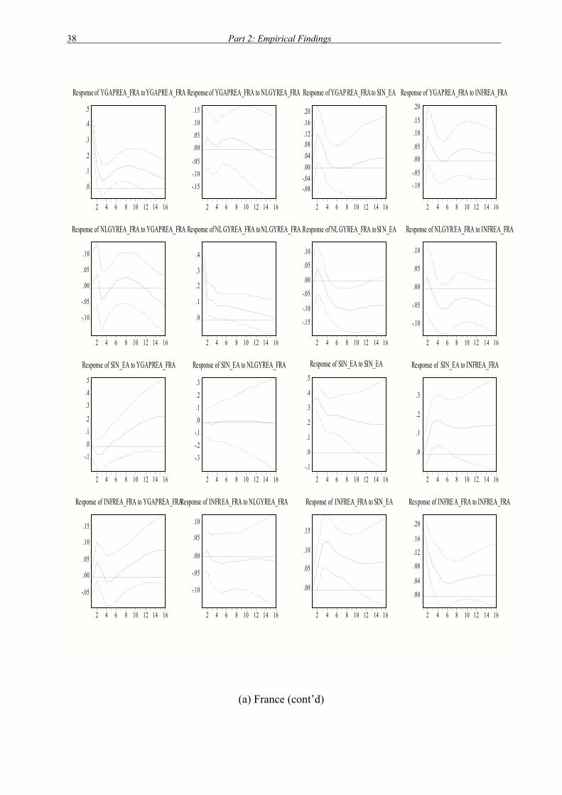
38 Part 2: Empirical Findings
(a) France (cont’d)
.0
.1
.2
.3
.4
.5
2 4 6 8 10 12 14 16
Response of YGAPREA_FRA to YGAPRE A_FRA
-.15-.10-.05
.00
.05
.10
.15
2 4 6 8 10 12 14 16
Response of YGAPREA_FRA to NLGYREA_FRA
-.08-.04.00.04.08.12.16.20
2 4 6 8 10 12 14 16
Response of YGAP REA_FRA to SIN_EA
-.10-.05
.00
.05
.10
.15
.20
2 4 6 8 10 12 14 16
Response of YGAPREA_FRA to INFREA_FRA
-.10
-.05
.00
.05
.10
2 4 6 8 10 12 14 16
Response of NLGYREA_FRA to YGAPREA_FRA
.0
.1
.2
.3
.4
2 4 6 8 10 12 14 16
Response of NL GYREA_FRA to NL GYREA_FRA
-.15
-.10
-.05
.00
.05
.10
2 4 6 8 10 12 14 16
Response of NL GYREA_FRA to SI N_EA
-.10
-.05
.00
.05
.10
2 4 6 8 10 12 14 16
Response of NLGYREA_FRA to INFREA_FRA
-.1.0.1.2
.3
.4
.5
2 4 6 8 10 12 14 16
Response of SIN_EA to YGAPREA_FRA
-.3-.2-.1.0.1.2.3
2 4 6 8 10 12 14 16
Response of SIN_EA to NLGYREA_FRA
-.1
.0
.1
.2
.3
.4
.5
2 4 6 8 10 12 14 16
Response of SIN_EA to SIN_EA
.0
.1
.2
.3
2 4 6 8 10 12 14 16
Response of SIN_EA to INFREA_FRA
-.05
.00
.05
.10
.15
2 4 6 8 10 12 14 16
Response of INFREA_FRA to YGAPREA_FRA
-.10
-.05
.00
.05
.10
2 4 6 8 10 12 14 16
Response of INFREA_FRA to NLGYREA_FRA
.00
.05
.10
.15
2 4 6 8 10 12 14 16
Response of INFREA_FRA to SIN_EA
.00
.04
.08
.12
.16
.20
2 4 6 8 10 12 14 16
Response of INFRE A_FRA to INFREA_FRA

Budgetary spillover and short-term interest rates 39
(b) Germany
-.2
.0
.2
.4
.6
2 4 6 8 10 12 14 16
Response of YGAP_GER to YGAPREA_GER
-.3-.2-.1.0.1.2.3.4
2 4 6 8 10 12 14 16
Response of YGAP_GER to NLGYREA_GER
-.2
.0
.2
.4
.6
.8
2 4 6 8 10 12 14 16
Response of YGAP_GER to SIN_EA
-.3-.2-.1.0.1.2.3.4.5
2 4 6 8 10 12 14 16
Response of YGAP_GER to INFREA_GER
.0
.1
.2
.3
.4
2 4 6 8 10 12 14 16
Response of NLGY_GER to YGAPREA_GER
-.3
-.2
-.1
.0
.1
2 4 6 8 10 12 14 16
Response of NLGY_GER to NLGYREA_GER
-.1
.0
.1
.2
.3
.4
2 4 6 8 10 12 14 16
Response of NLGY_GER to SIN_EA
-.2
-.1
.0
.1
2 4 6 8 10 12 14 16
Response of NLGY_GER to INFREA_GER
-.3
-.2
-.1.0
.1
.2
.3
2 4 6 8 10 12 14 16
Response of CUAY_GER to YGAPREA_GER
-.4-.3-.2-.1.0.1.2.3
2 4 6 8 10 12 14 16
Response of CUAY_GER to NLGYREA_GER
-.6
-.4
-.2
.0
.2
2 4 6 8 10 12 14 16
Response of CUAY_GER to SIN_EA
-.3-.2-.1.0.1.2.3.4
2 4 6 8 10 12 14 16
Response of CUAY_GER to INFREA_GER
.0
.1
.2
2 4 6 8 10 12 14 16
Response of INF_GER to YGAPREA_GER
-.2
-.1
.0
.1
2 4 6 8 10 12 14 16
Response of INF_GER to NLGYREA_GER
-.1
.0
.1
.2
.3
2 4 6 8 10 12 14 16
Response of INF_GER to SIN_EA
-.1
.0
.1
.2
2 4 6 8 10 12 14 16
Response of INF_GER to INFRE A_GER
Response to Generalized One S.D. Innovati ons ± 2 S.E.

40 Part 2: Empirical Findings
(b) Germany (cont’d)
-.1
.0
.1
.2
2 4 6 8 10 12 14 16
Response of YGAPREA_GER to YGAPREA_GER
-.10
-.05
.00
.05
.10
2 4 6 8 10 12 14 16
Response of YGAPREA_GER to NLGYREA_GER
-.2
-.1
.0
.1
2 4 6 8 10 12 14 16
Response of YGAPREA_GER to SIN_EA
-.20-.16-.12-.08-.04.00.04
2 4 6 8 10 12 14 16
Response of YGAPREA_GER to INFREA_GER
-.2
-.1
.0
.1
2 4 6 8 10 12 14 16
Response of NLGYREA_GER to YGAPREA_GER
.0
.1
.2
.3
2 4 6 8 10 12 14 16
Response of NLGYREA_GER to NLGYREA_GER
-.3
-.2
-.1
.0
2 4 6 8 10 12 14 16
Response of NLGYREA_GER to SIN_EA
-.20
-.15
-.10
-.05
.00
.05
2 4 6 8 10 12 14 16
Response of NLGYREA_GER to INFREA_GER
.0
.1
.2
.3
.4
.5
2 4 6 8 10 12 14 16
Response of SIN_EA to YGAPREA_GER
-.5-.4-.3-.2-.1.0.1.2
2 4 6 8 10 12 14 16
Response of SIN_EA to NLGYREA_GER
-.2-.1.0.1.2.3.4.5
2 4 6 8 10 12 14 16
Response of SIN_EA to SIN_EA
-.3-.2-.1.0.1.2.3
2 4 6 8 10 12 14 16
Response of SIN_E A to INFREA_GER
.00
.04
.08
.12
.16
2 4 6 8 10 12 14 16
Response of INFREA_GER to YGAPREA_GER
-.12
-.08
-.04
.00
.04
.08
2 4 6 8 10 12 14 16
Response of INFREA_GER to NLGYREA_GER
-.05
.00
.05
.10
.15
2 4 6 8 10 12 14 16
Response of INFREA_GER to SIN_EA
-.1
.0
.1
.2
2 4 6 8 10 12 14 16
Response of INFREA_GER to I NFRE A_GER

Budgetary spillover and short-term interest rates 41
(c) Italy
-.1
.0
.1
.2
.3
2 4 6 8 10 12 14 16
Response of YGAP_ITA to YGAPREA_ITA
-.1
.0
.1
.2
2 4 6 8 10 12 14 16
Response of YGAP_ITA to NLGYREA_ITA
-.2
-.1
.0
.1
.2
2 4 6 8 10 12 14 16
Response of YGAP_ITA to SIN_EA
-.2
-.1
.0
.1
.2
2 4 6 8 10 12 14 16
Response of YGAP_ITA to INFREA_ITA
-.4
-.3
-.2
-.1
.0
.1
2 4 6 8 10 12 14 16
Response of NLGY_ITA to YGAPREA_ITA
-.4
-.3
-.2
-.1
.0
.1
2 4 6 8 10 12 14 16
Response of NLGY_ITA to NLGYREA_ITA
-.3
-.2
-.1
.0
.1
.2
2 4 6 8 10 12 14 16
Response of NLGY_ITA to SIN_EA
-.2
-.1
.0
.1
.2
2 4 6 8 10 12 14 16
Response of NLGY_ITA to INFREA_ITA
-.3
-.2
-.1
.0
.1
2 4 6 8 10 12 14 16
Response of CUAY_ITA to YGAPREA_ITA
-.3
-.2
-.1
.0
.1
.2
2 4 6 8 10 12 14 16
Response of CUAY_ITA to NLGYREA_ITA
-.2
-.1
.0
.1
.2
2 4 6 8 10 12 14 16
Response of CUAY_ITA to SIN_EA
-.1
.0
.1
.2
2 4 6 8 10 12 14 16
Response of CUAY_ITA to INFREA_ITA
-.2-.1
.0
.1
.2
.3
.4
2 4 6 8 10 12 14 16
Response of INF_ITA to YGAPREA_ITA
-.3
-.2
-.1
.0
.1
.2
2 4 6 8 10 12 14 16
Response of INF_ITA to NLGYREA_ITA
-.2-.1.0.1.2.3.4
2 4 6 8 10 12 14 16
Response of INF_ITA to SIN_EA
-.1.0.1.2.3.4.5
2 4 6 8 10 12 14 16
Response of INF_ITA to INFREA_ITA
Response to Generalized One S.D. Innovations ± 2 S.E.

42 Part 2: Empirical Findings
(c) Italy (cont’d)
-.1.0.1.2.3.4.5.6
2 4 6 8 10 12 14 16
Response of YGAPREA_ITA to YGAPREA_ITA
-.05
.00
.05
.10
.15
.20
.25
2 4 6 8 10 12 14 16
Response of YGAPREA_ITA to NLGYREA_ITA
-.2
-.1
.0
.1
.2
2 4 6 8 10 12 14 16
Response of YGAPREA_ITA to SIN_EA
-.2
-.1
.0
.1
2 4 6 8 10 12 14 16
Response of YGAPREA_ITA to INFREA_ITA
-.05
.00
.05
.10
.15
.20
2 4 6 8 10 12 14 16
Response of NLGYREA_ITA to YGAPREA_ITA
.0
.1
.2
.3
.4
2 4 6 8 10 12 14 16
Response of NLGYREA_ITA to NLGYREA_ITA
-.10
-.05
.00
.05
.10
2 4 6 8 10 12 14 16
Response of NLGYREA_ITA to SIN_EA
-.16
-.12
-.08
-.04
.00
.04
2 4 6 8 10 12 14 16
Response of NLGYREA_ITA to INFREA_ITA
.0
.1
.2
.3
.4
2 4 6 8 10 12 14 16
Response of SIN_EA to YGAPREA_ITA
-.1
.0
.1
.2
.3
2 4 6 8 10 12 14 16
Response of SIN_EA to NLGYREA_ITA
-.2-.1.0.1.2.3.4.5
2 4 6 8 10 12 14 16
Response of SIN_EA to SIN_EA
-.1
.0
.1
.2
2 4 6 8 10 12 14 16
Response of SIN_EA to INFREA_ITA
-.10
-.05
.00
.05
.10
.15
.20
2 4 6 8 10 12 14 16
Response of INFREA_ITA to YGAPREA_ITA
-.10
-.05
.00
.05
.10
2 4 6 8 10 12 14 16
Response of INFREA_ITA to NLGYREA_ITA
-.08-.04.00.04.08.12.16.20
2 4 6 8 10 12 14 16
Response of INFREA_ITA to SIN_EA
.0
.1
.2
.3
2 4 6 8 10 12 14 16
Response of INFREA_ITA to INFREA_ITA

Budgetary spillover and short-term interest rates 43
Figure 4 (for the three largest euro area countries) and Figure 39 (for the smaller Member
States) provide a number of insights into the various spillover effects that have been identified
in chapter 2. In particular, we obtain (i) the spillover of a positive output shock in the rest of
the euro area on domestic output and domestic net exports (column 1). Next, we find (ii) the
spillover of an increase in inflation in the rest of the euro area on domestic inflation (column
4). Also, the effects of (iii) an increase in the fiscal balance in the rest of the euro area
(column 2) and (iv) an increase of the common short-term interest rate (column 3) on
domestic output, inflation and the fiscal balance can be assessed. The last four rows are of
minor importance, except for giving us the necessary information on the size and persistence
of the shocks (on the diagonal).
In the case of France, there is evidence of positive output and inflation spillover. The fiscal
balance is also positively affected by foreign output, fiscal shocks and inflation shocks.
Higher interest rates tend to reduce the fiscal balance, even though the effect is small. The
model of Germany finds positive spillover from the rest of the euro area on German output
and inflation. Higher interest rates tend to improve the German fiscal balance in the short run,
as if the German fiscal policy-makers were disciplined by higher interest rates. For Italy, we
find positive output and inflation spillover, together with fiscal spillover, suggesting that a
foreign fiscal consolidation improves output in Italy.
In the case of Austria, positive output and inflation spillover effects are present. Interest rate
shocks mainly affect inflation rather than output or the fiscal balance. Interestingly, a fiscal
balance shock in the rest of the euro area tends to induce changes in the same direction to the
Austrian fiscal balance. The model of Belgium is in many respects similar to the Austrian
case. Interestingly, however, the Belgian fiscal balance does not seem to react to deficits
elsewhere; it improves in the short-run in response to higher output in the rest of the euro
area, and it is negatively affected by interest rate increases. Most likely, this latter effect is
explained by a relatively high debt level over the sample period. Higher interest rates burden
the fiscal balance because of higher interest rate payments. Finland is outlying in the sense
that there is no evidence of positive output spillover from the rest of the euro area on Finnish
output. Compared with other countries, the evidence for spillover effects on the Finnish
economy from the rest of the euro area are weaker in practically all cases as suggests the
observation that the sign of the effects often changes over time and that the confidence bands
are rather large.

44 Part 2: Empirical Findings
Greece displays relatively small output, fiscal and interest rate spillover. The effect of
inflation spillover is relatively strong: inflation in the rest of the euro area seems to have a
substantial impact on Greek inflation as do short-term interest rates and output in the rest of
the euro area. The short-run improvement of Greek net exports after an inflation shock in the
rest of the euro area may reflect the improved competitiveness after such a shock as Greek
inflation is only gradually affected by the foreign inflation shock. Ireland is marked by
positive output and inflation spillover; the fiscal balance is negatively affected by an increase
in the short-term interest rate. The model of the Netherlands displays positive output spillover
but no inflation spillover. Interest rate increases tend to deteriorate the fiscal balance. These
results also hold in the case of Portugal. Moreover, the Portuguese results give some evidence
of fiscal spillover: an increase in the fiscal balance in the rest of the euro area tends to
increase output in Portugal, deteriorate its current account and increase inflation. In the case
of Spain, there is again evidence of positive output and inflation spillover. In addition, there is
evidence of a small negative effect from interest rates on output and the fiscal balance as well
as a positive effect from interest rate increases on net exports and inflation.
Summarising, in a number of cases restrictive fiscal policies in the rest of the euro area reduce
output in the domestic economy; in some cases there is hardly any effect or the effect is
positive. This is also the case for a restrictive monetary policy shock that raises the common
interest rate. Positive inflation and output shocks in the rest of the euro area also lead often to
higher inflation and output in the domestic economy. The evidence of these positive output
and inflation spillover effects is found to be relatively consistent and convincing.
Interestingly, there are not only important similarities but also considerable differences
between countries in terms of signs and sizes of the various spillover effects - note, moreover,
that for each Member State the same model structure (exogenous variables, lags of the VAR)
and practically the same sample period was used in the estimation, so that differences cannot
be due to these factors -. This suggests that there are strong heterogeneities between euro area
countries in the spillover, reflecting differences in economic structures, macroeconomic shock
characteristics and fiscal policy reactions. E.g. for the fiscal spillover many factors such as the
size and openness of a country, the size of the fiscal multipliers and the estimated persistence
of the fiscal shock may be important. The heterogeneities between countries suggest that
caution is needed when analysing the effects of shocks at the aggregate euro area level as in

Budgetary spillover and short-term interest rates 45
section 3.3 and extending the conclusions of the aggregate analysis to the individual Member
States.
In the model, external spillover is also present and measured by the impact of a depreciation
of the euro, the oil price and the US output on the output, fiscal balance, current account
balance and inflation in the euro area countries. It is assumed that for the individual countries
these variables are exogenous. In most cases an increase in the oil price tends to decrease
output, the current account balance and the fiscal balance and contribute to higher inflation. A
depreciation of the euro has in most countries a small positive effect on output and inflation.
In addition, in a significant number of countries output increases if US output increases.
Despite a few exceptions in detail, the general picture suggests that such external spillover on
individual euro area countries from oil price changes, changes in the euro exchange rate and
output outside the euro area (here represented by the US) is a source of spillover that does
matter also at the disaggregated level and, moreover, that countries vary to some degree in the
sign and size of this spillover.
A final aspect that needs to be addressed in this chapter concerns the spillover from shocks in
the three largest euro area countries on the rest of the euro area. The country VARs that were
estimated in (3.3) can also be used to analyse these spillover effects since they determine how
shocks in Germany, Italy and France affect the respective rest of the euro area. Figure 5
displays the spillover from output, the fiscal balance and inflation shocks in, respectively,
Germany, France and Italy on output (row 1), the fiscal balance (row 2), and inflation (row 4)
in the respective rest of the euro area. Also the effect on the short-run interest rate in the euro
area is shown (row 3).
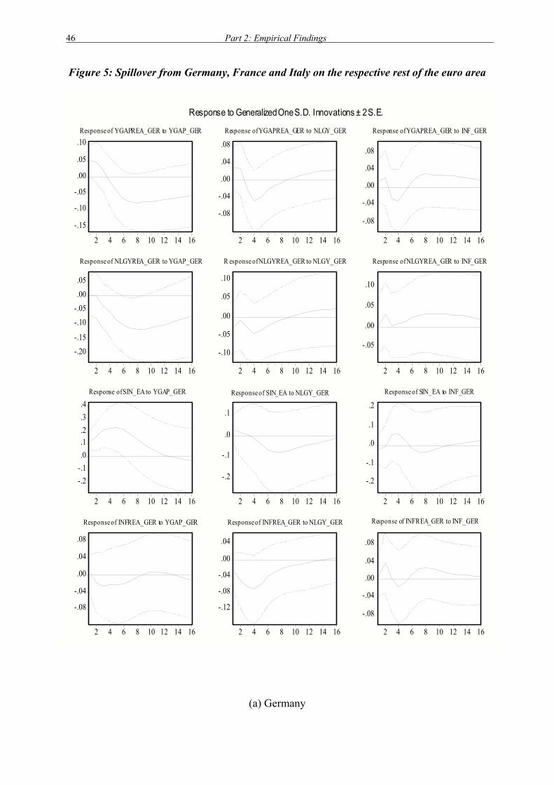
46 Part 2: Empirical Findings
Figure 5: Spillover from Germany, France and Italy on the respective rest of the euro area
(a) Germany
-.15
-.10
-.05
.00
.05
.10
2 4 6 8 10 12 14 16
Response of YGAPREA_GER to YGAP_GER
-.08
-.04
.00
.04
.08
2 4 6 8 10 12 14 16
Response of YGAPREA_GER to NLGY_GER
-.08
-.04
.00
.04
.08
2 4 6 8 10 12 14 16
Response of YGAPREA_GER to INF_GER
-.20-.15
-.10-.05.00.05
2 4 6 8 10 12 14 16
Response of NLGYREA_GER to YGAP_GER
-.10
-.05
.00
.05
.10
2 4 6 8 10 12 14 16
R esponse of NLGYREA_GER to NLGY_GER
-.05
.00
.05
.10
2 4 6 8 10 12 14 16
Response of NLGYREA_GER to INF_GER
-.2-.1.0.1.2.3.4
2 4 6 8 10 12 14 16
Response of SIN_EA to YGAP_GER
-.2
-.1
.0
.1
2 4 6 8 10 12 14 16
Response of SIN_EA to NLGY_GER
-.2
-.1
.0
.1
.2
2 4 6 8 10 12 14 16
Response of SIN_EA to INF_GER
-.08
-.04
.00
.04
.08
2 4 6 8 10 12 14 16
Response of INFREA_GER to YGAP_GER
-.12
-.08
-.04
.00
.04
2 4 6 8 10 12 14 16
Response of INFREA_GER to NLGY_GER
-.08
-.04
.00
.04
.08
2 4 6 8 10 12 14 16
Response of INFREA_GER to INF_GER
Response to Generalized One S.D. Innovations ± 2 S.E.

Budgetary spillover and short-term interest rates 47
(a) Germany (cont’d)
0.0
0.4
0.8
1.2
2 4 6 8 10 12 14 16
Response of YGAP_GER to YGAP_GER
-.4
-.2
.0
.2
.4
2 4 6 8 10 12 14 16
Response of YGAP_GER to NLGY_GER
-.8
-.6
-.4
-.2
.0
2 4 6 8 10 12 14 16
Response of YGAP_GER to INF_GER
-.1
.0
.1
.2
.3
.4
2 4 6 8 10 12 14 16
Response of NLGY_GER to YGAP_GER
.0
.2
.4
.6
.8
2 4 6 8 10 12 14 16
Response of NLGY_GER to NLGY_GER
-.3
-.2
-.1
.0
.1
.2
2 4 6 8 10 12 14 16
Response of NLGY_GER to INF_GER
-.8
-.6
-.4
-.2
.0
2 4 6 8 10 12 14 16
Response of CUAY_GER to YGAP_GER
-.5-.4-.3-.2-.1.0.1.2.3
2 4 6 8 10 12 14 16
Response of CUAY_GER to NLGY_GER
-.2
.0
.2
.4
.6
2 4 6 8 10 12 14 16
Response of CUAY_GER to INF_GER
-.3-.2-.1.0.1.2.3
2 4 6 8 10 12 14 16
Response of INF_GER to YGAP1_GER
-.12-.08-.04.00.04.08.12.16
2 4 6 8 10 12 14 16
Response of INF_GER to NLGY_GER
-.1.0.1.2.3.4.5.6
2 4 6 8 10 12 14 16
Response of INF_GER to INF_GER

48 Part 2: Empirical Findings
(b) France
-.1
.0
.1
.2
2 4 6 8 10 12 14 16
Response of YGAPREA_FRA to YGAP _FRA
-.1
.0
.1
.2
2 4 6 8 10 12 14 16
Response of YGAPREA_FRA to NLGY_FRA
.0
.1
.2
.3
.4
2 4 6 8 10 12 14 16
Response of YGAPREA_FRA to INF_FRA
-.2
-.1
.0
.1
.2
2 4 6 8 10 12 14 16
Response of NLGYREA_FRA to YGAP_FRA
-.1
.0
.1
.2
2 4 6 8 10 12 14 16
Response of NLGYREA_FRA to NLGY_FRA
-.3
-.2
-.1
.0
.1
2 4 6 8 10 12 14 16
Response of NLGYREA_FRA to INF_FRA
.0
.1
.2
.3
.4
.5
.6
2 4 6 8 10 12 14 16
Response of SIN_EA to YGAP_FRA
-.2-.1.0.1.2.3.4.5
2 4 6 8 10 12 14 16
Response of SIN_EA to NL GY_FRA
0.0
0.2
0.4
0.6
0.8
1.0
2 4 6 8 10 12 14 16
Response of SIN_EA to INF_FRA
.00
.05
.10
.15
.20
2 4 6 8 10 12 14 16
Response of INFREA_FRA to YGAP_FRA
-.08-.04.00.04.08.12.16
2 4 6 8 10 12 14 16
Response of I NFREA_FRA to NLGY_FRA
.0
.1
.2
.3
2 4 6 8 10 12 14 16
Response of INFREA_FRA to INF_FRA
Response to Generalized One S.D. Innovations ± 2 S.E.

Budgetary spillover and short-term interest rates 49
(b) France (cont’d)
-.1
.0
.1
.2
.3
.4
2 4 6 8 10 12 14 16
Response of YGAP_FRA to YGAP_FRA
-.2
-.1
.0
.1
.2
.3
.4
2 4 6 8 10 12 14 16
Response of YGAP_FRA to NLGY_FRA
.0
.1
.2
.3
.4
.5
.6
.7
2 4 6 8 10 12 14 16
Response of YGAP_FRA to INF_FRA
-.2
-.1
.0
.1
2 4 6 8 10 12 14 16
Response of NLGY_FRA to YGAP_FRA
-.2-.1.0.1.2.3.4
2 4 6 8 10 12 14 16
Response of NLGY_FRA to NLGY_FRA
-.2-.1.0.1.2.3.4.5.6
2 4 6 8 10 12 14 16
Response of NLGY_FRA to INF_FRA
-.3
-.2
-.1
.0
2 4 6 8 10 12 14 16
Response of CUAY_FRA to YGAP_FRA
-.2
-.1
.0
.1
.2
2 4 6 8 10 12 14 16
Response of CUAY_FRA to NLGY_FRA
-.5
-.4
-.3
-.2
-.1
.0
2 4 6 8 10 12 14 16
Response of CUAY_FRA to INF_FRA
-.2
-.1
.0
.1
.2
2 4 6 8 10 12 14 16
Response of INF_FRA to YGAP_FRA
-.2
-.1
.0
.1
.2
2 4 6 8 10 12 14 16
Response of INF_FRA to NLGY_FRA
-.1.0.1.2.3.4.5.6
2 4 6 8 10 12 14 16
Response of INF_FRA to INF_FRA

50 Part 2: Empirical Findings
(c) Italy
-.1
.0
.1
.2
.3
2 4 6 8 10 12 14 16
Response of YGAPREA_ITA to YGAP_ITA
- .2
- .1
.0
.1
2 4 6 8 10 12 14 16
Response of YGAPREA_ITA to NLGY_ITA
-.1
.0
.1
.2
.3
2 4 6 8 10 12 14 16
Response of YGAPREA_ITA to INF_ITA
- .05
.00
.05
.10
.15
2 4 6 8 10 12 14 16
Response of NLGYREA_ITA to YGAP_ITA
- .10
- .05
.00
.05
.10
2 4 6 8 10 12 14 16
Response of NLGYREA_ITA to NLGY_ITA
-.12-.08-.04.00.04.08.12.16
2 4 6 8 10 12 14 16
Response of NLGYREA_ITA to INF_ITA
.0
.1
.2
.3
.4
2 4 6 8 10 12 14 16
Response of SIN_EA to YGAP_ITA
- .3
- .2- .1
.0
.1
.2
2 4 6 8 10 12 14 16
Response of SIN_EA to NLGY_ITA
-.2-.1.0.1.2.3.4.5.6
2 4 6 8 10 12 14 16
Response of SIN_EA to INF_ITA
.00
.05
.10
.15
.20
.25
2 4 6 8 10 12 14 16
Response of INFREA_ITA to YGAP_ITA
- .15- .10- .05
.00
.05
.10
.15
2 4 6 8 10 12 14 16
Response of INFREA_ITA to NLG Y_ITA
.00
.04
.08
.12
.16
.20
.24
.28
2 4 6 8 10 12 14 16
Response of INFREA_ITA to INF_ITA
Response to Generalized One S.D. Innovations ± 2 S.E.

Budgetary spillover and short-term interest rates 51
(c) Italy (cont’d)
-.1.0.1.2.3.4.5.6
2 4 6 8 10 12 14 16
Response of YGAP_ITA to YGAP_ITA
- .3
- .2
- .1
.0
.1
.2
2 4 6 8 10 12 14 16
Response of YGAP_ITA to NLGY_ITA
-.2-.1.0.1.2.3.4
2 4 6 8 10 12 14 16
Response of YGAP_ITA to INF_ITA
-.5-.4-.3-.2-.1.0.1.2
2 4 6 8 10 12 14 16
Response of NLGY_ITA to YGAP_ITA
- .2
.0
.2
.4
.6
2 4 6 8 10 12 14 16
Response of NLGY_ITA to NLGY_ITA
-.6
-.4
-.2
.0
.2
2 4 6 8 10 12 14 16
Response of NLGY_ITA to INF_ITA
-.3
-.2
-.1
.0
.1
2 4 6 8 10 12 14 16
Response of CUAY_ITA to YGAP_ITA
- .1
.0
.1
.2
.3
2 4 6 8 10 12 14 16
Response of CUAY_ITA to NLGY_ITA
-.4-.3-.2-.1.0.1.2.3
2 4 6 8 10 12 14 16
Response of CUAY_ITA to INF_ITA
-.1.0.1.2.3.4.5.6.7
2 4 6 8 10 12 14 16
Response of INF_ITA to YGAP_ITA
- .4- .3- .2- .1.0.1.2.3
2 4 6 8 10 12 14 16
Response of INF_ITA to NLGY_ITA
.0
.2
.4
.6
.8
2 4 6 8 10 12 14 16
Response of INF_ITA to INF_ITA

52 Part 2: Empirical Findings
According to these estimations, the output and inflation spillover from shocks in France and
Italy to the rest of the euro area appear to be larger than those from Germany. We observe that
the spillover form France and Italy is often comparable and differ from the spillover produced
by German shocks in size and sometimes also in sign. That fiscal spillover from Germany is
rather small and/or counterintuitive may reflect statistical inaccuracies but also possibly
deeper phenomena. It is possible that German reunification and the subsequent fiscal
adjustments as well as the fundamental process of reforms and restructuring in the German
economy caused diverging developments in Germany as compared to the rest of the euro area
during the sample. The short-term interest rate in the euro area does not seem to be strongly
affected by individual fiscal balance shocks in Germany, France or Italy. This is in line with
the conclusion of the aggregate model where we also did not see a substantial effect of
aggregate fiscal shocks on interest rates.
3.5 Conclusions
In an integrated monetary and economic union such as the euro area, budgetary and other
types of spillover are likely to be important and complex. The short-run transmissions and
spillover of budgetary policy in the euro area are working through several different channels.
These include not only the traditional direct output and inflation spillover via net trade flows,
but also channels operating via the common interest rate (and monetary policy) and the euro
exchange rate.
The multitude of spillover and complex dynamics suggests that in particular a flexible
econometric approach like VAR models are useful if one is seeking to estimate spillover in
the euro area. In this chapter we have therefore estimated VAR models to analyse a number of
spillover effects that were considered important in the euro area.
First, the spillover at the level of the aggregate euro area was analysed. The effects of a
change in the euro area fiscal balance on output, net exports, interest rates, the euro exchange
rate and inflation in the euro area were estimated. In the aggregate model there is some -
albeit weak - evidence of direct spillover between monetary and fiscal policies in the euro
area. In particular, a positive interest rate shock reduces the fiscal balance. A positive shock to
the fiscal balance tends to reduce the interest rates in the short run, but this effect is rather
small and imprecisely estimated. Apart from this direct spillover, there are a number of
indirect connections between monetary and fiscal policies, running e.g. through output,

Budgetary spillover and short-term interest rates 53
inflation and depreciation of the euro. These indirect interdependencies were also analysed.
Finally, external factors - oil prices and US output – are another important source of spillover
on the aggregate euro area economy.
Second, the disaggregated analysis indicated that behind the aggregate analysis of the euro
area economy, there is a whole multitude of country-specific adjustments at work. The
analysis at the disaggregated level finds that the effects of fiscal policy in the euro area differ
substantially between countries. The most important results are: (i) there are positive direct
output and inflation spillover from the rest of the euro area on individual Member States.
(ii) The spillover from a fiscal policy shock in the rest of the euro area varies largely across
Member States. (iii) External shocks in the form of oil price changes, changes in the euro
exchange rate and fluctuations in the US output gap induce spillover to individual countries.
The timing and size of effects varies across countries. (iv) For the three large euro area
countries, Germany, France and Italy, spillover effects of fiscal policy on the rest of the euro
area were estimated. In this way, the effects of a fiscal shock in e.g. Germany on the rest of
the euro area were determined. Spillover from a fiscal shock in Germany on the rest of the
euro area seemed to be somewhat smaller than spillover from a fiscal shock in France or Italy,
but this result might be driven by significant changes not only to the economic structure but
also to fiscal polices in Germany after reunification.

54 Part 2: Empirical Findings
4 Budgetary spillover and long-term interest rates
4.1 Introduction
The effect of fiscal expansions on interest rates has commanded enormous theoretical interest,
and the hypothesis of crowding-out has received some – albeit not very robust – empirical
endorsement. Most economists would nevertheless agree with the position that consolidating
public finances reduces pressure on interest rates and will be conducive to economic growth
in the long run (Gale and Orszag, 2003). The crowding-out premise is also an important
motivation underlying the fiscal policy paradigm in EMU, as is evident from the policy
recommendations of both the European Commission and the ECB.
Capital flows between economically integrated economies tend to offset interest rate
differentials. Fiscal deficits don’t have necessarily to be financed by domestic financial
resources. The budgetary decision of one government may therefore affect the financing
conditions of other governments. This spillover effect is a purely pecuniary externality and
would not really command international coordination. Nevertheless, governments in open
economies that belong to a monetary union face different incentives. Basically, free riding
between independent fiscal authorities distorts the disciplinary incentives of higher interest
rates on governments and may therefore lead to excessive debt accumulation, and possibly
higher inflation (Beetsma and Bovenberg, 1999). Budget constraints indeed soften when the
fiscal relations between governments are not clearly spelled out. In EMU, the effects of debt
spillover have been contained with the no-bail out clause that is enshrined in Articles 101 and
103 of the Treaty of Nice, prohibiting overdraft facilities from the ECB or the assumption of
national commitments by other Member States. Keeping the national fiscal houses in order is
probably a sufficient condition to eliminate the distortion caused by free riding. The
numerical rules of the Stability and Growth Pact imply a debt target, and some reform
proposals on the Pact have argued for a stronger focus on debt consolidation. But the negative
coordination mechanism of deficit reduction should probably be conceived as pre-empting
fiscal bail outs.
There is little direct evidence for European countries on the crowding-out effects of
(accumulated) deficits, and there are even fewer studies that examine the spillover that fiscal
expansions has on long-term interest rates in a monetary union. The aim of this chapter is to
offer a framework to test both hypotheses. We do so by building on the literature that

Budgetary spillover and long-term interest rates 55
examines the effects of fiscal policy with small VAR models. That is, we examine the gross
effects that fiscal shocks have on domestic long-term interest rates. Accordingly, we specify a
VAR containing a simple economic model supplemented with rules-based fiscal policy and
long-term interest rates. We first examine this “national” SVAR for crowding-out for the
large euro area countries, a couple of smaller European countries and the euro area as a
whole. Then, we net out the spillover effects of public deficit and debt accumulation on a
country’s interest rate by benchmarking the model on aggregate euro area conditions.
The chapter is structured as follows. Section 4.2 makes the case for the modelling choice on
the basis of a critical literature review. The pros and cons of the specification and
identification of the SVAR model are detailed in section 4.3. The empirical results on gross
crowding-out effects of deficit accumulation follow in section 4.4, while section 4.5
investigates the spillover of fiscal policies. The final section 4.6 summarises the main results,
discusses some implications for the design of fiscal policy coordination in EMU, and closes
with some policy recommendations.
4.2 Deficits and interest rates: is there any robust evidence?
Many economists probably consider Ricardian Equivalence as a reasonable starting point for
the theoretical analysis of the effects of fiscal policy. Few would endorse it as a realistic
description of fiscal policy. The view that private savings do not fully offset the change in
public savings is not based on a firm empirical rejection of Ricardian Equivalence, for this
hypothesis is not directly testable. Plenty of empirical studies have therefore examined the
alternative question as to whether fiscal policy has any real economic effects. Recent evidence
seems to converge on at least some crowding-out effect of fiscal expansions on long-term
interest rates in practice. But no consensus has been reached: Elmendorf and Mankiw (1999)
even consider the results of the literature not informative.
Typically, interest rates are explained by including fiscal balances among the regressors in a
single equation – next to short-term interest rates, inflation and other relevant variables –
often in a panel framework. The specification usually derives from a partial equilibrium
“loanable funds” model in which the interest rate adjusts so as to maintain equality between
the supply and demand of bonds (Cebula, 1998). Alternative specifications are based on
intertemporal models of saving behaviour (Laubach, 2003). A large number of studies employ

56 Part 2: Empirical Findings
various definitions of government deficit or debt, interest rates, econometric approach and
data set. These studies can basically give support for any possible view on crowding-out.7
The factors that determine interest rates are plenty of course, and long-term structural factors
probably account for much more of the variation in interest rates. But a major reason for the
ambiguous effect is due to the static specification of the relation between deficits and interest
rates in these models. Government bonds are actually traded on financial markets that are
forward looking. The anticipation of upcoming deficits may therefore result in higher long-
term rates already now, as the direct crowding-out of short-term rates accumulates in long-
term rates via the expectations hypothesis. As a consequence, the exclusion of either of the
ends of the term structure could also bias the results (Bernheim, 1987). Expectations of higher
future deficits would show up directly in the slope of the yield curve, as future short-term
rates rise. Those studies that include expectations of future fiscal developments – for example,
by using the fiscal forecasts of the Congressional Budget Office (CBO) in the United States –
unanimously find significantly positive effects of expected deficits on expectations of interest
rate moves (Laubach, 2003).8 Some studies capture interest rate expectations by modelling
the effects on the entire term structure, and thereby obviate the need for modelling the
determinants of interest rates (Reinhart and Sack, 2000; Lindé, 2001 or Canzoneri et al.,
2002). Another way of capturing agents’ expectations is through the “news” approach to
public announcements of fiscal policy changes. Event studies try to detect the impact of
unexpected changes in fiscal policy on financial markets, much alike the narrative VAR
approach of Ramey and Shapiro (1998).9
Any direct relation between interest rates and fiscal balances is moreover obscured by
contemporaneous influences of countercyclical monetary policy, the workings of automatic
fiscal stabilisers and any economic effects of fiscal policy itself. In addition, the endogeneity
of the fiscal balance to interest rates, via the higher interest payments on outstanding debt
obligations, further cloud the direction of causality.10 For these reasons, the econometric
evidence of most reduced form empirical models remains rather inconclusive.
7 See the references in Barth et al. (1991), Gale and Orszag (2003) or the European Commission (2004). 8 The scarcity of such data for European countries prohibits a straightforward extension. The European Commission produces forecasts for year 2+t at most. 9 For the USA, Wachtel and Young (1987), Elmendorf (1996) and Kitchen (1996) give a good overview, while Knot (1996) or Afonso and Strauch (2003) give evidence for European countries.

Budgetary spillover and long-term interest rates 57
Such effects can only be uncovered in dynamic models. Large macroeconomic models can
account for the endogeneity of fiscal balances, but usually embed the consensus opinion of a
positive crowding-out effect of fiscal deficits on long-term interest rates already. VAR-
models have only recently received attention for the analysis of fiscal policy. Approaches that
identify fiscal shocks following the Blanchard and Perotti (2002) methodology, do not always
find significant effects.11 Some early applications that rely on Choleski orderings can be
found in Evans (1987a,b), Orr et al. (1995) or Miller and Russek (1996). Evans and Marshall
(2002), investigating the determinants of the variability in the nominal Treasury yield curve
with this method, do not find significant contributions of fiscal shocks. Tavares and Valkanov
(2001) on the other hand, find robust evidence for the impact of fiscal policy on bond returns,
relative to 3-month Treasury bills. Similarly, Canzoneri et al. (2002) include both the Federal
Funds rate and the 10 year bond yield in their structural VAR, and find significant and large
impact and long-term effects in response to spending shocks. A more recent application is
found in Ardagna et al. (2004), who find rather large crowding-out effects in a panel of
OECD countries, leading to cumulative 150 basis points rises at a horizon of 10 years.
The main hurdle in detecting changes in fiscal policy in VARs is that policy shocks need not
affect fiscal variables first. There are indeed anticipation effects as the implementation of
announced policy changes is subject to lengthy and visible political negotiations. Therefore, it
is hard to pin down all the information concerning future government actions the public has.
The unexpected component of changes in fiscal variables may bear little relation then to
projections of future fiscal policies. Elmendorf (1993) demonstrates the poor performance of
VAR-forecasts relative to fiscal projections. As the expected fiscal variables are merely
extrapolations from past data, they do not account sufficiently for newly available
information.
There may be a way around this problem by including the stock variable. Even if public debt
reflects past fiscal imbalances, it also constrains future budgetary policy actions. We may
indeed attribute the interpretation of a fiscal rule to the reaction of primary surpluses to public
debt, as in Bohn (1998). Deviations from sustainability in the past likely signal fiscal
corrections in the near to short-term future.12 In addition, public debt allows including
10 The use of fiscal projections or cyclically adjusted balances as in Cebula and Koch (1989) or Kitchen (2002) can remove these effects. 11 Note that in Blanchard and Perotti (2002) and consequent studies, only short-term interest rates are examined, as crowding-out is not the focus. 12 Moreover, if we interpret the higher interest rates following fiscal expansions as the higher rates the government has to offer investors to willingly hold more bonds, the interest rate becomes a direct – probably

58 Part 2: Empirical Findings
different degrees of persistence of fiscal deficits. Temporary changes that are expected to be
undone afterwards may have little impact, whereas the effects of permanent deficits that raise
debt permanently would crowd out interest rates considerably (Feldstein, 1986). There are
few studies that consider the indirect impact of deficits via debt accumulation. The direct
interest rate effect of debt is usually found to be small, or even negative (Ardagna et al.,
2004). There is also some evidence for non-linear effects: only at higher debt levels do
interest rates move significantly (O’Donovan et al., 1996; Conway and Orr, 2002)
Most of the empirical analysis pertains to US data, and this may provide few insights for EU
countries. In open economies that are economically integrated and do not impede trade or
financial flows, capital inflows may move massively so as to offset any domestic interest rate
rises following higher bond-financed deficits. In the limit of total capital mobility, these
increases are proportional to each country’s total indebtedness on the relevant market.
Yardstick comparisons across governments may partially offset this spillover, as debt
accumulation of one government increases the relative creditworthiness of comparable
governments. Empirical evidence on these spillover effects is little. Two different approaches
can be adopted. The spillover can be assessed directly from the effects of deficits and debt on
interest rates abroad. Alternatively, the effect of foreign capital inflows or fiscal developments
is netted out from the total domestic crowding-out effect. The reasoning is that the domestic
effect of fiscal expansions will likely be larger once these international linkages are controlled
for. In the reduced form approach, Cebula and Koch (1989) condition the relation between
interest rates and deficits on foreign capital inflows. Faini (2005) considers the fiscal effect on
interest rates at home and at EMU level contemporaneously. On a global scale, all spillover
effects should cancel out and a significant crowding-out effect restored. Tanzi and Lutz
(1993) look into the effects of domestic deficits and debt on global rates (see also Ford and
Laxton (1995)). Studies in the VAR-tradition have rather looked into the effect of domestic
fiscal policy changes on economic variables abroad. Ardagna et al. (2004) find significant
crowding-out effects from both domestic and average foreign fiscal expansions in a panel of
OECD countries. Beetsma and Giuliodori (2004) consider the impact of German fiscal policy
on the French and Italian economies, as does Marcellino (2002). In a further paper, Beetsma
et al. (2005) explicitly model the trade channel of fiscal spillover. Paesani et al. (2005) take a
somewhat different approach by identifying spillover from shocks to bond markets on
internationally linked capital markets. This allows the authors to consider also the direction of
non-linear – function of debt too. Evidence on default premia can be found in Alesina et al. (1992), Favero et al.

Budgetary spillover and long-term interest rates 59
the spillover: fiscal policy changes in the United States are argued to have a greater influence
on bond yields in Europe than vice versa. A similar argument is found in Brook (2003).
The spillover of domestic fiscal policies can only be enhanced if different governments
borrow in the same currency. In the absence of agreements specifying the fiscal relations
among governments, the crowding-out effect depends – ceteris paribus – on the aggregate
fiscal policy stance of all tiers of government. The free-riding problem between the various
tiers makes each fiscal authority disregard its intertemporal solvency constraint.13 A variety of
reasons may be invoked for the lack of credibility of no-bail out clauses that prevents other
governments (or the central bank) from saving the insolvent government.14 Political and
economic cohesion calls for fiscal solidarity. Systemic risk increases if government revenues
are interdependent: tax bases may be very mobile or elastic in highly synchronised and
integrated economies. Contagion effects may further amplify the debt accumulation spillover
when lenders interpret the difficulties of one debtor as signalling impending problems of
similar governments. The offsetting interest rate effects do not need to materialise then, as
default premia are spread out over the n members of the union. The distortion of the bond
market is one way to read a possible insignificant reaction of interest rates to debt
accumulation. Disentangling empirically the spillover effects that come from capital mobility
from those induced by monetary union is difficult. Landon and Smith (2000) compare the
significant cross-effects of federal and provincial debt in Canada. Beetsma and Giuliodori
(2004) simulate the effects of monetary union in their fiscal VAR for the three main euro area
economies. They find cross-country spillover from a fiscal expansion to be magnified via the
trade channel.
4.3 A stock-flow fiscal VAR for open economies
We propose using the VAR-approach to examine crowding-out of long-term interest rates
induced by changes in fiscal policy. We first set up the empirical model for inferring on
crowding-out in a closed economy, and then extend this model to indirectly infer on spillover
effects of fiscal policy. The central question of interest in the empirical analysis of the closed
economy is:
(1997) or Codogno et al. (2003). 13 We can refer to models of monetary union in both the Fiscal Theory of the Price Level (Canzoneri et al., 2001) and New-Keynesian settings (Beetsma and Jensen, 2002) for the complete economic effects of such free-riding behaviour. 14 See Bayoumi et al. (1995) for a discussion.

60 Part 2: Empirical Findings
QUESTION 1: What is the gross crowding-out effect of shocks to deficits – and the
accumulation of debt – on long-term interest rates within a country?
In other words, what is the overall crowding-out effect on domestic long-term interest rates
from fiscal expansions at home? To answer this question, we suggest specifying an empirical
model that contains the deficit flow and the stock of public debt. Attributing to the reaction of
deficits to debt the meaning of a systematic fiscal rule à la Bohn (1998) tackles the
anticipation problems discussed above. Rules have become an increasingly popular method of
describing policy behaviour, as well as a means of constraining discretionary policy
interventions. A positive reaction of the primary surplus to debt accumulation is considered a
necessary and sufficient condition for government solvency. Deviations from that rule likely
signal fiscal corrections in the near to short-term future.15 Consequently, this specification
overcomes inference problems on the anticipation of fiscal shocks.
The inclusion of debt moreover allows distinguishing the crowding-out effects of both deficits
and debt. Deficits typically are highly persistent. Permanent changes in deficits accrue in
public debt and may be argued to have stronger permanent effects on interest rates than
temporary reversals of cyclically induced deficits (Feldstein, 1986). We could thus label our
shock to debt as a “Permanent deficit” shock, and the shock to net lending as a “Temporary
deficit” shock. We can indeed discriminate both as we supplement the rules-based modelling
of the government sector with a small economic system, as in Favero (2003). Government
sets deficits in reaction to debt developments, but also as a function of the output gap and
inflation. This again helps identification, as the automatic stabilisers can be filtered from the
structural policy changes.
In order to account for the endogeneity problem of fiscal policy setting, the model is further
completed with inflation and output gap. The equations for inflation and output gap can then
be seen as summarising the economy in a very generic version of a Phillips curve, and an IS-
equation. We thus have a complete model of fiscal policy and the economic system to analyse
the effects on long-term interest rates. We consider principally the real long-term interest rate,
15 The inclusion of debt may cause inference problems on the VAR-parameters if there are non-linear effects of fiscal policy. While we later show that such different effects exist on interest rates, we show in Chapter 5 that no such switching effects happen on real economic variables for different levels of indebtedness.

Budgetary spillover and long-term interest rates 61
but also span the full term structure of interest rates by including the yield between both long
and short-term rates.16
To settle thoughts, the system can be divided in three blocks of variables: (a) the fiscal block
F that includes the debt tB and deficit td , [ ]'tt dBF = ; (b) the monetary block M that
includes some different specifications for interest rates, [ ]'tiM = ; and (c) the economic block
Y that summarises economic conditions in the output gap ty and inflation tp , [ ]'tt pyY = .
This specification can suffice for characterising effect of fiscal shocks in a closed economy.
The identification strategy that will be used in this chapter is based on a simple choleski
ordering, as in Beetsma and Giuliodori (2004) or Ardagna et al. (2004). There is no obvious
choice on placing debt before or after deficits. Debt is the accumulation of deficits over time,
and is arguably more endogenous than deficits. The initial conditions of debt can also be a
constraint on current fiscal actions. We therefore decide to put debt before the deficit so as to
allow for the strongest possible reaction of deficits for maintaining sustainability. We do not
take a position on the monetary block following the economic block or vice versa, but will
experiment with both possibilities. Placing the fiscal block first
(4.1a) [ ]'YMF or [ ]'MYF
implies no contemporaneous reaction of F to the economic variables, or to interest rates. The
reaction of the other variables is maximised though. But the reverse order
(4.1b) [ ]'FMY or [ ]'FYM
implies a complete crowding-out effect of government spending on GDP and interest rates.
Either of these assumptions is probably too extreme. The range between the most “liberal”
estimate of the effects of fiscal policy, and the most “conservative” estimate then gives an
indication on how robust our findings are. To that end, the impulse response functions of the
interest rate variable following upon a 1% fiscal deficit or debt to GDP shocks are
16The short-term rate is mainly influenced by day-to-day monetary policy decisions, and its reaction to fiscal imbalances has hardly ever been found significant. The long-term rate may capture inflation expectations, however. Mehra (2001) argues that by reacting precisely to inflation scares in these expectations, monetary policy can pre-empt inflationary bursts.

62 Part 2: Empirical Findings
summarised in a single graph for all four possible choleski orders. They are plotted over a 10-
year horizon, together with the maximum and averages of the four bootstrapped 90%
confidence intervals.17
The detection of crowding-out would be favourable for the no-bail out clause, as it succeeds
in separating different bond markets. A necessary condition for market discipline to work is
then fulfilled. A non-significant response on the other hand, might be consistent with no
interest effects of fiscal imbalances at all – in support of Ricardian equivalence. However, the
reaction still accrues the responses in a closed economy with any attenuating influences of
international capital flows and monetary union. A non-significant response could also be
consistent with strong spillover effects. We therefore model an open economy fiscal VAR to
net out the spillover of fiscal policy settings abroad on domestic long term rates. This answers
the second question of this chapter:
QUESTION 2: What is the net crowding-out effect of shocks to deficits – and the
accumulation of debt – on domestic long-term interest rates, in addition to the
spillover effect of other countries’ deficits and debt accumulation?
That is, is there any relevant crowding-out effect of deficit accumulation on a country’s long-
term interest rates, once the effects of foreign fiscal policies are accounted for? With the
simple VAR-models we propose, we just control the complete crowding-out effect for foreign
debt and interest rate spillover. We do not attempt to distinguish the spillover arising from
financial integration from those coming from the moral-hazard channel of no-bail out or
contagion effects. A significantly positive response to fiscal expansion at home is consistent
with the existence of each of these spillover effects. An insignificant crowding-out effect is
evidence for the Ricardian Equivalence proposition.18
To examine the second question, we adopt the same specification for the VAR, and consider
two strategies for modelling open economies. Empirical open economy models have to
struggle with the burden of over-parameterisation. Ideally, one would analyse the reciprocal
interest rate effects of changes in fiscal policies in both the home and foreign country
(Marcellino, 2002). The paucity of fiscal data for European countries renders this infeasible,
and we need to make some simplifying assumptions.
17 The VAR model always includes a constant and two lags of each endogenous variable.

Budgetary spillover and long-term interest rates 63
In first instance, we scale down the model by assuming identical transmission mechanisms in
all countries. We express all variables in country i as a difference to the same variable for the
euro area.19 This identifies asymmetric shocks across countries only. It expresses the idea that
only country-specific deviations from average economic and fiscal conditions in the euro area
matter for the effect of changes in fiscal policies on interest rates. We can write the model
concisely, as in (4.2a), for the various orderings of the fiscal, interest rate and economic bloc:
(4.2a) [ ]'*** YYMMFF −−− or [ ]'*** MMYYFF −−− or
[ ]'*** FFMMYY −−− or [ ]'*** FFYYMM −−−
We can then indirectly assess the importance of spillover from any stronger domestic
crowding-out effect. Note that the interpretation of the results differs from the “closed
economy” version. There, fiscal shocks lead to some percentage point change in interest rates.
In this model, fiscal shocks are relative to euro area fiscal developments, and have domestic
interest rate effects that are relative to euro area wide interest rate changes. We therefore
measure the relative change in interest rates. Also, shocks cannot be scaled to GDP and the
impulse responses follow upon a one standard deviation shock now.
In second instance, we adopt a small open economy assumption by adding the benchmark
euro area interest rate *i and/or public debt *B as exogenous variables to the VAR of country
i . That is, we control for the marginal effect on domestic fiscal policies. We take the
benchmark variables *i and/or *B as exogenous, but leave the order of the other variables
otherwise unchanged, as in (4.2b):
(4.2b) [ ]'|** YMFDi or [ ]'|** MYFDi or
[ ]'|** FMYDi or [ ]'|** FYMDi .
This benchmarking method loosens the restriction that all data enter in differences, but
becomes less realistic for larger economies.20 This interprets any variation in domestic interest
18 Only the yardstick comparison of relative debt levels would also mitigate crowding-out effects. 19 Where the own country’s contribution has been taken out. 20 Under an alternative assumption, a subset of countries could be analysed. This limits spillover and the role of common shocks (Prasad and Lumsdaine, 2003). One may also restrict the VAR coefficients for all countries. With heterogeneous fiscal stances, this may not be realistic.

64 Part 2: Empirical Findings
rates, for given conditions at the euro area level. In other words, it tells by how much
domestic rates would increase, given the rates at the euro area level.
Seen in combination with model (2a) this then allows inferring upon the importance of
spillover. If – for given euro area rates – fiscal shocks change the country spread (model 2b),
but do not lead to significant responses in relative interest rates following country-specific
fiscal shocks (model 2a), then this interest gap measures the attenuation of interest rates due
to spillover.
Data It suffices to look at the large number of studies, to see that various choices on the data
specification are possible. Limited availability of fiscal data constrains the choice of sample
and frequency. The data that we use in the empirical models mainly come from the annual
database of AMECO of the European Commission. This is the highest frequency at which a
standardised dataset covering fiscal data for EU countries over a maximum time span from
1960 to 2004 is available.21 The analysis focuses on the entire euro area, the largest EMU
economies (Germany, France and Italy) and a group of smaller ones (Austria, Belgium,
Finland and The Netherlands). We also consider the United Kingdom, for it provides a check
on the euro area results.
Regarding the deficit, we consider total net lending of the general government expressed as a
ratio to GDP for at least three reasons. 22 First, total net lending is of direct interest to fiscal
policy-makers. Second, the spurious relation that exists between the overall deficit and
interest rates is taken account of in the specification of the VAR. The reverse causality
problem of rising interest rates that induce compensation for higher interest payments on
outstanding debt is entirely included in our specification. Third, debt – which we take to be
the general government debt ratio to GDP – is arguably a more endogenous variable than the
primary deficit. The latter reacts to output and perhaps inflation, whereas debt and total
deficits are also influenced by interest rates. Placing debt before total deficits in (1a-b) thus is
less problematic then.
21 See Table 17 and Table 18 in Appendix 2c for details. 22 General government data consolidate across government levels, regardless the country-specific devolution of fiscal powers.

Budgetary spillover and long-term interest rates 65
The variables describing the economy are taken to be the CPI inflation rate, and the output
gap relative to potential GDP. As inflation is already included in the model as a separate
variable, the long-term interest rate on 10-year government bonds is deflated by realised CPI.
One might prefer using expectations of inflation in order to maintain consistency with the
term structure. Surveys or forecasts for inflation are not available at that horizon for European
countries. Ardagna et al. (2004) use trend inflation to approximate inflation expectations but
find little differences in results between nominal, real or expected long-term rates. We
therefore use the current realised rate.
For the open economy model, we also need to specify the benchmark data. We suppose the
offsetting spillover effects to come from intra-euro area capital flows only. This is a debatable
choice. First, there is some evidence for global linkages rather than regional spillover (Tanzi
and Lutz, 1993). Second, the fiscal framework of EMU pertains to both euro area and other
Member States of the EU. The Stability and Growth Pact and the no-bail out clause apply to
both groups. Nevertheless, the consequences of fiscal free riding carry more weight for those
countries that share the same currency. We therefore limit our attention to the spillover
internal to EMU. The benchmark open economy variable is a euro area aggregate. The data
for this artificial euro area economy come from both the AMECO and the quarterly ECB-EAS
database.23 A given country i cannot always be assumed small relative to EMU. The larger
the country, the smaller the difference with the euro area average will be. We therefore need
to correct the euro area aggregate. For net lending and public debt, we simply subtract country
i ’s series from the euro area aggregate, and scale it with the relevant output variable. The
other variables for the hypothetical EU-11 are obtained by subtracting series i and then
rescaling the GDP-weighted aggregate. Unfortunately, aggregate data are not always
available: data on French public debt before 1978 are simply absent. The aggregate public
debt has therefore been constructed from those countries that represent together two thirds of
euro area GDP.
23 End of period data have been used to construct yearly data.

66 Part 2: Empirical Findings
4.4 Crowding-out effects of fiscal policies
This section first discusses the results on the crowding-out effects in closed economies. We
then assess these effects for the entire EMU so as to prepare the ground for the discussion of
spillover between euro area countries.
Let us consider first the results of model (4.1a-b). For the various Choleski-orderings, Figure
6 summarises the effects of a 1% shock to the net lending and debt ratio. The gross effect of a
positive 1% shock to the deficit is to temporarily increase long-term interest rates by about 20
basis points in all countries, except Finland. This increase is insignificant, except for the
Netherlands, in the very first years after the expansion.24 The crowding-out effect is much
more relevant in the long run for a shock to the public debt ratio. Its size is nevertheless
generally smaller, and the reaction is only really significant in the more indebted countries as
Belgium, the Netherlands and Italy. When debt has clearly derailed, rates rise much more over
a longer horizon. This result is common to the literature. Ardagna et al. (2004) find large
effects on interest rates only in countries with above-average levels of debt.25 The contrast
between the larger – but insignificant – short run impact of deficits, and the smaller long run
impact of debt, is also consistent with evidence in the literature (Engen and Hubbard, 2004).
Our evidence rather supports the hypothesis of Feldstein (1986) that interest rates should
respond to the permanent creation of deficits that accumulate in higher debt in the long term,
and not to temporary changes in fiscal policies. Having included both deficit and debt
probably explains why we do not find the (counterintuitive) negative impact of debt on long-
term interest rates that other authors have documented. Ardagna et al. (2004) find a
cumulative reaction to shocks in (primary) deficits of up to 66 basis points, but owe the
decline in interest rates upon debt shocks to liquidity effects.
We do not really document a significant crowding-out effect domestically. But even if the
spillover between open economies within in the euro area is large, in a relatively
homogeneous and closed area as EMU these effects cancel out on aggregate. Any crowding-
out effects could become more evident again at the euro area level. To gain some sight on the
relevance of the spillover channels internal to EMU, question 1 can be reexamined for the
entire euro area. As can be seen in Figure 7, crowding-out effects on European interest rates
24 All results are also rather robust to the ordering of the variables in the VAR, as all responses follow the same pattern. 25 There is no evidence for different responses of real economic variables under different levels of indebtedness, as shown in chapter 5.

Budgetary spillover and long-term interest rates 67
do not become much more pronounced. The impulse responses to debt shocks in the same
domestic VAR model show a robust long-term rise in the interest rate. Its size is small,
however, and not always significant. Deficit shocks have a shorter run impact in the order of
20 basis points, but these results are hardly significant. Of course, we have assumed that the
offsetting effects come from intra-European capital flows only. Global spillover on
international financial markets may be more relevant. This result indicates that spillover may
rather be due to financial integration than to an incredible no-bail out clause per se.
What about the role of fiscal policy in explaining variability in interest rates?. Table 1.
displays the percentage contribution of deficit and debt shocks in explaining the variance of
the real long-term interest rate at various horizons (1, 5 and 10 years). The overall
contribution of fiscal policy is rather small, but gets larger at longer horizons. In the euro area
as a whole, only 7% is explained by deficits and public debt. This outcome is to a large extent
determined by German fiscal policy, whose contribution is also rather small. The picture for
other countries is less clear. There is no evidence for a larger driver of fiscal policy in highly
indebted countries. Similarly, there is no larger role for debt in these countries. Rather,
deficits may signal incipient problems in highly indebted countries, and therefore provoke a
stronger reaction in interest rates (see e.g. Italy) (Drudi and Prati, 2000).
4.5 Spillover effects of fiscal policies
We are now ready to look into the crowding-out effects in an open economy. By
concentrating on the deviation of fiscal and economic conditions from the euro area
benchmark, we may recover a significant domestic crowding-out effect, and indirectly infer
on the importance of the spillover. As we examine euro area aggregates, we do not consider
the United Kingdom anymore.
The results from expressing the data in differences to the base country, following model
(42a), are summarised in Figure 8. The crowding-out effect is more mitigated than the
response in the closed economy. Neither deficit nor debt shocks produce any significant
response. This result tells us that any deviation from the average fiscal conditions specific to
that country, does not affect the relative country spread. In other words, asymmetric fiscal
shocks do not translate in relative rises in financing conditions. Given that we detect some
small but significant crowding-out effect in closed economies, this would indicate rather
strong spillover effects of any fiscal shock onto the aggregate interest rates, and little to no

68 Part 2: Empirical Findings
effect on country-specific variables, a result reminiscent of Faini (2005). As differences to the
benchmark are taken, the forecast error variance decomposition attributes a somewhat larger
role to fiscal policy deviations in explaining long-term rates. Again, the contribution of
deficits is larger than the one of debt for the highly indebted countries (Table 2).
These results can give a false picture if asymmetric shocks do not play an important role.
Instead of imposing the restriction of variables entering in differences, we now consider the
small open economy assumption. As specified in (4.2b), we control for the euro area debt
ratio, euro area real long-term interest rates, or both, by adding these to the domestic model.
Figure 9, Figure 10 and Figure 11 display the results for this open economy SVAR.
Controlling for aggregate public debt seems to matter little: we nearly replicate the results of
the domestic model (4.1a-b) are basically confirmed. Debt shocks have large cumulative
effects on interest rates, but these are again significant in highly indebted countries only. A
more promising approach seems to benchmark the domestic interest rate to the corresponding
euro area rate. Table 3 sums up the graphical evidence from Figure 10 by setting out the point
estimate and the error bounds, as well as the peak effects, for a horizon of up to 5 years. There
is now a significant increase in the long-term rates in response to a 1% shock in the debt ratio.
The effect is also rather precisely estimated, and robust to the chosen choleski order. It can be
seen that this effect is again more pronounced for the highly indebted countries, but is also
much stronger for the other countries. The size of the effect is moreover sizeable. For most
countries, the peak effect is between 30 and 40 basis points, and is reached after 4 years. For
the highly indebted countries, this goes even up to 60 or 70 basis points, as for example in the
Netherlands and Belgium. Deficit shocks do not have significant effects. Only in Germany
and Austria is no crowding-out found back at all. This indiscernible effect may be explained
by the weight of Germany in the euro area. With a combination of euro area debt and interest
rates, the same results are obtained. Euro area debt adds little in explaining crowding-out
domestically. This again favours the hypothesis that capital market linkages are crucial for the
spillover of fiscal policies, rather than the fiscal framework.
Not surprisingly, debt contributes relatively more to explaining the variance of interest rates
when it is the only variable added to the domestic VAR (Table 4). When euro area interest
rates are incorporated, its contribution to the variance of the long-term rates is much smaller
than that of deficits. This holds even if the effects of net lending shocks are not relevant. It
rather supports the signalling effect of deficits for unsustainable longer-term fiscal policies.
Budgetary spillover and long-term interest rates 69
Overall, neither net lending nor public debt is an important determinant of real long-term
rates, and certainly not at short-term horizons.
The results for the United Kingdom also give an indirect answer as to whether spillover is
more relevant for EMU than EU. The open economy model is only slightly less successful for
the United Kingdom in finding significant effects of debt accumulation than in other
countries. There is nevertheless a change similar to other EU countries. A tentative conclusion
is that the spillover of financial integration is relatively more important than that related to
EMU.
How do we square the significant effect in the marginal open economy VAR with the
evidence for strong spillover effects in the first open economy model? In the first case, we
consider a relative fiscal shock that has a non-significant impact on relative spreads. If we
keep the benchmark interest rate fixed, there is, ceteris paribus, a large impact on the domestic
interest rate. This indicates that changes in the fiscal stance do not affect so much the country
spread, but rather affect the aggregate level of interest rates. This confirms the interpretation
in Faini (2005). Actually, the point estimates in Faini (2005) are very close to ours. A one
percent expansion in EMU primary balances raises the EMU rate on average by 41 basis
points in his study. Our country-specific results show such effects to lie between 30 and 70
basis points. The insignificant effect on relative spreads is also corroborated by the small 5
basis points rise in Faini (2005), or in studies that investigate default premia (Favero et al.,
1997; Codogno et al., 2003). Any consolidation that an individual country undertakes, will
thus largely spillover to euro area interest rates. The eventual gain for each country in terms of
lower interest rates is rather small, even for the highly indebted countries. A coordinated
action for bringing down debt ratios across the EU would pay off with substantially lower
long-term interest rates.
The results may be sensitive to the specification we have considered. A novelty we have
introduced is to make debt endogenous in the empirical model. In this case, the VAR equation
for debt describes the accumulation of deficits via past fiscal imbalances. Alternatively, debt
could be specified as an exogenous constraint on the economic model, reflecting initial fiscal
conditions. The VAR equation in the deficit can still be considered a fiscal rule then. This
model is examined in Appendix 2a. The main lesson is that imposing the stock of public debt
as a control variable insufficiently accounts for the persistence of deficits, and the

70 Part 2: Empirical Findings
accumulation of fiscal imbalances over time. There are hardly any significant responses to 1%
shocks in the net lending ratio, except in Belgium and the Netherlands. Modelling both debt
and deficits, and retrieving “Permanent deficit” from debt and “Temporary deficit” shocks
from net lending, helps in the identification.
Another robust check concerns the specification of the interest rate. We have chosen to
include a real long-term rate, but many studies consider the yield instead. Laubach (2003)
argues that taking into account both ends of the term structure may improve inference on
crowding-out effects. Ardagna et al. (2004) find little differences, however, for any of the
various measures of interest rates that they examine. We re-estimate all the specifications of
closed and open economy models by using the yield between long and short-term rates. The
results are summarised in Appendix 2b. There is a consistent swap of the impulse response
across all specifications, as is demonstrated in Figure 43. That is, debt accumulation causes
negative interest responses instead of positive ones, or weakens the significant response of
long-term rates. This result, also found in Ardagna et al. (2004), must be due to the stronger
responses of short-term rates, and can probably be explained by restrictive countercyclical
responses of monetary policy.26 Other results are relatively unaffected. There is also some
doubt on the stability of some of these specifications. By considering spreads, fundamental
determinants of interest rates are to a large extent cancelled out, and are affected more by
fiscal conditions. In this case, the deficit and debt shocks obviously explain more of the
variance in the yield. The results stand in contrast with specifications that include both short
and long-term rates separately. Both Tavares and Valkanov (2001) or Canzoneri et al. (2002)
find large and positive effects on market returns.
4.6 Summary and policy recommendations
The fiscal policy paradigm in EMU is strongly based on the crowding-out effect of fiscal
expansions on long-term interest rates. Fears of fiscal profligacy underlie the fiscal rules of
EMU, however. The mitigating effect of financial integration on domestic interest rates is
only enhanced by the expectations of fiscal or monetary bailouts under a common currency.
Such spillover effects would only exacerbate crowding-out effects at the EMU level, while
insufficiently disciplining fiscal policy in individual Member States.
26 An alternative explanation is given by Caporale and Williams (2002) that attribute it to a portfolio effect. Investors switch from bad quality debt issues to those of more creditworthy issuers, decreasing the yield even if total outstanding debt rises.

Budgetary spillover and long-term interest rates 71
This chapter first constructs an empirical model to examine crowding-out effects of deficit
and debt accumulation in individual EU countries and the entire euro area. The VAR
supplements rules-based fiscal policy with a simple economic model and interest rates. This
model is then modified for examining spillover effects between open economies.
The main result is that spillover masks the effects of fiscal policy on long-term interest rates.
With the exception of some highly indebted countries, there are hardly significant interest rate
responses to changes in domestic fiscal policies as such. Changes in the fiscal stance do not
affect so much relative country spreads, but rather spillover to aggregate euro area interest
rates. There is some indirect evidence that this spillover is not related to EMU as such, but
derives from financial markets. We deduce this from responses for the euro area as a whole
being only slightly stronger than for the individual Member States. Also, there is no obvious
difference in the interest rate responses in the United Kingdom.
The consequence is that a single country would not even benefit partially from consolidation
of its own public finances. The drop in domestic interest rates is insignificant. The interest
rate spread is only marginally affected, while the decline in interest rates is thinly spread out
over all euro area economies. Even for the highly indebted countries, the gain is rather small.
A coordinated action for bringing down debt ratios across the EU would pay off with overall
substantially lower long-term interest rates. Take for example a permanent 1% consolidation
of the total deficit. This brings down interest rates by about 30 basis points, and even more so
for highly indebted countries.
The results have some further implication for the design of fiscal rules. Evidence in this
chapter reveals that permanent deficits create stronger crowding-out effects than temporary
fiscal imbalances. Evidence for highly indebted countries is rather clear cut on the large
impact on long-term rates. Fiscal rules should focus on the long-term objective of sustainable
public finances. Nevertheless, there are considerable benefits from concerted action of fiscal
policymakers that goes beyond simply constraining fiscal discretion. Coordinated action
could avoid free-riding on consolidation efforts in other countries. The political and economic
costs of unilateral coordination may well be larger than the longer run benefits from lower
interest rates. Joint consolidation of public finances could bring about quicker the desired
beneficial economic effects.

72 Part 2: Empirical Findings
However, this is subject to four important caveats. First, coordination may be difficult to
achieve if the distribution of economic benefits is uneven. It is mainly the highly indebted
countries that would benefit from consolidation, even if the results show that the marginal
gain is negligible (about 10 basis points).27 Second, we find that spillover mainly comes from
global capital markets. The eventual lowering of interest rates may be smaller than our
estimates suggest. Nevertheless, it should not be underestimated that EMU is one of the large
players on global bond markets. Third, the argument for coordination is perhaps not so
convincing when spillover comes from capital markets. After all, the mitigating effect of
financial markets is a purely pecuniary externality that does not really require international
coordination. The allocation of savings to the public or private sector, at home or abroad, is
efficient. The ongoing integration of financial markets under EMU can only have increased
this spillover. Finally, the contribution of fiscal policy to long-term interest rates is rather
small, and we find this to be a robust result. Other drivers of interest rates seem more
important. This needs some closer examination. If spillover is mainly related to capital market
integration, one hypothesis is that fiscal policies probably have global rather than regional
effects. Results in Tanzi and Lutz (1993) and Ardagna et al. (2004) go in this direction too.
An extension of the results to incorporate the fiscal stance in other OECD countries,
especially the United States and Japan, could shed some light on this. The evidence on
crowding-out effects in the entire euro area does not run counter to such an interpretation, as
financial integration has deepened substantially in the EU. The benefits of coordinated
consolidation have probably become larger over time. Monetary union is indeed a complete
overhaul of the monetary and the fiscal policy regime, however. The incentives on
governments’ financing decisions have changed completely, and are regulated by a
combination of deficit rules and the no-bail out clause. Our estimates are probably a
conservative lower bound on the importance of spillover. Evidence in Faini (2005) points to
somewhat stronger spillover effects since 1999, albeit for the highly indebted countries only.
In order to extrapolate the evidence to EMU, we need to construct an empirical benchmark
that mimics the effect of monetary union. Uniform monetary policy settings could be
simulated as in Beetsma and Giuliodori (2004).
27 This reflect the difference in the decline in interest rates when highly indebted countries undertake a unilateral domestic consolidation (as in model 4.1a-b), as compared to the spread relative to the exogenous euro are rates (as in model 4.2b).

Budgetary spillover and long-term interest rates 73
Figure 6: Domestic economy, SVAR model (4.1a-b): impulse responses of real long-term interest rates to shocks of 1% of GDP in net lending and debt ratio
shock to net lending ratio shock to debt ratio
Austria
-80
-60
-40
-20
0
20
40
60
80
1 2 3 4 5 6 7 8 9 10
-3
-2
-1
0
1
2
3
4
1 2 3 4 5 6 7 8 9 10
Belgium
-20
-10
0
10
20
30
40
1 2 3 4 5 6 7 8 9 10
-2
-1
0
1
2
3
4
5
6
1 2 3 4 5 6 7 8 9 10
Germany
-50
-40
-30
-20
-10
0
10
20
30
40
50
60
1 2 3 4 5 6 7 8 9 10
-6
-4
-2
0
2
4
6
1 2 3 4 5 6 7 8 9 10
Finland
-80
-60
-40
-20
0
20
40
60
1 2 3 4 5 6 7 8 9 10
-6
-4
-2
0
2
4
6
8
10
12
14
1 2 3 4 5 6 7 8 9 10
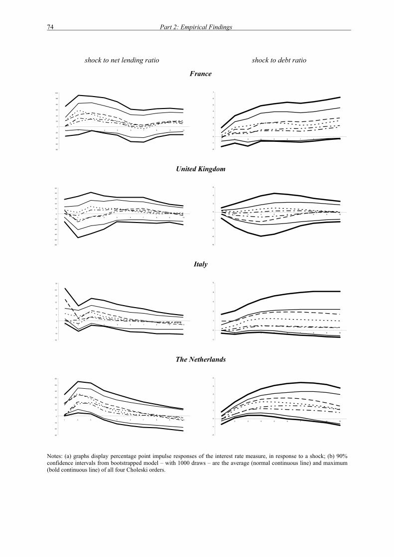
74 Part 2: Empirical Findings
shock to net lending ratio shock to debt ratio
France
-80
-60
-40
-20
0
20
40
60
80
100
120
1 2 3 4 5 6 7 8 9 10
-2
-1
0
1
2
3
4
5
6
7
1 2 3 4 5 6 7 8 9 10
United Kingdom
-60
-50
-40
-30
-20
-10
0
10
20
30
40
50
1 2 3 4 5 6 7 8 9 10
-8
-6
-4
-2
0
2
4
6
1 2 3 4 5 6 7 8 9 10
Italy
-15
-10
-5
0
5
10
15
20
25
30
1 2 3 4 5 6 7 8 9 10
-1
0
1
2
3
4
5
1 2 3 4 5 6 7 8 9 10
The Netherlands
-30
-20
-10
0
10
20
30
40
50
60
1 2 3 4 5 6 7 8 9 10
-2
-1
0
1
2
3
4
5
1 2 3 4 5 6 7 8 9 10
Notes: (a) graphs display percentage point impulse responses of the interest rate measure, in response to a shock; (b) 90% confidence intervals from bootstrapped model – with 1000 draws – are the average (normal continuous line) and maximum (bold continuous line) of all four Choleski orders.

Budgetary spillover and long-term interest rates 75
Figure 7: Euro area economy, SVAR model (4.1a-b): impulse responses of real long-term
interest rates to shocks of 1% of GDP in net lending and debt ratio
shock to net lending ratio shock to debt ratio
-0.3
-0.2
-0.1
0
0.1
0.2
0.3
0.4
0.5
0.6
1 2 3 4 5 6 7 8 9 10
-0.02
-0.01
0
0.01
0.02
0.03
0.04
0.05
1 2 3 4 5 6 7 8 9 10
Notes: (a) graphs display percentage impulse responses of the interest rate measure, in response to a shock; (b) 90% confidence intervals from bootstrapped model – with 1000 draws – are the average (normal continuous line) and maximum (bold continuous line) of all four Choleski orders.

76 Part 2: Empirical Findings
Figure 8: Open economy, SVAR model (4.2a): on difference of country i to euro area;
impulse responses of real long-term interest rates to standard deviation shocks in the net lending and debt ratio
shock to net lending ratio shock to debt ratio
Austria
-0.6
-0.4
-0.2
0
0.2
0.4
0.6
0.8
1
1 2 3 4 5 6 7 8 9 10
-1.2
-1
-0.8
-0.6
-0.4
-0.2
0
0.2
0.4
0.6
1 2 3 4 5 6 7 8 9 10
Belgium
-0.8
-0.6
-0.4
-0.2
0
0.2
0.4
0.6
1 2 3 4 5 6 7 8 9 10
-2
-1.5
-1
-0.5
0
0.5
1
1.5
2
1 2 3 4 5 6 7 8 9 10
Germany
-0.6
-0.4
-0.2
0
0.2
0.4
0.6
1 2 3 4 5 6 7 8 9 10
-1.5
-1
-0.5
0
0.5
1
1 2 3 4 5 6 7 8 9 10
Finland
-1 .2
-1
-0.8
-0.6
-0.4
-0.2
0
0.2
0.4
0.6
1 2 3 4 5 6 7 8 9 10
-1
-0.5
0
0.5
1
1.5
2
1 2 3 4 5 6 7 8 9 10
France
-0.8
-0.6
-0.4
-0.2
0
0.2
0.4
0.6
1 2 3 4 5 6 7 8 9 10
-1
-0.5
0
0.5
1
1.5
1 2 3 4 5 6 7 8 9 10

Budgetary spillover and long-term interest rates 77
shock to net lending ratio shock to debt ratio
Italy
-0.6
-0.5
-0.4
-0.3
-0.2
-0.1
0
0.1
0.2
0.3
0.4
1 2 3 4 5 6 7 8 9 10
-0.6
-0.4
-0.2
0
0.2
0.4
0.6
0.8
1
1.2
1.4
1 2 3 4 5 6 7 8 9 10
The Netherlands
-0.6
-0.4
-0.2
0
0.2
0.4
0.6
0.8
1 2 3 4 5 6 7 8 9 10
-1.5
-1
-0.5
0
0.5
1
1.5
2
1 2 3 4 5 6 7 8 9 10
Notes: (a) graphs display impulse responses of the interest rate measure, in response to a 1 standard deviation shock; (b) 90% confidence intervals from bootstrapped model – with 1000 draws – are the average (normal continuous line) and maximum (bold continuous line) of all four Choleski orders.

78 Part 2: Empirical Findings
Figure 9: Open economy, "marginal method", SVAR model (4.2b): conditioned on euro
area debt ratio; impulse responses of real long-term interest rates to shocks of 1% of GDP in net lending and debt ratio
shock to net lending ratio shock to debt ratio
Austria
-0.8
-0.6
-0.4
-0.2
0
0.2
0.4
0.6
1 2 3 4 5 6 7 8 9 10
-0.6
-0.4
-0.2
0
0.2
0.4
0.6
0.8
1
1 2 3 4 5 6 7 8 9 10
Belgium
-1 .2
-1
-0.8
-0.6
-0.4
-0.2
0
0.2
0.4
0.6
0.8
1
1 2 3 4 5 6 7 8 9 10
-1
-0.5
0
0.5
1
1.5
2
2.5
3
1 2 3 4 5 6 7 8 9 10
Germany
-0.6
-0.4
-0.2
0
0.2
0.4
0.6
1 2 3 4 5 6 7 8 9 10
-1.5
-1
-0.5
0
0.5
1
1 2 3 4 5 6 7 8 9 10
Finland
-1
-0.8
-0.6
-0.4
-0.2
0
0.2
0.4
0.6
1 2 3 4 5 6 7 8 9 10
-0.8
-0.6
-0.4
-0.2
0
0.2
0.4
0.6
0.8
1
1.2
1 2 3 4 5 6 7 8 9 10

Budgetary spillover and long-term interest rates 79
shock to net lending ratio shock to debt ratio
France
-0.6
-0.5
-0.4
-0.3
-0.2
-0.1
0
0.1
0.2
0.3
0.4
1 2 3 4 5 6 7 8 9 10
-0.6
-0.4
-0.2
0
0.2
0.4
0.6
0.8
1
1 2 3 4 5 6 7 8 9 10
Italy
-1
-0.8
-0.6
-0.4
-0.2
0
0.2
0.4
1 2 3 4 5 6 7 8 9 10
-0.4
-0.2
0
0.2
0.4
0.6
0.8
1
1.2
1.4
1 2 3 4 5 6 7 8 9 10
The Netherlands
-1
-0.8
-0.6
-0.4
-0.2
0
0.2
0.4
0.6
0.8
1 2 3 4 5 6 7 8 9 10
-1
-0.5
0
0.5
1
1.5
2
1 2 3 4 5 6 7 8 9 10
United Kingdom
-0.5
-0.4
-0.3
-0.2
-0.1
0
0.1
0.2
0.3
0.4
0.5
0.6
1 2 3 4 5 6 7 8 9 10
-1.4
-1.2
-1
-0.8
-0.6
-0.4
-0.2
0
0.2
0.4
0.6
0.8
1 2 3 4 5 6 7 8 9 10
Notes: (a) graphs display percentage impulse responses of the interest rate measure, in response to a shock; (b) 90% confidence intervals from bootstrapped model – with 1000 draws – are the average (normal continuous line) and maximum (bold continuous line) of all four Choleski orders.

80 Part 2: Empirical Findings
Figure 10: Open economy, "marginal method", SVAR model (4.2b): conditioned on euro
area real long-term interest rate; impulse responses of real long-term interest rates to shocks of 1% of GDP in net lending and debt ratio
shock to net lending ratio shock to debt ratio
Austria
-0.6
-0.4
-0.2
0
0.2
0.4
0.6
0.8
1 2 3 4 5 6 7 8 9 10
-0.8
-0.6
-0.4
-0.2
0
0.2
0.4
0.6
1 2 3 4 5 6 7 8 9 10
Belgium
-1
-0.8
-0.6
-0.4
-0.2
0
0.2
0.4
0.6
0.8
1 2 3 4 5 6 7 8 9 10
-1
-0.5
0
0.5
1
1.5
2
1 2 3 4 5 6 7 8 9 10
Germany
-0.5
-0.4
-0.3
-0.2
-0.1
0
0.1
0.2
0.3
0.4
0.5
1 2 3 4 5 6 7 8 9 10
-1.5
-1
-0.5
0
0.5
1
1 2 3 4 5 6 7 8 9 10
Finland
-0.8
-0.6
-0.4
-0.2
0
0.2
0.4
1 2 3 4 5 6 7 8 9 10
-0.8
-0.6
-0.4
-0.2
0
0.2
0.4
0.6
0.8
1
1 2 3 4 5 6 7 8 9 10

Budgetary spillover and long-term interest rates 81
shock to net lending ratio shock to debt ratio
France
-0.8
-0.6
-0.4
-0.2
0
0.2
0.4
0.6
1 2 3 4 5 6 7 8 9 10
-0.4
-0.2
0
0.2
0.4
0.6
0.8
1
1.2
1 2 3 4 5 6 7 8 9 10
Italy
-0.8
-0.6
-0.4
-0.2
0
0.2
0.4
1 2 3 4 5 6 7 8 9 10
-0.4
-0.2
0
0.2
0.4
0.6
0.8
1
1.2
1 2 3 4 5 6 7 8 9 10
The Netherlands
-0.8
-0.6
-0.4
-0.2
0
0.2
0.4
0.6
1 2 3 4 5 6 7 8 9 10
-0.8
-0.6
-0.4
-0.2
0
0.2
0.4
0.6
0.8
1
1.2
1.4
1 2 3 4 5 6 7 8 9 10
United Kingdom
-0.8
-0.6
-0.4
-0.2
0
0.2
0.4
0.6
1 2 3 4 5 6 7 8 9 10
-1
-0.5
0
0.5
1
1.5
2
1 2 3 4 5 6 7 8 9 10
Notes: (a) graphs display percentage impulse responses of the interest rate measure, in response to a shock; (b) 90% confidence intervals from bootstrapped model – with 1000 draws – are the average (normal continuous line) and maximum (bold continuous line) of all four Choleski orders.

82 Part 2: Empirical Findings
Figure 11: Open economy, "marginal method", SVAR model (4.2b): conditioned on euro area debt ratio and euro area real long-term interest rates; impulse responses of real long-
term interest rates to shocks of 1% of GDP in net lending and debt ratio
shock to net lending ratio shock to debt ratio Austria
-0.6
-0.4
-0.2
0
0.2
0.4
0.6
1 2 3 4 5 6 7 8 9 10
-0.6
-0.4
-0.2
0
0.2
0.4
0.6
1 2 3 4 5 6 7 8 9 10
Belgium
-1
-0.8
-0.6
-0.4
-0.2
0
0.2
0.4
0.6
1 2 3 4 5 6 7 8 9 10
-0.6
-0.4
-0.2
0
0.2
0.4
0.6
0.8
1
1.2
1.4
1.6
1 2 3 4 5 6 7 8 9 10
Germany
-0.5
-0.4
-0.3
-0.2
-0.1
0
0.1
0.2
0.3
0.4
0.5
1 2 3 4 5 6 7 8 9 10
-1.2
-1
-0.8
-0.6
-0.4
-0.2
0
0.2
0.4
0.6
0.8
1 2 3 4 5 6 7 8 9 10
Finland
-0.8
-0.6
-0.4
-0.2
0
0.2
0.4
0.6
1 2 3 4 5 6 7 8 9 10
-0.6
-0.4
-0.2
0
0.2
0.4
0.6
0.8
1 2 3 4 5 6 7 8 9 10

Budgetary spillover and long-term interest rates 83
shock to net lending ratio shock to debt ratio
France
-0.6
-0.5
-0.4
-0.3
-0.2
-0.1
0
0.1
0.2
0.3
0.4
0.5
1 2 3 4 5 6 7 8 9 10
-0.4
-0.3
-0.2
-0.1
0
0.1
0.2
0.3
0.4
0.5
0.6
0.7
1 2 3 4 5 6 7 8 9 10
Italy
-0.8
-0.6
-0.4
-0.2
0
0.2
0.4
1 2 3 4 5 6 7 8 9 10
-0.6
-0.4
-0.2
0
0.2
0.4
0.6
0.8
1
1 2 3 4 5 6 7 8 9 10
The Netherlands
-0.8
-0.6
-0.4
-0.2
0
0.2
0.4
0.6
1 2 3 4 5 6 7 8 9 10
-1
-0.5
0
0.5
1
1.5
1 2 3 4 5 6 7 8 9 10
United Kingdom
-0.6
-0.5
-0.4
-0.3
-0.2
-0.1
0
0.1
0.2
0.3
0.4
0.5
1 2 3 4 5 6 7 8 9 10
-0.8
-0.6
-0.4
-0.2
0
0.2
0.4
0.6
0.8
1
1.2
1.4
1 2 3 4 5 6 7 8 9 10
Notes: (a) graphs display percentage impulse responses of the interest rate measure, in response to a shock; (b) 90% confidence intervals from bootstrapped model – with 1000 draws – are the average (normal continuous line) and maximum (bold continuous line) of all four Choleski orders.
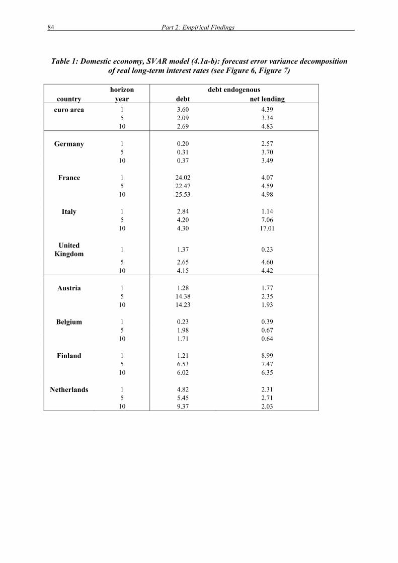
84 Part 2: Empirical Findings
Table 1: Domestic economy, SVAR model (4.1a-b): forecast error variance decomposition
of real long-term interest rates (see Figure 6, Figure 7)
horizon debt endogenous country year debt net lending
euro area 1 3.60 4.39 5 2.09 3.34 10 2.69 4.83
Germany 1 0.20 2.57 5 0.31 3.70 10 0.37 3.49
France 1 24.02 4.07 5 22.47 4.59 10 25.53 4.98
Italy 1 2.84 1.14 5 4.20 7.06 10 4.30 17.01
United Kingdom 1 1.37 0.23
5 2.65 4.60 10 4.15 4.42
Austria 1 1.28 1.77 5 14.38 2.35 10 14.23 1.93
Belgium 1 0.23 0.39 5 1.98 0.67 10 1.71 0.64
Finland 1 1.21 8.99 5 6.53 7.47 10 6.02 6.35
Netherlands 1 4.82 2.31 5 5.45 2.71 10 9.37 2.03

Budgetary spillover and long-term interest rates 85
Table 2: Open economy, SVAR model (4.2a): difference of country i to euro area; forecast
error variance decomposition of real long-term interest rates (see Figure 8)
horizon debt endogenous country year debt net lending
Germany 1 0.60 1.17 5 5.76 12.34 10 18.24 10.03
France 1 0.43 5.77 5 4.78 8.64 10 7.08 8.44
Italy 1 5.04 2.49 5 11.02 10.06 10 12.96 17.77
Austria 1 1.75 0.12 5 8.77 2.81 10 14.51 5.25
Belgium 1 0.01 0.03 5 3.72 7.65 10 6.93 7.11
Finland 1 0.06 0.15 5 1.25 7.37 10 1.34 8.20
Netherlands 1 1.63 10.97 5 0.93 4.50 10 2.50 3.90

86 Part 2: Empirical Findings
Table 3: Open economy, "marginal method": average point estimated response +/- 1.95
standard error bounds of impulse response to a 1% shock to the debt ratio (from Figure 10) horizon horizon Austria France
1 -0.15 -0.02 0.11 1 -0.12 0.05 0.21 2 -0.32 -0.06 0.20 2 -0.07 0.22 0.51 3 -0.53 -0.20 0.14 3 -0.08 0.27 0.62 4 -0.54 -0.19 0.17 4 -0.03 0.35 0.72 5 -0.42 -0.08 0.26 5 -0.06 0.32 0.71
Belgium Italy
1 -0.05 0.09 0.23 1 0.00 0.11 0.23 2 0.09 0.40 0.71 2 -0.11 0.19 0.48 3 0.22 0.65 1.08 3 -0.07 0.32 0.70 4 0.17 0.66 1.15 4 -0.05 0.38 0.80 5 0.09 0.60 1.10 5 -0.07 0.36 0.79
Germany The Netherlands
1 -0.05 0.08 0.21 1 -0.11 0.02 0.16 2 0.03 0.33 0.62 2 0.09 0.39 0.69 3 -0.34 0.04 0.42 3 0.15 0.54 0.92 4 -0.43 -0.04 0.35 4 0.13 0.57 1.01 5 -0.56 -0.12 0.31 5 0.02 0.49 0.95
Finland United Kingdom
1 -0.19 -0.06 0.06 1 -0.08 0.04 0.15 2 -0.18 0.13 0.45 2 -0.29 0.04 0.36 3 -0.20 0.26 0.73 3 -0.18 0.30 0.78 4 -0.26 0.28 0.83 4 -0.19 0.42 1.03 5 -0.39 0.17 0.73 5 -0.15 0.52 1.20
Notes: bold entries are point estimates; shaded cells indicate the peak effect.

Budgetary spillover and long-term interest rates 87
Table 4: Open economy, "marginal method", SVAR model (4.2b): forecast error variance
decomposition of real long-term interest rates (see Figure 9, Figure 10, Figure 11)
horizon
domestic debt endogenous; euro
area debt exogenous
domestic debt endogenous;
euro area real long-term rate
exogenous
domestic debt endogenous;
euro area debt and real long-term rate
exogenous
country year debt net lending debt net
lending debt net lending
Germany 1 0.01 1.32 3.78 5.74 0.59 2.54 5 0.41 3.34 4.41 10.55 2.08 8.02 10 0.37 3.29 4.52 9.96 2.01 7.52
France 1 24.72 5.09 16.30 0.00 7.72 7.37 5 23.47 4.80 14.40 7.11 5.76 35.26 10 25.98 4.66 13.94 8.71 5.15 31.04
Italy 1 3.77 1.95 0.75 0.57 1.11 0.40 5 3.30 15.05 1.27 1.25 6.20 2.85 10 15.67 10.24 1.43 1.53 13.11 2.34
United Kingdom 1 0.26 0.00 0.48 1.18 0.00 4.04
5 1.62 5.23 1.80 6.63 1.40 8.56 10 2.24 5.47 2.56 6.20 2.09 9.60
Austria 1 0.81 0.36 1.19 0.00 2.06 0.85 5 19.42 1.80 0.91 13.13 3.71 13.88 10 18.26 1.54 2.96 13.15 5.23 14.44
Belgium 1 0.81 0.12 0.33 3.42 0.00 0.89 5 2.78 1.55 0.37 7.96 0.76 2.40 10 1.94 1.63 0.56 8.37 1.56 2.43
Finland 1 0.40 13.53 0.04 8.82 0.64 7.75 5 10.84 23.73 8.46 9.84 11.34 8.30 10 24.19 12.57 7.51 11.48 11.41 10.02
Netherlands 1 6.75 3.84 5.68 2.57 6.71 2.67 5 10.34 6.62 8.00 3.24 9.19 3.80 10 16.46 5.22 7.45 4.20 8.05 4.77

88 Part 2: Empirical Findings
5 Budgetary stabilisation and the level of public debt
5.1 Introduction
In the previous chapters it is implicitly assumed that the relationship between the different
variables in the analysis is (close to) linear. This assumption is potentially controversial for
two key reasons. Firstly, the SVAR analysis used in the previous chapters may not perform
optimally in the presence of non-linearities. Secondly, the structural model used in the
remainder of this report is based on linear approximations of key macroeconomic
relationships.
In view of these concerns, this chapter provides a robustness check on the assumption of
linearity. It focuses on one potential source of non-linearity: the impact of a fiscal contraction
(expansion) and the initial level of public debt. If a relationship exists between these two
variables, then the impact of a change in government revenues or expenditure on the economy
(and, hence, through potential spillover effects on other economies) will vary from one
Member State to another.
The remainder of this chapter is divided into two parts. The first part presents an overview of
the literature on fiscal stabilisation and the level of public debt. The second empirically
examines whether the real effects of fiscal policy depend on the level of public debt.
5.2 A short overview of the literature
Traditional Keynesian thinking links a tighter fiscal policy to a reduced aggregate demand. If
a government raises taxes or cuts transfer payments, disposable income, and thereby also
private spending, is reduced. If a government decreases its consumption or investment,
aggregate demand is directly reduced. Multiplier-accelerator mechanisms will reinforce the
initial negative impact.
However, this basic Keynesian theory cannot explain why severe fiscal contractions in Ireland
and Denmark in the 1980s coincided with an economic boom (Giavazzi and Pagano, 1990).
Many potential explanations for these non-Keynesian effects were formulated, including
expectations, wealth and credibility effects, as well as crowding-out. In addition, the
macroeconomic effects of fiscal contractions depend on the composition (the impact of

Budgetary stabilisation and the level of public debt 89
raising taxes differs from that of cutting expenditures), the magnitude and the timing of a
fiscal contraction.
Furthermore, the debt level might be an important determinant of the outcome of a fiscal
consolidation. Firstly, a high debt level implies high future taxes. When debt increases, the tax
rate needed to stabilise the debt also increases. Blanchard (1990) postulates that taxes become
disruptive (in the sense that they reduce potential output) if they exceed a certain critical level,
known to the public28. Thus, the tax rate is a function of the debt level and a rise in this tax
rate is non-linear in its effects on output. He concludes that the higher the current tax rate, the
larger the potential output loss because of an excessive tax rate and the nearer the
‘catastrophe’ (i.e. a debt level close to the critical level) has come, the more a society has to
gain from a consolidation. In that “critical” context the effects of stabilising the debt will be
less negative than those predicted by Keynesian theory. To be able to predict the effects of a
fiscal policy action, it is important to know how much ‘fiscal space’ is left: i.e. how far away
the tax rate is from its critical level.
Secondly, a high debt level might also be a good predictor for the timing of the next
consolidation. Bertola and Drazen (1993) consider a government that gradually increases its
consumption until the government spending-to-GDP ratio reaches a critical level (the so-
called “trigger point”). At that point the government cuts drastically in its consumption. In
this model, the pre-stabilisation situation must deteriorate markedly to induce an inevitable
stabilisation. The closer “unsustainability” comes, the larger the probability of a fiscal
contraction in the next period becomes. When spending levels are already high, a further
unexpected increase raises the necessary expenditure cut even more, so the present discounted
value of future government expenditures (and future taxes) diminishes. As an agent bases his
consumption on expected future government spending, he will consume more. An increase in
government expenditures may be expansionary if people expect that expenditures will be cut
soon. By bringing the country on the edge of collapse, the prospects become less dark.
Note that in this set-up, agents react in a more Keynesian manner when the trigger point is
reached and more Ricardian when the debt situation is “as it should be”. However, when the
28 Dalamagas (1993) argues that in countries with a high debt-to-GDP ratio the public is less prone to suffer from some kind of debt-illusion. It will less likely consider government bonds to be net wealth, as they are more likely to be informed about the perverse consequences accompanying an expansionary fiscal policy. Journalists and the political opposition clearly have a motive to inform the public. In the model by Blanchard (1990) this could assure that the public will be capable to determine the critical level of taxation.

90 Part 2: Empirical Findings
trigger point is crossed and a consolidation does not occur, then a strong contraction of private
consumption will occur. People realise that they made an error in estimating future spending
(taxes) and they need to correct for it. An anticipated consolidation has no contractionary
effects. It is, however, difficult to imagine that consumers will spend more if a government
acts very profligate. This counter-intuitive result stems from the assumption that agents are
either infinitely lived or value their own well-being no more than that of future generations.
Sutherland (1995) assumes a more realistic approach. Agents are especially concerned about
the present. In normal times, i.e. when debt levels are moderate, consumers expect the next
budget consolidation to be far away. They do not adjust their expectation about future taxes in
response to a fiscal stimulus as the burden of such a consolidation will likely be put on the
next generations. So the current generation will react in a Keynesian way. However, when
debt levels are high (a critical level of government debt is reached), every new fiscal
expansion brings a consolidation alarmingly near. The “bill” is then likely to be presented
while the current generation is still alive. So they will have to carry the burden themselves. As
the cost of a fiscal consolidation outweighs numerous times the gain from the expansion, any
additional expansion will cause a contraction. So the link between current fiscal policy and
future expected taxes and the distribution of these expected future taxes across generations
will determine whether a fiscal policy is expansionary or contractionary. In this model, agents
react in a Keynesian manner under “normal circumstances” and in a non-Keynesian29 manner
in “crisis situations”.
Perotti (1999) integrates different aspects of these previous models. He looks at the share of
credit constrained people in a society30. For those people an unanticipated increase in taxes
will always lower their consumption, and a positive shock to government expenditures will
always increase it. Their consumption is completely determined by disposable income. Hence,
they resemble the agents in the Sutherland model. On the other hand, agents who are not
credit constrained will not always decrease consumption after an unexpected increase in taxes.
If government spending has not changed, the increase in current taxes will be exactly equal to
the drop in the present discounted value of expected future taxes (so consumption will not be
29 But also in a non-Ricardian manner. People will actually reduce their expenditures by a larger amount than the government increases its expenditures. 30 Afonso (2001) shows with a theoretical model that the bigger the proportion of non-rationed consumers, the more likely non-Keynesian effects will occur. The existence of non-Keynesian effects will also be more likely when interest rates are more responsive to changes in public revenues.

Budgetary stabilisation and the level of public debt 91
altered). These agents act in accordance with the Bertola and Drazen model. Finally, Perotti
incorporates the Blanchard model. By raising current taxes, current distorting effects of
taxation are strengthened. On the other hand, as future taxes are reduced, future distortions
form taxation also decrease. The net effect of these two opposite movements will determine
the impact on the unconstrained agents’ consumption. An unexpected increase in government
consumption will always depress private consumption as the present discounted value of
future taxes increases.
The combined effects of credit constrained and unconstrained agents determines the total
effect on private consumption. According to Perotti (1999) the sign of the total effect switches
at higher levels of government debt. An expenditure shock will be positive if (1) the debt
level is still low, (2) the probability that the same government will still be in office is large
and (3) the group of credit constrained people in the society is ‘large enough’. A low level of
debt also means a low level of future taxes, so slightly higher future taxes will still not be too
distorting. If the same government stays in office, taxes are likely to be lower than if a new
government is installed (as new preferences and priorities also lead to new expenditures).
These two factors limit the negative response of unconstrained agents’ consumption on a
fiscal expansion. Hence, the extra consumption by credit constrained people will keep the
upper hand. The percentage of credit constrained agents is crucial in this model. Their
increased (decreased) liquidity will produce a Keynesian outcome in case of an expansion
(contraction). Only if the ‘counter-reaction’ of unconstrained people is vigorous, the results
will be non-Keynesian.
To summarise: economic theory suggests that the effects of fiscal policy actions on economic
activity are influenced by the level of public debt. The nature of the relationship is dependent
on the degree of “Ricardianism” in economic life. However, since it is safe to assume that
agents discount the well-being of future generations and it is well known that market
imperfections exist, one expects that the effects of fiscal policy will be more Keynesian in low
debt times. Non-Keynesian effects are more likely in high debt episodes.
Although theory assigns an important role to the initial conditions, strong empirical evidence
confirming this notion has yet to be provided. Zaghini (1999) notes that in the recent
European experience, the level of debt before successful consolidations was on average twice
as high as before unsuccessful ones. Alesina and Ardagna (1998) and Ardagna (1999) detect

92 Part 2: Empirical Findings
only a weak (small and statistically insignificant) link between the lagged debt-to-GDP ratio
and the probability of a successful consolidation in OECD countries. Heylen and Everaert
(2000) reach the same conclusion.
The above studies cannot really verify or falsify the theoretical models, as they define neither
the critical debt level nor the available fiscal space. Theory only predicts that there will be
some kind of regime shift when a certain amount of debt accumulation is reached. The reason
for the difficulty in finding the importance of the debt level for the effects of fiscal policy may
be given by the fact that there are too few observations of these ‘critical debt situations’
within the sample. One has to face a difficult but essential question: from what level on can
the debt level be considered as being problematic?
In recent work, different possibilities were explored:
(i) Perotti (1999) uses the sum of the present discounted value of future government
expenditure and the cyclically adjusted government debt. If the observed value is
above the ninetieth percentile of the distribution of the sample, the situation is labelled
as problematic.
(ii) A second indicator proposed by Perotti (1999) is based on the budget deficit. If the
cyclically adjusted deficit as a share of trend GDP has exceeded a certain value in the
two previous years, a government is said to be in fiscal distress.
(iii) Gobbin and van Aarle (2001) use an indicator based on the Domar conditions on fiscal
sustainability. This indicator shows whether economic growth, interest rates, primary
deficit and government debt are consistent with achieving a ‘steady state level’ of
debt.
(iv) Gobbin and van Aarle (2001) derive an indicator from the Maastricht-criteria
concerning fiscal convergence. If a country does not comply with one of these two
criteria, it is said to be in fiscal distress.
All of the above indicators make sense, but they are not without criticism. The first three
indicators just shift the problem: one still has to choose, respectively, the percentile, an
acceptable value for the deficit or the correct steady state debt level. The fourth criterion is
more objective. Countries that did not satisfy the Maastricht-criteria could not join the EMU.
So stakes were high. However, it is only applicable to a limited number of countries (EU),
and only for a short period in time.

Budgetary stabilisation and the level of public debt 93
The empirical set-up of the papers by Perotti (1999) and Gobbin and van Aarle (2001) is
similar: in both contributions a consumption function specification is estimated, in which
fiscal variables interact with a dummy for fiscal distress. Perotti (1999) finds support for the
different effects of government spending in good times and in bad times (but not for taxation).
The results of Gobbin and van Aarle (2001) do not confirm this finding.
Höppner and Wesche (2000) use a Markov-switching approach to determine non-
conventional fiscal periods in Germany. They can identify two distinct regimes: one in which
the effects of fiscal policy are Keynesian and one in which they are rather non-Keynesian.
However, the shift between the regimes cannot be explained by a rise in the debt level or a
consolidation programme. If the debt situation worsens, the probability of remaining in the
Keynesian regime even increases.
5.3 The importance of the debt level: an empirical contribution
In this empirical contribution, we focus on the impact of the initial debt level on the outcome
of fiscal policy actions. Recently, it has been noted that the effects of fiscal policy actions can
differ across countries (Hogan, 2004). However, using individual countries is not a viable
solution since it strongly reduces the variability in the debt rate data. Therefore, we test for
non-linearities in a panel of EMU countries. By doing so, we implicitly impose a homogenous
impact of fiscal policies in those countries. This choice resembles the estimates in the
previous chapters in which we looked for the effects of the aggregate euro area economy on
the individual Member States.
Data
We use data from the ‘OECD economic outlook quarterly’ data set, with the exception of
inflation which was derived from the ‘OECD main economic indicators’ data set. In a
quarterly panel we include Finland, France, Ireland, Italy and the Netherlands. For most
countries we have data series from the first quarter of 1970 up to the first quarter of 2005.
Unfortunately, the available data do not allow the inclusion of (among others) Germany in
this analysis. To obtain a sample that is more representative for the entire euro area, we use
annual instead of quarterly data in the second part of this empirical contribution. It is also
commonly known that the quality of annual fiscal data is higher than that of quarterly data. In
this yearly panel Greece, Luxembourg and Portugal are excluded due to data limitations.

94 Part 2: Empirical Findings
Methodology
If the debt level determines the impact of fiscal policy on private consumption (or
investment), consumption (investment) functions will not be identical across countries.
Because we have no a priori knowledge as to how the coefficients of the fiscal policy
variables vary with the level of debt, we apply the endogenous threshold estimation technique
developed by Hansen (1997, 1999, 2000). The literature survey shows that previous work
suffers from the arbitrariness of the definition of the critical debt level. This is especially
problematic since the results are not robust to marginal changes of this definition. We avoid
this problem by determining the threshold debt level endogenously. The main problem is that,
since the threshold is unknown, it has to be estimated, meaning that the standard econometric
theory of estimation and inference is not valid. We estimate a consumption function of the
following form:
(5.1) 0 1 1 2 3 1 4 5 1 1'( .) ' ( .) '
t t t t t t t
LD t HD t t
C r r Y Y C FI F I Fdebt crit debt critα α α α α α β
εγ γ− − − −Δ = + + Δ + + Δ + +
+ Δ + Δ +< > ,
in which C denotes private consumption, r the real long-term interest rate, and Y disposable
household income. F is a vector containing all fiscal policy variables (all variables are in real
terms). I is and indicator function that depends on the debt level. The coefficients of the
changes in the fiscal variables (the γ-vector) depend on the debt level. The subscript ‘LD’
(‘HD’) refers to a debt level below (above) the critical one.
Given the near-consensus in the literature that the composition of fiscal policy matters for its
outcome, we do not use the budget deficit as a proxy for the fiscal stance. Instead, we
introduce different components of the budget. On the expenditure side we include government
investment (INV) and the sum of government consumption, subsidies and current transfers
(EXP). On the revenue side we use the sum of direct and indirect taxes (REV).
In addition to consumption, investment is also an important part of economic activity. If we
want to capture the impact of fiscal policy actions on the total economy, we need to broaden
the scope of the analysis. The specification of the investment function is similar to the one of
the consumption function (replacing consumption by investment). However, we attach more
weight to the estimates of the consumption function as the specification of the investment

Budgetary stabilisation and the level of public debt 95
function might be too elementary to really account for the complexity of investment
behaviour.
The threshold estimation technique jointly estimates the coefficients and the threshold level. It
selects the value of the threshold that minimises the sum of squared errors of the equation. It
is important to note that this does not mean that one cannot get significant results based on an
alternative value of the threshold variable. But if one believes that the coefficients on the
fiscal variables change once a certain level of debt is reached, then the threshold estimate is
the most likely suspect for the turning point given the available data. By means of
bootstrapping techniques we next determine whether the threshold effect is significant (see
Hansen, 1997, 1999, 2000).
Results
We construct a quarterly euro area panel that includes Italy, Finland, France, the Netherlands
and Ireland. Unfortunately, we lack data for Germany. Still the panel has some interesting
features: it comprises two large economies (France and Italy), it includes a country with an
interesting fiscal past (Ireland), and the debt rate has a wide range: from 8% to 135% of GDP.
We do not allow for a value of the threshold below 35% or above 95%. Doing so would imply
that the coefficient estimates for the smallest category would be based on less than 10% of the
data points (i.e. less than 55 observations). These results would not be sufficiently robust to
the presence of outliers. Note that for the highest debt levels almost all observations above the
debt threshold are found in only two countries, Italy and Ireland.
Our consumption (investment) function specification includes a lagged endogenous variable,
which means that fixed effects panel estimators could be biased and inconsistent
(Nickell, 1981). However, Judson and Owen (1999) show that this bias is small if the cross-
section dimension is small in relation to the time dimension of the panel. This is clearly the
case for our euro area panel, which covers only 5 countries and at least 81 quarters. A
comparison (not shown) of the GMM-estimates with the fixed effects estimates of the
consumption function without thresholds confirms that the results are very similar. Hence, we
continue to use the fixed effects estimation method.

96 Part 2: Empirical Findings
Below, we present two figures plotting the estimated coefficients of, respectively, changes in
government revenues and expenditure for different values of the threshold variable. The best
estimates are obtained for a debt ratio of about 90% (which means that in 131 episodes the
debt ratio is above the threshold).
From Figure 12 it is clear that the effect of revenue changes on private consumption does not
differ a lot between high debt and low debt times. Only near the upper bound (from a debt
ratio of 80% onwards) there seems to be a slight indication of non-Keynesian effects: the
impact of taxes on consumption first becomes less negative, then it is no longer significant.
Recall that the situation in Italy, and to a lesser extent in Ireland, will largely determine this
result.
Figure 12: Quarterly EMU panel: the impact of tax changes on private consumption
-0,07
-0,06
-0,05
-0,04
-0,03
-0,02
-0,01
035 40 45 50 55 60 65 70 75 80 85 90 95
REVlowREVhighREVhigh
Note: X-axis: debt rate that is used as threshold level Y-axis: coefficient of a change in government revenues in the consumption function “REVlow”: estimate below the threshold
“REVhigh”: estimate above the threshold Black marks indicate significant coefficients, hollow marks indicate insignificant coefficients.
The impact of changes in government spending on private consumption (Figure 13) is more in
line with the literature on non-Keynesian effects. For low debt levels the impact is similar
above and below the threshold. However, for higher debt levels, the impact of government
spending on private consumption is much smaller above than below the threshold. The effects
of government investment on private consumption display a pattern similar to the one of

Budgetary stabilisation and the level of public debt 97
taxes: the effects above and below the threshold are almost identical (but the estimated
coefficient above the threshold is insignificant in many cases).
Figure 13: Quarterly EMU panel: the impact of spending changes on private consumption
0
0,2
0,4
0,6
0,8
1
1,2
35 40 45 50 55 60 65 70 75 80 85 90 95
EXPlowEXPhigh
Note: X-axis: debt rate that is used as threshold level Y-axis: coefficient of a change in government spending in the consumption function “EXPlow”: estimate below the threshold
“EXPhigh”: estimate above the threshold.
Next, we construct a yearly panel of euro area countries. Moving from quarterly to yearly data
allows us to include more countries in the data set. We can expand the cross-section
dimension of the panel (to the detriment of the time dimension). The new panel consists of 9
countries: Austria, Belgium, Finland, France, Germany, Ireland, Italy, the Netherlands and
Spain. We cover the period 1977 to 2004. In the yearly panel the best estimates are obtained
for a debt ratio of 50% of GDP. We obtain similar (significant) results for the impact of tax
changes in times of low and high debt ratios.

98 Part 2: Empirical Findings
Figure 14: Yearly EMU panel: the impact of spending changes on private consumption
-0,15
-0,1
-0,05
0
0,05
0,1
45 50 55 60 65 70 75 80 85 90 95EXPlowEXPhighEXPlowEXPhigh
Note: X-axis: debt rate that is used as threshold level Y-axis: coefficient of a change in government spending in the consumption function “EXPlow”: estimate below the threshold
“EXPhigh”: estimate above the threshold Black marks indicate significant coefficients, hollow marks indicate insignificant coefficients.
The results for changes in government spending are presented in the graph above. Below the
threshold level the impact is always positive. Above the threshold it is always negative. This
picture more or less confirms the analysis based on the quarterly data (although the threshold
is lower). However, the estimated coefficients are now almost always insignificant. The
impact of changes in government investment are always negative (above and below the
threshold).
The estimates seem not very sensitive to changes in the threshold debt ratio. In the yearly
panel the explanatory power of the model (the R²) moves within the range of 0.683 (debt ratio
of 35%) to 0.703 if one gradually increases the threshold value of the debt ratio from 35% to
100% of GDP. In the quarterly panel the threshold is only slightly more important for the
quality of the model (the range of the R ² is then between 0.711 and 0.807).

Budgetary stabilisation and the level of public debt 99
Figure 15: The ratio of debt to GDP: descriptive statistics, yearly EMU panel
0
5
10
15
20
25
30
35
20 40 60 80 100 120 140
Series: DEBTSample 1 246Observations 246
Mean 68.54760Median 64.84300Maximum 144.3020Minimum 8.045000Std. Dev. 31.90689Skewness 0.472811Kurtosis 2.586811
Jarque-Bera 10.91550Probability 0.004263
The above figure shows that a lot of observations for the debt ratio in the yearly panel are
located between 60 and 70% of GDP. If we gradually move from 35% to 100%, a lot of
observations ‘switch camp’ with each 5%-increase. Hence, if the debt ratio were very
important to explain the impact of fiscal policy actions, one would expect that the explanatory
power of the model would strongly improve once we reach the neighbourhood of the relevant
threshold value. The fact that we do not observe this jump seems to imply that, even if there
are different regimes for the impact of fiscal policies, these regimes do not depend on the debt
ratio. An alternative explanation might be that changes in fiscal policy actions have only a
marginal impact on private consumption. But in that case one would still not expect an almost
continuous change in the explanatory power of the model.
5.4 Conclusion
Although we detect some limited evidence in favour of non-Keynesian effects of government
spending, our analysis does not confirm the hypothesis that the debt rate is very important for
the real economic effects of fiscal policy actions. The results seem to imply that, although
there are different regimes of fiscal policy outcomes, regime switching is not triggered by
changes in the debt level. This result is in line with the outcome of previous empirical work
(e.g. Höppner and Wesche, 2000). The impact of a change in the debt level on, e.g., GDP will
not be different in (during) a high and a low debt country (period).
The inclusion of the debt rate in a linear estimation technique, such as a VAR, seems justified
in the light of our results. Of course, we cannot exclude the existence of other sources of non-

100 Part 2: Empirical Findings
linearity in the relationship. This was most evident in chapter 4, where long-term interest rate
responses to fiscal policy changes are much stronger in highly indebted countries. Although
the results so far cast little doubt on the reliability of the analysis in the remaining chapters of
the report, exploring other potential sources of non-linearity remains an avenue for future
research.

Spillover from economic reform 101
6 Spillover from economic reform
6.1 Introduction
This chapter analyses the benefits of structural reforms to factor and product markets and
identifies possible spillover arising from these reforms. According to the existing literature
(e.g. Griffith and Harrison, 2004) the main way in which (de-)regulation and reforms
influence the macroeconomic outcome is via the level of economic rents available in the
market. This in turn affects price levels, the allocation of inputs and outputs as well as
incentives to engage in efficiency enhancing-activity and innovation. The level of economic
rents is usually measured by the mark-up or price-cost margin, i.e. the deviation of prices
from marginal cost.
Rather than providing an isolated study of structural reforms, the ultimate aim of this chapter
is to derive a basis for the estimation of the macroeconomic and welfare effects of structural
reforms. Thus, the main results of this chapter will be taken as inputs for simulations with the
dynamic, intertemporal, general-equilibrium multi-region model MSG3. These simulations
will be addressed in the next chapter. Nonetheless, some macroeconomic effects of structural
reforms, in particular regarding the labour market, are already addressed in the present
chapter. As the MSG3 model is to a large extent an equilibrium model, employment and
unemployment tend towards their “natural” levels. Thus, in this model, context reforms only
have lasting effects if they reduce the natural rate of unemployment while effects on actual
employment and unemployment are only temporary.
Following the approach in, e.g., Griffith and Harrison (2004), for a panel of nine euro area
countries (Austria, Belgium, Finland, France, Netherlands, Germany31, Ireland, Italy,
Spain)32, the influence of product and factor market regulation on the macroeconomic
performance is measured by a two-stage procedure. Firstly, the link between the mark-up and
the macroeconomic performance, i.e. total factor productivity growth, labour productivity
growth, employment, and unemployment is analysed. Secondly, the influence of product and
factor market institutions on the mark-up of prices over cost is estimated. The ultimate effects
of product market regulations and reforms on macroeconomic outcomes, as mediated via the
level of rents, can be evaluated by combining the estimation results from the first and second
31 West Germany until 1990, the unified Germany from 1991 onwards 32 For Greece, Portugal and Luxemburg, not all relevant data was available.

102 Part 2: Empirical Findings
stages. The results of these panel analyses will then be used as inputs for simulations with the
MSG3 model.33
The model simulations are intended to shed light on the following issues:
i. What effects on the macroeconomic performance and on fiscal policies arise from
structural reforms?
ii. Will reforms on the goods and factor markets undertaken in one particular euro area
country affect the macroeconomic outcome and fiscal policies in other countries, i.e.
will there be international spillover from these reforms?
iii. Can benefits from coordination, both between different kinds of policies (in this case
fiscal and structural policies) and between countries, be expected?
In the estimation of the mark-ups, the United Kingdom and the United States are included as
benchmarks so as to estimate the potential for decreasing the mark-up in the euro area by
implementing structural reforms. In particular in the 1990s, the US economy, characterised by
more liberal markets, exhibited a significantly lower mark-up and a better macroeconomic
performance than the euro area. The UK, while being an EU member, has in some respects
more liberal markets than most of the continental EU countries. In the last decade, the UK has
experienced higher GDP growth and a better labour market performance than many euro area
countries, in particular the larger ones.
In the following sections, the determinants of the mark-up and the influence of the mark-up
on the macroeconomic performance will be analysed. This requires, in a first step, the
determination of the mark-up ratios.
33 Alternatively, it would have been possible to find significant direct links from institutional variables to macroeconomic performance indicators. For reasons of compatibility with the model simulations, we used this indirect way via the mark-ups.

Spillover from economic reform 103
6.2 Determination of mark-up ratios
Following Roeger (1995)34, the starting point of the calculation is the definition of the Lerner
index B (6.1), from which the relative mark-up μ of the price P over marginal cost MC can be
derived (6.2):
(6.1) μ11
PMCPB −=
−=
with QQ
KRLWMCθΔΔΔ
−+
=
and
(6.2) B1
1−
=μ ,
with the following notation:
B Lerner index MC marginal cost W wage rate L number of employees (or working hours) R user cost of capital K capital stock Q real output P output price θ technical progress μ mark-up
Under perfect competition, the output price is equal to marginal cost, i.e. μ = 1, and the share
of labour and capital, respectively, in the total value added equals the elasticity of output with
respect to these inputs. With constant returns to scale35, output q develops according to the
following expression (lower case letters denote natural logarithms):
34 This method has been widely applied in the literature, see, e.g., Martins et al. (1996) and Badinger (2004). 35 Martins et al. (1996) showed that the presence of increasing (decreasing) returns to scale induces a downward (upward) bias in the estimation of the mark-up ratio. In this case the estimated mark-up by means of the Roeger equation will be too low (high). The presence of sunk costs could also generate a downward bias. If a fraction of

104 Part 2: Empirical Findings
(6.3) Δq = μαΔl - (1 - μα) Δk + Δθ
From (6.3) the Solow residual SR, i.e. the growth rate of output not accounted for by increases
in labour and capital, can be derived:
(6.4) SR = Δq - αΔl - (1 - α) Δk = (μ - 1) α (Δl - Δk) - Δθ = B (Δq - Δk) + (1 - B) Δθ,
where α denotes the production elasticity of labour, and (1-α) is the production elasticity of
the capital input, assuming constant returns to scale. Equation (6.4) illustrates that under
perfect competition, i.e. μ = 1, or B = 0, the Solow residual equals technical progress. Roeger
(1995) showed that a similar expression can be derived for the nominal or price-based Solow
residual (SRP):
(6.5) SRP = αΔw + (1 - α) Δr - Δp = -B (Δp - Δr) + (1 - B) Δθ.
By subtracting (6.5) from (6.4), the following equation for the estimation of the mark-up ratio
can be derived:
(6.6) Δyt = B Δxt + εt
with Δy = (Δq + Δp) - α (Δl + Δw) - (1- α) (Δk + Δr)
Δx = (Δq + Δp) - (Δk + Δr)
The dependent variable Δy is the nominal Solow residual, and the explanatory variable Δx is
the nominal output-capital ratio. ε denotes the residuals of the equation, and t is the time
period.
The following variables36 have been used for the econometric estimations of the mark-ups:
The dependent variable Δy, i.e. the nominal Solow residual, has been calculated by
subtracting the labour and the capital inputs from output. Each variable has been entered into
the calculation at current prices. Output is given by GDP. Total compensation of employees
the capital stock is sunk, this has to be subtracted from the total capital stock leading to lower marginal cost and a higher mark-up ratio. 36 All data originates from the OECD Economic Outlook and has been extracted via the online database of the Austrian Institute of Economic Research (WIFO).

Spillover from economic reform 105
has been used as the nominal labour input. Under perfect competition, the production factors
are paid for according to their respective production elasticities. Though market imperfections
cause deviations from the ideal of perfect competition, weighting labour input by the share of
compensation of employees in total income seems a reasonable approximation to reality.
Assuming constant returns to scale, capital input was weighted by the share of capital income
in total income, i.e. one minus the share of labour income. Capital input has been calculated
by multiplying the capital stock in the business sector by the user cost of capital. Ideally, the
user cost of capital would consist of the interest rate, the depreciation rate and an average
company tax rate. Since consistent data on the latter two variables is not available for all the
countries in the sample, the user cost of capital has been approximated by the long-term
interest rate.37 Consistent capital stock data for the considered countries is only available for
the business sector, but not for the entire economy.
The explanatory variable, i.e. the nominal output-capital ratio Δx, is defined as GDP at current
prices, divided by the nominal capital input. As above, the capital input has been calculated
by multiplying the capital stock in the business sector by the nominal long-term interest rate,
the latter again approximating the user cost of capital.
The following table shows the estimated Lerner index and the mark-up ratios for the panel of
nine euro area countries (EUR 9) as well as for the UK and the US. The estimations have
been carried out for the period 1970 to 2004. In order to identify the development over time,
the total period has been split into two sub-periods: the period 1970 to 1992, i.e. before
completion of the Single Market Programme of the European Union, and the period 1993 to
2004. The table also shows the rates of change of the mark-up ratios between the two sub-
samples. According to the estimation results, in the most recent sub-period prices in the euro
area on average exceed marginal cost by about 50 percent, compared to 46 percent in the UK
and 39 percent in the US.
37 Thus, in the estimations the user cost of capital are too small, implying that the mark-up ratios are probably biased upwards.
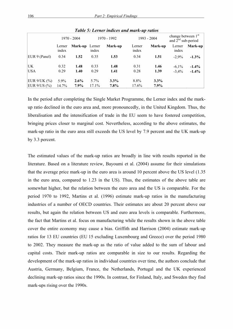
106 Part 2: Empirical Findings
Table 5: Lerner indices and mark-up ratios
1970 - 2004 1970 - 1992 1993 - 2004 change between 1st and 2nd sub-period
Lerner index
Mark-up Lerner index
Mark-up Lerner index
Mark-up Lerner index
Mark-up
EUR 9 (Panel) 0.34 1.52 0.35 1.53 0.34 1.51 -2,9% -1.3%
UK 0.32 1.48 0.33 1.48 0.31 1.46 -6,1% -1.4% USA 0.29 1.40 0.29 1.41 0.28 1.39 -3,4% -1.4% EUR 9/UK (%) 5.9% 2.6% 5.7% 3.3% 8.8% 3.3% EUR 9/US (%) 14.7% 7.9% 17.1% 7.8% 17.6% 7.9%
In the period after completing the Single Market Programme, the Lerner index and the mark-
up ratio declined in the euro area and, more pronouncedly, in the United Kingdom. Thus, the
liberalisation and the intensification of trade in the EU seem to have fostered competition,
bringing prices closer to marginal cost. Nevertheless, according to the above estimates, the
mark-up ratio in the euro area still exceeds the US level by 7.9 percent and the UK mark-up
by 3.3 percent.
The estimated values of the mark-up ratios are broadly in line with results reported in the
literature. Based on a literature review, Bayoumi et al. (2004) assume for their simulations
that the average price mark-up in the euro area is around 10 percent above the US level (1.35
in the euro area, compared to 1.23 in the US). Thus, the estimates of the above table are
somewhat higher, but the relation between the euro area and the US is comparable. For the
period 1970 to 1992, Martins et al. (1996) estimate mark-up ratios in the manufacturing
industries of a number of OECD countries. Their estimates are about 20 percent above our
results, but again the relation between US and euro area levels is comparable. Furthermore,
the fact that Martins et al. focus on manufacturing while the results shown in the above table
cover the entire economy may cause a bias. Griffith and Harrison (2004) estimate mark-up
ratios for 13 EU countries (EU 15 excluding Luxembourg and Greece) over the period 1980
to 2002. They measure the mark-up as the ratio of value added to the sum of labour and
capital costs. Their mark-up ratios are comparable in size to our results. Regarding the
development of the mark-up ratios in individual countries over time, the authors conclude that
Austria, Germany, Belgium, France, the Netherlands, Portugal and the UK experienced
declining mark-up ratios since the 1990s. In contrast, for Finland, Italy, and Sweden they find
mark-ups rising over the 1990s.

Spillover from economic reform 107
Summing up, while the levels of our mark-up ratios seem to be at the upper bound of values
found in the literature, the relation between the euro area and the US is broadly in line with
findings in existing studies.
As a complement to the summary results of table 4, the following figures show the trajectories
of the mark-up ratios in the nine euro area countries in the panel over the period 1971 to 2004.
For comparison, the evolution of the mark-ups in the UK and the US is also displayed. For
this analysis, time series of the mark-up ratios for the countries under consideration are
needed. The mark-up ratios shown in the table above have been estimated for two sub-
periods. For the subsequent analyses, rolling regressions have been performed for each
country in the panel. The estimations were based on equation (6.6) above. The first regression
was run for the ten-year period 1961 to 1970, and the value of the mark-up was assigned to
the final year of this period. In each of the subsequent regression runs, the starting and the
terminal point were moved forward by one year, and the result was again assigned to the final
year of the respective period. This procedure resulted in time series for the mark-up ratios
from 1970 to 2004.38
In order to remove outliers in the time series and to derive smoother time paths for the
following figures, moving four year averages have been calculated. The first values shown in
the graphs cover the period 1971 to 1974.
38 Due to data availability, the mark-up time series for Finland and Ireland start in 1977.

108 Part 2: Empirical Findings
Figure 16: Evolution of mark-up in selected euro area countries
AT - Austria, BE - Belgium, FI - Finland, NL - Netherlands, IE – Ireland
Figure 17: Evolution of mark-up in selected euro area countries, cont’d
DE - Germany, ES - Spain, FR - France, IT - Italy
1.1
1.3
1.5
1.7
1.919
74
1976
1978
1980
1982
1984
1986
1988
1990
1992
1994
1996
1998
2000
2002
2004
AT BE FI NL IE
1.2
1.4
1.6
1.8
2.0
2.2
1974
1976
1978
1980
1982
1984
1986
1988
1990
1992
1994
1996
1998
2000
2002
2004
DE ES FR IT

Spillover from economic reform 109
Figure 18: Evolution of mark-up in the euro area, the US and the UK
EUR9 - panel of the nine euro area countries of the previous figures, US - United States,
UK - United Kingdom
In Austria, Ireland, and France, the mark-up ratios exhibit clearly negative trends over the
entire period. In Belgium, Italy, and, albeit to a much lesser extent, in Spain, the mark-up first
declined, then rose remarkably around the middle of the period, before decreasing again
towards the end of the period. In the Netherlands, the mark-up has remained virtually constant
and low as compared to the other euro area countries. For Finland, we find a significant
decrease of the mark-up until the beginning of the 1990s. Afterwards, it rose again somewhat,
but remained at the lower end of the spectrum. In Germany, the mark-up ratio increased
somewhat in the most recent period, after having been on a decreasing trend until the middle
of the 1990s. The German pattern might be related to the restructuring of Eastern German
industry after unification. Despite the increase in the most recent years, the mark-up in
Germany has remained relatively low. As can be clearly seen, the mark-up in the US has been
below European levels since the beginning of the 1980s, and the downward trend has been
more distinct as compared to the euro area. The UK exhibits increasing mark-up ratios until
the beginning of the 1990s and a downward trend afterwards. In the continental European
countries, the decrease in the mark-up ratios began in the second half of the 1980s.
1.3
1.4
1.5
1.6
1.719
74
1976
1978
1980
1982
1984
1986
1988
1990
1992
1994
1996
1998
2000
2002
2004
EUR9 US UK

110 Part 2: Empirical Findings
The following sections analyse the influence of the mark-up on the macroeconomic
performance as well as the link between product and factor market institutions and the mark-
up ratios.
6.3 The link between the mark-up and macroeconomic performance
In this section, the influence of the mark-up ratio on important macroeconomic indicators is
analysed by means of panel estimations39. Macroeconomic indicators comprise total factor
productivity growth, labour productivity growth, employment and unemployment. The
subsequent estimations have been performed for the panel of nine euro area countries. The
starting point is 1976 (1975 in some cases), i.e. after the recession caused by the first oil price
shock. The termination points of the estimations depend on data availability. While
macroeconomic variables are available until 2004, the time series of product and factor
market indicators end in 2002, in some cases in 1999.
Previous studies conclude that structural reforms such as the Single Market Programme could
increase the long-run level of total factor productivity in the EU by 0.5 to 1 percent (European
Commission, 2004). Simulating a 10 percentage point cut in the mark-up brought about by
product market reforms, the IMF (2003) concludes that in the long-run, GDP could increase
by 4.3 percent. Also based on model simulations, Bayoumi et al. (2004) estimate that
reducing the mark-up in the euro area to the US level would raise GDP in the long run by 8.6
percent.
Total factor productivity growth
The analysis of the link between the mark-up of prices over marginal cost and the
macroeconomic performance begins with total factor productivity (TFP) growth. TFP can be
viewed as an indicator for technical progress and is an important determinant of economic
growth. According to IMF estimates, GDP per capita in the euro area grew in the period 1995
to 2003 by 1.7 percent per annum, compared to 2.4 percent in the United States. This gap
between the two areas can to a large extent be traced back to a divergent development of total
factor productivity. In the period under consideration, TFP growth reached 0.8 percent per
annum on average in the euro area, far behind the 1.4 percent per annum recorded in the
United States (Estevao, 2004). Not only does the TFP growth rate in the euro area lag behind
the US, total factor productivity growth in most of the euro area countries has also declined
39 The estimations have been performed with the software package EViews 4.1.

Spillover from economic reform 111
over time. According to our calculations, TFP growth in the aggregate of the nine euro area
countries under consideration decreased from nearly 5 percent per annum in the 1970s to less
than two percent per year in the period 1995 to 2004. In the four largest euro area economies
(Germany, France, Italy, and Spain), TFP growth fell from more than 5 percent per annum in
the 1970s to only 1¼ percent annually in the most recent decade.
One important source of the rather unsatisfactory growth performance of the euro area, in
particular compared to the United States may be found in the less competitive environment,
visible in higher mark-up ratios. TFP growth can be interpreted as an indicator of dynamic
efficiency. The level of competition, reflected in the mark-up ratio, influences dynamic
efficiency through incentives to engage in innovation activities (Griffith and Harrison, 2004).
However, from a theoretical point of view it is not unambiguously clear that lower economic
rents positively affect dynamic efficiency. This is because a higher degree of competition
reduces the gains from innovation. Early publications on endogenous growth and industrial
organisation suggested that increased product market competition negatively influences
innovation and thus TFP growth as more competition diminishes possible rents to be accrued
by innovators. These results rest upon the assumption that only outsiders engage in innovation
activities. Thus, in these models, rents prior to innovation are zero, and the total extra profit to
be earned by innovation is equal to post-innovation rents. Therefore, incentives to innovate
are positively correlated with rents. Under these assumptions, product market reforms that
reduce rents decrease innovation and thus dynamic efficiency.
More recent endogenous growth models extend the basic Schumpeterian model by allowing
not only outsiders but also incumbent firms to innovate. As insiders also innovate, pre-
innovation rents are not zero, but positive. In this case, fostering competition may reduce pre-
innovation rents by more than post-innovation rents. Thus, mark-up reducing reforms may
have a positive influence on dynamic efficiency, i.e. raise TFP growth.
As these theoretical considerations have shown, the link between the degree of competition
and dynamic efficiency may either be positive or negative. Thus, in this section the
relationship between the mark-up ratios in the EUR 9 and TFP growth are investigated
empirically.

112 Part 2: Empirical Findings
The calculation of TFP growth was based on the growth accounting framework, assuming a
Cobb-Douglas production function with constant returns to scale. TFP growth can be
identified as that part of real GDP growth which is not explained by increases in the
production factors., Labour, capital, and technical progress, i.e. TFP, have been taken into
consideration as input factors. Capital input was approximated by the capital stock in the
business sector, deflated by the GDP deflator. As already mentioned above, consistent OECD
data on capital stocks are only available for the business sector, but not for the entire
economy. For reasons of consistency, employment was approximated by the number of
employees in the business sector only.
Total income is given by the sum of “compensation of employees” and “income from
property and other”, the latter approximating capital income. Thus, labour input was derived
by multiplying the number of employees by the share of compensation of employees in total
income, while capital input is given by the real capital stock, multiplied by the share of
income from property and other in total income. The residual GDP growth not accounted for
by labour and capital input, i.e. the Solow residual, can be identified as TFP growth.
The estimation was performed with fixed country effects and with the lagged endogenous
variable.40 Using random effects resulted in an insignificant coefficient of the mark-up.
Random effects would only work without the lagged endogenous variable, but in this case
there would be problems with serial correlations of the residuals. The results in the box below
show that the influence of the mark-up ratio of prices over marginal cost on TFP growth is
significantly negative. According to the estimates presented, and taking into account the
average values of the mark-ups in the countries under consideration, a reduction of the mark-
up in the euro area by around 10 percent (which, according to the estimates presented in
section 6.2, is about the gap to the US level) would raise average TFP growth in the euro area
by 0.57 percentage points (pp). Looking at the Member States, the effect ranges from 0.5 pp
in Finland and the Netherlands to 0.75 pp in Italy.
40 As already mentioned in chapter 5, including a lagged endogenous variable in a fixed-effects model may result in biased and inconsistent estimates However this bias is small if the cross-section dimension is small in relation to the time dimension of the panel. This is clearly the case here

Spillover from economic reform 113
Dependent variable: TFP growth rate (GTFP) Variable Coefficient t-statistic (absolute value) GTFP-1 0.240** 4.033 MARKUP -3.448** 3.169 Fixed Effects Austria 6.797 Belgium 6.464 Germany 6.230 Spain 6.925 Finland 7.583 France 6.966 Ireland 8.953 Italy 9.006 Netherlands 6.306 Sample 1976 - 2004 Observations 257 R² 0.234 F-statistic 8.816 Durbin-Watson 1.897 ** denotes significance at the 1 percent level.
Employment
In addition to TFP, employment can be expected to be influenced by the degree of
competition as captured by the mark-up ratio. Blanchard and Giavazzi (2001) consider a
model with a product market which is characterised by monopolistic competition. The
elasticity of demand is assumed to depend negatively on the degree of product market
regulation. This negative relationship can be explained by the notion that demand elasticity is
an increasing function of the number of firms. The latter in turn depends negatively on the
cost of entry. Thus, removing barriers to entry increases the number of firms, which raises the
elasticity of demand and thus lowers the level of rents in the economy. In this context, firms
choose labour to maximise the present discounted value of future cash flow. Changing
employment causes adjustment costs. The authors assume that these adjustment costs can be
affected by product market regulation. The model generates predictions about the relationship
between product market regulation, the mark-up (or the level of rents) and the level of
employment. Deregulation, by reducing the mark-up, leads to a higher demand for labour.
Another reason for a negative relationship between the mark-up and employment is that
economies of scale should disappear as a result of emerging new technologies (Coppens and
Vivet, 2004). If sunk costs are low and entry and exit barriers are reduced, the number of
firms increases, entailing a positive impact on job creation. Employment is also supported by

114 Part 2: Empirical Findings
the fact that lower profit margins are accompanied by lower real wage claims and thus by
reduced structural unemployment. More competition in product markets tends to lead to lower
wage mark-ups. Thus, the price mark-up and the wage mark-up are generally positively
related, and reforms diminishing the former also lead to declines of the latter.
For the panel of nine euro area countries, the following box shows that employment is indeed
negatively influenced by the mark-up.41 The low Durbin Watson statistic in combination with
the high coefficient of determination points to some problems with the regression. However,
using the growth rate instead of the level of employment or including the lagged dependent
variable resulted in an insignificant coefficient of the mark-up. The regression has been
performed with fixed country effects. A random effects estimation leads to almost exactly the
same results. Based on the Hausman test, the specification with fixed effects was preferred.
Bringing the mark-up in the countries of the euro area to US levels would raise employment
in the euro area by about 2.7 percent. In the first quarter 2005, about 137.2 million people in
the euro area were in paid employment. The simulated cut of the mark-up by 10 percent could
therefore raise employment to about 141 million.
Dependent variable: logarithm of employment ln (emp) Variable Coefficient t-statistic (absolute value) ln (MARKUP) -0.251** 2.853 Fixed Effects Austria 15.260 Belgium 15.272 Germany 17.377 Spain 16.492 Finland 14.722 France 17.023 Ireland 14.199 Italy 17.000 Netherlands 15.794 Sample 1976 - 2004 Observations 259 R² 0.991 F-statistic 3019.5 Durbin-Watson 0.067 ** denotes significance at the 1 percent level.
41 Here, the logarithm has been used in order to take the different orders of magnitude of the variables into account.

Spillover from economic reform 115
Unemployment rate
An increase in employment brought about by enhanced competition and thus a decrease in the
mark-up of prices over cost would also reduce unemployment. But the decline of
unemployment is not symmetric to the increase in employment. When employment rises,
more people engage in actively seeking employment as they see improving opportunities on
the labour market. Therefore, the decline in unemployment is typically less pronounced than
the increase in employment. Thus, a separate panel estimation has been performed for the
relationship between the unemployment rate and the mark-up. Again, the model includes
fixed country effects. A random effects estimation produced almost the same results; the
Hausman test suggests that the fixed effects model is superior. The low Durbin Watson
statistic points to problems with serial correlation. However, this phenomenon cannot be
alleviated by including the lagged unemployment rate. Furthermore, in the latter case the
mark-up becomes insignificant.
Taking the estimation results shown below into account, cutting the mark-up in the euro area
by 10 percent would result in a decline in the average unemployment rate by about 0.5
percentage points. Among the member countries, the effect ranges from 0.4 percentage points
in Finland to 0.65 percentage points in Italy.
In the first eight months of 2005, the average euro area unemployment rate amounted to 8.8
percent. According to the estimation results, a cut of the mark-up by 10 percent could thus
reduce the unemployment rate to about 8.3 percent.

116 Part 2: Empirical Findings
Dependent variable: unemployment rate (UR) Variable Coefficient t-statistic (absolute value) MARKUP 3.306* 2.214 Fixed Effects Austria -1.393 Belgium 3.607 Germany 1.755 Spain 8.154 Finland 3.817 France 4.020 Ireland 5.491 Italy 2.767 Netherlands 1.444 Sample 1975 - 2004 Observations 266 R² 0.493 F-statistic 29.615 Durbin-Watson 0.154 *denotes significance at the 5 percent level.
Labour productivity growth
Besides total factor productivity and employment, labour productivity is an important
macroeconomic indicator. If real wages increase in line with labour productivity growth, unit
labour costs remain constant. Thus, rising labour productivity growth widens the scope for
wage increases. According to IMF estimates, labour productivity growth in the euro area lags
considerably behind the US (Estevao, 2004). Between 1995 and 2003, output per employee
expanded by 1.2 percent per annum in the euro area and by 2.1 percent annually in the US. In
addition, while in the US labour productivity growth accelerated in the second half of the
1990s, in the euro area it declined considerably.
Lack of competition in the goods and labour markets, leading to higher mark-ups of prices
over cost may be a reason for the less favourable productivity performance in the euro area as
compared to the United States. Griffith and Harrison (2004) find a positive relationship
between the mark-up and the level of labour productivity, but a negative influence on the
growth rate .The authors explain the positive influence of economic rents on the productivity
level by recourse to the job creation effect of lower mark-ups. If new workers entering the
workforce are less productive than incumbents, then the overall productivity level declines.
The same effect can be observed if new jobs are created in less productive sectors. This notion
seems realistic because the more productive workers and firms have already been in place at

Spillover from economic reform 117
higher mark-up levels. However, the link between economic rents and the growth rate of
labour productivity may still be negative. If the productivity of newly created jobs is lower
than that of existing jobs, then a rise in employment as a result of lower mark-ups will be
associated with a reduction in labour productivity growth, but only while employment is
growing. Once employment has reached its new - higher - level, the growth rate of labour
productivity may rise again, even though the level of labour productivity may remain lower
for some time.
The following section investigates the influence of the mark-up on the growth rate of labour
productivity. The latter is defined as real GDP per employee. For the estimation, the
cyclicality of labour productivity growth has been removed by taking the growth rate of trend
rather than actual labour productivity. The trend has been determined by applying the
Hodrick-Prescott filter. The following box shows the estimation results. Based on the
Hausman test, the estimation was performed with fixed country effects. As in the employment
equation, the low Durbin Watson statistic cannot be improved upon by including the lagged
dependent variable. In addition, the latter results in an insignificant mark-up ratio.
Dependent variable: trend labour productivity growth rate (GTRENDPROD) Variable Coefficient t-statistic (absolute value) MARKUP -1.015** 3.041 Fixed Effects Austria 3.515 Belgium 3.307 Germany 2.479 Spain 3.211 Finland 3.698 France 3.116 Ireland 5.025 Italy 3.685 Netherlands 2.466 Sample 1976 - 2004 Observations 259 R² 0.547 F-statistic 35.556 Durbin-Watson 0.039 ** denotes significance at the 1 percent level.
As can be seen, the negative influence of the mark-up on the development of trend labour
productivity is highly significant. According to the above results of the panel estimation, a
reduction of the mark-up in the euro area by 10 percent would raise the growth rate of trend

118 Part 2: Empirical Findings
labour productivity by 0.15 percentage points (pp). The effect would lie in the range of 0.13
pp in the Netherlands to 0.2 pp in Italy.
6.4 The influence of regulation on the mark-up
After having analysed the influence of the mark-up on the macroeconomic performance, this
section looks at the link between institutions and the mark-up ratios. The institutional
framework is an important determinant of the degree of competition. The latter in turn
determines the scope for setting prices significantly above marginal cost and thus exploiting
economic rents. According to previous studies, institutional reforms could lead to mark-up
reductions in the European Union of between 0.5 and 0.9 percentage points (European
Commission, 2004).
Labour market institutions used in the subsequent regression comprise the unemployment
benefit replacement rate (BRR), the benefit duration index (BD), and an index measuring the
degree of wage bargaining coordination (CO). The benefit replacement rate is defined as the
unemployment benefit in the first year as a percentage of average earnings before tax. The
benefit duration index is a weighted average of the ratio between the unemployment benefit in
the second and first years and the ratio between the unemployment benefit in the fourth and
first years. The wage bargaining coordination index lies in the range of 1 to 3, increasing in
the degree of coordination in the wage bargaining process on the employers’ as well as on the
unions’ side. Details on the definition and construction of these indicators can be found in
Nickell and Nunziata (2001) and in Nickell (2003).
A highly regulated labour market allows employers’ and employees’ associations to share
economic rents. Labour market regulations protecting workers or providing generous benefits
to unemployed persons tend to increase the reservation wage, thus leading to higher wage
claims. As a result, wages tend to be higher and employment would be lower than under more
intensive competition; the deviation of prices from marginal cost widens (Nunziata, 2001). In
a more competitive environment, the scope for such behaviour would be smaller. Thus, both
the benefit duration index and the benefit replacement rate should positively influence the
mark-up. In contrast, a higher degree of wage bargaining coordination would allow account to
be taken of economy-wide developments in the wage negotiations. Thus, a higher degree of
coordination would reduce the wage pressure and thus the mark-up (see, e.g., Nunuziata,
2001). On the other hand, not only a high but also a low level of wage bargaining

Spillover from economic reform 119
coordination may lead to wage restraint as in this case firm-specific developments can be
taken into account. Thus, both a highly centralised and a largely decentralised wage
bargaining process seem to dominate the intermediate case, where the advantages of both
systems cannot be fully exploited and wages tend to be too high (Calmfors and Driffill, 1988).
In addition to labour market institutions, an index measuring the openness to international
trade (TRADE) has been included in the estimation. This index was taken from the Fraser
Institute database (Gwartney and Lawson, 2004). Including this indicator is based on the
notion that a high degree of actual or potential international competition reduces the scope for
companies to set prices above marginal cost, and therefore a negative influence on the mark-
up is to be expected.
Other labour market indicators that are published by Nickell and Nunziata (2001), such as
union density, an indicator measuring the degree of employment protection, or the tax wedge
on labour income, proved to be insignificant or had an economically implausible sign.
The following box shows the estimation results. The regression was run with fixed country
effects. If random effects were used, the benefit duration and the trade variables become
insignificant. Including the lagged mark-up also resulted in insignificant coefficients. As was
to be expected, both higher benefit replacement rates and longer unemployment benefit
durations lead to larger mark-up ratios. On the other hand, more openness to international
trade and thus international competition reduces the mark-up. The respective coefficient is
almost significant at the 1 percent level. In addition, a higher degree of coordination in the
wage bargaining process negatively influences the mark-up. The hump shaped hypothesis, i.e.
the notion that both lower and higher degrees of wage bargaining coordination are superior to
an intermediate solution could not be confirmed.

120 Part 2: Empirical Findings
Dependent variable: mark-up Variable Coefficient t-statistic (absolute value) BRR 0.486** 5.085 BD 0.376** 3.209 CO -0.084** 2.965 TRADE -0.047* 2.397 Fixed Effects Austria 1.521 Belgium 1.562 Germany 1.605 Spain 1.719 Finland 1.435 France 1.486 Ireland 1.855 Italy 2.277 Netherlands 1.360 Sample 1976 - 1999 Observations 214 R² 0.688 F-statistic 40.110 Durbin-Watson 0.416 *, ** denotes significance at the 5, 1 percent level.
In 1999, the last year for which data on labour market institutions is available in Nickell
(2003), the benefit replacement rate BRR in the nine euro area countries considered in the
estimation amounted to 0.52 on average. This value compares to 0.29 in the United States and
just 0.17 in the United Kingdom. Thus, not only compared to the US, but also to the UK,
unemployment benefits are more generous in the euro area. Simulations show that a reduction
of the benefit replacement rate in the euro area by 25 percent would result in a decline of the
mark-up ratio by 4.3 percent on average. In 1999, the average value of the benefit duration
index BD took the value 0.56 in the euro area, compared to 0.22 in the US. A 25 percent
reduction in the benefit duration variable would lead to a decline of the average euro area
mark-up by 3.7 percent. Both the wage bargaining coordination and the openness to
international trade are already comparatively high in the euro area.
As an alternative to using detailed variables measuring the labour market regulation, an
overall index could be applied. Such a summary index is contained in the database of the
Fraser Institute. This indicator (LREG) takes values between 1 and 10, rising with the degree
of economic freedom, i.e. the index decreases with increasing labour market regulation. It
consists of the following five sub-indices (Gwartney and Lawson, 2004):

Spillover from economic reform 121
i. Impact of minimum wage: the minimum wage, set by law, has little impact on wages
because it is too low or not obeyed.
ii. Hiring and firing practices: hiring and firing practices of companies are determined by
private contract.
iii. Share of labour force whose wages are set by centralised collective bargaining.
iv. Unemployment benefits: the unemployment benefits system preserves the incentive to
work.
v. Use of conscripts to obtain military personnel.
In the nine euro area countries under consideration, the index had an average value of 4.3 in
2002, compared to 7.3 in the US. Thus, labour markets in the euro area are more regulated
than in the United States. In the UK, the indicator amounts to 6.7. Thus, the UK labour market
is more flexible than the labour markets in the euro area countries, but it is significantly more
regulated than its US counterpart. Although over time the indicator has risen in the euro area
countries, in the UK and in the US it increased to a larger extent. In the latter two countries,
the share of the labour force whose wages are set by centralised wage bargaining has
declined, and the unemployment benefit system has become less generous. As a result of the
former development, economic conditions of the individual companies can better be taken
into account, while the latter effect reduces the reservation wage. Both effects reduce the
scope for workers to exploit economic rents, thus decrease wage pressure.
Using this summary labour market regulation indicator instead of the more detailed variables
taken in the previous regression resulted in significant coefficients with the economically
correct sign only if country-specific time trends were included.42 Other variables on product
and factor market regulation that are also published by the Fraser Institute, such as the
openness to international trade, ease of starting a new business, overall business regulation,
size of government or the overall freedom of the world index are either available for too short
a time span or resulted in coefficients that were insignificant or had an economically
implausible sign.
The following box shows the estimation results. Again, the low Durbin Watson statistic points
to problems with serial correlation. However, including the lagged dependent variable cannot
alleviate this problem. If the lagged mark-up but not the time trends are included, the labour
42 All other estimations discussed in this chapter have been performed without country-specific time trends.

122 Part 2: Empirical Findings
market regulation variable becomes insignificant. Overall, the estimation results show that the
above specification with more detailed labour market regulation indicators is superior.
Dependent variable: mark-up Variable Coefficient t-statistic (absolute value) LREG -0.069** 3.587 Country-specific time trends Austria -0.007** 3.624 Belgium 0.017** 7.079 Germany -0.006** 3.097 Spain -0.005* 2.154 Finland -0.006** 2.656 France -0.001 0.420 Ireland -0.014** 5.841 Italy 0.022** 10.390 Netherlands 0.008** 2993 Fixed Effects Austria 1.950 Belgium 1.275 Germany 1.842 Spain 1.727 Finland 1.802 France 1.681 Ireland 2.494 Italy 1.511 Netherlands 1.306 Sample 1975 - 2002 Observations 248 R² 0.809 F-statistic 59.167 Durbin-Watson 0.583 *, ** denotes significance at the 5, 1 percent level.
Taking, nevertheless, these estimation results into account, decreasing the labour market
regulation in the nine euro area countries considered in the panel estimation to the US level
would result in a decline in the average euro area mark-up by about 14 percent or 0.2
percentage points. Among the Member States the reduction ranges from 7 percent (0.11
percentage points) in Ireland to about 24 percent (0.33 percentage points) in Germany.

Spillover from economic reform 123
6.5 Summary of effects of structural reforms
This section summarises the results of the preceding panel analyses. Here, the effects of
structural reforms on the macroeconomic performance are shown for the aggregate euro area.
In the next chapter, the issue of international spillover between the euro area countries will be
addressed by means of simulations of a multi-country model. The following table shows the
effects of labour market deregulation on the mark-up.
Table 6: Effects of deregulation on the mark-up
Reduction of benefit replacement rate by 25 percent
Reduction of benefit duration index by 25 percent
Mark-up 4.3 percent decline 3.7 percent decline According to these results, making the unemployment benefit system in the euro area less
generous could be expected to result in a decline of the average euro area mark-up ratio by
around 4 percent.
The following table summarises the influence of the mark-up on the macroeconomic
performance. In particular, the effects of a 10 percent cut in the average euro area mark-up on
TFP growth, labour productivity growth, employment, and unemployment are shown.
Table 7: Macroeconomic effects of a 10 percent cut in the euro area mark-up
Indicator Effect TFP growth rate 0.57 percentage points increase Labour productivity growth rate 0.15 percentage points increase Employment 2.7 percent increase Unemployment rate 0.5 percentage points decline
As the table shows, a 10 percent reduction of the euro area mark-up, bringing prices closer to
marginal cost, would boost total factor productivity growth by 0.57 percentage points. Labour
productivity growth would increase by 0.15 percentage points. In addition, a positive
employment effect can be expected: employment would rise by 2.7 percent, and the
unemployment rate would be half a percentage point lower.
The issue of the way in which the macroeconomic performance and fiscal policies in the other
euro area countries would be affected if only one euro area Member State implemented
structural reforms will be one of the subjects to be discussed in the next chapter. There, the
main results of the present chapter will be taken as inputs for simulations with the dynamic,
intertemporal, general-equilibrium multi-region model MSG3. It will be assumed that either
all euro area countries or only one euro area country at a time implements structural reforms
124 Part 2: Empirical Findings
in such a way that the mark-up is reduced by 10 percent and thus TFP growth is raised. These
simulations will be combined with the effects of fiscal discipline, i.e. a combination of
structural reforms and budgetary consolidation.
The model simulations in the next chapter will focus on TFP shocks as results of structural
reforms, as these supply side measures will induce general macroeconomic effects. According
to the estimations in this chapter, cutting the level of the mark-up (a one-time though once-
and-for-all change) has a positive effect on total factor productivity growth. The latter may
mean a one-time effect on the growth of total factor productivity (TFP) or a permanent
increase in the growth rate, which would imply cumulative increases of TFP forever. As we
consider the assumption of an ever-increasing TFP growth rate as far too optimistic (as were
some of the estimates of the European Single Market at the time of the Cecchini Report), it
seems more realistic to assume that TFP will gradually increase to a level higher by 0.57
percent (for the euro area as a whole).

Macroeconomic and welfare effects of structural and budgetary policies 125
7 Macroeconomic and welfare effects of structural and budgetary policies: spillover in the MSG3 model
In this chapter, we aim at analysing and evaluating the macroeconomic effects of structural
policy measures and of policies of budgetary consolidation. For the former, we build upon the
results obtained in chapter 6 regarding the spillover from economic reforms that close the
efficiency gap between the euro area and the US. For the latter, we start from the fact that at
present, several euro area (and other EU) countries have difficulties in fulfilling the deficit
and debt criteria of the Stability and Growth Pact and try to consolidate their budgets. In
chapters 3 and 4, we have provided empirical estimates of the spillover from budgetary
policies that increase the surplus of the public budget, and Appendix 4 gives the
corresponding results for the MSG3 Model. These will be used to run simulations with the
MSG3 Model (see Appendix 3 for more information on this model) that come close to what
we consider as feasible policies. First, we consider structural and budgetary policies
separately, and then we combine both of them. Both isolated (non-coordinated) policy actions
of one country only and coordinated (joint) euro area policies will be investigated. Given the
results of Appendix 4, we will concentrate on isolated policies by Germany and Italy only;
effects for France are between these two, and spillover effects for a small economy (like
Austria) are negligible. In order to arrive at policy recommendations, we will also provide
some tentative welfare calculations comparing different scenarios.
7.1 Effects of structural policies
One of the main results of chapter 6 was an estimate of the effects of deregulation policies in
the euro area on the mark-up in the euro area, which amounted to somewhere between 6 and
14 percent decline. Taking the mean of a 10 percent decline of the mark-up in the euro area,
the effect of this on the total factor productivity growth rate was estimated as an increase by
0.57 percentage points, with some variation between the different countries (Germany 0.57,
France 0.54, Italy 0.75, Austria 0.54 percentage points). We will use these estimates in the
following as inputs into the MSG3 Model. Total factor productivity is an exogenous variable
in this model that can easily be shocked. The other variables possibly affected by the
deregulation reforms (labour productivity, employment, unemployment) are mostly
endogenous variables that will be changed through the channels of the model by changes of
total factor productivity. Estimates of the effects on these variables resulting from the MSG3
Model need not coincide with those from the econometric estimations obtained in chapter 6
because the effects in the MSG3 Model incorporate all kinds of feedbacks from other national

126 Part 2: Empirical Findings
variables and from international spillover effects. Indeed, as we shall see, the effects vary
within the MSG3 simulations depending on the assumptions made about the implementation
of the structural policies under consideration.
Another problem arises from the fact that the econometric estimations of chapter 6 indicate an
effect of cutting the level of the mark-up (a one-time though once-for-all change) on total
factor productivity growth. The latter may mean a one-time effect on the growth of total
factor productivity (TFP) or a permanent increase in the growth rate, which would imply
cumulative increases of TFP forever. We consider the latter interpretation as by far too
optimistic. To be on the safe side, it seems more realistic to assume that TFP will gradually
increase over a period of 5 years to a level higher by 0.57 percent (for the euro area as a
whole; the values for the individual countries are given above) than the baseline and grow
from this higher level with the baseline growth rate later on. These simulations amount to an
increase of TFP by 0.11 percent in the first period, by 0.23 percent in the second, by 0.34
percent in the third, by 0.46 percent in the fourth and by 0.57 percent in the fifth and all
following periods as compared to the baseline solution (numbers for the euro area; numbers
for individual countries differ slightly in accordance with the different long-run values given
above). Alternatives like continued TFP growth by an additional 0.114 percentage points (the
mean additional growth over the first five periods) for each period to follow forever or an
additional growth rate of 0.57 percentage points forever were tried to be simulated, too, but
we arrived at completely unrealistic effects in an unstable model solution, hence these
attempts were discarded. Results from an unstable solution of the model (because the model is
formulated in level terms) are not reliable, and it is highly questionable that one-time (though
permanently upheld) structural reforms will result not only in ever-lasting but even in ever-
increasing gains to the economies affected. Even if this were true, it is not clear whether we
can rely on the results from a local linearisation solution procedure under such a severe
structural change, quite apart from the Lucas critique counter-argument. For these reasons, we
consider results from a TFP shift scenario as described above as much more reliable estimates
of the macroeconomic effects of structural policy reforms. For all simulations in this section,
we assume the policy rule of monetary targeting for euro area monetary policy. The reason for
this is similar to the arguments given in Appendix 4 and will be argued in more detail in
Section 7.4. The following diagrams give again the values of selected endogenous variables
resulting from the simulations. Responses are shown for two countries, namely Germany and
Italy, assuming that only one of these countries implements the deregulation policy leading to

Macroeconomic and welfare effects of structural and budgetary policies 127
the TFP growth according to the estimates, with the other euro area countries going on with
“business as usual” (no economic reforms). Effects in the other countries are purely
international spillover effects. These simulations can be regarded as non-coordinated
structural policies. On the other hand, we also show the effects of a coordinated euro area
economic reform, assuming that all euro area countries implement the policies leading to the
lower mark-up and the higher TFP. The values for other variables as well as results for other
countries and regions of the model are available on request. In the following, we show the
time paths of a few key variables originating from each shock. All numbers are deviations
from the baseline values of the MSG3 Model. In each case, we present (row-wise) the
variables real GDP, current account, budget deficit (general government), public debt (general
government), labour (employment), rate of inflation, short-term and long-term nominal rates
of interest. Countries are denoted by the following symbols: Germany – square, France –
triangle, Italy – asterisk, Austria – circle.

128 Part 2: Empirical Findings
Figure 19: TFP shift, Germany
GDP (real)
-0.1
0
0.1
0.2
0.3
0.4
0.5
0.6
0.7
0.8
0.9
0 5 10 15 20 25 30 35 40 45
Period
Dev
iatio
n [p
erce
nt o
f GD
P]
Current Account (real)
-0.1
-0.05
0
0.05
0.1
0.15
0.2
0.25
0.3
0.35
0.4
0 5 10 15 20 25 30 35 40 45
Period
Dev
iatio
n [p
erce
nt o
f GD
P]
Deficit
-0.4
-0.35
-0.3
-0.25
-0.2
-0.15
-0.1
-0.05
0
0 5 10 15 20 25 30 35 40 45
Period
Dev
iatio
n [p
erce
nt o
f GD
P]
Public Debt
-8
-7
-6
-5
-4
-3
-2
-1
0
0 5 10 15 20 25 30 35 40 45
Period
Dev
iatio
n [p
erce
nt o
f GD
P]
Labour
-0.1
-0.05
0
0.05
0.1
0.15
0.2
0 5 10 15 20 25 30 35 40 45
Period
Dev
iatio
n [p
erce
nt]
Inflation
-0.15
-0.1
-0.05
0
0.05
0.1
0.15
0.2
0 5 10 15 20 25 30 35 40 45
Period
Dev
iatio
n [p
erce
ntag
e po
ints
]
Interest Rate (short, nom.)
-0.08
-0.06
-0.04
-0.02
0
0.02
0.04
0.06
0.08
0.1
0 5 10 15 20 25 30 35 40 45
Period
Dev
iatio
n [p
erce
ntag
e po
ints
]
Interest Rate (long, nom.)
-0.06
-0.05
-0.04
-0.03
-0.02
-0.01
0
0 5 10 15 20 25 30 35 40 45
Period
Dev
iatio
n [p
erce
ntag
e po
ints
]
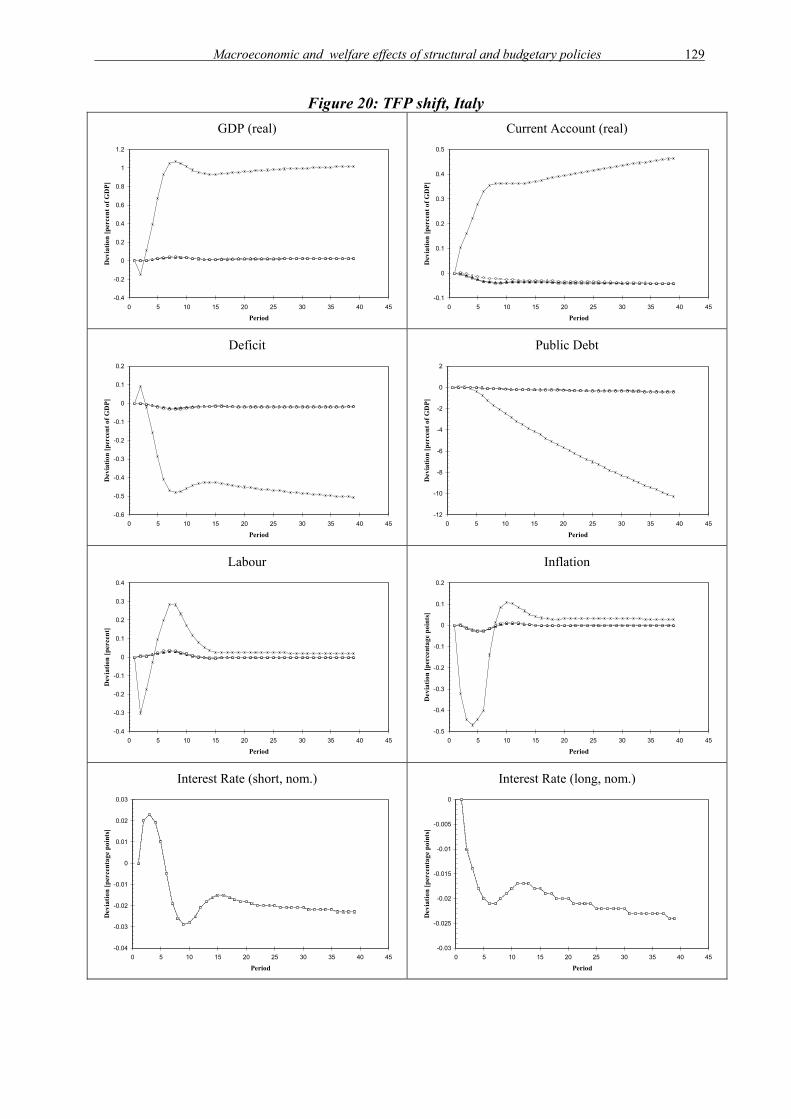
Macroeconomic and welfare effects of structural and budgetary policies 129
Figure 20: TFP shift, Italy GDP (real)
-0.4
-0.2
0
0.2
0.4
0.6
0.8
1
1.2
0 5 10 15 20 25 30 35 40 45
Period
Dev
iatio
n [p
erce
nt o
f GD
P]
Current Account (real)
-0.1
0
0.1
0.2
0.3
0.4
0.5
0 5 10 15 20 25 30 35 40 45
Period
Dev
iatio
n [p
erce
nt o
f GD
P]
Deficit
-0.6
-0.5
-0.4
-0.3
-0.2
-0.1
0
0.1
0.2
0 5 10 15 20 25 30 35 40 45
Period
Dev
iatio
n [p
erce
nt o
f GD
P]
Public Debt
-12
-10
-8
-6
-4
-2
0
2
0 5 10 15 20 25 30 35 40 45
Period
Dev
iatio
n [p
erce
nt o
f GD
P]
Labour
-0.4
-0.3
-0.2
-0.1
0
0.1
0.2
0.3
0.4
0 5 10 15 20 25 30 35 40 45
Period
Dev
iatio
n [p
erce
nt]
Inflation
-0.5
-0.4
-0.3
-0.2
-0.1
0
0.1
0.2
0 5 10 15 20 25 30 35 40 45
Period
Dev
iatio
n [p
erce
ntag
e po
ints
]
Interest Rate (short, nom.)
-0.04
-0.03
-0.02
-0.01
0
0.01
0.02
0.03
0 5 10 15 20 25 30 35 40 45
Period
Dev
iatio
n [p
erce
ntag
e po
ints
]
Interest Rate (long, nom.)
-0.03
-0.025
-0.02
-0.015
-0.01
-0.005
0
0 5 10 15 20 25 30 35 40 45
Period
Dev
iatio
n [p
erce
ntag
e po
ints
]

130 Part 2: Empirical Findings
Figure 21: TFP shift, euro area (coordinated policy) GDP (real)
0
0.2
0.4
0.6
0.8
1
1.2
0 5 10 15 20 25 30 35 40 45
Period
Dev
iatio
n [p
erce
nt o
f GD
P]
Current Account (real)
0
0.05
0.1
0.15
0.2
0.25
0.3
0.35
0.4
0 5 10 15 20 25 30 35 40 45
Period
Dev
iatio
n [p
erce
nt o
f GD
P]
Deficit
-0.6
-0.5
-0.4
-0.3
-0.2
-0.1
0
0 5 10 15 20 25 30 35 40 45
Period
Dev
iatio
n [p
erce
nt o
f GD
P]
Public Debt
-14
-12
-10
-8
-6
-4
-2
0
0 5 10 15 20 25 30 35 40 45
Period
Dev
iatio
n [p
erce
nt o
f GD
P]
Labour
-0.15
-0.1
-0.05
0
0.05
0.1
0.15
0.2
0.25
0.3
0.35
0 5 10 15 20 25 30 35 40 45
Period
Dev
iatio
n [p
erce
nt]
Inflation
-0.5
-0.4
-0.3
-0.2
-0.1
0
0.1
0.2
0.3
0.4
0 5 10 15 20 25 30 35 40 45
Period
Dev
iatio
n [p
erce
ntag
e po
ints
]
Interest Rate (short, nom.)
-0.2
-0.15
-0.1
-0.05
0
0.05
0.1
0.15
0.2
0 5 10 15 20 25 30 35 40 45
Period
Dev
iatio
n [p
erce
ntag
e po
ints
]
Interest Rate (long, nom.)
-0.12
-0.1
-0.08
-0.06
-0.04
-0.02
0
0 5 10 15 20 25 30 35 40 45
Period
Dev
iatio
n [p
erce
ntag
e po
ints
]

Macroeconomic and welfare effects of structural and budgetary policies 131
The results of these simulations can be summarised as follows: Under the TFP shock to a
single country, real GDP of the country directly affected rises over 6 years and stays then at
the higher level forever. Effects are stronger for Italy (GDP above baseline by 1 percent of
baseline GDP) than for Germany (GDP above baseline by 0.7 percent). The current account
improves permanently, the public-sector deficit remains below baseline values, causing public
debt to fall indefinitely (in Italy, it is lower than baseline by 10 percent of baseline GDP after
40 years, in Germany by 8 percent). Employment rises slightly (with a minimal permanent
effect), inflation falls temporarily. Euro area countries not directly affected exhibit only
temporary positive spillover effects to GDP, small permanent negative ones to the current
account and positive ones to the public deficit and public debt. Interest rates rise in the short
run and fall below baseline in the long run. Spillover effects are stronger for Germany than
for Italy due to the size of the economy affected directly. The shock to the entire euro area
brings about positive effects for all euro area countries. Interestingly, also the effects on
Germany and Italy are stronger than in the case where only one of these countries is affected.
Hence, there are positive spillover effects from a coordinated structural policy in the euro
area. For example, GDP remains at higher levels in Germany and Italy than in the case of
isolated structural reforms, and the rates of interest remain below baseline by 0.1 percentage
points, causing public deficits to improve more and public debt to fall by 6 to 12 percent of
baseline GDP after 40 years. These effects are due to positive spillover from the respective
other countries (including the rest of the euro area). For example, if labour market regulations
or price distortions due to imperfect competition are reduced in, say, the Netherlands, this will
support similar measures in Germany by increasing competition also in this country as Dutch
products compete with German ones, inducing further positive supply effects. Hence, there
are truly international feedback effects in addition to direct effects from structural policy
changes.
These results allow a fairly positive evaluation of the effects of structural policies on the euro
area economies. Output will rise to levels permanently above those that would occur without
these reforms, the public deficit will be lower without additional budgetary policy measures,
allowing public debt to decrease over a long time horizon. Spillover effects are not too strong,
but there is some gain from coordinated policies that implement the structural reforms in all
euro area countries as compared to scenarios where these policies are implemented in one or
some countries only. A cautious estimate of a coordinated euro area structural reform scenario
implies a level of GDP that is permanently higher by 1 percent than without these reforms,

132 Part 2: Empirical Findings
virtually without negative effects on other politically relevant variables and with considerable
positive effects on public finances (permanently lower budget deficit, hence cumulatively
lower public debt).

Macroeconomic and welfare effects of structural and budgetary policies 133
7.2 Budgetary consolidation policies
In this section, we analyse some possibilities of policies for budgetary consolidation and their
macroeconomic effects, using the MSG3 Model. It is well known that several euro area
countries have difficulties in meeting the public deficit (3 percent of GDP) and debt (60
percent of GDP) criteria of the Stability and Growth Pact and the requirement to obtain a
balanced budget or even a budgetary surplus over the business cycle and have therefore to
consolidate their budgets. On the other hand, Keynesian macroeconomic theory predicts that
reducing government expenditures or raising taxes in a not fully employed economy will
increase unemployment and reduce economic growth; hence there may be undesirable side-
effects of budgetary consolidation policies. Here we consider two instruments to reduce the
public-sector deficit (and, by this, public-sector debt): decreases of public consumption and
increases of lump-sum taxes (or, equivalently, decreases of lump-sum transfers). The use of
lump-sum taxes is the easiest way to model a tax change within the MSG3 Model as this is a
purely exogenous variable in the MSG3 Model. Simulating such a change shows the
endogenous reactions of other variables that may, in reality, also be influenced by political
actions, such as income or consumption taxes or taxes on particular goods (energy taxes can
be changed in the MSG3 Model). A more elaborate and realistic analysis would simulate
changes of these taxes, too, which would involve re-calibrating the model for each simulation
as for these simulations, parameters (tax rates) instead of exogenous variables would have to
be changed. Lack of time and space prevents such an analysis here; it should be borne in mind
that raising (reducing) lump-sum instead of distortionary taxes underestimates welfare losses
(gains).
As can be seen in Appendix 4, reducing public investment is not to be recommended as a
means of reducing public deficits and debt and is therefore not taken into account here
(although it is often used in actual political processes because it can be relatively easily
changed). In addition to the two instruments mentioned, we also consider a third strategy that
aims at diminishing the size of the public sector by reducing both public consumption and
(lump-sum) taxes. In order to fulfil the aim of consolidating the budget, in this case public
consumption has to be decreased more than taxes, of course.
As for other policies, the time pattern of the policy actions will determine the outcome in
terms of macroeconomic target variables to a large extent. In principle, it is possible to reduce
public expenditures (or raise taxes) by some amount or relative to GDP over a long period in

134 Part 2: Empirical Findings
order to bring public debt down to low values. Such a policy experiment (aiming at
diminishing the size of the public sector) is analysed in Haber et al. (forthcoming 2006) with
unexpectedly strong long-run non-Keynesian effects. However, it may be more realistic to
consider a shorter time horizon for budgetary consolidation. Here we consider a policy change
over 12 years, which may be regarded as corresponding approximately to the length of a full
business cycle or a sequence of three election periods. During the first four years, the budget
deficit is gradually diminished. Then it is kept at lower values for another four years. Finally,
during the last four years, the budget deficit is gradually brought back to the baseline values.
This policy assumption amounts to a temporary budgetary adjustment. As the baseline
solution is a stable adjustment path towards a steady state of the model, it results also in a
permanent fiscal consolidation at a lower level of the debt-to-GDP ratio, which seems to
depict an already ambitious but nevertheless not completely unrealistic program of a
government or an agreement of governments aiming at reversing the growth trend of public
debt that dominated most European countries’ public finances since the first oil price shock in
the 1970s.
In particular, for the first two simulations conducted with the MSG3 Model, we assumed
public consumption to decline, and lump-sum taxes to rise, respectively, by 0.5, 1, 1.5, 2, 2, 2,
2, 2, 2, 1.5, 1 and 0.5 percent of baseline GDP during the 12 years of the budget consolidation
episode. Afterwards, these variables stay at their baseline values forever. For the third
simulation (simultaneous decrease of expenditures and taxes), we assumed reductions of the
two variables in proportion 3:1, i.e., public consumption was decreased by 0.75, 1.5, 2.25, 3,
3, 3, 3, 3, 3, 2.25, 1.5 and 0.75 percent of baseline GDP, with lump-sum taxes declining at the
same time by 0.25, 0.5, 0.75, 1, 1, 1, 1, 1, 1, 0.75, 0.5 and 0.25 percent of baseline GDP
during the 12-years budget consolidation period. The three policy experiments are comparable
as all of them intend to reduce the budget deficit by about 2 percent of GDP over six years,
with a gradual phasing-in and phasing-out. Obviously, a lot of other time profiles are
conceivable, but for the purpose of evaluating the three strategies and their macroeconomic
consequences, we confine ourselves to these scenarios.
As in section 7.1, isolated (non-coordinated) policy actions of one country only and
coordinated euro area policies will be investigated. Again, we concentrate on isolated policies
by Germany and Italy only. Moreover, we assume again the policy rule of monetary targeting
for euro area monetary policy for similar reasons as before. The following diagrams show the

Macroeconomic and welfare effects of structural and budgetary policies 135
values of the same endogenous variables resulting from the three types of simulations as in
section 7.1. Responses are shown for Germany and Italy, assuming that only one of these
countries implements the budgetary consolidation policy, with the other euro area countries
going on with “business as usual” (no change of budgetary policies). Effects in the other
countries are hence again purely international spillover effects. These simulations are
interpreted as budgetary policies without coordination. On the other hand, we also show the
effects of a coordinated euro area budgetary consolidation, assuming that all euro area
countries implement the same budgetary policy strategies. As before, countries are denoted by
the following symbols: Germany – square, France – triangle, Italy – asterisk, Austria – circle.

136 Part 2: Empirical Findings
Figure 22: Budget consolidation, public consumption decrease, Germany GDP (real)
-0.8
-0.6
-0.4
-0.2
0
0.2
0.4
0.6
0.8
1
1.2
0 5 10 15 20 25 30 35 40 45
Period
Dev
iatio
n [p
erce
nt o
f GD
P]
Current Account (real)
-0.6
-0.4
-0.2
0
0.2
0.4
0.6
0.8
1
1.2
1.4
0 5 10 15 20 25 30 35 40 45
Period
Dev
iatio
n [p
erce
nt o
f GD
P]
Deficit
-2
-1.5
-1
-0.5
0
0.5
0 5 10 15 20 25 30 35 40 45
Period
Dev
iatio
n [p
erce
nt o
f GD
P]
Public Debt
-16
-14
-12
-10
-8
-6
-4
-2
0
0 5 10 15 20 25 30 35 40 45
Period
Dev
iatio
n [p
erce
nt o
f GD
P]
Labour
-0.8
-0.6
-0.4
-0.2
0
0.2
0.4
0.6
0.8
1
1.2
0 5 10 15 20 25 30 35 40 45
Period
Dev
iatio
n [p
erce
nt]
Inflation
-1.5
-1
-0.5
0
0.5
1
1.5
0 5 10 15 20 25 30 35 40 45
Period
Dev
iatio
n [p
erce
ntag
e po
ints
]
Interest Rate (short, nom.)
-1.5
-1
-0.5
0
0.5
1
0 5 10 15 20 25 30 35 40 45
Period
Dev
iatio
n [p
erce
ntag
e po
ints
]
Interest Rate (long, nom.)
-0.7
-0.6
-0.5
-0.4
-0.3
-0.2
-0.1
0
0 5 10 15 20 25 30 35 40 45
Period
Dev
iatio
n [p
erce
ntag
e po
ints
]

Macroeconomic and welfare effects of structural and budgetary policies 137
Figure 23: Budget consolidation, public consumption decrease, Italy GDP (real)
-1.5
-1
-0.5
0
0.5
1
1.5
0 5 10 15 20 25 30 35 40 45
Period
Dev
iatio
n [p
erce
nt o
f GD
P]
Current Account (real)
-0.4
-0.2
0
0.2
0.4
0.6
0.8
1
1.2
1.4
1.6
0 5 10 15 20 25 30 35 40 45
Period
Dev
iatio
n [p
erce
nt o
f GD
P]
Deficit
-2.5
-2
-1.5
-1
-0.5
0
0.5
0 5 10 15 20 25 30 35 40 45
Period
Dev
iatio
n [p
erce
nt o
f GD
P]
Public Debt
-16
-14
-12
-10
-8
-6
-4
-2
0
2
0 5 10 15 20 25 30 35 40 45
Period
Dev
iatio
n [p
erce
nt o
f GD
P]
Labour
-1.5
-1
-0.5
0
0.5
1
1.5
0 5 10 15 20 25 30 35 40 45
Period
Dev
iatio
n [p
erce
nt]
Inflation
-1.5
-1
-0.5
0
0.5
1
1.5
0 5 10 15 20 25 30 35 40 45
Period
Dev
iatio
n [p
erce
ntag
e po
ints
]
Interest Rate (short, nom.)
-0.3
-0.25
-0.2
-0.15
-0.1
-0.05
0
0.05
0.1
0.15
0 5 10 15 20 25 30 35 40 45
Period
Dev
iatio
n [p
erce
ntag
e po
ints
]
Interest Rate (long, nom.)
-0.16
-0.14
-0.12
-0.1
-0.08
-0.06
-0.04
-0.02
0
0 5 10 15 20 25 30 35 40 45
Period
Dev
iatio
n [p
erce
ntag
e po
ints
]

138 Part 2: Empirical Findings
Figure 24: Budget consolidation, public consumption decrease, euro area GDP (real)
-1
-0.5
0
0.5
1
1.5
0 5 10 15 20 25 30 35 40 45
Period
Dev
iatio
n [p
erce
nt o
f GD
P]
Current Account (real)
-0.2
0
0.2
0.4
0.6
0.8
1
1.2
0 5 10 15 20 25 30 35 40 45
Period
Dev
iatio
n [p
erce
nt o
f GD
P]
Deficit
-2.5
-2
-1.5
-1
-0.5
0
0 5 10 15 20 25 30 35 40 45
Period
Dev
iatio
n [p
erce
nt o
f GD
P]
Public Debt
-18
-16
-14
-12
-10
-8
-6
-4
-2
0
0 5 10 15 20 25 30 35 40 45
Period
Dev
iatio
n [p
erce
nt o
f GD
P]
Labour
-0.8
-0.6
-0.4
-0.2
0
0.2
0.4
0.6
0.8
1
0 5 10 15 20 25 30 35 40 45
Period
Dev
iatio
n [p
erce
nt]
Inflation
-0.6
-0.4
-0.2
0
0.2
0.4
0.6
0.8
0 5 10 15 20 25 30 35 40 45
Period
Dev
iatio
n [p
erce
ntag
e po
ints
]
Interest Rate (short, nom.)
-2.5
-2
-1.5
-1
-0.5
0
0.5
1
1.5
0 5 10 15 20 25 30 35 40 45
Period
Dev
iatio
n [p
erce
ntag
e po
ints
]
Interest Rate (long, nom.)
-1.4
-1.2
-1
-0.8
-0.6
-0.4
-0.2
0
0 5 10 15 20 25 30 35 40 45
Period
Dev
iatio
n [p
erce
ntag
e po
ints
]

Macroeconomic and welfare effects of structural and budgetary policies 139
Figure 25: Budget consolidation, tax increase, Germany GDP (real)
-0.6
-0.4
-0.2
0
0.2
0.4
0.6
0.8
0 5 10 15 20 25 30 35 40 45
Period
Dev
iatio
n [p
erce
nt o
f GD
P]
Current Account (real)
-0.4
-0.2
0
0.2
0.4
0.6
0.8
1
0 5 10 15 20 25 30 35 40 45
Period
Dev
iatio
n [p
erce
nt o
f GD
P]
Deficit
-2
-1.5
-1
-0.5
0
0.5
0 5 10 15 20 25 30 35 40 45
Period
Dev
iatio
n [p
erce
nt o
f GD
P]
Public Debt
-16
-14
-12
-10
-8
-6
-4
-2
0
0 5 10 15 20 25 30 35 40 45
Period
Dev
iatio
n [p
erce
nt o
f GD
P]
Labour
-0.6
-0.4
-0.2
0
0.2
0.4
0.6
0.8
0 5 10 15 20 25 30 35 40 45
Period
Dev
iatio
n [p
erce
nt]
Inflation
-0.8
-0.6
-0.4
-0.2
0
0.2
0.4
0.6
0.8
0 5 10 15 20 25 30 35 40 45
Period
Dev
iatio
n [p
erce
ntag
e po
ints
]
Interest Rate (short, nom.)
-1
-0.8
-0.6
-0.4
-0.2
0
0.2
0.4
0.6
0 5 10 15 20 25 30 35 40 45
Period
Dev
iatio
n [p
erce
ntag
e po
ints
]
Interest Rate (long, nom.)
-0.5
-0.45
-0.4
-0.35
-0.3
-0.25
-0.2
-0.15
-0.1
-0.05
0
0 5 10 15 20 25 30 35 40 45
Period
Dev
iatio
n [p
erce
ntag
e po
ints
]

140 Part 2: Empirical Findings
Figure 26: Budget consolidation, tax increase, Italy GDP (real)
-1
-0.8
-0.6
-0.4
-0.2
0
0.2
0.4
0.6
0.8
1
0 5 10 15 20 25 30 35 40 45
Period
Dev
iatio
n [p
erce
nt o
f GD
P]
Current Account (real)
-0.2
0
0.2
0.4
0.6
0.8
1
1.2
0 5 10 15 20 25 30 35 40 45
Period
Dev
iatio
n [p
erce
nt o
f GD
P]
Deficit
-2.5
-2
-1.5
-1
-0.5
0
0.5
0 5 10 15 20 25 30 35 40 45
Period
Dev
iatio
n [p
erce
nt o
f GD
P]
Public Debt
-16
-14
-12
-10
-8
-6
-4
-2
0
0 5 10 15 20 25 30 35 40 45
Period
Dev
iatio
n [p
erce
nt o
f GD
P]
Labour
-1
-0.8
-0.6
-0.4
-0.2
0
0.2
0.4
0.6
0.8
0 5 10 15 20 25 30 35 40 45
Period
Dev
iatio
n [p
erce
nt]
Inflation
-1
-0.5
0
0.5
1
1.5
0 5 10 15 20 25 30 35 40 45
Period
Dev
iatio
n [p
erce
ntag
e po
ints
]
Interest Rate (short, nom.)
-0.2
-0.15
-0.1
-0.05
0
0.05
0.1
0 5 10 15 20 25 30 35 40 45
Period
Dev
iatio
n [p
erce
ntag
e po
ints
]
Interest Rate (long, nom.)
-0.12
-0.1
-0.08
-0.06
-0.04
-0.02
0
0 5 10 15 20 25 30 35 40 45
Period
Dev
iatio
n [p
erce
ntag
e po
ints
]

Macroeconomic and welfare effects of structural and budgetary policies 141
Figure 27: Budget consolidation, tax increase, euro area GDP (real)
-0.6
-0.4
-0.2
0
0.2
0.4
0.6
0.8
1
0 5 10 15 20 25 30 35 40 45
Period
Dev
iatio
n [p
erce
nt o
f GD
P]
Current Account (real)
0
0.1
0.2
0.3
0.4
0.5
0.6
0.7
0.8
0.9
0 5 10 15 20 25 30 35 40 45
Period
Dev
iatio
n [p
erce
nt o
f GD
P]
Deficit
-2.5
-2
-1.5
-1
-0.5
0
0 5 10 15 20 25 30 35 40 45
Period
Dev
iatio
n [p
erce
nt o
f GD
P]
Public Debt
-18
-16
-14
-12
-10
-8
-6
-4
-2
0
0 5 10 15 20 25 30 35 40 45
Period
Dev
iatio
n [p
erce
nt o
f GD
P]
Labour
-0.6
-0.4
-0.2
0
0.2
0.4
0.6
0.8
0 5 10 15 20 25 30 35 40 45
Period
Dev
iatio
n [p
erce
nt]
Inflation
-0.5
-0.4
-0.3
-0.2
-0.1
0
0.1
0.2
0.3
0.4
0.5
0 5 10 15 20 25 30 35 40 45
Period
Dev
iatio
n [p
erce
ntag
e po
ints
]
Interest Rate (short, nom.)
-2
-1.5
-1
-0.5
0
0.5
1
0 5 10 15 20 25 30 35 40 45
Period
Dev
iatio
n [p
erce
ntag
e po
ints
]
Interest Rate (long, nom.)
-0.9
-0.8
-0.7
-0.6
-0.5
-0.4
-0.3
-0.2
-0.1
0
0 5 10 15 20 25 30 35 40 45
Period
Dev
iatio
n [p
erce
ntag
e po
ints
]

142 Part 2: Empirical Findings
Figure 28: Budget consolidation, public consumption and tax decrease, Germany GDP (real)
-1
-0.5
0
0.5
1
1.5
0 5 10 15 20 25 30 35 40 45
Period
Dev
iatio
n [p
erce
nt o
f GD
P]
Current Account (real)
-1
-0.5
0
0.5
1
1.5
2
0 5 10 15 20 25 30 35 40 45
Period
Dev
iatio
n [p
erce
nt o
f GD
P]
Deficit
-2
-1.5
-1
-0.5
0
0.5
0 5 10 15 20 25 30 35 40 45
Period
Dev
iatio
n [p
erce
nt o
f GD
P]
Public Debt
-16
-14
-12
-10
-8
-6
-4
-2
0
0 5 10 15 20 25 30 35 40 45
Period
Dev
iatio
n [p
erce
nt o
f GD
P]
Labour
-1
-0.5
0
0.5
1
1.5
0 5 10 15 20 25 30 35 40 45
Period
Dev
iatio
n [p
erce
nt]
Inflation
-1.5
-1
-0.5
0
0.5
1
1.5
0 5 10 15 20 25 30 35 40 45
Period
Dev
iatio
n [p
erce
ntag
e po
ints
]
Interest Rate (short, nom.)
-2
-1.5
-1
-0.5
0
0.5
1
0 5 10 15 20 25 30 35 40 45
Period
Dev
iatio
n [p
erce
ntag
e po
ints
]
Interest Rate (long, nom.)
-0.8
-0.7
-0.6
-0.5
-0.4
-0.3
-0.2
-0.1
0
0 5 10 15 20 25 30 35 40 45
Period
Dev
iatio
n [p
erce
ntag
e po
ints
]

Macroeconomic and welfare effects of structural and budgetary policies 143
Figure 29: Budget consolidation, public consumption and tax decrease, Italy GDP (real)
-1.5
-1
-0.5
0
0.5
1
1.5
0 5 10 15 20 25 30 35 40 45
Period
Dev
iatio
n [p
erce
nt o
f GD
P]
Current Account (real)
-0.4
-0.2
0
0.2
0.4
0.6
0.8
1
1.2
1.4
1.6
1.8
0 5 10 15 20 25 30 35 40 45
Period
Dev
iatio
n [p
erce
nt o
f GD
P]
Deficit
-2.5
-2
-1.5
-1
-0.5
0
0.5
0 5 10 15 20 25 30 35 40 45
Period
Dev
iatio
n [p
erce
nt o
f GD
P]
Public Debt
-16
-14
-12
-10
-8
-6
-4
-2
0
2
0 5 10 15 20 25 30 35 40 45
Period
Dev
iatio
n [p
erce
nt o
f GD
P]
Labour
-1.5
-1
-0.5
0
0.5
1
1.5
0 5 10 15 20 25 30 35 40 45
Period
Dev
iatio
n [p
erce
nt]
Inflation
-2
-1.5
-1
-0.5
0
0.5
1
1.5
2
0 5 10 15 20 25 30 35 40 45
Period
Dev
iatio
n [p
erce
ntag
e po
ints
]
Interest Rate (short, nom.)
-0.3
-0.25
-0.2
-0.15
-0.1
-0.05
0
0.05
0.1
0.15
0 5 10 15 20 25 30 35 40 45
Period
Dev
iatio
n [p
erce
ntag
e po
ints
]
Interest Rate (long, nom.)
-0.18
-0.16
-0.14
-0.12
-0.1
-0.08
-0.06
-0.04
-0.02
0
0 5 10 15 20 25 30 35 40 45
Period
Dev
iatio
n [p
erce
ntag
e po
ints
]
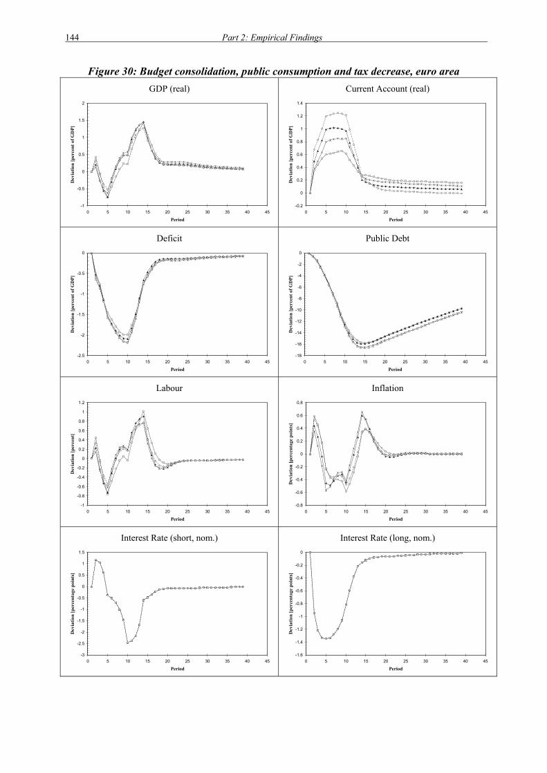
144 Part 2: Empirical Findings
Figure 30: Budget consolidation, public consumption and tax decrease, euro area GDP (real)
-1
-0.5
0
0.5
1
1.5
2
0 5 10 15 20 25 30 35 40 45
Period
Dev
iatio
n [p
erce
nt o
f GD
P]
Current Account (real)
-0.2
0
0.2
0.4
0.6
0.8
1
1.2
1.4
0 5 10 15 20 25 30 35 40 45
Period
Dev
iatio
n [p
erce
nt o
f GD
P]
Deficit
-2.5
-2
-1.5
-1
-0.5
0
0 5 10 15 20 25 30 35 40 45
Period
Dev
iatio
n [p
erce
nt o
f GD
P]
Public Debt
-18
-16
-14
-12
-10
-8
-6
-4
-2
0
0 5 10 15 20 25 30 35 40 45
Period
Dev
iatio
n [p
erce
nt o
f GD
P]
Labour
-1
-0.8
-0.6
-0.4
-0.2
0
0.2
0.4
0.6
0.8
1
1.2
0 5 10 15 20 25 30 35 40 45
Period
Dev
iatio
n [p
erce
nt]
Inflation
-0.8
-0.6
-0.4
-0.2
0
0.2
0.4
0.6
0.8
0 5 10 15 20 25 30 35 40 45
Period
Dev
iatio
n [p
erce
ntag
e po
ints
]
Interest Rate (short, nom.)
-3
-2.5
-2
-1.5
-1
-0.5
0
0.5
1
1.5
0 5 10 15 20 25 30 35 40 45
Period
Dev
iatio
n [p
erce
ntag
e po
ints
]
Interest Rate (long, nom.)
-1.6
-1.4
-1.2
-1
-0.8
-0.6
-0.4
-0.2
0
0 5 10 15 20 25 30 35 40 45
Period
Dev
iatio
n [p
erce
ntag
e po
ints
]

Macroeconomic and welfare effects of structural and budgetary policies 145
The results of these simulations can be briefly summarised as follows: In the country/region
directly affected by the budgetary consolidation policies, all simulations are characterised by a
Keynesian reaction of lower than baseline real GDP and employment in the short run and a
non-Keynesian reaction of higher than baseline real GDP and employment in the medium run.
The former effect is the familiar result of a reduction of (public or private) demand. It occurs
in the MSG3 Model due to its short-run Keynesian features, which were introduced into the
model mainly for reasons of better empirical fit: wages are sticky in the short run, and private
consumption depends not only on wealth but also on current disposable income. The first
feature can be justified by several theoretical arguments (incomplete information of workers,
efficiency wages, insider-outsider theory, etc.), the latter by liquidity constraints of consumers
(in the MSG3 Model, one half of private consumption depends on private wealth, the other
one on current disposable income, which gave the best results when calibrating the model).
Therefore non-Keynesian short-run effects, which have been analysed by some authors,
cannot be observed here.
The medium-run non-Keynesian effect, which in most cases exceeds the short-run Keynesian
effect, is mainly due to the reduction of the public deficit and hence public debt, resulting in
lower rates of interest and higher private wealth; it is also partly due to the increase in
competitiveness as shown by the improved current account. As the budgetary consolidation
policy is modelled as temporary (although over a fairly long time horizon of 12 years), in the
long run the economies return to the baseline path rather quickly after these 12 years. Only
public debt remains permanently well below baseline values (by more than 10 percent of GDP
after 40 years in the case where the budget consolidation policy is most effective; see Figure
30), inducing a (very modest) long-run increase of real GDP over its baseline values. By
contrast, in Haber et al. (2006) we have shown that a permanent reduction of public
consumption and hence the budget deficit can lead to substantial permanent gains in output.
Although the general behaviour of the variables of the countries directly affected by the
policy shock is the same in all simulations considered here, there are some differences in
detail. Comparing the three methods of reducing the budget deficit, we can see that lowering
public consumption and taxes simultaneously gives the strongest effects, followed by
decreasing public consumption only, while lump-sum (net) tax increases result in the weakest
reactions. These differences are not dramatic, however. For example, in the case of budgetary
consolidation for the entire euro area, the maximum reduction of the short-term and the long-
146 Part 2: Empirical Findings
term rate of interest is 2.5 and 1.4 percentage points, respectively, when both public
consumption and taxes are reduced; 2.4 and 1.2 percentage points, respectively, when only
public consumption is reduced; and 1.6 and 0.88 percentage points, respectively, when lump-
sum taxes are increased. Again, it has to be stressed that these simulations are biased against
tax reductions due to the use of lump-sum instead of actual (distortionary) taxes; if the latter
were reduced, consolidating the budget by reducing the size of the public sector through
simultaneous expenditure and (smaller) tax reductions would appear even more favourable.
There are some differences between spillover effects when only one country undergoes the
budgetary consolidation. When Germany is the only country to consolidate, the effects on its
own GDP, employment, current account, public deficit and debt and rate of interest are
weaker than in the case of Italy consolidating its budget. On the other hand, budgetary
consolidation in Germany induces much stronger spillover effects on the other euro area
economies and the common euro area interest rates than budgetary consolidation in Italy,
where the spillover effects are negligible. Spillover effects to GDP, employment and current
account of other euro area countries are anti-symmetric, i.e., they have the opposite signs than
those of the respective own-country effects, reflecting shifts of demand due to both absorption
and relative price effects. When Germany consolidates, the effects on its own inflation rate
are weaker than those on the inflation rates of the other euro area economies, which is due to
the strong first-period spillover effect from German to other euro area countries’ GDP and
employment.
A more interesting distinction can be made between the simulations where only one country
implements the budgetary consolidation policy and those where the entire euro area
consolidates. In the case of a coordinated budgetary consolidation for the entire euro area,
there are gains from coordination: negative short-run Keynesian effects on GDP and
employment are weaker, deficit and debt reduction are stronger and hence medium-run
positive non-Keynesian effects on GDP and employment are also stronger than if one country
only consolidates; this is true also for the respective country (both Germany and Italy in our
simulations). Moreover, inflation oscillates less in the coordinated than in the non-coordinated
scenarios. As for the simulations of structural policies and their effects on TFP, it turns out
that coordinated policy-making brings about a “coordination dividend” for the participating
countries. The reason is the same as for structural policies: If one country pursues an isolated
policy, either of structural reforms or of budgetary consolidation (or both), this will affect this

Macroeconomic and welfare effects of structural and budgetary policies 147
particular country and, via trade and financial flows, to some extent other euro area countries.
But if all euro area countries implement a coordinated policy of the same type, the spillover
effects will reinforce the direct effects. The above-mentioned anti-symmetric effects are
eliminated and even reversed, because now the entire euro area is affected in the same
(desirable) way. Moreover, there may be some effect of increased credibility of such a
coordinated policy, which is not really reflected in the simulations as all policies are assumed
to be credible; hence our results may even underestimate the advantages of a coordinated
policy of the type proposed here.

148 Part 2: Empirical Findings
7.3 Combined structural and budgetary consolidation policies
Next, we investigate macroeconomic results of combining the structural policies analysed in
section 7.1 and budget consolidation policies analysed in section 7.2 with the MSG3 Model.
There are many possibilities of combining these two instruments within the euro area,
depending on which country/region implements which policy. In Appendix 5, we document
the results of all possible combinations of structural policy (the “TFP level shift” version from
section 7.1) with each of the three versions of budgetary consolidation policies (reduction of
public consumption, increase in (net) lump-sum taxes, and simultaneous decrease of public
consumption and of lump-sum taxes) for the countries Germany and Italy and for the euro
area as a whole. We concentrate on Germany and Italy for the same reason why we have
omitted results for France, Austria and REA in the previous sections: The results for France
are in between those for Germany and Italy, those for Austria lack virtually all international
spillover effects (due to the small size of this country’s economy), and those for the REA
block would be completely artificial and not policy-relevant, as this block consists of several
small- and medium-sized economies with fairly different economic and geographical
characteristics (which result in close to euro area average reactions if shocked together,
thereby neglecting the differences between such countries, as, for instance, Ireland, Spain,
Finland and Greece). Again, we assume the policy rule of monetary targeting for euro area
monetary policy. Still, we are left with 27 simulations whose main results are shown in the
following diagrams and those in Appendix 5 for the values of the same endogenous variables
as in sections 7.1 and 7.2. As before, countries are denoted by the following symbols:
Germany – square, France – triangle, Italy – asterisk, Austria – circle. Here, we summarise
only the most relevant results.
In the short-run, policy combinations result in nearly additive combinations of the effects of
the single policies combined. For instance, with respect to GDP and employment, the negative
short-run effect of budgetary consolidation combines with the positive effect of structural
policy to give ambiguous results in the first periods, whereas for public deficit and debt,
inflation and interest rates, the favourable effects of both policies reinforce each others. The
long-run effects are probably more revealing, given the EU political objective of boosting
economic growth during the next decade and beyond, hence we concentrate on them here.
We can distinguish between five main cases, each of which will be illustrated by the results of
one simulation representative of a group containing several others.

Macroeconomic and welfare effects of structural and budgetary policies 149
1. One euro area country only implements both the structural policy and a budgetary
consolidation policy. Take, for example, Germany. The results are shown in Figure 31. Here
budgetary consolidation is achieved by reducing public consumption; if instead taxes are
raised, long-run effects are slightly weaker; if both public consumption and taxes are reduced,
long-run effects are slightly stronger. It can be seen that the combination of structural and
budgetary consolidation policies, even when confined to one single euro area country without
any policy change in other countries, suffices to make higher GDP, higher current account
surplus, lower public budget deficit and lower public debt sustainable in the long run.
Germany obtains real GDP permanently increased above baseline values by 0.8 percent,
current account by 0.5 percentage points of GDP, deficit reduced by 0.5 percent of GDP and
public debt by 15 percent of GDP. If instead of Germany, Italy is the country to conduct these
combined policies, the own-country effects are even higher with 1 percent for GDP, –0.7
percent for the public deficit, and –19 percent for public debt. There are also some permanent
international spillover effects to the other euro area economies: In the case of Germany, the
other countries’ current account deteriorates by about 0.1 percent of GDP, the public deficit is
reduced by 0.1 percent of GDP, public debt is reduced by about 1 percent of GDP, and the
common euro area interest rates are reduced by 0.1 percentage points. These international
spillover effects are much smaller for Italy even though the primary effects of this country’s
policies are stronger than those for Germany (e.g., the rates of interest are only 0.03
percentage points below baseline values in the long run), showing that the size of long-run
international spillover effects depends primarily upon the economic size of a country and its
international trade and financial flows with the other euro area countries and less on the
effectiveness of its policies on its own economy.
2. One euro area country only implements structural policy, another one a budgetary
consolidation policy. Figure 32 shows such a scenario with Italy reducing its public
consumption and Germany conducting the structural policy. In these cases, permanent effects
on GDP are achieved only in the country implementing the structural reform. The output
effects in the country enacting the budgetary consolidation are temporary only. Negative
international spillover effects on the current account are permanent for the countries not
affected by either policy. There is also a weak permanent effect on the rates of interest (about
0.05 percentage points if Germany implements the structural reform, even less if another
country does so instead). This results in a small permanent decrease of the public deficit and

150 Part 2: Empirical Findings
of public debt below baseline for both countries in which policy changes take place and still
smaller ones in the other euro area countries.
3. One euro area country only implements structural policy, the entire euro area implements
a budgetary consolidation policy. Figure 33 shows this scenario under the assumption that it
is Germany that does the structural reform. This combination of policies is sufficient to
generate long-run effects on GDP and the budgetary variables, although these are rather small.
The country that carries out both kinds of policies is clearly better off than the others, both in
the short and in the long run: it enjoys higher GDP, higher current account surplus, lower
public budget deficit and public debt and less volatile inflation. The euro area interest rates
remain below baseline by approximately 0.1 percentage points in the long run. If Italy instead
of Germany is the country implementing structural policies, its own-country effects are
stronger but the international spillover effects in the euro area are considerably smaller than
those from German structural policy reforms.
4. One euro area country only implements a budgetary consolidation policy, the entire euro
area implements structural policy. Figure 34 shows the resulting scenario with Germany
being the budget consolidating country. Now there are permanent favourable effects on GDP
in all countries, especially Germany and Italy. Interestingly, the stronger impulse from Italian
structural reforms makes its long-run GDP rise more above its baseline GDP (in terms of its
own GDP) than that of Germany in spite of the latter’s combined policies. Public deficits
remain below baseline by 0.5 percent of GDP in all countries, public debt is also lower than in
the baseline path (most so, of course, in Germany), and the rates of interest are below by 0.15
percentage points. If Italy instead of Germany is the country consolidating its budget, its
macroeconomic variables fluctuate more than those of Germany in the simulation where
Germany consolidates, the long-run effects on Italy’s GDP are still stronger, and the spillover
effects to other countries are considerably weaker.
5. All euro area countries implement both the structural policy and a budgetary consolidation
policy. This is the ultimate coordinated scenario for the euro area (although it must be noted
that also scenarios assuming common euro area policies in one area only would require a
considerable amount of cooperation to become true in reality). Figure 35 gives the results,
again assuming that budgetary consolidation is done by reducing public consumption. As in
the other four types of scenarios, increasing net lump-sum taxes give slightly weaker,

Macroeconomic and welfare effects of structural and budgetary policies 151
reducing public consumption and taxes slightly stronger effects, but the qualitative pattern of
all macroeconomic variables remains the same, and there are only minor quantitative
differences between the three kinds of budgetary consolidation policies. Figure 35 shows that
in the euro area common policy scenario, real GDP remains above baseline by at least 1
percent for all countries in the long run; for Italy, the corresponding number is even 1.4
percent. Permanent improvements also apply to the current account, the public deficit and
public debt in all euro area countries. The short-run interest rate is below baseline by 0.5
percent, the long-run by 0.2 percent.
The most important lessons from these simulations are the following: in the long run, the
effects of structural policy reforms that increase TFP permanently (even if they raise only its
level) dominate and can bring about a permanent improvement of key macroeconomic target
variables such as output and public finances. In the medium run, budgetary policies are
stronger, but as we have assumed that the budget consolidation will be done over a limited
time period, it exerts nearly no permanent effects (except on public debt) unless supported by
structural reforms. International spillover effects within the euro area are relatively small
(except those from the biggest economy, Germany) and can be advantageous (mostly through
the channel of the common interest rate) or disadvantageous (especially if they affect the
competitiveness of some countries at the expense of other ones within the euro area). As
many other studies on international macroeconomic policy-making have shown, we can
confirm that cooperative policies brought about by policy coordination are superior to non-
cooperative policies, and using two (or more) instruments is superior to relying on one
instrument only. Our results show that the most effective way of achieving permanently
higher output and lower public debt without undesirable side-effects is via a euro area wide
coordinated design of both structural and budgetary consolidation policies. How such
coordination can be achieved is a political question which goes beyond the scope of the
present study.

152 Part 2: Empirical Findings
Figure 31: Public consumption decrease and structural policy in Germany GDP (real)
-0.5
0
0.5
1
1.5
2
0 5 10 15 20 25 30 35 40 45
Period
Dev
iatio
n [p
erce
nt o
f GD
P]
Current Account (real)
-1
-0.5
0
0.5
1
1.5
2
0 5 10 15 20 25 30 35 40 45
Period
Dev
iatio
n [p
erce
nt o
f GD
P]
Deficit
-2.5
-2
-1.5
-1
-0.5
0
0.5
0 5 10 15 20 25 30 35 40 45
Period
Dev
iatio
n [p
erce
nt o
f GD
P]
Public Debt
-20
-18
-16
-14
-12
-10
-8
-6
-4
-2
0
0 5 10 15 20 25 30 35 40 45
Period
Dev
iatio
n [p
erce
nt o
f GD
P]
Labour
-0.8
-0.6
-0.4
-0.2
0
0.2
0.4
0.6
0.8
1
1.2
0 5 10 15 20 25 30 35 40 45
Period
Dev
iatio
n [p
erce
nt]
Inflation
-1.5
-1
-0.5
0
0.5
1
1.5
0 5 10 15 20 25 30 35 40 45
Period
Dev
iatio
n [p
erce
ntag
e po
ints
]
Interest Rate (short, nom.)
-1.5
-1
-0.5
0
0.5
1
0 5 10 15 20 25 30 35 40 45
Period
Dev
iatio
n [p
erce
ntag
e po
ints
]
Interest Rate (long, nom.)
-0.7
-0.6
-0.5
-0.4
-0.3
-0.2
-0.1
0
0 5 10 15 20 25 30 35 40 45
Period
Dev
iatio
n [p
erce
ntag
e po
ints
]

Macroeconomic and welfare effects of structural and budgetary policies 153
Figure 32: Public consumption decrease in Italy, structural policy in Germany GDP (real)
-1.5
-1
-0.5
0
0.5
1
1.5
0 5 10 15 20 25 30 35 40 45
Period
Dev
iatio
n [p
erce
nt o
f GD
P]
Current Account (real)
-0.4
-0.2
0
0.2
0.4
0.6
0.8
1
1.2
1.4
0 5 10 15 20 25 30 35 40 45
Period
Dev
iatio
n [p
erce
nt o
f GD
P]
Deficit
-2.5
-2
-1.5
-1
-0.5
0
0 5 10 15 20 25 30 35 40 45
Period
Dev
iatio
n [p
erce
nt o
f GD
P]
Public Debt
-16
-14
-12
-10
-8
-6
-4
-2
0
0 5 10 15 20 25 30 35 40 45
Period
Dev
iatio
n [p
erce
nt o
f GD
P]
Labour
-1.5
-1
-0.5
0
0.5
1
1.5
0 5 10 15 20 25 30 35 40 45
Period
Dev
iatio
n [p
erce
nt]
Inflation
-1.5
-1
-0.5
0
0.5
1
1.5
0 5 10 15 20 25 30 35 40 45
Period
Dev
iatio
n [p
erce
ntag
e po
ints
]
Interest Rate (short, nom.)
-0.4
-0.3
-0.2
-0.1
0
0.1
0.2
0.3
0 5 10 15 20 25 30 35 40 45
Period
Dev
iatio
n [p
erce
ntag
e po
ints
]
Interest Rate (long, nom.)
-0.25
-0.2
-0.15
-0.1
-0.05
0
0 5 10 15 20 25 30 35 40 45
Period
Dev
iatio
n [p
erce
ntag
e po
ints
]

154 Part 2: Empirical Findings
Figure 33: Public consumption decrease in euro area, structural policy in Germany GDP (real)
-1
-0.5
0
0.5
1
1.5
2
2.5
0 5 10 15 20 25 30 35 40 45
Period
Dev
iatio
n [p
erce
nt o
f GD
P]
Current Account (real)
-0.2
0
0.2
0.4
0.6
0.8
1
1.2
0 5 10 15 20 25 30 35 40 45
Period
Dev
iatio
n [p
erce
nt o
f GD
P]
Deficit
-2.5
-2
-1.5
-1
-0.5
0
0 5 10 15 20 25 30 35 40 45
Period
Dev
iatio
n [p
erce
nt o
f GD
P]
Public Debt
-25
-20
-15
-10
-5
0
0 5 10 15 20 25 30 35 40 45
Period
Dev
iatio
n [p
erce
nt o
f GD
P]
Labour
-0.8
-0.6
-0.4
-0.2
0
0.2
0.4
0.6
0.8
1
0 5 10 15 20 25 30 35 40 45
Period
Dev
iatio
n [p
erce
nt]
Inflation
-0.6
-0.4
-0.2
0
0.2
0.4
0.6
0.8
0 5 10 15 20 25 30 35 40 45
Period
Dev
iatio
n [p
erce
ntag
e po
ints
]
Interest Rate (short, nom.)
-2.5
-2
-1.5
-1
-0.5
0
0.5
1
1.5
0 5 10 15 20 25 30 35 40 45
Period
Dev
iatio
n [p
erce
ntag
e po
ints
]
Interest Rate (long, nom.)
-1.4
-1.2
-1
-0.8
-0.6
-0.4
-0.2
0
0 5 10 15 20 25 30 35 40 45
Period
Dev
iatio
n [p
erce
ntag
e po
ints
]

Macroeconomic and welfare effects of structural and budgetary policies 155
Figure 34: Public consumption decrease in Germany, structural policy in euro area
GDP (real)
-0.2
0
0.2
0.4
0.6
0.8
1
1.2
1.4
1.6
1.8
0 5 10 15 20 25 30 35 40 45
Period
Dev
iatio
n [p
erce
nt o
f GD
P]
Current Account (real)
-0.4
-0.2
0
0.2
0.4
0.6
0.8
1
1.2
1.4
1.6
0 5 10 15 20 25 30 35 40 45
Period
Dev
iatio
n [p
erce
nt o
f GD
P]
Deficit
-2.5
-2
-1.5
-1
-0.5
0
0 5 10 15 20 25 30 35 40 45
Period
Dev
iatio
n [p
erce
nt o
f GD
P]
Public Debt
-20
-18
-16
-14
-12
-10
-8
-6
-4
-2
0
0 5 10 15 20 25 30 35 40 45
Period
Dev
iatio
n [p
erce
nt o
f GD
P]
Labour
-0.6
-0.4
-0.2
0
0.2
0.4
0.6
0.8
1
0 5 10 15 20 25 30 35 40 45
Period
Dev
iatio
n [p
erce
nt]
Inflation
-1.5
-1
-0.5
0
0.5
1
1.5
0 5 10 15 20 25 30 35 40 45
Period
Dev
iatio
n [p
erce
ntag
e po
ints
]
Interest Rate (short, nom.)
-1.5
-1
-0.5
0
0.5
1
0 5 10 15 20 25 30 35 40 45
Period
Dev
iatio
n [p
erce
ntag
e po
ints
]
Interest Rate (long, nom.)
-0.8
-0.7
-0.6
-0.5
-0.4
-0.3
-0.2
-0.1
0
0 5 10 15 20 25 30 35 40 45
Period
Dev
iatio
n [p
erce
ntag
e po
ints
]

156 Part 2: Empirical Findings
Figure 35: Public consumption decrease and structural policy in euro area
GDP (real)
-0.5
0
0.5
1
1.5
2
2.5
0 5 10 15 20 25 30 35 40 45
Period
Dev
iatio
n [p
erce
nt o
f GD
P]
Current Account (real)
0
0.2
0.4
0.6
0.8
1
1.2
1.4
1.6
0 5 10 15 20 25 30 35 40 45
Period
Dev
iatio
n [p
erce
nt o
f GD
P]
Deficit
-3
-2.5
-2
-1.5
-1
-0.5
0
0 5 10 15 20 25 30 35 40 45
Period
Dev
iatio
n [p
erce
nt o
f GD
P]
Public Debt
-25
-20
-15
-10
-5
0
0 5 10 15 20 25 30 35 40 45
Period
Dev
iatio
n [p
erce
nt o
f GD
P]
Labour
-0.6
-0.4
-0.2
0
0.2
0.4
0.6
0.8
1
0 5 10 15 20 25 30 35 40 45
Period
Dev
iatio
n [p
erce
nt]
Inflation
-1
-0.8
-0.6
-0.4
-0.2
0
0.2
0.4
0.6
0.8
0 5 10 15 20 25 30 35 40 45
Period
Dev
iatio
n [p
erce
ntag
e po
ints
]
Interest Rate (short, nom.)
-2.5
-2
-1.5
-1
-0.5
0
0.5
1
1.5
0 5 10 15 20 25 30 35 40 45
Period
Dev
iatio
n [p
erce
ntag
e po
ints
]
Interest Rate (long, nom.)
-1.4
-1.2
-1
-0.8
-0.6
-0.4
-0.2
0
0 5 10 15 20 25 30 35 40 45
Period
Dev
iatio
n [p
erce
ntag
e po
ints
]
Note: Figure 34 and Figure 35 are identical to Figure 93 and Figure 95, respectively, in Appendix 5.

Macroeconomic and welfare effects of structural and budgetary policies 157
7.4 Sensitivity analysis: monetary versus inflation targeting
As can be seen from the diagrams in section 7.1, under the assumption of monetary targeting
(i.e., the ECB sets its money supply for the euro area as in the baseline solution) in no case do
inflation rates of any euro area country exceed 0.4 percentage points above the baseline
solution. In fact, inflation and the price level are lower in all but a few periods for all
countries of the euro area. The reason for this is the fact that the TFP shock is a positive
supply shock that raises output and lowers price level variables. It would be highly
counterproductive if the ECB would, by following a monetary policy rule of inflation
targeting, annihilate these effects by a mostly restrictive policy activism to raise the price
level and the rate of inflation, and we think such a policy of the ECB would be unrealistic
either. Hence, we assume monetary targeting (or an “inactive” monetary policy) here.
Moreover, we know from previous experiments with the MSG Model that under a (positive or
negative) supply shock, “inactive” monetary policy (which is equivalent to monetary targeting
in the framework of the MSG Model) gives results that are superior to those obtained under
an “active” monetary policy (rules like inflation targeting, Taylor rules, nominal income
targeting, exchange rate targeting, etc.); see, e. g., Neck et al. (2004).
The situation is less clear for demand shocks such as those emanating from the budgetary
consolidation, where previous work with the MSG Model did not reveal one particular
monetary policy rule as dominant. Therefore we re-ran several of the experiments of the
previous subsections under the assumptions of monetary policy following a rule of inflation
targeting (keeping euro area inflation at baseline values) and alternatively a rule comparable
to a Taylor rule (a strict Taylor rule cannot be implemented in the MSG Model because
money supply instead of an interest rate is the monetary policy instrument in that model). We
report here only the results of three simulations with inflation targeting as monetary policy
rule for the ECB. Monetary policy of the ECB following a modified Taylor rule (with a non-
negligible weight on euro area real GDP) always resulted in an unstable model solution. The
reason for this is simple: both structural and budgetary consolidation policies as assumed here
result in higher GDP in the medium and long run without negative effects on price level and
inflation rates. In this case, monetary authorities following a mechanical Taylor rule would
implement restrictive policies to reduce real GDP to its baseline values. It is obvious that such
policies were severely misguided and would not be attempted by any reasonable monetary
policy-maker.

158 Part 2: Empirical Findings
Hence we look only at simulations with inflation targeting instead of monetary targeting as
policy rule for the ECB. Inflation targeting is introduced into the model by implementing
dynamic optimisation for the ECB. The ECB is regarded as an active player, adjusting money
supply in order to keep the average euro area inflation rates in each period at the baseline
values (which are close to the 2 percent European inflation target). As inflation is assumed to
be the only objective of the ECB under the monetary policy rule of inflation targeting and
there is one instrument (money supply), the well-known Tinbergen results concerning the
number of instruments and the number of objectives ensure that the inflation target will be
strictly met in all periods. Note that this does not imply zero deviations of the
national/regional inflation rates in all member countries and regions of the euro area, as the
ECB cannot effectively account for differences in regional output and demand. At least for an
asymmetric shock, there will be deviations from the baseline in both directions (positive and
negative), but they will always be smaller than under a monetary targeting regime.
We show the results of structural policy (TFP shock) only and of budgetary consolidation by
reducing public consumption only, both for the case of Germany implementing such a policy,
and the results of combined structural and budgetary consolidation policies for the euro area
in order to illustrate the varieties of isolated versus combined policies and of national versus
coordinated policies. Figure 36 shows the results of structural policies for Germany and
should be compared to Figure 19; Figure 37 shows the result of budgetary consolidation by
reducing public consumption in Germany and should be compared to Figure 22; and Figure
38 shows the results of combined structural and (expenditure-side) budgetary consolidation
policies for the entire euro area and should be compared to Figure 35 as the respective
monetary targeting-counterpart to the inflation targeting rule considered here.

Macroeconomic and welfare effects of structural and budgetary policies 159
Figure 36: TFP shock Germany (inflation target) GDP (real)
-0.1
0
0.1
0.2
0.3
0.4
0.5
0.6
0.7
0.8
0.9
0 5 10 15 20 25 30 35 40 45
Period
Dev
iatio
n [p
erce
nt o
f GD
P]
Current Account (real)
-0.1
-0.05
0
0.05
0.1
0.15
0.2
0.25
0.3
0.35
0.4
0 5 10 15 20 25 30 35 40 45
Period
Dev
iatio
n [p
erce
nt o
f GD
P]
Deficit
-0.4
-0.35
-0.3
-0.25
-0.2
-0.15
-0.1
-0.05
0
0 5 10 15 20 25 30 35 40 45
Period
Dev
iatio
n [p
erce
nt o
f GD
P]
Public Debt
-8
-7
-6
-5
-4
-3
-2
-1
0
0 5 10 15 20 25 30 35 40 45
Period
Dev
iatio
n [p
erce
nt o
f GD
P]
Labour
-0.1
-0.05
0
0.05
0.1
0.15
0.2
0 5 10 15 20 25 30 35 40 45
Period
Dev
iatio
n [p
erce
nt]
Inflation
-0.2
-0.15
-0.1
-0.05
0
0.05
0.1
0.15
0 5 10 15 20 25 30 35 40 45
Period
Dev
iatio
n [p
erce
ntag
e po
ints
]
Interest Rate (short, nom.)
-0.1
-0.05
0
0.05
0.1
0.15
0 5 10 15 20 25 30 35 40 45
Period
Dev
iatio
n [p
erce
ntag
e po
ints
]
Interest Rate (long, nom.)
-0.04
-0.035
-0.03
-0.025
-0.02
-0.015
-0.01
-0.005
0
0 5 10 15 20 25 30 35 40 45
Period
Dev
iatio
n [p
erce
ntag
e po
ints
]

160 Part 2: Empirical Findings
Figure 37: Budget consolidation, public consumption decrease, Germany (inflation target)
GDP (real)
-1
-0.8
-0.6
-0.4
-0.2
0
0.2
0.4
0.6
0.8
1
1.2
0 5 10 15 20 25 30 35 40 45
Period
Dev
iatio
n [p
erce
nt o
f GD
P]
Current Account (real)
-0.6
-0.4
-0.2
0
0.2
0.4
0.6
0.8
1
1.2
1.4
0 5 10 15 20 25 30 35 40 45
Period
Dev
iatio
n [p
erce
nt o
f GD
P]
Deficit
-2.5
-2
-1.5
-1
-0.5
0
0.5
0 5 10 15 20 25 30 35 40 45
Period
Dev
iatio
n [p
erce
nt o
f GD
P]
Public Debt
-16
-14
-12
-10
-8
-6
-4
-2
0
2
0 5 10 15 20 25 30 35 40 45
Period
Dev
iatio
n [p
erce
nt o
f GD
P]
Labour
-1
-0.8
-0.6
-0.4
-0.2
0
0.2
0.4
0.6
0.8
1
0 5 10 15 20 25 30 35 40 45
Period
Dev
iatio
n [p
erce
nt]
Inflation
-0.6
-0.4
-0.2
0
0.2
0.4
0.6
0 5 10 15 20 25 30 35 40 45
Period
Dev
iatio
n [p
erce
ntag
e po
ints
]
Interest Rate (short, nom.)
-0.8
-0.6
-0.4
-0.2
0
0.2
0.4
0.6
0 5 10 15 20 25 30 35 40 45
Period
Dev
iatio
n [p
erce
ntag
e po
ints
]
Interest Rate (long, nom.)
-0.4
-0.35
-0.3
-0.25
-0.2
-0.15
-0.1
-0.05
0
0 5 10 15 20 25 30 35 40 45
Period
Dev
iatio
n [p
erce
ntag
e po
ints
]

Macroeconomic and welfare effects of structural and budgetary policies 161
Figure 38: Public consumption decrease and structural policy, euro area (inflation target)
GDP (real)
-1
-0.5
0
0.5
1
1.5
2
2.5
0 5 10 15 20 25 30 35 40 45
Period
Dev
iatio
n [p
erce
nt o
f GD
P]
Current Account (real)
0
0.2
0.4
0.6
0.8
1
1.2
1.4
1.6
0 5 10 15 20 25 30 35 40 45
Period
Dev
iatio
n [p
erce
nt o
f GD
P]
Deficit
-3
-2.5
-2
-1.5
-1
-0.5
0
0 5 10 15 20 25 30 35 40 45
Period
Dev
iatio
n [p
erce
nt o
f GD
P]
Public Debt
-25
-20
-15
-10
-5
0
0 5 10 15 20 25 30 35 40 45
Period
Dev
iatio
n [p
erce
nt o
f GD
P]
Labour
-0.8
-0.6
-0.4
-0.2
0
0.2
0.4
0.6
0 5 10 15 20 25 30 35 40 45
Period
Dev
iatio
n [p
erce
nt]
Inflation
-0.4
-0.3
-0.2
-0.1
0
0.1
0.2
0.3
0 5 10 15 20 25 30 35 40 45
Period
Dev
iatio
n [p
erce
ntag
e po
ints
]
Interest Rate (short, nom.)
-3
-2.5
-2
-1.5
-1
-0.5
0
0.5
1
1.5
2
2.5
0 5 10 15 20 25 30 35 40 45
Period
Dev
iatio
n [p
erce
ntag
e po
ints
]
Interest Rate (long, nom.)
-1.4
-1.2
-1
-0.8
-0.6
-0.4
-0.2
0
0 5 10 15 20 25 30 35 40 45
Period
Dev
iatio
n [p
erce
ntag
e po
ints
]

162 Part 2: Empirical Findings
Comparing these results to those obtained with the monetary targeting policy rule, the most
prominent features are the similarities of the results under the two monetary policy rules for
the respective simulations. In the long run, monetary policy is neutral with respect to real
variables, and this is reflected by the fact that time paths of virtually all variables are identical
between simulations differing only by the monetary policy rule after the adjustment period,
which in no case is longer than 15 years (and mostly much shorter). But even in the short run,
differences are minor. Compare, for example, Figure 36 and Figure 19 (the structural policy
TFP shift in Germany). During the first four years, the short-run and (less so) the long-run
rate of interest are higher under inflation than under monetary targeting, resulting in slightly
lower increases of GDP in Germany and smaller (positive) GDP spillover to the other euro
area countries, lower positive (in the first period for Germany even negative) effects on
employment, and a slower decrease of the public budget deficit. The rate of inflation differs
less than under monetary targeting and euro area inflation effects are annihilated, reducing
negative spillover effects from Germany from a maximum of 0.16 percentage points under
monetary targeting to 0.1 percentage points under inflation targeting. In effect, monetary
policy during the first few years puts on the brakes slightly to obtain a minimal reduction of
euro area inflation at the cost of slightly less favourable effects for real GDP, employment and
the budget deficit.
Similarly, in the case of budgetary consolidation by reducing public consumption in Germany
(Figure 37 and Figure 22), inflation targeting implies a more restrictive monetary policy
during the first periods than monetary targeting, which is reflected in a slightly higher short-
run interest rate until year the 14th year after the start of the policy shock, slower fall of the
long-run interest rate, lower GDP in Germany, especially in the first year, and nearly no
spillover on other euro area regions’ GDP. Employment, public deficit and current account
are virtually the same under both monetary policy rules. The (modest) initial increase of
inflation occurring under monetary targeting is prevented by the policy of inflation targeting,
as are the amplitude of the inflation rate as well as the differences between inflation rates of
different euro area countries. Altogether, the effects of the alternative monetary policy rule are
minor and short-lived.
The same is true for the case where both structural and budgetary consolidation policies are
applied, either in one country only or in several or all euro area countries. Look at Figure 38
and Figure 35 to compare the effects of the monetary policy rule on the (most favourable)

Macroeconomic and welfare effects of structural and budgetary policies 163
case of all euro area countries implementing both structural and budgetary consolidation
policies. Under inflation targeting, short-run interest rates increase by about 2 percentage
points under inflation targeting instead of 1 percentage point under monetary targeting in the
short run due to a more restrictive monetary policy of the ECB under the former rule. Also
long-run interest rates are slightly higher during the first few years. This leads to a small
decrease of GDP in the first year, a decrease of employment during the first 5 periods, and
virtually no change for public deficit, debt and the current account, all compared to the
baseline solution. It is interesting to note that the variability of inflation is reduced from +0.6
to –0.8 percentage points under monetary targeting to +0.2 to –0.4 percentage points under
inflation targeting only. Hence there are some short-run costs and some short-run benefits
from applying a policy rule of inflation instead of monetary targeting, but both are minor, and
we doubt whether the ECB will really react upon such small changes of the inflation rate as
resulting from the structural and/or the budgetary consolidation policies.
7.5 Welfare effects of structural and budgetary consolidation policies
The results of the previous sections already provide some information about politically
relevant effects of different kinds of economic policies in the euro area. To assess the welfare
effects originating from structural economic reforms and from budgetary consolidation
policies, however, we need some numerical measure of “welfare” or political desirability of
the results of the policies under consideration (a “performance index”).
In order to compare the macroeconomic outcomes of the different policies considered in this
chapter, an assessment of the results in terms of welfare gains or losses for each of the
simulations that we have performed with the MSG3 Model is required. For this purpose, we
define an overall objective function as the sum of the respective welfare loss functions of the
euro area countries/regions (assuming equal weights for each euro area country/region in the
model and neglecting possible welfare losses of other countries/regions). The values of this
function are calculated for each scenario, given a specific policy shock or combination of
policy shocks. Since the objective function is specified as a welfare loss function, lower
values would represent better results in terms of welfare, but to make results intuitively more
appealing, we use the convention to denote welfare gains by positive and welfare losses by
negative numbers.

164 Part 2: Empirical Findings
As the results of the welfare analysis might depend on the specification of the welfare loss
function, we provide a sensitivity analysis by showing the results of alternative specifications
with different objective variables and different assumptions on the welfare impact of lower
inflation rates as compared to the baseline (symmetric vs. asymmetric treatment of inflation
deviations from the baseline values).
Generally, the objective function of each euro area country/region is specified as an
asymmetric quadratic function that includes some or all of the following macroeconomic
variables of the respective country/region: the inflation rate, employment, real GDP, and the
fiscal surplus. Deviations of these target variables from their reference values are the
arguments of the quadratic objective functions, but (with the exception of the inflation rate in
some calculations) these deviations are evaluated in an asymmetric way: while overshooting
of reference values is rewarded, undershooting is punished (vice versa for the rate of
inflation). We assume that future periods are discounted by a discount rate of 4 percent in the
objective function, which is in line with estimates of long-term market interest rates and the
rate of depreciation of the capital stock.
The reference values in the objective functions are the respective baseline values of the model
without any shocks. This makes sense, as the baseline represents a stable adjustment path
towards the long-run equilibrium of the model. The inflation objective can be defined
symmetrically, thus assigning penalties for deviations in both directions, because deflation
could be regarded as no less of an evil than inflation (see the recent Japanese case of sustained
deflation and the related economic problems). Alternatively, it can be argued that the
objective function already includes output and employment, thus negative effects of sustained
deflation would be captured by undesired deviations of those objective variables. Moreover,
slightly lower inflation rates than in the baseline scenario might be recognised as desirable in
case of a sustained positive supply shock, as long as no strong deflationary effects are
observed. Thus welfare scenarios with both symmetric and asymmetric inflation assessment
are calculated.
On the other hand, we depart from the traditional symmetric objective function of the theory
of economic policy because we know from the previous sections that some policies result in
attractive long-run effects, for example, in a permanently higher output or lower public deficit
(and hence debt). It would not make sense to evaluate such an outcome in a negative instead

Macroeconomic and welfare effects of structural and budgetary policies 165
of a positive way. Moreover, increases in employment, even if only temporary, are generally
regarded as politically desirable and should not be penalised by the (political) objective
function. Needless to say, the objective function used is fairly ad-hoc (as is every
macroeconomic objective function in the tradition of the theory of quantitative economic
policy), but it summarises effects of policies in a convenient and easily computable way.
It should be noted that the numerical values of the alternative specifications of the objective
function cannot be compared, as different magnitudes of the results must necessarily arise.
While a comparison of the outcomes of different scenarios within each of the following tables
is just the core of the welfare analysis, cross-table comparisons (across different specifications
of the objective function) should be strictly avoided.
Although we have calculated the values of the objective function for all scenarios discussed in
this chapter, and with different discount rates for each scenario, we confine ourselves to
showing only a few results; again, more detailed results are available upon request. The
following table gives an overview of the welfare effects of some of the previously described
simulation exercises for all euro area countries/regions of the MSG3 Model, both separately
and as a total.
Scenario [1] is the TFP level shock (structural reform policy) for the entire euro area (Figure
21 in section 7.1), scenario [2] is the decrease of public consumption in the euro area (Figure
24 in section 7.2), scenario [3] is the simultaneous TFP level shock on Germany and decrease
of public consumption in Italy (with no policy change in the rest of the euro area; Figure 32
from section 7.3), scenario [4] is the simultaneous structural policy (TFP level) and public
consumption decrease shock on Germany only (Figure 31 in section 7.3), and scenario [5] is
the simultaneous structural and budgetary consolidation policy (decline of public
consumption) shock on the entire euro area (Figure 35 in section 7.3).
As the end of economic policy is higher output (or consumption), a natural (and rather
straightforward) approach to assess the welfare effects of different kinds of economic policy
scenarios is to include only real GDP in the objective function. The results are shown in Table
8 (positive values are welfare gains).

166 Part 2: Empirical Findings
Table 8: Welfare effects (GDP target)
Scenario
[1] Scenario
[2] Scenario
[3] Scenario
[4] Scenario
[5]
Germany 9.65 3.09 8.92 14.28 20.29
Austria 8.20 3.28 0.23 1.43 18.93
Italy 17.26 4.15 0.59 2.29 34.69
France 8.59 3.66 0.18 2.45 21.61
Rest of euro area 8.95 2.58 0.12 1.49 19.02
Total euro area 52.66 16.76 10.03 21.95 114.54
[Positive figures denote welfare gains, negative figures welfare losses]
As suggested by the simulations in the previous chapters and by economic theory, for the
coordinated structural reforms within the euro area (scenario [1]), positive welfare effects can
be observed in all of the euro area countries. The welfare gains are not perfectly equally
distributed among the euro area Member States, but of similar magnitude for most regions.
Italy exhibits higher GDP gains than the other regions due to the assumption of a stronger
structural policy shock in this country.
Next, the coordinated reduction of public consumption also gives gains in terms of economic
welfare, but the effects are lower for all regions than the effects originating from structural
reform. Of course, the overall magnitude of the welfare effects depends on the magnitude of
the “shocks”, but the scenarios developed in the previous chapters were identified as being
empirically realistic, so it can be argued that the long-run benefits of coordinated structural
reforms will exceed the gains from coordinated budgetary consolidation efforts. Note that the
consolidation might produce minor short-run welfare losses, but the overall results are
determined by the positive long-run non-Keynesian effects of lower public debt.
The combined coordinated structural reforms and budgetary consolidation efforts within the
euro area (scenario [5]) give the best results in terms of the GDP-only specification of the
objective function (114.54 for the euro area as compared to 52.66 and 16.76, respectively).
For all countries, the welfare gains are substantially higher than just the sum of the isolated
consolidation and structural reforms scenarios. This is partly due to the economically sensible
higher “rewards” of larger (positive) deviations from baseline GDP implied by the quadratic

Macroeconomic and welfare effects of structural and budgetary policies 167
specification of the objective function, but partly also due to positive effects originating from
the policy mix.
If two countries enact different policies (structural reforms in Germany, fiscal consolidation
in Italy – scenario [3]), the welfare effects on the country with the budgetary consolidation are
weak, and the welfare effects for the country with structural reforms are lower than in the
coordinated cases. Welfare spillover effects on other countries are negligible, as scenario [3]
shows.
The Germany-only combined structural reforms and fiscal consolidation scenario [4] again
gives welfare gains for Germany, which are higher than the sum of the isolated scenarios
(14.28 > 9.65 + 3.09). But still the effects are significantly lower for Germany than in the euro
area coordinated combined policy scenario [5] (20.29 > 14.28).
From the GDP-only specification of the objective function we conclude that structural
policies are superior in the long-run and dominate fiscal reforms. Significant advantages of
coordination can be confirmed. Fiscal consolidations without structural reforms have a lower
overall impact, but can make sense as additional policy measures in combination with
structural reforms.
One can argue that economic policy-makers usually have a larger number of targets and hence
their preferences should be modelled by a more comprehensive welfare (loss) function. For
this reason, and to get some hints on the sensitivity of the welfare results, we include real
GDP, employment, and inflation as arguments in the objective function (Table 9). For this set
of calculations, we chose an asymmetric specification of the inflation objective, meaning that
lower inflation will be regarded as a benefit in terms of the objective function.
From the qualitative point of view, the results are very similar to the results in the previous
specification, which only includes GDP. Still the coordinated euro area structural reforms
(scenario [1]) dominate the coordinated euro area fiscal reforms (scenario [2]) significantly,
both on the individual country levels and on the overall euro area level. Combined
coordinated policy (scenario [5]) again proves to give better results than isolated policy
measures scenarios (41.14 > 18.11 + 6.61, for the euro area).

168 Part 2: Empirical Findings
For the Italian fiscal consolidation in combination with the German structural reforms efforts
(scenario [3]), now even negative (but very small) effects can be observed (-0.06). Welfare
gains for Germany are slightly lower compared to the euro area coordinated structural reforms
scenario (3.07 < 3.33). Spillover effects to the other euro area countries and regions are very
small (but positive). The combined German structural and fiscal reforms scenario (scenario
[4]) leads to welfare gains in Germany and moderate positive spillover effects to the other
euro area countries. Note that from the point of view of Italy, welfare effects are higher if
Italy pursues no active fiscal consolidation in combination with the German structural reforms
but Germany also reduces public consumption. These external effects (due to relatively strong
spillover effects from Germany to Italy) might be again a case for international policy
coordination.
Table 9: Welfare effects (GDP, inflation, and employment targets with asymmetric inflation
target)
Scenario
[1] Scenario
[2] Scenario
[3] Scenario
[4] Scenario
[5]
Germany 3.33 1.29 3.07 5.18 7.40
Austria 2.83 1.28 0.10 0.65 6.79
Italy 5.96 1.59 -0.06 0.84 12.37
France 2.96 1.44 0.07 0.98 7.81
Rest of euro area 3.04 1.01 0.04 0.51 6.77
Total euro area 18.11 6.61 3.22 8.17 41.14
[Note: Positive figures denote welfare gains, negative figures welfare losses.]
As a next step, we modify the objective function by including the deficit of the public sector,
still maintaining an asymmetric inflation target (Table 10). There is no consensus among
economists whether the public deficit should be present in the objective function. On the one
hand, deficits can be regarded as intermediate objectives for sustainable public budgets. As
there is an intertemporal budget constraint for the public sector, sustained excessive deficits
will eventually lead to higher taxes (or a reduction in public expenditure) in the long-run and
might influence output by this mechanism. In this view, public deficits will be indirectly
included in the output target. On the other hand, the deficit constraints imposed by the
Stability and Growth Pact are binding for the euro area Member States and could therefore be
seen as one of the important goals of economic policy makers. Irrespective of this discussion,
we also look at some results including the deficit target to assess the sensitivity of the results

Macroeconomic and welfare effects of structural and budgetary policies 169
with respect to this variable. The calculations show that most of the main findings of the
previous welfare calculations can be confirmed with the deficit present in the objective
function. The most striking difference to the previous results is that now fiscal consolidation
scenarios yield higher benefits than the structural reforms. This is of course due to the
inclusion of the deficit as an explicit target in the objective function. This result is simply
implied by the objective function and states that, if the deficit is regarded as an important
separate target, fiscal consolidation efforts will be most beneficial.
Table 10: Welfare effects (GDP, inflation, employment, and public deficit targets with asymmetric inflation target)
Scenario
[1] Scenario
[2] Scenario
[3] Scenario
[4] Scenario
[5]
Germany 3.12 6.58 2.81 10.90 14.61
Austria 2.69 7.30 0.12 0.62 14.82
Italy 5.49 7.45 5.17 0.80 20.24
France 2.61 6.98 0.07 0.87 14.47
Rest of euro area 2.83 6.10 0.05 0.48 13.49
Total euro area 16.74 34.41 8.21 13.67 77.62
[Note: Positive figures denote welfare gains, negative figures welfare losses.]
To assess the implications of switching to a symmetric punishment of inflation deviations,
Table 11 presents the results of such an exercise. The calculations show again that the main
findings of the previous welfare calculations can be confirmed. Generally, positive welfare
effects are lower now because deviations of the inflation rate in both directions are regarded
as welfare losses. The most interesting differences can be found in scenario [4], the Germany-
only structural reforms and fiscal consolidation shock. Spillover to the large euro area
countries is now negative; the spillover to Austria (as a small country with a high level of
interdependence with the German economy, mainly due to foreign trade flows) is close to
zero. Obviously, this result provides an argument against non-coordinated policies.

170 Part 2: Empirical Findings
Table 11: Welfare effects (GDP, inflation, employment, and public deficit targets with symmetric inflation target)
Scenario
[1] Scenario
[2] Scenario
[3] Scenario
[4] Scenario
[5]
Germany 3.07 6.21 2.76 10.68 14.10
Austria 2.64 7.02 0.11 0.04 14.44
Italy 5.31 7.11 3.60 -0.53 19.43
France 2.46 6.65 0.06 -0.42 13.95
Rest of euro area 2.79 5.71 0.04 -0.50 12.97
Total euro area 16.27 32.69 6.57 9.27 74.88
[Note: Positive figures denote welfare gains, negative figures welfare losses.]
The results of the welfare assessment of different scenarios show that coordinated euro area
wide structural reforms are likely to be very successful in terms of improving economic
welfare. If deficits also matter as final objectives (which is denied by many economists),
fiscal reforms also produce good welfare results. If deficits are only intermediate objectives,
structural reforms outperform fiscal reforms significantly, but overall economic performance
can still be improved by implementing both structural and fiscal reforms.
It can be concluded that coordinated euro area wide structural reforms will always give good
results and should be implemented in any case. Coordinated fiscal consolidation efforts will
be suitable supportive policy measures (or even useful stand-alone strategies, if the fiscal
deficit itself is regard as an objective). In any case, coordination pays off for the participating
economies and avoids negative external effects or free rider problems, which can be identified
in some asymmetric scenarios with different policies in different countries.

PART 3: CONCLUSIONS

172 Part 3: Conclusions
8 Summary, recommendations and future research
The European Economic and Monetary Union (EMU) is characterised by an asymmetric
division of competences on the field of economic policy-making: While monetary policy is
conducted centrally by the European System of Central Banks and the European Central Bank
(ECB) in particular, structural and fiscal policies remain under the responsibility of the
individual Member States, but they are subject to intensive consultation and multilateral
surveillance. Article 99 of the EC Treaty calls on Member States to regard their economic
policies as a matter of common concern and to coordinate them in the Council. Common
principles are laid down in the Broad Economic Policy Guidelines, which encourage
structural reforms in product and factor markets, and (together with the Stability and Growth
Pact) promote fiscal discipline.
Given this institutional structure, the question arises whether the macroeconomic performance
and ultimately welfare in the EMU can be improved by the coordination of economic policy-
measures among the Member States. Policy coordination may in particular be justified in the
presence of significant economic spillover. Evidence on the size, timing and macroeconomic
effects of spillover supports the ongoing debate on the need for greater flexibility in the euro
area’s budgetary rules and on strategies for structural reforms on capital, labour and product
markets
The main aim of this study is to provide plausible estimates of the magnitude of economic
spillover and the welfare effects of economic policy coordination in the euro area. To this end,
the study
1. estimates spillover from fiscal policy to short-term interest rates;
2. estimates spillover from fiscal policies to long-term interest rates;
3. estimates effects of and spillover from structural policies;
4. estimates macroeconomic and welfare effects of structural and budgetary policies.
In a highly integrated economic space such as the euro area, the spillover from fiscal policies
is likely to be important and complex. Several transmission channels are at work. Fiscal
policy actions taken in individual countries affect output and inflation in the other Member
States not only directly through international trade; the transmission via the common interest
rate and the real exchange rate is also important. The empirical analysis of the spillover from

Summary, recommendations and future research 173
fiscal policy on the short-term interest rate in the euro area was carried out with a VAR model
of the aggregate euro area economy and VAR models of individual Member States. In the
aggregate model we find weak evidence of direct spillover between monetary and fiscal
policies in the euro area. In particular, a positive interest rate shock reduces the fiscal balance.
A positive shock to the fiscal balance tends to reduce the interest rate in the short run, but this
effect is rather small. Furthermore, an improvement of the fiscal balance in the aggregate euro
area has a small but positive effect on output, suggesting the existence of non-Keynesian
effects from fiscal consolidation. The disaggregated analysis shows that behind the aggregate
behaviour of the euro area economy, there is a whole multitude of country-specific
adjustments at work. Therefore, the spillover from a fiscal policy shock in the rest of the euro
area varies considerably across Member States.
Evidence on significant spillover from fiscal policies to long-term interest rates would support
the view that fiscal discipline is supportive for the growth potential of the euro area.
Budgetary consolidation would contribute to increased growth in the long run by promoting
private investment. Fears of fiscal profligacy underlie the fiscal rules of EMU. The mitigating
effect of financial integration on domestic interest rates is enhanced by the expectations of
fiscal or monetary bail-outs under a common currency. Such spillover effects on long-term
interest rates would exacerbate crowding-out effects at the EMU level. Therefore, crowding-
out and spillover effects of deficit and debt accumulation for both the euro area as a whole
and the major Member States have been investigated by applying structural VAR models.
The main result is that spillover dilutes the effects of fiscal policy on long-term interest rates
in the euro area. With the exception of some highly indebted countries, there are hardly any
significant responses to changes in domestic fiscal policies. Aggregate euro area responses, on
the other hand, are stronger than for the individual Member States. Moreover, the crowding-
out effect at the level of individual Member States is enhanced when aggregate euro area
conditions are taken into account. It is mainly through the accumulation of debt that long-term
interest rates crowd out private demand. The consolidation of public finances would thus be
supportive to private investment and capital accumulation.
The benefits of fiscal discipline would come from an enhanced growth potential of the
economy in the longer run. The way to achieve this reduction in public debt is less obvious
and depends on the sources of the interest rate spillover. The evidence in this report leads us

174 Part 3: Conclusions
to believe that spillover comes mainly from financial integration. Further liberalisation and
ongoing integration of financial markets would improve efficiency in the allocation of savings
both between countries and between the private and public sectors.
While this report has found evidence of the crowding-out and spillover effects of fiscal
policies on long-term interest rates, some issues deserve further research. Among those
aspects that could be examined more closely, one important topic is the source of the spillover
in the EMU. If spillover is mainly related to capital market integration, fiscal policies
probably have global rather than regional effects. An extension of the results to incorporate
the fiscal stance in other OECD countries, especially the United States and Japan, could shed
light on this question. Monetary union is a complete overhaul of both the monetary and the
fiscal policy regime. The foundations for governments’ financing decisions have changed
completely, and they are regulated by a combination of deficit rules and the no-bail-out
clause. The estimates presented in this report are probably a conservative lower limit on the
importance of spillover. In order to explicitly take EMU conditions into account, an empirical
benchmark would need to be constructed that mimics the effect of monetary union. Uniform
monetary policy settings can be simulated as in Beetsma and Giuliodori (2004).
Another issue to be studied further concerns the possible instability of the results regarding
the effects of fiscal policies, as diverging effects might arise from strong fiscal consolidations,
changes in the composition of the budget, political turmoil, etc. Testing explicitly for the
significance of structural breaks could help to locate the origins of such shifts. In particular, it
would be useful to ascertain whether stronger spillover effects in the EU started with the
Single Market Programme in 1992 or have changed their character only since 1999. A
sequential sup Quandt-Andrews likelihood ratio test could be applied to search endogenously
for break dates in the empirical model.
Finally, the total costs of the large short-run impact of net lending shocks have to be
compared against those of the long-run rise in interest rates. As a related issue, the eventual
crowding-in of private investment needs some quantification to provide a view of the benefits
of fiscal discipline. Fiscal policy is not the main driver of long-term interest rates. In addition,
not all fiscal expansions consist of unproductive expenditures, and government bond finance
competes with private issuances for funding. The role of productive government expenditures
should be considered.

Summary, recommendations and future research 175
The empirical investigations of the spillover from fiscal policies to short- and long-term
interest rates have rested on the assumption of linear relationships between the variables.
Robustness checks suggest that this assumption seems warranted.
Structural reforms on the product and factor markets should strengthen competition in the
euro area. In a more competitive environment, the scope for exploiting economic rents would
be reduced. As a result, mark-ups would decline, i.e. prices would come closer to marginal
cost. According to our estimates, even though the fostering of competition with the Single
Market Programme has reduced mark-up ratios in the euro area, they are still substantially
higher than in the US; mark-ups in the euro area are also larger than in the UK. In future
research on mark-ups in the euro area, the results presented in this report could be
complemented by analyses at the sectoral level, as in Przybyla and Roma (2005).
Significant deviations of prices from production costs distort the efficient allocation of
resources. Prices are higher and output is lower than under more intensive competition. These
inefficiencies negatively affect technical progress and the growth potential of the economy.
Endogenous growth models conclude that fostering competition may reduce rents to be
accrued without engaging in innovation by more than post-innovation rents. Thus, reforms
that reduce mark-up would induce firms to engage in innovation activities. As a result, total
factor productivity (TFP) would be supported. Panel estimations show that a reduction of the
mark-up in the euro area by 10 percent (which is around the difference to the US level) would
raise average TFP growth by around 0.57 percentage points. Besides total factor productivity,
employment and the growth rate of labour productivity would be supported by reducing the
mark-up ratios in the euro area. Lack of competition, in particular on the labour market, may
induce trade unions to claim parts of the economic rent. Structural reforms reduce the mark-
up of prices over marginal cost by increasing potential and actual competition. As the
example of the telecommunication sector has shown, the liberalisation of formerly regulated
markets tends to reduce prices and to increase productivity. Since entry barriers are reduced,
the number of firms increases, entailing a positive impact on job creation. Employment is also
supported by the fact that lower profit margins are accompanied by lower real wage claims
and thus by reduced structural unemployment.

176 Part 3: Conclusions
The institutional framework is an important determinant of the degree of competition. The
latter in turn determines the scope for setting prices significantly above marginal cost. A
highly regulated labour market allows employers’ and employees’ associations to share
economic rents. Labour market regulations protecting workers or providing generous benefits
to the unemployed tend to increase the reservation wage, thus leading to higher wage
demands. Companies will react by decreasing their workforce. Both longer unemployment
benefit durations and a higher benefit replacement rate would positively influence the mark-
up. In contrast, a higher degree of wage bargaining coordination would allow account to be
taken of economy-wide developments in the wage negotiations. Thus, a higher degree of
coordination would reduce the wage pressure and thus the mark-up. Besides the labour
market, product market institutions are crucial. As an important example, a high degree of
actual or potential international competition reduces the scope for companies to set prices
above marginal cost.
The main aim of the investigation of structural reforms in the present report was to provide
the basis for model simulations so as to derive welfare implications of spillover from
structural policies and from the interactions between structural and fiscal policies. But as
some of the panel estimations in this report exhibit unsatisfactory statistical properties, further
research on the effects and institutional determinants of the mark-up ratios is encouraged.
The macroeconomic and welfare effects of both structural reforms and budgetary
consolidations have been determined by means of simulations with the MSG3 Model, a
dynamic, intertemporal, general-equilibrium model of a multi-region world economy.
Structural policies have been implemented by assuming that total factor productivity will
gradually increase over a period of five years to a level 0.57 percent higher for the euro area
as a whole. For individual countries, the TFP shift varied between 0.54 and 0.75 percent. If
TFP increases in one country only, real GDP of the country directly affected rises over six
years and then stays at the higher level forever. The effects are stronger for Italy than for
Germany. The current account improves permanently, the public-sector deficit remains below
baseline values, causing public debt to fall indefinitely. Employment rises slightly (with a
minimal permanent effect), inflation falls temporarily. Euro area countries not directly
affected exhibit only temporary positive spillover effects to GDP, small permanent negative
ones to the current account and positive ones to public deficit and debt. Interest rates rise in

Summary, recommendations and future research 177
the short run and fall below baseline in the long run. Spillover effects are stronger for
Germany than for Italy due to the different sizes of the economies. A productivity shock to
the entire euro area brings about positive effects for all Member States. Interestingly, also the
effects on Germany and Italy are stronger than in the case where only one of these countries is
affected. Hence, there are positive spillover effects from a coordinated structural policy in the
euro area.
Besides implementing structural reforms, different strategies of consolidating the general
government budget have been analysed by means of model simulations. The results of these
simulations can be briefly summarised as follows: After a decrease of public investment,
long-term interest rates overshoot and stay above baseline values, with negative effects on
capital and wealth. This leads to public debt overshooting in later periods of the simulation;
hence the original improvement of the public sector’s debtor position is reversed in the long
run for the countries/regions that reduce public investment. From this, we can conclude that
both the short-run and the long-run effects clearly speak against using public investment as a
means of consolidating the budget of the public sector. Thus, in the following, decreases of
public consumption and increases of lump-sum taxes (or, equivalently, decreases of lump-
sum transfers) are considered. In addition to implementing only one of these measures at a
time, as a third option a combination of reducing public consumption and (to a lower extent)
net taxes has been analysed.
In the country/region directly affected by the budgetary consolidation policies, all simulations
are characterised by a Keynesian reaction of lower than baseline real GDP and employment in
the short run and a non-Keynesian reaction of higher than baseline real GDP and employment
in the medium term. The former effect is the familiar result of a reduction of (public or
private) demand. The non-Keynesian effect, which in most cases exceeds the short-run
Keynesian effect, is mainly due to the reduction of the public deficit and hence public debt,
resulting in lower rates of interest and higher private wealth; it is also partly due to the
increase in competitiveness as shown by the improved current account. As the budgetary
consolidation policy is modelled as temporary (although over a fairly long time horizon of 12
years), in the long run the economies return to the baseline path rather quickly after these 12
years. Only public debt remains well below baseline values for many years, inducing a (very
modest) long-run increase of real GDP over its baseline values. By contrast, a permanent

178 Part 3: Conclusions
reduction of public consumption and hence the budget deficit can lead to substantial
permanent gains in output.
Although the general behaviour of the variables of the countries directly affected by the
policy shock is the same in all simulations considered, there are some differences in detail.
Comparing the three methods of reducing the budget deficit, we can see that lowering public
consumption and taxes simultaneously gives the strongest effects, followed by decreasing
public consumption only, while lump-sum (net) tax increases result in the weakest reactions.
There are some differences between spillover effects when only one country undergoes
budgetary consolidation. When Germany is the only country to consolidate, the
macroeconomic effects within the country are weaker than in the case of Italy consolidating
its budget. On the other hand, budgetary consolidation in Germany induces much stronger
spillover effects on the other euro area economies and the common interest rate than
budgetary consolidation in Italy, where the spillover effects are negligible. Spillover to GDP,
employment and the current account of other Member States are anti-symmetric, reflecting
shifts of demand due to both absorption and relative price effects.
A more interesting distinction can be made between the simulations where only one country
implements the budgetary consolidation policy and those where the entire euro area
consolidates. In the case of a coordinated budgetary consolidation for the entire euro area,
there are gains from coordination: Negative short-run Keynesian effects on GDP and
employment are weaker, deficit and debt reductions are stronger and hence medium-run
positive non-Keynesian effects on GDP and employment are also stronger than if one country
only consolidates; this is true also for the country in question. Moreover, inflation oscillates
less in the coordination than in the non-coordination scenarios. As for the simulations of
structural policies and their effects on TFP, it turns out that coordinated policy-making brings
about a “coordination dividend” for the countries participating.
In addition to implementing either only structural reforms or budget consolidation policies
separately, combinations of both policies may be pursued. In the short run, such policy
combinations result in almost additive combinations of the effects of the single policies
combined. For instance, with respect to GDP and employment, the negative short-run effect
of budgetary consolidation combines with the positive effect of structural reforms to give

Summary, recommendations and future research 179
ambiguous results in the first periods, whereas for public deficit and debt, inflation and
interest rates, the favourable effects of both policies reinforce each others. The long-run
effects are probably more revealing, given the EU political objective of achieving higher
growth and more jobs during the remainder of the decade and beyond. The combination of
structural and budgetary consolidation policies, even when confined to one single Member
State without any policy change in other countries, suffices to make higher GDP, current
account improvements, lower public budget deficit and lower public debt sustainable in the
long run. There is also some permanent international spillover to the other euro area
economies; the size of these long-run spillover effects depends primarily upon the economic
size of a country and its international trade and financial flows with the other euro area
countries and less on the effectiveness of its policies on its own economy. The ultimate
coordination scenario for the euro area is for all euro area countries to implement both the
structural reforms and a budgetary consolidation policy . In this area-wide common policy
scenario, real GDP remains above baseline for all countries in the long run. Permanent
improvements also apply to the current account, the public deficit and public debt in all
Member States. The short-run interest rate is below baseline in the long run.
The most important lessons from these simulations are the following: In the long run, the
effects of structural policy reforms that increase the TFP level permanently dominate and can
bring about a permanent improvement of key macroeconomic target variables such as output
and public finances. In the medium run, budgetary policies are stronger, but as we have
assumed that the budget consolidation will be done over a limited time period, it exerts almost
no permanent effects (except on public debt) unless supported by structural reforms.
International spillover effects within the euro area are relatively small (except those from the
biggest economy, Germany) and can be advantageous (mostly through the channel of the
common interest rate) or disadvantageous (especially if they affect the competitiveness of
some countries at the expense of other Member States within the euro area). As many other
studies on international macroeconomic policy-making have shown, we can confirm that
coordinated policies are superior to non-coordinated policies, and using two (or more)
instruments is superior to relying on one instrument only. Our results show that the most
effective way of achieving permanently higher output and lower public debt without
undesirable side-effects is via a euro area-wide coordinated design of both structural and
budgetary consolidation policies. How such coordination can be achieved is a political
question which goes beyond the scope of the present study.

180 Part 3: Conclusions
The calculation of welfare effects confirms the impression obtained from inspecting the time
paths of the main policy variables in the different simulations. Structural policy effects were
assessed rather cautiously. Although their effects are permanent in the long-run, their overall
welfare effects are moderate in our objective function. Budgetary consolidation in the entire
euro area, although of a temporary nature, leads to strong favourable effects on public
finances and – in spite of short-run losses of output and employment – on output in the
medium term, hence the overall welfare effects are stronger than those of structural reforms.
If two countries enact different policies, the welfare effects on each of them are weak and the
welfare spillover on other countries is negligible. Welfare spillover effects on other countries
can even be negative if one country changes its policies in isolation, although by combining
the two types of policies, the resulting welfare effects for this country are higher than the sum
of the welfare effects from implementing these policies separately. This becomes most
evident from the coordinated euro area reform scenario. Here all countries/regions enjoy high
welfare gains. This demonstrates very clearly that there are strong positive spillover effects
not only between different countries’ policies but also between different kinds of policies, in
this case between structural policies and budgetary consolidation policies. As this result is
fairly robust against variations in several parameters of the objective function, we think that it
provides a strong argument in favour of policy coordination within the euro area.
In future research, the model simulations could be extended by dynamic games, implying
different assumptions on policy reactions. The following scenarios could be investigated:
I. No policy reaction at all: Such a scenario corresponds to strict rule-based behaviour of
economic policy authorities. In particular, a set of scenarios might assume a temporary
demand-side or supply-side shock and calculate the time paths of the policy target
variables in the euro area countries resulting from that shock. Exogenous increases in
government expenditures or decreases of tax revenues due to, for instance,
environmental catastrophes, floods, etc. could be related directly to supply-side
shocks; if such budgetary changes (and the resulting deficits) are due to deficient
demand outside the euro area, they could be related to demand-side shocks. “No-
policy” simulations should show the differences of macroeconomic consequences for
the euro area between these different shocks.

Summary, recommendations and future research 181
II. Alternatively (and more realistically), active macroeconomic policy reactions could be
taken into account in the simulations of the MSG3 Model, which would correspond to
flexible policy rules (or “limited discretion”: policies designed according to some rule
taking into account the current economic situation). Two different groups of scenarios
could be considered:
a. non-cooperative reactions (a dynamic Nash game between fiscal policy-makers
in the euro area), where each government takes into account only the target
variables of its own country, where possible differences of policy preferences
with respect to, e.g., price stability vs. employment can also be taken into
account;
b. a cooperative (coordinated) reaction, with a common (aggregated) objective
function for the entire euro area to be optimised jointly (a dynamic Pareto
game of euro area policy-makers). This may be supplemented by an analysis of
partial cooperation, for instance of a coalition of countries preferring price
stability or a balanced budget more strongly than another coalition giving
higher priority to short-run employment goals (see Di Bartolomeo et al., 2005
for a first analysis of policy-makers’ coalitions in a dynamic macroeconomic
game).
Comparisons between outcomes of scenarios (I) and (IIa) would provide information about
spillover without and with policy intervention, whereas comparisons between outcomes of
scenarios (IIa) and (IIb) would provide information about spillover without and with policy
coordination. As these simulations would deliver not only quantitative values of
macroeconomic target (and other) variables but also of the (assumed) objective functions,
conclusions about the desirability of policy coordination in terms of “welfare” (if identified
with the assumed objective functions) could be drawn from such an analysis.

182 Appendix
APPENDIX

Appendix 183
Appendix 1a: Variables used for chapter 3
The definitions of the variables used in the analysis in chapter 3 and the data sources that have
been used are given in the following table.
Table 12: Data definitions and sources for chapter 3
Variable Definition Unit Source GDP Gross Domestic Product Mio EUR OECD MEI and QNA PGDP GDP deflator Index (1995=100) OECD MEI and QNA SIN Short Term Interest Rate % OECD MEI and QNA OIL Oil price US dollar per barrel IMF IFS CUA Current account Mio EUR OECD MEI and QNA NLG Net Lending Government Mio EUR IMF IFS YGAP Output gap % OECD MEI and QNA INF Inflation Rate % OECD MEI and QNA DEPREUR Depreciation euro exch .rate % p.a. EUR/USD OECD MEI and QNA DUM_EUR EMU dummy = 1 after 99:I WTR World Trade Billion USD IMF IFS
The following sample period was used when estimating the SVAR for the various countries:
Table 13: Sample period VAR model estimations, chapter 3
Country Sample / number of observations euro area 1981:III - 2003:IV, 90 observations Austria 1981:II - 2003:IV, 91 observations Belgium 1981:II - 2003:IV, 91 observations Finland 1981:II - 2003:IV, 91 observations France 1981:II - 2003:IV, 91 observations Germany 1981:II - 2003:IV, 91 observations Greece 1981:IV - 2003:IV, 89 observations Ireland 1981:II - 2003:IV, 90 observations Italy 1981:II - 2003:IV, 90 observations The Netherlands 1981:II - 2003:IV, 91 observations Portugal 1981:III - 2003:IV, 90 observations Spain 1981:II - 2003:IV, 91 observations
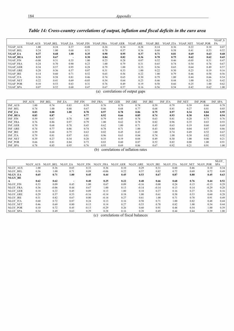
184 Appendix
Table 14: Cross-country correlations of output, inflation and fiscal deficits in the euro area
YGAP_AUS YGAP_BEL YGAP_EA YGAP_FIN YGAP_FRA YGAP_GER YGAP_GRE YGAP_IRE YGAP_ITA YGAP_NET YGAP_POR YGAP_SPA
YGAP_AUS 1.00 0.24 0.37 -0.08 0.24 0.34 0.28 0.14 0.36 0.22 0.10 0.07YGAP_BEL 0.24 1.00 0.68 0.31 0.70 0.57 0.36 0.60 0.58 0.41 0.53 0.52YGAP_EA 0.37 0.68 1.00 0.35 0.90 0.95 0.37 0.71 0.81 0.69 0.63 0.68YGAP_REA 0.33 0.67 - 0.30 0.84 0.82 0.36 0.70 0.75 0.62 0.62 0.65YGAP_FIN -0.08 0.31 0.35 1.00 0.23 0.28 0.07 0.52 0.46 -0.05 0.31 0.47YGAP_FRA 0.24 0.70 0.90 0.23 1.00 0.79 0.31 0.65 0.74 0.54 0.76 0.67YGAP_GER 0.34 0.57 0.95 0.28 0.79 1.00 0.33 0.56 0.65 0.64 0.49 0.57YGAP_GRE 0.28 0.36 0.37 0.07 0.31 0.33 1.00 0.22 0.30 0.23 0.19 0.16YGAP_IRE 0.14 0.60 0.71 0.52 0.65 0.56 0.22 1.00 0.79 0.46 0.58 0.56YGAP_ITA 0.36 0.58 0.81 0.46 0.74 0.65 0.30 0.79 1.00 0.44 0.66 0.54YGAP_NET 0.22 0.41 0.69 -0.05 0.54 0.64 0.23 0.46 0.44 1.00 0.25 0.42YGAP_POR 0.10 0.53 0.63 0.31 0.76 0.49 0.19 0.58 0.66 0.25 1.00 0.62YGAP_SPA 0.07 0.52 0.68 0.47 0.67 0.57 0.16 0.56 0.54 0.42 0.62 1.00
(a) correlations of output gaps
INF_AUS INF_BEL INF_EA INF_FIN INF_FRA INF_GER INF_GRE INF_IRE INF_ITA INF_NET INF_POR INF_SPA INF_AUS 1.00 0.74 0.83 0.59 0.76 0.70 0.74 0.59 0.79 0.39 0.66 0.78INF_BEL 0.74 1.00 0.88 0.67 0.86 0.68 0.77 0.68 0.81 0.27 0.81 0.85INF_EA 0.83 0.88 1.00 0.78 0.97 0.78 0.86 0.75 0.97 0.34 0.84 0.95INF_REA 0.83 0.87 - 0.77 0.92 0.66 0.85 0.74 0.93 0.30 0.84 0.94INF_FIN 0.59 0.67 0.78 1.00 0.79 0.45 0.74 0.63 0.81 0.20 0.73 0.76INF_FRA 0.76 0.86 0.97 0.79 1.00 0.62 0.78 0.82 0.96 0.35 0.83 0.93INF_GER 0.70 0.68 0.78 0.45 0.62 1.00 0.71 0.45 0.63 0.19 0.60 0.69INF_GRE 0.74 0.77 0.86 0.74 0.78 0.71 1.00 0.43 0.84 0.04 0.87 0.86INF_IRE 0.59 0.68 0.75 0.63 0.82 0.45 0.43 1.00 0.74 0.49 0.52 0.67INF_ITA 0.79 0.81 0.97 0.81 0.96 0.63 0.84 0.74 1.00 0.30 0.82 0.92INF_NET 0.39 0.27 0.34 0.20 0.35 0.19 0.04 0.49 0.30 1.00 0.00 0.21INF_POR 0.66 0.81 0.84 0.73 0.83 0.60 0.87 0.52 0.82 0.00 1.00 0.91INF_SPA 0.78 0.85 0.95 0.76 0.93 0.69 0.86 0.67 0.92 0.21 0.91 1.00
(b) correlations of inflation rates
NLGY_AUS NLGY_BEL NLGY_EA NLGY_FIN NLGY_FRA NLGY_GER NLGY_GRE NLGY_IRE NLGY_ITA NLGY_NET NLGY_POR NLGY_SPA
NLGY_AUS 1.00 0.36 0.65 0.33 0.36 0.10 0.29 0.31 0.60 0.46 0.10 0.34NLGY_BEL 0.36 1.00 0.71 0.09 -0.06 0.22 0.57 0.82 0.72 0.69 0.72 0.49NLGY_EA 0.65 0.71 1.00 0.45 0.44 0.45 0.53 0.67 0.87 0.80 0.45 0.63NLGY_REA 0.62 0.62 - 0.40 0.25 0.22 0.48 0.66 0.68 0.76 0.44 0.52NLGY_FIN 0.33 0.09 0.45 1.00 0.67 0.09 -0.16 0.00 0.24 0.15 -0.13 0.29NLGY_FRA 0.36 -0.06 0.44 0.67 1.00 0.13 -0.14 -0.14 0.13 0.14 -0.29 0.28NLGY_GER 0.10 0.22 0.45 0.09 0.13 1.00 0.18 0.27 0.16 0.27 0.26 0.16NLGY_GRE 0.29 0.57 0.53 -0.16 -0.14 0.18 1.00 0.61 0.58 0.53 0.60 0.28NLGY_IRE 0.31 0.82 0.67 0.00 -0.14 0.27 0.61 1.00 0.71 0.78 0.91 0.49NLGY_ITA 0.60 0.72 0.87 0.24 0.13 0.16 0.58 0.71 1.00 0.82 0.48 0.44NLGY_NET 0.46 0.69 0.80 0.15 0.14 0.27 0.53 0.78 0.82 1.00 0.54 0.44NLGY_POR 0.10 0.72 0.45 -0.13 -0.29 0.26 0.60 0.91 0.48 0.54 1.00 0.39NLGY_SPA 0.34 0.49 0.63 0.29 0.28 0.16 0.28 0.49 0.44 0.44 0.39 1.00
(c) correlations of fiscal balances

Appendix 185
Appendix 1b: Spillover effects in VAR models (from chapter 3)
Figure 39: Spillover from the (rest of the) euro area on individual countries (Austria, Belgium, Finland, Greece, Ireland, the Netherlands, Portugal, Spain)
(a) Austria
-.2
.0
.2
.4
2 4 6 8 10 12 14 16
Response of YGAP_AUS to YGAPREA_AUS
-.4-.3-.2-.1.0.1.2.3
2 4 6 8 10 12 14 16
Response of YGAP_AUS to NLGYREA_AUS
-.2-.1.0.1.2.3.4.5
2 4 6 8 10 12 14 16
Response of YGAP_AUS to SIN_EA
-.4
-.2
.0
.2
.4
2 4 6 8 10 12 14 16
Response of YGAP_AUS to INFRE A_AUS
-.3
-.2-.1
.0
.1
.2
.3
2 4 6 8 10 12 14 16
Response of NLGY_AUS to YGAPREA_AUS
-.3-.2-.1.0.1.2.3.4.5
2 4 6 8 10 12 14 16
Response of NLGY_AUS to NLGYREA_AUS
-.4-.3-.2-.1.0.1.2.3.4
2 4 6 8 10 12 14 16
Response of NLGY_AUS to SIN_EA
-.3
-.2
-.1
.0
.1
.2
.3
2 4 6 8 10 12 14 16
Response of NLGY_AUS to INFREA_AUS
-.6
-.4
-.2
.0
.2
2 4 6 8 10 12 14 16
Response of CUAY_AUS to YGAPREA_AUS
-.4
-.2
.0
.2
2 4 6 8 10 12 14 16
Response of CUAY_AUS to NLGYREA_AUS
-.4
-.2
.0
.2
2 4 6 8 10 12 14 16
Response of CUAY_AUS to SIN_E A
-.2
.0
.2
.4
.6
2 4 6 8 10 12 14 16
Response of CUAY_AUS to INFREA_AUS
.00
.05
.10
.15
.20
.25
2 4 6 8 10 12 14 16
Response of INF_AUS to YGAPREA_AUS
-.1
.0
.1
.2
2 4 6 8 10 12 14 16
Response of INF_AUS to NLGYREA_AUS
.00
.05
.10
.15
.20
.25
2 4 6 8 10 12 14 16
Response of I NF_AUS to SI N_EA
-.2
-.1
.0
.1
.2
.3
2 4 6 8 10 12 14 16
Response of INF_AUS to INFREA_AUS
Response to Generalized One S.D. Innovations ± 2 S.E.

186 Appendix
(a) Austria (cont’d)
.0
.1
.2
.3
.4
.5
2 4 6 8 10 12 14 16
Response of YGAPREA_AUS to YGAPREA_AUS
-.1
.0
.1
.2
.3
2 4 6 8 10 12 14 16
Response of YGAPREA_AUS to NLGYREA_AUS
-.1
.0
.1
.2
.3
.4
2 4 6 8 10 12 14 16
Response of YGAPREA_AUS to SIN_EA
-.1
.0
.1
.2
.3
2 4 6 8 10 12 14 16
Response of YGAPREA_AUS to I NFREA_AUS
-.2
-.1
.0
.1
.2
2 4 6 8 10 12 14 16
Response of NLGYREA_AUS to YGAPREA_AUS
-.1.0
.1
.2
.3
.4
.5
2 4 6 8 10 12 14 16
Response of NLGYREA_AUS to NLGYREA_AUS
-.2
-.1
.0
.1
2 4 6 8 10 12 14 16
Response of NLGYREA_AUS to SIN_EA
-.3
-.2
-.1
.0
.1
2 4 6 8 10 12 14 16
Response of NLGYREA_AUS to INFREA_AUS
.0
.1
.2
.3
.4
.5
.6
2 4 6 8 10 12 14 16
Response of SIN_EA to YGAPREA_AUS
-.2-.1.0.1.2.3.4.5
2 4 6 8 10 12 14 16
Response of SIN_EA to NLGYRE A_AUS
.0
.1
.2
.3
.4
.5
.6
2 4 6 8 10 12 14 16
Response of SIN_EA to SIN_EA
.0
.1
.2
.3
.4
.5
.6
.7
2 4 6 8 10 12 14 16
Response of SIN_EA to INFREA_AUS
-.05
.00
.05
.10
.15
.20
.25
2 4 6 8 10 12 14 16
Response of INFREA_AUS to YGAPREA_AUS
-.1
.0
.1
.2
2 4 6 8 10 12 14 16
Response of INFREA_AUS to NLGYREA_AUS
.0
.1
.2
.3
2 4 6 8 10 12 14 16
Response of I NFREA_AUS to SIN_EA
.0
.1
.2
.3
.4
2 4 6 8 10 12 14 16
Response of INFREA_AUS to INFREA_AUS

Appendix 187
(b) Belgium
.0
.1
.2
.3
2 4 6 8 10 12 14 16
Response of YGAP_BEL to YGAPREA_BEL
-.2
-.1
.0
.1
.2
.3
2 4 6 8 10 12 14 16
Response of YGAP_BEL to NLGYRE A_BEL
-.1
.0
.1
.2
.3
2 4 6 8 10 12 14 16
Response of YGAP_BEL to SIN_EA
-.2
-.1
.0
.1
.2
.3
2 4 6 8 10 12 14 16
Response of YGAP_BEL to I NFREA_BEL
-0.4
0.0
0.4
0.8
2 4 6 8 10 12 14 16
Response of NLGY_BEL to YGAPREA_BEL
-.4
-.2
.0
.2
.4
.6
2 4 6 8 10 12 14 16
Response of NLGY_BEL to NLGYREA_BEL
-.6-.4
-.2
.0
.2
.4
.6
2 4 6 8 10 12 14 16
Response of NLGY_BEL to SIN_EA
-.6-.4
-.2.0
.2
.4
.6
2 4 6 8 10 12 14 16
Response of NLGY_BEL to INFREA_BEL
-.4
-.2
.0
.2
.4
2 4 6 8 10 12 14 16
Response of CUAY_BEL to YGAPREA_BEL
-.4-.3-.2-.1.0.1.2
2 4 6 8 10 12 14 16
Response of CUAY_BEL to NLGYREA_BEL
-.3
-.2
-.1
.0
.1
.2
2 4 6 8 10 12 14 16
Response of CUAY_BEL to SIN_EA
-.5
-.4
-.3
-.2
-.1
.0
.1
2 4 6 8 10 12 14 16
Response of CUAY_BEL to INFREA_BEL
-.2
-.1
.0
.1
2 4 6 8 10 12 14 16
Response of INF_BEL to YGAPREA_BEL
-.1
.0
.1
.2
2 4 6 8 10 12 14 16
Response of INF_BEL to NLGYREA_BE L
-.1
.0
.1
.2
2 4 6 8 10 12 14 16
Response of INF_BEL to SIN_EA
.00
.04
.08
.12
.16
.20
.24
.28
2 4 6 8 10 12 14 16
Response of INF_BEL to INFREA_BEL
Response to Generalized One S. D. Innovations ± 2 S.E.
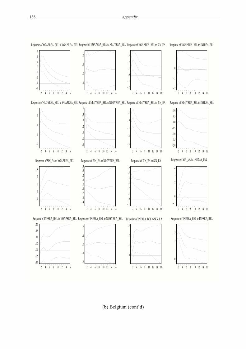
188 Appendix
(b) Belgium (cont’d)
-.1.0.1.2.3.4.5.6
2 4 6 8 10 12 14 16
Response of YGAPREA_BEL to YGAPREA_BEL
-.1
.0
.1
.2
2 4 6 8 10 12 14 16
Response of YGAPREA_BEL to NLGYREA_BEL
-.2
-.1
.0
.1
.2
.3
2 4 6 8 10 12 14 16
Response of YGAPREA_BEL to SIN_EA
-.2
-.1
.0
.1
2 4 6 8 10 12 14 16
Response of YGAPREA_BEL to INFREA_BEL
-.2
-.1
.0
.1
2 4 6 8 10 12 14 16
Response of NLGYREA_BEL to YGAPREA_BEL
-.1
.0
.1
.2
.3
.4
.5
2 4 6 8 10 12 14 16
Response of NLGYREA_BEL to NLGYREA_BEL
-.3
-.2
-.1
.0
.1
2 4 6 8 10 12 14 16
Response of NLGYREA_BEL to SIN_EA
-.20
-.15
-.10
-.05
.00
.05
.10
2 4 6 8 10 12 14 16
Response of NLGYREA_BEL to INFREA_BEL
.0
.1
.2
.3
.4
2 4 6 8 10 12 14 16
Response of SIN_EA to YGAPREA_BEL
-.4-.3-.2-.1.0.1.2.3.4
2 4 6 8 10 12 14 16
Response of SIN_EA to NLGYREA_BEL
-.1.0.1.2.3.4.5.6
2 4 6 8 10 12 14 16
Response of SIN_EA to SIN_EA
-.1
.0
.1
.2
.3
.4
2 4 6 8 10 12 14 16
Response of SIN_EA to I NFREA_BEL
-.10
-.05
.00
.05
.10
.15
.20
2 4 6 8 10 12 14 16
Response of INFREA_BE L to YGAPREA_BEL
-.2
-.1
.0
.1
.2
2 4 6 8 10 12 14 16
Response of INFREA_BEL to NLGYRE A_BEL
.0
.1
.2
.3
2 4 6 8 10 12 14 16
Response of INFREA_BEL to SI N_E A
.0
.1
.2
.3
2 4 6 8 10 12 14 16
Response of INFREA_BEL to INFRE A_BEL

Appendix 189
(c) Finland
-.8
-.6
-.4
-.2
.0
.2
2 4 6 8 10 12 14 16
Response of YGAP_FIN to YGAPREA_FIN
-.4
.0
.4
.8
2 4 6 8 10 12 14 16
Response of YGAP_FIN to NLGYREA_FIN
-.6
-.4
-.2
.0
.2
.4
2 4 6 8 10 12 14 16
Response of YGAP_FIN to SI N_E A
-.2
.0
.2
.4
.6
.8
2 4 6 8 10 12 14 16
Response of YGAP_FIN to INFREA_FIN
-.8
-.6
-.4
-.2
.0
.2
2 4 6 8 10 12 14 16
Response of NLGY_FIN to YGAPREA_FI N
-.4
.0
.4
.8
2 4 6 8 10 12 14 16
Response of NLGY_FIN to NLGYREA_FIN
-.8-.6
-.4-.2.0
.2
.4
2 4 6 8 10 12 14 16
Response of NLGY_FIN to SIN_EA
-0.4
0.0
0.4
0.8
2 4 6 8 10 12 14 16
Response of NLGY_FIN to INFREA_FIN
-.3-.2-.1.0.1.2.3.4
2 4 6 8 10 12 14 16
Response of CUAY_FIN to YGAPREA_FIN
-.2
.0
.2
.4
.6
2 4 6 8 10 12 14 16
Response of CUAY_FIN to NLGYREA_FIN
-.4-.3-.2-.1.0.1.2.3
2 4 6 8 10 12 14 16
Response of CUAY_FIN to SIN_EA
-.4
-.2
.0
.2
.4
2 4 6 8 10 12 14 16
Response of CUAY_FIN to INFREA_FIN
-.4
-.2
.0
.2
.4
2 4 6 8 10 12 14 16
Response of INF_FIN to YGAPREA_FIN
-.2
.0
.2
.4
.6
2 4 6 8 10 12 14 16
Response of INF_FIN to NLGYREA_FIN
-.4
-.2
.0
.2
.4
2 4 6 8 10 12 14 16
Response of INF_FIN to SIN_EA
-.2-.1.0.1.2.3.4.5
2 4 6 8 10 12 14 16
Response of INF_FIN to INFRE A_FI N
Response to Generalized One S. D. Innovations ± 2 S.E.

190 Appendix
(c) Finland (cont’d)
-.1.0.1.2.3.4.5.6
2 4 6 8 10 12 14 16
Response of YGAPREA_FIN to YGAPREA_FI N
-.2
-.1
.0
.1
.2
.3
2 4 6 8 10 12 14 16
Response of YGAPREA_FIN to NLGYREA_FIN
-.2
-.1
.0
.1
.2
.3
2 4 6 8 10 12 14 16
Response of YGAPREA_FIN to SIN_EA
-.2
-.1
.0
.1
.2
2 4 6 8 10 12 14 16
Response of YGAPREA_FIN to INFREA_FIN
-.08-.04.00
.04
.08
.12
.16
2 4 6 8 10 12 14 16
Response of NLGYREA_FIN to YGAPREA_FIN
-.1
.0
.1
.2
.3
.4
.5
2 4 6 8 10 12 14 16
Response of NLGYREA_FIN to NLGYREA_FIN
-.1
.0
.1
.2
2 4 6 8 10 12 14 16
Response of NLGYREA_FIN to SIN_EA
-.15
-.10
-.05
.00
.05
.10
2 4 6 8 10 12 14 16
Response of NLGYREA_FIN to INFREA_FIN
-.1
.0
.1
.2
2 4 6 8 10 12 14 16
Response of SIN_EA to YGAPREA_FIN
-.3
-.2
-.1
.0
.1
.2
.3
2 4 6 8 10 12 14 16
Response of SIN_EA to NLGYREA_FIN
-.1
.0
.1
.2
.3
.4
2 4 6 8 10 12 14 16
Response of SIN_EA to SIN_EA
-.1
.0
.1
.2
.3
2 4 6 8 10 12 14 16
Response of SIN_EA to INFREA_FIN
-.10
-.05
.00
.05
.10
2 4 6 8 10 12 14 16
Response of INFREA_FIN to YGAPREA_FIN
-.1
.0
.1
.2
2 4 6 8 10 12 14 16
Response of INFREA_FIN to NLGYRE A_FIN
.0
.1
.2
2 4 6 8 10 12 14 16
Response of INFREA_FIN to SIN_EA
.0
.1
.2
.3
2 4 6 8 10 12 14 16
Response of INFREA_FIN to INFREA_FIN

Appendix 191
(d) Greece
-.4
-.2
.0
.2
.4
2 4 6 8 10 12 14 16
Response of YGAP_GRE to YGAPREA_GRE
-.4
-.2
.0
.2
.4
2 4 6 8 10 12 14 16
Response of YGAP_GRE to NLGYREA_GRE
-.4
-.2
.0
.2
.4
2 4 6 8 10 12 14 16
Response of YGAP_GRE to SIN_EA
-.4
-.2
.0
.2
.4
.6
2 4 6 8 10 12 14 16
Response of YGAP_GRE to INFREA_GRE
-2
-1
0
1
2
2 4 6 8 10 12 14 16
Response of NLGY_GRE to YGAPREA_GRE
-2
-1
0
1
2
2 4 6 8 10 12 14 16
Response of NLGY_GRE to NLGYREA_GRE
-2
-1
0
1
2
2 4 6 8 10 12 14 16
Response of NLGY_GRE to SIN_EA
-3
-2
-1
0
1
2 4 6 8 10 12 14 16
Response of NLGY_GRE to INFREA_GRE
-.6
-.4
-.2
.0
.2
.4
2 4 6 8 10 12 14 16
Response of CUAY_GRE to YGAPREA_GRE
-.6
-.4
-.2
.0
.2
.4
2 4 6 8 10 12 14 16
Response of CUAY_GRE to NLGYREA_GRE
-.6
-.4
-.2
.0
.2
.4
2 4 6 8 10 12 14 16
Response of CUAY_GRE to SIN_EA
-.2
.0
.2
.4
.6
2 4 6 8 10 12 14 16
Response of CUAY_GRE to INFREA_GRE
-0.2
0.00.2
0.40.6
0.81.0
2 4 6 8 10 12 14 16
Response of INF_GRE to YGAPREA_GRE
-.6-.4-.2.0.2.4.6.8
2 4 6 8 10 12 14 16
Response of INF_GRE to NLGYREA_GRE
-0.4
0.0
0.4
0.8
1.2
2 4 6 8 10 12 14 16
Response of INF_GRE to SIN_EA
-0.20.00.20.40.60.81.01.2
2 4 6 8 10 12 14 16
Response of INF_GRE to INFREA_GRE
Response to Generalized O ne S.D. Innovations ± 2 S .E.
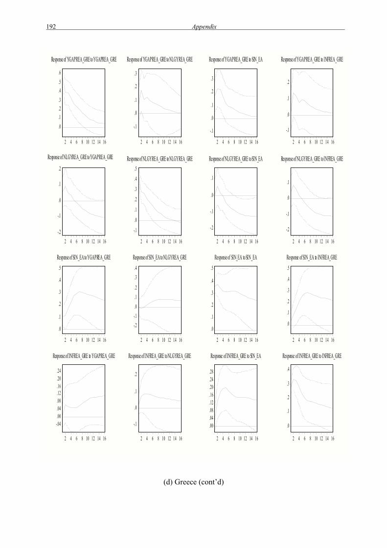
192 Appendix
(d) Greece (cont’d)
.0
.1
.2
.3
.4
.5
.6
2 4 6 8 10 12 14 16
Response of YGAPREA_GRE to YGAPREA_GRE
-.1
.0
.1
.2
.3
2 4 6 8 10 12 14 16
Response of YGAPREA_GRE to NLGYREA_GRE
-.1
.0
.1
.2
.3
2 4 6 8 10 12 14 16
Response of YGAPREA_GRE to SIN_EA
-.1
.0
.1
.2
2 4 6 8 10 12 14 16
Response of YGAPREA_GRE to INFREA_GRE
-.2
-.1
.0
.1
.2
2 4 6 8 10 12 14 16
Response of NLGYREA_GRE to YGAPREA_GRE
-.1
.0
.1
.2
.3
.4
.5
2 4 6 8 10 12 14 16
Response of NLGYREA_GRE to NLGYREA_GRE
-.2
-.1
.0
.1
2 4 6 8 10 12 14 16
Response of NLGYREA_GRE to SIN_EA
-.2
-.1
.0
.1
2 4 6 8 10 12 14 16
Response of NLGYREA_GRE to INFREA_GRE
.0
.1
.2
.3
.4
.5
2 4 6 8 10 12 14 16
Response of SIN_EA to YGAPREA_GRE
-.2-.1.0.1.2
.3
.4
2 4 6 8 10 12 14 16
Response of SIN_EA to NLGYREA_GRE
.0
.1
.2
.3
.4
.5
2 4 6 8 10 12 14 16
Response of SIN_EA to SIN_EA
.0
.1
.2
.3
.4
.5
2 4 6 8 10 12 14 16
Response of SIN_EA to INFREA_GRE
-.04.00.04.08.12.16.20.24
2 4 6 8 10 12 14 16
Response of INFREA_GRE to YGAPREA_GRE
-.1
.0
.1
.2
2 4 6 8 10 12 14 16
Response of INFREA_GRE to NLGYREA_GRE
.00
.04
.08
.12
.16
.20
.24
.28
2 4 6 8 10 12 14 16
Response of INFREA_GRE to SIN_EA
.0
.1
.2
.3
.4
2 4 6 8 10 12 14 16
Response of INFREA_GRE to INFREA_GRE

Appendix 193
(e) Ireland
-.2
.0
.2
.4
2 4 6 8 10 12 14 16
Response of YGAP_IRE to YGAPREA_IRE
-.2
-.1
.0
.1
.2
.3
2 4 6 8 10 12 14 16
Response of YGAP_IRE to NLGYREA_I RE
-.4-.3-.2-.1.0.1.2.3
2 4 6 8 10 12 14 16
Response of YGAP_IRE to SIN_EA
-.3-.2-.1
.0
.1
.2
.3
2 4 6 8 10 12 14 16
Response of YGAP_IRE to INFREA_IRE
-.6
-.4
-.2
.0
.2
2 4 6 8 10 12 14 16
Response of NLGY_IRE to YGAPREA_IRE
-.6-.5-.4-.3-.2-.1.0.1
2 4 6 8 10 12 14 16
Response of NLGY_IRE to NLGYREA_IRE
-.8
-.6
-.4
-.2
.0
2 4 6 8 10 12 14 16
Response of NLGY_IRE to SIN_EA
-.6-.5-.4-.3-.2-.1.0.1
2 4 6 8 10 12 14 16
Response of NLGY_IRE to I NFREA_IRE
-.6
-.4
-.2
.0
.2
2 4 6 8 10 12 14 16
Response of CUAY_IRE to YGAPRE A_IRE
-.6-.4-.2.0
.2
.4
.6
2 4 6 8 10 12 14 16
Response of CUAY_IRE to NLGYREA_IRE
-.4
-.2
.0
.2
.4
2 4 6 8 10 12 14 16
Response of CUAY_IRE to SIN_EA
-.8
-.4
.0
.4
2 4 6 8 10 12 14 16
Response of CUAY_IRE to INFREA_IRE
-.6-.5-.4-.3-.2-.1.0.1.2
2 4 6 8 10 12 14 16
Response of INF_IRE to YGAPREA_IRE
-.2
.0
.2
.4
.6
2 4 6 8 10 12 14 16
Response of INF_IRE to NLGYREA_IRE
-.4
-.2
.0
.2
.4
.6
2 4 6 8 10 12 14 16
Response of INF_IRE to SIN_EA
-.4
-.2
.0
.2
.4
.6
2 4 6 8 10 12 14 16
Response of INF_I RE to INFREA_IRE
Response to Generalized One S.D. Innovations ± 2 S.E.

194 Appendix
(e) Ireland (cont’d)
-.1.0.1.2.3.4.5.6
2 4 6 8 10 12 14 16
Response of YGAPREA_IRE to YGAPREA_IRE
-.2
-.1
.0
.1
.2
2 4 6 8 10 12 14 16
Response of YGAPREA_IRE to NL GYREA_IRE
-.2
-.1
.0
.1
.2
.3
.4
2 4 6 8 10 12 14 16
Response of YGAPREA_IRE to SIN_EA
-.1
.0
.1
.2
2 4 6 8 10 12 14 16
Response of YGAPREA_IRE to INFREA_I RE
-.2
-.1
.0
.1
2 4 6 8 10 12 14 16
Response of NLGYREA_IRE to YGAPREA_IRE
-.1
.0
.1
.2
.3
.4
2 4 6 8 10 12 14 16
Response of NLGYREA_IRE to NLGYREA_IRE
-.3
-.2
-.1
.0
.1
2 4 6 8 10 12 14 16
Response of NLGYREA_IRE to SIN_EA
-.20
-.15
-.10
-.05
.00
.05
2 4 6 8 10 12 14 16
Response of NLGYRE A_IRE to INFREA_IRE
.0
.1
.2
.3
.4
.5
.6
2 4 6 8 10 12 14 16
Response of SIN_EA to YGAPREA_IRE
-.2
-.1
.0
.1
.2
.3
2 4 6 8 10 12 14 16
Response of SIN_EA to NLGYREA_IRE
-.1.0.1.2.3.4.5.6
2 4 6 8 10 12 14 16
Response of SIN_EA to SIN_EA
-.1.0
.1
.2
.3
.4
.5
2 4 6 8 10 12 14 16
Response of SIN_EA to I NFREA_IRE
-.04.00.04.08.12.16.20.24
2 4 6 8 10 12 14 16
Response of INFREA_IRE to YGAPREA_IRE
-.08-.04.00.04.08.12.16
2 4 6 8 10 12 14 16
Response of INFREA_IRE to NLGYREA_I RE
.00
.05
.10
.15
.20
.25
2 4 6 8 10 12 14 16
Response of INFREA_IRE to SIN_EA
.0
.1
.2
.3
2 4 6 8 10 12 14 16
Response of INFREA_IRE to INFREA_IRE

Appendix 195
(f) Netherlands
-.4
-.2
.0
.2
.4
2 4 6 8 10 12 14 16
Response of YGAP_NET to YGAPREA_NET
-.3-.2-.1.0.1.2.3.4
2 4 6 8 10 12 14 16
Response of YGAP_NET to NLGYREA_NET
-.3-.2-.1.0.1.2.3
2 4 6 8 10 12 14 16
Response of YGAP_NET to SIN_EA
-.2
-.1
.0
.1
.2
2 4 6 8 10 12 14 16
Response of YGAP_NET to INFREA_NET
-.4
-.3
-.2
-.1
.0
.1
2 4 6 8 10 12 14 16
Response of NLGY_NET to YGAPREA_NET
-.3-.2-.1.0.1.2.3.4
2 4 6 8 10 12 14 16
Response of NLGY_NET to NLGYREA_NET
-.4
-.3
-.2
-.1
.0
.1
2 4 6 8 10 12 14 16
Response of NLGY_NET to SIN_EA
-.3
-.2
-.1
.0
.1
.2
2 4 6 8 10 12 14 16
Response of NLGY_NET to INFREA_NET
-.4
-.2
.0
.2
.4
2 4 6 8 10 12 14 16
Response of CUAY_NET to YGAPREA_NET
-.4
-.2
.0
.2
.4
2 4 6 8 10 12 14 16
Response of CUAY_NET to NLGYREA_NET
-.4
-.3-.2
-.1.0
.1
.2
2 4 6 8 10 12 14 16
Response of CUAY_NET to SI N_EA
-.4
-.2
.0
.2
.4
2 4 6 8 10 12 14 16
Response of CUAY_NET to INFREA_NE T
-.1
.0
.1
.2
.3
2 4 6 8 10 12 14 16
Response of INF_NET to YGAPREA_NET
-.1
.0
.1
.2
.3
2 4 6 8 10 12 14 16
Response of INF_NET to NLGYREA_NET
-.2
-.1.0
.1
.2
.3
.4
2 4 6 8 10 12 14 16
Response of INF_NET to SIN_EA
-.3
-.2
-.1
.0
.1
2 4 6 8 10 12 14 16
Response of INF_NET to I NFREA_NET
Response to Generalized One S.D. Innovations ± 2 S.E.

196 Appendix
(f) Netherlands (cont’d)
-.1.0.1.2.3.4.5.6
2 4 6 8 10 12 14 16
Response of YGAPREA_NET to YGAPREA_NET
-.2
-.1
.0
.1
.2
.3
2 4 6 8 10 12 14 16
Response of YGAPREA_NET to NLGYREA_NET
-.1
.0
.1
.2
.3
2 4 6 8 10 12 14 16
Response of YGAPREA_NET to SIN_EA
-.1
.0
.1
.2
2 4 6 8 10 12 14 16
Response of YGAPREA_NE T to INFREA_NET
-.3
-.2
-.1
.0
.1
.2
2 4 6 8 10 12 14 16
Response of NLGYREA_NET to YGAPREA_NET
-.1
.0
.1
.2
.3
.4
.5
2 4 6 8 10 12 14 16
Response of NLGYREA_NET to NLGYREA_NET
-.2
-.1
.0
.1
2 4 6 8 10 12 14 16
Response of NLGYREA_NET to SIN_EA
-.15
-.10-.05
.00
.05
.10
2 4 6 8 10 12 14 16
Response of NLGYREA_NET to INFREA_NET
.0
.1
.2
.3
.4
.5
.6
.7
2 4 6 8 10 12 14 16
Response of SI N_EA to YGAPREA_NET
-.4
-.2
.0
.2
.4
2 4 6 8 10 12 14 16
Response of SIN_E A to NLGYREA_NET
-.1.0.1.2.3.4.5.6
2 4 6 8 10 12 14 16
Response of SIN_EA to SIN_EA
-.1
.0
.1
.2
.3
.4
.5
2 4 6 8 10 12 14 16
Response of SIN_EA to INFREA_NET
.0
.1
.2
.3
.4
2 4 6 8 10 12 14 16
Response of INFREA_NET to YGAPREA_NET
-.2
-.1
.0
.1
.2
.3
2 4 6 8 10 12 14 16
Response of INFREA_NET to NLGYREA_NET
.0
.1
.2
.3
2 4 6 8 10 12 14 16
Response of INFREA_NET to SIN_EA
.0
.1
.2
.3
2 4 6 8 10 12 14 16
Response of INFREA_NET to I NFREA_NET

Appendix 197
(g) Portugal
-.2-.1.0.1.2.3.4.5.6
2 4 6 8 10 12 14 16
Response of YGAP_POR to YGAPREA_POR
-.1
.0
.1
.2
.3
.4
2 4 6 8 10 12 14 16
Response of YGAP_POR to NLGYREA_POR
-.3
-.2
-.1
.0
.1
.2
2 4 6 8 10 12 14 16
Response of YGAP_POR to SIN_EA
-.4
-.3
-.2
-.1
.0
.1
.2
2 4 6 8 10 12 14 16
Response of YGAP_POR to INFREA_POR
-.4
-.2
.0
.2
.4
.6
2 4 6 8 10 12 14 16
Response of NLGY_POR to YGAPREA_POR
-.5-.4-.3-.2-.1.0.1.2.3
2 4 6 8 10 12 14 16
Response of NLGY_POR to NLGYREA_POR
-.5-.4-.3-.2-.1.0.1.2
2 4 6 8 10 12 14 16
Response of NLGY_POR to SIN_EA
-.4
-.2
.0
.2
.4
2 4 6 8 10 12 14 16
Response of NLGY_POR to INFREA_POR
-.2
.0
.2
.4
.6
2 4 6 8 10 12 14 16
Response of CUAY_POR to YGAPREA_POR
-.4
.0
.4
2 4 6 8 10 12 14 16
Response of CUAY_POR to NLGYREA_POR
-.6
-.4
-.2
.0
.2
.4
2 4 6 8 10 12 14 16
Response of CUAY_POR to SIN_EA
-.8
-.4
.0
.4
2 4 6 8 10 12 14 16
Response of CUAY_POR to INFREA_POR
-.6
-.4
-.2
.0
.2
.4
2 4 6 8 10 12 14 16
Response of INF_POR to YGAPREA_POR
-.2
.0
.2
.4
.6
.8
2 4 6 8 10 12 14 16
Response of INF_POR to NLGYREA_POR
-.4
-.2
.0
.2
.4
2 4 6 8 10 12 14 16
Response of INF_POR to SIN_EA
-.8-.6
-.4
-.2
.0
.2
.4
2 4 6 8 10 12 14 16
Response of INF_POR to INFREA_POR
Response to G eneralized One S.D. Innovation s ± 2 S .E.

198 Appendix
(g) Portugal (cont’d)
-.1.0.1.2.3.4.5.6
2 4 6 8 10 12 14 16
Response of YGAPREA_POR to YGAPREA_POR
-.1
.0
.1
.2
2 4 6 8 10 12 14 16
Response of YGAPREA_POR to NLGYREA_POR
-.2
-.1
.0
.1
.2
.3
2 4 6 8 10 12 14 16
Response of YGAPREA_POR to SIN_EA
-.2
-.1
.0
.1
2 4 6 8 10 12 14 16
Response of YGAPREA_POR to INFREA_POR
-.2
-.1
.0
.1
2 4 6 8 10 12 14 16
Response of NLGYREA_POR to YGAPREA_POR
-.1
.0
.1
.2
.3
.4
2 4 6 8 10 12 14 16
Response of NLGYREA_POR to NLGYREA_POR
-.20
-.15
-.10-.05
.00
.05
2 4 6 8 10 12 14 16
Response of NLGYREA_POR to SIN_EA
-.2
-.1
.0
.1
2 4 6 8 10 12 14 16
Response of NLGYREA_POR to INFREA_POR
.0
.1
.2
.3
.4
.5
2 4 6 8 10 12 14 16
Response of SIN_EA to YGAPREA_POR
-.2-.1.0.1.2.3.4
2 4 6 8 10 12 14 16
Response of SIN_EA to NLGYREA_POR
-.1.0
.1
.2
.3
.4
.5
2 4 6 8 10 12 14 16
Response of SIN_EA to SIN_EA
-.4
-.3-.2
-.1
.0
.1
.2
2 4 6 8 10 12 14 16
Response of SIN_EA to INFREA_POR
-.05
.00
.05
.10
.15
.20
2 4 6 8 10 12 14 16
Response of INFREA_POR to YGAPREA_POR
-.15-.10-.05
.00
.05
.10
.15
2 4 6 8 10 12 14 16
Response of INFREA_POR to NLGYREA_POR
.00
.05
.10
.15
.20
2 4 6 8 10 12 14 16
Response of INFREA_POR to SIN_EA
-.1
.0
.1
.2
2 4 6 8 10 12 14 16
Response of INFREA_POR to INFREA_POR

Appendix 199
(h) Spain
.0
.1
.2
2 4 6 8 10 12 14 16
Response of YGAP_SPA to YGAPREA_SPA
-.1
.0
.1
.2
2 4 6 8 10 12 14 16
Response of YGAP_SPA to NLGYREA_SPA
-.20
-.15
-.10
-.05
.00
.05
2 4 6 8 10 12 14 16
Response of YGAP_SPA to SIN_EA
-.1
.0
.1
.2
2 4 6 8 10 12 14 16
Response of YGAP_SPA to INFREA_SPA
-.5
.0
.5
2 4 6 8 10 12 14 16
Response of NLGY_SPA to YGAPREA_SPA
-.4
.0
.4
2 4 6 8 10 12 14 16
Response of NLGY_SPA to NLGYREA_SPA
-.8
-.4
.0
.4
2 4 6 8 10 12 14 16
Response of NLGY_SP A to SIN_EA
-.6
-.4
-.2
.0
.2
.4
.6
2 4 6 8 10 12 14 16
Response of NLGY_SPA to INFREA_SPA
-.3
-.2
-.1
.0
2 4 6 8 10 12 14 16
Response of CUAY_SPA to YGAPREA_SPA
-.3
-.2
-.1
.0
.1
.2
2 4 6 8 10 12 14 16
Response of CUAY_SPA to NLGYREA_SPA
-.1
.0
.1
.2
2 4 6 8 10 12 14 16
Response of CUAY_SP A to SIN_EA
-.3
-.2
-.1
.0
.1
.2
2 4 6 8 10 12 14 16
Response of CUAY_SPA to INFREA_SPA
-.3
-.2
-.1
.0
.1
.2
.3
2 4 6 8 10 12 14 16
Response of I NF_SPA to YGAPREA_SPA
-.2-.1.0.1.2.3.4
2 4 6 8 10 12 14 16
Response of INF_SPA to NLGYREA_SPA
-.1
.0
.1
.2
.3
2 4 6 8 10 12 14 16
Response of INF_SPA to SIN_E A
.0
.1
.2
.3
.4
.5
.6
2 4 6 8 10 12 14 16
Response of INF_SPA to INFREA_SPA
Response to Generalized One S.D. Innovations ± 2 S.E.

200 Appendix
(h) Spain (cont’d)
.0
.1
.2
.3
.4
.5
.6
2 4 6 8 10 12 14 16
Response of YGAPREA_SPA to YGAPREA_SPA
-.1
.0
.1
.2
2 4 6 8 10 12 14 16
Response of YGAPREA_SPA to NLGYREA_SPA
-.1
.0
.1
.2
2 4 6 8 10 12 14 16
Response of YGAPREA_SP A to SIN_EA
-.1
.0
.1
.2
2 4 6 8 10 12 14 16
Response of YGAPREA_SPA to INFREA_SPA
-.10
-.05
.00
.05
.10
.15
2 4 6 8 10 12 14 16
Response of NLGYREA_SPA to YGAPREA_SPA
-.1
.0
.1
.2
.3
.4
2 4 6 8 10 12 14 16
Response of NLGYREA_SPA to NLGYREA_SPA
-.15
-.10
-.05
.00
.05
2 4 6 8 10 12 14 16
Response of NLGYREA_SPA to SIN_EA
-.2
-.1
.0
.1
2 4 6 8 10 12 14 16
Response of NLGYREA_SPA to INFREA_SPA
-.1
.0
.1
.2
.3
.4
2 4 6 8 10 12 14 16
Response of SIN_EA to YGAPREA_SPA
-.3-.2-.1.0.1.2.3.4.5
2 4 6 8 10 12 14 16
Response of SIN_EA to NLGYRE A_SPA
-.2
-.1
.0
.1
.2
.3
.4
2 4 6 8 10 12 14 16
Response of SIN_EA to SIN_EA
.0
.1
.2
.3
.4
.5
.6
2 4 6 8 10 12 14 16
Response of SIN_EA to INFREA_SPA
-.1
.0
.1
2 4 6 8 10 12 14 16
Response of I NFREA_SPA to YGAP REA_SPA
-.1
.0
.1
.2
2 4 6 8 10 12 14 16
Response of INFREA_SPA to NLGYRE A_SPA
-.10
-.05
.00
.05
.10
.15
2 4 6 8 10 12 14 16
Response of INFREA_SPA to SIN_E A
.0
.1
.2
.3
2 4 6 8 10 12 14 16
Response of INFREA_SPA to INFREA_SPA

Appendix 201
Appendix 2a: Domestic economy: SVAR models with exogenous debt ratio.

202 Appendix
Figure 40: Domestic economy, SVAR-model (4.1a-b): impulse responses of real long-term interest rates to shocks of 1% of GDP in net lending ratio.
shock to net lending ratio shock to net lending ratio
Austria Belgium
-60
-40
-20
0
20
40
60
1 2 3 4 5 6 7 8 9 10
-15
-10
-5
0
5
10
15
20
25
30
35
40
1 2 3 4 5 6 7 8 9 10
Germany Finland
-40
-30
-20
-10
0
10
20
30
40
1 2 3 4 5 6 7 8 9 10
-50
-40
-30
-20
-10
0
10
20
30
40
50
1 2 3 4 5 6 7 8 9 10
France United Kingdom
-60
-40
-20
0
20
40
60
80
100
1 2 3 4 5 6 7 8 9 10
-30
-20
-10
0
10
20
30
40
1 2 3 4 5 6 7 8 9 10
Italy The Netherlands
-15
-10
-5
0
5
10
15
20
1 2 3 4 5 6 7 8 9 10
-10
0
10
20
30
40
50
60
70
80
90
100
1 2 3 4 5 6 7 8 9 10
euro area
-0.2
-0.1
0
0.1
0.2
0.3
0.4
1 2 3 4 5 6 7 8 9 10

Appendix 203
Appendix 2b: SVAR models with yield.
Figure 41: Domestic economy, SVAR-model (4.1a-b): impulse responses of yield to shocks of 1% of GDP in net lending and debt ratio
shock to net lending ratio shock to debt ratio
Austria
-0.6
-0.4
-0.2
0
0.2
0.4
0.6
0.8
1 2 3 4 5 6 7 8 9 10
-1.2
-1
-0.8
-0.6
-0.4
-0.2
0
0.2
0.4
0.6
1 2 3 4 5 6 7 8 9 10
Belgium
-0.6
-0.4
-0.2
0
0.2
0.4
0.6
0.8
1
1.2
1 2 3 4 5 6 7 8 9 10
-3.5
-3
-2.5
-2
-1.5
-1
-0.5
0
0.5
1
1 2 3 4 5 6 7 8 9 10
Germany
-0.8
-0.6
-0.4
-0.2
0
0.2
0.4
0.6
1 2 3 4 5 6 7 8 9 10
-0.8
-0.6
-0.4
-0.2
0
0.2
0.4
0.6
0.8
1
1.2
1 2 3 4 5 6 7 8 9 10
Finland
-0.5
-0.4
-0.3
-0.2
-0.1
0
0.1
0.2
0.3
0.4
0.5
1 2 3 4 5 6 7 8 9 10
-1.5
-1
-0.5
0
0.5
1
1.5
1 2 3 4 5 6 7 8 9 10

204 Appendix
shock to net lending ratio shock to debt ratio
France
-0.6
-0.4
-0.2
0
0.2
0.4
0.6
0.8
1
1.2
1 2 3 4 5 6 7 8 9 10
-2
-1.5
-1
-0.5
0
0.5
1 2 3 4 5 6 7 8 9 10
United Kingdom
-0.6
-0.4
-0.2
0
0.2
0.4
0.6
1 2 3 4 5 6 7 8 9 10
-1.5
-1
-0.5
0
0.5
1
1.5
1 2 3 4 5 6 7 8 9 10
Italy
-0.6
-0.4
-0.2
0
0.2
0.4
0.6
0.8
1 2 3 4 5 6 7 8 9 10
-1.5
-1
-0.5
0
0.5
1
1.5
1 2 3 4 5 6 7 8 9 10
The Netherlands
-0.8
-0.6
-0.4
-0.2
0
0.2
0.4
0.6
0.8
1
1.2
1 2 3 4 5 6 7 8 9 10
-2
-1.5
-1
-0.5
0
0.5
1
1 2 3 4 5 6 7 8 9 10
Notes: (a) graphs display percentage point impulse responses of the interest rate measure, in response to a shock; (b) 90% confidence intervals from bootstrapped model – with 1000 draws – are the average (normal continuous line) and maximum (bold continuous line) of all four Choleski orders.

Appendix 205
Figure 42: Euro area economy, SVAR-model (4.1a-b): impulse responses of yield to shocks
of 1% of GDP in net lending and debt ratio
shock to net lending ratio shock to debt ratio
-0.5
-0.4
-0.3
-0.2
-0.1
0
0.1
0.2
0.3
0.4
0.5
0.6
1 2 3 4 5 6 7 8 9 10
-0.04
-0.03
-0.02
-0.01
0
0.01
0.02
0.03
0.04
1 2 3 4 5 6 7 8 9 10
Notes: (a) graphs display percentage impulse responses of the interest rate measure, in response to a shock; (b) 90% confidence intervals from bootstrapped model – with 1000 draws – are the average (normal continuous line) and maximum (bold continuous line) of all four Choleski orders.

206 Appendix
Figure 43: Domestic economy, SVAR-model (4.1a-b): impulse responses of yield to shocks
of 1% of GDP in net lending ratio
shock to net lending ratio shock to net lending ratio Austria Belgium
-60
-40
-20
0
20
40
60
1 2 3 4 5 6 7 8 9 10
-35
-30
-25
-20
-15
-10
-5
0
5
10
1 2 3 4 5 6 7 8 9 10
Germany Finland
-40
-30
-20
-10
0
10
20
30
40
50
60
70
1 2 3 4 5 6 7 8 9 10
-30
-20
-10
0
10
20
30
40
50
1 2 3 4 5 6 7 8 9 10
France United Kingdom
-150
-100
-50
0
50
100
1 2 3 4 5 6 7 8 9 10
-30
-20
-10
0
10
20
30
40
1 2 3 4 5 6 7 8 9 10
Italy The Netherlands
-20
-15
-10
-5
0
5
10
15
1 2 3 4 5 6 7 8 9 10
-60
-50
-40
-30
-20
-10
0
10
20
1 2 3 4 5 6 7 8 9 10
euro area
-0.6
-0.4
-0.2
0
0.2
0.4
0.6
1 2 3 4 5 6 7 8 9 10

Appendix 207
Figure 44: Open economy, SVAR-model (4.2a): on difference of country i to euro area; impulse responses of yield to 1 standard deviation shocks in net lending and debt ratio
shock to net lending ratio shock to debt ratio
Austria
-0.6
-0.4
-0.2
0
0.2
0.4
0.6
0.8
1 2 3 4 5 6 7 8 9 10
-1.4
-1.2
-1
-0.8
-0.6
-0.4
-0.2
0
0.2
0.4
1 2 3 4 5 6 7 8 9 10
Belgium
-0.8
-0.6
-0.4
-0.2
0
0.2
0.4
0.6
1 2 3 4 5 6 7 8 9 10
-4
-3
-2
-1
0
1
2
3
4
1 2 3 4 5 6 7 8 9 10
Germany
-0.8
-0.6
-0.4
-0.2
0
0.2
0.4
0.6
0.8
1 2 3 4 5 6 7 8 9 10
-2
-1.5
-1
-0.5
0
0.5
1
1.5
1 2 3 4 5 6 7 8 9 10
Finland
-1
-0.8
-0.6
-0.4
-0.2
0
0.2
0.4
0.6
0.8
1 2 3 4 5 6 7 8 9 10
-1
-0.5
0
0.5
1
1.5
2
1 2 3 4 5 6 7 8 9 10
France
-0.5
-0.4
-0.3
-0.2
-0.1
0
0.1
0.2
0.3
0.4
0.5
0.6
1 2 3 4 5 6 7 8 9 10
-1.5
-1
-0.5
0
0.5
1
1 2 3 4 5 6 7 8 9 10

208 Appendix
shock to net lending ratio shock to debt ratio
Italy
-0.6
-0.4
-0.2
0
0.2
0.4
0.6
0.8
1 2 3 4 5 6 7 8 9 10
-1.5
-1
-0.5
0
0.5
1
1 2 3 4 5 6 7 8 9 10
The Netherlands
-0.4
-0.3
-0.2
-0.1
0
0.1
0.2
0.3
0.4
0.5
0.6
0.7
1 2 3 4 5 6 7 8 9 10
-1
-0.5
0
0.5
1
1.5
2
2.5
1 2 3 4 5 6 7 8 9 10
Notes: (a) graphs display percentage impulse responses of the interest rate measure, in response to a shock; (b) 90% confidence intervals from bootstrapped model – with 1000 draws – are the average (normal continuous line) and maximum (bold continuous line) of all four Choleski orders.

Appendix 209
Table 15: Domestic economy: forecast error variance decomposition of yield
horizon debt endogenous debt exogenous
country year debt deficit net lending
euro area 1 18.18 6.25 0.50 5 21.73 11.44 1.77 10 21.79 13.34 5.31
Germany 1 2.27 4.42 2.61 5 1.68 7.87 8.59 10 1.85 7.42 8.75
France 1 8.71 0.15 0.01 5 8.09 19.64 3.13 10 7.19 20.25 4.12
Italy 1 10.65 7.82 2.99 5 10.39 8.12 5.52 10 10.68 8.19 8.33
United Kingdom 1 39.28 1.98 1.98
5 35.38 6.34 9.25 10 32.53 6.30 9.87
Austria 1 7.35 4.36 1.06 5 19.58 23.36 12.50 10 18.99 23.43 14.83
Belgium 1 3.73 20.01 17.76 5 5.08 18.11 18.90 10 5.05 17.88 21.15
Finland 1 0.71 10.98 21.68 5 20.01 7.76 27.44 10 23.48 7.78 25.54
Netherlands 1 1.24 0.24 0.09 5 0.98 7.07 8.47 10 0.94 6.31 8.12

210 Appendix
Table 16: Open economy: forecast error variance decomposition of yield
horizon difference of country i to euro area
country year debt net lending
Germany 1 0.31 0.84 5 1.36 2.45 10 1.48 2.36
France 1 0.00 9.51 5 0.08 8.43 10 0.09 9.12
Italy 1 2.91 0.77 5 2.65 0.73 10 2.64 0.98
United Kingdom 1 0.70 24.51
5 2.18 28.06 10 1.99 31.94
Austria 1 0.05 0.08 5 11.18 0.37 10 14.00 1.15
Belgium 1 0.00 1.25 5 3.99 3.29 10 4.73 3.63
Finland 1 0.28 0.94 5 0.84 1.32 10 0.95 4.62
Netherlands 1 3.31 0.03 5 2.98 1.05 10 2.91 1.27
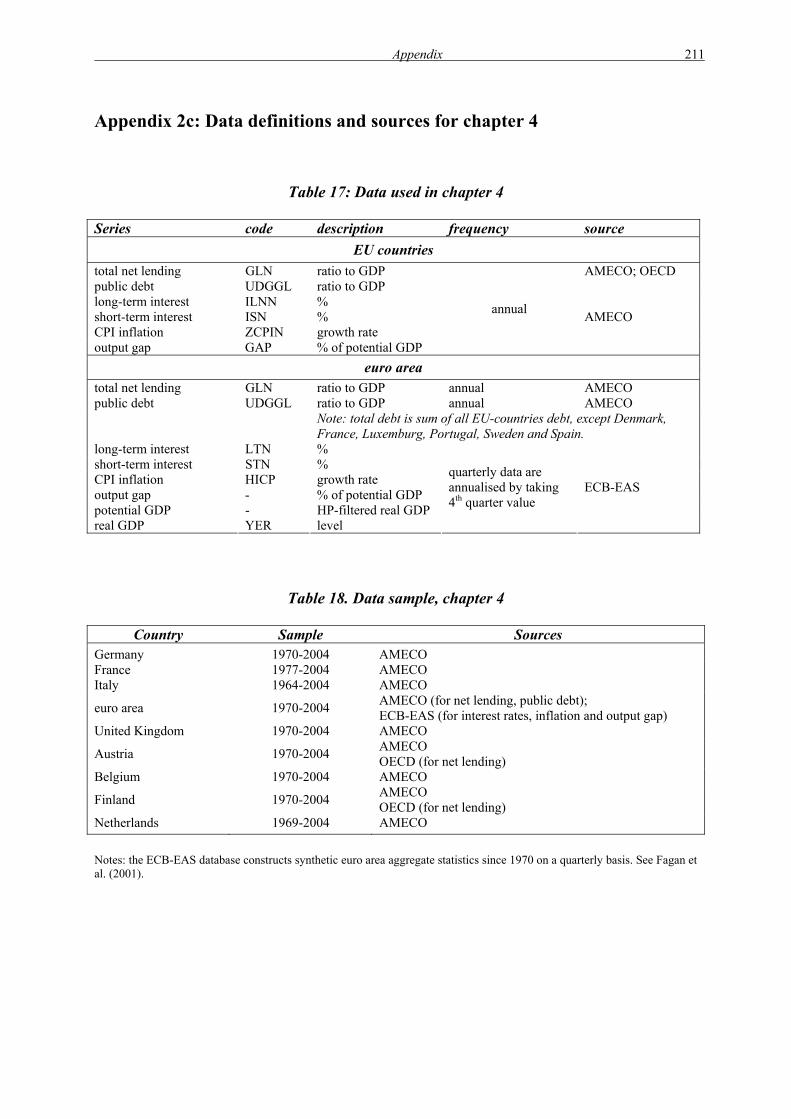
Appendix 211
Appendix 2c: Data definitions and sources for chapter 4
Table 17: Data used in chapter 4 Series code description frequency source
EU countries total net lending GLN ratio to GDP AMECO; OECD public debt UDGGL ratio to GDP long-term interest ILNN % short-term interest ISN % CPI inflation ZCPIN growth rate output gap GAP % of potential GDP
annual AMECO
euro area total net lending GLN ratio to GDP annual AMECO public debt UDGGL ratio to GDP annual AMECO Note: total debt is sum of all EU-countries debt, except Denmark,
France, Luxemburg, Portugal, Sweden and Spain. long-term interest LTN % short-term interest STN % CPI inflation HICP growth rate output gap - % of potential GDP potential GDP - HP-filtered real GDP real GDP YER level
quarterly data are annualised by taking 4th quarter value
ECB-EAS
Table 18. Data sample, chapter 4
Country Sample Sources Germany 1970-2004 AMECO France 1977-2004 AMECO Italy 1964-2004 AMECO
euro area 1970-2004 AMECO (for net lending, public debt); ECB-EAS (for interest rates, inflation and output gap)
United Kingdom 1970-2004 AMECO
Austria 1970-2004 AMECO OECD (for net lending)
Belgium 1970-2004 AMECO
Finland 1970-2004 AMECO OECD (for net lending)
Netherlands 1969-2004 AMECO
Notes: the ECB-EAS database constructs synthetic euro area aggregate statistics since 1970 on a quarterly basis. See Fagan et al. (2001).

212 Appendix
Appendix 3: The McKibbin-Sachs Global Model
The macroeconomic model simulations in this report use the MSG3 model, the most recent
version of the McKibbin-Sachs Global Model. This is a dynamic, intertemporal, general-
equilibrium model of a multi-region world economy. Based on microeconomic foundations
by assuming that economic agents maximise intertemporal objective functions, the model
exhibits a mixture of classical and Keynesian properties: partly rational expectations in
combination with various rigidities allow for deviations from fully optimising behaviour. In
particular, nominal wages are assumed to adjust slowly in the major industrial economies.
Nevertheless, the model solves for a full intertemporal equilibrium. McKibbin and Sachs
(1991) describe the original version of the model in full detail.
The MSG3 model is a two-sector version of the twelve-sector G-Cubed multi-country of
McKibbin and Wilcoxen (1998). In many ways the aggregation gives a model similar to the
McKibbin and Sachs (1991) MSG2 model except that there is substantial estimation of key
parameters in the MSG3 model. The two sectors of production are energy and non-energy.
There is also a third capital goods producing sector. MSG3 is therefore very similar in
sectoral and country coverage to the MSG2 model but includes many of the features of the
newer G-Cubed model. Overall, the model is designed to provide a bridge between
computable general equilibrium models and macroeconomic models by integrating the more
desirable features of both approaches. Details on this integration and how the G-cubed model
bridges the gap between CGE and traditional macroeconometric models can be found in
McKibbin and Wilcoxen (1998). Additional resources are available on the web
(http://www.msgpl.com.au/).
The main features of the new MSG3 model relative to the previous MSG2 model are:
• A better mapping of the energy flows in the economy based on country specific input-
output data from the G-Cubed database.
• Estimated production technologies based on the G-Cubed twelve-sector aggregation
are aggregated to the two-sector level, which gives a better depiction of the aggregate
production substitution possibilities than in the MSG2 model which assumed a Cobb-
Douglas specification.
• Explicit treatment of capital goods in the household and firm sectors. Because the
MSG3 model is based on G-Cubed, we also have two additional sectors which create

Appendix 213
capital goods for investment by firms and capital goods for investment by households.
This structural depiction of economies enables a closer examination of the impact of
computers and other capital goods investment on overall economic activity globally.
• There are no residual country blocks in the MSG3 model but detailed structural
models for all regions captured by the model.
The MSG3 model has been constructed to contribute to the current policy debate on
macroeconomic policy design in different economies. It is a world model with substantial
regional disaggregation and some sectoral detail. In addition, countries and regions are linked
both temporally and intertemporally through trade and financial markets. Like the MSG2 and
G-Cubed models, the MSG3 model contains a strong foundation for analysis of both short run
macroeconomic policy analysis as well as long run growth consideration of alternative
macroeconomic policies. Intertemporal budget constraints on households, governments and
nations (the latter through accumulations of foreign debt) are imposed. To accommodate these
constraints, forward looking behaviour is incorporated in consumption and investment
decisions.
The long run of the world economy is driven by a neoclassical growth model, with exogenous
technical progress and population growth. Keynesian rigidities in the goods and labour
markets in the short run and optimal decisions, conditional on expected future paths of the
world economy, drive the short run of the model. Thus, the model captures long-run effects of
shocks and short-run dynamics towards these long-run outcomes based on historical
experience, with expectations formation providing a link between the long-run outcome and
the short-run adjustment.
As the MSG3 Model is a fully specified dynamic general-equilibrium model, it incorporates
both the demand and the supply sides of the major industrial economies. Stock-flow relations
are carefully observed, and intertemporal budget constraints are imposed. Asset prices are
determined by intertemporal arbitrage conditions and rational expectations. For the long-run
behaviour of the model, stock equilibrium rather than flow equilibrium is important. Asset
prices stabilize in real terms once the desired ratios of asset stocks to GDP are reached. The
short run of the model behaves similarly as the basic Mundell-Fleming model under flexible
exchange rates and high capital mobility; however, the future paths of the world economy are
important in the short run because of the forward-looking behaviour in asset and goods

214 Appendix
markets. The assumptions of rational expectations in financial markets and of partially
Forward-looking behaviour in real spending decisions allow for the incorporation of the
effects of anticipated policy changes.
The supply side of the model is specified in an internally consistent manner. Factor input
decisions are based in part on intertemporal profit maximization by firms. Labour and
intermediate inputs are determined to maximise short-run profits, given a stock of capital that
is fixed within each period and adjusted according to a Tobin’s q-model of investment, where
Tobin’s q evolves according to a rational-expectations forecast of future after-tax profitability.
The version of the MSG3 Model used in this paper, called MSG3v54o, consists of models of
the following countries and regions: the United States, Japan, Canada, Australia, the United
Kingdom, Germany, France, Italy, Austria, the rest of the euro area (REA), the rest of the
OECD (ROECD), China, Central and Eastern European economies (CEEC), non-oil
developing countries, oil-exporting countries, and Russia. Although the basic theoretical
structure for all industrial regions is the same, institutional differences are taken into account,
especially in modelling labour markets.
For the simulations and optimisations regarding euro area policy problems described in this
report, the MSG3 Model was modified to implement the European System of Central Banks
(ESCB) for the euro area. Money supply in all current euro area countries (twelve in reality,
five in the model) is no longer available as an instrument; instead, monetary policy is
conducted by the ECB, which acts independently of the instruments and goals of national
fiscal policies. Therefore we assume a single monetary authority in the euro area (the ECB)
and several national fiscal policy-makers in the euro area.
The MSG3 Model was fitted to empirical data by a mix of calibration techniques for CGE
models and econometric time-series estimates. Behavioural parameters taken from
econometric studies and data for macro aggregates were combined with steady-state relations
in the model to generate other data. The reference year, for which actual data is replicated, is
regarded as representing a point on the stable adjustment path towards the steady state of the
model; hence not all steady-state relations are assumed to hold for that year. The model is
solved in linearised form around the base year of 2002.

Appendix 215
Appendix 4: Impulse responses to a shock reducing the budget deficit in the MSG3 model
In this Appendix, we present in some detail the impulse responses to one-time positive shocks
of approximately 1 percentage points of GDP to the budgetary surplus (reduction of the
budget deficit) of the public sector in some or all of the euro area countries/regions in the
MSG3 Model. The results may be compared with those presented in chapters 3 and 4 of the
report. They differ for the following reasons:
• The results in chapters 3 and 4 were obtained from SVAR and SVEC Models
estimated directly from data on the euro area countries. The results given here rest on
the parameters of the MSG3 Model, which are only partially results of econometric
estimations, but reflect also the calibration process of the model.
• The results of the VAR estimations in chapters 3 and 4 use only data on those
variables contained in the VAR models. By contrast, the results given here involve all
feedbacks through the entire MSG3 Model, including repercussions from other
countries and regions.
• As the MSG3 Model is an annual model, no quarterly adjustments are available here.
• In a global macroeconomic model like the MSG3 Model, different assumptions can be
made concerning the institutional environment and the actions and reactions of other
policy-makers than those whose behaviour is primarily studied. For example, the
effects of different policy rules for monetary policy (the ECB) on the impulse
response can be studied. It would also be possible (but is not done here due to lack of
space and time) to vary assumptions about policies in other countries than the euro
area, to study the effects of strategic reactions within and outside the euro area, etc. In
particular, counter-factual environments can be simulated, whereas the results of a
VAR model rest on data generated only by actual (economic and political decision-
makers’) behaviour in the past.
• Due to restrictions on the dimension of VAR models, in chapters 3 and 4 only one
type of budgetary consolidation shock could be considered, namely a direct shock to
(a reduction of) the budget deficit by 1 percentage point of GDP. In contrast, the
MSG3 Model allows for a greater variety of changes in exogenous variables.
Therefore, we can consider several alternative ways of bringing about the budget

216 Appendix
deficit shock: reductions of (different kinds of) government expenditures and increases
in taxes.
Obtaining information about many variants of shocks reducing the budget deficit by
approximately one percentage point serves both for learning about the effects on key
macroeconomic variables including international spillover effects and for policy purposes,
especially for preparing the analysis in chapter 7. Therefore, we show a great variety of
impulse responses in this Appendix to display differences with respect to the instruments used
for deficit reduction, to the country or region applying the respective instrument (performing
the deficit reduction), and to the institutional framework assumed (policy rule of the ECB).
We confine ourselves to one-period shocks here; results of (politically more interesting)
multi-period budget consolidations are shown and discussed in more detail in chapter 7.
Responses are shown for the four explicitly modelled countries of the euro area: the three
large euro area economies of Germany, France and Italy, and Austria as a representative of a
small open euro area economy. The values for the other variables as well as results for the
REA block and for other countries and regions of the model are available on request. In the
following, we show the time paths of a few key variables originating from each shock. All
numbers are deviations from the baseline values of the MSG3 Model. In each case, we
present (row-wise) the variables real GDP, current account, budget deficit (general
government), public debt (general government), labour (employment), rate of inflation, short-
term and long-term nominal rates of interest. Countries are denoted by the following symbols:
Germany – square, France – triangle, Italy – asterisk, Austria – circle.
The following variants of budgetary consolidation shocks are considered:
- The reduction of the budget deficit by one percentage point of GDP is brought about by
1. increasing lump-sum taxes (equivalently: decreasing lump-sum transfers) by one
percentage point of GDP,
2. decreasing public consumption by one percentage point of GDP, or
3. decreasing public investment by one percentage point of GDP.
Distinguishing according to the instruments used for reducing the budget deficit is
important for policy purposes. There is an extensive literature on the relative advantages
of different instruments for consolidating public finances (see, among many others,
Appendix 217
papers in Rowley et al. 2002; Neck and Schneider, 2001). It shows that there may be
significant differences between these instruments with respect to their ability of
consolidating the budget as well as to their effects on other macroeconomic variables.
This applies also to international spillover effects. Here we consider only three
possibilities, which involve changes in purely exogenous variables of the MSG3 Model
in order to show the endogenous reactions of other variables that may, in reality, also be
influenced by political actions (e. g., particular taxes and/or public expenditures).
- The budget deficit is reduced in
1. the entire euro area (all five countries/regions of the euro area modelled),
2. Germany only (the largest economy of the euro area),
3. Austria only (representing a small euro area economy),
4. France only,
5. Italy only.
This serves to study differences with respect to spillover effects. The results for the
entire euro area can also be interpreted as coming from a coordinated policy shock
across the entire euro area.
- For the conduct of monetary policy, we consider two variants:
1. monetary targeting (the ECB does not change its money supply as compared to the
baseline solution),
2. inflation targeting (the ECB keeps euro area average inflation at its baseline values).
Both possibilities can be argued to be contained in the two-pillar strategy of the ECB,
and the differences between them are studied mainly in order to make a decision for the
(politically more relevant) simulations of structural and budgetary policies of chapter 7.

218 Appendix
Figure 45: Impulse response, tax increase, euro area, monetary targeting GDP (real)
-0.6
-0.5
-0.4
-0.3
-0.2
-0.1
0
0.1
0.2
0.3
0 5 10 15 20 25 30 35 40 45
Period
Dev
iatio
n [p
erce
nt o
f GD
P]
Current Account (real)
0
0.05
0.1
0.15
0.2
0.25
0.3
0 5 10 15 20 25 30 35 40 45
Period
Dev
iatio
n [p
erce
nt o
f GD
P]
Deficit
-0.9
-0.8
-0.7
-0.6
-0.5
-0.4
-0.3
-0.2
-0.1
0
0 5 10 15 20 25 30 35 40 45
Period
Dev
iatio
n [p
erce
nt o
f GD
P]
Public Debt
-1
-0.9
-0.8
-0.7
-0.6
-0.5
-0.4
-0.3
-0.2
-0.1
0
0 5 10 15 20 25 30 35 40 45
Period
Dev
iatio
n [p
erce
nt o
f GD
P]
Labour
-0.6
-0.5
-0.4
-0.3
-0.2
-0.1
0
0.1
0.2
0.3
0 5 10 15 20 25 30 35 40 45
Period
Dev
iatio
n [p
erce
nt]
inflation
-0.3
-0.25
-0.2
-0.15
-0.1
-0.05
0
0.05
0.1
0.15
0 5 10 15 20 25 30 35 40 45
Period
Dev
iatio
n [p
erce
ntag
e po
ints
]
Interest Rate (short, nom.)
-1.4
-1.2
-1
-0.8
-0.6
-0.4
-0.2
0
0 5 10 15 20 25 30 35 40 45
Period
Dev
iatio
n [p
erce
ntag
e po
ints
]
Interest Rate (long, nom.)
-0.025
-0.02
-0.015
-0.01
-0.005
0
0 5 10 15 20 25 30 35 40 45
Period
Dev
iatio
n [p
erce
ntag
e po
ints
]

Appendix 219
Figure 46: Impulse response, tax increase, Germany, monetary targeting GDP (real)
-0.5
-0.4
-0.3
-0.2
-0.1
0
0.1
0.2
0.3
0.4
0 5 10 15 20 25 30 35 40 45
Period
Dev
iatio
n [p
erce
nt o
f GD
P]
Current Account (real)
-0.05
0
0.05
0.1
0.15
0.2
0.25
0.3
0 5 10 15 20 25 30 35 40 45
Period
Dev
iatio
n [p
erce
nt o
f GD
P]
Deficit
-0.8
-0.7
-0.6
-0.5
-0.4
-0.3
-0.2
-0.1
0
0.1
0 5 10 15 20 25 30 35 40 45
Period
Dev
iatio
n [p
erce
nt o
f GD
P]
Public Debt
-0.9
-0.8
-0.7
-0.6
-0.5
-0.4
-0.3
-0.2
-0.1
0
0 5 10 15 20 25 30 35 40 45
Period
Dev
iatio
n [p
erce
nt o
f GD
P]
Labour
-0.5
-0.4
-0.3
-0.2
-0.1
0
0.1
0.2
0.3
0.4
0 5 10 15 20 25 30 35 40 45
Period
Dev
iatio
n [p
erce
nt]
inflation
-0.15
-0.1
-0.05
0
0.05
0.1
0.15
0.2
0.25
0.3
0 5 10 15 20 25 30 35 40 45
Period
Dev
iatio
n [p
erce
ntag
e po
ints
]
Interest Rate (short, nom.)
-1.2
-1
-0.8
-0.6
-0.4
-0.2
0
0 5 10 15 20 25 30 35 40 45
Period
Dev
iatio
n [p
erce
ntag
e po
ints
]
Interest Rate (long, nom.)
-0.01
-0.009
-0.008
-0.007
-0.006
-0.005
-0.004
-0.003
-0.002
-0.001
0
0 5 10 15 20 25 30 35 40 45
Period
Dev
iatio
n [p
erce
ntag
e po
ints
]

220 Appendix
Figure 47: Impulse response, tax increase, Austria, monetary targeting GDP (real)
-0.6
-0.5
-0.4
-0.3
-0.2
-0.1
0
0.1
0.2
0 5 10 15 20 25 30 35 40 45
Period
Dev
iatio
n [p
erce
nt o
f GD
P]
Current Account (real)
-0.05
0
0.05
0.1
0.15
0.2
0.25
0.3
0.35
0.4
0.45
0 5 10 15 20 25 30 35 40 45
Period
Dev
iatio
n [p
erce
nt o
f GD
P]
Deficit
-0.8
-0.7
-0.6
-0.5
-0.4
-0.3
-0.2
-0.1
0
0.1
0 5 10 15 20 25 30 35 40 45
Period
Dev
iatio
n [p
erce
nt o
f GD
P]
Public Debt
-0.8
-0.7
-0.6
-0.5
-0.4
-0.3
-0.2
-0.1
0
0.1
0 5 10 15 20 25 30 35 40 45
Period
Dev
iatio
n [p
erce
nt o
f GD
P]
Labour
-0.6
-0.5
-0.4
-0.3
-0.2
-0.1
0
0.1
0.2
0 5 10 15 20 25 30 35 40 45
Period
Dev
iatio
n [p
erce
nt]
inflation
-0.25
-0.2
-0.15
-0.1
-0.05
0
0.05
0.1
0 5 10 15 20 25 30 35 40 45
Period
Dev
iatio
n [p
erce
ntag
e po
ints
]
Interest Rate (short, nom.)
-0.035
-0.03
-0.025
-0.02
-0.015
-0.01
-0.005
0
0 5 10 15 20 25 30 35 40 45
Period
Dev
iatio
n [p
erce
ntag
e po
ints
]
Interest Rate (long, nom.)
-0.0012
-0.001
-0.0008
-0.0006
-0.0004
-0.0002
0
0 5 10 15 20 25 30 35 40 45
Period
Dev
iatio
n [p
erce
ntag
e po
ints
]

Appendix 221
Figure 48: Impulse response, tax increase, France, monetary targeting GDP (real)
-0.8
-0.6
-0.4
-0.2
0
0.2
0.4
0 5 10 15 20 25 30 35 40 45
Period
Dev
iatio
n [p
erce
nt o
f GD
P]
Current Account (real)
-0.1
-0.05
0
0.05
0.1
0.15
0.2
0.25
0.3
0.35
0 5 10 15 20 25 30 35 40 45
Period
Dev
iatio
n [p
erce
nt o
f GD
P]
Deficit
-0.7
-0.6
-0.5
-0.4
-0.3
-0.2
-0.1
0
0.1
0 5 10 15 20 25 30 35 40 45
Period
Dev
iatio
n [p
erce
nt o
f GD
P]
Public Debt
-0.8
-0.7
-0.6
-0.5
-0.4
-0.3
-0.2
-0.1
0
0.1
0 5 10 15 20 25 30 35 40 45
Period
Dev
iatio
n [p
erce
nt o
f GD
P]
Labour
-1
-0.8
-0.6
-0.4
-0.2
0
0.2
0.4
0 5 10 15 20 25 30 35 40 45
Period
Dev
iatio
n [p
erce
nt]
inflation
-0.5
-0.4
-0.3
-0.2
-0.1
0
0.1
0.2
0 5 10 15 20 25 30 35 40 45
Period
Dev
iatio
n [p
erce
ntag
e po
ints
]
Interest Rate (short, nom.)
-0.1
-0.08
-0.06
-0.04
-0.02
0
0.02
0 5 10 15 20 25 30 35 40 45
Period
Dev
iatio
n [p
erce
ntag
e po
ints
]
Interest Rate (long, nom.)
-0.005
-0.004
-0.003
-0.002
-0.001
0
0.001
0.002
0 5 10 15 20 25 30 35 40 45
Period
Dev
iatio
n [p
erce
ntag
e po
ints
]

222 Appendix
Figure 49: Impulse response, tax increase, Italy, monetary targeting GDP (real)
-0.8
-0.6
-0.4
-0.2
0
0.2
0.4
0 5 10 15 20 25 30 35 40 45
Period
Dev
iatio
n [p
erce
nt o
f GD
P]
Current Account (real)
-0.1
-0.05
0
0.05
0.1
0.15
0.2
0.25
0.3
0 5 10 15 20 25 30 35 40 45
Period
Dev
iatio
n [p
erce
nt o
f GD
P]
Deficit
-0.7
-0.6
-0.5
-0.4
-0.3
-0.2
-0.1
0
0.1
0 5 10 15 20 25 30 35 40 45
Period
Dev
iatio
n [p
erce
nt o
f GD
P]
Public Debt
-0.8
-0.7
-0.6
-0.5
-0.4
-0.3
-0.2
-0.1
0
0.1
0 5 10 15 20 25 30 35 40 45
Period
Dev
iatio
n [p
erce
nt o
f GD
P]
Labour
-0.8
-0.6
-0.4
-0.2
0
0.2
0.4
0 5 10 15 20 25 30 35 40 45
Period
Dev
iatio
n [p
erce
nt]
inflation
-0.6
-0.5
-0.4
-0.3
-0.2
-0.1
0
0.1
0.2
0.3
0 5 10 15 20 25 30 35 40 45
Period
Dev
iatio
n [p
erce
ntag
e po
ints
]
Interest Rate (short, nom.)
-0.08
-0.07
-0.06
-0.05
-0.04
-0.03
-0.02
-0.01
0
0.01
0 5 10 15 20 25 30 35 40 45
Period
Dev
iatio
n [p
erce
ntag
e po
ints
]
Interest Rate (long, nom.)
-0.0035
-0.003
-0.0025
-0.002
-0.0015
-0.001
-0.0005
0
0.0005
0.001
0.0015
0 5 10 15 20 25 30 35 40 45
Period
Dev
iatio
n [p
erce
ntag
e po
ints
]

Appendix 223
Figure 50: Impulse response, public consumption decrease, euro area, monetary targeting GDP (real)
-0.8
-0.6
-0.4
-0.2
0
0.2
0.4
0 5 10 15 20 25 30 35 40 45
Period
Dev
iatio
n [p
erce
nt o
f GD
P]
Current Account (real)
0
0.05
0.1
0.15
0.2
0.25
0.3
0.35
0.4
0.45
0 5 10 15 20 25 30 35 40 45
Period
Dev
iatio
n [p
erce
nt o
f GD
P]
Deficit
-0.8
-0.7
-0.6
-0.5
-0.4
-0.3
-0.2
-0.1
0
0 5 10 15 20 25 30 35 40 45
Period
Dev
iatio
n [p
erce
nt o
f GD
P]
public Debt
-1
-0.9
-0.8
-0.7
-0.6
-0.5
-0.4
-0.3
-0.2
-0.1
0
0 5 10 15 20 25 30 35 40 45
Period
Dev
iatio
n [p
erce
nt o
f GD
P]
Labour
-0.8
-0.6
-0.4
-0.2
0
0.2
0.4
0 5 10 15 20 25 30 35 40 45
Period
Dev
iatio
n [p
erce
nt]
inflation
-0.5
-0.4
-0.3
-0.2
-0.1
0
0.1
0.2
0 5 10 15 20 25 30 35 40 45
Period
Dev
iatio
n [p
erce
ntag
e po
ints
]
Interest Rate (short, nom.)
-2
-1.5
-1
-0.5
0
0.5
0 5 10 15 20 25 30 35 40 45
Period
Dev
iatio
n [p
erce
ntag
e po
ints
]
Interest Rate (long, nom.)
-0.035
-0.03
-0.025
-0.02
-0.015
-0.01
-0.005
0
0 5 10 15 20 25 30 35 40 45
Period
Dev
iatio
n [p
erce
ntag
e po
ints
]

224 Appendix
Figure 51: Impulse response, public consumption decrease, Germany, monetary targeting GDP (real)
-0.6
-0.4
-0.2
0
0.2
0.4
0.6
0 5 10 15 20 25 30 35 40 45
Period
Dev
iatio
n [p
erce
nt o
f GD
P]
Current Account (real)
-0.1
-0.05
0
0.05
0.1
0.15
0.2
0.25
0.3
0.35
0.4
0 5 10 15 20 25 30 35 40 45
Period
Dev
iatio
n [p
erce
nt o
f GD
P]
Deficit
-0.7
-0.6
-0.5
-0.4
-0.3
-0.2
-0.1
0
0.1
0 5 10 15 20 25 30 35 40 45
Period
Dev
iatio
n [p
erce
nt o
f GD
P]
public Debt
-0.9
-0.8
-0.7
-0.6
-0.5
-0.4
-0.3
-0.2
-0.1
0
0 5 10 15 20 25 30 35 40 45
Period
Dev
iatio
n [p
erce
nt o
f GD
P]
Labour
-0.6
-0.4
-0.2
0
0.2
0.4
0.6
0 5 10 15 20 25 30 35 40 45
Period
Dev
iatio
n [p
erce
nt]
inflation
-0.2
-0.1
0
0.1
0.2
0.3
0.4
0 5 10 15 20 25 30 35 40 45
Period
Dev
iatio
n [p
erce
ntag
e po
ints
]
Interest Rate (short, nom.)
-1.6
-1.4
-1.2
-1
-0.8
-0.6
-0.4
-0.2
0
0 5 10 15 20 25 30 35 40 45
Period
Dev
iatio
n [p
erce
ntag
e po
ints
]
Interest Rate (long, nom.)
-0.014
-0.012
-0.01
-0.008
-0.006
-0.004
-0.002
0
0 5 10 15 20 25 30 35 40 45
Period
Dev
iatio
n [p
erce
ntag
e po
ints
]

Appendix 225
Figure 52: Impulse response, public consumption decrease, Austria, monetary targeting GDP (real)
-0.8
-0.6
-0.4
-0.2
0
0.2
0.4
0 5 10 15 20 25 30 35 40 45
Period
Dev
iatio
n [p
erce
nt o
f GD
P]
Current Account (real)
-0.1
0
0.1
0.2
0.3
0.4
0.5
0.6
0 5 10 15 20 25 30 35 40 45
Period
Dev
iatio
n [p
erce
nt o
f GD
P]
Deficit
-0.6
-0.5
-0.4
-0.3
-0.2
-0.1
0
0.1
0 5 10 15 20 25 30 35 40 45
Period
Dev
iatio
n [p
erce
nt o
f GD
P]
public Debt
-0.8
-0.7
-0.6
-0.5
-0.4
-0.3
-0.2
-0.1
0
0.1
0 5 10 15 20 25 30 35 40 45
Period
Dev
iatio
n [p
erce
nt o
f GD
P]
Labour
-1
-0.8
-0.6
-0.4
-0.2
0
0.2
0.4
0 5 10 15 20 25 30 35 40 45
Period
Dev
iatio
n [p
erce
nt]
inflation
-0.35
-0.3
-0.25
-0.2
-0.15
-0.1
-0.05
0
0.05
0.1
0.15
0 5 10 15 20 25 30 35 40 45
Period
Dev
iatio
n [p
erce
ntag
e po
ints
]
Interest Rate (short, nom.)
-0.05
-0.045
-0.04
-0.035
-0.03
-0.025
-0.02
-0.015
-0.01
-0.005
0
0 5 10 15 20 25 30 35 40 45
Period
Dev
iatio
n [p
erce
ntag
e po
ints
]
Interest Rate (long, nom.)
-0.0012
-0.001
-0.0008
-0.0006
-0.0004
-0.0002
0
0 5 10 15 20 25 30 35 40 45
Period
Dev
iatio
n [p
erce
ntag
e po
ints
]

226 Appendix
Figure 53: Impulse response, public consumption decrease, France, monetary targeting GDP (real)
-1.2
-1
-0.8
-0.6
-0.4
-0.2
0
0.2
0.4
0 5 10 15 20 25 30 35 40 45
Period
Dev
iatio
n [p
erce
nt o
f GD
P]
Current Account (real)
-0.1
0
0.1
0.2
0.3
0.4
0.5
0 5 10 15 20 25 30 35 40 45
Period
Dev
iatio
n [p
erce
nt o
f GD
P]
Deficit
-0.6
-0.5
-0.4
-0.3
-0.2
-0.1
0
0.1
0 5 10 15 20 25 30 35 40 45
Period
Dev
iatio
n [p
erce
nt o
f GD
P]
public Debt
-0.8
-0.7
-0.6
-0.5
-0.4
-0.3
-0.2
-0.1
0
0.1
0 5 10 15 20 25 30 35 40 45
Period
Dev
iatio
n [p
erce
nt o
f GD
P]
Labour
-1.2
-1
-0.8
-0.6
-0.4
-0.2
0
0.2
0.4
0 5 10 15 20 25 30 35 40 45
Period
Dev
iatio
n [p
erce
nt]
inflation
-0.6
-0.5
-0.4
-0.3
-0.2
-0.1
0
0.1
0.2
0.3
0 5 10 15 20 25 30 35 40 45
Period
Dev
iatio
n [p
erce
ntag
e po
ints
]
Interest Rate (short, nom.)
-0.16
-0.14
-0.12
-0.1
-0.08
-0.06
-0.04
-0.02
0
0.02
0 5 10 15 20 25 30 35 40 45
Period
Dev
iatio
n [p
erce
ntag
e po
ints
]
Interest Rate (long, nom.)
-0.007
-0.006
-0.005
-0.004
-0.003
-0.002
-0.001
0
0.001
0.002
0 5 10 15 20 25 30 35 40 45
Period
Dev
iatio
n [p
erce
ntag
e po
ints
]

Appendix 227
Figure 54: Impulse response, public consumption decrease, Italy, monetary targeting GDP (real)
-1.2
-1
-0.8
-0.6
-0.4
-0.2
0
0.2
0.4
0 5 10 15 20 25 30 35 40 45
Period
Dev
iatio
n [p
erce
nt o
f GD
P]
Current Account (real)
-0.1
-0.05
0
0.05
0.1
0.15
0.2
0.25
0.3
0.35
0.4
0 5 10 15 20 25 30 35 40 45
Period
Dev
iatio
n [p
erce
nt o
f GD
P]
Deficit
-0.45
-0.4
-0.35
-0.3
-0.25
-0.2
-0.15
-0.1
-0.05
0
0.05
0 5 10 15 20 25 30 35 40 45
Period
Dev
iatio
n [p
erce
nt o
f GD
P]
public Debt
-0.7
-0.6
-0.5
-0.4
-0.3
-0.2
-0.1
0
0.1
0 5 10 15 20 25 30 35 40 45
Period
Dev
iatio
n [p
erce
nt o
f GD
P]
Labour
-1.2
-1
-0.8
-0.6
-0.4
-0.2
0
0.2
0.4
0 5 10 15 20 25 30 35 40 45
Period
Dev
iatio
n [p
erce
nt]
inflation
-0.8
-0.6
-0.4
-0.2
0
0.2
0.4
0 5 10 15 20 25 30 35 40 45
Period
Dev
iatio
n [p
erce
ntag
e po
ints
]
Interest Rate (short, nom.)
-0.12
-0.1
-0.08
-0.06
-0.04
-0.02
0
0.02
0 5 10 15 20 25 30 35 40 45
Period
Dev
iatio
n [p
erce
ntag
e po
ints
]
Interest Rate (long, nom.)
-0.006
-0.005
-0.004
-0.003
-0.002
-0.001
0
0.001
0.002
0 5 10 15 20 25 30 35 40 45
Period
Dev
iatio
n [p
erce
ntag
e po
ints
]
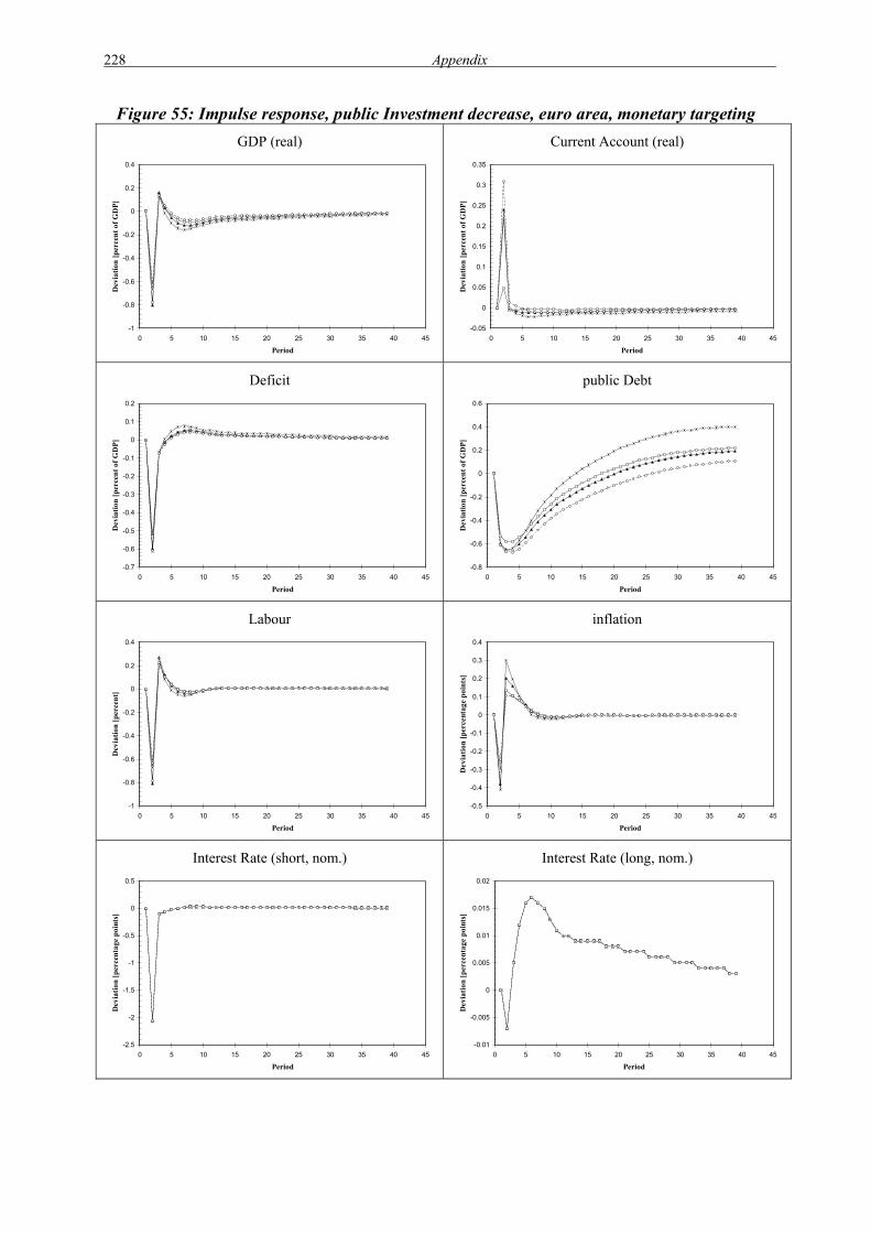
228 Appendix
Figure 55: Impulse response, public Investment decrease, euro area, monetary targeting GDP (real)
-1
-0.8
-0.6
-0.4
-0.2
0
0.2
0.4
0 5 10 15 20 25 30 35 40 45
Period
Dev
iatio
n [p
erce
nt o
f GD
P]
Current Account (real)
-0.05
0
0.05
0.1
0.15
0.2
0.25
0.3
0.35
0 5 10 15 20 25 30 35 40 45
Period
Dev
iatio
n [p
erce
nt o
f GD
P]
Deficit
-0.7
-0.6
-0.5
-0.4
-0.3
-0.2
-0.1
0
0.1
0.2
0 5 10 15 20 25 30 35 40 45
Period
Dev
iatio
n [p
erce
nt o
f GD
P]
public Debt
-0.8
-0.6
-0.4
-0.2
0
0.2
0.4
0.6
0 5 10 15 20 25 30 35 40 45
Period
Dev
iatio
n [p
erce
nt o
f GD
P]
Labour
-1
-0.8
-0.6
-0.4
-0.2
0
0.2
0.4
0 5 10 15 20 25 30 35 40 45
Period
Dev
iatio
n [p
erce
nt]
inflation
-0.5
-0.4
-0.3
-0.2
-0.1
0
0.1
0.2
0.3
0.4
0 5 10 15 20 25 30 35 40 45
Period
Dev
iatio
n [p
erce
ntag
e po
ints
]
Interest Rate (short, nom.)
-2.5
-2
-1.5
-1
-0.5
0
0.5
0 5 10 15 20 25 30 35 40 45
Period
Dev
iatio
n [p
erce
ntag
e po
ints
]
Interest Rate (long, nom.)
-0.01
-0.005
0
0.005
0.01
0.015
0.02
0 5 10 15 20 25 30 35 40 45
Period
Dev
iatio
n [p
erce
ntag
e po
ints
]

Appendix 229
Figure 56: Impulse response, public investment decrease, Germany, monetary targeting GDP (real)
-0.8
-0.6
-0.4
-0.2
0
0.2
0.4
0.6
0.8
0 5 10 15 20 25 30 35 40 45
Period
Dev
iatio
n [p
erce
nt o
f GD
P]
Current Account (real)
-0.1
-0.05
0
0.05
0.1
0.15
0.2
0.25
0 5 10 15 20 25 30 35 40 45
Period
Dev
iatio
n [p
erce
nt o
f GD
P]
Deficit
-0.7
-0.6
-0.5
-0.4
-0.3
-0.2
-0.1
0
0.1
0.2
0 5 10 15 20 25 30 35 40 45
Period
Dev
iatio
n [p
erce
nt o
f GD
P]
public Debt
-0.7
-0.6
-0.5
-0.4
-0.3
-0.2
-0.1
0
0.1
0.2
0 5 10 15 20 25 30 35 40 45
Period
Dev
iatio
n [p
erce
nt o
f GD
P]
Labour
-0.8
-0.6
-0.4
-0.2
0
0.2
0.4
0.6
0.8
0 5 10 15 20 25 30 35 40 45
Period
Dev
iatio
n [p
erce
nt]
inflation
-0.3
-0.2
-0.1
0
0.1
0.2
0.3
0.4
0.5
0 5 10 15 20 25 30 35 40 45
Period
Dev
iatio
n [p
erce
ntag
e po
ints
]
Interest Rate (short, nom.)
-2
-1.8
-1.6
-1.4
-1.2
-1
-0.8
-0.6
-0.4
-0.2
0
0.2
0 5 10 15 20 25 30 35 40 45
Period
Dev
iatio
n [p
erce
ntag
e po
ints
]
Interest Rate (long, nom.)
0
0.0005
0.001
0.0015
0.002
0.0025
0.003
0.0035
0.004
0.0045
0 5 10 15 20 25 30 35 40 45
Period
Dev
iatio
n [p
erce
ntag
e po
ints
]

230 Appendix
Figure 57: Impulse response, public investment decrease, Austria, monetary targeting GDP (real)
-1.2
-1
-0.8
-0.6
-0.4
-0.2
0
0.2
0.4
0 5 10 15 20 25 30 35 40 45
Period
Dev
iatio
n [p
erce
nt o
f GD
P]
Current Account (real)
-0.05
0
0.05
0.1
0.15
0.2
0.25
0.3
0.35
0.4
0 5 10 15 20 25 30 35 40 45
Period
Dev
iatio
n [p
erce
nt o
f GD
P]
Deficit
-0.4
-0.35
-0.3
-0.25
-0.2
-0.15
-0.1
-0.05
0
0.05
0 5 10 15 20 25 30 35 40 45
Period
Dev
iatio
n [p
erce
nt o
f GD
P]
public Debt
-0.5
-0.4
-0.3
-0.2
-0.1
0
0.1
0.2
0 5 10 15 20 25 30 35 40 45
Period
Dev
iatio
n [p
erce
nt o
f GD
P]
Labour
-1.2
-1
-0.8
-0.6
-0.4
-0.2
0
0.2
0.4
0 5 10 15 20 25 30 35 40 45
Period
Dev
iatio
n [p
erce
nt]
inflation
-0.6
-0.5
-0.4
-0.3
-0.2
-0.1
0
0.1
0.2
0.3
0 5 10 15 20 25 30 35 40 45
Period
Dev
iatio
n [p
erce
ntag
e po
ints
]
Interest Rate (short, nom.)
-0.025
-0.02
-0.015
-0.01
-0.005
0
0.005
0 5 10 15 20 25 30 35 40 45
Period
Dev
iatio
n [p
erce
ntag
e po
ints
]
Interest Rate (long, nom.)
-0.0015
-0.001
-0.0005
0
0.0005
0.001
0.0015
0 5 10 15 20 25 30 35 40 45
Period
Dev
iatio
n [p
erce
ntag
e po
ints
]

Appendix 231
Figure 58: Impulse response, public investment decrease, France, monetary targeting GDP (real)
-1.4
-1.2
-1
-0.8
-0.6
-0.4
-0.2
0
0.2
0.4
0 5 10 15 20 25 30 35 40 45
Period
Dev
iatio
n [p
erce
nt o
f GD
P]
Current Account (real)
-0.1
-0.05
0
0.05
0.1
0.15
0.2
0.25
0.3
0.35
0 5 10 15 20 25 30 35 40 45
Period
Dev
iatio
n [p
erce
nt o
f GD
P]
Deficit
-0.4
-0.35
-0.3
-0.25
-0.2
-0.15
-0.1
-0.05
0
0.05
0.1
0 5 10 15 20 25 30 35 40 45
Period
Dev
iatio
n [p
erce
nt o
f GD
P]
public Debt
-0.6
-0.5
-0.4
-0.3
-0.2
-0.1
0
0.1
0.2
0.3
0 5 10 15 20 25 30 35 40 45
Period
Dev
iatio
n [p
erce
nt o
f GD
P]
Labour
-1.6
-1.4
-1.2
-1
-0.8
-0.6
-0.4
-0.2
0
0.2
0.4
0.6
0 5 10 15 20 25 30 35 40 45
Period
Dev
iatio
n [p
erce
nt]
inflation
-0.8
-0.6
-0.4
-0.2
0
0.2
0.4
0.6
0 5 10 15 20 25 30 35 40 45
Period
Dev
iatio
n [p
erce
ntag
e po
ints
]
Interest Rate (short, nom.)
-0.1
-0.08
-0.06
-0.04
-0.02
0
0.02
0 5 10 15 20 25 30 35 40 45
Period
Dev
iatio
n [p
erce
ntag
e po
ints
]
Interest Rate (long, nom.)
-0.003
-0.002
-0.001
0
0.001
0.002
0.003
0.004
0.005
0 5 10 15 20 25 30 35 40 45
Period
Dev
iatio
n [p
erce
ntag
e po
ints
]

232 Appendix
Figure 59: Impulse response, public investment decrease, Italy, monetary targeting GDP (real)
-1.4
-1.2
-1
-0.8
-0.6
-0.4
-0.2
0
0.2
0.4
0 5 10 15 20 25 30 35 40 45
Period
Dev
iatio
n [p
erce
nt o
f GD
P]
Current Account (real)
-0.1
-0.05
0
0.05
0.1
0.15
0.2
0.25
0.3
0 5 10 15 20 25 30 35 40 45
Period
Dev
iatio
n [p
erce
nt o
f GD
P]
Deficit
-0.35
-0.3
-0.25
-0.2
-0.15
-0.1
-0.05
0
0.05
0.1
0 5 10 15 20 25 30 35 40 45
Period
Dev
iatio
n [p
erce
nt o
f GD
P]
public Debt
-0.5
-0.4
-0.3
-0.2
-0.1
0
0.1
0.2
0.3
0.4
0.5
0.6
0 5 10 15 20 25 30 35 40 45
Period
Dev
iatio
n [p
erce
nt o
f GD
P]
Labour
-1.4
-1.2
-1
-0.8
-0.6
-0.4
-0.2
0
0.2
0.4
0.6
0 5 10 15 20 25 30 35 40 45
Period
Dev
iatio
n [p
erce
nt]
inflation
-1
-0.8
-0.6
-0.4
-0.2
0
0.2
0.4
0.6
0 5 10 15 20 25 30 35 40 45
Period
Dev
iatio
n [p
erce
ntag
e po
ints
]
Interest Rate (short, nom.)
-0.07
-0.06
-0.05
-0.04
-0.03
-0.02
-0.01
0
0.01
0.02
0 5 10 15 20 25 30 35 40 45
Period
Dev
iatio
n [p
erce
ntag
e po
ints
]
Interest Rate (long, nom.)
-0.002
-0.001
0
0.001
0.002
0.003
0.004
0.005
0.006
0 5 10 15 20 25 30 35 40 45
Period
Dev
iatio
n [p
erce
ntag
e po
ints
]

Appendix 233
Figure 60: Impulse response, tax increase, euro area, inflation targeting GDP (real)
-0.3
-0.25
-0.2
-0.15
-0.1
-0.05
0
0.05
0.1
0.15
0.2
0 5 10 15 20 25 30 35 40 45
Period
Dev
iatio
n [p
erce
nt o
f GD
P]
Current Account (real)
0
0.05
0.1
0.15
0.2
0.25
0.3
0.35
0.4
0 5 10 15 20 25 30 35 40 45
Period
Dev
iatio
n [p
erce
nt o
f GD
P]
Deficit
-1
-0.9
-0.8
-0.7
-0.6
-0.5
-0.4
-0.3
-0.2
-0.1
0
0 5 10 15 20 25 30 35 40 45
Period
Dev
iatio
n [p
erce
nt o
f GD
P]
public Debt
-1.2
-1
-0.8
-0.6
-0.4
-0.2
0
0 5 10 15 20 25 30 35 40 45
Period
Dev
iatio
n [p
erce
nt o
f GD
P]
Labour
-0.3
-0.25
-0.2
-0.15
-0.1
-0.05
0
0.05
0.1
0.15
0.2
0 5 10 15 20 25 30 35 40 45
Period
Dev
iatio
n [p
erce
nt]
inflation
-0.06
-0.04
-0.02
0
0.02
0.04
0.06
0 5 10 15 20 25 30 35 40 45
Period
Dev
iatio
n [p
erce
ntag
e po
ints
]
Interest Rate (short, nom.)
-2.5
-2
-1.5
-1
-0.5
0
0 5 10 15 20 25 30 35 40 45
Period
Dev
iatio
n [p
erce
ntag
e po
ints
]
Interest Rate (long, nom.)
-0.035
-0.03
-0.025
-0.02
-0.015
-0.01
-0.005
0
0 5 10 15 20 25 30 35 40 45
Period
Dev
iatio
n [p
erce
ntag
e po
ints
]

234 Appendix
Figure 61: Impulse response, tax increase, Germany, inflation targeting GDP (real)
-0.6
-0.5
-0.4
-0.3
-0.2
-0.1
0
0.1
0.2
0 5 10 15 20 25 30 35 40 45
Period
Dev
iatio
n [p
erce
nt o
f GD
P]
Current Account (real)
-0.1
-0.05
0
0.05
0.1
0.15
0.2
0.25
0.3
0 5 10 15 20 25 30 35 40 45
Period
Dev
iatio
n [p
erce
nt o
f GD
P]
Deficit
-0.8
-0.7
-0.6
-0.5
-0.4
-0.3
-0.2
-0.1
0
0.1
0 5 10 15 20 25 30 35 40 45
Period
Dev
iatio
n [p
erce
nt o
f GD
P]
public Debt
-0.9
-0.8
-0.7
-0.6
-0.5
-0.4
-0.3
-0.2
-0.1
0
0 5 10 15 20 25 30 35 40 45
Period
Dev
iatio
n [p
erce
nt o
f GD
P]
Labour
-0.6
-0.5
-0.4
-0.3
-0.2
-0.1
0
0.1
0.2
0 5 10 15 20 25 30 35 40 45
Period
Dev
iatio
n [p
erce
nt]
inflation
-0.25
-0.2
-0.15
-0.1
-0.05
0
0.05
0.1
0.15
0 5 10 15 20 25 30 35 40 45
Period
Dev
iatio
n [p
erce
ntag
e po
ints
]
Interest Rate (short, nom.)
-0.7
-0.6
-0.5
-0.4
-0.3
-0.2
-0.1
0
0 5 10 15 20 25 30 35 40 45
Period
Dev
iatio
n [p
erce
ntag
e po
ints
]
Interest Rate (long, nom.)
-0.012
-0.01
-0.008
-0.006
-0.004
-0.002
0
0 5 10 15 20 25 30 35 40 45
Period
Dev
iatio
n [p
erce
ntag
e po
ints
]

Appendix 235
Figure 62: Impulse response, tax increase, Austria, inflation targeting GDP (real)
-0.6
-0.5
-0.4
-0.3
-0.2
-0.1
0
0.1
0.2
0 5 10 15 20 25 30 35 40 45
Period
Dev
iatio
n [p
erce
nt o
f GD
P]
Current Account (real)
-0.05
0
0.05
0.1
0.15
0.2
0.25
0.3
0.35
0.4
0.45
0 5 10 15 20 25 30 35 40 45
Period
Dev
iatio
n [p
erce
nt o
f GD
P]
Deficit
-0.8
-0.7
-0.6
-0.5
-0.4
-0.3
-0.2
-0.1
0
0.1
0 5 10 15 20 25 30 35 40 45
Period
Dev
iatio
n [p
erce
nt o
f GD
P]
public Debt
-0.8
-0.7
-0.6
-0.5
-0.4
-0.3
-0.2
-0.1
0
0.1
0 5 10 15 20 25 30 35 40 45
Period
Dev
iatio
n [p
erce
nt o
f GD
P]
Labour
-0.6
-0.5
-0.4
-0.3
-0.2
-0.1
0
0.1
0.2
0 5 10 15 20 25 30 35 40 45
Period
Dev
iatio
n [p
erce
nt]
inflation
-0.25
-0.2
-0.15
-0.1
-0.05
0
0.05
0.1
0 5 10 15 20 25 30 35 40 45
Period
Dev
iatio
n [p
erce
ntag
e po
ints
]
Interest Rate (short, nom.)
-0.06
-0.05
-0.04
-0.03
-0.02
-0.01
0
0 5 10 15 20 25 30 35 40 45
Period
Dev
iatio
n [p
erce
ntag
e po
ints
]
Interest Rate (long, nom.)
-0.0012
-0.001
-0.0008
-0.0006
-0.0004
-0.0002
0
0 5 10 15 20 25 30 35 40 45
Period
Dev
iatio
n [p
erce
ntag
e po
ints
]

236 Appendix
Figure 63: Impulse response, tax increase, France, inflation targeting GDP (real)
-0.7
-0.6
-0.5
-0.4
-0.3
-0.2
-0.1
0
0.1
0.2
0.3
0 5 10 15 20 25 30 35 40 45
Period
Dev
iatio
n [p
erce
nt o
f GD
P]
Current Account (real)
-0.1
-0.05
0
0.05
0.1
0.15
0.2
0.25
0.3
0.35
0 5 10 15 20 25 30 35 40 45
Period
Dev
iatio
n [p
erce
nt o
f GD
P]
Deficit
-0.8
-0.7
-0.6
-0.5
-0.4
-0.3
-0.2
-0.1
0
0.1
0 5 10 15 20 25 30 35 40 45
Period
Dev
iatio
n [p
erce
nt o
f GD
P]
public Debt
-0.9
-0.8
-0.7
-0.6
-0.5
-0.4
-0.3
-0.2
-0.1
0
0 5 10 15 20 25 30 35 40 45
Period
Dev
iatio
n [p
erce
nt o
f GD
P]
Labour
-0.7
-0.6
-0.5
-0.4
-0.3
-0.2
-0.1
0
0.1
0.2
0.3
0 5 10 15 20 25 30 35 40 45
Period
Dev
iatio
n [p
erce
nt]
inflation
-0.3
-0.25
-0.2
-0.15
-0.1
-0.05
0
0.05
0.1
0.15
0 5 10 15 20 25 30 35 40 45
Period
Dev
iatio
n [p
erce
ntag
e po
ints
]
Interest Rate (short, nom.)
-0.6
-0.5
-0.4
-0.3
-0.2
-0.1
0
0 5 10 15 20 25 30 35 40 45
Period
Dev
iatio
n [p
erce
ntag
e po
ints
]
Interest Rate (long, nom.)
-0.008
-0.007
-0.006
-0.005
-0.004
-0.003
-0.002
-0.001
0
0 5 10 15 20 25 30 35 40 45
Period
Dev
iatio
n [p
erce
ntag
e po
ints
]

Appendix 237
Figure 64: Impulse response, tax increase, Italy, inflation targeting GDP (real)
-0.7
-0.6
-0.5
-0.4
-0.3
-0.2
-0.1
0
0.1
0.2
0.3
0 5 10 15 20 25 30 35 40 45
Period
Dev
iatio
n [p
erce
nt o
f GD
P]
Current Account (real)
-0.1
-0.05
0
0.05
0.1
0.15
0.2
0.25
0.3
0 5 10 15 20 25 30 35 40 45
Period
Dev
iatio
n [p
erce
nt o
f GD
P]
Deficit
-0.7
-0.6
-0.5
-0.4
-0.3
-0.2
-0.1
0
0.1
0 5 10 15 20 25 30 35 40 45
Period
Dev
iatio
n [p
erce
nt o
f GD
P]
public Debt
-0.8
-0.7
-0.6
-0.5
-0.4
-0.3
-0.2
-0.1
0
0 5 10 15 20 25 30 35 40 45
Period
Dev
iatio
n [p
erce
nt o
f GD
P]
Labour
-0.7
-0.6
-0.5
-0.4
-0.3
-0.2
-0.1
0
0.1
0.2
0.3
0 5 10 15 20 25 30 35 40 45
Period
Dev
iatio
n [p
erce
nt]
inflation
-0.4
-0.3
-0.2
-0.1
0
0.1
0.2
0 5 10 15 20 25 30 35 40 45
Period
Dev
iatio
n [p
erce
ntag
e po
ints
]
Interest Rate (short, nom.)
-0.5
-0.45
-0.4
-0.35
-0.3
-0.25
-0.2
-0.15
-0.1
-0.05
0
0 5 10 15 20 25 30 35 40 45
Period
Dev
iatio
n [p
erce
ntag
e po
ints
]
Interest Rate (long, nom.)
-0.0045
-0.004
-0.0035
-0.003
-0.0025
-0.002
-0.0015
-0.001
-0.0005
0
0 5 10 15 20 25 30 35 40 45
Period
Dev
iatio
n [p
erce
ntag
e po
ints
]

238 Appendix
Figure 65: Impulse response, public consumption decrease, euro area, inflation targeting GDP (real)
-0.5
-0.4
-0.3
-0.2
-0.1
0
0.1
0.2
0.3
0 5 10 15 20 25 30 35 40 45
Period
Dev
iatio
n [p
erce
nt o
f GD
P]
Current Account (real)
0
0.1
0.2
0.3
0.4
0.5
0.6
0 5 10 15 20 25 30 35 40 45
Period
Dev
iatio
n [p
erce
nt o
f GD
P]
Deficit
-1
-0.9
-0.8
-0.7
-0.6
-0.5
-0.4
-0.3
-0.2
-0.1
0
0 5 10 15 20 25 30 35 40 45
Period
Dev
iatio
n [p
erce
nt o
f GD
P]
public Debt
-1.2
-1
-0.8
-0.6
-0.4
-0.2
0
0 5 10 15 20 25 30 35 40 45
Period
Dev
iatio
n [p
erce
nt o
f GD
P]
Labour
-0.5
-0.4
-0.3
-0.2
-0.1
0
0.1
0.2
0.3
0 5 10 15 20 25 30 35 40 45
Period
Dev
iatio
n [p
erce
nt]
inflation
-0.1
-0.08
-0.06
-0.04
-0.02
0
0.02
0.04
0.06
0.08
0 5 10 15 20 25 30 35 40 45
Period
Dev
iatio
n [p
erce
ntag
e po
ints
]
Interest Rate (short, nom.)
-3
-2.5
-2
-1.5
-1
-0.5
0
0 5 10 15 20 25 30 35 40 45
Period
Dev
iatio
n [p
erce
ntag
e po
ints
]
Interest Rate (long, nom.)
-0.05
-0.045
-0.04
-0.035
-0.03
-0.025
-0.02
-0.015
-0.01
-0.005
0
0 5 10 15 20 25 30 35 40 45
Period
Dev
iatio
n [p
erce
ntag
e po
ints
]

Appendix 239
Figure 66: Impulse response, public consumption decrease, Germany, inflation targeting GDP (real)
-0.8
-0.6
-0.4
-0.2
0
0.2
0.4
0 5 10 15 20 25 30 35 40 45
Period
Dev
iatio
n [p
erce
nt o
f GD
P]
Current Account (real)
-0.15
-0.1
-0.05
0
0.05
0.1
0.15
0.2
0.25
0.3
0.35
0.4
0 5 10 15 20 25 30 35 40 45
Period
Dev
iatio
n [p
erce
nt o
f GD
P]
Deficit
-0.7
-0.6
-0.5
-0.4
-0.3
-0.2
-0.1
0
0.1
0 5 10 15 20 25 30 35 40 45
Period
Dev
iatio
n [p
erce
nt o
f GD
P]
public Debt
-0.8
-0.7
-0.6
-0.5
-0.4
-0.3
-0.2
-0.1
0
0 5 10 15 20 25 30 35 40 45
Period
Dev
iatio
n [p
erce
nt o
f GD
P]
Labour
-0.8
-0.6
-0.4
-0.2
0
0.2
0.4
0 5 10 15 20 25 30 35 40 45
Period
Dev
iatio
n [p
erce
nt]
inflation
-0.3
-0.25
-0.2
-0.15
-0.1
-0.05
0
0.05
0.1
0.15
0.2
0 5 10 15 20 25 30 35 40 45
Period
Dev
iatio
n [p
erce
ntag
e po
ints
]
Interest Rate (short, nom.)
-0.9
-0.8
-0.7
-0.6
-0.5
-0.4
-0.3
-0.2
-0.1
0
0 5 10 15 20 25 30 35 40 45
Period
Dev
iatio
n [p
erce
ntag
e po
ints
]
Interest Rate (long, nom.)
-0.016
-0.014
-0.012
-0.01
-0.008
-0.006
-0.004
-0.002
0
0 5 10 15 20 25 30 35 40 45
Period
Dev
iatio
n [p
erce
ntag
e po
ints
]

240 Appendix
Figure 67: Impulse response, public consumption decrease, Austria, inflation targeting GDP (real)
-0.8
-0.6
-0.4
-0.2
0
0.2
0.4
0 5 10 15 20 25 30 35 40 45
Period
Dev
iatio
n [p
erce
nt o
f GD
P]
Current Account (real)
-0.1
0
0.1
0.2
0.3
0.4
0.5
0.6
0 5 10 15 20 25 30 35 40 45
Period
Dev
iatio
n [p
erce
nt o
f GD
P]
Deficit
-0.6
-0.5
-0.4
-0.3
-0.2
-0.1
0
0.1
0 5 10 15 20 25 30 35 40 45
Period
Dev
iatio
n [p
erce
nt o
f GD
P]
public Debt
-0.8
-0.7
-0.6
-0.5
-0.4
-0.3
-0.2
-0.1
0
0.1
0 5 10 15 20 25 30 35 40 45
Period
Dev
iatio
n [p
erce
nt o
f GD
P]
Labour
-0.8
-0.6
-0.4
-0.2
0
0.2
0.4
0 5 10 15 20 25 30 35 40 45
Period
Dev
iatio
n [p
erce
nt]
inflation
-0.35
-0.3
-0.25
-0.2
-0.15
-0.1
-0.05
0
0.05
0.1
0.15
0 5 10 15 20 25 30 35 40 45
Period
Dev
iatio
n [p
erce
ntag
e po
ints
]
Interest Rate (short, nom.)
-0.09
-0.08
-0.07
-0.06
-0.05
-0.04
-0.03
-0.02
-0.01
0
0 5 10 15 20 25 30 35 40 45
Period
Dev
iatio
n [p
erce
ntag
e po
ints
]
Interest Rate (long, nom.)
-0.0025
-0.002
-0.0015
-0.001
-0.0005
0
0 5 10 15 20 25 30 35 40 45
Period
Dev
iatio
n [p
erce
ntag
e po
ints
]
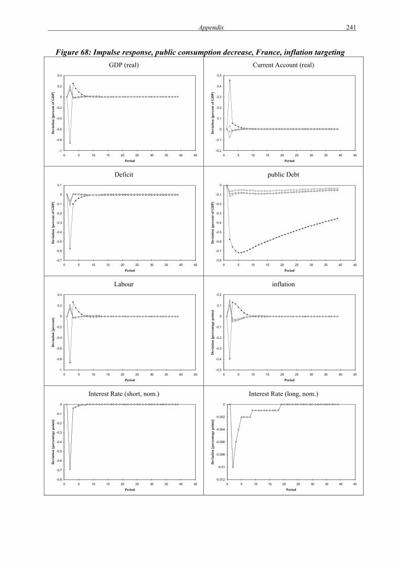
Appendix 241
Figure 68: Impulse response, public consumption decrease, France, inflation targeting GDP (real)
-1
-0.8
-0.6
-0.4
-0.2
0
0.2
0.4
0 5 10 15 20 25 30 35 40 45
Period
Dev
iatio
n [p
erce
nt o
f GD
P]
Current Account (real)
-0.2
-0.1
0
0.1
0.2
0.3
0.4
0.5
0 5 10 15 20 25 30 35 40 45
Period
Dev
iatio
n [p
erce
nt o
f GD
P]
Deficit
-0.7
-0.6
-0.5
-0.4
-0.3
-0.2
-0.1
0
0.1
0 5 10 15 20 25 30 35 40 45
Period
Dev
iatio
n [p
erce
nt o
f GD
P]
public Debt
-0.8
-0.7
-0.6
-0.5
-0.4
-0.3
-0.2
-0.1
0
0 5 10 15 20 25 30 35 40 45
Period
Dev
iatio
n [p
erce
nt o
f GD
P]
Labour
-1
-0.8
-0.6
-0.4
-0.2
0
0.2
0.4
0 5 10 15 20 25 30 35 40 45
Period
Dev
iatio
n [p
erce
nt]
inflation
-0.5
-0.4
-0.3
-0.2
-0.1
0
0.1
0.2
0 5 10 15 20 25 30 35 40 45
Period
Dev
iatio
n [p
erce
ntag
e po
ints
]
Interest Rate (short, nom.)
-0.8
-0.7
-0.6
-0.5
-0.4
-0.3
-0.2
-0.1
0
0 5 10 15 20 25 30 35 40 45
Period
Dev
iatio
n [p
erce
ntag
e po
ints
]
Interest Rate (long, nom.)
-0.012
-0.01
-0.008
-0.006
-0.004
-0.002
0
0 5 10 15 20 25 30 35 40 45
Period
Dev
iatio
n [p
erce
ntag
e po
ints
]

242 Appendix
Figure 69: Impulse response, public consumption decrease, Italy, inflation targeting GDP (real)
-1
-0.8
-0.6
-0.4
-0.2
0
0.2
0.4
0 5 10 15 20 25 30 35 40 45
Period
Dev
iatio
n [p
erce
nt o
f GD
P]
Current Account (real)
-0.1
-0.05
0
0.05
0.1
0.15
0.2
0.25
0.3
0.35
0.4
0.45
0 5 10 15 20 25 30 35 40 45
Period
Dev
iatio
n [p
erce
nt o
f GD
P]
Deficit
-0.6
-0.5
-0.4
-0.3
-0.2
-0.1
0
0.1
0 5 10 15 20 25 30 35 40 45
Period
Dev
iatio
n [p
erce
nt o
f GD
P]
public Debt
-0.8
-0.7
-0.6
-0.5
-0.4
-0.3
-0.2
-0.1
0
0 5 10 15 20 25 30 35 40 45
Period
Dev
iatio
n [p
erce
nt o
f GD
P]
Labour
-1
-0.8
-0.6
-0.4
-0.2
0
0.2
0.4
0 5 10 15 20 25 30 35 40 45
Period
Dev
iatio
n [p
erce
nt]
inflation
-0.6
-0.5
-0.4
-0.3
-0.2
-0.1
0
0.1
0.2
0.3
0 5 10 15 20 25 30 35 40 45
Period
Dev
iatio
n [p
erce
ntag
e po
ints
]
Interest Rate (short, nom.)
-0.8
-0.7
-0.6
-0.5
-0.4
-0.3
-0.2
-0.1
0
0 5 10 15 20 25 30 35 40 45
Period
Dev
iatio
n [p
erce
ntag
e po
ints
]
Interest Rate (long, nom.)
-0.007
-0.006
-0.005
-0.004
-0.003
-0.002
-0.001
0
0 5 10 15 20 25 30 35 40 45
Period
Dev
iatio
n [p
erce
ntag
e po
ints
]

Appendix 243
Figure 70: Impulse response, public investment decrease, euro area, inflation targeting GDP (real)
-0.45
-0.4
-0.35
-0.3
-0.25
-0.2
-0.15
-0.1
-0.05
0
0.05
0 5 10 15 20 25 30 35 40 45
Period
Dev
iatio
n [p
erce
nt o
f GD
P]
Current Account (real)
-0.05
0
0.05
0.1
0.15
0.2
0.25
0.3
0.35
0.4
0.45
0 5 10 15 20 25 30 35 40 45
Period
Dev
iatio
n [p
erce
nt o
f GD
P]
Deficit
-0.9
-0.8
-0.7
-0.6
-0.5
-0.4
-0.3
-0.2
-0.1
0
0.1
0 5 10 15 20 25 30 35 40 45
Period
Dev
iatio
n [p
erce
nt o
f GD
P]
public Debt
-1
-0.8
-0.6
-0.4
-0.2
0
0.2
0.4
0 5 10 15 20 25 30 35 40 45
Period
Dev
iatio
n [p
erce
nt o
f GD
P]
Labour
-0.5
-0.4
-0.3
-0.2
-0.1
0
0.1
0.2
0 5 10 15 20 25 30 35 40 45
Period
Dev
iatio
n [p
erce
nt]
inflation
-0.08
-0.06
-0.04
-0.02
0
0.02
0.04
0.06
0.08
0.1
0.12
0 5 10 15 20 25 30 35 40 45
Period
Dev
iatio
n [p
erce
ntag
e po
ints
]
Interest Rate (short, nom.)
-4
-3.5
-3
-2.5
-2
-1.5
-1
-0.5
0
0.5
0 5 10 15 20 25 30 35 40 45
Period
Dev
iatio
n [p
erce
ntag
e po
ints
]
Interest Rate (long, nom.)
0
0.002
0.004
0.006
0.008
0.01
0.012
0.014
0 5 10 15 20 25 30 35 40 45
Period
Dev
iatio
n [p
erce
ntag
e po
ints
]

244 Appendix
Figure 71: Impulse response, public investment decrease, Germany, inflation targeting GDP (real)
-1
-0.8
-0.6
-0.4
-0.2
0
0.2
0.4
0 5 10 15 20 25 30 35 40 45
Period
Dev
iatio
n [p
erce
nt o
f GD
P]
Current Account (real)
-0.05
0
0.05
0.1
0.15
0.2
0.25
0 5 10 15 20 25 30 35 40 45
Period
Dev
iatio
n [p
erce
nt o
f GD
P]
Deficit
-0.5
-0.4
-0.3
-0.2
-0.1
0
0.1
0 5 10 15 20 25 30 35 40 45
Period
Dev
iatio
n [p
erce
nt o
f GD
P]
public Debt
-0.6
-0.5
-0.4
-0.3
-0.2
-0.1
0
0.1
0.2
0.3
0 5 10 15 20 25 30 35 40 45
Period
Dev
iatio
n [p
erce
nt o
f GD
P]
Labour
-1
-0.8
-0.6
-0.4
-0.2
0
0.2
0.4
0 5 10 15 20 25 30 35 40 45
Period
Dev
iatio
n [p
erce
nt]
inflation
-0.4
-0.3
-0.2
-0.1
0
0.1
0.2
0.3
0 5 10 15 20 25 30 35 40 45
Period
Dev
iatio
n [p
erce
ntag
e po
ints
]
Interest Rate (short, nom.)
-1.2
-1
-0.8
-0.6
-0.4
-0.2
0
0.2
0 5 10 15 20 25 30 35 40 45
Period
Dev
iatio
n [p
erce
ntag
e po
ints
]
Interest Rate (long, nom.)
0
0.0005
0.001
0.0015
0.002
0.0025
0.003
0.0035
0 5 10 15 20 25 30 35 40 45
Period
Dev
iatio
n [p
erce
ntag
e po
ints
]
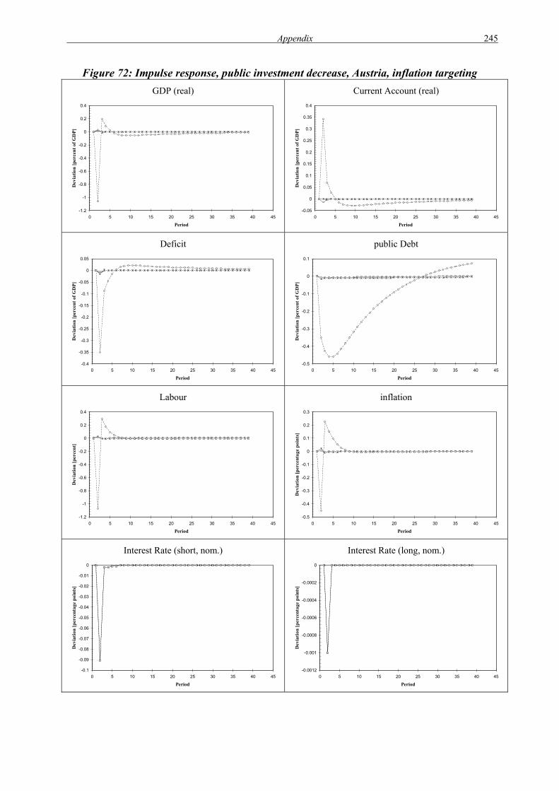
Appendix 245
Figure 72: Impulse response, public investment decrease, Austria, inflation targeting GDP (real)
-1.2
-1
-0.8
-0.6
-0.4
-0.2
0
0.2
0.4
0 5 10 15 20 25 30 35 40 45
Period
Dev
iatio
n [p
erce
nt o
f GD
P]
Current Account (real)
-0.05
0
0.05
0.1
0.15
0.2
0.25
0.3
0.35
0.4
0 5 10 15 20 25 30 35 40 45
Period
Dev
iatio
n [p
erce
nt o
f GD
P]
Deficit
-0.4
-0.35
-0.3
-0.25
-0.2
-0.15
-0.1
-0.05
0
0.05
0 5 10 15 20 25 30 35 40 45
Period
Dev
iatio
n [p
erce
nt o
f GD
P]
public Debt
-0.5
-0.4
-0.3
-0.2
-0.1
0
0.1
0 5 10 15 20 25 30 35 40 45
Period
Dev
iatio
n [p
erce
nt o
f GD
P]
Labour
-1.2
-1
-0.8
-0.6
-0.4
-0.2
0
0.2
0.4
0 5 10 15 20 25 30 35 40 45
Period
Dev
iatio
n [p
erce
nt]
inflation
-0.5
-0.4
-0.3
-0.2
-0.1
0
0.1
0.2
0.3
0 5 10 15 20 25 30 35 40 45
Period
Dev
iatio
n [p
erce
ntag
e po
ints
]
Interest Rate (short, nom.)
-0.1
-0.09
-0.08
-0.07
-0.06
-0.05
-0.04
-0.03
-0.02
-0.01
0
0 5 10 15 20 25 30 35 40 45
Period
Dev
iatio
n [p
erce
ntag
e po
ints
]
Interest Rate (long, nom.)
-0.0012
-0.001
-0.0008
-0.0006
-0.0004
-0.0002
0
0 5 10 15 20 25 30 35 40 45
Period
Dev
iatio
n [p
erce
ntag
e po
ints
]
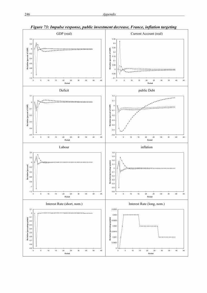
246 Appendix
Figure 73: Impulse response, public investment decrease, France, inflation targeting GDP (real)
-1.2
-1
-0.8
-0.6
-0.4
-0.2
0
0.2
0.4
0 5 10 15 20 25 30 35 40 45
Period
Dev
iatio
n [p
erce
nt o
f GD
P]
Current Account (real)
-0.1
-0.05
0
0.05
0.1
0.15
0.2
0.25
0.3
0.35
0 5 10 15 20 25 30 35 40 45
Period
Dev
iatio
n [p
erce
nt o
f GD
P]
Deficit
-0.5
-0.4
-0.3
-0.2
-0.1
0
0.1
0 5 10 15 20 25 30 35 40 45
Period
Dev
iatio
n [p
erce
nt o
f GD
P]
public Debt
-0.6
-0.5
-0.4
-0.3
-0.2
-0.1
0
0.1
0.2
0 5 10 15 20 25 30 35 40 45
Period
Dev
iatio
n [p
erce
nt o
f GD
P]
Labour
-1.2
-1
-0.8
-0.6
-0.4
-0.2
0
0.2
0.4
0 5 10 15 20 25 30 35 40 45
Period
Dev
iatio
n [p
erce
nt]
inflation
-0.6
-0.5
-0.4
-0.3
-0.2
-0.1
0
0.1
0.2
0.3
0.4
0 5 10 15 20 25 30 35 40 45
Period
Dev
iatio
n [p
erce
ntag
e po
ints
]
Interest Rate (short, nom.)
-0.9
-0.8
-0.7
-0.6
-0.5
-0.4
-0.3
-0.2
-0.1
0
0.1
0 5 10 15 20 25 30 35 40 45
Period
Dev
iatio
n [p
erce
ntag
e po
ints
]
Interest Rate (long, nom.)
0
0.0005
0.001
0.0015
0.002
0.0025
0.003
0.0035
0 5 10 15 20 25 30 35 40 45
Period
Dev
iatio
n [p
erce
ntag
e po
ints
]

Appendix 247
Figure 74: Impulse response, public investment decrease, Italy, inflation targeting GDP (real)
-1.2
-1
-0.8
-0.6
-0.4
-0.2
0
0.2
0.4
0 5 10 15 20 25 30 35 40 45
Period
Dev
iatio
n [p
erce
nt o
f GD
P]
Current Account (real)
-0.1
-0.05
0
0.05
0.1
0.15
0.2
0.25
0.3
0 5 10 15 20 25 30 35 40 45
Period
Dev
iatio
n [p
erce
nt o
f GD
P]
Deficit
-0.5
-0.4
-0.3
-0.2
-0.1
0
0.1
0 5 10 15 20 25 30 35 40 45
Period
Dev
iatio
n [p
erce
nt o
f GD
P]
public Debt
-0.6
-0.5
-0.4
-0.3
-0.2
-0.1
0
0.1
0.2
0.3
0.4
0.5
0 5 10 15 20 25 30 35 40 45
Period
Dev
iatio
n [p
erce
nt o
f GD
P]
Labour
-1.2
-1
-0.8
-0.6
-0.4
-0.2
0
0.2
0.4
0 5 10 15 20 25 30 35 40 45
Period
Dev
iatio
n [p
erce
nt]
inflation
-0.8
-0.6
-0.4
-0.2
0
0.2
0.4
0.6
0 5 10 15 20 25 30 35 40 45
Period
Dev
iatio
n [p
erce
ntag
e po
ints
]
Interest Rate (short, nom.)
-0.9
-0.8
-0.7
-0.6
-0.5
-0.4
-0.3
-0.2
-0.1
0
0.1
0 5 10 15 20 25 30 35 40 45
Period
Dev
iatio
n [p
erce
ntag
e po
ints
]
Interest Rate (long, nom.)
0
0.001
0.002
0.003
0.004
0.005
0.006
0.007
0.008
0 5 10 15 20 25 30 35 40 45
Period
Dev
iatio
n [p
erce
ntag
e po
ints
]

248 Appendix
The results can be summarised as follows: In each case, real GDP of the country/region
affected by the increase of lump-sum taxes (decrease of lump-sum transfers), decrease of
public consumption, or decrease of public investment falls in the year of the policy change,
overshoots then and returns to baseline values after about 5 years. Real current account
improves in the short run (both due to reduced import demand and improvement of terms of
trade). The government sector deficit falls in the first year and stays below baseline values for
5 more years. Government debt stays below baseline for a longer period. Employment
behaves qualitatively and quantitatively in a similar way as real GDP. The short-term interest
rate falls considerably, but only during the year of the policy shock. The long-term interest
rate falls much less but stays below baseline for more years.
The following differences between the effects of different policy instruments are found:
Short-run negative effects on GDP and employment are strongest under a decrease of public
investment, less so under a decrease of public consumption, and weakest under an increase of
lump-sum taxes or decrease of lump-sum transfers. As the public-sector deficit reacts
endogenously on GDP changes, the opposite is true for the deficit and the public debt.
Negative effects on short-term interest rates are strongest for the public investment decrease
and weakest for the tax increase/transfer decrease. For long-term interest rates and public
debt, there is an important difference: Upon a one-time tax increase/transfer decrease or
increase of public consumption, public debt returns monotonically and very slowly to the
baseline. After a decrease of public investment, however, long-term interest rates overshoot
and stay above baseline values, with negative effects on capital and wealth. This leads to
public debt overshooting in later periods of the simulation; hence the original improvement of
the public sector’s debtor position is reversed in the long run for the countries/regions affected
by the shock to public investment. From this, we can conclude that both the short-run and the
long-run effects clearly speak against using public investment as a means of consolidating the
budget of the public sector. The policy conclusion regarding the decision between the
instruments public consumption and taxes/transfers is not so clear, in particular if we keep in
mind that we have changed lump-sum taxes or transfers and hence neglected allocative effects
(in particular, higher distortions when raising income or consumption taxes); also distributive
effects are not considered in this macroeconomic analysis.
Differences between scenarios with different countries being shocked are largely as expected:
The own-country effects are comparable to the euro area shocks in terms of own GDP-ratios

Appendix 249
and percentage point values. Short-run negative GDP and employment effects are stronger
and hence deficit and debt effects are weaker for the smaller economies of Austria, Italy and
France than for Germany or especially the whole euro area. The latter result may be regarded
as an argument in favour of policy coordination across the euro area. Spillover effects to
countries not directly affected by the shock are positively related to the size of the country
directly affected: For the shock to Germany, they are relatively strong for GDP and
employment (and mostly anti-symmetric) but less so (and symmetric) for public deficit and
debt; for the shock to Austria, they are virtually non-existent. The (one-time) effect on the
common euro area short-term interest rate is non-negligible even in cases where only one
country is affected by the shock. For instance, in the case of tax increase/transfer decrease
with monetary targeting, the short-term interest rate falls by 1.3 percentage points under the
euro area shock, by 1 percentage point under the Germany shock, by 0.1 percentage points
under the France shock, by 0.08 percentage points under the Italy shock and by 0.03 under the
Austrian shock. This shows that there are considerable spillover effects on the common
financial sector within the euro area according to the MSG3 Model, even though spillover
effects on flow variables of the “real” sector of the economy (GDP and its components,
employment, etc.) are much smaller; effects on stocks (capital stock, private wealth) are again
stronger.
If we compare the impulse responses under the assumption of monetary targeting and of
inflation targeting by the ECB, respectively, the qualitative differences described above hold
under both monetary policy regimes. The main difference is in the short run: Under monetary
targeting (which in the MSG3 Model is equivalent to keeping money supply at fixed baseline
values), inflation moves parallel to GDP and employment in the country affected directly by
the shock (with changes amounting to roughly one half percentage point values than for these
variables). This means that in the first year, where the effects are strongest, inflation is lower
than in the baseline solution of the model. In later years, it can be higher, but never more than
by 0.6 percentage points (mostly much less). Under inflation targeting, the ECB reacts upon
the fall of inflation by increasing money supply, which keeps euro area average inflation
(though not necessarily inflation in all euro area countries) very close to zero. This
expansionary monetary policy weakens the decline of GDP and reinforces the decline of the
public deficit and (mainly in the case of the common euro area shock) of the short-term
interest rate. Although these short-run effects of inflation targeting are favourable, we do not
consider such a reaction of the ECB to be likely. Given the ECB’s primary objective of price

250 Appendix
stability, it is more plausible that the ECB will not react upon a one-time fall of GDP and
inflation by about one percent or less in an expansionary way, especially when the shock is
accompanied by a considerable (endogenous) fall of the short-term interest rate. Therefore,
we retain the assumption of monetary targeting for the ECB also in the simulations of
structural and budgetary policies in chapter 7, which imply qualitatively similar scenarios as
described above.

Appendix 251
Appendix 5: Spillover effects of combined structural and budgetary consolidation policies
In this Appendix, we present simulation results that show all possible combinations of the
effects of structural policies as assumed in section 7.1 and of budgetary consolidation policies
as assumed in section 7.2 of chapter 7. This serves to demonstrate how these two types of
policies interact and which kind of spillover effects exist between these policies, especially if
different countries (Germany and Italy, in our case) or the entire euro area implement one or
both of these policies. A summary interpretation of the results is given in section 7.3.

252 Appendix
Figure 75: Public consumption decrease and structural policy in Germany GDP (real)
-0,5
0
0,5
1
1,5
2
0 5 10 15 20 25 30 35 40 45
Period
Dev
iatio
n [p
erce
nt o
f GD
P]
Current Account (real)
-1
-0,5
0
0,5
1
1,5
2
0 5 10 15 20 25 30 35 40 45
Period
Dev
iatio
n [p
erce
nt o
f GD
P]
Deficit
-2,5
-2
-1,5
-1
-0,5
0
0,5
0 5 10 15 20 25 30 35 40 45
Period
Dev
iatio
n [p
erce
nt o
f GD
P]
Public Debt
-20
-18
-16
-14
-12
-10
-8
-6
-4
-2
0
0 5 10 15 20 25 30 35 40 45
Period
Dev
iatio
n [p
erce
nt o
f GD
P]
Labour
-0,8
-0,6
-0,4
-0,2
0
0,2
0,4
0,6
0,8
1
1,2
0 5 10 15 20 25 30 35 40 45
Period
Dev
iatio
n [p
erce
nt o
f GD
P]
Inflation
-1,5
-1
-0,5
0
0,5
1
1,5
0 5 10 15 20 25 30 35 40 45
Period
Dev
iatio
n [p
erce
ntag
e po
ints
]
Interest Rate (short, nom.)
-1,5
-1
-0,5
0
0,5
1
0 5 10 15 20 25 30 35 40 45
Period
Dev
iatio
n [p
erce
ntag
e po
ints
]
Interest Rate (long, nom.)
-0,7
-0,6
-0,5
-0,4
-0,3
-0,2
-0,1
0
0 5 10 15 20 25 30 35 40 45
Period
Dev
iatio
n [p
erce
ntag
e po
ints
]
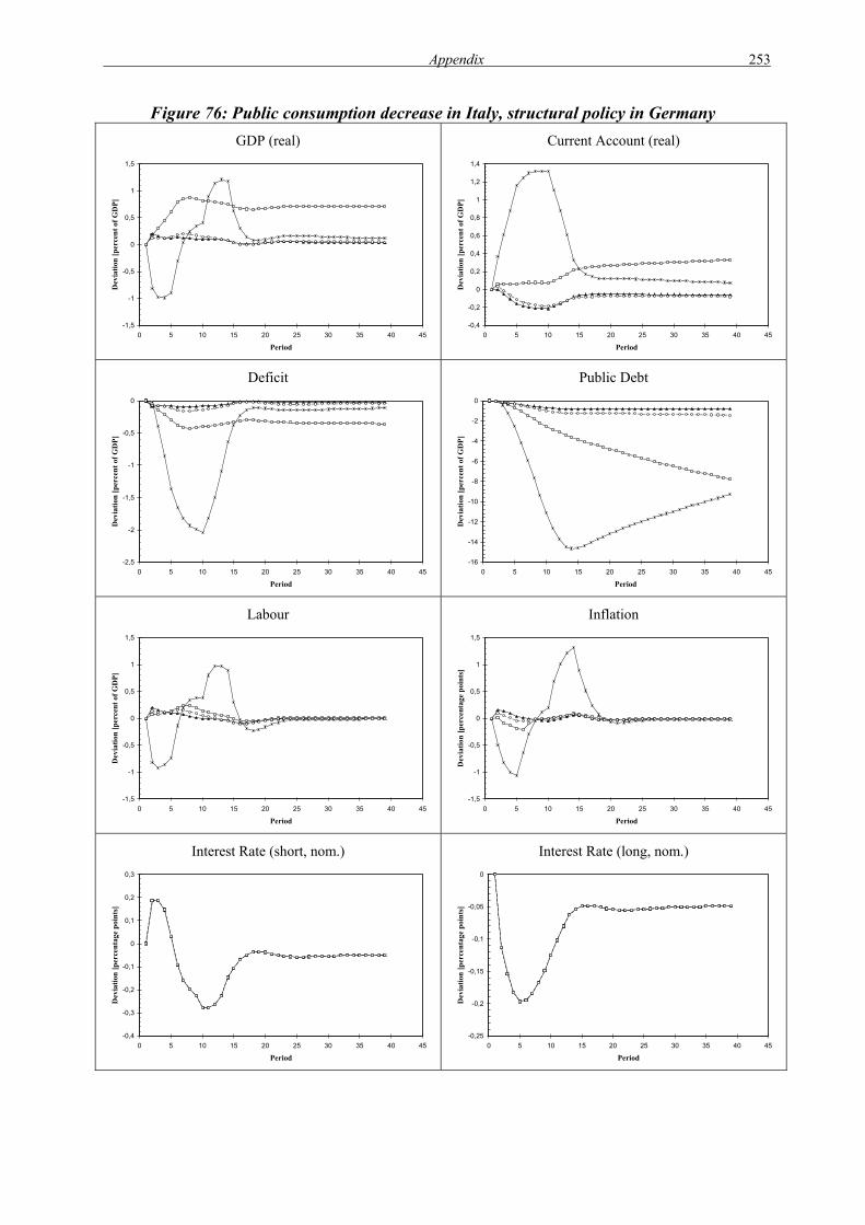
Appendix 253
Figure 76: Public consumption decrease in Italy, structural policy in Germany GDP (real)
-1,5
-1
-0,5
0
0,5
1
1,5
0 5 10 15 20 25 30 35 40 45
Period
Dev
iatio
n [p
erce
nt o
f GD
P]
Current Account (real)
-0,4
-0,2
0
0,2
0,4
0,6
0,8
1
1,2
1,4
0 5 10 15 20 25 30 35 40 45
Period
Dev
iatio
n [p
erce
nt o
f GD
P]
Deficit
-2,5
-2
-1,5
-1
-0,5
0
0 5 10 15 20 25 30 35 40 45
Period
Dev
iatio
n [p
erce
nt o
f GD
P]
Public Debt
-16
-14
-12
-10
-8
-6
-4
-2
0
0 5 10 15 20 25 30 35 40 45
Period
Dev
iatio
n [p
erce
nt o
f GD
P]
Labour
-1,5
-1
-0,5
0
0,5
1
1,5
0 5 10 15 20 25 30 35 40 45
Period
Dev
iatio
n [p
erce
nt o
f GD
P]
Inflation
-1,5
-1
-0,5
0
0,5
1
1,5
0 5 10 15 20 25 30 35 40 45
Period
Dev
iatio
n [p
erce
ntag
e po
ints
]
Interest Rate (short, nom.)
-0,4
-0,3
-0,2
-0,1
0
0,1
0,2
0,3
0 5 10 15 20 25 30 35 40 45
Period
Dev
iatio
n [p
erce
ntag
e po
ints
]
Interest Rate (long, nom.)
-0,25
-0,2
-0,15
-0,1
-0,05
0
0 5 10 15 20 25 30 35 40 45
Period
Dev
iatio
n [p
erce
ntag
e po
ints
]

254 Appendix
Figure 77: Public consumption decrease in euro area, structural policy in Germany GDP (real)
-1
-0,5
0
0,5
1
1,5
2
2,5
0 5 10 15 20 25 30 35 40 45
Period
Dev
iatio
n [p
erce
nt o
f GD
P]
Current Account (real)
-0,2
0
0,2
0,4
0,6
0,8
1
1,2
0 5 10 15 20 25 30 35 40 45
Period
Dev
iatio
n [p
erce
nt o
f GD
P]
Deficit
-2,5
-2
-1,5
-1
-0,5
0
0 5 10 15 20 25 30 35 40 45
Period
Dev
iatio
n [p
erce
nt o
f GD
P]
Public Debt
-25
-20
-15
-10
-5
0
0 5 10 15 20 25 30 35 40 45
Period
Dev
iatio
n [p
erce
nt o
f GD
P]
Labour
-0,8
-0,6
-0,4
-0,2
0
0,2
0,4
0,6
0,8
1
0 5 10 15 20 25 30 35 40 45
Period
Dev
iatio
n [p
erce
nt o
f GD
P]
Inflation
-0,6
-0,4
-0,2
0
0,2
0,4
0,6
0,8
0 5 10 15 20 25 30 35 40 45
Period
Dev
iatio
n [p
erce
ntag
e po
ints
]
Interest Rate (short, nom.)
-2,5
-2
-1,5
-1
-0,5
0
0,5
1
1,5
0 5 10 15 20 25 30 35 40 45
Period
Dev
iatio
n [p
erce
ntag
e po
ints
]
Interest Rate (long, nom.)
-1,4
-1,2
-1
-0,8
-0,6
-0,4
-0,2
0
0 5 10 15 20 25 30 35 40 45
Period
Dev
iatio
n [p
erce
ntag
e po
ints
]

Appendix 255
Figure 78: Tax increase in Germany, structural policy in Germany GDP (real)
-0,4
-0,2
0
0,2
0,4
0,6
0,8
1
1,2
1,4
1,6
0 5 10 15 20 25 30 35 40 45
Period
Dev
iatio
n [p
erce
nt o
f GD
P]
Current Account (real)
-0,6
-0,4
-0,2
0
0,2
0,4
0,6
0,8
1
1,2
1,4
0 5 10 15 20 25 30 35 40 45
Period
Dev
iatio
n [p
erce
nt o
f GD
P]
Deficit
-2,5
-2
-1,5
-1
-0,5
0
0,5
0 5 10 15 20 25 30 35 40 45
Period
Dev
iatio
n [p
erce
nt o
f GD
P]
Public Debt
-20
-18
-16
-14
-12
-10
-8
-6
-4
-2
0
0 5 10 15 20 25 30 35 40 45
Period
Dev
iatio
n [p
erce
nt o
f GD
P]
Labour
-0,6
-0,4
-0,2
0
0,2
0,4
0,6
0,8
1
0 5 10 15 20 25 30 35 40 45
Period
Dev
iatio
n [p
erce
nt o
f GD
P]
Inflation
-0,8
-0,6
-0,4
-0,2
0
0,2
0,4
0,6
0,8
1
0 5 10 15 20 25 30 35 40 45
Period
Dev
iatio
n [p
erce
ntag
e po
ints
]
Interest Rate (short, nom.)
-1,2
-1
-0,8
-0,6
-0,4
-0,2
0
0,2
0,4
0,6
0 5 10 15 20 25 30 35 40 45
Period
Dev
iatio
n [p
erce
ntag
e po
ints
]
Interest Rate (long, nom.)
-0,6
-0,5
-0,4
-0,3
-0,2
-0,1
0
0 5 10 15 20 25 30 35 40 45
Period
Dev
iatio
n [p
erce
ntag
e po
ints
]

256 Appendix
Figure 79: Tax increase in Italy, structural policy in Germany GDP (real)
-0,8
-0,6
-0,4
-0,2
0
0,2
0,4
0,6
0,8
1
0 5 10 15 20 25 30 35 40 45
Period
Dev
iatio
n [p
erce
nt o
f GD
P]
Current Account (real)
-0,4
-0,2
0
0,2
0,4
0,6
0,8
1
1,2
0 5 10 15 20 25 30 35 40 45
Period
Dev
iatio
n [p
erce
nt o
f GD
P]
Deficit
-2,5
-2
-1,5
-1
-0,5
0
0 5 10 15 20 25 30 35 40 45
Period
Dev
iatio
n [p
erce
nt o
f GD
P]
Public Debt
-16
-14
-12
-10
-8
-6
-4
-2
0
0 5 10 15 20 25 30 35 40 45
Period
Dev
iatio
n [p
erce
nt o
f GD
P]
Labour
-0,8
-0,6
-0,4
-0,2
0
0,2
0,4
0,6
0,8
0 5 10 15 20 25 30 35 40 45
Period
Dev
iatio
n [p
erce
nt o
f GD
P]
Inflation
-1
-0,8
-0,6
-0,4
-0,2
0
0,2
0,4
0,6
0,8
1
1,2
0 5 10 15 20 25 30 35 40 45
Period
Dev
iatio
n [p
erce
ntag
e po
ints
]
Interest Rate (short, nom.)
-0,25
-0,2
-0,15
-0,1
-0,05
0
0,05
0,1
0,15
0,2
0 5 10 15 20 25 30 35 40 45
Period
Dev
iatio
n [p
erce
ntag
e po
ints
]
Interest Rate (long, nom.)
-0,18
-0,16
-0,14
-0,12
-0,1
-0,08
-0,06
-0,04
-0,02
0
0 5 10 15 20 25 30 35 40 45
Period
Dev
iatio
n [p
erce
ntag
e po
ints
]

Appendix 257
Figure 80: Tax increase in euro area, structural policy in Germany GDP (real)
-0,5
0
0,5
1
1,5
2
0 5 10 15 20 25 30 35 40 45
Period
Dev
iatio
n [p
erce
nt o
f GD
P]
Current Account (real)
-0,2
-0,1
0
0,1
0,2
0,3
0,4
0,5
0,6
0,7
0,8
0,9
0 5 10 15 20 25 30 35 40 45
Period
Dev
iatio
n [p
erce
nt o
f GD
P]
Deficit
-2,5
-2
-1,5
-1
-0,5
0
0 5 10 15 20 25 30 35 40 45
Period
Dev
iatio
n [p
erce
nt o
f GD
P]
Public Debt
-20
-18
-16
-14
-12
-10
-8
-6
-4
-2
0
0 5 10 15 20 25 30 35 40 45
Period
Dev
iatio
n [p
erce
nt o
f GD
P]
Labour
-0,6
-0,4
-0,2
0
0,2
0,4
0,6
0,8
0 5 10 15 20 25 30 35 40 45
Period
Dev
iatio
n [p
erce
nt o
f GD
P]
Inflation
-0,5
-0,4
-0,3
-0,2
-0,1
0
0,1
0,2
0,3
0,4
0,5
0 5 10 15 20 25 30 35 40 45
Period
Dev
iatio
n [p
erce
ntag
e po
ints
]
Interest Rate (short, nom.)
-2
-1,5
-1
-0,5
0
0,5
1
0 5 10 15 20 25 30 35 40 45
Period
Dev
iatio
n [p
erce
ntag
e po
ints
]
Interest Rate (long, nom.)
-1
-0,9
-0,8
-0,7
-0,6
-0,5
-0,4
-0,3
-0,2
-0,1
0
0 5 10 15 20 25 30 35 40 45
Period
Dev
iatio
n [p
erce
ntag
e po
ints
]

258 Appendix
Figure 81: Public consumption decrease and tax increase and structural policy in Germany GDP (real)
-0,5
0
0,5
1
1,5
2
0 5 10 15 20 25 30 35 40 45
Period
Dev
iatio
n [p
erce
nt o
f GD
P]
Current Account (real)
-1
-0,5
0
0,5
1
1,5
2
0 5 10 15 20 25 30 35 40 45
Period
Dev
iatio
n [p
erce
nt o
f GD
P]
Deficit
-2,5
-2
-1,5
-1
-0,5
0
0,5
0 5 10 15 20 25 30 35 40 45
Period
Dev
iatio
n [p
erce
nt o
f GD
P]
Public Debt
-20
-18
-16
-14
-12
-10
-8
-6
-4
-2
0
0 5 10 15 20 25 30 35 40 45
Period
Dev
iatio
n [p
erce
nt o
f GD
P]
Labour
-1
-0,5
0
0,5
1
1,5
0 5 10 15 20 25 30 35 40 45
Period
Dev
iatio
n [p
erce
nt o
f GD
P]
Inflation
-1,5
-1
-0,5
0
0,5
1
1,5
0 5 10 15 20 25 30 35 40 45
Period
Dev
iatio
n [p
erce
ntag
e po
ints
]
Interest Rate (short, nom.)
-2
-1,5
-1
-0,5
0
0,5
1
0 5 10 15 20 25 30 35 40 45
Period
Dev
iatio
n [p
erce
ntag
e po
ints
]
Interest Rate (long, nom.)
-0,8
-0,7
-0,6
-0,5
-0,4
-0,3
-0,2
-0,1
0
0 5 10 15 20 25 30 35 40 45
Period
Dev
iatio
n [p
erce
ntag
e po
ints
]

Appendix 259
Figure 82: Public consumption decrease and tax increase in Italy, structural policy in Germany
GDP (real)
-1,5
-1
-0,5
0
0,5
1
1,5
2
0 5 10 15 20 25 30 35 40 45
Period
Dev
iatio
n [p
erce
nt o
f GD
P]
Current Account (real)
-0,4
-0,2
0
0,2
0,4
0,6
0,8
1
1,2
1,4
1,6
0 5 10 15 20 25 30 35 40 45
Period
Dev
iatio
n [p
erce
nt o
f GD
P]
Deficit
-2,5
-2
-1,5
-1
-0,5
0
0,5
0 5 10 15 20 25 30 35 40 45
Period
Dev
iatio
n [p
erce
nt o
f GD
P]
Public Debt
-16
-14
-12
-10
-8
-6
-4
-2
0
2
0 5 10 15 20 25 30 35 40 45
Period
Dev
iatio
n [p
erce
nt o
f GD
P]
Labour
-1,5
-1
-0,5
0
0,5
1
1,5
0 5 10 15 20 25 30 35 40 45
Period
Dev
iatio
n [p
erce
nt o
f GD
P]
Inflation
-1,5
-1
-0,5
0
0,5
1
1,5
2
0 5 10 15 20 25 30 35 40 45
Period
Dev
iatio
n [p
erce
ntag
e po
ints
]
Interest Rate (short, nom.)
-0,4
-0,3
-0,2
-0,1
0
0,1
0,2
0,3
0 5 10 15 20 25 30 35 40 45
Period
Dev
iatio
n [p
erce
ntag
e po
ints
]
Interest Rate (long, nom.)
-0,25
-0,2
-0,15
-0,1
-0,05
0
0 5 10 15 20 25 30 35 40 45
Period
Dev
iatio
n [p
erce
ntag
e po
ints
]

260 Appendix
Figure 83: Public consumption decrease and tax increase in euro area, structural policy in Germany
GDP (real)
-1
-0,5
0
0,5
1
1,5
2
2,5
0 5 10 15 20 25 30 35 40 45
Period
Dev
iatio
n [p
erce
nt o
f GD
P]
Current Account (real)
-0,2
0
0,2
0,4
0,6
0,8
1
1,2
1,4
0 5 10 15 20 25 30 35 40 45
Period
Dev
iatio
n [p
erce
nt o
f GD
P]
Deficit
-2,5
-2
-1,5
-1
-0,5
0
0 5 10 15 20 25 30 35 40 45
Period
Dev
iatio
n [p
erce
nt o
f GD
P]
Public Debt
-25
-20
-15
-10
-5
0
0 5 10 15 20 25 30 35 40 45
Period
Dev
iatio
n [p
erce
nt o
f GD
P]
Labour
-0,8
-0,6
-0,4
-0,2
0
0,2
0,4
0,6
0,8
1
1,2
0 5 10 15 20 25 30 35 40 45
Period
Dev
iatio
n [p
erce
nt o
f GD
P]
Inflation
-0,8
-0,6
-0,4
-0,2
0
0,2
0,4
0,6
0,8
0 5 10 15 20 25 30 35 40 45
Period
Dev
iatio
n [p
erce
ntag
e po
ints
]
Interest Rate (short, nom.)
-3
-2,5
-2
-1,5
-1
-0,5
0
0,5
1
1,5
0 5 10 15 20 25 30 35 40 45
Period
Dev
iatio
n [p
erce
ntag
e po
ints
]
Interest Rate (long, nom.)
-1,6
-1,4
-1,2
-1
-0,8
-0,6
-0,4
-0,2
0
0 5 10 15 20 25 30 35 40 45
Period
Dev
iatio
n [p
erce
ntag
e po
ints
]

Appendix 261
Figure 84: Public consumption decrease in Germany, structural policy in Italy GDP (real)
-0,8
-0,6
-0,4
-0,2
0
0,2
0,4
0,6
0,8
1
1,2
0 5 10 15 20 25 30 35 40 45
Period
Dev
iatio
n [p
erce
nt o
f GD
P]
Current Account (real)
-0,6
-0,4
-0,2
0
0,2
0,4
0,6
0,8
1
1,2
1,4
0 5 10 15 20 25 30 35 40 45
Period
Dev
iatio
n [p
erce
nt o
f GD
P]
Deficit
-2
-1,5
-1
-0,5
0
0,5
0 5 10 15 20 25 30 35 40 45
Period
Dev
iatio
n [p
erce
nt o
f GD
P]
Public Debt
-16
-14
-12
-10
-8
-6
-4
-2
0
0 5 10 15 20 25 30 35 40 45
Period
Dev
iatio
n [p
erce
nt o
f GD
P]
Labour
-0,8
-0,6
-0,4
-0,2
0
0,2
0,4
0,6
0,8
1
1,2
0 5 10 15 20 25 30 35 40 45
Period
Dev
iatio
n [p
erce
nt o
f GD
P]
Inflation
-1,5
-1
-0,5
0
0,5
1
1,5
0 5 10 15 20 25 30 35 40 45
Period
Dev
iatio
n [p
erce
ntag
e po
ints
]
Interest Rate (short, nom.)
-1,5
-1
-0,5
0
0,5
1
0 5 10 15 20 25 30 35 40 45
Period
Dev
iatio
n [p
erce
ntag
e po
ints
]
Interest Rate (long, nom.)
-0,7
-0,6
-0,5
-0,4
-0,3
-0,2
-0,1
0
0 5 10 15 20 25 30 35 40 45
Period
Dev
iatio
n [p
erce
ntag
e po
ints
]

262 Appendix
Figure 85: Public consumption decrease and structural policy in Italy GDP (real)
-1,5
-1
-0,5
0
0,5
1
1,5
2
2,5
0 5 10 15 20 25 30 35 40 45
Period
Dev
iatio
n [p
erce
nt o
f GD
P]
Current Account (real)
-0,5
0
0,5
1
1,5
2
0 5 10 15 20 25 30 35 40 45
Period
Dev
iatio
n [p
erce
nt o
f GD
P]
Deficit
-3
-2,5
-2
-1,5
-1
-0,5
0
0,5
0 5 10 15 20 25 30 35 40 45
Period
Dev
iatio
n [p
erce
nt o
f GD
P]
Public Debt
-20
-15
-10
-5
0
5
0 5 10 15 20 25 30 35 40 45
Period
Dev
iatio
n [p
erce
nt o
f GD
P]
Labour
-1,5
-1
-0,5
0
0,5
1
1,5
0 5 10 15 20 25 30 35 40 45
Period
Dev
iatio
n [p
erce
nt o
f GD
P]
Inflation
-2
-1,5
-1
-0,5
0
0,5
1
1,5
2
0 5 10 15 20 25 30 35 40 45
Period
Dev
iatio
n [p
erce
ntag
e po
ints
]
Interest Rate (short, nom.)
-0,3
-0,25
-0,2
-0,15
-0,1
-0,05
0
0,05
0,1
0,15
0 5 10 15 20 25 30 35 40 45
Period
Dev
iatio
n [p
erce
ntag
e po
ints
]
Interest Rate (long, nom.)
-0,18
-0,16
-0,14
-0,12
-0,1
-0,08
-0,06
-0,04
-0,02
0
0 5 10 15 20 25 30 35 40 45
Period
Dev
iatio
n [p
erce
ntag
e po
ints
]

Appendix 263
Figure 86: Public consumption decrease in euro area, structural policy in Italy GDP (real)
-1
-0,5
0
0,5
1
1,5
2
2,5
0 5 10 15 20 25 30 35 40 45
Period
Dev
iatio
n [p
erce
nt o
f GD
P]
Current Account (real)
-0,2
0
0,2
0,4
0,6
0,8
1
1,2
0 5 10 15 20 25 30 35 40 45
Period
Dev
iatio
n [p
erce
nt o
f GD
P]
Deficit
-3
-2,5
-2
-1,5
-1
-0,5
0
0 5 10 15 20 25 30 35 40 45
Period
Dev
iatio
n [p
erce
nt o
f GD
P]
Public Debt
-25
-20
-15
-10
-5
0
0 5 10 15 20 25 30 35 40 45
Period
Dev
iatio
n [p
erce
nt o
f GD
P]
Labour
-0,8
-0,6
-0,4
-0,2
0
0,2
0,4
0,6
0,8
1
0 5 10 15 20 25 30 35 40 45
Period
Dev
iatio
n [p
erce
nt o
f GD
P]
Inflation
-1,2
-1
-0,8
-0,6
-0,4
-0,2
0
0,2
0,4
0,6
0,8
0 5 10 15 20 25 30 35 40 45
Period
Dev
iatio
n [p
erce
ntag
e po
ints
]
Interest Rate (short, nom.)
-2,5
-2
-1,5
-1
-0,5
0
0,5
1
1,5
0 5 10 15 20 25 30 35 40 45
Period
Dev
iatio
n [p
erce
ntag
e po
ints
]
Interest Rate (long, nom.)
-1,4
-1,2
-1
-0,8
-0,6
-0,4
-0,2
0
0 5 10 15 20 25 30 35 40 45
Period
Dev
iatio
n [p
erce
ntag
e po
ints
]

264 Appendix
Figure 87: Tax increase in Germany, structural policy in Italy GDP (real)
-0,6
-0,4
-0,2
0
0,2
0,4
0,6
0,8
1
1,2
1,4
0 5 10 15 20 25 30 35 40 45
Period
Dev
iatio
n [p
erce
nt o
f GD
P]
Current Account (real)
-0,4
-0,2
0
0,2
0,4
0,6
0,8
1
0 5 10 15 20 25 30 35 40 45
Period
Dev
iatio
n [p
erce
nt o
f GD
P]
Deficit
-2
-1,5
-1
-0,5
0
0,5
0 5 10 15 20 25 30 35 40 45
Period
Dev
iatio
n [p
erce
nt o
f GD
P]
Public Debt
-16
-14
-12
-10
-8
-6
-4
-2
0
0 5 10 15 20 25 30 35 40 45
Period
Dev
iatio
n [p
erce
nt o
f GD
P]
Labour
-0,6
-0,4
-0,2
0
0,2
0,4
0,6
0,8
0 5 10 15 20 25 30 35 40 45
Period
Dev
iatio
n [p
erce
nt o
f GD
P]
Inflation
-0,8
-0,6
-0,4
-0,2
0
0,2
0,4
0,6
0,8
0 5 10 15 20 25 30 35 40 45
Period
Dev
iatio
n [p
erce
ntag
e po
ints
]
Interest Rate (short, nom.)
-1
-0,8
-0,6
-0,4
-0,2
0
0,2
0,4
0,6
0 5 10 15 20 25 30 35 40 45
Period
Dev
iatio
n [p
erce
ntag
e po
ints
]
Interest Rate (long, nom.)
-0,5
-0,45
-0,4
-0,35
-0,3
-0,25
-0,2
-0,15
-0,1
-0,05
0
0 5 10 15 20 25 30 35 40 45
Period
Dev
iatio
n [p
erce
ntag
e po
ints
]

Appendix 265
Figure 88: Tax increase and structural policy in Italy GDP (real)
-1,5
-1
-0,5
0
0,5
1
1,5
2
0 5 10 15 20 25 30 35 40 45
Period
Dev
iatio
n [p
erce
nt o
f GD
P]
Current Account (real)
-0,4
-0,2
0
0,2
0,4
0,6
0,8
1
1,2
1,4
1,6
0 5 10 15 20 25 30 35 40 45
Period
Dev
iatio
n [p
erce
nt o
f GD
P]
Deficit
-3
-2,5
-2
-1,5
-1
-0,5
0
0,5
0 5 10 15 20 25 30 35 40 45
Period
Dev
iatio
n [p
erce
nt o
f GD
P]
Public Debt
-20
-15
-10
-5
0
5
0 5 10 15 20 25 30 35 40 45
Period
Dev
iatio
n [p
erce
nt o
f GD
P]
Labour
-1,5
-1
-0,5
0
0,5
1
0 5 10 15 20 25 30 35 40 45
Period
Dev
iatio
n [p
erce
nt o
f GD
P]
Inflation
-1,5
-1
-0,5
0
0,5
1
1,5
0 5 10 15 20 25 30 35 40 45
Period
Dev
iatio
n [p
erce
ntag
e po
ints
]
Interest Rate (short, nom.)
-0,25
-0,2
-0,15
-0,1
-0,05
0
0,05
0,1
0,15
0 5 10 15 20 25 30 35 40 45
Period
Dev
iatio
n [p
erce
ntag
e po
ints
]
Interest Rate (long, nom.)
-0,14
-0,12
-0,1
-0,08
-0,06
-0,04
-0,02
0
0 5 10 15 20 25 30 35 40 45
Period
Dev
iatio
n [p
erce
ntag
e po
ints
]

266 Appendix
Figure 89: Tax increase in euro area, structural policy in Italy GDP (real)
-1
-0,5
0
0,5
1
1,5
2
0 5 10 15 20 25 30 35 40 45
Period
Dev
iatio
n [p
erce
nt o
f GD
P]
Current Account (real)
-0,2
0
0,2
0,4
0,6
0,8
1
0 5 10 15 20 25 30 35 40 45
Period
Dev
iatio
n [p
erce
nt o
f GD
P]
Deficit
-3
-2,5
-2
-1,5
-1
-0,5
0
0 5 10 15 20 25 30 35 40 45
Period
Dev
iatio
n [p
erce
nt o
f GD
P]
Public Debt
-25
-20
-15
-10
-5
0
0 5 10 15 20 25 30 35 40 45
Period
Dev
iatio
n [p
erce
nt o
f GD
P]
Labour
-0,6
-0,4
-0,2
0
0,2
0,4
0,6
0,8
0 5 10 15 20 25 30 35 40 45
Period
Dev
iatio
n [p
erce
nt o
f GD
P]
Inflation
-1
-0,8
-0,6
-0,4
-0,2
0
0,2
0,4
0,6
0 5 10 15 20 25 30 35 40 45
Period
Dev
iatio
n [p
erce
ntag
e po
ints
]
Interest Rate (short, nom.)
-2
-1,5
-1
-0,5
0
0,5
1
0 5 10 15 20 25 30 35 40 45
Period
Dev
iatio
n [p
erce
ntag
e po
ints
]
Interest Rate (long, nom.)
-1
-0,9
-0,8
-0,7
-0,6
-0,5
-0,4
-0,3
-0,2
-0,1
0
0 5 10 15 20 25 30 35 40 45
Period
Dev
iatio
n [p
erce
ntag
e po
ints
]

Appendix 267
Figure 90: Public consumption decrease and tax increase in Germany, structural policy in Italy
GDP (real)
-1
-0,5
0
0,5
1
1,5
0 5 10 15 20 25 30 35 40 45
Period
Dev
iatio
n [p
erce
nt o
f GD
P]
Current Account (real)
-1
-0,5
0
0,5
1
1,5
0 5 10 15 20 25 30 35 40 45
Period
Dev
iatio
n [p
erce
nt o
f GD
P]
Deficit
-2
-1,5
-1
-0,5
0
0,5
0 5 10 15 20 25 30 35 40 45
Period
Dev
iatio
n [p
erce
nt o
f GD
P]
Public Debt
-16
-14
-12
-10
-8
-6
-4
-2
0
0 5 10 15 20 25 30 35 40 45
Period
Dev
iatio
n [p
erce
nt o
f GD
P]
Labour
-1
-0,8
-0,6
-0,4
-0,2
0
0,2
0,4
0,6
0,8
1
1,2
0 5 10 15 20 25 30 35 40 45
Period
Dev
iatio
n [p
erce
nt o
f GD
P]
Inflation
-1,5
-1
-0,5
0
0,5
1
1,5
0 5 10 15 20 25 30 35 40 45
Period
Dev
iatio
n [p
erce
ntag
e po
ints
]
Interest Rate (short, nom.)
-2
-1,5
-1
-0,5
0
0,5
1
0 5 10 15 20 25 30 35 40 45
Period
Dev
iatio
n [p
erce
ntag
e po
ints
]
Interest Rate (long, nom.)
-0,8
-0,7
-0,6
-0,5
-0,4
-0,3
-0,2
-0,1
0
0 5 10 15 20 25 30 35 40 45
Period
Dev
iatio
n [p
erce
ntag
e po
ints
]

268 Appendix
Figure 91: Public consumption decrease and tax increase and structural policy in Italy GDP (real)
-1,5
-1
-0,5
0
0,5
1
1,5
2
2,5
0 5 10 15 20 25 30 35 40 45
Period
Dev
iatio
n [p
erce
nt o
f GD
P]
Current Account (real)
-0,5
0
0,5
1
1,5
2
2,5
0 5 10 15 20 25 30 35 40 45
Period
Dev
iatio
n [p
erce
nt o
f GD
P]
Deficit
-3
-2,5
-2
-1,5
-1
-0,5
0
0,5
0 5 10 15 20 25 30 35 40 45
Period
Dev
iatio
n [p
erce
nt o
f GD
P]
Public Debt
-25
-20
-15
-10
-5
0
5
0 5 10 15 20 25 30 35 40 45
Period
Dev
iatio
n [p
erce
nt o
f GD
P]
Labour
-2
-1,5
-1
-0,5
0
0,5
1
1,5
0 5 10 15 20 25 30 35 40 45
Period
Dev
iatio
n [p
erce
nt o
f GD
P]
Inflation
-2
-1,5
-1
-0,5
0
0,5
1
1,5
2
0 5 10 15 20 25 30 35 40 45
Period
Dev
iatio
n [p
erce
ntag
e po
ints
]
Interest Rate (short, nom.)
-0,35
-0,3
-0,25
-0,2
-0,15
-0,1
-0,05
0
0,05
0,1
0,15
0,2
0 5 10 15 20 25 30 35 40 45
Period
Dev
iatio
n [p
erce
ntag
e po
ints
]
Interest Rate (long, nom.)
-0,2
-0,18
-0,16
-0,14
-0,12
-0,1
-0,08
-0,06
-0,04
-0,02
0
0 5 10 15 20 25 30 35 40 45
Period
Dev
iatio
n [p
erce
ntag
e po
ints
]

Appendix 269
Figure 92: Public consumption decrease and tax increase in euro area, structural policy in Italy
GDP (real)
-1
-0,5
0
0,5
1
1,5
2
2,5
0 5 10 15 20 25 30 35 40 45
Period
Dev
iatio
n [p
erce
nt o
f GD
P]
Current Account (real)
-0,2
0
0,2
0,4
0,6
0,8
1
1,2
1,4
0 5 10 15 20 25 30 35 40 45
Period
Dev
iatio
n [p
erce
nt o
f GD
P]
Deficit
-3
-2,5
-2
-1,5
-1
-0,5
0
0 5 10 15 20 25 30 35 40 45
Period
Dev
iatio
n [p
erce
nt o
f GD
P]
Public Debt
-25
-20
-15
-10
-5
0
0 5 10 15 20 25 30 35 40 45
Period
Dev
iatio
n [p
erce
nt o
f GD
P]
Labour
-1
-0,8
-0,6
-0,4
-0,2
0
0,2
0,4
0,6
0,8
1
1,2
0 5 10 15 20 25 30 35 40 45
Period
Dev
iatio
n [p
erce
nt o
f GD
P]
Inflation
-1,2
-1
-0,8
-0,6
-0,4
-0,2
0
0,2
0,4
0,6
0,8
0 5 10 15 20 25 30 35 40 45
Period
Dev
iatio
n [p
erce
ntag
e po
ints
]
Interest Rate (short, nom.)
-3
-2,5
-2
-1,5
-1
-0,5
0
0,5
1
1,5
0 5 10 15 20 25 30 35 40 45
Period
Dev
iatio
n [p
erce
ntag
e po
ints
]
Interest Rate (long, nom.)
-1,6
-1,4
-1,2
-1
-0,8
-0,6
-0,4
-0,2
0
0 5 10 15 20 25 30 35 40 45
Period
Dev
iatio
n [p
erce
ntag
e po
ints
]
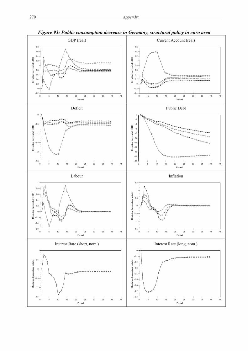
270 Appendix
Figure 93: Public consumption decrease in Germany, structural policy in euro area GDP (real)
-0,2
0
0,2
0,4
0,6
0,8
1
1,2
1,4
1,6
1,8
0 5 10 15 20 25 30 35 40 45
Period
Dev
iatio
n [p
erce
nt o
f GD
P]
Current Account (real)
-0,4
-0,2
0
0,2
0,4
0,6
0,8
1
1,2
1,4
1,6
0 5 10 15 20 25 30 35 40 45
Period
Dev
iatio
n [p
erce
nt o
f GD
P]
Deficit
-2,5
-2
-1,5
-1
-0,5
0
0 5 10 15 20 25 30 35 40 45
Period
Dev
iatio
n [p
erce
nt o
f GD
P]
Public Debt
-20
-18
-16
-14
-12
-10
-8
-6
-4
-2
0
0 5 10 15 20 25 30 35 40 45
Period
Dev
iatio
n [p
erce
nt o
f GD
P]
Labour
-0,6
-0,4
-0,2
0
0,2
0,4
0,6
0,8
1
0 5 10 15 20 25 30 35 40 45
Period
Dev
iatio
n [p
erce
nt o
f GD
P]
Inflation
-1,5
-1
-0,5
0
0,5
1
1,5
0 5 10 15 20 25 30 35 40 45
Period
Dev
iatio
n [p
erce
ntag
e po
ints
]
Interest Rate (short, nom.)
-1,5
-1
-0,5
0
0,5
1
0 5 10 15 20 25 30 35 40 45
Period
Dev
iatio
n [p
erce
ntag
e po
ints
]
Interest Rate (long, nom.)
-0,8
-0,7
-0,6
-0,5
-0,4
-0,3
-0,2
-0,1
0
0 5 10 15 20 25 30 35 40 45
Period
Dev
iatio
n [p
erce
ntag
e po
ints
]

Appendix 271
Figure 94: Public consumption decrease in Italy, structural policy in euro area GDP (real)
-1,5
-1
-0,5
0
0,5
1
1,5
2
2,5
0 5 10 15 20 25 30 35 40 45
Period
Dev
iatio
n [p
erce
nt o
f GD
P]
Current Account (real)
-0,2
0
0,2
0,4
0,6
0,8
1
1,2
1,4
1,6
1,8
0 5 10 15 20 25 30 35 40 45
Period
Dev
iatio
n [p
erce
nt o
f GD
P]
Deficit
-3
-2,5
-2
-1,5
-1
-0,5
0
0,5
0 5 10 15 20 25 30 35 40 45
Period
Dev
iatio
n [p
erce
nt o
f GD
P]
Public Debt
-25
-20
-15
-10
-5
0
5
0 5 10 15 20 25 30 35 40 45
Period
Dev
iatio
n [p
erce
nt o
f GD
P]
Labour
-1,5
-1
-0,5
0
0,5
1
1,5
0 5 10 15 20 25 30 35 40 45
Period
Dev
iatio
n [p
erce
nt o
f GD
P]
Inflation
-2
-1,5
-1
-0,5
0
0,5
1
1,5
2
0 5 10 15 20 25 30 35 40 45
Period
Dev
iatio
n [p
erce
ntag
e po
ints
]
Interest Rate (short, nom.)
-0,4
-0,3
-0,2
-0,1
0
0,1
0,2
0,3
0 5 10 15 20 25 30 35 40 45
Period
Dev
iatio
n [p
erce
ntag
e po
ints
]
Interest Rate (long, nom.)
-0,3
-0,25
-0,2
-0,15
-0,1
-0,05
0
0 5 10 15 20 25 30 35 40 45
Period
Dev
iatio
n [p
erce
ntag
e po
ints
]

272 Appendix
Figure 95: Public consumption decrease and structural policy in euro area GDP (real)
-0,5
0
0,5
1
1,5
2
2,5
0 5 10 15 20 25 30 35 40 45
Period
Dev
iatio
n [p
erce
nt o
f GD
P]
Current Account (real)
0
0,2
0,4
0,6
0,8
1
1,2
1,4
1,6
0 5 10 15 20 25 30 35 40 45
Period
Dev
iatio
n [p
erce
nt o
f GD
P]
Deficit
-3
-2,5
-2
-1,5
-1
-0,5
0
0 5 10 15 20 25 30 35 40 45
Period
Dev
iatio
n [p
erce
nt o
f GD
P]
Public Debt
-25
-20
-15
-10
-5
0
0 5 10 15 20 25 30 35 40 45
Period
Dev
iatio
n [p
erce
nt o
f GD
P]
Labour
-0,6
-0,4
-0,2
0
0,2
0,4
0,6
0,8
1
0 5 10 15 20 25 30 35 40 45
Period
Dev
iatio
n [p
erce
nt o
f GD
P]
Inflation
-1
-0,8
-0,6
-0,4
-0,2
0
0,2
0,4
0,6
0,8
0 5 10 15 20 25 30 35 40 45
Period
Dev
iatio
n [p
erce
ntag
e po
ints
]
Interest Rate (short, nom.)
-2,5
-2
-1,5
-1
-0,5
0
0,5
1
1,5
0 5 10 15 20 25 30 35 40 45
Period
Dev
iatio
n [p
erce
ntag
e po
ints
]
Interest Rate (long, nom.)
-1,4
-1,2
-1
-0,8
-0,6
-0,4
-0,2
0
0 5 10 15 20 25 30 35 40 45
Period
Dev
iatio
n [p
erce
ntag
e po
ints
]

Appendix 273
Figure 96: Tax increase in Germany, structural policy in euro area GDP (real)
0
0,2
0,4
0,6
0,8
1
1,2
1,4
1,6
0 5 10 15 20 25 30 35 40 45
Period
Dev
iatio
n [p
erce
nt o
f GD
P]
Current Account (real)
-0,2
0
0,2
0,4
0,6
0,8
1
1,2
0 5 10 15 20 25 30 35 40 45
Period
Dev
iatio
n [p
erce
nt o
f GD
P]
Deficit
-2,5
-2
-1,5
-1
-0,5
0
0 5 10 15 20 25 30 35 40 45
Period
Dev
iatio
n [p
erce
nt o
f GD
P]
Public Debt
-20
-18
-16
-14
-12
-10
-8
-6
-4
-2
0
0 5 10 15 20 25 30 35 40 45
Period
Dev
iatio
n [p
erce
nt o
f GD
P]
Labour
-0,4
-0,2
0
0,2
0,4
0,6
0,8
0 5 10 15 20 25 30 35 40 45
Period
Dev
iatio
n [p
erce
nt o
f GD
P]
Inflation
-0,8
-0,6
-0,4
-0,2
0
0,2
0,4
0,6
0,8
1
1,2
0 5 10 15 20 25 30 35 40 45
Period
Dev
iatio
n [p
erce
ntag
e po
ints
]
Interest Rate (short, nom.)
-1,2
-1
-0,8
-0,6
-0,4
-0,2
0
0,2
0,4
0,6
0,8
0 5 10 15 20 25 30 35 40 45
Period
Dev
iatio
n [p
erce
ntag
e po
ints
]
Interest Rate (long, nom.)
-0,6
-0,5
-0,4
-0,3
-0,2
-0,1
0
0 5 10 15 20 25 30 35 40 45
Period
Dev
iatio
n [p
erce
ntag
e po
ints
]
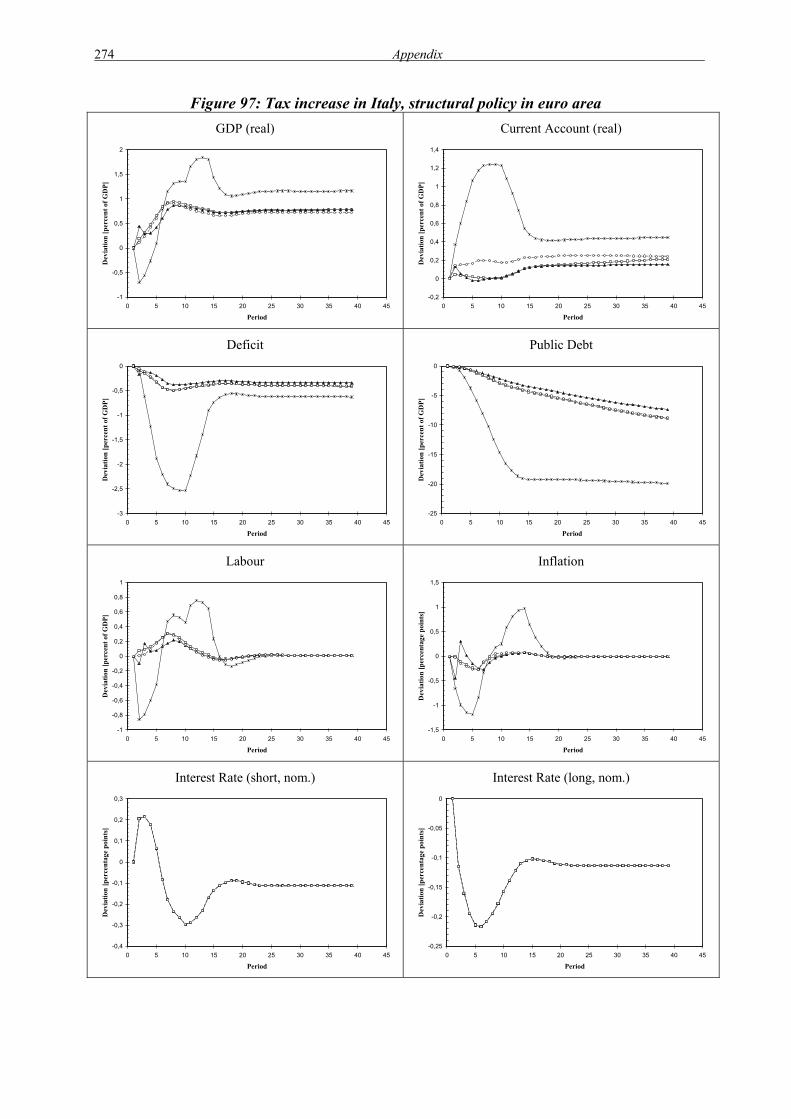
274 Appendix
Figure 97: Tax increase in Italy, structural policy in euro area GDP (real)
-1
-0,5
0
0,5
1
1,5
2
0 5 10 15 20 25 30 35 40 45
Period
Dev
iatio
n [p
erce
nt o
f GD
P]
Current Account (real)
-0,2
0
0,2
0,4
0,6
0,8
1
1,2
1,4
0 5 10 15 20 25 30 35 40 45
Period
Dev
iatio
n [p
erce
nt o
f GD
P]
Deficit
-3
-2,5
-2
-1,5
-1
-0,5
0
0 5 10 15 20 25 30 35 40 45
Period
Dev
iatio
n [p
erce
nt o
f GD
P]
Public Debt
-25
-20
-15
-10
-5
0
0 5 10 15 20 25 30 35 40 45
Period
Dev
iatio
n [p
erce
nt o
f GD
P]
Labour
-1
-0,8
-0,6
-0,4
-0,2
0
0,2
0,4
0,6
0,8
1
0 5 10 15 20 25 30 35 40 45
Period
Dev
iatio
n [p
erce
nt o
f GD
P]
Inflation
-1,5
-1
-0,5
0
0,5
1
1,5
0 5 10 15 20 25 30 35 40 45
Period
Dev
iatio
n [p
erce
ntag
e po
ints
]
Interest Rate (short, nom.)
-0,4
-0,3
-0,2
-0,1
0
0,1
0,2
0,3
0 5 10 15 20 25 30 35 40 45
Period
Dev
iatio
n [p
erce
ntag
e po
ints
]
Interest Rate (long, nom.)
-0,25
-0,2
-0,15
-0,1
-0,05
0
0 5 10 15 20 25 30 35 40 45
Period
Dev
iatio
n [p
erce
ntag
e po
ints
]

Appendix 275
Figure 98: Tax increase and structural policy in euro area GDP (real)
0
0,2
0,4
0,6
0,8
1
1,2
1,4
1,6
1,8
2
0 5 10 15 20 25 30 35 40 45
Period
Dev
iatio
n [p
erce
nt o
f GD
P]
Current Account (real)
0
0,2
0,4
0,6
0,8
1
1,2
0 5 10 15 20 25 30 35 40 45
Period
Dev
iatio
n [p
erce
nt o
f GD
P]
Deficit
-3
-2,5
-2
-1,5
-1
-0,5
0
0 5 10 15 20 25 30 35 40 45
Period
Dev
iatio
n [p
erce
nt o
f GD
P]
Public Debt
-25
-20
-15
-10
-5
0
0 5 10 15 20 25 30 35 40 45
Period
Dev
iatio
n [p
erce
nt o
f GD
P]
Labour
-0,4
-0,2
0
0,2
0,4
0,6
0,8
0 5 10 15 20 25 30 35 40 45
Period
Dev
iatio
n [p
erce
nt o
f GD
P]
Inflation
-0,8
-0,6
-0,4
-0,2
0
0,2
0,4
0,6
0 5 10 15 20 25 30 35 40 45
Period
Dev
iatio
n [p
erce
ntag
e po
ints
]
Interest Rate (short, nom.)
-2
-1,5
-1
-0,5
0
0,5
1
0 5 10 15 20 25 30 35 40 45
Period
Dev
iatio
n [p
erce
ntag
e po
ints
]
Interest Rate (long, nom.)
-1,2
-1
-0,8
-0,6
-0,4
-0,2
0
0 5 10 15 20 25 30 35 40 45
Period
Dev
iatio
n [p
erce
ntag
e po
ints
]

276 Appendix
Figure 99: Public consumption decrease and tax increase in Germany, structural policy in euro area
GDP (real)
-0,5
0
0,5
1
1,5
2
0 5 10 15 20 25 30 35 40 45
Period
Dev
iatio
n [p
erce
nt o
f GD
P]
Current Account (real)
-0,4
-0,2
0
0,2
0,4
0,6
0,8
1
1,2
1,4
1,6
1,8
0 5 10 15 20 25 30 35 40 45
Period
Dev
iatio
n [p
erce
nt o
f GD
P]
Deficit
-2,5
-2
-1,5
-1
-0,5
0
0 5 10 15 20 25 30 35 40 45
Period
Dev
iatio
n [p
erce
nt o
f GD
P]
Public Debt
-20
-18
-16
-14
-12
-10
-8
-6
-4
-2
0
0 5 10 15 20 25 30 35 40 45
Period
Dev
iatio
n [p
erce
nt o
f GD
P]
Labour
-0,8
-0,6
-0,4
-0,2
0
0,2
0,4
0,6
0,8
1
1,2
0 5 10 15 20 25 30 35 40 45
Period
Dev
iatio
n [p
erce
nt o
f GD
P]
Inflation
-1,5
-1
-0,5
0
0,5
1
1,5
0 5 10 15 20 25 30 35 40 45
Period
Dev
iatio
n [p
erce
ntag
e po
ints
]
Interest Rate (short, nom.)
-2
-1,5
-1
-0,5
0
0,5
1
1,5
0 5 10 15 20 25 30 35 40 45
Period
Dev
iatio
n [p
erce
ntag
e po
ints
]
Interest Rate (long, nom.)
-0,9
-0,8
-0,7
-0,6
-0,5
-0,4
-0,3
-0,2
-0,1
0
0 5 10 15 20 25 30 35 40 45
Period
Dev
iatio
n [p
erce
ntag
e po
ints
]

Appendix 277
Figure 100: Public consumption decrease and tax increase in Italy, structural policy in euro area
GDP (real)
-1,5
-1
-0,5
0
0,5
1
1,5
2
2,5
3
0 5 10 15 20 25 30 35 40 45
Period
Dev
iatio
n [p
erce
nt o
f GD
P]
Current Account (real)
-0,5
0
0,5
1
1,5
2
0 5 10 15 20 25 30 35 40 45
Period
Dev
iatio
n [p
erce
nt o
f GD
P]
Deficit
-3
-2,5
-2
-1,5
-1
-0,5
0
0,5
0 5 10 15 20 25 30 35 40 45
Period
Dev
iatio
n [p
erce
nt o
f GD
P]
Public Debt
-25
-20
-15
-10
-5
0
5
0 5 10 15 20 25 30 35 40 45
Period
Dev
iatio
n [p
erce
nt o
f GD
P]
Labour
-1,5
-1
-0,5
0
0,5
1
1,5
0 5 10 15 20 25 30 35 40 45
Period
Dev
iatio
n [p
erce
nt o
f GD
P]
Inflation
-2
-1,5
-1
-0,5
0
0,5
1
1,5
2
0 5 10 15 20 25 30 35 40 45
Period
Dev
iatio
n [p
erce
ntag
e po
ints
]
Interest Rate (short, nom.)
-0,5
-0,4
-0,3
-0,2
-0,1
0
0,1
0,2
0,3
0,4
0 5 10 15 20 25 30 35 40 45
Period
Dev
iatio
n [p
erce
ntag
e po
ints
]
Interest Rate (long, nom.)
-0,3
-0,25
-0,2
-0,15
-0,1
-0,05
0
0 5 10 15 20 25 30 35 40 45
Period
Dev
iatio
n [p
erce
ntag
e po
ints
]

278 Appendix
Figure 101: Public consumption decrease, tax increase and structural policy in euro area GDP (real)
-0,5
0
0,5
1
1,5
2
2,5
3
0 5 10 15 20 25 30 35 40 45
Period
Dev
iatio
n [p
erce
nt o
f GD
P]
Current Account (real)
0
0,2
0,4
0,6
0,8
1
1,2
1,4
1,6
1,8
0 5 10 15 20 25 30 35 40 45
Period
Dev
iatio
n [p
erce
nt o
f GD
P]
Deficit
-3
-2,5
-2
-1,5
-1
-0,5
0
0 5 10 15 20 25 30 35 40 45
Period
Dev
iatio
n [p
erce
nt o
f GD
P]
Public Debt
-25
-20
-15
-10
-5
0
0 5 10 15 20 25 30 35 40 45
Period
Dev
iatio
n [p
erce
nt o
f GD
P]
Labour
-0,8
-0,6
-0,4
-0,2
0
0,2
0,4
0,6
0,8
1
1,2
0 5 10 15 20 25 30 35 40 45
Period
Dev
iatio
n [p
erce
nt o
f GD
P]
Inflation
-1
-0,8
-0,6
-0,4
-0,2
0
0,2
0,4
0,6
0,8
0 5 10 15 20 25 30 35 40 45
Period
Dev
iatio
n [p
erce
ntag
e po
ints
]
Interest Rate (short, nom.)
-3
-2,5
-2
-1,5
-1
-0,5
0
0,5
1
1,5
2
0 5 10 15 20 25 30 35 40 45
Period
Dev
iatio
n [p
erce
ntag
e po
ints
]
Interest Rate (long, nom.)
-1,6
-1,4
-1,2
-1
-0,8
-0,6
-0,4
-0,2
0
0 5 10 15 20 25 30 35 40 45
Period
Dev
iatio
n [p
erce
ntag
e po
ints
]

Appendix 279
Appendix 6: Variables used in chapter 6
Acronym Definition Description Source Maximum time span
Minimum time span
UR Unemployment rate Unemployment rate Nickell and Nunziata, 2001; EUROSTAT Euroindicators
1960 - 2004 1975 - 2004
EMP Employment Total employment OECD, Economic Outlook 1960 - 2004 1969 - 2004
MARKUP Mark-up Mark-up of prices over cost own calculations 1970 - 2004 1977 - 2004
PROD Labour productivity Real GDP over employees own calculations 1960 - 2004 1969 – 2004
GTRENDPROD Trend labour productivity Growth rate of Hodrick-Prescott filtered labour productivity (PROD)
own calculations 1961 - 2004 1970 - 2004
GTFP TFP growth (Solow residual) Annual growth rate to total factor productivity own calculations 1961 - 2004 1977 - 2004
BRR Benefit replacement rate Benefit in the first year of unemployment, as a percentage of earnings before tax
Nickell and Nunziata, 2001; Nickell 2003
1960 - 1999 1975 - 1999
BD Benefit duration Index; weighted average between ratio of BRR in 2nd year to BRR in 1st year and ratio of BRR in 4th year to BRR in 1st year
Nickell and Nunziata, 2001; Nickell 2003
1960 - 1999 1975 - 1999
CO Bargaining coordination Index {1,3}, increasing in degree of coordination in the bargaining process on the employers' and the unions' side
Nickell and Nunziata, 2001; Nickell 2003
1960 - 1998 1975 - 1998
LREG Labour market regulation Index (1;10), decreasing in regulation Fraser Institute 1970 - 2002 1975 - 2002
SUB Subsidies Transfers and subsidies as a percentage of GDP Fraser Institute 1970 - 2002 1975 - 2002

280 References
References
van Aarle, B. and H. Garretsen (2003), Keynesian, Non-Keynesian or No Effects of Fiscal
Policy Changes? The EMU Case, Journal of Macroeconomics, vol. 25, pp. 213-240.
Afonso, A. (2001), Non-Keynesian Effects of Fiscal Policy in the EU-15, unpublished paper,
May.
Afonso, A. and R. Strauch (2003), Fiscal policy events and interest rate swaps spreads: some
evidence from EU, ECB working paper no. 303.
Ahmed, S., B. Ickes, P. Wang and B. Sam Yoo (1993), International Business Cycles,
American Economic Review, vol. 83, no. 3, pp.335-359.
Ahn, S. (2002), Competition, Innovation and Productivity Growth: A Review of Theory and
Evidence, OECD Economics Department Working Papers no.317.
Alesina A. and S. Ardagna (1998), Tales of Fiscal Adjustment, Economic Policy, vol. 13, no.
27, pp. 487-545.
Alesina, A., S. Ardagna, G. Nicoletti and F. Schiantarelli (2003), Regulation and Investment,
OECD Economics Department Working Papers no.352.
Alesina, A.; M. de Broeck; A. Prati and G. Tabellini (1992), Default risk on government debt
in OECD countries, Economic Policy, vol. 15, pp. 427-463.
Allsopp, Ch., W. J. McKibbin and D. Vines (1999), Fiscal Consolidation in Europe: Some
Empirical Issues, in A. Hughes Hallett et al. (1999), pp. 288–333.
Ardagna, S. (1999), Fiscal stabilizations: When do they work and why, unpublished paper,
July.
Ardagna, S.; F. Caselli and T. Lane (2005), Fiscal discipline and the cost of public debt
service: some estimates for OECD countries, Centre for Economic Performance, CEP
Discussion Paper No. 670.
Artis, M.; H.-M. Krolzig and J. Toro (1998), The European Business Cycle, CEPR Discussion
Paper No. 2242.
Badinger, H. (2004), Do we really know that the EU’s Single Market Programme has fostered
competition? Testing for a decrease in markup ratios in EU industries. Europainstitut,
Wirtschaftsuniversität Wien, Working Paper 55.

Appendix
Barth, J., G. Iden; F. Russek and M. Wohar (1991), The Effects of Federal Budget Deficits on
Interest Rates and the Composition of Domestic Output, in: Penner, R. (ed.), The great
fiscal experiment, Washington D.C.: Urban Institute Press, pp. 69-141.
Bayoumi, T. and B. Eichengreen (1992), Shocking Aspects of European Monetary
Integration. In F. Torres and F. Giavazzi (eds.), Adjustment and Growth in the European
Monetary Union. Cambridge University Press, 1993, p.193-229.
Bayoumi, T.; M. Goldstein and G. Woglom (1995), Do credit markets discipline sovereign
borrowers? Evidence from the US States, Journal of Money, Credit and Banking, vol.27,
no. 4, pp.1046-1059.
Bayoumi, T., D. Laxton, and P. Pesenti (2004), Benefits and Spillovers of Greater
Competition in Europe: A Macroeconomic Assessment, NBER Working Paper 10416.
Bayoumi T. and P. Masson (1998), Liability-creating versus non-liability-creating fiscal
stabilisation policies: Ricardian equivalence, fiscal stabilisation and EMU, The Economic
Journal, vol. 108, pp. 1026-1045.
Beetsma, R. and L. Bovenberg (1999), Does monetary unification lead to excessive debt
accumulation?, Journal of Public Economics, vol. 74, pp. 299-325.
Beetsma, R. and M. M. Giuliodori (2004), What are the spillovers from fiscal shocks in
Europe? An empirical analysis, ECB working paper no. 325.
Beetsma, R. and H. Jensen (2002), Monetary and fiscal policy interactions in a micro-founded
model of a monetary union, ECB working paper no. 166.
Beetsma, R.; M. Giuliodori and F. Klaassen (2005), Trade Spillovers of Fiscal Policy in the
European Union: A Panel Analysis, mimeo, University of Amsterdam.
Bernanke, B. and A. Blinder (1992), The Federal Funds Rate and the Channels of Monetary
Transmission, American Economic Review, vol.82 (4), pp.901-921.
Bernheim, D. (1987), Ricardian equivalence: an evaluation of theory and evidence, in:
FISCHER S. (ed.), NBER Macroeconomics Annual, Cambridge: MIT Press, p. 263-304.
Bertola, G. and A. Drazen (1993), Trigger points and budget cuts: explaining the effects of
fiscal austerity, American Economic Review, vol. 83, no. 1, March, pp. 11-26.
Blanchard, O. (1990), A Traditional Interpretation of Macroeconomic Fluctuations, American
Economic Review, vol.79, no. 5, pp.1146-1164.

282 References
Blanchard, O. and R. Perotti (2002), An empirical characterisation of the dynamic effects of
changes in government spending and taxes on output, Quarterly Journal of Economics,
vol. 117, no.4, pp. 1329-1368.
Blanchard, O. and F. Giavazzi (2001), Macroeconomic effects of regulation and deregulation
in goods and labour markets, NBER Working Paper 8120.
Blanchard, O. and D. Quah (1989), The Dynamic Effects of Aggregate Demand and
Aggregate Supply Shocks, American Economic Review, vol.79, no. 4, pp.655-673.
Bohn, H. (1998), The behaviour of US public debt and deficits, Quarterly Journal of
Economics, vol. 113(3), p. 949-963.
Brook, A. (2003), Recent and prospective trends in real long-term interest rates: fiscal policy
and other drivers, OECD Economics Department working paper no. 21.
Bruneau, C. and O. De Bandt (2003), Monetary and Fiscal Policy in the Transition to
Monetary Union: What Do SVAR Models Tell Us?, Economic Modelling, vol. 20,
pp.959-985.
Buti, M, W. Roeger and J. in ‘t Veld (2001), Stabilising Output and Inflation in EMU: Policy
Conflicts and Co-operation under the Stability Pact, mimeo.
Calmfors, L. and J. Driffill (1988), Centralization of wage bargaining; Economic Policy 2, 14-
61.
Canova, F. and H. Dellas (1993), Trade Interdependence and the International Business
Cycle, Journal of International Economics, vol.34, pp.23-47.
Canzoneri, M.; R. Cumby and B. Diba (2001), Fiscal Discipline and Exchange Rate Regimes,
Economic Journal, vol. 111, pp. 667-690.
Caporale, G., and G. Williams (2002), Long-term nominal interest rates and domestic
fundamentals, Review of Financial Economics, vol. 11, p. 119-130.
Cebula, R. (1998), An Empirical Analysis of the Impact of Federal Budget Deficits on Long-
Term Nominal Interest Rate Yields: Using Alternative Expected Inflation Measures,
Review of Financial Economics, vol. 7, no. 1, pp. 55-64.
Cebula, R. and J.V. Koch (1989), An empirical note on deficits, interest rates, and
internaiional capital flows, Quarterly Review of Economics and Business, vol. 29(3), p.
121-127.

Appendix
Claeys P. (2004), Monetary and Budgetary Policy Interaction: An SVAR Analysis of
Stabilization Policies in Monetary Union, EUI working paper, no. 22.
Cochrane, J. (2001), Long term debt and optimal policy in the FTPL, Econometrica, vol. 69,
pp. 69-116.
Codogno, L.; C. Favero and A. Missale (2003), Yield spreads on EMU government bonds,
Economic Policy, pp. 503-532.
Conway. P. and A. Orr (2002), The GIRM: a global interest rate model, Westpac Institutional
Bank Occasional Paper.
Coppens, F. and D. Vivet (2004), Liberalisation of network industries: Is the eledtgricity
sector an exception to the rule?, National Bank of Belgium, Working Paper 200409.
Dalamagas, B. (1993), Fiscal effectiveness and debt illusion in a rational expectations model,
Annales d’Economie et de Statistique, no. 31, September, pp. 129-146.
Dalsgaard, T. and A. de Serres (2000), Estimating Prudent Budgetary Margins for EU
Countries: A Simulated SVAR Model Approach, OECD Economic Studies, vol. 30, no. 1,
pp.115-147.
Daniel, B. (2001), The fiscal theory of the price level in an open economy, Journal of
Monetary Economics, vol. 48, pp. 293-308.
De Arcangelis, G. and S. Lamartina (2004), Fiscal shocks and policy regimes in some OECD
countries, in: Beetsma et al. (eds.), Fiscal policies, monetary policies and labour markets,
Key aspects of European macroeconomic policies after monetary unification, Cambridge:
Cambridge University Press, pp. 224-255.
De Grauwe, P. (1999), Discussion of Allsopp et al., 1999, in Andrew Hughes Hallett et al.
(1999), Fiscal Aspects of European Monetary Integration, pp. 334–345.
Di Bartolomeo, G.; J. Engwerda; J. Plasmans, B; van Aarle and T. Michalak (2005),
Macroeconomic Stabilization Policies in the EMU: Spillovers, Asymmetries, and
Institutions, CESifo Working Paper No. 1376.
Drudi, F. and A. Prati (2000), Signaling Fiscal Regime Sustainability, European Economic
Review, vol. 44(10), p. 1897-1930.
Dupor B. (2000), Exchange rates and the fiscal theory of the price level, Journal of Monetary
Economics, vol. 45, pp. 613-630.

284 References
Elmendorf, D. (1993), Actual budget deficit expectations and interest rates, Harvard Institute
of Economic Research.
Elmendorf, D. (1996), The effect of deficit reduction laws on real interest rates, Federal
Reserve Board.
Elmendorf, D. and N. Mankiw (1999), Government debt, in: Taylor, J. and M. Woodford, M.
(eds.), Handbook of Macroeconomics, Amsterdam: Elsevier Science, Chapter 25.
Eengen, E. and G. Hubbard (2004), Federal government debt and interest rates, NBER
working paper no. 10681.
Estevao, M. (2004), Why is Productivity Growth in the euro area so sluggish? IMF Working
Paper WP/04/200.
European Commission (2004), The EU Economy: 2004 Review, European Economy no. 6.
Evans, P. (1987a), Interest rates and expected future budget deficits in the US, Journal of
Political Economy, vol. 95, no. 1.
Evans, P. (1987b), Do budget deficits raise nominal interest rates? Evidence from six
countries, Journal of Monetary Economics, vol. 20, pp. 281-300.
Evans, P. and D. Marshall (2002), Economic determinants of the nominal Treasury yield
curve, Federal Reserve Bank of Chicago, working paper no. 16.
Fagan, G., J. Henry and R. Mestre (2001), An Area-Wide Model (AWM) for the Euro Area,
ECB working paper no. 42.
Faini, R. (2005), Fiscal policy and interest rates in Europe, mimeo, University Tor Vergata.
Fatas, A. and I. Mihov (1999), The Macroeconomic Effects of Fiscal Policy, mimeo.
Favero, C. (2003), How do European monetary and fiscal authorities behave?, in: Buti, M.
(ed.), Monetary and fiscal policies in EMU: interactions and coordination, Cambridge:
Cambridge University Press, pp. 217-245.
Favero, C.; F. Giavazzi and L. Spaventa (1997), High yields: the spread on German interest
rates, Economic Journal, vol. 107, pp. 956-985.
Feldstein, M. (1986), Budget deficits, tax rules and real interest rates, NBER working paper
no. 1970.
Ford, R. and D. Laxton (1995), World public debt and real interest rates, IMF working paper
no. 30.

Appendix
Gale, W. and P. Orszag (2002), The economic effects of long-term fiscal discipline,
Brookings Institution.
Garcia, S. and A. Verdelhan (1999), Impact of the Monetary and Fiscal Shocks in the Euro
Area, mimeo.
Garcia, S. and P. Hénin (2000), Balancing Budget Through Tax Increases or Expenditure
Cuts: Is it Neutral? Economic Modelling, vol. 16, pp.591-612.
Gerlach, S. and F. Smets (1995), The Monetary Transmission Mechanism: Evidence from the
G7 Countries, BIS Discussion Paper no.26.
Giavazzi, F. and M. Pagano (1990), Can severe fiscal contractions be expansionary? Tales of
two small European countries, NBER Macroeconomics Annual, pp. 75-111.
Giordani, P. (2004), Evaluating New-Keynesian models of a small open economy, Oxford
Bulletin of Economics and Statistics, vol. 66, Special Issue, pp. 713-733.
Gjersem, C. (2004), Policies Bearing on Product Market Competition and Growth in Europe,
OECD Economics Department Working Papers no.378
Gobbin, N. and B. van Aarle (2001), Fiscal adjustments and their effects during the transition
to EMU, Public Choice, vol. 109, no. 3-4, pp. 269-299, December.
Gordon, D. and E. Leeper (1994), The Dynamic Impacts of Monetary Policy: An Exercise in
Tentative Identification, Journal of Political Economy, vol.102(6), pp.1228-1247.
Griffith, R. and R. Harrison (2004), The link between product market reform and macro-
economic performance, European Commission, Economic Papers no.209.
Gwartney, J. and R. Lawson (2004), Economic Freedom of the World: 2004 Annual Report,
Fraser Institute, Vancouver, http://www.freetheworld.com.
Haber, G.; R. Neck and W.J. McKibbin (2006), Less Government – More Wealth? On the
Macroeconomics of a Smaller Public Sector in Europe. Forthcoming in: International
Advances in Economic Research 12, no. 1.
Hansen, B.E. (1997): Inference in TAR models, Studies in Nonlinear Dynamics and
Econometrics, vol. 2, no. 1, pp. 1-14, April.
Hansen, B.E. (1999): Threshold effects in non-dynamic panels: Estimation, testing, and
inference, Journal of Econometrics, vol. 93, pp. 345-368.

286 References
Hansen, B.E. (2000): Sample Splitting and Threshold Estimation, Econometrica, vol. 68, no.
3, pp. 575-603.
Heylen, F. and G. Everaert (2000), Success and failure of fiscal consolidation in the OECD: a
multivariate analysis, Public Choice, no. 105, pp. 103-124.
Hogan, V. (2004): Expansionary Fiscal Contractions? Evidence from panel data,
Scandinavian Journal of Economics, vol. 106, no. 4, pp. 647-659.
Höppner, F. and K. Wesche (2000): Non-linear effects of fiscal policy in Germany: A
Markov-switching approach, Bonn Economic Discussion Papers, no. 2000/9.
Hughes Hallett, A.; P. Mooslechner and M. Schuerz (eds.) (2001), Challenges for Economic
Policy Coordination within European Monetary Union, Boston: Kluwer.
IMF (2003), Unemployment and labour market institutions: why reforms pay off; April
World Economic Outlook.
Jean, S. and G. Nicoletti (2002), Product Market Regulation and Wage Premia in Europe and
North America: An Empirical Investigation, OECD Economics Department Working
Papers no.318.
Judson, R.A. and A.L. Owen (1999): Estimating dynamic panel data models: a guide for
macroeconomists, Economics Letters, 65, pp. 9-15.
McKibbin, W.J. and J.D. Sachs (1991), Global Linkages, Washington, DC: Brookings
Institution.
McKibbin, W.J. and P. Wilcoxen (1998), The Theoretical and Empirical Structure of the G-
Cubed model, Brookings Discussion Paper in International Economics no. 118.
Kim, S. (1999), Do Monetary Policy Shocks Matter in the G-7 Countries? Using Common
Identifying Assumptions about Monetary Policy across Countries, Journal of International
Economics, vol.48, pp.387-412.
Kim, S. (2001), Effects of Monetary Policy Shocks on the Trade Balance in Small Open
European Countries, Economic Letters, vol.71, pp.197-203.
Kim, S. and N. Roubini (2000), Exchange Rate Anomalies in the Industrial Countries: A
Solution with a Structural VAR Approach, Journal of Monetary Economics, vol.45,
pp.561-586.

Appendix
Kitchen, J. (1996), Domestic and International Financial Market Responses to Federal Deficit
Announcements, Journal of International Money and Finance, vol. 15, pp. 239-254.
Kitchen, J. (2002), A note on interest rates and structural budget deficits, mimeo.
Knot, K. (1996), Fiscal policy and interest rates in the European Union, Cheltenham: Edward
Elgar Publishing.
Koren, S. and A. Stiassny (1998), Tax and Spend, or Spend and Tax? An International Study,
Journal of Policy Modeling, vol.20, no.2: pp.163-191.
Landon, S. and C. Smith (2000), Government debt spillovers and creditworthiness in a
federation, The Canadian Journal of Economics, vol. 33, no.3, pp. 364-661.
Laubach, T. (2003), New evidence on the interest rate effects of budget deficits and debt,
mimeo, Board of Governors of the Federal Reserve System.
Leeper, E., C. Sims and T. Zha (1996), What Does Monetary Policy Do? Brookings Papers on
Economic Activity, vol.1996, no.2, pp.1-63.
Linde, J. (2001), Fiscal policy and interest rates in a small open economy, Finnish Economic
Paper, vol. 14(2).
Marcellino, M. (2002), Some stylised facts on non-systematic fiscal policy in the Euro-area,
CEPR discussion paper no. 3635.
Martins, J.O., S. Scarpetta and D. Pilat (1996), Mark-up Ratios in Manufacturing Industries.
Estimates for 14 OECD Countries. OECD Economics Department Working Paper
no. 162.
Mehra, Y. (2001), The bond rate and estimated monetary policy rules, Journal of Economics
and Business, vol. 53, no.4, pp. 345-358.
Mélitz, J. (2000), Some Cross-Country Evidence about Fiscal Policy Behavior and
Consequences for EMU, mimeo.
Miller, S. and F. Russek (1996), Do Federal Deficits Affect Interest Rates? Evidence from
Three Econometric Methods, Journal of Macroeconomics, vol. 18, no.3, pp. 403-428.
Muscatelli, A.; P. Tirelli and C. Trecroci (2002), Monetary and Fiscal Policy Interactions over
the Cycle: Some Empirical Evidence, CESifo Working Paper no.817.
Neck, R: and F. Schneider (eds.) (2001), The Political Economy of Fiscal Policies, Special
Issue of Public Choice, Vol. 109, no. 3-4.

288 References
Nickell, S. (1981), Biases in dynamic models with fixed effects, Econometrica, vol. 49, no. 6,
pp. 1417-1426.
Nickell, S. (2003), Labour Market Institutions and Unemployment in OECD Countries,
CESifo DICE Report 2/2003, 13-26.
Nickell, S. and L. Nunziata (2001), Labour market institutions database, vers. 2.00, LSE,
Centre of Economic Performance; http://cep.lse.ac.uk/pubs/download/data0502.zip.
Nunziata, L. (2001), Institutions and Wage Determination: a Multi-Country Approach,
University of Oxford, Nuffield College, Working Paper 2001-W29.
O’Donovan, B.; A. Orr and D. Rae (1996), A world interest rate model, National Bank of
New Zealand, Financial Research Paper no. 7.
Orr, A.; M. Eedey and M. Kennedy (1995), The determinants of real long-term interest rates:
17 country pooled time series evidence, OECD working paper no. 155.
Paesani, P.; R. Strauch, and M. Kremer (2005), Public debt and long-term interest rates: the
case of Germany, Italy and the USA, mimeo, European Central Bank.
Perotti, R (1999), Fiscal policy in good times and bad, Quarterly Journal of Economics,
November, pp. 1399-1436.
Prasad, E. and R. Lumsdaine (2003), Identifying the common component of international
economic fluctuations: a new approach, Economic Journal, vol. 113, pp. 101-127.
Prozybyla, M. and M. Roma (2005), Does Product Market Competition reduce Inflation?
Evidence from EU Countries and Sectors, ECB Working Paper No. 453.
Ramey, V. and M. Shapiro (1998), Costly capital reallocation and the effects of government
spending, Carnegie Rochester Conference on Public Policy, vol. 48, pp. 145-194.
Reinhart, V. and B. Sack (2000), The economic consequences of disappearing government
debt, Brookings Papers on Economic Activity, vol. 2, pp. 163-209.
Roeger, W. (1995), Can imperfect Competition explain the Difference between Primal and
Dual Productivity Measures? Estimates for US manufacturing. Journal of Political
Economy, vol. 103, no. 2.
Rogoff, K. (1985), Can International Monetary Policy Cooperation be Counterproductive?
Journal of International Economics, vol. 18, pp. 199–217.

Appendix
Rowley, Ch. K.; W.F. Shughart II and R.D. Tollison D. (2002) (eds.) The Economics of
Budget Deficits, 2 vols., Cheltenham: Edward Elgar.
Rudebusch, G. (1998), Do Measures of Monetary Policy in a VAR Make Sense?,
International Economic Review, vol.39, no.4, pp.933-940.
Sala, L. (2004), The Fiscal Theory of the Price Level: identifying restrictions and empirical
evidence, IGIER working paper no. 257.
Sauner-Leroy, J.-B. (2003), The impact of the implementation of the Single Market
Programme on productive efficiency and the mark-ups in the European Union
manufacturing industry, European Economy, Economic Papers No. 192.
Semmler, W. and W. Zhang (2004), Monetary and Fiscal Policy Interactions in the Euro
Area, Empirica, vol. 31, pp. 205-227.
Sims, C. (1992), Interpreting the Macroeconomic Time Series Facts: The Effects of Monetary
Policy, European Economic Review, vol.36, no.5, pp.975-1000.
Sutherland, A. (1995), Fiscal crisis and aggregate demand: can high public debt reverse the
effects of fiscal policy, CEPR DP no. 1246, September.
Tanzi, V. and M. Lutz (1993), Interest rates and government debt: are the linkages global
rather than national?, in: Verbon, H. and F. van Winden, The political economy of
government debt, Amsterdam: Elsevier Science, pp. 233-253.
Tavares, J. and R. Valkanov (2001), The neglected effect of fiscal policy on stock and bond
returns, mimeo, UCLA.
Wachtel, P. and J. Young (1987), Deficit announcements and interest rates, American
Economic Review, vol. 77, pp. 1007-1012.
Zaghini, A. (1999), The economic policy of fiscal consolidation: the European experience,
Banca d’Italia, Termi di Discussione, no. 355, June.


