Tellus (2004), 56B, 105–117 Copyright C© Blackwell Munksgaard, 2004

Printed in UK. All rights reserved T E L L U S

Eddy correlation measurements of aerosoldeposition to grass

By RICHARD J . VONG 1∗, DEAN VICKERS 1 and DAVID S. COVERT 2, 1College of Oceanic andAtmospheric Sciences, Oregon State University, Corvallis, OR, 97331-5503, USA; 2Department of Atmospheric

Sciences, University of Washington, Seattle, WA 98195, USA

(Manuscript received 2 January 2003; in final form 4 December 2003)

ABSTRACTAn experiment was conducted to measure aerosol turbulent fluxes to a grass field. A new high-flow-rate aerosol sensorwas deployed from a tower to make eddy correlation (EC) measurements of aerosol turbulent flux and depositionvelocity. The EC data were screened and analysed for uncertainties associated with advection, boundary layer growth,instrument separation and counting particles. An apparent bias in the aerosol flux due to particle hygroscopic growth wasevaluated from chemical and microphysical measurements and removed from the results based on derived corrections.The resulting aerosol deposition velocity for 0.52 µm diameter particles depended on atmospheric stability with valuesof 0.3 cm s−1 during near-neutral stability, 0.44 cm s−1 during unstable periods and 0.16 cm s−1 during stable periodswith an estimated uncertainty of ±0.07 cm s−1 due to chemical composition and particle counting.

1. Introduction

Aerosol turbulent flux and dry deposition have been difficult tomeasure and interpret because a large number of controlling andconfounding factors can contribute to observed fluxes. Thesefactors include effects that are related to boundary layer dynam-ics and aerosol microphysics as well as limitations in the fluxmeasurement technique.

Aerosol deposition is influenced by particle, vegetation andatmospheric boundary layer characteristics. Particles with diam-eters between 0.1 and 1 µm are typically removed by impactionand interception onto the fine structural elements of vegetationafter transport by turbulent eddies. Aerosol flux measurementsalso are influenced by horizontal advection of aerosol emittedby upwind sources (Slinn, 1983) and entrainment of air fromaloft (Businger, 1986); these processes can result in a verticaldivergence of the aerosol flux such that deposition to the under-lying surface is not equivalent to the flux at the measurementheight (section 1.1). Aerosol concentration (for particles in afixed diameter interval) is not typically a conservative propertyin that many particles undergo hygroscopic growth, or shrink-age, during transport through the boundary layer; this processcan produce fluxes (Fairall, 1984; Businger, 1986) that dependon humidity (section 1.2) as much as on particle transport byturbulence. The eddy correlation (EC) technique for measuring

∗Corresponding author.e-mail: vong@coas.oregonstate.edu

fluxes has uncertainties that depend on the number of particlescounted; these counting errors can be large when commercialinstrumentation is used (Fairall, 1984).

Here we describe simultaneous observations of aerosol fluxesthat were obtained using the EC micrometeorological technique.The factors influencing measured aerosol deposition to the un-derlying grass field were addressed by: (a) deploying a new high-flow-rate optical instrument to increase particle counting rate,(b) locating the field site in flat terrain and away from upwindemission sources to minimize advection, (c) utilizing data selec-tion criteria to avoid time periods with advection or boundarylayer growth, (d) measuring aerosol chemical and microphysicalproperties, (e) measuring heat and vapour fluxes and (f) derivingand applying corrections to quantify the effect of hygroscopicgrowth on the observed aerosol flux.

It is convenient and useful to describe aerosol turbulent fluxin terms of an aerosol turbulent deposition velocity

Vdt = w′ N′/N (1)

where N is the 30 min mean aerosol number concentration withina fixed diameter interval (in particles cm−3) (note that all “over-bars” denote mean quantities, usually over 30 min); N ′ is theinstantaneous deviation of a 10 Hz measurement from meanaerosol number concentration (all primed variables are 10 Hzdeviations from the mean); w′ is the instantaneous deviation ofthe vertical wind velocity from its mean (w; positive values forw and w′ are directed upwards, away from the surface); andw′ N ′ is the assembly average vertical velocity–aerosol number

Tellus 56B (2004), 2 105

106 R. J . VONG ET AL.

concentration covariance within a fixed diameter interval, i.e. theEC aerosol turbulent flux.

Vdt can be thought of as a ‘mean-scaled’ turbulent flux and alsocan be calculated in terms of aerosol mass or spectral density ineq. (1). The aerosol size distribution is often described usinga power law (Junge, 1963) where the number concentration ofparticles (in some diameter interval �D, i.e. aerosol spectraldensity dN/ dD) is related to the mean diameter (D) in the intervalas

N = dN/dD = cD−(β+1) (2)

where β is the Junge power-law exponent and c is a site-specificconstant.

In this study we use β to relate measurements of aerosol num-ber concentration at two adjacent diameters because it is ana-lytically convenient (see Appendix A). While this power lawdoes not characterize the aerosol number–size distribution wellover a large size range, it is applicable to the limited size rangesconsidered in this study (e.g. using four separate values of β,one for each aerosol flux, for portions in the interval: 0.3 µm <

diameter < 1.0 µm; see Table 3).Hygroscopic growth and shrinkage of atmospheric aerosol

will affect particle diameter and, thus, measurements of theirbehavior in the turbulent boundary layer. Water-soluble aerosolparticles swell to approximately twice their “dry” diameter as rel-ative humidity (RH) increases to 90%; this “hygroscopic growth”phenomenon is fast enough (Keith and Arons, 1954) that mostparticle sizes may be considered to be nearly in equilibrium withthe local RH (Fairall, 1984). Swietlicki et al. (2000) used em-pirical expressions to characterize the hygroscopic behaviour ofatmospheric aerosol particles on the basis of parameters that aremeasured directly for ambient aerosol or modelled for specificchemical compositions. This relationship between the particlediameter at ambient water vapour saturation ratio D(S) and thedry diameter D0 is

D(S)/D0 = (1 − S)−γ (3)

where γ is a hygroscopic growth parameter that depends onchemical composition and S is the water vapour saturation ratio(S = RH/100%).

Experimental data (Swietlicki et al., 2000) suggested a valuefor γ of 0.214 for “aged European air” of mixed continental–anthropogenic origin with larger values for γ when marineaerosols were characterized.

1.1. Budget equation for aerosol turbulent fluxes

In order that aerosol flux measured from a tower will also de-scribe aerosol deposition to an underlying vegetated surface (i.e.w′ N ′ is constant with height), the conservation equation (Stull,1988) states that aerosol advection and time change (also termed“storage”) must either be absent or that these terms must can-cel. Equation (4) presents the 2-D balance between the timechange (term 1 on the left-hand side (l.h.s.)), horizontal stream-

wise advection (term 2 on the l.h.s.), and vertical divergence ofthe turbulent flux (term 4 on the l.h.s.) that occurs when stream-wise turbulent diffusion (term 3 on the l.h.s.), Brownian diffusion(term 1 on the r.h.s.), divergence of gravitational settling (term2 on the r.h.s.) and aerosol sources (S) are all negligible or inbalance:

∂ N/∂t + ∂(uN )/∂x + ∂(u′ N ′)/∂x + ∂(w′ N ′)/∂z

= D(∂2 N/∂z2) − ∂(vg N )/∂z + S. (4)

In this equation N is mean aerosol number concentration in a spe-cific, fixed, diameter interval, u is wind speed along the stream-wise horizontal direction, vg is sedimentation velocity, D is theparticle Brownian diffusion coefficient for a particular diame-ter, S is any in situ source of aerosol (coagulation, nucleation,emission), x is the streamwise horizontal coordinate, and z is thevertical coordinate (in a rotated coordinate system; see belowand section 3).

Equation (4) illustrates why one would not estimate surfacedeposition for time periods when an aerosol source was locatedupwind (horizontal advection) or when aerosol concentrationis changing substantially (time change, i.e. “non-stationarity”)because vertical divergence in the aerosol flux is likely. Unfor-tunately, these conditions frequently occur such that many ECstudies of aerosol flux will not provide quantitative estimates ofdeposition to terrestrial ecosystems unless the impacts of terms1 and 2 cancel (Slinn, 1983; Businger, 1986). In the absenceof vertical flux divergence, the measured turbulent flux is theaerosol deposition to the underlying surface.

1.2. Effect of heat and vapour fluxes on aerosolturbulent flux

Turbulent heat and vapour vertical fluxes introduce a net mass,or density, flux for a scalar even when the vertical velocity is zerofor the averaging period. This correction (Webb et al., 1980) ac-counts for the differences between an appropriate assumptionthat there is no net mass flux of air into the ground and its usualapplication as, instead, assuming a zero mean vertical velocityduring any flux averaging period (30 min here). These two as-sumptions are equivalent only when there is no heat or vapourflux because density will vary with height due to temperatureand/or vapour gradients. The Webb, or density flux, correction(Businger, 1986) is in the form of a calculated vertical velocity(w), that is

w = 1.61(w′ρH20′/ρair)(1 + 1.61q)(w′T ′/T ) (5)

where ρH2O is the density of water vapour, ρ air is the densityof dry air, q is the specific humidity = ρH2O/ρ air, T is the meanambient air temperature, 1.61 is the ratio of molecular weights ofdry air and water vapour, w′T ′ is the assembly average kinematicturbulent heat flux measured by EC, w′ρH20

′ is the assemblyaverage water vapour turbulent flux measured by EC and w isthe net 30-min vertical velocity that is needed to compensate for

Tellus 56B (2004), 2

EDDY CORRELATION MEASUREMENTS OF AEROSOL DEPOSITION TO GRASS 107

the density flux (coordinate rotations to EC covariances set anyother w to zero).

This ‘density flux correction’ is usually introduced (Hum-melshoj, 1994) as a second term in the flux equation:

F = w′ N ′ + wN . (6)

The calculated mean vertical velocity (w) is analogous to asecond component of aerosol flux (term 2 on the r.h.s. of eq. (6))that is added to that (term 1 on the r.h.s.) which was determinedby EC. This density correction applies to any turbulent flux.

Hygroscopic growth represents a second dependence ofaerosol flux on heat and vapour fluxes beyond the density correc-tion (above). A saturation ratio turbulent flux is defined to helpaccount for the change in the state of hydration of the aerosol asit is transported through an S gradient by near-surface turbulence(Fairall, 1984; Buzorius et al., 2000; Kowalski, 2001) as

w′S′ = w′q ′/qsat − w′T ′(SLv)/(

RvT 2)

(7)

where q sat is the mean saturation value of the specific humidity,S is the mean ambient air saturation ratio (q/qsat), w′q ′ is thewater vapour turbulent flux (vertical velocity–specific humiditycovariance), Lv is the latent heat of vaporization of water and Rv

is the gas law constant for water vapour.Corrections to aerosol turbulent fluxes for hygroscopic growth

of particles are necessary when aerosol size at ambient RH is usedto define N and, thus, the eddy flux. Previous derivations of thesecorrections by Fairall (1984) and Kowalski (2001) have beenmodified here (see Appendix A) to incorporate the Swietlickiet al. (2000) hygroscopic growth factor, γ , which is more easilymeasured in the field or estimated from lab data than is their em-pirical factor (Kf ). Equation (8) provides an appropriate correc-tion (�Vd) to the aerosol deposition velocity that is proportionalto the exponent of the aerosol power-law size distribution (β), thehumidity growth factor (γ ) and the saturation ratio flux (w′S′)but the correction is inversely proportional to the saturation ratiodeficit (1 − S):

�Vdt = −βγw′S′/(1 − S). (8)

Upward saturation ratio fluxes (w′S′ > 0 are typical of wetsoils underlying drier air) induce an apparent upward componentto the aerosol flux and deposition velocity. This humidity cor-rection produces a more downward aerosol flux (more negative)than is directly observed by EC measurements (the correctionhas the opposite sign from w′S′ for the usual case where β > 0).In the absence of any surface removal of particles, eq. (8) statesthat an EC system based on aerosol concentration at ambient RHwould observe an apparent (false) value of Vdt that is equal tothe quantity βγw′S′/(1 − S).

2. Experimental

The eddy flux and aerosol transport experiment (EFLAT) wasconducted at a rural site located near Shedd, Oregon (24 kmSouth of Corvallis, Oregon). Field measurements were made at

5 m above ground level (agl) from towers that were located in aflat, uniform field of rye grass; the 2 km (minimum) upwind fetchwas “ideal” for performing micrometeorological measurements.The grass was 0.75 to 1 m tall during the EFLAT measurementperiod from 16 May to 15 June 2000.

Measurements of winds, aerosol concentrations and turbulentfluxes and momentum, heat and water vapour turbulent fluxeswere performed utilizing open-path instrumentation mounted ona thin, triangular tower. Winds and virtual temperature were mea-sured using a sonic anemometer (ATI SWS 211-3K) that did on-line averaging of 100 Hz transit-time observations to produce 10Hz serial (RS-232) output data. Field measurements of aerosolconcentration and diameter were performed at 15 min inter-vals using two commercial optical particle counting instruments(LASX and HSLAS, Particle Measurement Systems, Boulder,CO) and at 10 Hz by a new optical particle counting instru-ment (FAST, Droplet Measurement Technologies, Boulder, CO)that counted individual particles. Water vapour density was mea-sured at 10 Hz with a UV absorption hygrometer (KH20, Camp-bell Sci., Ogden, UT). The three instruments were oriented intothe prevailing wind direction by a boom extending ∼1 m up-wind of the tower. The lateral separation distances between theanemometer and the aerosol and water vapour instruments were0.51 and 0.33 m respectively. There was no vertical or stream-wise horizontal separation between these instruments (i.e. no lagtime between scalar and wind measurements).

The hygrometer’s voltage output was incorporated into theFAST aerosol spectrometer’s RS-422 serial data stream afterconversion to a digital signal. Instrument data processing andelectronic delay times were accounted for in Visual Basic soft-ware running on a laptop computer with Windows NT. This “EC”logging system polled the aerosol spectrometer and hygrometer,calculated covariances and mean quantities, displayed real-timeaerosol size distributions and produced output files consistingof synchronized 10 Hz raw data and 30-min means, variancesand covariances. Four additional systems logged 15- to 30-mindata (two Campbell 10x; two PCs) consisting of wind, T andRH vertical profiles, net radiation, soil heat flux and two aerosolinstruments (LASX and HSLAS).

The FAST achieved a larger sensing volume per unit time(6.88 cm3 s−1) than previously available instruments due to itshigh flow rate (80 m s−1). Ambient air was pulled isokinetically(inlet cone diameter matched to wind speed) by an external pumpthrough a 2 cm diameter test section. The residence time of theparticles in the inlet and test section was ∼1 ms. The FAST’slaser (λ = 680 nm, 0.87 mm × 100 µm depth of field) passedthrough two sapphire windows and the aspirated aerosol beforedetection of the forward (5–14◦) scattered light by masked andsignal detectors. The instrument electronics determined whichparticles were located in the depth of field using the maskeddetector output, corrected the detector signal for baseline voltageand sorted the result into 20 software-selected size intervals.The FAST measured aerosol size at ambient T and RH. Aerosol

Tellus 56B (2004), 2

108 R. J . VONG ET AL.

concentrations as a function of calibrated diameter (0.31 µm <

diameter < 1.5 µm) were determined from particle counts andair volume (measured internally using a pitot tube and pressuretransducers). There was no instrument dead time for the FAST;every particle was counted in real time and the concentrationswere measured and output at a true 10 Hz data rate.

The size calibrations of the three aerosol field instrumentswere performed prior to EFLAT by generating aerosol in the lab-oratory and passing size-selected, monodisperse particles froma differential mobility analyser (DMA model 3071, TSI St Paul,MN) to the FAST, LASX and HSLAS through a small windtunnel. Quadratic expressions related the responses of the threefield instruments to calibration particles to the mobility-basedStokes diameter reported by the DMA for a (NH4)2SO4 calibra-tion aerosol. Comparisons performed before and after EFLATshowed no change in the FAST size calibration. Comparison ofthe FAST with a fourth light scattering instrument (PMS PCASP-100) showed that the FAST counting efficiency was 100% forparticles with diameters greater than 0.375 µm but decreased asthe diameter approached 0.31 µm; the FAST number concentra-tions for diameters <0.375 µm have been corrected for countingefficiency based on this intercomparison with the PCASP.

Impactor–filter sampling for aerosol chemical compositionwas performed at 1- to 3-day intervals throughout EFLAT. Am-bient air was drawn from 5 m agl at 10 l min−1 through each oftwo sampling lines that consisted of an inertial impactor, samplefilter, pump and dry gas meter. Filter changing and handling tookplace under clean conditions in a glove-box. After field collec-tion, 38 Teflon filters were extracted ultrasonically in deionizedwater and methanol before chemical analysis for soluble ions(Na+, Ca2+, NH+

4 , SO2−4 , and Cl−) using ion chromatography.

Eighteen quartz filters were analysed directly for total organiccarbon and elemental carbon using a thermal-optical technique(Birch and Cary, 1996).

3. Data analysis methods

The 10 Hz tower data were used to calculate eddy fluxes asthe covariance between each scalar (aerosol concentration in aselected diameter interval, water vapour density, temperature)and the vertical wind velocity. Data screening and quality assur-ance (Vickers and Mahrt, 1997) were utilized to identify periodswith spikes, wind flow through the tower or equipment prob-lems; these data were not used in subsequent analyses. Turbulentfluxes were calculated from 5-min (stable) or 10-min (unstable)mean quantities and then block averaged to 30-min values toreduce low-frequency contributions to the covariances. The useof the stability-dependent averaging timescale minimizes the in-fluence of mesoscale motions on the calculated fluxes (Vickersand Mahrt, 2003). In order to obtain streamwise and verticalwind components, coordinate system rotations were performedto get a zero mean transverse and vertical velocity based thevertical attack angles determined using all data for a particu-

lar wind direction (Kaimal and Finnigan, 1994; Kowalski et al.,1997).

The hygrometer’s output was drift-corrected by reference toco-located temperature and capacitance RH sensors (R. M YoungHMP 45C) which had been extensively intercompared in thefield. The temperature for heat fluxes was determined by cor-recting the sonic anemometer virtual temperature for specifichumidity.

The 20 diameter intervals of the FAST aerosol spectrometerwere reduced to four in the data analysis in order to maximizethe total number of particles counted in a particular size intervalto improve particle counting statistics. The FAST data thus con-stituted four scalar concentrations that subsequently were usedin EC calculations of the aerosol turbulent fluxes. There is oneFAST aerosol number concentration for each of the followingsize ranges:

(a) 0.31 < diameter < 0.375 µm,(b) 0.375 < diameter < 0.716 µm,(c) 0.716 < diameter < 0.98 µm, and(d) 0.98 < diameter < 2.3 µm.

The geometric mean diameters for these four FAST size in-tervals, and the aerosol eddy fluxes, were 0.34, 0.52, 0.84 and1.5 µm (Stokes diameter based on the (NH4)2SO4 calibration).

The four FAST aerosol concentrations were each combinedwith rotated, vertical velocity for the calculation of aerosol eddyfluxes (Vong and Kowalski, 1995; Kowalski et al., 1997). Theserotated aerosol fluxes are termed “uncorrected” herein. Subse-quently, the 30-min aerosol eddy fluxes (as deposition velocities)were corrected for density (using eqs. (5) and (6)) and hygro-scopic growth (using eqs. (7) and (8)) based on simultaneouslymeasured values for the heat flux, vapour flux and the local slope(see Table 3) of the aerosol size distribution (β).

Data used to determine the final aerosol deposition velocities(Figs. 8 and 9) were stratified according to wind direction to sep-arate periods with the best micrometeorological fetch (260◦ <

θ < 360◦) from wind directions that brought recent pulp millemissions to the sampling site (90◦ < θ < 240◦). In addition,data were screened to avoid both the morning transition period(6 to 10 a.m.) and near-saturated conditions (RH > 96%) becausethese conditions were not considered appropriate for determiningaerosol turbulent flux to the surface. Near-saturated conditionswere eliminated because they were not well described by theequation for hygroscopic growth and because gravitational sed-imentation became significant (thus term 2 on r.h.s. of eq. (4)could become important) during these low-wind early morningperiods.

4. Results and discussion

4.1. Meteorology

Clear or partly cloudy conditions were typical during EFLAT,although measurable (0.1–1 cm) precipitation occurred on 10

Tellus 56B (2004), 2

EDDY CORRELATION MEASUREMENTS OF AEROSOL DEPOSITION TO GRASS 109

0

10

20

30

40

50

60

70

80

90

100

1 4 7 10 13 16 19 22Hour of day

Aer

oso

l (d

ia. =

0.5

2 m

) n

um

ber

co

nce

ntr

atio

n (

cm-3

) o

r R

elat

ive

Hu

mid

ity

(RH

; %

)

-2

0

2

4

6

8

10

12

14

16

Win

d s

pee

d (

m s

-1)

or

stab

ility

(z/

L)

Aerosol conc. (dia= 0.52 um) RH @ 5m. agl z/L (stability) wind speed [m/sec]

Aerosol number

RH

z/L

Wind speed

Fig. 1. Diurnal variation in winds, RH,stability and aerosol concentration duringEFLAT.

0

40

80

120

Day and time ( May- June 2000)

Aer

oso

l nu

mb

er c

on

cen

trat

ion

(cm

-3)

-0.8

-0.6

-0.4

-0.2

0

0.2

0.4

Aer

oso

l tu

rbu

len

t fl

ux

(10

0's

par

ticl

es c

m-2

s-1

)

Aerosol vertical turbulent flux

Aerosol number concentration

May 30 June 5June 2June 1 June 3 June 4

Fig. 2. Aerosol (diameter = 0.52 µm)number concentration and aerosol verticalturbulent flux measured using EC.

days. Average wind speeds, aerosol number concentrations for0.52 µm diameter particles, relative humidity and stability (ex-pressed as z/L where L is the Obukov length and z is 5 m; Stull,(1988)) during May and June 2000 are presented in Fig. 1.

Stable (z/L > 0) conditions usually occurred at night withlow wind speeds (u < 1 m s−1), high aerosol concentrations (N(diameter = 0.52 µm) > 40 cm−3), and high RH (70–100%).Unstable (z/L < 0) conditions often occurred in the afternoonwith brisk winds (u ∼ 4 m s−1), lower RH (50–60%), and loweraerosol concentrations (N (diameter = 0.52 µm) ≤ 10 cm−3).Wind directions, although more variable, often were E to SW(pulp mills 15 to 40 km upwind) at night but W to NNW (clean,marine air upwind) during the afternoons.

4.2. Aerosol turbulent fluxes

Figure 2 presents nearly continuous 30-min aerosol number con-centrations, N (diameter = 0.52 µm), and “uncorrected” turbu-

lent fluxes for 6 days during June 2000. In general, the aerosolfluxes increase with aerosol concentration; subsequent presenta-tion of aerosol turbulent fluxes as a ‘deposition velocity’ removesthis type of scale dependence. However, the data in Fig. 2 alsodemonstrate that the magnitude and sign (positive fluxes are di-rected upwards) of the aerosol flux changes systematically nearsunrise each morning during EFLAT.

The largest upward aerosol fluxes typically occurred at 7 to8 a.m., just as solar radiation began to substantially warm theair near the surface. The transition each morning from a sta-ble (z/L > 0) to an unstable (Fig. 1) boundary layer resultedin decreasing aerosol concentrations and RH. The simultane-ously observed, upward aerosol fluxes are consistent with growthof the boundary layer through entrainment of cleaner air fromhigher altitudes. These largest upward aerosol fluxes are notdescriptive of deposition to, or emission from, the vegetationsurface but rather reflect the morning boundary layer growthand accompanying changes in flux with height (Businger, 1986).

Tellus 56B (2004), 2

110 R. J . VONG ET AL.

Equation (4) demonstrates that surface removal of aerosol (“de-position”) cannot easily be characterized by tower measurementsperformed during periods of flux divergence (e.g. Kowalski andVong, 1999).

The largest observed downward (negative fluxes are directeddownward) aerosol fluxes during EFLAT occurred after mid-night during periods when aerosol concentration was increasingto its maximum daily value (Fig. 2). During these stable, noctur-nal periods, winds were light and wind directions were generallyfrom the South or East (i.e. the eddy flux tower was downwindof two pulp mills). An elevated, upwind emission source shouldproduce downward turbulent aerosol flux if the advection emis-sions were mixed down from above the 5 m measurement height(Stull, 1988; Slinn, 1983). Downward transport of vertical ve-locity variance, (w′)3, was observed in the EFLAT data at thesesame time periods. These large downward fluxes occurred be-cause advection produced a divergence in the aerosol flux.

Thus, the two major features of the aerosol turbulent fluxes thatare displayed in Fig. 2 (the large downward fluxes and the largeupward fluxes at 7 a.m.) are not descriptive of aerosol deposi-tion to the vegetation surface. An analysis of surface deposition,here in terms of the aerosol deposition velocity, will necessarilyrequire the elimination of data for the morning transition period(6 to 10 am) and for wind directions (NE, E, SE and S) that couldinclude upwind emission sources because these data reflect pe-riods of possible flux divergence (terms 1, 2, and 3 in eq. (4) arenon-zero and probably not in balance).

4.3. Heat and water vapour fluxes

Heat and vapour fluxes also affect the measured EC aerosol fluxesthrough air density variations and particle hygroscopic growth.Figure 3 presents the EFLAT diurnally averaged EC measure-ments of water vapour (expressed as latent heat flux) and sensibleheat (calculated from w′T ′) fluxes along with EFLAT measure-ments of net radiation, soil heat flux and the sum of sensible(SH) and latent (LH) heat fluxes. These data demonstrate thatthe EC measurements produce a surface energy balance wherenet radiation exceeds the sum of the other components by 10–20% during daytime hours; these results are typical of vegetated

-50

50

150

250

350

450

550

650

1 5 9 13 17 21 25Hour of day

Hea

t fl

ux

(W m

-2)

Sensible + latent heatfluxEC latent heat flux

EC sensible heat flux

Net Radiation

Soil heat flux

Fig. 3. Diurnal variation of measured heat fluxes during EFLAT.

sites (Anthoni et al., 2000). Based on this energy balance, it ap-pears that the vapour and heat fluxes are well characterized andappropriate for the determination of a saturation ratio flux andaerosol hygroscopic growth.

4.4. Uncertainties in flux due to particle counting andinstrument separation

An experimental set-up potentially influences the covariances(fluxes and sometimes co-spectra) due to particle counting statis-tics, inlet losses, slow sensor response times, physical separationof sensors and any lag time between the vertical wind and scalarmeasurements (Moore, 1986; Buzorius et al., 2000). Sensor re-sponse time, lag time and inlet losses were not important forthe FAST during EFLAT. The ATI sonic anemometer and FAST10 Hz response times allow the capture of most atmospheric tur-bulence and flux at 5 m agl (Kaimal and Finnigan, 1994). Thevertical and streamwise separations of the instruments were neg-ligible. Iso-kinetic sampling from the rotating boom minimizedparticle inlet losses because the instrument was pointed into thewind with the FAST’s inlet face velocity equal to the wind speed(Vincent, 1989).

There are random errors (“white noise”) in aerosol fluxes mea-sured by EC due to the discrete nature of the “counts” producedby aerosol instruments such as the FAST. The minimum count-ing error in aerosol deposition velocity is σ w/N 0.5, where N isthe number of particles counted and σ w is the standard deviationof the vertical wind velocity w for the flux time interval (Fairall,1984; Nemitz et al., 2002; Buzorius et al., 2003). During EFLAT,the FAST particle counts typically ranged from 2 × 103 to 6 ×105 per 30 min, depending on the time of day and the particlediameter.

The noise in particle concentration due to counting is uncorre-lated to vertical velocity and, thus, will affect the flux and concen-tration similarly (Nemitz et al., 2002). One approach to aerosolflux uncertainty due to counting noise is to compare atmosphericand counting variability. Lenschow and Kristensen (1985) in-troduced a “figure of merit” (Q = 0.06(U ∗/Vdt)2, where U ∗ isfriction velocity) to describe the number of particles that mustbe counted each second such that counting noise does not con-tribute significantly to the error in flux measured near the sur-face. For EFLAT, this figure of merit was typically 110 particless−1. Thus, counting noise usually did not significantly affect the30-min fluxes for 0.34 and 0.52 µm diameter particles but itwas an important uncertainty in the fluxes of 0.84 and 1.5 µmdiameter particles.

During low-concentration periods (NW winds), the countinguncertainties for aerosol deposition velocity averaged 0.22, 0.16,0.65 and 1.1 cm s−1 (Fairall, 1984; Nemitz et al., 2002) in 30-minvalues for particles with diameters of 0.34, 0.52, 0.84 and1.5 µm respectively. High-concentration periods during EFLAThad counting errors that were about 25% of these values. Count-ing errors for the 0.34 µm diameter particles were larger than

Tellus 56B (2004), 2

EDDY CORRELATION MEASUREMENTS OF AEROSOL DEPOSITION TO GRASS 111

those for the 0.52 µm diameter particles because the 0.34 µmdiameter particles were undercounted by the FAST; the PCASP-calibration corrected the FAST 0.34 µm diameter aerosol con-centrations but could not change the counting rate. Countinguncertainties for 30-min values of flux of the 0.84 µm diame-ter particles during EFLAT were of the same magnitude as Vdt

while the 1.5 µm diameter particles had counting uncertaintiesthat were often larger than the EC measured Vdt.

The counting uncertainties for pooled estimates (N = 25 to38) of Vdt were 0.04, 0.03, 0.11 and 0.2 cm s−1 respectively,for 0.34, 0.52, 0.84 and 1.5 µm diameter particles. The particlecounts would have been about an order of magnitude lower formost commercial instruments than these for the FAST and, thus,the counting errors would have been approximately three timeslarger than those obtained during EFLAT.

The EFLAT instrument lateral separation (0.51 m) influencedthe EC aerosol fluxes because the aerosol and wind sensors didnot always sample the same eddies. This loss of aerosol fluxdue to lateral separation of the sensors was investigated usingEFLAT 30-min aerosol flux data and the co-spectral transferfunctions proposed by Moore (1986). This approach suggestsa 7% (high wind speeds) to 11% (low winds) loss of the totalmeasured aerosol flux with nearly all of the losses predictedto occur at frequencies above 1 Hz. Losses of water vapour fluxduring EFLAT were smaller due to the closer placement (0.33 m)of those sensors. The final EFLAT aerosol deposition velocities(Fig. 9) were corrected for lateral separation losses.

4.5. Spectra and co-spectra

Another perspective on uncertainties in aerosol concentrationand flux can be obtained by examining spectra and co-spectrato see how well the concentration (spectra) and flux (co-spectra)are resolved compared with turbulent timescales. Also, it is ofinterest to compare these turbulent transport timescales with thetime required for hygroscopic growth to bring a particle to theequilibrium diameter described in eq. (3).

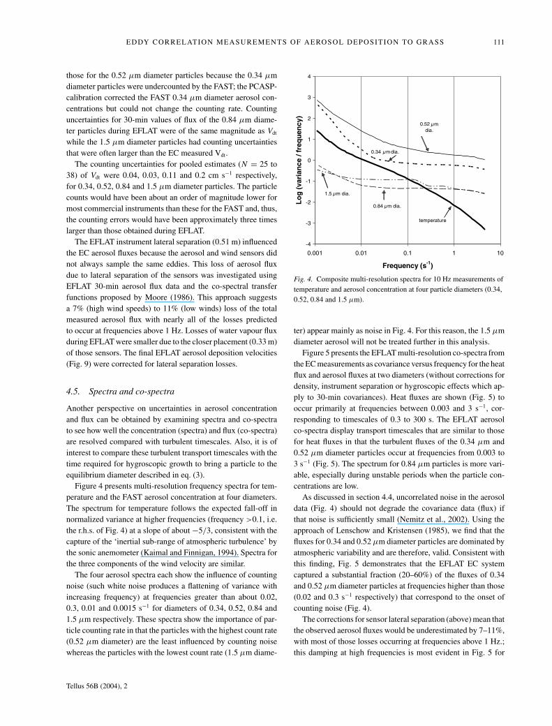
Figure 4 presents multi-resolution frequency spectra for tem-perature and the FAST aerosol concentration at four diameters.The spectrum for temperature follows the expected fall-off innormalized variance at higher frequencies (frequency >0.1, i.e.the r.h.s. of Fig. 4) at a slope of about −5/3, consistent with thecapture of the ‘inertial sub-range of atmospheric turbulence’ bythe sonic anemometer (Kaimal and Finnigan, 1994). Spectra forthe three components of the wind velocity are similar.

The four aerosol spectra each show the influence of countingnoise (such white noise produces a flattening of variance withincreasing frequency) at frequencies greater than about 0.02,0.3, 0.01 and 0.0015 s−1 for diameters of 0.34, 0.52, 0.84 and1.5 µm respectively. These spectra show the importance of par-ticle counting rate in that the particles with the highest count rate(0.52 µm diameter) are the least influenced by counting noisewhereas the particles with the lowest count rate (1.5 µm diame-

-4

-3

-2

-1

0

1

2

3

4

0.001 0.01 0.1 1 10

Frequency (s-1)

Lo

g (

vari

ance

/ fr

equ

ency

)

0.34 m dia.

0.52 dia.

0.84 dia.

1.5 dia.

temperature

m

m

m

Fig. 4. Composite multi-resolution spectra for 10 Hz measurements oftemperature and aerosol concentration at four particle diameters (0.34,0.52, 0.84 and 1.5 µm).

ter) appear mainly as noise in Fig. 4. For this reason, the 1.5 µmdiameter aerosol will not be treated further in this analysis.

Figure 5 presents the EFLAT multi-resolution co-spectra fromthe EC measurements as covariance versus frequency for the heatflux and aerosol fluxes at two diameters (without corrections fordensity, instrument separation or hygroscopic effects which ap-ply to 30-min covariances). Heat fluxes are shown (Fig. 5) tooccur primarily at frequencies between 0.003 and 3 s−1, cor-responding to timescales of 0.3 to 300 s. The EFLAT aerosolco-spectra display transport timescales that are similar to thosefor heat fluxes in that the turbulent fluxes of the 0.34 µm and0.52 µm diameter particles occur at frequencies from 0.003 to3 s−1 (Fig. 5). The spectrum for 0.84 µm particles is more vari-able, especially during unstable periods when the particle con-centrations are low.

As discussed in section 4.4, uncorrelated noise in the aerosoldata (Fig. 4) should not degrade the covariance data (flux) ifthat noise is sufficiently small (Nemitz et al., 2002). Using theapproach of Lenschow and Kristensen (1985), we find that thefluxes for 0.34 and 0.52 µm diameter particles are dominated byatmospheric variability and are therefore, valid. Consistent withthis finding, Fig. 5 demonstrates that the EFLAT EC systemcaptured a substantial fraction (20–60%) of the fluxes of 0.34and 0.52 µm diameter particles at frequencies higher than those(0.02 and 0.3 s−1 respectively) that correspond to the onset ofcounting noise (Fig. 4).

The corrections for sensor lateral separation (above) mean thatthe observed aerosol fluxes would be underestimated by 7–11%,with most of those losses occurring at frequencies above 1 Hz.;this damping at high frequencies is most evident in Fig. 5 for

Tellus 56B (2004), 2

112 R. J . VONG ET AL.

-0.004

-0.002

0

0.002

0.004

0.006

0.008

0.01

0.012

0.014

0.001 0.01 0.1 1 10

Frequency (s-1)

Co

vari

ance

(tu

rbu

len

t fl

ux)

Flux 0.34 m dia., unstable Flux 0.52 dia., unstable Heat flux, unstable

Flux 0.34 m m

m

dia., stable Flux 0.52 dia., stable Heat flux, stable

Heat flux, unstable

Heat flux, stable

Aerosol eddy flux (dia=0.52 m), stable

Aerosol eddy flux (dia=0.52 m), unstable

Aerosol eddy flux (dia=0.34 m)

Fig. 5. Co-spectra for heat flux and aerosolfluxes at two particle diameters.

the 0.52 µm diameter particles for unstable conditions (brokencurve). Thus, the lateral separation corrections (not shown) fur-ther increase the contribution of high-frequency eddies to the to-tal aerosol flux compared with the co-spectra displayed in Fig. 5.

The spectra, co-spectra and particle counting uncertaintiessuggest that the best characterized EC aerosol fluxes ought to bethose for 0.52 µm diameter followed by the flux of 0.34 µm di-ameter particles. The fluxes of 0.84 µm diameter particles havegreater counting uncertainties and should be interpreted withcaution. Most of the EFLAT aerosol turbulent flux occurred attimescales of about 1 to 100 s.

4.6. Aerosol chemical composition and hygroscopicgrowth parameter

Table 1 presents mean values and ranges for the aerosol chemicalcomposition measured over 2- to 3-day periods during EFLAT,

Table 1. Measured aerosol chemical composition (diameter <2.5 µm)

Mean (µg m−3) Mass ratio to UncertaintyAerosol species Concentration Range (µg m−3) (NH4 + SO4) (�pair/mean)

SO4 7.0 1.–18. 0.5–0.7 0.13NH4 4.7 0.6–8. 0.3–0.5 0.15Na 1.4 0.2–3. 0.05–0.25 0.27Ca 0.1 0.05–0.3 0.01–0.03 0.17Elemental carbon 0.06 0–0.12 0–0.02 N.A.Organic carbon 4.0 1.–10. 0.2–0.4∗ N.A.NO3 N.A. N.A. 0.1–0.4∗∗ N.A.

∗Based on the assumed molecular weight of carbon; total organic carbon will be larger.∗∗NO3/(NH4 + SO4) ratio is from a nearby site using the same protocol (Ko, 1992).

the mass ratios of each species to the sum (NH4 + SO4), andthe average uncertainty in concentration (from duplicate filtercollection). These data suggest that the aerosol consisted pri-marily of ammonium bisulfate and organic carbon compounds,with contributions from nitrate and sea salt. Very little elemental(‘black’) carbon was present in the air sampled during EFLAT.

Values for the aerosol hygroscopic growth factor, γ (derivedby fitting eq. (3) to the data of Tang and Mucklewitz (1994), upto an RH of 96%), are presented in Table 2 as a function of solutecomposition and aerosol soluble volume fraction. These growthfactors are valid for the aerosol size range of 0.2 to 1.0 µm.

Given an aerosol chemical composition that is dominated byNH4, SO4, NO3 and organic carbon, the aerosol hygroscopicgrowth parameter, γ , should lie between values of 0.226 and0.261 during EFLAT. The NH4 to SO4 ratio suggests a composi-tion similar to ammonium bisulfate (increasing γ ). The expectedNO3 content also supports a larger value for γ . The lack of

Tellus 56B (2004), 2

EDDY CORRELATION MEASUREMENTS OF AEROSOL DEPOSITION TO GRASS 113

Table 2. Calculated hygroscopic growth parameter, γ

Aerosol composition: ε = 1.0 ε = 0.91 ε = 0.83

(NH4)2 SO4 0.244 0.235 0.226NH4NO3 0.261 0 250 0.241NH4 HSO4 0.261 0.250 0.241

ε = Aerosol volume fraction of the stated chemical composition(soluble fraction). The remaining aerosol volume is assumed to consistof a hygrophobic core (such as soot) that is “internally mixed”.

speciation for the organic aerosol component is the major un-certainty in chemical composition pertaining to hygroscopicgrowth. Some of the organic carbon may be hygrophobic (de-creasing γ ) but the absence of elemental carbon (soot) suggeststhat the EFLAT aerosol was very hygroscopic. Subsequently,we use γ = 0.25 as a “best” value for calculations of the correc-tion to the assembly average aerosol deposition velocity due tohygroscopic growth.

The variability in chemical-mass ratio rather than absoluteconcentration will affect our estimate of hygroscopic growth.The variability in the ratios is much smaller than the variabilityin concentration (Table 1). As a result of uncertainty in aerosolchemical composition we have used a range of growth factorsto estimate the uncertainty in the hygroscopic growth correctionto deposition velocity; the range used for γ was 0.23 to 0.255based on the above chemical and model data and the results ofSwietlicki et al. (2000). Over short (several hours) time peri-ods the mass ratio may have been more variable than shown inTable 1. However, these periods are associated with time changesin aerosol concentration which have already been filtered fromthe EC data set (section 4.2). Thus, the range in γ stated aboveis appropriate for the calculation of the uncertainty in aerosoldeposition velocity associated with hygroscopic growth.

Dry, crystalline particles will grow to 98% of their equilibriumdiameter (diameter at 98% RH) over timescales of 65, 163 and400 ms for particle diameters of 0.25, 0.4 and 0.63 µm respec-tively (Keith and Arons, 1954). During EFLAT the maximumshort-term variation in ambient relative humidity at the EC mea-surement height was no more than 5–7% such that the timescalefor hygroscopic growth (tens of milliseconds) was much lessthan the timescale for vertical transport (tens of seconds) by tur-bulent eddies; this supports the use of an equilibrium model forhygroscopic growth of sub-µm diameter particles.

Future EC experiments would benefit from direct measure-ment of the size distribution at multiple humidities or the hygro-scopic growth factor at several sizes and humidities within therange of interest.

4.7. Hygroscopic growth correction to aerosoldeposition velocity

During EFLAT relatively dry air advected over wet and transpir-ing grass setting up a vertical gradient in RH. For a given aerosol

0.1

1

10

100

1000

0.1 1 10

Aerosol diameter ( m)

dN

/ d

log

D (

cm-3

m-1

)

Beta =4

Fig. 6. Aerosol size distribution from EFLAT from three instrumentsfor consecutive 30-min periods from 3–4 p.m. on 8 June 2000. Aconstant slope (β) of 4 is illustrated (β) for comparison only. Separatevalues of β for each diameter (Table 3) were calculated every 30 minfrom measurements for use in the hygroscopic growth correction (eq.(8)).

dry size, the ambient aerosol diameter was smaller in air aloftthan it was for more humid air near the surface. Thus, upward-moving aerosol contained more liquid water than downward-moving aerosol; this extra water in upward moving particlesusually produced an apparent (false) upward flux of aerosol inthe ‘uncorrected’ EC data for all particles sizes.

Figure 6 presents the aerosol number size distribution for con-secutive 30-min periods during the afternoon of 8 June 2000.Multiple aerosol instruments were used to determine the bestvalues for β for each 30-min period; typical values of β are pre-sented in Table 3 for each diameter at which eddy fluxes weredetermined from the FAST. The large abundance of smaller parti-cles (β > 0) that occurred throughout EFLAT is evident in Fig. 6,as is the 30-min variability in number concentration. These localvalues of β provide the best estimate of the number of smallerparticles that can grow into a specific size interval due to in-creases in RH.

The aerosol deposition velocities for the “best characterized”particle size (0.52 µm diameter) are presented in Fig. 7 as the“corrected-measured” Vdt (for values of γ of 0.235, 0.25 and0.255). Figure 7 also presents the EC measurements and the“apparent deposition velocity due to hygroscopic growth” forγ = 0.25, i.e. −�Vdt (as a dashed line). Whereas the measuredvalues for Vdt and the values of −�Vdt were typically positive(upwards), the “corrected-measured” Vdt are negative (down-ward). The hygroscopic growth correction during EFLAT was

Tellus 56B (2004), 2

114 R. J . VONG ET AL.

Table 3. Slope of the aerosol size distribution, β

EC flux, diameter interval Geometric mean(median diameter) diameter used for β Instruments for β Range for β

0.31–0.375 µm (0.34 µm) 0.22, 0.34 µm HSLAS 3.0 to 5.20.375–0.716 µm (0.52 µm) 0.34, 0.54, 0.77 µm LASX, HSLAS 3.3 to 5.50.716–0.98 µm (0.84 µm) 0.54, 0.77, 0.84 µm FAST,LASX,HSLAS 3.2 to 6.00.98–2.3 µm (1.5 µm) 0.82, 1.4, 1.5 µm FAST,LASX 1.1 to 2.7

Fig. 7. Aerosol deposition velocity(diameter = 0.52 µm) is presented for theEC measurements, hygroscopic growthcorrection, Webb correction and fullycorrected values (for γ = 0.235, 0.25 and0.255).

typically between 0.2 and 0.7 cm s−1 (depending on the hourof the day) with an uncertainty of ± 0.03–0.06 cm s−1 due touncertainty in γ associated with chemical composition. EFLATaerosol deposition velocities are not very sensitive (change in�Vdt ≤ 10%) to the choice of the hygroscopic growth parame-ter within the expected range (0.235 ≤ γ ≤ 0.255).

Figure 8 presents the measured values of saturation ratio (S),saturation ratio flux (w′S′), and the slope of the aerosol sizedistribution (β at 0.52 µm diameter) that were used to calculatethe hygroscopic growth correction (�Vdt). During EFLAT, thesaturation ratio flux exhibited large diurnal variations with lowvalues at night but large values during afternoons. Values ofβ derived from each of the three aerosol instruments exhibiteda marked diurnal variation with minimum values at night andmaximum values during the afternoon. Afternoon measurementsof w′S′ during EFLAT fell between previously reported valuestaken for forests located in Canada and Finland (Buzorius et al.,2000; Kowalski, 2001).

The diurnal variations in β and w′S′ during EFLAT meansthat there are relatively more of the smaller particles (β large)available for hygroscopic growth into a given diameter inter-val and that they will experience larger RH increases (w′S′

large) in the afternoon than at night. Thus, the magnitude of thehygroscopic growth correction in the afternoon is large com-pared with values for morning or night-time periods duringEFLAT. The correction to aerosol turbulent flux (�Vdt) most

0

0.2

0.4

0.6

0.8

1

1.2

0 4 8 12 16 20 24

Hour of day

Sat

ura

tio

n r

atio

or

satu

rati

on

rat

io f

lux

(w

'S'

cm s

-1)

2

3

4

5

Slo

pe

of

the

aero

sol s

ize

dis

trib

uti

on

(B

eta)

w'S'

S = RH/100

Beta

Fig. 8. Components of the hygroscopic growth correction duringEFLAT. Hourly averages of measured values of saturation ratio (S),saturation ratio flux (w′S′), and the slope of the aerosol (diameter =0.52 µm) size distribution (β) are shown for the time periods that areused in Fig. 9.

closely tracks the diurnal variation in saturation ratio flux (Figs. 7and 8).

The calculated hygroscopic growth correction for 0.34 and0.84 µm diameter particles was similar to that for 0.52 µm

Tellus 56B (2004), 2

EDDY CORRELATION MEASUREMENTS OF AEROSOL DEPOSITION TO GRASS 115

diameter particles because �Vdt varies between particle sizesonly due to variation in the slope of the size distribution (β).Aerosol chemical composition was not sufficiently size resolvedfrom EFLAT filter measurements to determine different valuesof γ for different particle diameters even though this composi-tion is known to be size dependent. Thus, the size dependenceof γ, �Vdt, and the “measured-corrected” aerosol deposition ve-locities are not as well characterized as are their average val-ues within the accumulation mode diameter interval (0.3–1 µmhere). Other uncertainties in the size dependence of �Vdt resultfrom the fact that 0.84 µm diameter particles are 2.6 times slowerto reach their equilibrium size than are the 0.52 µm diameter par-ticles (∼ d2 dependence of growth rate; Keith and Arons, 1954).Thus, it is possible that eqs. (3) and (8) overestimate hygroscopicgrowth for the largest aerosol (0.84 µm diameter) consideredhere (Zufall et al., 1998) although Fairall (1984) suggests thatthese particles will reach equilibrium with ambient RH duringturbulent transport and mixing.

The Webb, or density, correction to aerosol flux during EFLATis much smaller than the hygroscopic growth correction, reachinga maximum of 0.05 cm s−1 during the afternoon (circles onFig. 7). The major impact of heat and vapour fluxes on aerosoldeposition velocity corrections is through hygroscopic growthrather than the Webb correction.

The deposition velocities in Fig. 7 represent hourly averagedvalues with RH <96% that passed a quality assurance screeningcriterion; they have not been screened for either wind directionor the morning transition period and, therefore, cannot be con-sidered to represent “deposition to the grass surface”. Examplesof data that do not represent surface deposition are (a) the upwardVdt that are typical at 2 a.m. (increasing aerosol concentrationand, probably, maximum advection from pulp mills that are up-wind during that time of day) and (b) the large downward Vdt

that occur around 7 a.m. (start of the morning transition periodwhen boundary layer growth and flux divergence are occurring).Such data are not included in the final EFLAT results (Fig. 9).

4.8. Aerosol deposition velocity as a functionof stability

Figure 9 presents the EFLAT data that best describe aerosoldeposition to the grass surface, i.e. those that are least likely tohave been sampled during periods of vertical flux divergence.Corrected aerosol deposition velocity for three particle sizes aresummarized for a total of 86 30-min measurement periods withthe very best fetch (NW winds) while avoiding the morningtransition period. Given that there are no obvious aerosol sourcesto the NW, this data stratification minimizes any influence ofadvection.

Figure 9 demonstrates the expected relationship (Lamaudet al., 1994) between deposition velocity (Vdt) and stability (asz/L) in that unstable periods display larger downward (more neg-ative) Vdt than do neutral or stable periods during EFLAT. As

-1

-0.8

-0.6

-0.4

-0.2

0

-0.8 -0.6 -0.4 -0.2 0 0.2 0.4 0.6 0.8

z/L (stability)

Aer

oso

l dep

osi

tio

n v

elo

city

Vd

t [

cm s

-1]

unstable

stable

Vdt (dia =0.52 m)

Vdt (dia= 0.34 )

Vdt (dia = 0.84 )nearly neutral

m

m

Fig. 9. Aerosol deposition velocity varies with stability (z/L). Eddycorrelation field data have been corrected for hygroscopic growth (γ =0.25), sensor lateral separation and density (Webb correction). Pooleduncertainties (counting and hygroscopic growth) are indicated for eachparticle diameter.

conditions changed from stable to unstable, the aerosol deposi-tion velocity for 0.52 µm diameter particles increased from 0.16to about 0.44 cm s−1 while Vdt for 0.34 and 0.84 µm diameterparticles increased from 0.2 to 0.6 and 0.7 cm s−1 respectively.The increased deposition velocity with unstable conditions isexpected because turbulent transport through the atmosphericsurface layer increases and surface impaction of transported par-ticles is likely to be more efficient with the higher wind speedsthat occur.

The consideration of counting and hygroscopic growth uncer-tainties together (assuming that these uncertainties are indepen-dent, e.g. Duan et al., 1988) leads to overall (pooled) uncertaintiesin deposition velocity of 0.072, 0.067 and 0.125 cm s−1 for parti-cle diameters of 0.34, 0.52 and 0.84 µm respectively (displayedas errors bars in Fig. 9).

Since the 0.52 µm diameter particles were typical of theaerosol collected for chemical composition, were counted at100% efficiency, had the smallest counting uncertainties andhave short equilibrium times for hygroscopic growth, we con-sider these 0.52 µm diameter values for Vdt to be the most reli-able. Differences in the values for Vdt for 0.34 and 0.84 µm diam-eter particles (Fig. 9) are not significant given the uncertaintiesassociated with hygroscopic growth and counting statistics.

The EFLAT 0.52 µm diameter value of 0.44 cm s−1 for Vdt

during unstable conditions is a little larger than values reportedby Wesely et al. (1983, 1985) while the EFLAT value of 0.3 cms−1 during near-neutral conditions is similar to experimental val-ues reported by Hummelshoj (1994), Gallagher et al. (1997), andNemitz et al. (2002) for particles of this size.

5. Summary and conclusions

Eddy correlation measurements of aerosol fluxes were per-formed with a new high-flow-rate aerosol spectrometer at a site

Tellus 56B (2004), 2

116 R. J . VONG ET AL.

that was ideal for determining deposition during selected timeperiods. The high flow rates of the FAST spectrometer reduceduncertainties in the flux by increasing the number of particlescounted. Data were selected to avoid vertical divergence in theflux due to advection of upwind source emissions and boundarylayer growth.

The FAST measured aerosol size at ambient RH; this pro-duced aerosol turbulent fluxes that were biased “upwards” dueto vertical changes in RH and particle hygroscopic growth. Thiseffect was quantified by an analysis based on separate measure-ments of aerosol composition, aerosol size distribution, RH andsaturation ratio flux and was removed from the EC field mea-surements to produce estimates of the “true value” of aerosoldeposition velocity to the grass surface for three particle sizes.

Other studies of aerosol deposition velocity could also have abias towards upwards fluxes if based on aerosol diameter that ismeasured at, or near, ambient RH. Studies that dry the aerosol(to RH < 30%) before sensing (Gallagher et al., 1997) ought toavoid this bias and any need for a hygroscopic growth correc-tion. The hygroscopic growth correction to the aerosol flux waslarge in this study because the aerosol was composed of very hy-groscopic compounds, the aerosol size distribution was ‘steep’(there were lots of small particles to grow with increasing RH)and the vertical changes in RH were relatively large due to thepresence of wet soils underlying dry air. Future studies mightfocus on improving estimates of the hygroscopic growth factor(γ ) in order to reduce uncertainties in the hygroscopic growthcorrection (�Vdt) related to the presence of organic or hygro-phobic compounds and their size dependence; real-time valuesof γ could be obtained using tandem differential mobility analy-ses (Swietlicki et al., 2000). For the current study, the correcteddeposition velocities for 0.52 µm diameter particles have an es-timated pooled uncertainty of ±0.07 cm s−1 due to chemicalcomposition (choice of γ ) and counting statistics.

For the best characterized particles (0.52 µm diameter) duringEFLAT, the measured and fully corrected aerosol deposition ve-locity to grass was 0.16 cm s−1 during stable conditions, 0.3 cms−1 in near neutral conditions and 0.44 cm s−1 during unstableconditions.

6. Acknowledgments

The authors thank Siddharth Pavithran and Darren O’Connorfor software development, Rondi Robeson and Marcus Appy forfield measurements, Greg Kok for the PCASP-FAST compari-son, and George Pugh for the use of his grass seed field. Thisproject was supported by NSF grant no. 9907765-ATM (Atmo-spheric Chemistry).

7. Appendix A

Using the Swietlicki et al. (2000) hygroscopic growth relation-ship, the dependence of aerosol equilibrium diameter on satura-

tion ratio S, i.e. RH/100, is

dD/dS = Dγ /(1 − S).

If aerosol size and number are measured at ambient RH, anerror occurs in the corresponding aerosol turbulent flux withinthe specified size interval when that flux is measured by EC. Thiserror occurs for two reasons:

(a) more particles typically grow into a size interval (for β >

0) than out of it when the RH increases;.(b) the dry particle diameters that correspond to the limits of

the size interval change with RH because the interval is definedin terms of diameter at ambient RH.

These two effects can be expressed (Fairall, 1984; Kowalski,2001) as:

N ′ = D′(dN /dD + N /D)

where N ′ is the increase in aerosol number concentration spec-tral density (at a given mean diameter) that is associated withhygroscopic growth during vertical transport.

Introducing the Junge power law to relate the number of par-ticles of different diameters one obtains

N ′/N = −β(D′/D).

Combining this with the definition of deposition velocity andthe change in aerosol size at equilibrium for a perturbation (S′)in saturation ratio (D′ = S′ dD/ dS), the change in the aerosoldeposition velocity due to hygroscopic growth is thus

�Vdt = w′N ′/N = −βw′ D′/D = −β(w′S′/D)(dD/dS)

or

�Vdt = −βγw′S′/(1 − S).

References

Anthoni, P. M., Law, B. E., Unsworth, M. H. and Vong, R. J. 2000. Vari-ation in net radiation over heterogeneous surfaces: measurements andsimulation in a juniper-sagebrush ecosystem. Agric. Forest Meteor.102, 275–286.

Birch, M. and Cary, R. 1996. A thermal-optical technique for analysisof aerosol carbon compounds. Aerosol Sci. Technol. 25, 221–241.

Businger, J. A. 1986. Evaluation of the accuracy with which dry depo-sition can be measured with current micrometeorological techniques.J. Climate Appl. Meteorol. 25, 1100–1124.

Buzorius, G., Rannik, U., Makela, J. M., Keronen, P., Vesala, T. andKulmala, M. 2000. Vertical fluxes measured by the eddy correlationmethod and deposition of nucleation mode particles above a Scotspine forest in southern Finland. J. Geophys. Res. 105, 19 905–19 916.

Buzorius, G., Rannik, U., Nilsson, E. D., Vesala, T. and Kulmala, M.2003. Analysis of measurement techniques to determine dry deposi-tion velocities of aerosol particles with diameters less than 100 nm. J.Aerosol Sci. 34, 747–764.

Tellus 56B (2004), 2

EDDY CORRELATION MEASUREMENTS OF AEROSOL DEPOSITION TO GRASS 117

Duan, B., Fairall, C. W. and Thomson, W. 1988. Eddy correlation mea-surements of the dry deposition of particles in the wintertime. J. Appl.Meteorol. 27, 642–652.

Fairall, C. W., 1984. Interpretation of eddy correlation measurementsof particulate deposition and aerosol flux. Atmos. Environ. 18, 1329–1337.

Gallagher, M. W., Beswick, K. M., Duyzer, J., Westrate, H., Choularton,T. W. and Hummelshoj, P. 1997. Measurements of aerosol fluxes toSpeulder Forest using a micrometeorological technique. Atmos. Env-iron. 31, 359–373.

Hummelshoj, P. 1994. Dry deposition of particles and gases, RISO Na-tional Laboratory Report RISO-R-658(EN), RISO National Labora-tory, Roskilde, Denmark.

Junge, C. E. 1963. Air Chemistry and Radioactivity., Vol. 4, AcademicPress, New York, 114–123.

Kaimal, J. C. and Finnigan, J. J. 1994. Atmospheric Boundary LayerFlows: their Structure and Measurement. Oxford University Press,New York, 33–39.

Keith, C. H. and Arons, A. B. 1954. The growth of seasalt aerosol par-ticles by condensation of atmospheric water vapor. J. Meteorol. 11,173–184.

Ko, L.-J. 1992. Factors influencing the atmospheric aerosol compositionat two sites in western Oregon. M.S. Thesis, Oregon State University,USA.

Kowalski, A. S. 2001. Deliquescence induces eddy covariance and es-timable dry deposition errors. Atmos. Environ. 35, 4843–4851.

Kowalski, A. S. and Vong, R. J., 1999. Near-surface fluxes of cloud waterevolve vertically. Q. J. R. Meteorol. Soc. 125, 2663–2684.

Kowalski, A. S., Anthoni, P. M., Vong, R. J., Delany, A. C. and Maclean,G. D. 1997. Deployment and evaluation of a system for ground-basedmeasurement of cloud water turbulent fluxes. J. Atmos. Ocean Technol.14, 468–479.

Lamaud, E., Brunet, Y., Labatut, A., Lopez, A., Fontan, J. and Druilhet,A., 1994. The Landes experiment: biosphere-atmosphere exchangesof ozone and aerosol particles above a pine forest. J. Geophys. Res.99, D8, 16 511–16 521.

Lenschow, D. H. and Kristensen, L. 1985. Uncorrelated noise in turbu-lence measurements. J. Atmos. Ocean Technol. 2, 68–81.

Moore, C. J., 1986. Frequency response corrections for eddy correlationsystems. Bound. Layer Meteorol. 37, 17–35.

Nemitz, E., Gallagher, M. W., Duyzer, J. H. and Fowler, D. 2002. Mi-crometeorological measurements of particle deposition velocities tomoorland vegetation. Q. J. R. Meteorol. Soc. 128, 2281–2300.

Slinn, W. G. N. 1983. A potpourri of deposition and resuspension ques-tions. In: Precipitation Scavenging, Dry Deposition, and Resuspen-sion, Volume 2, (eds Pruppacher, H. R., Semonin, R. G. and Slinn, W.G. N.) Elsevier Scientific, New York, 1361–1416.

Stull, R. B. 1988. An introduction to boundary layer meteorology. KluwerAcademic, Dordrecht, 90–92.

Swietlicki, E., Zhou, J. Covert, D. S., Hameri, K., Busch, B. and coau-thors, 2000. Hygroscopic properties of aerosol particles in the north-eastern Atlantic during ACE-2. Tellus 52B, 201–227.

Tang, I. N. and Mucklewitz, H. R., 1994. Water activities, densities, andrefractive indices of aqueous sulfates and sodium nitrate droplets ofatmospheric importance. J. Geophys. Res., 99 D9, 18 801–18 808.

Vickers, D. and Mahrt, L. 1997. Quality control and flux sampling prob-lems for tower and aircraft data J. Atmos. Ocean. Technol. 14, 512–526.

Vickers, D. and Mahrt, L. 2003. The cospectral gap and turbulent fluxcalculations. J. Atmos. Ocean. Technol., 20, 660–672.

Vincent, J. H. 1989. Aerosol Sampling, Science and Practice, John Wiley,New York, 86–118.

Vong, R. J. and Kowalski, A. S., 1995. Eddy correlation measurementsof size-dependent cloud droplet turbulent fluxes to complex terrain,Tellus 47B, 331–352.

Webb, E. K., Pearman, G. I. and Leuning, R. 1980. Correction of fluxmeasurements for density effects due to heat and water vapor transfer.Q. J. R. Meteorol. Soc. 106, 85–100.

Wesely, M. L., Cook, D. R. and Hart, R. L. 1983. Fluxes of gases and par-ticles above a deciduous forest in wintertime. Bound. Layer Meteorol.27, 237–255.

Wesely, M. L., Cook, D. R. and Hart, R. L. 1985. Measurements andparameterization of particulate sulfur dry deposition over grass. J.Geophys. Res. 90, 2131–2143.

Zufall, M. J., Bergin, M. H. and Davidson, C. I. 1998. Effects of non-equilibrium growth of ammonium sulfate on dry deposition to watersurfaces. Environ. Sci. Technol. 32, 584–590.

Tellus 56B (2004), 2