Effect of near‐bed turbulence on chronic detachment of epilithicbiofilm: Experimental and modeling approaches

Myriam Graba,1,2 Frédéric Y. Moulin,3 Stéphanie Boulêtreau,1 Frédéric Garabétian,4

Ahmed Kettab,2 Olivier Eiff,3 José Miguel Sánchez‐Pérez,1 and Sabine Sauvage1

Received 24 September 2009; revised 23 June 2010; accepted 6 July 2010; published 20 November 2010.

[1] The biomass dynamics of epilithic biofilm, a collective term for a complexmicroorganism community that grows on gravel bed rivers, was investigated by couplingexperimental and numerical approaches focusing on epilithic biofilm‐flow interactions.The experiment was conducted during 65 days in an artificial rough open‐channel flow,where filtered river water circulated at a constant discharge. To characterize the effectof near‐bed turbulence on the chronic detachment process in the dynamics of epilithicbiofilm, local hydrodynamic conditions were measured by laser Doppler anemometry andturbulent boundary layer parameters inferred from double‐averaged quantities. Numericalsimulations of the EB biomass dynamics were performed using three different modelsof chronic detachment based upon three different descriptors for the flow conditions:Discharge Q, friction velocity u*, and roughness Reynolds number k+. Comparisons ofnumerical simulation results with experimental data revealed chronic detachment to bebetter simulated by taking the roughness Reynolds number as the external physicalvariable forcing chronic detachment. Indeed, the loss of epilithic matter through thechronic detachment process is related not only to hydrodynamic conditions, but also tochange in bottom roughness. This suggests that changes in the behavior and dimensions ofriver bed roughness must be considered when checking the dynamics of epilithic biofilm inrunning waters.

Citation: Graba, M., F. Y. Moulin, S. Boulêtreau, F. Garabétian, A. Kettab, O. Eiff, J. M. Sánchez‐Pérez, and S. Sauvage(2010), Effect of near‐bed turbulence on chronic detachment of epilithic biofilm: Experimental and modeling approaches, WaterResour. Res., 46, W11531, doi:10.1029/2009WR008679.

1. Introduction

[2] “Epilithic biofilm” is a collective term for a complexmicroorganism community that grows on gravel, cobbles,and rocks in river beds and includes algae, bacteria, andmicrofauna, with algae usually the dominant component.This community plays a major role in fluvial ecosystemsbecause it is the source ofmost primary production [Minshall,1978; Lock et al., 1984], and constitutes a food source for anumber of invertebrates and fish [Fuller et al., 1986; Mayerand Likens, 1987; Winterbourn, 1990]. It also plays a majorrole in the metabolic conversion and partial removal of bio-degradable material in rivers and streams [McIntire, 1973;Saravia et al., 1998; Hondzo and Wang, 2002]. Thus, forbetter management of fluvial ecosystems dominated by fixedbiomass in the near‐bed region, epilithic biofilm dynamics

should be considered in numerical modeling of biogeo-chemical transfer.[3] A large number of models have been designed to

describe the biomass dynamics of the epilithic biofilm.Some complex models focus on different component speciesof the epilithic biofilm [e.g., Asaeda and Hong Son, 2000,2001; Flipo et al., 2004], whereas simpler models [e.g.,McIntire, 1973; Horner and Welch, 1981; Horner et al.,1983; Momo, 1995; Uehlinger et al., 1996; Saravia et al.,1998] relate the peak biomass of epilithic biofilm to envi-ronmental variables such as nutrient concentration, lightintensity, and flow discharge. The main processes involvedin these models can be summarized in dB/dt = C + G − D,where B is the biomass, C the colonization function, G thegrowth function, and D the detachment function, which candescribe chronic, autogenic, or catastrophic detachment, or acombination of these. These models have been developedeither to explain processes observed in natural streams andrivers [Uehlinger et al., 1996; Saravia et al., 1998] or inartificial channels and laboratory streams [McIntire, 1973]. Insome cases, the processes of colonization and growth are notmodeled separately [Horner and Welch, 1981; Horner et al.,1983] or the detachment process is ignored [Momo, 1995].[4] Among these models, that of Uehlinger et al. [1996]

has been most frequently used for natural or artificial riverflows [Fothi, 2003; Boulêtreau et al., 2006, 2008; Labiodet al., 2007]. In fact, although this model has been applied

1ECOLAB, Universite de Toulouse, UPS, INPT, CNRS, Toulouse,France.

2Laboratoire des Sciences de l’Eau, Ecole Nationale Polytechnique,Algiers, Algeria.

3IMFT, Universite de Toulouse, UPS, INPT, ENSEEIHT, CNRS,Toulouse, France.

4UMR 5805, Station Marine d’Arcachon, EPOC-OASU, UniversiteBordeaux 1, Arcachon, France.

Copyright 2010 by the American Geophysical Union.0043‐1397/10/2009WR008679

WATER RESOURCES RESEARCH, VOL. 46, W11531, doi:10.1029/2009WR008679, 2010

W11531 1 of 15

successfully to reproduce the temporal variations in epilithicbiofilm biomass in natural rivers (Swiss pre‐alpine gravelbed river systems) [Uehlinger et al., 1996], it had beendeveloped earlier by McIntire [1973] through experimentsin laboratory open‐channel flows. This model was recentlyapplied byBoulêtreau et al. [2006] to the large Garonne Riverusing an additional term to include autogenic detachment.The level of complexity of this model was also investigatedby using the Akaike Information Criterion (AIC) to determinethe minimum adequate parameter set required to describe thebiomass dynamics. Boulêtreau et al. [2006] found that in 9 ofthe 11 cases studied, the best model was one that described anequilibrium between phototrophic growth and discharge‐dependent chronic loss, and that ignored light, temperature,nutrient influences, and catastrophic and/or autogenicdetachment terms. This simplified model is

dB

dt¼ G� D ¼ �maxB|fflffl{zfflffl}

G1

1

1þ kinvB|fflfflfflfflffl{zfflfflfflfflffl}G2

�CdetQ B|fflfflfflffl{zfflfflfflffl}D

; ð1Þ

where B (g m−2) is the epilithic biofilm biomass, t (days) is thetime, mmax (d

−1) is the maximum specific growth rate at thereference temperature 20°C, kinv (g

−1 m2) is the inverse half‐saturation constant for biomass, Cdet (s m−3 d−1) is anempirical detachment coefficient, and Q (m3 s−1) is the flowdischarge. In this simplified model, G is a growth functionformed by the linear term G1, which describes the expo-nential increase in biomass, and the termG2, which describesthe effect of density limitation and characterizes the biomasslimitation of the growth rate. It accounts for the phenomenonof biomass growth rate decreasing with increasing epilithicbiofilm mat thickness, due to limitations in light and nutrientconcentration in the inner layers of the biofilm. Term D is thedetachment function, which is controlled here by Q and B,and does not take into account grazing or catastrophic loss ofbiomass due to bed movement. These two latter processeswere assumed negligible or nonexistent in our laboratoryexperiments.[5] Several previous studies have investigated the mutual

influences of epilithic biofilm and stream flow. Early studiesfocusing on the effect of current on epilithic biofilm accrualshowed that there is intraspecific competition in the epilithicbiofilm assemblage, mainly driven by current velocity [Ghoshand Gaur, 1998]. Some authors [e.g., Horner and Welch,1981; Stevenson, 1983] observed a positive correlation,with biomass increasing in proportion to increasing velocity,whereas others [Ghosh and Gaur, 1998] found an inverserelationship between epilithic accumulation and currentvelocity.[6] At present, it is generally recognized that flow is an

important factor involved directly or indirectly in manyrelevant processes (e.g., colonization, metabolism, nutrientfluxes, and detachment) of epilithic biofilm dynamics[Stevenson, 1983; Reiter, 1986; Uehlinger et al., 1996;Saravia et al., 1998; Hondzo and Wang, 2002; Boulêtreauet al., 2006, 2008]. Retroactively, its presence and its ageare important factors that modify local hydrodynamic char-acteristics such as the equivalent roughness height ks and thefriction velocity u*. Reiter [1989a, 1989b] and Nikora et al.[1997, 1998] found that u*, which measures the drag of theflow at the bottom, increased with the growth of the epilithicbiofilm, leading to the conclusion that epilithic biofilm

increased bed roughness. In contrast, Biggs and Hickey[1994] observed that epilithic biofilm decreased the rough-ness of the substratum.[7] These early studies demonstrated the complexity of

flow‐epilithic biofilm interactions and have motivated fur-ther research in the past decade [Godillot et al., 2001;Nikora et al., 2002; Hondzo and Wang, 2002; Fothi, 2003;Labiod et al., 2007; Moulin et al., 2008a]. The latter studiesshow that the presence of the epilithic biofilm induces aclear variation in turbulence intensity and Reynolds stress inthe benthic zone. Moulin et al. [2008a] showed how dif-ferent hydrodynamic conditions promote different growthpatterns of epilithic biofilm (dense mat or porous mat withlong filaments) and yield different values of the equivalentroughness height ks, even for approximately the sameamount of biomass.[8] The interfacial region between the epilithic biofilm

and the flow plays a major role, and its description requireslocal parameters associated with the turbulent processesinstead of vertically integrated quantities such as flow dis-charge or mean longitudinal velocity (as used in the detach-ment term byHorner andWelch [1981],Horner et al. [1983],and Saravia et al. [1998]). Thus, Fothi [2003] suggested re-placing the flow discharge Q with the roughness Reynoldsnumber k+ = u* ks/n (where n is water kinetic viscosity and ksthe equivalent roughness height) in the detachment term ofthe model by Uehlinger et al. [1996]. However, Labiod et al.[2007] adopted an intermediate step by taking the frictionvelocity u* as an external physical parameter for the detach-ment. First evaluations of these models [Fothi, 2003; Labiodet al., 2007] with laboratory experiments in open‐channelflows gave better results than the early model of Uehlingeret al. [1996]. However, additional experimental data arerequired to determine the relevance of u* or k+ alone todescribe the chronic detachment term. The main objectiveof the present study was to test and compare these twoequations of the chronic detachment term through furtherexperiments and to help answer the central question thatstream biologists ask their physics colleagues [see Hart andFinelli, 1999], i.e., “What flow parameters should be mea-sured to obtain the most appropriate quantification of thephysical environment for stream biota?” when discussing theepilithic biofilm chronic detachment process.

2. Theoretical Background

2.1. Spatial Averaged Flow and Log Law Formulation

[9] It should be noted that our experiment was conductedin steady, uniform, open channel flow, over a rough bedwith a high relative submergence (flow depth H � rough-ness height D). In such free surface turbulent boundarylayers, it is possible to distinguish three principal layers [see,e.g., Nikora et al., 2001, 2007a, 2007b]: (1) An outer layer(z > 0.2 H), (2) a logarithmic layer that occupies the flowregion (2–5) D < z < 0.2 H, and (3) a roughness layer com-posed of a form‐induced sublayer in the region just abovethe roughness crests D < z < (2–5) D and an interfacialsublayer (or canopy) that occupies the flow region belowthe crests z < D.[10] Recently, Lopez and Garcia [1998, 2001] and Nikora

et al. [2002] demonstrated experimentally and theoreticallythat in such flows over a rough bottom, double‐averagedquantities (i.e., quantities averaged in time and in the two

GRABA ET AL.: EPILITHIC BIOFILM AND ROUGH FLOW INTERACTION W11531W11531

2 of 15

horizontal directions x and y and denoted hixy) lead to a betterdescription of the roughness sublayer. Double‐averagingyields, for instance a quasi‐linear velocity profile deep insidethe roughness sublayer in the interfacial sublayer, extends thevalidity range of the log law towards the top of the roughnessin the form‐induced sublayer; thus, leading to more robustestimations of the boundary layer parameters u*, z0, and d[McLean and Nikora, 2006; Nikora et al., 2007a, 2007b;Moulin et al., 2008a], which appear in the generalized log lawformula

hUixyu*

¼ 1

�ln

z� d

ks

� �þ A ¼ 1

�ln

z� d

z0

� �; ð2Þ

where � is the Von Karman constant (� ≈ 0.4), u* the frictionvelocity, z the distance from the flume bed, d the displace-ment length (also known as a zero‐plane displacement) andz0 = ks exp(−� A) the roughness length, and A being a constantthat depends on flow regime (A ≈ 8.5 for fully rough flows,i.e., k+ > 70 [see, e.g., Nezu and Nakagawa, 1993]).

2.2. Chronic Detachment Function Formulation

[11] As underlined previously, the detachment equationwith a global hydrodynamic parameterQ (m3 s−1) [Uehlingeret al., 1996] cannot realistically describe a phenomenon suchas the detachment that occurs on the bed where epilithicbiofilm grows. However, the function of detachment can bedescribed in a more pertinent equation by taking as externalphysical variables local hydrodynamic characteristics, suchas friction velocity u* [Labiod et al., 2007] or the roughnessReynolds number k+ (k+ = u* ks/n) [Fothi, 2003].[12] Thus, three models can be inferred from equation (1),

with three formulations for the chronic detachment functionDas

D ¼ d1 ¼ CdetQ B; ð3Þ

D ¼ d2 ¼ Cdet0 u*B; ð4Þ

D ¼ d3 ¼ Cdet00 kþB; ð5Þ

where Q (m3 s−1) is the discharge flow, u* (m s−1) the frictionvelocity, (k+= u* ks/n) the dimensionless roughness Reynolds

number, and Cdet (s m−3 d−1), Cdet

′ (s m−1 d−1), and Cdet′′ (d−1)

the detachment coefficients.

3. Materials and Methods

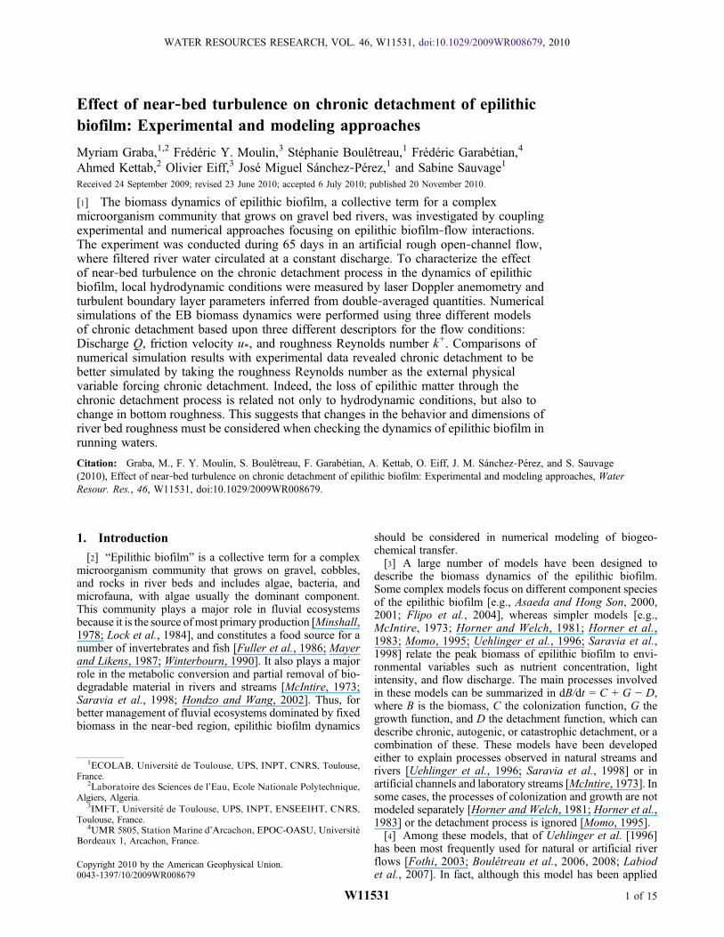
3.1. Experimental Design and Procedure

[13] The experiment was performed in the indoor exper-imental flume used by Godillot et al. [2001] and Labiodet al. [2007], located at the Institute of Fluid Mechanics,Toulouse, France. The flume is 11 m long, 50 cm wide, and20 cm deep, with Plexiglas sides (10 mm thick) and a PVCbase (20 mm thick). The bed slope is 10−3 and the hydrauliccircuit is a closed loop. For the present study, this experi-mental flume was modified to run using a partial recircu-lation system, thereby allowing the use of Garonne Riverwater with no nutrient limitation, but with complete controlof the hydrodynamic conditions. The partial recirculationsystem (Figure 1) consists of an initial pump (Selfinox200/80T, ITT Flygt) that continuously supplies water fromthe river to the outlet reservoir (3300 L) with a flow dis-charge of 800 L h−1 (ensuring a complete turnover of waterin the system every 4 h), and a second submerged pump(Omega 10‐160‐4, Smedegard) that supplies water to theinlet reservoir (1500 L). The water flows by gravity throughthe experimental flume from the inlet reservoir to the outletreservoir. Convergent and guiding grids are placed in theinlet reservoir to ensure quasi‐uniform entry flow. Amoderate current velocity (0.22 m s−1) was selected in thepresent study to enhance microorganism colonization andgrowth [Stevenson, 1983].[14] The Garonne River water was treated to reduce the

supply of suspended matter and to exclude grazers; largeparticles were eliminated by two centrifugal separators, andthe water was then filtered 3 times through filters with 90,20, and 10 mm pores. Light was supplied by six 1.5 m longracks of five evenly distributed neon tubes (“daylight”,Philips TLD 58 W) and fluorescent tubes (Sylvania Gro‐Lux 58 W; designed for enhancing photosynthesis as theyemit in the visible red area). Photoperiod was set at 16 hoursof day and 8 hours of night. The incident light, measuredwith an LI‐190SA quantum sensor and an LI‐1000 datalogger (LI‐COR), varied between 140 and 180 mmol m−2 s−1

photosynthetically active radiation (PAR) on the channelbottom, ensuring photosynthetic activity saturation [Bothwellet al., 1993].

Figure 1. Longitudinal view of the experimental flume.

GRABA ET AL.: EPILITHIC BIOFILM AND ROUGH FLOW INTERACTION W11531W11531

3 of 15

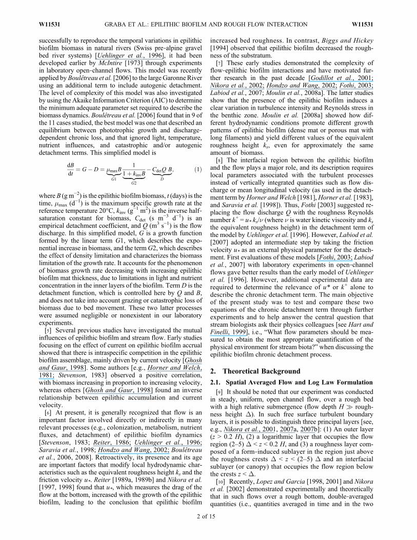
[15] The bottom of the flume is completely covered byartificial cobbles that mimic natural cobbles (see Figure 2).Each artificial cobble consists of a chemically inert sand‐ballasted polyurethane resin hemisphere (37 mm diameter,20 mm high), with a shape and texture shown to providegood conditions for epilithic biofilm adhesion and growth[Nielsen et al., 1984] and with a resistance to temperature of110°C. To eliminate any possible toxicity due to artificialcobble manufacture (e.g., solvents), cobbles were immersedin river water for 3 weeks, then washed with tap water andsterilized by autoclave (120°C, 20 min) before being posi-tioned side by side in the flume. The artificial cobbles arenot fixed in place so that they could be sampled.[16] To obtain diverse epilithic biofilm communities,

pebbles (average size 10 cm2) with biofilm were collected insouthwest France streams (Ariège (09) and Gave de Pau (05))and rivers (Garonne (7) and Tarn (8)) displaying a wide rangeof hydroecological conditions. These pebbles were stored inanother running flume that was dedicated to providing bio-film matter for our experiment. A biofilm suspension wasproduced by scraping the upper surface of 15 randomlyselected pebbles with a toothbrush, and adding the obtainedproduct to 1 L of filtered (0.22 mm pore size) water. Thebiofilm suspension was crushed, then homogenized (tissuehomogenizer) to remove macrofauna and approach a grazer‐free condition. For 3 weeks, the flume was run using closedrecirculation; that is, the water was renewed weekly, and justafter renewal, it was seeded with the prepared biofilm sus-pension. After the seeding (inoculum) stage, the closed cir-culation flume was changed to an open circulation flumeto allow free growth of epilithic biofilm on the bed inwater without nutrient limitation. During the epilithic biofilmgrowth experiment (65 days), which comprised severalstages, hydrodynamic and biological measurements wereperformed and upper view photographs of the artificial cob-bles were taken daily through a Plexiglas window located atthe water surface (Nikon camera with 194 2000 × 1312 pixelresolution).

3.2. Biological Sampling and Measurements

3.2.1. Epilithic and Drift Biomass[17] After the seeding phase, biofilm biomass was sam-

pled every week randomly along a 5 m length in the center

of the experimental flume (see Figure 1). The three rows ofcobbles closest to the walls of the flume were not sampled toavoid edge effects. To minimize the errors of measurementwithout disrupting the experiment, 10 cobbles were extractedon each sampling occasion and kept in sterile vials at 4°C.Subsequently, six were used to measure Ash Free Dry Mass(AFDM) and four to measure chlorophyll‐a (Chl‐a) massby developed surface. Every cobble sampled was replacedwith a new pink‐colored one, to avoid resampling. Cobblesused for AFDM determination were dried (80°C, overnight),weighed (W1), and scraped. Cobbles were then cleaned andweighed (W2) to obtain Dry Mass (DM) by differencebetween W1 and W2. One portion (around 25 mg) of scrapeddry matter was weighed before and after combustion (500°C,overnight) to determine AFDM.[18] For Chl‐a mass determination, biofilm was scraped

from the upper surface of the four other cobbles with asterile toothbrush, and suspended in filtered (0.2 mm,Whatman cellulose nitrate membrane) water (50 or 100 mLaccording to biomass). Suspensions were homogenized (tissuehomogenizer) and a 10mL aliquot was centrifuged (12000 × g,20 min, 4°C). After removing the supernatant, the pellet wasstored at −80°C, and Chl‐a was measured spectrophotomet-rically using trichromatic equations [Jeffrey et al., 1997] afterextraction with 90% acetone (4 hours, darkness, room tem-perature) of the suspended (tissue homogenizer) and ground(ultrasonic disintegrator) pellets.3.2.2. Algal Composition[19] Biofilm was removed from the upper surface of one

cobble with a sterile toothbrush and suspended in filtered(0.2 mm) water (50 mL) for algal composition. The biofilmsuspension was preserved with glutaraldehyde (1% finalconcentration) and stored refrigerated in darkness untilexamination at 600 to 1000 X. Taxa were identified to thelowest practical taxonomic level; usually to species, butoften to genus. For practical reasons, five of seven sampleswere selected for analysis to observe changes in taxonomiccomposition.

3.3. Hydrodynamic Measurements

[20] Water discharge was controlled by a sluice gate and abypass, and measured by an electromagnetic flow meterplaced in the return pipe of the flume. The water depth wasmeasured with a millimeter scale.[21] To estimate double‐averaged quantities with a Laser

Doppler Anemometer (LDA), the velocity components weremeasured at the centerline of the flume and in a sectionequipped with glass windows located 8 m from the flumeentrance (Figure 1). The measurement points were situatedat heights varying from 20 to 120 mm from the bottom (with2 mm space intervals between z = 20 and 50 mm, and 10 mmintervals up to z =120 mm) along three contrasting verticalprofiles A, B, and C (Figure 2). The bottom (z = 0) corre-sponds to the level of the bed flume without hemispheres. ASpectra‐Physics bi‐composant Argon Laser equipped with a55L modular optic Disa and with wavelengths of 514.5 nm(green ray) and 488 nm (blue ray) was used. This device wasplaced on a support that was fixed in the longitudinal direc-tion but that allowed horizontal and vertical movement.Signal acquisition was obtained with a photomultiplicatorplaced in the broadcast lamp and recovered by a BurstSpectrum Analyzer (BSA), which processed the Doppler

Figure 2. (a) Positions of the vertical profiles A, B, and C forLDA measurements and double‐averaging (<Values>xy =(2 Values in A + 4 Values in B + 2 Values in C)/8 = (Valuesin A + 2 Values in B + Values in C)/4). (b) Photograph of anartificial cobble.

GRABA ET AL.: EPILITHIC BIOFILM AND ROUGH FLOW INTERACTION W11531W11531

4 of 15

signal and calculated the Doppler frequency and then theinstantaneous velocities. The data obtained were then pro-cessed and stored in a computer with Dantec Burstware 2.00software.[22] For each measurement point, data acquisition was

performed during 4 minutes of n LDA observations (n = 104

to 1.5 × 104) with instantaneous longitudinal U, transverseV, and vertical W velocity components, from which time‐averaged velocity components U , V , root‐mean‐square(RMS) values of the turbulent fluctuations u′, v′, and w′, andthe mean turbulent shear stress u0w0 were inferred. Observa-tions of n = 104 yielded good estimation of the averagedvelocities, but n = 1.5 × 104 acquisitions were necessary forconvergence of the mean turbulent shear stress. The double‐averaged turbulent shear stress hu0w0ixy and longitudinalvelocity hUixy profiles were obtained by space‐averagingwith respective weight factors of 1, 2, and 1 for the mea-surements in the three vertical profiles A, B, and C, respec-tively (see Figure 2), in accordance with the influential areaof the three profiles. At the beginning of the experiment,measurements of the vertical velocity W were not availablebecause of a malfunction of the W laser beam.[23] To infer the friction velocity u* from the turbulent

quantities, we followed Cheng and Castro [2002] when thedouble‐averaged turbulent shear stress hu0w0ixy was avail-able, using

u* ¼ limz!d

ffiffiffiffiffiffiffiffiffiffiffiffiffiffiffiffiffiffiffihu0w0i2 xy

q: ð6Þ

When the double‐averaged turbulent shear stress was notavailable, we followed Labiod et al. [2007] and used the

values of the space averaged urms =ffiffiffiffiffiffiu02

pto fit in the

exponential profiles of Nezu and Nakagawa [1993]:ffiffiffiffiffiffiu02

pu*

¼ Du exp �Ckz

H � d

� �; ð7Þ

whereCk andDu are empirical constants (Ck = 1 andDu = 2.3).[24] The double‐averaged velocity profiles hUixy were

then fitted with the log law to determine z0 and d bychoosing the best values inferred from a linear regression ofexp(� hUixy/u*) = (z − d)/z0 in the region between the top ofthe cobbles at z = D and the top of the logarithmic layertaken as z = 0.2 H [Wilcock, 1996], followed by a nonlinearbest fit of � hUixy/u* = log (z‐d) − log(z) (to be consistentwith previous works where the log law is generally fittedin the (U, log(z − d)) plane). The equivalent roughnessheight ks established by Nikuradse was inferred from ks =z0 exp(� 8.5), and the roughness Reynolds number k+ fromk+ = u* ks/n [Nezu and Nakagawa, 1993].[25] In the LDA measurements, difficulties were encoun-

tered with the algal filaments, which moved and disturbeddata acquisition. However, the top of the biofilm mat couldthen be defined as the lowest height of validated measure-ments, and was therefore used as the lower limit for the fit-ting of data with the log law.

3.4. Numerical Model Description

[26] We noted that in equation (1), inferred from themodel of Uehlinger et al. [1996], colonization is not con-sidered. We therefore decided to describe the colonization

process by an initial condition for the biomass, adopting anumerical parameterization [Belkhadir et al., 1988;Capdevilleet al., 1988] to determine the value of the initial epilithic bio-mass denoted Binit.[27] According to the considerations above, and while

knowing that the factors of light, temperature, nutrientavailability, and grazers were controlled in our experiment,the differential equation (1) for each of the three detachmentequations (3), (4), and (5) was solved numerically by codingthe fourth‐order Runge‐Kutta method in Fortran 90. Pre-liminary tests demonstrated that a time step fixed at 3 hourswas a good condition to reduce errors caused by numericalintegration. Values of the input data discharge Q, frictionvelocity u*, and roughness Reynolds number k+ at each timestep were obtained by linear interpolation of the experimentaldata. To calibrate the models, we started by setting the valuesof the maximum specific growth mmax (d

−1), the inverse half‐saturation constant kinv (g

−1 m2), and the initial biomass Binit

in the range of values reported in the literature from field,laboratory, and modeling studies for phytoplanktonic andbenthic algae [Auer and Canale, 1982; Borchardt, 1996;Uehlinger et al., 1996; Boulêtreau et al., 2008]. The para-meters Cdet, Cdet

′ , and Cdet′′ were then adjusted to best fit the

simulated values of each of the three detachment equationswith experimental data.[28] Two indices were used to test the performance of the

models and the agreement between measured and simulatedresults and to compare the efficiency of the three modelstested: The c2 of conformity [Uehlinger et al., 1996] givenby

�2 ¼XNi¼1

B tið Þ � Bmeas;i

ESmeas;i

� �2

; ð8Þ

and the Nash‐Sutcliffe coefficient of efficiency E [Lekfiret al., 2006; Kliment et al., 2008] by

E ¼ 1�PNi¼1

Bmeas;i � B tið Þ� 2PNi¼1

Bmeas;i � Bmeas

� 2 ; ð9Þ

where Bmeas,i is the measured biomass, B(ti) the predictedbiomass at time i,ESmeas,i is the standard error inBmeas, i,Bmeas

is the average of all measured values, and N is the number ofmeasurements. Generally the model is deemed perfect whenE is greater than 0.75, satisfactory whenE is between 0.36 and0.75, and unsatisfactory when E is smaller than 0.36 [Krauseet al., 2005].

4. Results and Discussion

4.1. Biomass Dynamics Data and Algal Composition

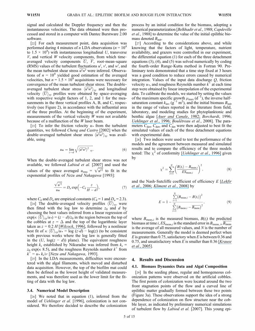
[29] In the seeding phase, regular and homogeneous col-onization patterns were observed on the artificial cobbles.The first points of colonization were located around the twofront stagnation points of the flow and a curved line ofepilithic matter gradually formed between these two points(Figure 3a). These observations support the idea of a strongdependence of colonization on flow structure near the cob-ble layer, as indicated by preliminary numerical simulationsof turbulent flow by Labiod et al. [2007]. This young epi-

GRABA ET AL.: EPILITHIC BIOFILM AND ROUGH FLOW INTERACTION W11531W11531

5 of 15

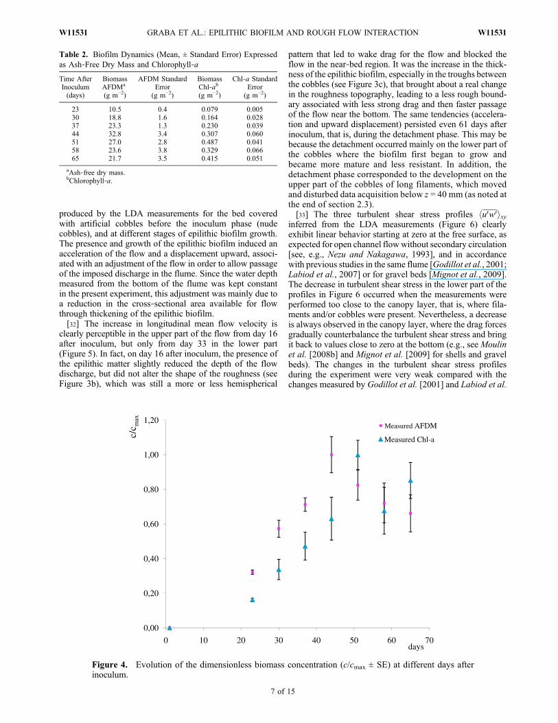
lithic biofilm, in which the diatoms were dominant (seeTable 1), then covered all surfaces exposed to the light fromabove, including the troughs between the cobbles. Themeasured values (g m−2) of AFDM and Chl‐a, with thecorresponding values of the standard errors (SE, g m−2)during the different stages of epilithic biofilm growth, arepresented in Table 2, and are plotted in Figure 4 in terms ofdimensionless numbers (c/cmax). In these, c is the measuredAFDM or Chl‐a and cmax is the maximum reached, which isequal to 32.8 ± 3.4 g m−2 for AFDM and 0.487 ± 0.041 g m−2

for Chl‐a. Thus in the first three weeks, AFDM increased to avalue of 10.5 ± 0.4 g m−2, which represented 32.2 ± 1.23% ofmaximum growth (see Figure 4). The rate of increase thenaccelerated over a further 3 week period and AFDM reached100 ± 10.5% of maximum growth at 44 days after inoculum.There followed a phase of loss, dominated by detachment,leading to a decrease to 66.1 ± 10.7% of maximum growth(21.7 ± 3.5 g m−2) during the next 3 weeks. For Chl‐a, 33.7 ±5.85% (0.164 ± 0.028 g m−2) of the maximum value wasreached on day 30 after inoculum and the peak (100 ± 8.47%)was reached on day 51. The subsequent loss phase caused adecrease to 85.2 ± 10.4%of themaximum (0.415 ± 0.051 gm−2)during the two last weeks.[30] The algal community was dominated by diatoms,

which represented 98–100% of the total abundance. Twotaxa strongly dominated the algal community: Fragilariacapucina represented 46%–64% and Encyonema minutumrepresented 18%–37% of the total community, and the theo-retical transition from diatoms to Chlorophyceae [Stevenson,1996] was not observed, even at the end of the experiment(see Table 1).

4.2. Hydrodynamic and Boundary Layer Parameters

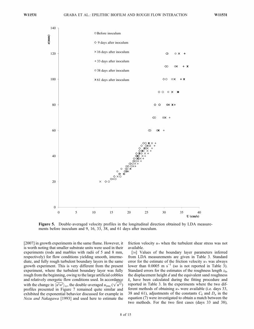
[31] Figure 5 shows the longitudinal velocity U at A, B, Cand the double‐averaged longitudinal velocity hUixy profiles

Figure 3. Biomass dynamics phases during constant discharge (14.4 m3 s−1) in comparison with an ide-alized benthic algal accrual curve [Biggs, 1996]: (a) 7 days after inoculum, (b) 14 days after inoculum,(c) 30 days after inoculum, (d) 52 days after inoculum.

Table 1. Relative Abundance (%) of Diatom Species at DifferentBiofilm Growth Stages

Diatom Species

Time After Inoculum (days)

23 44 51 58 65

Achnanthidium minutissimum (Kütz.)Czarnecki

0 1 0 0 2

Encyonema minutum Hilse ex.Rabenhorst

19 37 25 27 18

Encyonema silesiacum (Bleischin Rabh.) D.G. Mann

1 3 2 0 1

Diatoma vulgaris Bory 1824 5 2 0 13 14Fragilaria capucina Desmazieresvar. vaucheriae (Kütz)Lange‐Bertalot

64 48 55 46 57

Fragilaria crotonensis Kitton 0 0 8 12 0Fragilaria ulna (Nitzsch.)Lange‐Bert. v. oxyrhynchus(Kutz.) Lange‐Bertalot

2 0 0 0 0

Gomphoneis minuta (Stone) Kociolek& Stoermer var. minuta

0 0 1 0 0

Comphonema parvulum (Kützing)Kützing var. parvulum f. parvulum

0 0 1 0 0

Gomphonema sp. 1 0 0 0 0Fragilaria arcus (Ehrenberg)Cleve var. arcus

1 0 0 0 0

Melosira varians Agardh 2 1 2 1 3Navicula tripunctata (O.F. Müller)Bory

1 1 2 0 0

Navicula sp. 1 0 0 0 0Nitzschia acicularis (Kützing)W.M. Smith

1 0 0 0 0

Nitzschia dissipata (Kützing)Grunow var. dissipata

1 3 2 0 1

Nitzschia fonticola Grunow inCleve et Möller

1 3 1 1 2

Nitzschia frustulum (Kützing)Grunow var. frustulum

0 0 0 0 1

Nitzschia palea (Kützing) W. Smith 0 0 0 0 1Nitzschia sp. 0 1 0 0 0Surirella angusta Kützing 0 0 1 0 0

GRABA ET AL.: EPILITHIC BIOFILM AND ROUGH FLOW INTERACTION W11531W11531

6 of 15

produced by the LDA measurements for the bed coveredwith artificial cobbles before the inoculum phase (nudecobbles), and at different stages of epilithic biofilm growth.The presence and growth of the epilithic biofilm induced anacceleration of the flow and a displacement upward, associ-ated with an adjustment of the flow in order to allow passageof the imposed discharge in the flume. Since the water depthmeasured from the bottom of the flume was kept constantin the present experiment, this adjustment was mainly due toa reduction in the cross‐sectional area available for flowthrough thickening of the epilithic biofilm.[32] The increase in longitudinal mean flow velocity is

clearly perceptible in the upper part of the flow from day 16after inoculum, but only from day 33 in the lower part(Figure 5). In fact, on day 16 after inoculum, the presence ofthe epilithic matter slightly reduced the depth of the flowdischarge, but did not alter the shape of the roughness (seeFigure 3b), which was still a more or less hemispherical

pattern that led to wake drag for the flow and blocked theflow in the near‐bed region. It was the increase in the thick-ness of the epilithic biofilm, especially in the troughs betweenthe cobbles (see Figure 3c), that brought about a real changein the roughness topography, leading to a less rough bound-ary associated with less strong drag and then faster passageof the flow near the bottom. The same tendencies (accelera-tion and upward displacement) persisted even 61 days afterinoculum, that is, during the detachment phase. This may bebecause the detachment occurred mainly on the lower part ofthe cobbles where the biofilm first began to grow andbecame more mature and less resistant. In addition, thedetachment phase corresponded to the development on theupper part of the cobbles of long filaments, which movedand disturbed data acquisition below z = 40 mm (as noted atthe end of section 2.3).[33] The three turbulent shear stress profiles hu0w0ixy

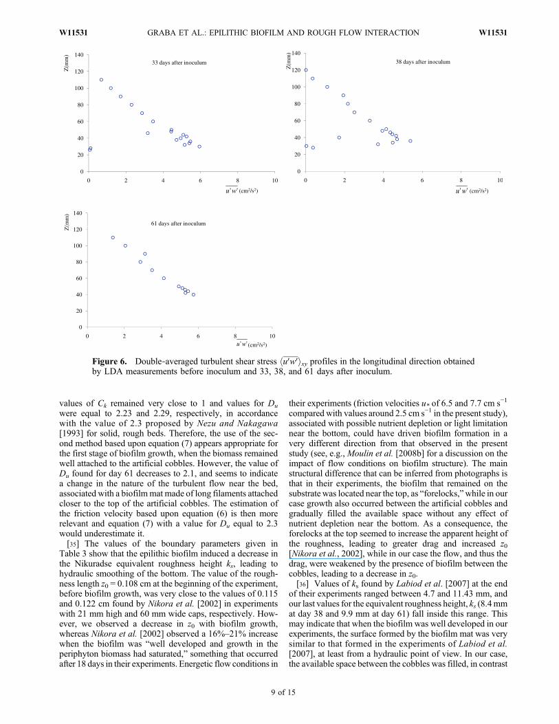
inferred from the LDA measurements (Figure 6) clearlyexhibit linear behavior starting at zero at the free surface, asexpected for open channel flowwithout secondary circulation[see, e.g., Nezu and Nakagawa, 1993], and in accordancewith previous studies in the same flume [Godillot et al., 2001;Labiod et al., 2007] or for gravel beds [Mignot et al., 2009].The decrease in turbulent shear stress in the lower part of theprofiles in Figure 6 occurred when the measurements wereperformed too close to the canopy layer, that is, where fila-ments and/or cobbles were present. Nevertheless, a decreaseis always observed in the canopy layer, where the drag forcesgradually counterbalance the turbulent shear stress and bringit back to values close to zero at the bottom (e.g., see Moulinet al. [2008b] and Mignot et al. [2009] for shells and gravelbeds). The changes in the turbulent shear stress profilesduring the experiment were very weak compared with thechanges measured by Godillot et al. [2001] and Labiod et al.

Table 2. Biofilm Dynamics (Mean, ± Standard Error) Expressedas Ash‐Free Dry Mass and Chlorophyll‐a

Time AfterInoculum(days)

BiomassAFDMa

(g m−2)

AFDM StandardError(g m−2)

BiomassChl‐ab

(g m−2)

Chl‐a StandardError(g m−2)

23 10.5 0.4 0.079 0.00530 18.8 1.6 0.164 0.02837 23.3 1.3 0.230 0.03944 32.8 3.4 0.307 0.06051 27.0 2.8 0.487 0.04158 23.6 3.8 0.329 0.06665 21.7 3.5 0.415 0.051

aAsh‐free dry mass.bChlorophyll‐a.

Figure 4. Evolution of the dimensionless biomass concentration (c/cmax ± SE) at different days afterinoculum.

GRABA ET AL.: EPILITHIC BIOFILM AND ROUGH FLOW INTERACTION W11531W11531

7 of 15

[2007] in growth experiments in the same flume. However, itis worth noting that smaller substrate units were used in theirexperiments (rods and marbles with radii of 5 and 8 mm,respectively) for flow conditions yielding smooth, interme-diate, and fully rough turbulent boundary layers in the samegrowth experiment. This is very different from the presentexperiment, where the turbulent boundary layer was fullyrough from the beginning, owing to the large artificial cobblesand relatively energetic flow conditions used. In accordancewith the change in hu0w0ixy, the double‐averaged urms (

ffiffiffiffiffiffiu02

p)

profiles presented in Figure 7 remained quite similar andexhibited the exponential behavior discussed for example inNezu and Nakagawa [1993] and used here to estimate the

friction velocity u* when the turbulent shear stress was notavailable.[34] Values of the boundary layer parameters inferred

from LDA measurements are given in Table 3. Standarderror for the estimate of the friction velocity u* was alwayslower than 0.0005 m s−1 (so is not reported in Table 3).Standard errors for the estimates of the roughness length z0,the displacement height d and the equivalent sand roughnessks have been calculated during the fitting procedure andreported in Table 3. In the experiments where the two dif-ferent methods of obtaining u* were available (i.e. days 33,38 and 61), adjustments of the constants Ck and Du in theequation (7) were investigated to obtain a match between thetwo methods. For the two first cases (days 33 and 38),

Figure 5. Double‐averaged velocity profiles in the longitudinal direction obtained by LDA measure-ments before inoculum and 9, 16, 33, 38, and 61 days after inoculum.

GRABA ET AL.: EPILITHIC BIOFILM AND ROUGH FLOW INTERACTION W11531W11531

8 of 15

values of Ck remained very close to 1 and values for Du

were equal to 2.23 and 2.29, respectively, in accordancewith the value of 2.3 proposed by Nezu and Nakagawa[1993] for solid, rough beds. Therefore, the use of the sec-ond method based upon equation (7) appears appropriate forthe first stage of biofilm growth, when the biomass remainedwell attached to the artificial cobbles. However, the value ofDu found for day 61 decreases to 2.1, and seems to indicatea change in the nature of the turbulent flow near the bed,associated with a biofilmmat made of long filaments attachedcloser to the top of the artificial cobbles. The estimation ofthe friction velocity based upon equation (6) is then morerelevant and equation (7) with a value for Du equal to 2.3would underestimate it.[35] The values of the boundary parameters given in

Table 3 show that the epilithic biofilm induced a decrease inthe Nikuradse equivalent roughness height ks, leading tohydraulic smoothing of the bottom. The value of the rough-ness length z0 = 0.108 cm at the beginning of the experiment,before biofilm growth, was very close to the values of 0.115and 0.122 cm found by Nikora et al. [2002] in experimentswith 21 mm high and 60 mm wide caps, respectively. How-ever, we observed a decrease in z0 with biofilm growth,whereas Nikora et al. [2002] observed a 16%–21% increasewhen the biofilm was “well developed and growth in theperiphyton biomass had saturated,” something that occurredafter 18 days in their experiments. Energetic flow conditions in

their experiments (friction velocities u* of 6.5 and 7.7 cm s−1

compared with values around 2.5 cm s−1 in the present study),associated with possible nutrient depletion or light limitationnear the bottom, could have driven biofilm formation in avery different direction from that observed in the presentstudy (see, e.g.,Moulin et al. [2008b] for a discussion on theimpact of flow conditions on biofilm structure). The mainstructural difference that can be inferred from photographs isthat in their experiments, the biofilm that remained on thesubstrate was located near the top, as “forelocks,”while in ourcase growth also occurred between the artificial cobbles andgradually filled the available space without any effect ofnutrient depletion near the bottom. As a consequence, theforelocks at the top seemed to increase the apparent height ofthe roughness, leading to greater drag and increased z0[Nikora et al., 2002], while in our case the flow, and thus thedrag, were weakened by the presence of biofilm between thecobbles, leading to a decrease in z0.[36] Values of ks found by Labiod et al. [2007] at the end

of their experiments ranged between 4.7 and 11.43 mm, andour last values for the equivalent roughness height, ks (8.4mmat day 38 and 9.9 mm at day 61) fall inside this range. Thismay indicate that when the biofilm was well developed in ourexperiments, the surface formed by the biofilm mat was verysimilar to that formed in the experiments of Labiod et al.[2007], at least from a hydraulic point of view. In our case,the available space between the cobbles was filled, in contrast

Figure 6. Double‐averaged turbulent shear stress hu0w0ixy profiles in the longitudinal direction obtainedby LDA measurements before inoculum and 33, 38, and 61 days after inoculum.

GRABA ET AL.: EPILITHIC BIOFILM AND ROUGH FLOW INTERACTION W11531W11531

9 of 15

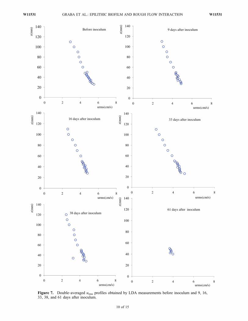
Figure 7. Double‐averaged urms profiles obtained by LDA measurements before inoculum and 9, 16,33, 38, and 61 days after inoculum.

GRABA ET AL.: EPILITHIC BIOFILM AND ROUGH FLOW INTERACTION W11531W11531

10 of 15

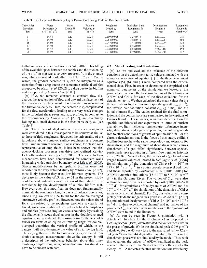
to that in the experiments of Nikora et al. [2002]. This fillingof the available space between the cobbles and the thickeningof the biofilm mat was also very apparent from the changein d, which increased gradually from 1.11 to 2.7 cm. On thewhole, the gradual decrease in ks can be interpreted as atransition from a drag due to the same nude artificial cobblesas reported byNikora et al. [2002] to a drag due to the biofilmmat as reported by Labiod et al. [2007].[37] If ks had remained constant at constant flow dis-

charge, the acceleration of flow and upward displacement ofthe zero‐velocity plane would have yielded an increase inthe friction velocity u*. Here, the decrease in ks compensatedfor the flow acceleration, leading to the very weak changesin the turbulent shear stress and urms profiles, in contrast tothe experiments by Labiod et al. [2007], and eventuallyleading to a small decrease in the friction velocity u* (seeTable 3).[38] The effects of algal mats on the surface roughness

were considered in this investigation to be somewhat similarto those of rigid roughness. However, the universality of theturbulence above complex surface roughness is a conten-tious issue in current research. For instance, for elastic rodsrepresentative of crop fields, it has been shown that fre-quency‐locking processes can drive well‐defined Kelvin‐Helmoltz vortices [see Py et al., 2006]. The same lock‐inmechanisms have been demonstrated for compliant wallsinteracting with a turbulent boundary layer [Xu et al., 2003].Strong modifications by an epilithic biofilm were notreported in the very detailed study by Nikora et al. [2002],most likely because they used low biomass systems. Thedecrease in the value of Du at day 61 in the present studycould indeed indicate a modification of the nature of theturbulence by the development of a thick biofilm mat.However even this modification does not fundamentallyeliminate the roughness length ks as a turbulence descriptor,since a log law can still be found for the double‐averagedstreamwise velocity profiles. However, how the values foundfor ks are related to the roughness geometry is clearly nottrivial, since contributions from wakes behind hemispheresand bubbles (pressure drag) or viscous boundary layers alongthe filaments (viscous drag) appear in the double‐averagedequations, and also decide the closure form for the Reynoldstensor (in terms of an equivalent mixing length for double‐averaged quantities, the vertical profile of which, in thecanopy, will also determine the value of ks in the log law).Thus, ks together with the friction velocity u*, extracted fromdouble‐averaged measurements above the canopy, is stilla descriptor of the turbulence behavior above this time‐evolving complex roughness, but methods used to estimate u*have to be chosen with care.

4.3. Model Testing and Evaluation

[39] To test and evaluate the influence of the differentequations on the detachment term, values simulated with thenumerical resolution of equation (1) for the three detachmentequations (5), (6), and (7) were compared with the experi-mental data. First, in order to determine the empirical andnumerical parameters of the simulation, we looked at theparameters that gave the best simulations of the changes inAFDM and Chl‐a for each of the three equations for thedetachment term. We then calculated the mean values for thethree equations for the maximum specific growth mmax (d

−1),the inverse half‐saturation constant kinv (g−1 m2), and theinitial biomass Binit. The values retained for the final simu-lation and the comparisons are summarized in the captions ofFigures 8 and 9. These values, which are dependent on thespecific conditions of our experiment in terms of nutrientavailability, light incidence, temperature, turbulence inten-sity, shear stress, and algal composition, cannot be general-ized to other conditions of growth of epilithic biofilm. For thechronic detachment that is the focus of this study, epilithicbiofilm does not have the same morphology and tolerance forshear stress, and the magnitude of shear stress which causesdetachment of algae differs significantly between species,particularly taxa growing in different flow regimes [Moulinet al., 2008a]. Nevertheless, the values of Cdet found con-verged toward values calibrated in Uehlinger et al. [1996]for simulations of the dynamics of Chl‐a (44 × 10−6 to149 × 10−3 s m−3 d−1) in a Swiss pre‐alpine gravel bed riverand those reported by Boulêtreau et al. [2006, 2008] forAFDM dynamics simulations (16 × 10−4 to 8 × 10−2 s m−3

d−1) in the Garonne River. The values of Cdet′′ were also

within the range of values reported by Fothi [2003] (0–67 ×10−4 d−1 for simulations of the dynamics of AFDM and 7 ×10−4 to 4 × 10−3 d−1 for simulations of the dynamics of Chl‐ain his experimental channel). For Cdet

′ our values were com-pletely outside the range values given in Labiod et al. [2007]in simulations of the dynamics of Chl‐a (2 × 10−3 to 4 × 10−3 sm−1 d−1 in their experimental channel) and no values of theparameterCdet

′ associated with simulations of the dynamics ofAFDM were found in the literature.[40] As can be seen in Figure 8, simulation with a

detachment function for the discharge Q as proposed byUehlinger et al. [1996] overestimated the values measured inthe phase of growth. While the simulated peak (30.9 g m−2)calculated for day 43 was close to the measured value (32.8 ±3.4 g m−2) reached 44 days after inoculum, the loss in thedetachment phase was not simulated by the model. Thus, withthis equation, the values of AFDM stabilized at the peakreached. The value of the Nash‐Sutcliffe coefficient of effi-ciency E = 0.35 indicates that this simulation is unsatisfactory

Table 3. Discharge and Boundary Layer Parameters During Epilithic Biofilm Growth

Time AfterInoculum(days)

WaterDischarge Q(10−3 m3 s−1)

WaterDepth H

(m)

FrictionVelocity u*

(m s−1)

RoughnessLength z0

(cm)

Equivalent SandRoughness ks

(cm)

DisplacementHeight d(cm)

RoughnessReynoldsNumber k+

0 14.44 0.13 0.028 0.109±0.005 3.27±0.15 1.11±0.03 9159 14.40 0.13 0.025 0.064±0.003 1.92±0.10 1.41±0.05 48016 14.50 0.13 0.024 0.047±0.001 1.41±0.04 1.64±0.09 33833 14.40 0.13 0.024 0.032±0.001 0.96±0.02 1.99±0.03 23038 14.42 0.13 0.023 0.028±0.001 0.84±0.04 2.26±0.18 19361 14.49 0.13 0.025 0.033±0.002 0.99±0.06 2.68±0.30 247

GRABA ET AL.: EPILITHIC BIOFILM AND ROUGH FLOW INTERACTION W11531W11531

11 of 15

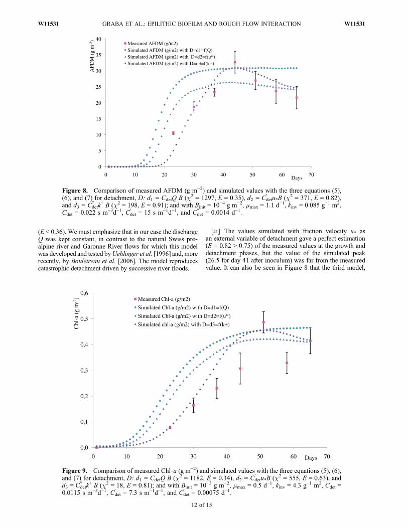
(E < 0.36). We must emphasize that in our case the dischargeQ was kept constant, in contrast to the natural Swiss pre‐alpine river and Garonne River flows for which this modelwas developed and tested byUehlinger et al. [1996] and, morerecently, by Boulêtreau et al. [2006]. The model reproducescatastrophic detachment driven by successive river floods.

[41] The values simulated with friction velocity u* asan external variable of detachment gave a perfect estimation(E = 0.82 > 0.75) of the measured values at the growth anddetachment phases, but the value of the simulated peak(26.5 for day 41 after inoculum) was far from the measuredvalue. It can also be seen in Figure 8 that the third model,

Figure 9. Comparison of measured Chl‐a (g m−2) and simulated values with the three equations (5), (6),and (7) for detachment, D: d1 = CdetQ B (c2 = 1182, E = 0.34), d2 = Cdet

′ u*B (c2 = 555, E = 0.63), andd3 = Cdet

′′ k+ B (c2 = 18, E = 0.81); and with Binit = 10−3 g m−2, mmax = 0.5 d−1, kinv = 4.3 g−1 m2, Cdet =0.0115 s m−3d−1, Cdet

′ = 7.3 s m−1d−1, and Cdet′′ = 0.00075 d−1.

Figure 8. Comparison of measured AFDM (g m−2) and simulated values with the three equations (5),(6), and (7) for detachment, D: d1 = CdetQ B (c2 = 1297, E = 0.35), d2 = Cdet

′ u*B (c2 = 371, E = 0.82),and d3 = Cdet

′′ k+ B (c2 = 198, E = 0.91); and with Binit = 10−4 g m−2, mmax = 1.1 d−1, kinv = 0.085 g−1 m2,Cdet = 0.022 s m−3d−1, Cdet

′ = 15 s m−1d−1, and Cdet′′ = 0.0014 d−1.

GRABA ET AL.: EPILITHIC BIOFILM AND ROUGH FLOW INTERACTION W11531W11531

12 of 15

with the roughness Reynolds number k+ (=u* ks/n) asexternal variable of detachment, gave a more accuratesimulation (E = 0.91) because the value of E is not onlygreater than 0.75, but also greater than the value found inthe simulation with friction velocity u* as an external vari-able of detachment. This is also confirmed by the decrease inthe value of conformity c2 with c2 = 1297 for d1 = CdetQ B;c2 = 371 for d2=Cdet

′ u*B; and c2 = 198 for d3=Cdet

′′ k+ B. Thesame tendencies can be observed in Figure 9, where theresults of simulated changes in Chl‐a (g m−2) are plottedalong with experimental data. Although the agreement wasnot as good as with AFDM, this could be because the AFDMbiomass descriptor gives a balance sheet of the total organicproduction and mortality, whereas Chl‐a only representsautotrophic production. The values of E and c2 found forthe Chl‐a simulations were E = 0.34 (unsatisfactory) andc2 = 1182 for d1=CdetQ B; E = 0.63 (satisfactory) and c2 =555 for d2=Cdet

′ u*B; and E = 0.81 (perfect) and c2 = 18 ford3=Cdet

′′ k+ B.[42] These results support the idea that transport phe-

nomena that occur in the near‐bed layer, such as chronicdetachment of epilithic biofilm matter or vertical transportof nutrients and pollutants in submerged aquatic canopies[Nepf et al., 2007], are not related to a single turbulencedescriptor such as the friction velocity u*, but require at leasttwo descriptors, here the friction velocity u* and the equiva-lent roughness height ks. In our study of chronic detachmentin the dynamics of epilithic matter, change in shear stress withthe age of the epilithic biofilm is considered through aparameter that integrates the bottom roughness dimensions:The Nikuradse equivalent sand roughness ks, which dependson the initial form and dimensions of the colonized substra-tum, and its changes owing to the thickness, resistance, andcomposition of the epilithic matter. This led us to concludethat the dynamics of epilithic matter can be better modeledand simulated by taking the roughness Reynolds number k+

as the external variable of the detachment.[43] In the literature, many different formulations have

been proposed to model the detachment. Some authors useempirical expressions, Horner et al. [1983] propose the termD = KV�, where V (cm s−1) is the mean current velocity andcould be easily replaced by the flow discharge Q, and � is anempirical power law. Other authors use terms associatedwith some assumptions on the physics of the process, forexample Saravia et al. [1998] propose the term dtBt(Vt −Vm)

2, where Vm (m s−1) is the mean current velocity duringbiofilmgrowth,Vt (m s−1) the actual current velocity,Bt (mgm

−2)the biomass, and dt (s

2 m−2) the degree of detachment pro-duced by an increase in velocity (measured byVt −Vm), with asquare power law relating the detachment to an excess ofkinetic energy. In the present study, we propose a term pro-portional to ks u*, a form that is closely related to simpleparameterizations of the vertical mass flux Φv from the can-opy layer to the external flow in turbulent boundary layersover roughness. For flows over urban canopies (e.g., windsover building‐like roughness), Bentham and Britter [2003]and Hamlyn and Britter [2005] introduced the concept ofexchange velocity UE to describe this vertical mass flux asΦv = UE(Cc −Cref), whereCref andCc are the concentrations inthe flow above and in the canopy, respectively. Those authorsshowed thatUE is proportional to the friction velocity u*, with afactor that depends on the difference in velocity between thecanopy layer and the flow above, that is, something indirectly

related to the roughness length z0 or, equivalently, to theroughness height ks. If biofilm parts in direct contact with theflow and available for detachment (detached or dead parts) arenow considered, their concentration in the canopy Cc will beproportional to the biomass quantity B, and far larger than theconcentration in the flow above (i.e., Cc − Cref ≈ B). Fol-lowing Bentham and Britter [2003], the vertical flux of bio-mass from the canopy to the flow above would then readΦv =f (ks)u*B, where f (ks) is a function of the roughness height ks,in agreement with the detachment term proposed in thepresent study. In other words, the chronic detachment can beseen as a permanent extraction by the hydrodynamics of somepart of the biomass that, together with the hemispheres, formsthe canopy sublayer. This parameterization is supported bygood agreement with the model developed by Nepf et al.[2007] for submerged aquatic canopies, where the verticalmass flux between the so‐called exchange zone (upper part ofthe canopy) and the flow above reads Φv = ke/de, with ke =0.19 u*(Cdah)

0.13 and de = 0.23h/(Cdah) obtained experimen-tally, yielding an expression reading Φv = 0.8u*(Cdah)

1.13,where Cd is the drag parameter for the plant rods and a theirdensity. Since Cdah is proportional to ks for sparse canopies,0.8(Cdah)

1.13 can be seen as the function f (ks) discussedabove. The equation proposed in the present paper, assumingproportionality with ks, is then in relatively good agreementwith the work of Nepf et al. [2007] and their 1.13 power law.

5. Conclusions

[44] In the present investigation, we tested the relevanceof three formulations for chronic detachment of epilithicbiofilm through numerical simulations with a simplifiedmodel adapted from Uehlinger et al. [1996]. In addition, weperformed experimental studies in an indoor open channelflow to measure the growth of epilithic biofilm in interactionwith turbulent rough flow and the evolution of local hydro-dynamic parameters during epilithic biofilm growth.[45] Laser Doppler anemometry measurements showed

that the presence and growth of epilithic matter affected thehydrodynamic characteristics by acceleration of the meanflow and by changes in the turbulence intensity and shearstress, especially at the flow‐biofilm interface. These changeswere evaluated by estimation of the friction velocity, Nikuradseequivalent sand roughness, and dimensionless roughnessReynolds number, which gave net smoothing of the bottomroughness with the presence and growth of epilithic biofilm.[46] Comparisons of the results of numerical simulations

with biological measurements revealed that chronic detach-ment was better simulated by taking the roughness Reynoldsnumber as the external variable of detachment. In fact, loss ofepilithic matter was related not only to local hydrodynamicconditions, but also to changes in bottom roughness, whichdepended on the amount of the biofilm matter present andits form, and which was well described by the Nikuradseequivalent sand roughness ks.[47] It is important to underline that turbulence and shear

stress not only control the detachment process, but also havea strong influence on the starting location of the colonizationprocess around the substrate, as well as the transfer rates ofnutrients, or carbon dioxide and oxygen, from the outerlayer to inside the biofilm. Thus, the influence of turbulenceand shear stress on the colonization and growth processescould be incorporated into future refinements of the model.

GRABA ET AL.: EPILITHIC BIOFILM AND ROUGH FLOW INTERACTION W11531W11531

13 of 15

Notation

A log law roughness geometries constant.AFDM ash free dry mass, g m−2.

B biomass, g m−2.Binit initial biomass, g m−2.C colonization function, g m−2 d−1.

Cdet, Cdet′ , and Cdet

′′ empirical detachment coefficients, s m−3

d−1, s m−1 d−1, and d−1, respectively.Chl‐a chlorophyll‐a, g m−2.

d displacement length, cm.D detachment function, g m−2 days−1.G growth function, g m−2 days−1.

kinv inverse half‐saturation constant, g−1m−2.ks Nikuradse equivalent sand roughness,

cm.k+ roughness Reynolds number (= u* ks/n).n number of acquisitions for a point of

measurement by laser Doppler ane-mometry.

SE standard error in measured values,g m−2.

U, V, W instantaneous velocity in the longitudi-nal, transversal, and vertical directionsrespectively, cm s−1.

U , V , W time‐averaged velocity in the longitudi-nal, transversal, and vertical directions,respectively, cm s−1.

hUixy double‐averaged longitudinal velocity,cm s−1.

u′, w′ root‐mean‐square value of longitudinal(urms) and vertical (wrms) velocity, res-pectively, cm s−1.

hu0w0ixy double‐averaged turbulent shear stress,cm2 s−2.

u* friction velocity, cm s−1 or m s−1.z distance from the flume bed, cm.z0 roughness length, cm.

mmax maximum specific growth, d−1.N water kinetic viscosity, 10−6 m2 s−1.D roughness height, cm.К Von Karma universal constant (к ≈ 0.4).

[48] Acknowledgments. Myriam Graba was supported by the Alger-ian Ministry of the Higher Education and the Scientific Research in frame ofthe national program of training abroad (PNE). This work was supported bythe national research project ACI‐FNS (ECCOEcosphère Continentale: Pro-cessus etModélisation) andwithin the framework of theGIS‐ECOBAG, Pro-gram P2 “Garonne Moyenne” supported by funds from CPER and FEDER(grant OPI2003‐768) of the Midi‐Pyrenees Region and Zone Atelier AdourGaronne) of PEVS/CNRS347 INSUE. We wish to thank A. Beer, S. Font,and G. Dhoyle for flume equipment and maintenance. We also thank anon-ymous reviewers for their critical comments.

ReferencesAsaeda, T., and D. Hong Son (2000), Spatial structure and populations of a

periphyton community: A model and verification, Ecol. Modell., 133,195–207, doi:10.1016/S0304-3800(00)00293-3.

Asaeda, T., and D. Hong Son (2001), A model of the development of aperiphyton community: Resource and flow dynamics, Ecol. Modell.,137, 61–75, doi:10.1016/S0304-3800(00)00432-4.

Auer, M. T., and R. P. Canale (1982), Ecological studies and mathematicalmodeling of Cladophora in Lake Huron: 3. The dependence of growthrates on internal phosphorus pool size, J. Great Lakes Res., 8, 93–99.

Belkhadir, R., B. Capdeville, and H. Roques (1988), Fundamental descrip-tive study and modelization of biological film growth: I. Fundamentaldescriptive study of biological film growth, Water Res., 22, 59–69.

Bentham, T., and R. Britter (2003), Spatially averaged flow over urban‐likeroughness, Atmos. Environ., 37, 115–125.

Biggs, B. J. F. (1996), Patterns in benthic algae of streams, in Algal Ecol-ogy: Freshwater Benthic Ecosystems, edited by R. J. Stevenson, M. L.Bothwell, and R. L. Lowe, pp. 31–56, Academic, San Diego, Calif.

Biggs, B. J. F., and C. W. Hickey (1994), Periphyton responses to ahydraulic gradient in a regulated river in New Zealand, Freshwater Biol.,32, 49–59.

Bothwell, M. L., D. Sherbot, A. C. Roberge, and R. J. Daley (1993), Influ-ence of natural ultraviolet radiation on lotic periphytic diatom communitygrowth, biomass accrual, and species composition: Short‐term versuslong‐term effects, J. Phycol., 29, 24–35.

Boulêtreau, S., F. Garabetian, S. Sauvage, and J. M. Sánchez‐Pérez (2006),Assessing the importance of self‐generated detachment process in riverbiofilm models, Freshwater Biol., 51, 901–912, doi:10.1111/j.1365-2427.2006.01541.x.

Boulêtreau, S., O. Izagirre, F. Garabetian, S. Sauvage, A. Elosegi, and J. M.Sánchez‐Pérez (2008), Identification of a minimal adequate model todescribe the biomass dynamics of river epilithon, River Res. Applic.,24, 36–53, doi:10.1002/rra.1046.

Borchardt, M. A. (1996), Nutrients, in Algal Ecology: Freshwater BenthicEcosystems, edited by R. J. Stevenson, M. L. Bothwell, and R. L. Lowe,pp. 183–227, Academic, San Diego, Calif.

Capdeville, B., R. Belkhadir, and H. Roques (1988), Fundamental descrip-tive study and modelization of biological film growth: I. A new conceptof biological film growth modelization, Water Res., 22, 71–77.

Cheng, H., and I. P. Castro (2002), Near‐wall flow over urban‐like rough-ness, Boundary Layer Meteorol., 104, 229–259.

Flipo, N., S. Even, M. Poulin, M. H. Tusseau‐Vuillemin, T. Ameziane, andA. Dauta (2004), Biogeochemical modeling at the river scale: Planktonand periphyton dynamics, Grand Morin case study, France, Ecol. Modell.,176, 333–347, doi:10.1016/j.ecolmodel.2004.01.012.

Fothi, A. (2003), Effets induits de la turbulence benthique sur les méca-nismes de croissance du périphyton, Ph.D. dissertation, Inst. Natl. Poly-tech. de Toulouse, Toulouse, France.

Fuller, R. L., J. L. Roelofs, and T. J. Frys (1986), The importance of algaeto stream invertebrates, J. N. Am. Benthol. Soc., 5, 290–296.

Ghosh, M., and J. P. Gaur (1998), Current velocity and the establishment ofstream algal periphyton communities, Aquat. Bot., 60, 1–10.

Godillot, R., T. Ameziane, B. Caussade, and J. Capblanc (2001), Inter-play between turbulence and periphyton in rough open‐channel flow,J. Hydraul. Res., 39, 227–239.

Hamlyn, D., and R. Britter (2005), A numerical study of the flow field andexchange processes within a canopy of urban‐like roughness, Atmos.Environ., 39, 3243–3254.

Hart, D., and C. M. Finelli (1999), Physical‐biological coupling in streams:The pervasive effects of flow on benthic organisms, Annu. Rev. Ecol.Syst., 30, 363–395.

Hondzo, M., and H. Wang (2002), Effects of turbulence on growth andmetabolism of periphyton in a laboratory flume, Water Resour. Res.,38(12), 1277, doi:10.1029/2002WR001409.

Horner, R. R., and E. B. Welch (1981), Stream periphyton development inrelation to current velocity and nutrients, Can. J. Fish. Aquat. Sci., 38,449–457.

Horner, R. R., E. B. Welch, and R. B. Veenstra (1983), Development ofnuisance periphytic algae in laboratory streams in relation to enrichmentand velocity, in Periphyton of Freshwater Ecosystems, pp. 121–164, editedby R. G. Wetzel, Dr. W. Junk, The Hague, Netherlands.

Jeffrey, S. W., R. F. C. Mantoura, and S. W. Wright (1997), PhytoplanktonPigments in Oceanography: Guidelines to Modern Methods, 661 pp.,UNESCO, Paris.

Kliment, Z., J. Kadlec, and J. Langhhammer (2008), Evaluation of sus-pended load changes using AnnAGNPS and SWAT semi‐empirical erosionmodels, Catena, 73, 286–299, doi:10.1016:j.catena.2007.11.005.

Krause, P., D. P. Boyle, and F. Base (2005), Comparison of different effi-ciency criteria for hydrological model assessment, Adv. Geosci., 5, 89–97.

Labiod, C., R. Godillot, and B. Caussade (2007), The relationship betweenstream periphyton dynamics and near‐bed turbulence in rough open‐channelflow, Ecol. Modell., 209, 78–96, doi:10.1016/j.ecolmodel.2007.06.011.

Lekfir, A., T. A. Benkaci, and N. Dechemi (2006), Quantification du trans-port solide par la technique floue, application au barrage de Béni Amrane(Algérie), Rev. Sci. Eau, 19, 247–257.

Lock, M. A., R. R. Wallace, J. W. Costerton, R. M. Ventullo, and S. E.Charlton (1984), River epilithon: Toward a structural‐functional model,Oikos, 42, 10–22.

GRABA ET AL.: EPILITHIC BIOFILM AND ROUGH FLOW INTERACTION W11531W11531

14 of 15

Lopez, F., and M. Garcia (1998), Open‐channel flow through simulatedvegetation: Suspended sediment transport modeling, Water Resour.Res., 34, 2341–2352.

Lopez, F., and M. Garcia (2001), Mean flow and turbulence structure ofopen‐channel flow through nonemergent vegetation, J. Hydraul. Eng.,127, 392–402.

Mayer, M. S., and G. E. Likens (1987), The importance of algae in ashaded headwater stream as a food of an abundant caddisfly (Trichoptera),J. N. Am. Benthol. Soc., 6, 262–269.

McIntire, C. (1973), Periphyton dynamics in laboratory streams: A simula-tion model and its implications, Ecol. Monogr., 34, 399–420.

McLean, S., and V. I. Nikora (2006), Characteristics of turbulent unidirec-tional flow over rough beds: Double‐averaging perspective with partic-ular focus on sand dunes and gravel bed, Water Resour. Res., 42,W10409, doi:10.1029/2005WR004708.

Mignot, E., E. Barthelemy, and D. Hurther (2009), Double‐averaging anal-ysis and local flow characterization of near‐bed turbulence in gravel‐bed channel flows, J. Fluid Mech., 618, 279–303, doi:10.1017/S0022112008004643.

Minshall, G. W. (1978), Autotrophy in stream ecosystems, BioScience, 28,767–771.

Momo, F. (1995), A new model for periphyton growth in running waters,Hydrobiologia, 299, 215–218.

Moulin, F. Y., et al. (2008a), Experimental study of the interaction betweena turbulent flow and a river biofilm growing on macrorugosities, inAdvances in Hydro‐Science and Engineering, vol. 8, edited by S. S.Y. Wang, pp. 1887–1896, Int. Assoc. Hydro‐Environ. Eng. Res.,Nagoya, Japan.

Moulin, F. Y., K. Mülleners, C. Bourg, and S. Cazin (2008b), Experimentalstudy of the impact of biogenic macrorugosities on the benthic boundarylayer, in Advances in Hydro‐Science and Engineering, vol. 8, edited byS. S. Y. Wang, pp. 736–745, Int. Assoc. Hydro‐Environ. Eng. Res.,Nagoya, Japan.

Nepf, H., M. Ghisalberti, B. White, and E. Murphy (2007), Retention timeand dispersion associated with submerged aquatic canopies, WaterResour. Res., 43, W04422, doi:10.1029/2006WR005362.

Nezu, I., and H. Nakagawa (1993), Turbulence in Open‐Channel Flows,Balkema, Rotterdam, Netherlands.

Nielsen, T. S., W. H. Funk, H. L. Gibbons, and R. M. Duffner (1984), Acomparison of periphyton growth on artificial and natural substrates inthe upper Spokane River, Northwest Sci., 58, 243–248.

Nikora, V., D. Goring, and B. Biggs (1997), On stream periphyton‐turbulence interactions, N. Z. J. Mar. Freshwater Res., 31, 435–448.

Nikora, V., D. Goring, and B. Biggs (1998), A simple model of streamperiphyton‐flow interactions, Oikos, 81, 607–611.

Nikora, V., D. Goring, I. McEwan, and G. Griffiths (2001), Spatially aver-aged open‐channel flow over rough bed, J. Hydraul. Eng., 127, 123–133.

Nikora, V., D. Goring, and B. Biggs (2002), Some observations of theeffects of microorganisms growing on the bed of an open channel onthe turbulence properties, J. Fluid Mech., 450, 317–341.

Nikora, V., I. McEwan, S. McLean, S. Coleman, D. Pokrajac, and R.Walters(2007a), Double averaging concept for rough‐bed open‐channel and over-

land flows: Theoretical background, J. Hydraul. Eng., 133, 873–883,doi:10.1061/(ASCE)0733-9429(2007)133:8(873).

Nikora, V., S. McLean, S. Coleman, D. Pokrajac, I. McEwan, L. Campbell,J. Aberle, D. Clunie, and K. Kol (2007b), Double‐averaging concept forrough‐bed open‐channel and overland flows: Applications background,J. Hydraul. Eng., 133, 884–895, doi:10.1061/(ASCE)0733-9429(2007)133:8(884).

Py, C., E. de Langre, and B. Moulia (2006), A frequency lock‐in mecha-nism in the interaction between wind and crop canopies, J. Fluid Mech.,568, 425–449, doi:10.1017/S0022112006002667.

Reiter, M. A. (1986), Interactions between the hydrodynamics of flowingwater and development of a benthic algal community, J. FreshwaterEcol., 3, 511–517.

Reiter, M. A. (1989a), Development of benthic algal assemblages subjectedto differing near‐substrate hydrodynamic regimes, Can. J. Fish. Aquat.Sci., 46, 1375–1382.

Reiter, M. A. (1989b), The effect of a developing algal assemblage on thehydrodynamics near substrates of different size, Arch. Hydrobiol., 115,221–244.

Saravia, L., F. Momo, and L. D. Boffi Lissin (1998), Modeling periphytondynamics in running water, Ecol. Modell., 114, 35–47.

Stevenson, R. J. (1983), Effects of currents and conditions simulatingautogenically changing microhabitats on benthic diatom immigration,Ecology, 64, 1514–1524.

Stevenson, R. J. (1996), An introduction to algal ecology in freshwater ben-thic habitats, in Algal Ecology: Freshwater Benthic Ecosystems, edited byR. J. Stevenson,M. L. Bothwell, and R. L. Lowe, pp. 3–30, Academic, SanDiego, Calif.

Uehlinger, U., H. Buhrer, and P. Reichert (1996), Periphyton dynamics in aflood prone pre‐alpine river: Evaluation of significant processes by mod-eling, Freshwater Biol., 36, 249–263.

Wilcock, P. (1996), Estimating local bed shear stress from velocity obser-vations, Water Resour. Res., 32, 3361–3366.

Winterbourn, M. J. (1990), Interactions among nutrients, algae, andinvertebrates in a New Zealand mountain stream, Freshwater Biol.,23, 463–474.

Xu, S., D. Rempfer, and J. Lumley (2003), Turbulence over a compliantsurface: Numerical simulation and analysis, J. Fluid Mech., 478, 11–34,doi:10.1017/S0022112002003324.

S. Boulêtreau, J. M. Sánchez‐Pérez, and S. Sauvage, ECOLAB, Universitéde Toulouse, UPS, INPT, CNRS, Avenue de l’Agrobiopôle, BP 32607,Auzeville‐Tolosane, Castanet‐Tolosan, F‐31326 Toulouse, France.(sabine.sauvage@ensat.fr)O. Eiff and F. Y. Moulin, IMFT, Université de Toulouse, UPS, INPT,

ENSEEIHT, CNRS, F‐31400 Toulouse, France.F. Garabétian, UMR 5805, Station Marine d’Arcachon, EPOC‐OASU,

Université Bordeaux 1, 2 Rue du Professeur Jolyet, F‐33120 ArcachonCEDEX, France.M. Graba and A. Kettab, Laboratoire des Sciences de l’Eau, Ecole

Nationale Polytechnique, 10 Ave. Hassen Badi, El Harrach, Alger 16200,Algeria.

GRABA ET AL.: EPILITHIC BIOFILM AND ROUGH FLOW INTERACTION W11531W11531

15 of 15