Efficiency of an auto-propelled flapping airfoil

Contents lists available at ScienceDirect

Journal of Fluids and Structures

Journal of Fluids and Structures 27 (2011) 552–566

0889-97

doi:10.1

n Corr

E-m

journal homepage: www.elsevier.com/locate/jfs

Efficiency of an auto-propelled flapping airfoil

T. Benkherouf a, M. Mekadem a, H. Oualli a, S. Hanchi a,n, L. Keirsbulck b, L. Labraga b

a LMDF Ecole Militaire Polytechnique (EMP), BP17 Bordj-el-Bahri, 16111 Algiers, Algeriab LME, UVHC, 59313 Valenciennes Cedex 9, France

a r t i c l e i n f o

Article history:

Received 19 April 2010

Accepted 7 March 2011Available online 11 April 2011

Keywords:

Self-propulsion

Flapping airfoils

Propulsive efficiency

46/$ - see front matter & 2011 Elsevier Ltd. A

016/j.jfluidstructs.2011.03.004

esponding author.

ail address: [email protected] (S. Hanch

a b s t r a c t

The present study deals with an investigation of the flow aerodynamic characteristics

and the propulsive velocity of a system equipped with a nature inspired propulsion

system. In particular, the study is aimed at studying the effect of the flapping frequency

on the flow behavior. We consider a NACA0014 airfoil undergoing a vertical sinusoidal

flapping motion. In contrast to nearly all previous studies in the literature, the present

work does not impose any velocity on the inlet flow. During each iteration the outer

flow velocity is computed after having determined the forces exerted on the airfoil.

Forward motion may only be produced by flapping motion of the airfoil. This is more

consistent with the physical phenomenon. The non-stationary viscous flow around the

flapping airfoil is simulated using Ansys-Fluent 12.0.7. The airfoil movement is achieved

using the deformable mesh technique and an in-house developed User Define Function

(UDF). Our results show the influence of flapping frequency and amplitude on both the

airfoil velocity and the propulsive efficiency. The resulting motion is contrasts to the

applied forces. In the present study, the frequency ranges from 0.1 to 20 Hz while the

airfoil amplitude values considered are: 10%, 17.5%, 25% and 40%.

& 2011 Elsevier Ltd. All rights reserved.

1. Introduction

Flying and swimming animals use their body and member movements as a means of displacement in the air and water,respectively. What allows for this extraordinary mobility has been subject of many studies during the past years, butunderstanding the mechanisms involved and controlling them still remains a complicated tasks. Experiments are hard toset up owing to the fact that equipping an animal with measurement probes often disturbs the animals’ behavior.

The first tentative explanations concerning the mechanisms of lift and propulsion by flapping were proposed in 1909(Knoller, 1909) and 1912 (Betz, 1912). The Knoller–Betz effect stipulates that insects produce a propulsion force byachieving a sinusoidal distribution of the angle of attack during the flapping movement. The main property of the flowassociated with an oscillating movement is the existence of a pair of asymmetric vortices, which are located in the vicinityof the leading edge on both the extrados and the intrados. During the flapping movement, the vortices are pushed towardsthe trailing edge where they are ejected, thus, initiating the formation of a vortex street.

While a steady swimming fish moves its body or fins in the water, muscle contraction, nervous system control alongwith interaction between the body tissues and the surrounding fluid contribute to the efficient and agile motion (Yu et al.,2008). Among the fish swimming, the carangiform swimmer has the ability of maintaining high-speed swimming in calmwaters, whereas the anguilliform swimmer exhibits remarkable maneuverability in cluttered environments (Sfakiotakiset al., 1999).

ll rights reserved.

i).

www.elsevier.com/locate/jfs

dx.doi.org/10.1016/j.jfluidstructs.2011.03.004

mailto:[email protected]

dx.doi.org/10.1177/0142331208090045

Nomenclature

c airfoil chordCDp drag coefficientCL lift coefficientCp period-averaged consumption power rate

coefficientCt period-averaged thrust powerDt time stepV-

center of mass velocityF-

global force per unit spanf flapping frequencyFx longitudinal projection of the global forceFxp generated pressure force in the x-direction

(longitudinal)Fy transversal projection of the global forceFy instantaneous generated force component in

the normal-direction (transversal)H near wall cell heighth instantaneous airfoil positionh0 non-dimensional maximal amplitude of the

flapping movementHideal near wall ideal cell height

Hmin near wall minimum cell heightkG Garrick reduced frequency ðpf=uÞ

m mass of the bodyRe Reynolds number (based on constant imposed

inlet velocity) ðrUec=mÞRex Reynolds number (based on airfoil velocity)

ðruc=mÞRexm steady-state Reynolds number (based on air-

foil velocity)t timeu longitudinal projection of the center of mass

velocityU longitudinal velocity of body center of massUe constant imposed inlet velocityv transversal projection of the center of mass

velocityx streamwise direction (longitudinal)y vertical direction (normal)as layer split factorZ propulsive efficiencyr densitym viscositys reduced frequency ð2pf=UÞ

T. Benkherouf et al. / Journal of Fluids and Structures 27 (2011) 552–566 553

Fish and Lauder (2006) were interested in fish as well as biological control mechanisms of aquatic mammals flow. Thisis an area having a long history and lots of results reflecting the increasing interest of researchers towards understandinghow organisms control the flow around their bodies and their tubercles. Fish and Lauder (2006) identified research areauseful to understanding of the non-stationary nature of the movement.

Prangemeier et al. (2010) investigated using particle image velocimetry (PIV) the manipulation of trailing-edge vortexfor an airfoil undergoing harmonic plunging superimposed with a pitching motion near the bottom of the stroke (theso-called quick-pitch motion). It has been shown that the trailing-edge vortex circulation can be reduced by more than 60%for all quick-pitch cases compared with a benchmark pure-sinusoidal plunge motion.

A comprehensive review of the biological and hydrodynamic literature of the aspects of aquatic locomotion wasprovided in Bandyopadhyay (2004), Fish (2004), Lauder (2005) Lauder and Drucker (2004), Triantafyllou et al. (2000,2004), Webb (1998) and Wilga and Lauder (2004).

Postlethwaite et al. (2008) studied a model for the optimal movement of an electric fish searching for a prey. The modelhas six degrees of freedom, which allows for movements that the real fish cannot execute. However, the results haveshown that the optimized trajectories are those made by the real fish.

In the flying area Hoa et al. (2003) reviewed the laws and the instationary modes for aerial biological and syntheticvehicles. Hoa et al. (2003) present an explanation for the aerodynamic gain of the flexible wings compared to the rigidwings. They also develop a three-dimensional non-stationary CFD code with an integrated distributed algorithm. Theresults of their model show that the flexible membranes improve both lift and thrust not by maximizing the force positivepeaks, but rather by reducing the negative minima.

Lin et al. (2006) carried out wind tunnel tests to measure the lift and the thrust of a membrane wing flappingmechanically with various frequency, velocity and angle of attack values. They observe that the wing structure flexibilityaffects the thrust and the lift due to its deformation for high flapping frequencies. For a constant speed, the lift forceincreases with flapping frequency. For a constant flapping frequency, the flight velocity can be increased by decreasingangle of attack while losing slightly on the lift force. Mazaheri and Ebrahimi (2010) use an experimental apparatus toinvestigate the effects of a wing’s twisting stiffness on the generated thrust force and the power required at differentflapping frequencies. The results show the manner in which the elastic deformation and inertial flapping forces affect thedynamical behavior of the wing.

Some prototypes using fish-like propulsion are now available. Among others, we mention the work of Yu et al. (2009),which addresses the design, construction, and motion control of an adjustable Scotch yoke mechanism replicating thekinematics of dolphin-like robots. Preliminary tests in a robotics context confirm the feasibility of this devised mechanismfor use as a propulsor for bio-inspired movements. Low (2009) considers and discusses the biomimetic design and theworkspace study of undulating fin propulsion mechanisms. He also presents examples for the BCF fish and the roboticcounterpart developed in different laboratories and manufacturers around the world.

The present study focuses on the estimation of the aerodynamic flow characteristics and the propulsion velocity of amachine equipped with a nature inspired propulsion system. This is done by implementing in the Ansys-Fluent software

T. Benkherouf et al. / Journal of Fluids and Structures 27 (2011) 552–566554

package the tools necessary to study the involved phenomena and get insight in problems relating to the aquatic and flyinglocomotion using the flapping dynamic of wings and fins. Fish and insects exhibit a wide range of body geometrydeformation configuration. In these swimming or flying models, there are many unresolved open questions. This includesthe propulsion and the maneuvering mechanisms which are at the basis of the remarkable maneuverability observed forsome species, the propulsive rate of swimming dynamic and both the stability and control of the fish movement. Theanswers to these fundamental questions may also help in interpreting the shape evolution of fish and insects.

2. Numerical procedure

2.1. Governing equations

The numerical simulations are carried out using Ansys-Fluent 12.0.16. The pressure coupled solver is used to solve theNavier–Stokes equations with a CFL equal to 1. The algorithm solves the coupled momentum and pressure basedcontinuity equation simultaneously. The full implicit coupling is obtained from an implicit discretisation of the pressuregradient terms in the momentum equations and an implicit discretisation of the mass flux on the cell faces, which includesthe dissipation terms of Rhie and Chow (1983). The flow is considered laminar in all simulations. The 3rd order MUSCLconvective scheme (Van Leer, 1979) (Monotone Upstream-Centered Schemes for Conservation Laws) is used to discretizeall transport equations. It is built from the mixing of a centered differentiation scheme and a second order upwind scheme.The MUSCL scheme applies to any type of mesh. Compared to the second order upwind scheme, the MUSCL schemeimproves the spatial precision by reducing the numerical diffusion.

2.2. Motion modeling and deformable mesh

The present study simulates the flapping motion of a NACA0014 airfoil with maximum flapping amplitude rangingfrom 10% to 40% of the chord and flapping frequency in the interval [0.1–20] Hz.

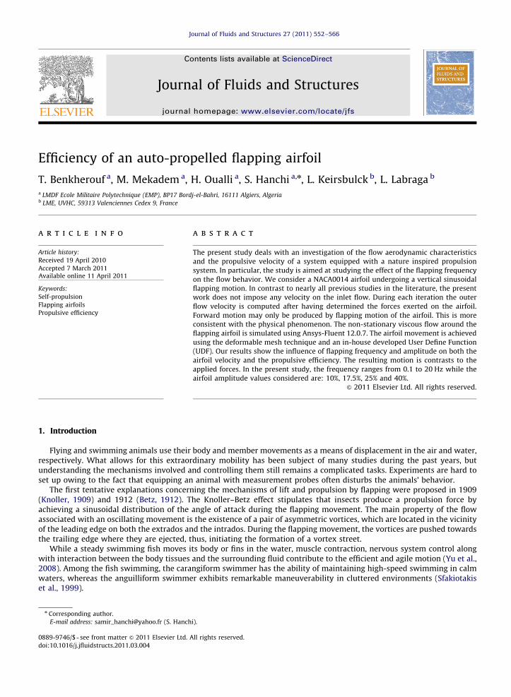
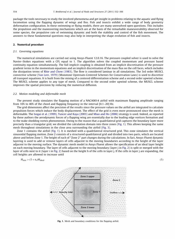
The grid dimensions affect the precision of the results since the pressure values on the airfoil are integrated to calculatepropulsion forces which induce the body displacement. The effect of the grid is even more pronounced since the mesh isdeformable. The Isogai et al. (1999), Tuncer and Kaya (2003) and Miao and Ho (2006) strategy is used. Indeed, as reportedby these authors the aerodynamic forces of a flapping wing are essentially due to the leading edge vortices formation andto the wake shedding vortex phenomenon. Owing to the reason that a quadrilateral grid captures the boundary layer moreprecisely than a triangular grid, we divided the calculation domain into three zones (Fig. 1). This allows keeping the samemesh throughout simulations in the close area surrounding the airfoil (Fig. 3).

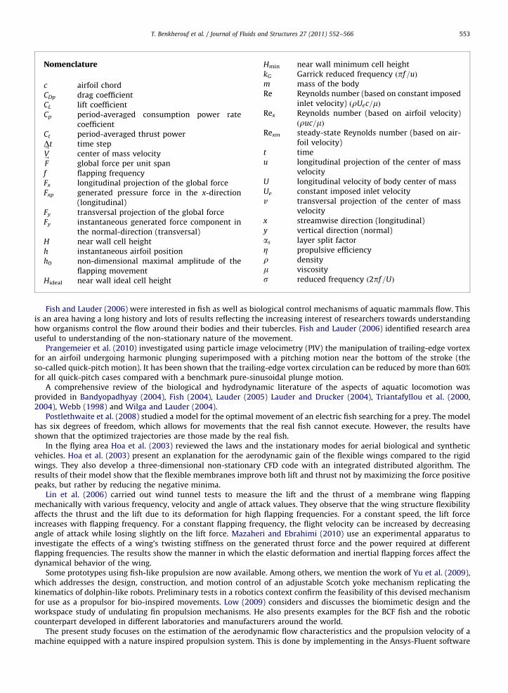
Zone 1 contains the airfoil (Fig. 1). It is meshed with a quadrilateral structured grid. This zone simulates the verticalsinusoidal flapping motion. Zone 2 consists of a structured quadrilateral grid and divided into two parts, which are locatedabove and below Zone 1. The height of each of ‘‘Zone 2’’ part changes during the calculations. In fact, Ansys-Fluent dynamiclayering is used to add or remove layers of cells adjacent to the moving boundaries according to the height of the layeradjacent to the moving surface. The dynamic mesh model in Ansys Fluent allows the specification of an ideal layer heighton each moving boundary. The layer of cells adjacent to the moving boundary (layer j in Fig. 2) is split or merged with thelayer of cells next to it (layer i in Fig. 2) based on the height h of the cells in layer j. If the cells in layer j are expanding, thecell heights are allowed to increase until

Hmin4ð1þasÞHideal: ð1Þ

Velocity Inlet Zone 1

Zone 2 upper

Zone 2 lower

Zone 3

Fig. 1. Mesh and boundary conditions for the flapping airfoil.

H

Layer i

Layer j

Moving boundary

Fig. 2. Mesh near a moving boundary.

t = t t = t + T/5 t = t + 2T/5

t = t + 3T/5 t = t + 4T/5 t = t + T

Zone 1 Zone 1 Zone 1

Zone 1 Zone 1 Zone 1

Zone 2upper

Zone 2lower

Zone 2upper

Zone 2upper

Zone 2lower

Zone 2lower

Zone 2upper

Zone 2upper

Zone 2upper

Fig. 3. Zone 1 and Zone 2 evolutions during the layering process for flapping airfoil.


If the cells in layer j are compressing, the cell heights are allowed to decrease until

Hmino ð1�asÞHideal, ð2Þ

where Hmin is the minimum cell height of cell layer j, Hideal is the ideal cell height, and as is the layer split factor.At every temporal iteration, the grid of ‘‘Zone 2’’ is recomputed to take into account the airfoil flapping. The airfoil

velocity, which results from the aerodynamic forces, is then estimated and introduced as a velocity inlet boundarycondition (instead of moving the foil backwards or forwards).

The considered mesh consists of 16,300 quadrilateral cells and 5056 triangular cells. The interface between the threezones is modeled as a conformal mesh to ensure the flux conservation for all the variables (Fig. 1). The height of the cells incontact with the airfoil is constant and equal to 0.2 mm. According to Tuncer and Kaya (2003) and Miao and Ho (2006),this mesh is sufficiently dense and fine in the vicinity of the wall to catch both boundary layer and wake. The flappingmovement is governed by the following law:

h¼ h0ccosð2pftÞ, ð3Þ

where h is the instantaneous airfoil position along the y axis, h0 the maximal amplitude of the flapping movement, c theairfoil chord, f the flapping frequency, and t the time.

2.3. Fluid motion coupling

An oscillating body in forward motion at a regular speed, which undergoes a flapping movement, may produce a thrustunder suitable parametric conditions. The thrust is produced when the time average of the body downstream flow has a jetform. On the other hand, if the flow is subject to drag forces, it will have a friction wake shape. In both cases, large powervortices develop in the wake. Their shapes depend on the parametric choices shown by several researchers usingvisualizations (Oshima and Oshima, 1980; Oshima and Natsume, 1980; Freymuth, 1988; Anderson et al., 1998). The two-dimensional flow studies showed that the downstream flow can be characterized by the formation of a sinuous wake i.e. awake which has either two or four large vortices per time period. A high propulsive efficiency is associated with theformation of two vortices per cycle which form a shifted raw of vortices similar to a Von-Karman eddy street. In this casethe vortices turn in opposite direction comparative with the classical Von-Karman eddy street (Triantafyllou et al., 2000).

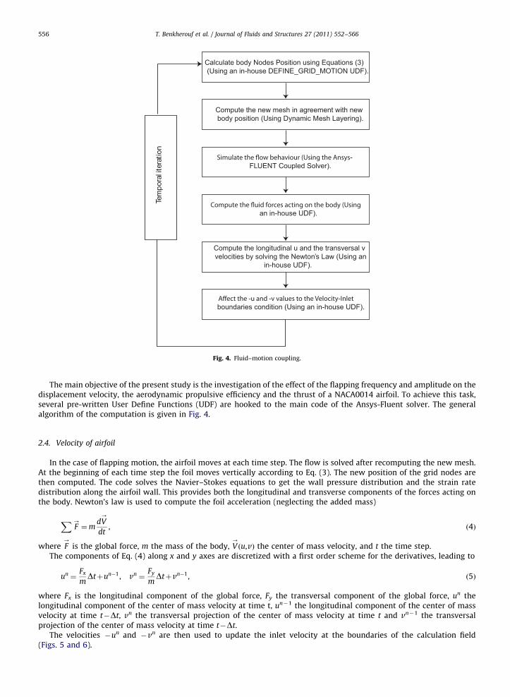
Calculate body Nodes Position using Equations (3) (Using an in-house DEFINE_GRID_MOTION UDF).

Compute the new mesh in agreement with new body position (Using Dynamic Mesh Layering).

-FLUENT Coupled Solver).

an in-house UDF).

Compute the longitudinal u and the transversal v velocities by solving the Newton’s Law (Using an

in-house UDF).

boundaries condition (Using an in-house UDF).

Tem

pora

lite

ratio

n

Fig. 4. Fluid–motion coupling.


The main objective of the present study is the investigation of the effect of the flapping frequency and amplitude on thedisplacement velocity, the aerodynamic propulsive efficiency and the thrust of a NACA0014 airfoil. To achieve this task,several pre-written User Define Functions (UDF) are hooked to the main code of the Ansys-Fluent solver. The generalalgorithm of the computation is given in Fig. 4.

2.4. Velocity of airfoil

In the case of flapping motion, the airfoil moves at each time step. The flow is solved after recomputing the new mesh.At the beginning of each time step the foil moves vertically according to Eq. (3). The new position of the grid nodes arethen computed. The code solves the Navier–Stokes equations to get the wall pressure distribution and the strain ratedistribution along the airfoil wall. This provides both the longitudinal and transverse components of the forces acting onthe body. Newton’s law is used to compute the foil acceleration (neglecting the added mass)

XF-¼m

dV-

dt, ð4Þ

where F-

is the global force, m the mass of the body, V-

ðu,vÞ the center of mass velocity, and t the time step.The components of Eq. (4) along x and y axes are discretized with a first order scheme for the derivatives, leading to

un ¼Fx

mDtþun�1, vn ¼

Fy

mDtþvn�1, ð5Þ

where Fx is the longitudinal component of the global force, Fy the transversal component of the global force, un thelongitudinal component of the center of mass velocity at time t, un�1 the longitudinal component of the center of massvelocity at time t�Dt, vn the transversal projection of the center of mass velocity at time t and vn�1 the transversalprojection of the center of mass velocity at time t�Dt.

The velocities �un and �vn are then used to update the inlet velocity at the boundaries of the calculation field(Figs. 5 and 6).

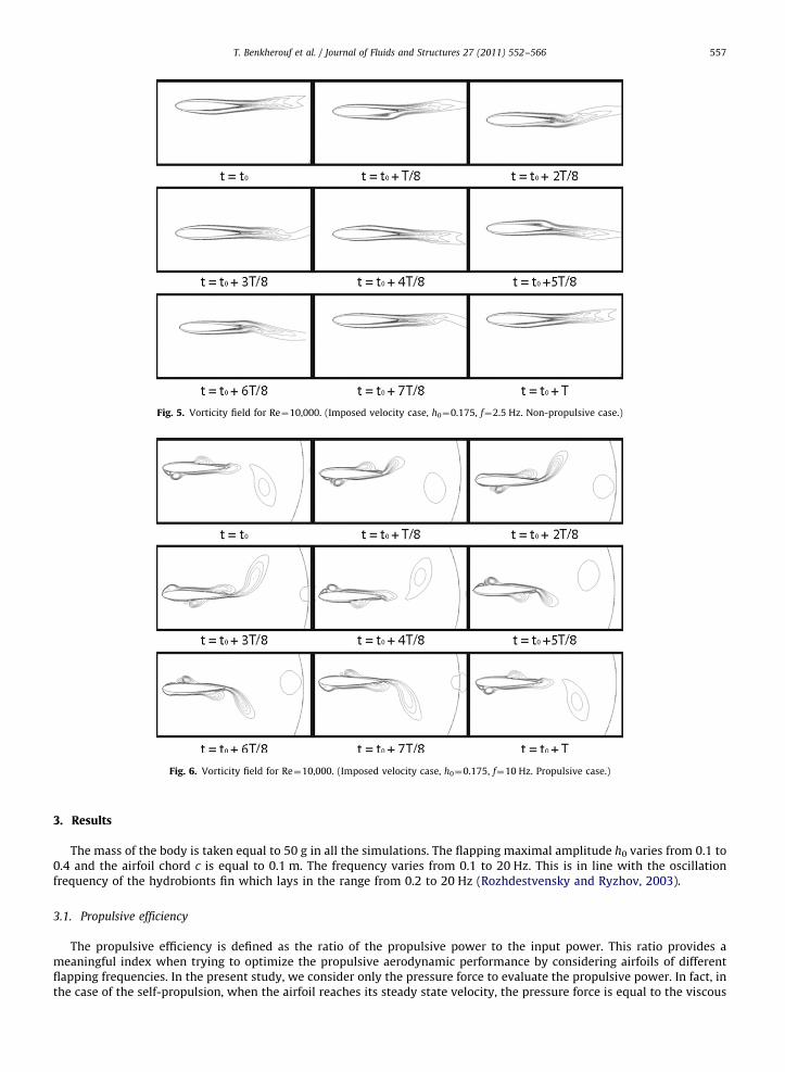
Fig. 5. Vorticity field for Re¼10,000. (Imposed velocity case, h0¼0.175, f¼2.5 Hz. Non-propulsive case.)

Fig. 6. Vorticity field for Re¼10,000. (Imposed velocity case, h0¼0.175, f¼10 Hz. Propulsive case.)


3. Results

The mass of the body is taken equal to 50 g in all the simulations. The flapping maximal amplitude h0 varies from 0.1 to0.4 and the airfoil chord c is equal to 0.1 m. The frequency varies from 0.1 to 20 Hz. This is in line with the oscillationfrequency of the hydrobionts fin which lays in the range from 0.2 to 20 Hz (Rozhdestvensky and Ryzhov, 2003).

3.1. Propulsive efficiency

The propulsive efficiency is defined as the ratio of the propulsive power to the input power. This ratio provides ameaningful index when trying to optimize the propulsive aerodynamic performance by considering airfoils of differentflapping frequencies. In the present study, we consider only the pressure force to evaluate the propulsive power. In fact, inthe case of the self-propulsion, when the airfoil reaches its steady state velocity, the pressure force is equal to the viscous


force. The only work provided by the airfoil is the one that will balance the viscous forces. So, only the pressure forces areneeded to calculate the propulsive power.

The drag and the lift coefficients are defined, respectively, as

CDpðtÞ ¼

FxpðtÞ

ð1=2ÞrðUðtÞÞ2c, CLðtÞ ¼

FyðtÞ

ð1=2ÞrðUðtÞÞ2c, ð6Þ

where UðtÞ is the longitudinal velocity of body center of mass, FyðtÞ and FxpðtÞ represent, respectively, the instantaneousgenerated force component in the normal-direction (transversal) and the generated pressure force in the x-direction(longitudinal), t, the time, and c the airfoil chord.

The period-averaged consumption power rate (CP) and the thrust power (Ct) can be evaluated, respectively, as

Cp ¼fR tn þ1=f

tnFyðtÞ dh

dt dt

ð1=2ÞrðUmÞ3c

, Ct ¼fR tn þ1=f

tnFxpðtÞUVxðtÞdt

ð1=2ÞrðUmÞ3c

, ð7Þ

where dh=dt is the traveling velocity of the flapping motion, Um is the imposed-velocity (in the imposed velocity case) orthe average steady state value of forward velocity (in the auto-propulsive case) and [tn, (tnþ1/f)] is the last period offlapping.

The propulsive efficiency is then defined as

Z¼ Ct

Cp: ð8Þ

3.2. Validation

In nearly all previous studies, the Reynolds number is imposed at the inlet of the computational domain (except in thework of Leroyer and Visonneau, 2005). In the present study, no velocity is imposed at the inlet boundary and the velocityof the airfoil is a computational result obtained by self-propulsion.

To improve the grid and the proposed method we compare our results to those of Heathcote et al. (2008), whichconsists of a water tunnel experimental study of the effect of span wise flexibility on the thrust, lift and propulsion of arectangular wing oscillating in pure heave. The inlet velocity is imposed and the Reynolds number takes the followingvalues: 10,000, 20,000 and 30,000. For conformity with the experiment of Heathcote, the in-house made ‘‘User DefinedFunction’’ is only used to carry out the foil motion and to estimate the real foil velocity motion without reintroducing it asan inlet velocity. The inlet velocity is imposed by the Reynolds number. The key parameter of Heathcote’s study is theGarrick (1936) reduced frequency, which is defined as

kG ¼ pfc

Ue: ð9Þ

Fig. 5 depicts the vorticity field for a non-propulsive case, while Fig. 6 presents the vorticity field for a propulsive case.One can notice the vortex configuration. In the first case (Fig. 5), the classical Von-Karman street is created, but in thesecond case (Fig. 6), the Von-Karman street is inverted (intrados vortex is ejected upward, while extrados vortex is ejecteddownward). So, we obtain a drag force in the first case and a propulsive force in the second.

Fig. 7 contrasts the present results with those of various authors for the imposed velocity case. We notice the goodagreement of present propulsive efficiency results with those of the other authors except for Garrick’s results. As describedby Young and Lai (2004), this may be explained by the fact that Garrick’s theory uses a very simple model to take intoaccount vortex shedding. Curves giving the period-averaged power coefficients in terms of the reduced frequency kG showan underestimation of present study results compared to those of Heathcote et al. (2008). These small discrepancies couldbe explain as follow:

(i)
In our study only the pressure forces are considered to calculate the thrust power coefficient. The higher thefrequency, the higher the Garrick reduced frequency and the more important is the viscous forces effect. So, the gapbetween the present and previous result is slightly noticeable.
(ii)
The experimental work of Heathcote et al. (2008) uses a hydrodynamic channel. Our results do not take into accountthe added mass effect. This effect increase with the flapping frequency, especially when using water as fluid
(iii)
The experimental work of Heathcote et al. (2008) is a 3D experimental work, while our study is 2D.
Results of Fig. 7 confirm the ability of the present code to deal with the considered problem. As a conclusion, in the caseof pure flapping, the proposed method is in good agreement with previous experimental and numerical simulations.

The problem with the classical approach seems to be the imposed velocity. Sheu and Chen (2007) solved the equationsof motion together with the incompressible constraint condition to simulate the flow field induced by two specified fishmotion types. They plotted fish position, velocity and drag force applying to the fish. The net force applied along thex-direction changes its sign alternatively. As the absolute value of the negative force is larger than its positive counterpart,

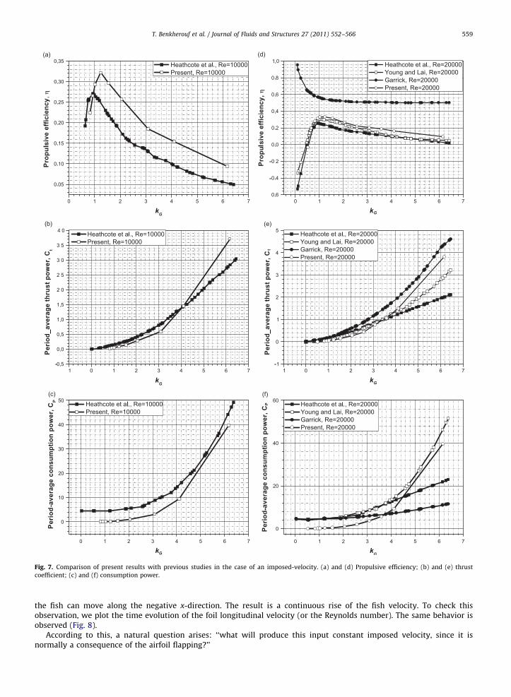
Fig. 7. Comparison of present results with previous studies in the case of an imposed-velocity. (a) and (d) Propulsive efficiency; (b) and (e) thrust

coefficient; (c) and (f) consumption power.


the fish can move along the negative x-direction. The result is a continuous rise of the fish velocity. To check thisobservation, we plot the time evolution of the foil longitudinal velocity (or the Reynolds number). The same behavior isobserved (Fig. 8).

According to this, a natural question arises: ‘‘what will produce this input constant imposed velocity, since it isnormally a consequence of the airfoil flapping?’’

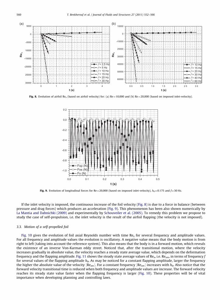
Fig. 8. Evolution of airfoil Rex (based on airfoil velocity) for: (a) Re¼10,000 and (b) Re¼20,000 (based on imposed inlet-velocity).

Fig. 9. Evolution of longitudinal forces for Re¼20,000 (based on imposed inlet-velocity), h0¼0.175 and f¼30 Hz.


If the inlet velocity is imposed, the continuous increase of the foil velocity (Fig. 8) is due to a force in balance (betweenpressure and drag forces) which produces an acceleration (Fig. 9). This phenomenon has been also shown numerically byLa Mantia and Dabnichki (2009) and experimentally by Schouveiler et al. (2005). To remedy this problem we propose tostudy the case of self-propulsion, i.e. the inlet velocity is the result of the airfoil flapping (the velocity is not imposed).

3.3. Motion of a self-propelled foil

Fig. 10 gives the evolution of foil axial Reynolds number with time Rex for several frequency and amplitude values.For all frequency and amplitude values the evolution is oscillatory. A negative value means that the body motion is fromright to left (taking into account the reference system). This also means that the body is in a forward motion, which revealsthe existence of an inverse Von-Karman eddy street. Noticed that, after the transitional motion, where the velocityincreases gradually in absolute value, the velocity reaches a steady state average value, which depends on the deformationfrequency and the flapping amplitude. Fig. 11 shows the steady state average values of Rex, i.e. Rexm, in terms of frequency f

for several values of the flapping amplitude h0. As may be noticed for a constant flapping amplitude, larger the frequencythe higher the absolute value of the velocity 9Rexm9. For a constant frequency 9Rexm9 increases with h0. Also notice that theforward velocity transitional time is reduced when both frequency and amplitude values are increase. The forward velocityreaches its steady state value faster when the flapping frequency is larger (Fig. 10). These properties will be of vitalimportance when developing planning and controlling laws.

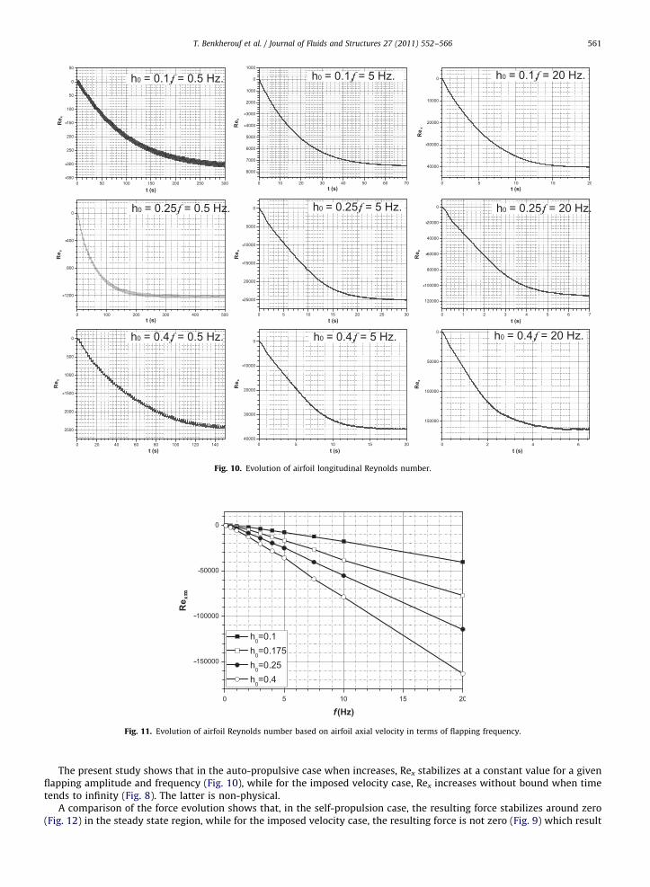
Fig. 10. Evolution of airfoil longitudinal Reynolds number.

Fig. 11. Evolution of airfoil Reynolds number based on airfoil axial velocity in terms of flapping frequency.


The present study shows that in the auto-propulsive case when increases, Rex stabilizes at a constant value for a givenflapping amplitude and frequency (Fig. 10), while for the imposed velocity case, Rex increases without bound when timetends to infinity (Fig. 8). The latter is non-physical.

A comparison of the force evolution shows that, in the self-propulsion case, the resulting force stabilizes around zero(Fig. 12) in the steady state region, while for the imposed velocity case, the resulting force is not zero (Fig. 9) which result

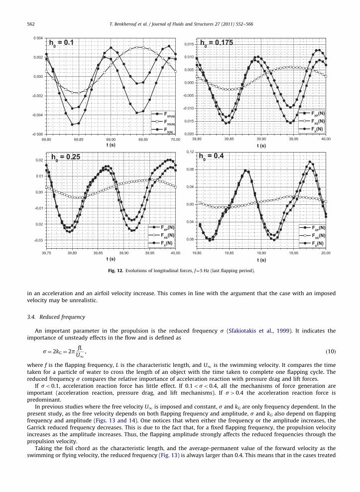
Fig. 12. Evolutions of longitudinal forces, f¼5 Hz (last flapping period).


in an acceleration and an airfoil velocity increase. This comes in line with the argument that the case with an imposedvelocity may be unrealistic.

3.4. Reduced frequency

An important parameter in the propulsion is the reduced frequency s (Sfakiotakis et al., 1999). It indicates theimportance of unsteady effects in the flow and is defined as

s¼ 2kG ¼ 2p fL

U1, ð10Þ

where f is the flapping frequency, L is the characteristic length, and U1 is the swimming velocity. It compares the timetaken for a particle of water to cross the length of an object with the time taken to complete one flapping cycle. Thereduced frequency s compares the relative importance of acceleration reaction with pressure drag and lift forces.

If so0.1, acceleration reaction force has little effect. If 0.1oso0.4, all the mechanisms of force generation areimportant (acceleration reaction, pressure drag, and lift mechanisms). If s40.4 the acceleration reaction force ispredominant.

In previous studies where the free velocity U1 is imposed and constant, s and kG are only frequency dependent. In thepresent study, as the free velocity depends on both flapping frequency and amplitude, s and kG also depend on flappingfrequency and amplitude (Figs. 13 and 14). One notices that when either the frequency or the amplitude increases, theGarrick reduced frequency decreases. This is due to the fact that, for a fixed flapping frequency, the propulsion velocityincreases as the amplitude increases. Thus, the flapping amplitude strongly affects the reduced frequencies through thepropulsion velocity.

Taking the foil chord as the characteristic length, and the average-permanent value of the forward velocity as theswimming or flying velocity, the reduced frequency (Fig. 13) is always larger than 0.4. This means that in the cases treated

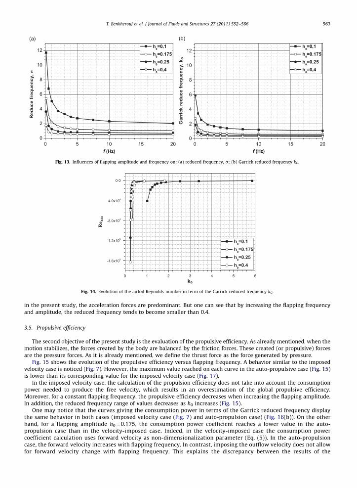
Fig. 13. Influences of flapping amplitude and frequency on: (a) reduced frequency, s; (b) Garrick reduced frequency kG.

Fig. 14. Evolution of the airfoil Reynolds number in term of the Garrick reduced frequency kG.


in the present study, the acceleration forces are predominant. But one can see that by increasing the flapping frequencyand amplitude, the reduced frequency tends to become smaller than 0.4.

3.5. Propulsive efficiency

The second objective of the present study is the evaluation of the propulsive efficiency. As already mentioned, when themotion stabilizes, the forces created by the body are balanced by the friction forces. These created (or propulsive) forcesare the pressure forces. As it is already mentioned, we define the thrust force as the force generated by pressure.

Fig. 15 shows the evolution of the propulsive efficiency versus flapping frequency. A behavior similar to the imposedvelocity case is noticed (Fig. 7). However, the maximum value reached on each curve in the auto-propulsive case (Fig. 15)is lower than its corresponding value for the imposed velocity case (Fig. 17).

In the imposed velocity case, the calculation of the propulsion efficiency does not take into account the consumptionpower needed to produce the free velocity, which results in an overestimation of the global propulsive efficiency.Moreover, for a constant flapping frequency, the propulsive efficiency decreases when increasing the flapping amplitude.In addition, the reduced frequency range of values decreases as h0 increases (Fig. 15).

One may notice that the curves giving the consumption power in terms of the Garrick reduced frequency displaythe same behavior in both cases (imposed velocity case (Fig. 7) and auto-propulsion case) (Fig. 16(b)). On the otherhand, for a flapping amplitude h0¼0.175, the consumption power coefficient reaches a lower value in the auto-propulsion case than in the velocity-imposed case. Indeed, in the velocity-imposed case the consumption powercoefficient calculation uses forward velocity as non-dimensionalization parameter (Eq. (5)). In the auto-propulsioncase, the forward velocity increases with flapping frequency. In contrast, imposing the outflow velocity does not allowfor forward velocity change with flapping frequency. This explains the discrepancy between the results of the

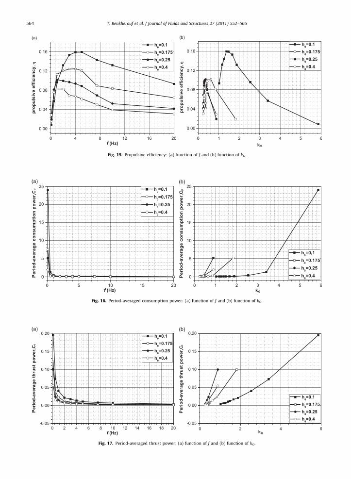
Fig. 15. Propulsive efficiency: (a) function of f and (b) function of kG.

Fig. 16. Period-averaged consumption power: (a) function of f and (b) function of kG.

Fig. 17. Period-averaged thrust power: (a) function of f and (b) function of kG.


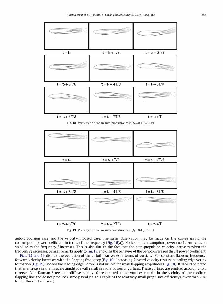
Fig. 18. Vorticity field for an auto-propulsive case (h0¼0.1, f¼5 Hz).

Fig. 19. Vorticity field for an auto-propulsive case (h0¼0.4, f¼5 Hz).


auto-propulsion case and the velocity-imposed case. The same observation may be made on the curves giving theconsumption power coefficient in terms of the frequency (Fig. 16(a)). Notice that consumption power coefficient tends tostabilize as the frequency f increases. This is also due to the fact that the auto-propulsion velocity increases when thefrequency f increases. Similar remarks apply to Fig. 17, showing the behavior of the period-averaged thrust power coefficient.

Figs. 18 and 19 display the evolution of the airfoil near wake in terms of vorticity. For constant flapping frequency,forward velocity increases with the flapping frequency (Fig. 10). Increasing forward velocity results in leading edge vortexformation (Fig. 19). Indeed the leading edge vortex is not visible for small flapping amplitudes (Fig. 18). It should be notedthat an increase in the flapping amplitude will result in more powerful vortices. These vortices are emitted according to areversed Von-Karman Street and diffuse rapidly. Once emitted, these vortices remain in the vicinity of the mediumflapping line and do not produce a strong axial jet. This explains the relatively small propulsive efficiency (lower than 20%,for all the studied cases).


4. Conclusion

An investigation of the flapping-fin propulsion is performed. Forward velocity and propulsive efficiency are computedwith homemade User Defined Functions hooked to Ansys-Fluent. We show that the proposed method can simulate theflow around a self-propelled body. In a first step the method is implemented under the same conditions as those used byvarious authors for validation purpose. The comparison results are satisfactory.

In a second step the self-propulsion case is considered. It is shown that, in this case, flapping produces a self-propulsion.In addition the propulsion velocity increases with both flapping frequency and amplitude. To each amplitude correspondsa frequency with maximum propulsive efficiency and minimum energy cost.

On the other hand a simple flapping does not produce a high propulsive efficiency. This is due to the fact that, eventhough the emitted vortices form a reversed Von-Karman Street, the vortices aligned with the medium flapping line and inits vicinity. As a result, the axial jet produced is not strong.

To remedy this problem two studies, on devoted to a combination between a flapping and a flexure motions and thesecond study devoted to a combination between a flapping and a rotation are in current development. We expect this tomove emitted vortices away from the vicinity of the medium flapping line and produce a more strong axial jet, thusincreasing the propulsive efficiency. A three dimensional simulation of the same configuration using an LES turbulentmodel is in current development.

References

Anderson, J.M., Streitlien, K., Barrett, D.S., Triantafyllou, M.S., 1998. Oscillating foils of high propulsive efficiency. Journal of Fluid Mechanics 360, 41–72.Bandyopadhyay, P.R., 2004. Biology-inspired science and technology for autonomous underwater vehicles. IEEE Journal of Oceanic Engineering 29,

542–546.Betz, A., 1912. Einbeitragzurerklarung des segelfluges. ZeitschriftfurFlugtechnik und Motorluftschiffahrt 3, 269–272.Fish, F.E., Lauder, G.V., 2006. Passive and active flow control by swimming fishes and mammals. Annual Review of Fluid Mechanics 38, 193–224.Fish, F.E., 2004. Structure and mechanics of non piscine control surfaces. IEEE Journal of Oceanic Engineering 29, 605–621.Freymuth, P., 1988. Propulsive vortical signature of plunging and pitching airfoils. American Institute of Aeronautics and Astronautics Journal 26,

881–883.Garrick, I.E., 1936. Propulsion of a flapping and oscillating airfoil. National Advisory Committee for Aeronautics, 567.Heathcote, S., Wang, Z., Gursul, I., 2008. Effect of spanwise flexibility on flapping wing propulsion. Journal of Fluids and Structures 24, 183–199.Hoa, S., Nassefa, H., Pornsinsirirakb, N., Taib, Y.C., Hoa, C.M., 2003. Unsteady aerodynamics and flow control for flapping wing flyers. Progress in Aerospace

Sciences 39, 635–681.Isogai, K., Shinmoto, Y., Watanabe, Y., 1999. Effect of dynamic stall on propulsive efficiency and thrust of a flapping airfoil. AIAA Journal 37, 1145–1151.Knoller, R., 1909. Die gesetze des luftwiderstands. Flug-und Motortechnik (Wien) 3, 1–7.La Mantia, M., Dabnichki, P., 2009. Unsteady panel method for flapping foil. Engineering Analysis with Boundary Elements 33, 572–580.Lauder, G.V., 2005. Locomotion. In: Evans, D.H., Claiborne, J.B. (Eds.), The Physiology of Fishes third ed., CRC, Boca Raton, pp. 3–46.Lauder, G.V., Drucker, E.G., 2004. Morphology and experimental hydrodynamics of fish fin control surfaces. IEEE Journal of Oceanic Engineering 29,

556–571.Leroyer, A., Visonneau, M., 2005. Numerical methods for RANSE simulations of a self-propelled fish-like body. Journal of Fluids and Structures 20,

975–991.Lin, C.S., Hwu, C., Young, W.B., 2006. The thrust and lift of an ornithopter’s membrane wings with simple flapping motion. Aerospace Science and

Technology 10, 111–119.Low, K.H., 2009. Modelling and parametric study of modular undulating fin rays for fish robots. Mechanism and Machine Theory 44, 615–632.Mazaheri, K., Ebrahimi, A., 2010. Experimental investigation of the effect of chordwise flexibility on the aerodynamics of flapping wings in hovering flight.

Journal of Fluids and Structures 26 (4), 544–558.Miao, J.M., Ho, M.H., 2006. Effect of flexure on aerodynamic propulsive efficiency of flapping flexible airfoil. Journal of Fluids and Structures 22, 401–419.Oshima, Y., Natsume, A., 1980. Flow field around an oscillating foil. In: Merzkirch, W. (Ed.), Flow Visualization II. Hemisphere. New York. pp. 295–299.Oshima, Y., Oshima, K., 1980. Vortical flow behind and oscillating foil. In: Proceedings of the 15th International Congress; International Union of

Theoretical and Applied Mechanics. Toronto. North-Holland. Amsterdam. pp. 357–368.Postlethwaite, C.M., Psemeneki, T.M., Selimkhanov, J., Silber, M., MacIver, M.A., 2008. Optimal movement in the prey strikes of weakly electric fish: a case

study of the interplay of body plan and movement capability. Journal of Royal Society. Interface doi:10.1098/rsif.2008.0286 Published online.Prangemeier, T., Rival, D., Tropea, C., 2010. The manipulation of trailing-edge vortices for an airfoil in plunging motion. Journal of Fluids and Structures 26,

193–204.Rhie, C.M., Chow, W.L., 1983. Numerical study of the turbulent flow past an airfoil with trailing edge separation. AIAA Journal 21 (11), 1525–1532.Rozhdestvensky, K.V., Ryzhov, V.A., 2003. Aerohydrodynamics of flapping-wing propulsors. Progress in Aerospace Sciences 39, 585–633.Schouveiler, I., Hover, F.S., Triantafyllou, M.S., 2005. Performance of flapping foil propulsion. Journal of fluids and structures 20 (7), 949–959.Sfakiotakis, M., Lane, D.M., Daviesand, J.B.C., 1999. Review of fish swimming modes for aquatic locomotion. IEEE Journal of Oceanic Engineering 24,

237–252.Sheu, T.W.H., Chen, Y.H., 2007. Numerical study of flow field induced by a locomotive fish in the moving meshes. International Journal of Numerical

Methods in Engineering 69, 2247–2263.Triantafyllou, M.S., Triantafyllou, G.S., Yue, D.K.P., 2000. Hydrodynamics of fish like swimming. Annual Review of Fluid Mechanics 32, 33–53.Triantafyllou, M.S., Techet, A.H., Hover, F.S., 2004. Review of experimental work in biomimetic foils. IEEE Journal of Oceanic Engineering 29, 585–594.Tuncer, I.H., Kaya, M., 2003. Thrust generation caused by flapping airfoils in a biplane configuration. Journal of Aircraft 40, 509–515.Van Leer, B., 1979. Toward the ultimate conservative difference scheme. IV. A second order sequel to Godunov’s method. Journal of Computational

Physics 32, 101–136.Webb, P.W., 1998. Swimming. In: Evans, D.H. (Ed.), The Physiology of Fishes 2nd edition CRC, Boca Raton, Florida, pp. 3–24.Wilga, C.D., Lauder, G.V., 2004. Biomechanics of locomotion in sharks, rays and chimeras. In: Carrier, J.C., Musick, J.A., Heithaus, M.R. (Eds.), Biology of

Sharks and Their Relatives. CRC, Boca Raton, pp. 139–164.Yu, J., Liu, L., Tan, M., 2008. Three-dimensional dynamic modeling of robotic fish: simulations and experiments. Transactions of the Institute of

Measurement and Control 30 (3/4), 239–2580, doi:10.1177/0142331208090045.Young, J., Lai, J.C.S., 2004. Oscillation frequency and amplitude effects on the wake of a plunging airfoil. AIAA Journal 42, 2042–2052.Yu, J., Hu, Y., Huo, J., Wang, L., 2009. Dolphin-like propulsive mechanism based on an adjustable Scotch yoke. Mechanism and Machine Theory 44,

603–614.

dx.doi.org/10.1098/rsif.2008.0286

dx.doi.org/10.1177/0142331208090045

Documents

Efficiency of an auto-propelled flapping airfoil