36 IEEE/ASME TRANSACTIONS ON MECHATRONICS, VOL. 17, NO. 1, FEBRUARY 2012

Modeling, Simulation, and Performance of aSynergistically Propelled Ichthyoid

Paul C. Strefling, Aren M. Hellum, and Ranjan Mukherjee, Senior Member, IEEE

Abstract—We have developed a novel type of submersible namedthe Synergistically Propelled Ichthyoid (SPI). The SPI is propelledby the synergistic combination of jet action and oscillatory motionof a fluttering fluid-conveying tail. Two dynamic models for an SPIare presented and solved: an analytically tractable model and amore complex model that captures the complete dynamics in twodimensions. The latter model has been solved numerically—thesesimulations show a benefit of using a fluttering tail relative to adimensionally identical rigid tail. Construction details of an exper-imental realization are provided, and preliminary measurementstaken using that platform are also provided. These measurementsqualitatively confirm the simulation’s conclusion that a flutteringflexible tail is capable of higher speed than a dimensionally identi-cal rigid tail.

Index Terms—Biomimetic, compliant mechanisms, computa-tional modeling, energy efficiency, fluid-conveying pipe, fluid flow,fluid jet, flutter instability, force, hydrodynamic model, hydro-dynamics, marine vehicles, mathematical model, mobile robots,propulsion, robotic fish, traveling wave.

I. INTRODUCTION

F ISH-LIKE propulsion has been a subject of academic in-terest since Gray’s pioneering work in the 1930s; the

oft-cited “Gray’s Paradox” is derived from [10] in which thespeed attained by a dolphin was calculated to require approxi-mately seven times the power available to the animal. Thoughlater workers resolved this apparent paradox (see the work byFish [9]), interest in the efficiency of fish-like motion has beensustained to the present day. An early model of oscillatorypropulsion proposed by Taylor [30] was based on calculation ofthe resistive force applied by the surrounding fluid; this model,which neglects inertial effects, is more appropriate to the studyof low-Reynolds number propulsion, such as that of spermato-zoa. These inertial effects were accounted for by Lighthill [17],which used slender-body theory to approximate the effect ofthe pressure field surrounding the fish. Lighthill found that atraveling waveform with higher amplitude at the tail than thehead is required to produce efficient thrust. Later works haveextended these initial efforts to account for a planform of vari-able height [33], deflections of arbitrary amplitude [19], and toaccount for the wing-like “lunate” tail, which is a feature of fastcarangiform swimmers [8].

Manuscript received April 1, 2011; revised July 28, 2011; accepted October7, 2011. Date of publication December 12, 2011; date of current version January9, 2012. Recommended by Guest Editor Y. Chen. This work was supported bythe Office of Naval Research under Grant N00014-08-1-0460 and by the Na-tional Science Foundation under Grant CMMI-1131170.

The authors are with the Department of Mechanical Engineering, Michi-gan State University, East Lansing, MI 48824 USA (e-mail: strefli3@msu.edu;aren.hellum@gmail.com; mukherji@egr.msu.edu).

Color versions of one or more of the figures in this paper are available onlineat http://ieeexplore.ieee.org.

Digital Object Identifier 10.1109/TMECH.2011.2172950

It is difficult to precisely measure the efficiency of a self-propelled swimming body, since the sources of drag and thrustcannot be separated; a variety of approaches [28] have beenemployed to determine these. Lighthill’s slender body methodsestimate that 90% of the power expended by a swimming fish isavailable to propel the fish, and that the remainder is wasted, askinetic energy in the wake. This value of 90% Froude efficiencylines up well with a figure of 87% found by Anderson et al.[2] on a simplified experimental setup. The temptation amongresearchers to “chase the tail” is driven in large part by theseimpressive efficiency figures.

The predicted efficiency of fish locomotion has motivated thedevelopment of many fish-like robotic platforms. A well-knownbiomimetic platform is MIT’s RoboTuna [4], [31], which usesan articulated tail covered by a flexible sheath. The links whichmake up this tail are individually actuated in an approximation ofa fishes motion. A different type of articulated system was builtby McMasters et al. [21], which used a novel geared mechanismto produce a fish-like motion using only a single servomotor.Yu et al. [34] constructed an articulated system and designedtail motion for three types of turning behaviors. Morgansen etal. [22] also built an articulated system and achieved controlusing wing-like pectoral fins. Saimek and Li [27] designed atwo-link pitching tail and used a motor at the base of the first linkto achieve heave and pitch motion. A mathematical descriptionof the thrust generated can be found in the work by Kansoet al. [16] which is unique in that it investigates the thrustproduced by an articulated system rather than that produced by acontinuous waveform, as developed by Lighthill [17]–[19]. Thework on articulated systems has not been confined to traditionalservomotor transmissions; Chen et al. [7] and Guo et al. [11]used electrically active polymers for actuation.

An alternate approach to articulated systems was taken byAlvarado and Youcef-Toumi [1], who described a system whichused a flexible tail, excited with a single actuator at the base.The advantage of the latter approach is that a flexible tail canbe oscillated near its natural frequency; in contrast, the naturaldynamics of an articulated tail impede the actuators’ ability tocreate the desired waveform. Thus, a submersible constructedwith a flexible tail is likely to have reduced transmission lossesand lower motor bandwidth requirements.

The flexible tail mechanism described in this paper is notactuated by an actuator at the base but instead by flutter insta-bility induced by conveying fluid through a central tube. Theresulting propulsor creates thrust by means of both the jet mo-mentum and the fluttering action of the tail. We have coined theterm “Synergistically Propelled Ichthyoid” (SPI) to describevehicles using this type of propulsion mechanism. An earlier

1083-4435/$26.00 © 2011 IEEE

STREFLING et al.: MODELING, SIMULATION, AND PERFORMANCE OF A SYNERGISTICALLY PROPELLED ICHTHYOID 37

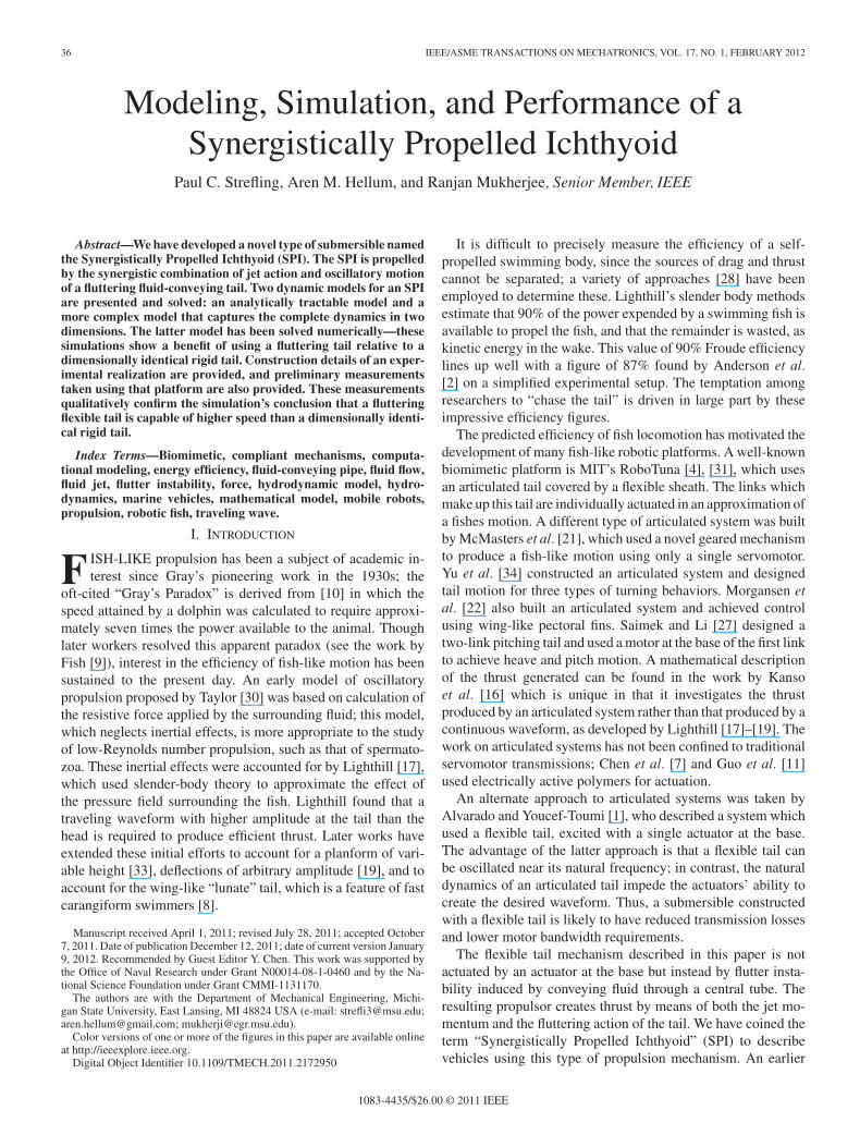
Fig. 1. Simplified view of the SPI, which is comprised of a rigid head andflexible fluid-conveying tail.

attempt to design this type of propulsor was made by Paidoussiset al. in the mid-1970s [23], although it was placed on a largesurface vessel, rather than the small submersible described inthis study. In addition to the aforementioned paper by Alvaradoand Youcef-Toumi, Harper et al. [12] constructed an articulatedtail that was actuated in series with lateral and torsional springsso that the motion of the tail is underactuated; this system repre-sents an intermediate form between flexible tails and articulatedsystems. Recently, Aureli et al. [3] and Liu et al. [20] have con-structed flexible-tailed systems actuated by ionic polymer–metalcomposite and slider–crank mechanism, respectively. Suzumoriet al. [29] developed flexible pneumatic actuators that can beadapted to a tail-like propulsor.

This paper is structured as follows. A description of a sim-plified, analytically tractable model of an SPI is presented inSection II. A more general model is presented in Section III.The numerical solutions of those more complicated expressionsare presented in Section IV. We have also constructed an ex-perimental platform; construction details and preliminary mea-surements taken with that platform are presented in Section V.Concluding remarks and description of future work are given inSection VI.

II. BACKGROUND

The SPI uses as its propulsor a fluid-conveying tail that oscil-lates due to flutter instability. Earlier experimental work doneon this type of propulsor [23], [24] showed that such a systemproduces positive thrust if the phase velocity of the tail displace-ment was greater than the forward speed of the vessel, a resultthat confirms Lighthill’s [17] theoretical developments.

The neutrally buoyant hull proposed here is much smallerthan the surface hull built by Paidoussis; this seemingly trivialvariation means that the tail’s motion is coupled to the accel-erations of the hull. A linearized version of this analysis wasperformed by Hellum et al. [14], who determined the stability ofa fluid-conveying, fluid-immersed pipe affixed to a rigid body.The system proposed in that work is assumed to be travelingwith constant forward velocity through the immersing medium,but transverse acceleration and small rotations of the rigid bodyare permitted. The system analyzed in that work is presented inFig. 1.

The equation of motion for a fluid-conveying, fluid-immersedpipe is given by [14]

Y ′′′′ + (u2i + u2

e )Y′′ + 2(ui

√βi + ue

√βe)Y + Y = 0 (1)

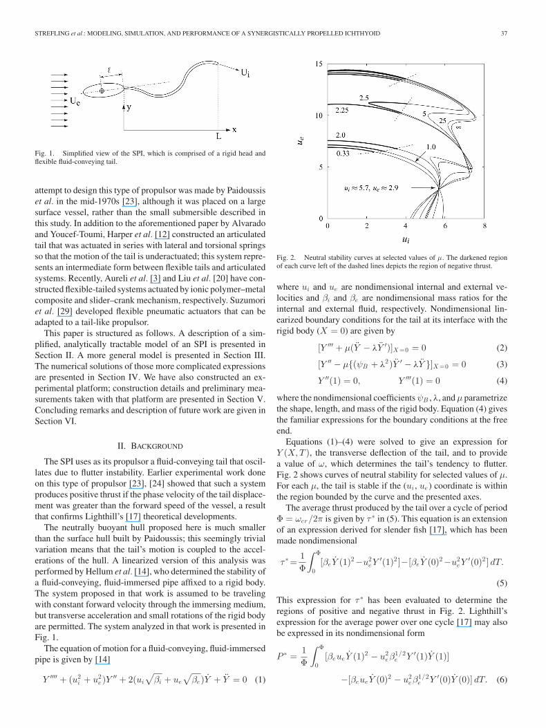
Fig. 2. Neutral stability curves at selected values of μ. The darkened regionof each curve left of the dashed lines depicts the region of negative thrust.

where ui and ue are nondimensional internal and external ve-locities and βi and βe are nondimensional mass ratios for theinternal and external fluid, respectively. Nondimensional lin-earized boundary conditions for the tail at its interface with therigid body (X = 0) are given by

[Y ′′′ + μ(Y − λY ′)]X =0 = 0 (2)

[Y ′′ − μ{(ψB + λ2)Y ′ − λY }]X =0 = 0 (3)

Y ′′(1) = 0, Y ′′′(1) = 0 (4)

where the nondimensional coefficients ψB , λ, and μ parametrizethe shape, length, and mass of the rigid body. Equation (4) givesthe familiar expressions for the boundary conditions at the freeend.

Equations (1)–(4) were solved to give an expression forY (X,T ), the transverse deflection of the tail, and to providea value of ω, which determines the tail’s tendency to flutter.Fig. 2 shows curves of neutral stability for selected values of μ.For each μ, the tail is stable if the (ui , ue ) coordinate is withinthe region bounded by the curve and the presented axes.

The average thrust produced by the tail over a cycle of periodΦ = ωcr/2π is given by τ ∗ in (5). This equation is an extensionof an expression derived for slender fish [17], which has beenmade nondimensional

τ ∗=1Φ

∫ Φ

0[βeY (1)2−u2

eY′(1)2 ]−[βeY (0)2−u2

eY′(0)2 ] dT.

(5)

This expression for τ ∗ has been evaluated to determine theregions of positive and negative thrust in Fig. 2. Lighthill’sexpression for the average power over one cycle [17] may alsobe expressed in its nondimensional form

P ∗ =1Φ

∫ Φ

0[βeueY (1)2 − u2

eβ1/2e Y ′(1)Y (1)]

−[βeueY (0)2 − u2eβ

1/2e Y ′(0)Y (0)] dT. (6)

38 IEEE/ASME TRANSACTIONS ON MECHATRONICS, VOL. 17, NO. 1, FEBRUARY 2012

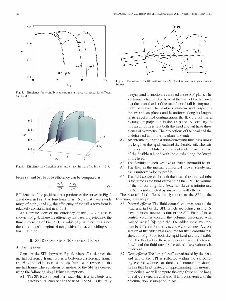
Fig. 3. Efficiency for neutrally stable points in the ui -ue space, for differentvalues of μ.

Fig. 4. Efficiency as a function of ui and ue for the mass fraction μ = 2.5.

From (5) and (6), Froude efficiency can be computed as

η =τUe

P=

τ ∗ue

P ∗ . (7)

Efficiencies of the positive thrust portions of the curves in Fig. 2are shown in Fig. 3 as functions of ue . Note that over a widerange of both μ and ue , the efficiency of the tail’s waveform isrelatively constant, and near 50%.

An alternate view of the efficiency of the μ = 2.5 case isshown in Fig. 4, where the efficiency has been projected into thethird dimension of Fig. 2. This value of μ is interesting sincethere is an interim region of nonpositive thrust, coinciding withlow ui at high ue .

III. SPI DYNAMICS IN A NONINERTIAL FRAME

A. Assumptions

Consider the SPI shown in Fig. 5, where XY denotes theinertial reference frame, xy is a body-fixed reference frame,and θ is the orientation of the xy frame with respect to theinertial frame. The equations of motion of the SPI are derivedusing the following simplifying assumptions.

A1. The SPI is comprised of a head, which is a rigid body, anda flexible tail clamped to the head. The SPI is neutrally

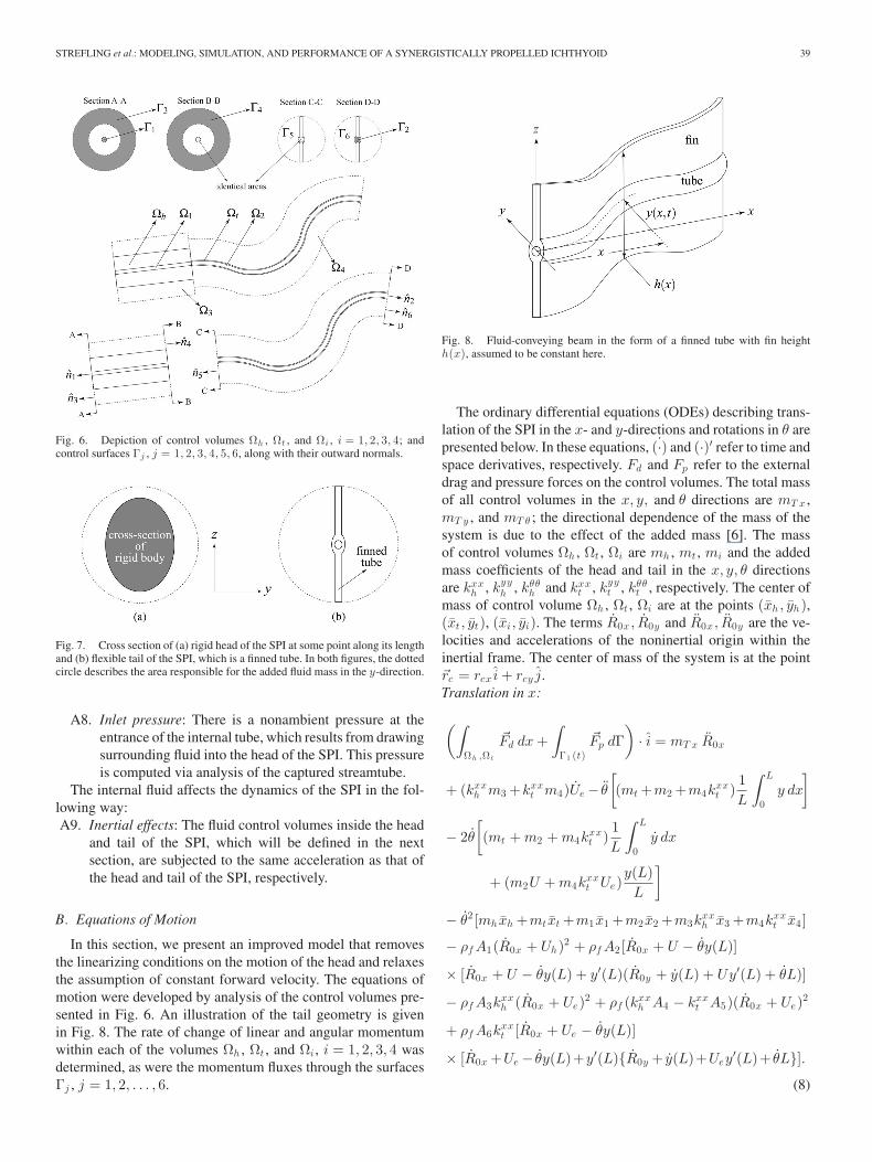
Fig. 5. Depiction of the SPI with inertial (XY ) and noninertial (xy) referenceframes.

buoyant and its motion is confined to the XY plane. Thexy frame is fixed to the head at the base of the tail suchthat the neutral axis of the undeformed tail is congruentwith the x-axis. The head is symmetric with respect tothe xz and xy planes and is uniform along its length.In its undeformed configuration, the flexible tail has arectangular projection in the xz plane. A corollary tothis assumption is that both the head and tail have threeplanes of symmetry. The projections of the head and theundeformed tail in the xy plane is slender.

A2. An internal cylindrical fluid-conveying tube runs alongthe length of the rigid head and the flexible tail. The axisof the cylindrical tube is congruent with the neutral axisof the flexible tail and with the x-axis along the lengthof the head.

A3. The flexible tail behaves like an Euler–Bernoulli beam.A4. The flow in the internal cylindrical tube is steady and

has a uniform velocity profile.A5. The fluid conveyed through the internal cylindrical tube

is the same as the fluid surrounding the SPI. The volumeof the surrounding fluid (external fluid) is infinite andthe SPI is not affected by surface or wall effects.

The external fluid affects the dynamics of the SPI in thefollowing three ways:

A6. Inertial effects: The fluid control volumes around thehead and tail of the SPI, which are defined in Fig. 6,have identical motion as that of the SPI. Each of thesecontrol volumes contain the volumes associated with“added mass” [6]; note that the added-mass volumesmay be different for the x, y, and θ coordinates. A crosssection of the added mass volume for the y coordinate isshown in Fig. 7 for both the rigid head and the flexibletail. The fluid within these volumes is inviscid (potentialflow), and the fluid outside the added mass volumes isquiescent.

A7. Drag effects: The “drag force” experienced by the headand tail of the SPI is reflected within the surround-ing control volumes of fluid as a momentum deficitwithin that fluid. Instead of approximating this momen-tum deficit, we will compute the drag force on the bodydirectly, via separate analysis. This is consistent with thepotential flow assumption in A6.

STREFLING et al.: MODELING, SIMULATION, AND PERFORMANCE OF A SYNERGISTICALLY PROPELLED ICHTHYOID 39

Fig. 6. Depiction of control volumes Ωh , Ωt , and Ωi , i = 1, 2, 3, 4; andcontrol surfaces Γj , j = 1, 2, 3, 4, 5, 6, along with their outward normals.

Fig. 7. Cross section of (a) rigid head of the SPI at some point along its lengthand (b) flexible tail of the SPI, which is a finned tube. In both figures, the dottedcircle describes the area responsible for the added fluid mass in the y-direction.

A8. Inlet pressure: There is a nonambient pressure at theentrance of the internal tube, which results from drawingsurrounding fluid into the head of the SPI. This pressureis computed via analysis of the captured streamtube.

The internal fluid affects the dynamics of the SPI in the fol-lowing way:A9. Inertial effects: The fluid control volumes inside the head

and tail of the SPI, which will be defined in the nextsection, are subjected to the same acceleration as that ofthe head and tail of the SPI, respectively.

B. Equations of Motion

In this section, we present an improved model that removesthe linearizing conditions on the motion of the head and relaxesthe assumption of constant forward velocity. The equations ofmotion were developed by analysis of the control volumes pre-sented in Fig. 6. An illustration of the tail geometry is givenin Fig. 8. The rate of change of linear and angular momentumwithin each of the volumes Ωh , Ωt , and Ωi , i = 1, 2, 3, 4 wasdetermined, as were the momentum fluxes through the surfacesΓj , j = 1, 2, . . . , 6.

Fig. 8. Fluid-conveying beam in the form of a finned tube with fin heighth(x), assumed to be constant here.

The ordinary differential equations (ODEs) describing trans-lation of the SPI in the x- and y-directions and rotations in θ arepresented below. In these equations, ˙(·) and (·)′ refer to time andspace derivatives, respectively. Fd and Fp refer to the externaldrag and pressure forces on the control volumes. The total massof all control volumes in the x, y, and θ directions are mT x ,mT y , and mT θ ; the directional dependence of the mass of thesystem is due to the effect of the added mass [6]. The massof control volumes Ωh , Ωt , Ωi are mh , mt , mi and the addedmass coefficients of the head and tail in the x, y, θ directionsare kxx

h , kyyh , kθθ

h and kxxt , kyy

t , kθθt , respectively. The center of

mass of control volume Ωh , Ωt , Ωi are at the points (xh , yh),(xt , yt), (xi , yi). The terms R0x , R0y and R0x , R0y are the ve-locities and accelerations of the noninertial origin within theinertial frame. The center of mass of the system is at the pointrc = rcx i + rcy j.Translation in x:

(∫

Ωh ,Ω t

Fd dx +∫

Γ1 (t)

Fp dΓ)· i = mT x R0x

+ (kxxh m3 +kxx

t m4)Ue − θ

[(mt +m2 +m4k

xxt )

1L

∫ L

0y dx

]

− 2θ

[(mt + m2 + m4k

xxt )

1L

∫ L

0y dx

+ (m2U + m4kxxt Ue)

y(L)L

]

− θ2 [mhxh +mtxt +m1 x1 +m2 x2 +m3kxxh x3 +m4k

xxt x4 ]

− ρf A1(R0x + Uh)2 + ρf A2 [R0x + U − θy(L)]

× [R0x + U − θy(L) + y′(L)(R0y + y(L) + Uy′(L) + θL)]

− ρf A3kxxh (R0x + Ue)2 + ρf (kxx

h A4 − kxxt A5)(R0x + Ue)2

+ ρf A6kxxt [R0x + Ue − θy(L)]

× [R0x +Ue − θy(L)+y′(L){R0y + y(L)+Uey′(L)+ θL}].

(8)

40 IEEE/ASME TRANSACTIONS ON MECHATRONICS, VOL. 17, NO. 1, FEBRUARY 2012

Translation in y:

(∫

Ωh ,Ω t

Fd dx +∫

Γ1 (t)

Fp dΓ)· j = mT y R0y

+mt + m2 + m4k

yyt

L

∫ L

0y dx +

m2

L

∫ L

0(2Uy′ + U 2y′′) dx

+m4k

yyt

L

∫ L

0(2Uey

′ + U 2e y′′ + Uey

′) dx + θ[mhxh + mtxt

+ m1 x1 +m2 x2 +m3kyyh x3 +m4k

yyt x4 ]+2θ[m1Uh +m2U

+ (m3kyyh + m4k

yyt )Ue ] − θ2

[mt + m2 + m4k

xxt

L

∫ L

0ydx

]

+ ρf {A1 [R0y − θLh ][−R0x −Uh ]+A2 [R0y + y(L)+Uy′(L)

+ θL][R0x +U − θy(L)+y′(L)(R0y + y(L)+Uy′(L)+ θL)]

+ A3kyyh (R0y − θLh)[−R0x − Ue ] + (kyy

h A4 − kyyt A5)

×R0y [R0x +Ue ]+A6kyyt [R0y + θL+ y(L)+Uey

′(L)][R0x

+ Ue − θy(L) + y′(L){R0y + y(L) + Uey′(L) + θL}]}. (9)

Rotation in θ:∫

Ωh ,Ω t

(r − rc) × Fd dx +∫

Γ1 (t)(r − rc) × Fp dΓ

=mt

L

∫ L

0(x − rcx)y dx +

m2

L

∫ L

0(x − rcx)(y + 2Uy′

+ U 2y′′) dx +m4k

θθt

L

∫ L

0(x − rcx)(y + 2Uey

′ + U 2e y′′

+ Uey′) dx + Ue

[m3k

θθh rcy − m4k

θθt

1L

∫ L

0(y − rcy ) dx

]

+ θ

{Jzh + (m1 + m3k

θθh )

L2h

3+ (mt + m2 + m4k

θθt )

×[L2

3+

1L

∫ L

0y2 dx

]− [mhx2

h + mtx2t + m1 x

21 + m2 x

22

+ m3kθθh x2

3 + m4kθθt x2

4 ] −mt + m2 + m4k

θθt

L2

[∫ L

0y dx

]2}

+ 2θ

[(m1Uh + m3k

θθh Ue)

1Lh

∫ 0

−Lh

(x − rcx) dx

+ (m2U + m4kθθt Ue)

1L

∫ L

0(x − rcx) dx +

∫ L

0(y − rcy )

×(mt + m2 + m4k

θθt

Ly + (m2U + m4Uek

θθt )y′

)dx

]

+ ρf A1 [(−Lh − rcx)R0y + rcy (R0x +Uh)+ θ(L2h +Lhrcx)]

× [−R0x − Uh ] + ρf A2 [(L − rcx){R0y + y(L) + Uy′ + θL}

− {y(L) − rcy}{R0x + U − θy(L)} + θ{L2 + y2(L) − Lrcx

− y(L)rcy}][{R0x + U − θy(L)} + y′(L){R0y + y(L)

+ Uy′(L) + θL}] + ρf A3kθθh ({−Lh − rcx}R0y + rcy{R0x

+ Ue}+ θ{L2h +Lhrcx})[−R0x−Ue ]+ρf (A4k

θθh −A5k

θθt )

× (−rcxR0y + rcy{R0x + Ue})[R0x + Ue ] + ρf A6kθθt

× [(L − rcx){R0y + y(L) + θL + Uey′(L)} − {y(L) − rcy}

×{R0x +Ue − θy(L)}+ θ{L2 + y(L)2 − Lrcx − y(L)rcy}]

×[R0x +Ue − θy(L)+ y′(L){R0y + y(L)+ θL+Uey′(L)}].

(10)

Flexible Tail Equations:Equation (11) describes the motion of the flexible tail y(x, t),

which appears in (8)–(10):

EI∂4y

∂x4 +[m2

LU 2 +

m4kyyt

LU 2

e − Dbt

+∫ L

x

(mt + m2 + m4k

xxt

Lax +

m4kxxt

LUe − Dx

t

)dx

]∂2y

∂x2

+ 2[m2

LU +

m4kyyt

LUe

]∂2y

∂x∂t

+[−mt + m2 + m4k

xxt

Lax − m4(kxx

t − kyyt )

LUe + Dx

t

]∂y

∂x

+mt + m2 + m4k

yyt

L

(∂2y

∂t2+ ay

)− Dy

t = 0

(11)

where ax and ay are composed of the accelerations of the non-inertial frame in the x- and y-directions:

ax = R0x − θy − 2θ

[y +

m2U + m4kxxt Ue

mt + m2 + m4kxxt

y′]− θ2x

(12)

ay = R0y + θx + 2θ

[m2U + m4k

yyt Ue

mt + m2 + m4kyyt

]− θ2y. (13)

Since the noninertial reference frame is fixed at the base ofthe tail, the boundary conditions for the flexible tail are those ofa cantilever:

y(0) = 0, y′(0) = 0, y′′(L) = 0, y′′′(L) = 0.

External Forces:The external forces acting on the system are the pressure and

drag forces Fp and Fd . The pressure force acting at the inlet iscomputed by the analysis of a captured quasi-steady streamtube:

∫

Γ1 (t)

Fp dΓ = −A1ρf Uh(Uh − Ue) i.

The drag terms Dxt and Dy

t are given by

Dxt = DT

t − DNt y′

Dyt = DN

t + DTt y′

STREFLING et al.: MODELING, SIMULATION, AND PERFORMANCE OF A SYNERGISTICALLY PROPELLED ICHTHYOID 41

where DTt and DN

t are the drag forces on the tail in the tangentialand normal directions

DNt = −ρf hCN

t V Tt V N

t + ctVNt (14)

DTt = −ρf PtC

Tt V T

t |V Tt |. (15)

In the aforementioned expressions, h is the total tail height (seeFig. 8), and Pt is the cross-sectional perimeter of the tail. In (14)and (15), the coefficients CN

t and CTt are normal and tangen-

tial drag coefficients for the tail, which are analogous to thoseproposed by Taylor [30]. The additional viscous coefficients ct

and ch were added by later workers (see discussion in [25]) toaccount for the damping experienced by a flexible member im-mersed in quiescent fluid, i.e., Ue = 0. Taylor’s model also didnot consider the drag at the blunt trailing end of a slender bodysince that work considered the case of infinitely long slendermembers, following Relf and Powell [26]. This base drag Db

t isgiven by

Dbt = −1

2ρf AtC

bt

[V T

t

∣∣V Tt

∣∣]x=L

(16)

where the factor of 12 is a convention, based on the equation’s

similarity to the standard expression for the drag on a rigidbody. In the preceding expressions, the velocities V T

t and V Nt

represent the velocity of the fluid surrounding the tail in thetangential and normal directions:

V Tt = R0x − θy + (R0y + y + θx)y′

V Nt = R0y + y + θx − (R0x − θy)y′.

Similar expressions for the drag on the rigid head of the SPI aregiven as follows:

Dxh = −ρf Ph [CT

h R0x |R0x |] (17)

Dyh = −ρf Ph [CN

h R0x(R0y + θx) + ch(R0y + θx)] (18)

Dbh = −ρf

2Ah [Cb

hR0x |R0x |]x=0 (19)

where Ph is the perimeter of the head, Ah is the cross-sectionalarea of the head, and CN

h , CTh , and Cb

h are normal, tangential,and base drag coefficients for the head.

The i and j components of Fd in (8), (9) can now be expressedas follows:

∫

Ωh ,Ω t

Fd dx · i =∫

Ωh

DxhdΩ +

∫

Ω t

Dxt dΩ + Db

h

∫

Ωh ,Ω t

Fd dx · j =∫

Ωh

DyhdΩ +

∫

Ω t

Dyt dΩ + Db

h

∂y

∂x.

A detailed derivation of the equations in this section can befound in [13].

IV. SIMULATIONS

A. Numerical Methods and Parameters

The equations in the previous section were discretized us-ing a finite-difference scheme, converted to a set of first-orderODE’s and solved using a fourth-order Runge–Kutta integra-tor. A five-point stencil was used to approximate the required

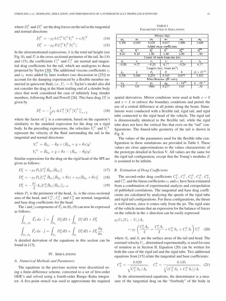
TABLE IPARAMETERS USED IN SIMULATIONS

spatial derivatives. Mirror conditions were used at both x = 0and x = L to enforce the boundary conditions and permit theuse of a central difference at all points along the beam. Simu-lations were conducted with a flexible tail, rigid tail, and rigidtube connected to the rigid head of the vehicle. The rigid tailis dimensionally identical to the flexible tail, while the rigidtube does not have the vertical fins that exist on the “tail” con-figurations. The finned-tube geometry of the tail is shown inFig. 8.

The values of the parameters used for the flexible tube con-figuration in these simulations are provided in Table I. Thesevalues are close approximations to the values characteristic ofthe prototype detailed in Section V. All values are the same forthe rigid tail configuration, except that the Young’s modulus Eis assumed to be infinite.

B. Estimation of Drag Coefficients

The second-order drag coefficients CTh , CT

t , CNh , CN

h , Cbh ,

and Cbt , and the linear coefficients ch and ct have been estimated

from a combination of experimental analysis and extrapolationof published correlations. The tangential and base drag coeffi-cients are calculated by analyzing the speeds of the rigid tubeand rigid tail configurations. For these configurations, the thrustis well known, since it comes only from the jet. The rigid stateof the vehicle means that an expression for the balance of forceson the vehicle in the x-direction can be easily expressed

ρf Uh(Uh − Ue)A1

= ρf

(Cb

hAh

2+

Cbt At

2+ CT

h Sh + CTt St

)U 2

e (20)

where Sh and St are the surface areas of the tail and head. Theexternal velocity Ue , determined experimentally, is used for easeof notation as in Section II. Equation (20) can be written forboth the case of the rigid tail and the rigid tube. Two additionalequations from [15] relate the tangential and base coefficients:

Cbh =

0.029√

CTh Sh/Ah

, Cbt =

0.1353

√(CT

h Sh + CTt St)/At

. (21)

In the aforementioned equations, the denominator is a mea-sure of the tangential drag on the “forebody” of the body in

42 IEEE/ASME TRANSACTIONS ON MECHATRONICS, VOL. 17, NO. 1, FEBRUARY 2012

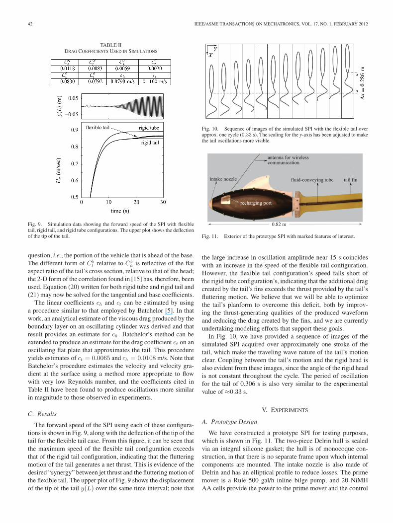
TABLE IIDRAG COEFFICIENTS USED IN SIMULATIONS

Fig. 9. Simulation data showing the forward speed of the SPI with flexibletail, rigid tail, and rigid tube configurations. The upper plot shows the deflectionof the tip of the tail.

question, i.e., the portion of the vehicle that is ahead of the base.The different form of Cb

t relative to Cbh is reflective of the flat

aspect ratio of the tail’s cross section, relative to that of the head;the 2-D form of the correlation found in [15] has, therefore, beenused. Equation (20) written for both rigid tube and rigid tail and(21) may now be solved for the tangential and base coefficients.

The linear coefficients ch and ct can be estimated by usinga procedure similar to that employed by Batchelor [5]. In thatwork, an analytical estimate of the viscous drag produced by theboundary layer on an oscillating cylinder was derived and thatresult provides an estimate for ch . Batchelor’s method can beextended to produce an estimate for the drag coefficient ct on anoscillating flat plate that approximates the tail. This procedureyields estimates of ct = 0.0065 and ch = 0.0108 m/s. Note thatBatchelor’s procedure estimates the velocity and velocity gra-dient at the surface using a method more appropriate to flowwith very low Reynolds number, and the coefficients cited inTable II have been found to produce oscillations more similarin magnitude to those observed in experiments.

C. Results

The forward speed of the SPI using each of these configura-tions is shown in Fig. 9, along with the deflection of the tip of thetail for the flexible tail case. From this figure, it can be seen thatthe maximum speed of the flexible tail configuration exceedsthat of the rigid tail configuration, indicating that the flutteringmotion of the tail generates a net thrust. This is evidence of thedesired “synergy” between jet thrust and the fluttering motion ofthe flexible tail. The upper plot of Fig. 9 shows the displacementof the tip of the tail y(L) over the same time interval; note that

Fig. 10. Sequence of images of the simulated SPI with the flexible tail overapprox. one cycle (0.33 s). The scaling for the y-axis has been adjusted to makethe tail oscillations more visible.

Fig. 11. Exterior of the prototype SPI with marked features of interest.

the large increase in oscillation amplitude near 15 s coincideswith an increase in the speed of the flexible tail configuration.However, the flexible tail configuration’s speed falls short ofthe rigid tube configuration’s, indicating that the additional dragcreated by the tail’s fins exceeds the thrust provided by the tail’sfluttering motion. We believe that we will be able to optimizethe tail’s planform to overcome this deficit, both by improv-ing the thrust-generating qualities of the produced waveformand reducing the drag created by the fins, and we are currentlyundertaking modeling efforts that support these goals.

In Fig. 10, we have provided a sequence of images of thesimulated SPI acquired over approximately one stroke of thetail, which make the traveling wave nature of the tail’s motionclear. Coupling between the tail’s motion and the rigid head isalso evident from these images, since the angle of the rigid headis not constant throughout the cycle. The period of oscillationfor the tail of 0.306 s is also very similar to the experimentalvalue of ≈0.33 s.

V. EXPERIMENTS

A. Prototype Design

We have constructed a prototype SPI for testing purposes,which is shown in Fig. 11. The two-piece Delrin hull is sealedvia an integral silicone gasket; the hull is of monocoque con-struction, in that there is no separate frame upon which internalcomponents are mounted. The intake nozzle is also made ofDelrin and has an elliptical profile to reduce losses. The primemover is a Rule 500 gal/h inline bilge pump, and 20 NiMHAA cells provide the power to the prime mover and the control

STREFLING et al.: MODELING, SIMULATION, AND PERFORMANCE OF A SYNERGISTICALLY PROPELLED ICHTHYOID 43

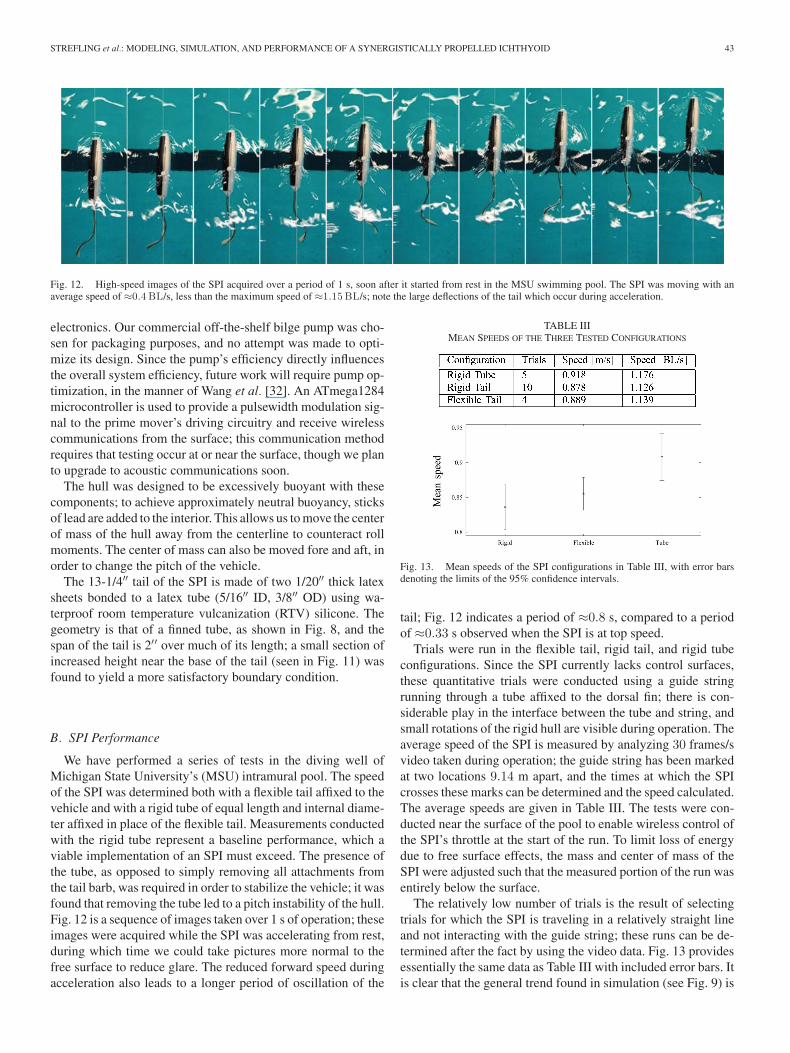
Fig. 12. High-speed images of the SPI acquired over a period of 1 s, soon after it started from rest in the MSU swimming pool. The SPI was moving with anaverage speed of ≈0.4 BL/s, less than the maximum speed of ≈1.15 BL/s; note the large deflections of the tail which occur during acceleration.

electronics. Our commercial off-the-shelf bilge pump was cho-sen for packaging purposes, and no attempt was made to opti-mize its design. Since the pump’s efficiency directly influencesthe overall system efficiency, future work will require pump op-timization, in the manner of Wang et al. [32]. An ATmega1284microcontroller is used to provide a pulsewidth modulation sig-nal to the prime mover’s driving circuitry and receive wirelesscommunications from the surface; this communication methodrequires that testing occur at or near the surface, though we planto upgrade to acoustic communications soon.

The hull was designed to be excessively buoyant with thesecomponents; to achieve approximately neutral buoyancy, sticksof lead are added to the interior. This allows us to move the centerof mass of the hull away from the centerline to counteract rollmoments. The center of mass can also be moved fore and aft, inorder to change the pitch of the vehicle.

The 13-1/4′′ tail of the SPI is made of two 1/20′′ thick latexsheets bonded to a latex tube (5/16′′ ID, 3/8′′ OD) using wa-terproof room temperature vulcanization (RTV) silicone. Thegeometry is that of a finned tube, as shown in Fig. 8, and thespan of the tail is 2′′ over much of its length; a small section ofincreased height near the base of the tail (seen in Fig. 11) wasfound to yield a more satisfactory boundary condition.

B. SPI Performance

We have performed a series of tests in the diving well ofMichigan State University’s (MSU) intramural pool. The speedof the SPI was determined both with a flexible tail affixed to thevehicle and with a rigid tube of equal length and internal diame-ter affixed in place of the flexible tail. Measurements conductedwith the rigid tube represent a baseline performance, which aviable implementation of an SPI must exceed. The presence ofthe tube, as opposed to simply removing all attachments fromthe tail barb, was required in order to stabilize the vehicle; it wasfound that removing the tube led to a pitch instability of the hull.Fig. 12 is a sequence of images taken over 1 s of operation; theseimages were acquired while the SPI was accelerating from rest,during which time we could take pictures more normal to thefree surface to reduce glare. The reduced forward speed duringacceleration also leads to a longer period of oscillation of the

TABLE IIIMEAN SPEEDS OF THE THREE TESTED CONFIGURATIONS

Fig. 13. Mean speeds of the SPI configurations in Table III, with error barsdenoting the limits of the 95% confidence intervals.

tail; Fig. 12 indicates a period of ≈0.8 s, compared to a periodof ≈0.33 s observed when the SPI is at top speed.

Trials were run in the flexible tail, rigid tail, and rigid tubeconfigurations. Since the SPI currently lacks control surfaces,these quantitative trials were conducted using a guide stringrunning through a tube affixed to the dorsal fin; there is con-siderable play in the interface between the tube and string, andsmall rotations of the rigid hull are visible during operation. Theaverage speed of the SPI is measured by analyzing 30 frames/svideo taken during operation; the guide string has been markedat two locations 9.14 m apart, and the times at which the SPIcrosses these marks can be determined and the speed calculated.The average speeds are given in Table III. The tests were con-ducted near the surface of the pool to enable wireless control ofthe SPI’s throttle at the start of the run. To limit loss of energydue to free surface effects, the mass and center of mass of theSPI were adjusted such that the measured portion of the run wasentirely below the surface.

The relatively low number of trials is the result of selectingtrials for which the SPI is traveling in a relatively straight lineand not interacting with the guide string; these runs can be de-termined after the fact by using the video data. Fig. 13 providesessentially the same data as Table III with included error bars. Itis clear that the general trend found in simulation (see Fig. 9) is

44 IEEE/ASME TRANSACTIONS ON MECHATRONICS, VOL. 17, NO. 1, FEBRUARY 2012

also found in experiment; a fluttering flexible tail has superiorperformance to a rigid tail of identical dimension but does notyet exceed the performance of a finless rigid tube. We believethat future improvements in tail design that are currently beingpursued will allow the rigid tube baseline to be surpassed.

VI. CONCLUDING REMARKS

In this paper, we proposed a novel mechanism for underwaterpropulsion that generates thrust via the combination of jet actionand oscillatory motion of a fluttering fluid-conveying tail. Twodynamic models for vehicles of this type, called SPIs, have beenpresented, both of which show that the fluttering tail of an SPIproduces more thrust than a dimensionally identical rigid tail.The first model, an analytically tractable model in an inertialreference frame, reveals regions of the (ui, ue) space for whichthe waveform of the fluttering tail is thrust-producing for avariety of values for the rigid body mass, μ. A more complexmodel, which removes many of the assumptions made in theoriginal derivation, was solved numerically. These simulationsshow a benefit to using a fluttering tail relative to a dimensionallyidentical rigid tail, but that the thrust generated by the flutteringaction does not exceed the extra drag produced by the tail’sfins. Measurements on an experimental platform confirm thesimulation’s conclusion that a fluttering flexible tail is capableof higher speed than a dimensionally identical rigid tail.

We are currently pursuing further development of this systemto improve our understanding of it and make the device morecapable; controllable pectoral fins have been affixed which canbe used for course correction and changes in depth. Prelimi-nary testing on an unoptimized fin geometry indicates that thisarrangement is capable of turning the vehicle with a radius of≈6 body lengths, at a rate of ≈7.5◦/s. We hope to both improvethese maneuverability figures and implement a closed-loop con-troller using the fins, which would allow the vehicle to pursue astraight course without user input. Our ultimate goal in vehiclecontrol is to be able to control the SPI by varying the mass flowrate through the tail rather than by using fins.

ACKNOWLEDGMENT

The authors gratefully acknowledge the support provided byB. Fickies and the MSU pool staff, who allowed them to test attheir facilities.

REFERENCES

[1] P. V. Alvarado and K. Youcef-Toumi, “Design of machines with compliantbodies for biomimetic locomotion in liquid environments,” ASME J. Dyn.Syst., Meas., Control, vol. 128, pp. 3–13, 2006.

[2] J. M. Anderson, K. Streitlien, D. S. Barrett, and M. S. Triantafyllou,“Oscillating foils of high propulsive efficiency,” J. Fluid Mech., vol. 360,pp. 41–72, 1998.

[3] M. Aureli, V. Kopman, and M. Porfiri, “Free-locomotion of underwatervehicles actuated by ionic polymer metal composites,” IEEE/ASME Trans.Mechatronics, vol. 15, no. 4, pp. 603–614, Aug. 2010.

[4] D. S. Barrett, M. S. Triantafyllou, D. K. P. Yue, and M. Wolfgang, “Dragreduction in fish-like motion,” J. Fluid Mech., vol. 392, pp. 183–212,1999.

[5] G. K. Batchelor, An Introduction to Fluid Mechanics. London, U.K.:Cambridge Univ. Press, 1967.

[6] C. E. Brennan, “A review of added mass and fluid inertial forces,” NavalCivil Eng. Lab., Port Hueneme, CA, Tech. Rep. CR 82.010, 1982.

[7] Z. Chen, S. Shatara, and X. Tan, “Modeling of biomimetic robotic fishpropelled by an ionic polymer metal composite caudal fin,” IEEE/ASMETrans. Mechatronics, vol. 15, no. 3, pp. 448–459, Jun. 2010.

[8] H. K. Cheng and L. Murillo, “Lunate tail swimming propulsion as aproblem of curved lifting line in unsteady flow,” J. Fluid Mech., vol. 143,pp. 327–350, 1984.

[9] F. E. Fish, “The myth and reality of Gray’s paradox: Implication of dolphindrag reduction for technology,” Bioinspirat. Biomimet., vol. 1, pp. R17–R25, 2006.

[10] J. Gray, “Studies in animal locomotion VI. The propulsive powers of thedolphin,” J. Exp. Biol., vol. 13, pp. 192–199, 1936.

[11] S. Guo, T. Fukuda, and K. Asaka, “A new type of fish-like underwatermicrorobot,” IEEE/ASME Trans. Mechatronics, vol. 8, no. 1, pp. 136–141,Mar. 2003.

[12] K. A. Harper, M. D. Berkemeier, and S. Grace, “Modeling the dynamics ofspring-driven oscillating-foil propulsion,” IEEE J. Ocean. Eng., vol. 23,no. 3, pp. 285–296, Jul. 1998.

[13] A. M. Hellum, “Modeling and simulation of a fluttering bioinspiredsubmersible,” Ph.D. dissertation, Michigan State Univ., East Lansing,2011.

[14] A. M. Hellum, R. Mukherjee, and A. J. Hull, “Flutter instability of a fluid-conveying fluid-immersed pipe affixed to a rigid body,” J. Fluids Struct.,vol. 27, pp. 1086–1096, 2011.

[15] S. F. Hoerner, Fluid-Dynamic Drag. Self-Published, 1958.[16] E. Kanso, J. E. Marsden, C. W. Rowley, and J. B. Melli-Huber, “Loco-

motion of articulated bodies in a perfect fluid,” J. Nonlinear Sci., vol. 15,pp. 255–289, 2005.

[17] M. J. Lighthill, “Note on the swimming of slender fish,” J. Fluid Mech.,vol. 9, pp. 305–317, 1960.

[18] M. J. Lighthill, “Aquatic animal propulsion of high mechanical efficiency,”J. Fluid Mech., vol. 44, pp. 265–301, 1970.

[19] M. J. Lighthill, “Large-amplitude elongated-body theory of fish locomo-tion,” Proc. R. Soc. Lond., vol. B179, pp. 125–138, 1971.

[20] F. Liu, K.-M. Lee, and C.-J. Yang, “Hydrodynamics of an undulating finfor a wave-like locomotion system design,” IEEE/ASME Trans. Mecha-tronics, 2011, to be published, DOI: 10.1109/TMECH.2011.2107747.[Online]. Available: http://ieeexplore.ieee.org

[21] R. L. Mcmasters, C. P. Grey, J. M. Sollock, R. Mukherjee, A. Benard,and A. R. Diaz, “Comparing the mathematical models of Lighthill to theperformance of a biomimetic fish,” Bioinspirat. Biomimet., vol. 3, pp. 1–8,2008.

[22] K. Morgansen, B. Triplett, and D. Klein, “Geometric methods for mod-eling and control of free-swimming fin-actuated underwater vehicles,”IEEE Trans. Robot., vol. 23, no. 6, pp. 1184–1199, Dec. 2007.

[23] M. P. Paidoussis, “Hydroelastic icthyoid propulsion,” AIAA J. Hydronaut.,vol. 10, pp. 30–32, 1976.

[24] M. P. Paidoussis, “Marine propulsion apparatus,” U.S. Patent 4 129 089,Dec. 12, 1978.

[25] M. P. Paidoussis, Fluid-Structure Interactions: Slender Structures andAxial Flow. vol. 2, New York: Academic, 2004.

[26] E. F. Relf and C. H. Powell, “Tests on smooth and stranded wires inclinedto the wind direction, and a comparison of results on stranded wires inair and water,” Rep. Memo., Advis. Comm. Aeronaut., Great Britain, vol.307, p. 812, 1917.

[27] S. Saimek and P. Y. Li, “Motion planning and control of a swimmingmachine,” Int. J. Robot. Res., vol. 23, pp. 27–53, 2004.

[28] W. W. Schultz and P. W. Webb, “Power requirements of swimming: donew methods resolve old questions?,” Integrat. Comparat. Biol., vol. 42,pp. 1018–1025, 2002.

[29] K. Suzumori, T. Maeda, H. Watanabe, and T. Hisada, “Fiberless flexiblemicroactuator designed by finite-element method,” IEEE/ASME Trans.Mechatronics, vol. 2, no. 4, pp. 281–286, Dec. 1997.

[30] G. I. Taylor, “Analysis of the swimming of long and narrow animals,”Proc. R. Soc. Lond., vol. A214, pp. 158–183, 1952.

[31] M. S. Triantafyllou, G. S. Triantafyllou, and D. K. P. Yue, “Hydrodynamicsof fishlike swimming,” Annu. Rev. Fluid Mech., vol. 32, pp. 33–53, 2000.

[32] S. Wang, H. Sakurai, and A. Kasarekar, “The optimal design in externalgear pumps and motors,” IEEE/ASME Trans. Mechatronics, vol. 16, no.5, pp. 945–952, Oct. 2011.

[33] T. Y.-T. Wu, “Hydromechanics of swimming propulsion—Part 3. Swim-ming and optimum movements of slender fish with side fins,” J. FluidMech., vol. 46, pp. 545–568, 1971.

[34] J. Yu, S. Wang, and M. Tan, “A simplified propulsive model of biomimeticrobot fish and its realization,” Robotica, vol. 23, pp. 101–107, 2005.

STREFLING et al.: MODELING, SIMULATION, AND PERFORMANCE OF A SYNERGISTICALLY PROPELLED ICHTHYOID 45

Paul C. Strefling received the B.S. and M.S. degreesin mechanical engineering from Michigan State Uni-versity, East Lansing, in 2007 and 2011, respectively.His M.S. thesis research was focused on the mechan-ical design and development of the SynergisticallyPropelled Ichthyoid (SPI), and his Ph.D. dissertationresearch will be focused on navigation and control ofthe SPI.

From 2007 to 2009, he was a Composite Designand Analysis Engineer at Pratt and Miller Engineer-ing, New Hudson, MI.

Aren M. Hellum received the B.S., M.S., and Ph.D.degrees in mechanical engineering from MichiganState University, East Lansing. His undergraduate andM.S. thesis research was focused on experimental tur-bulence in boundary layer and free shear flows, andhis Ph.D. dissertation research was focused on mod-eling and dynamic simulation of the SynergisticallyPropelled Ichthyoid.

He is currently a Postdoctoral Researcher at Michi-gan State University. His research interests includefluid–structure interactions, wind energy, and scal-

able use of renewable energy.

Ranjan Mukherjee (SM’10) received the B.Tech de-gree from the Indian Institute of Technology, Kharag-pur, India, in 1987, and the M.S. and Ph.D. degreesfrom the University of California, Santa Barbara,in 1989 and 1991, respectively, all in mechanicalengineering.

He is currently a Professor of mechanical en-gineering and electrical and computer engineeringat Michigan State University (MSU), East Lansing.Prior to joining MSU, he was an Assistant Profes-sor at the U.S. Naval Postgraduate School, Monterey,

CA, from 1991 to 1996. His research interests include the areas of mechatron-ics/robotics, and he has done theoretical and experimental work with nonholo-nomic systems, mobile and telerobotic systems, underactuated systems, walkingmachines, underwater vehicles, magnetic bearings, flexible structures, and mi-croelectromechanical systems.

Dr. Mukherjee is a Fellow of the American Society of Mechanical Engineers.