Embed Size (px)
Citation preview
HAL Id: hal-01455732https://hal.archives-ouvertes.fr/hal-01455732
Submitted on 3 Feb 2017
HAL is a multi-disciplinary open accessarchive for the deposit and dissemination of sci-entific research documents, whether they are pub-lished or not. The documents may come fromteaching and research institutions in France orabroad, or from public or private research centers.
L’archive ouverte pluridisciplinaire HAL, estdestinée au dépôt et à la diffusion de documentsscientifiques de niveau recherche, publiés ou non,émanant des établissements d’enseignement et derecherche français ou étrangers, des laboratoirespublics ou privés.
Distributed under a Creative Commons Attribution - NonCommercial| 4.0 InternationalLicense
Efficient block boundaries estimation in block-wiseconstant matrices: An Application to HiC data
Vincent Brault, Julien Chiquet, Céline Lévy-Leduc
To cite this version:Vincent Brault, Julien Chiquet, Céline Lévy-Leduc. Efficient block boundaries estimation in block-wise constant matrices: An Application to HiC data. Electronic Journal of Statistics , Shaker Heights,OH : Institute of Mathematical Statistics, 2017, Electronic Journal of Statistics, 11 (1), pp.1570-1599.�10.1214/17-EJS1270�. �hal-01455732�
Statistics SurveysVol. 0 (2006) 1–8ISSN: 1935-7516
Efficient block boundaries estimation in
block-wise constant matrices: An
Application to HiC data
Vincent Brault
Univ. Grenoble Alpes, LJK, F-38000 Grenoble, FranceCNRS, LJK, F-38000 Grenoble, France
e-mail: [email protected]
Julien Chiquet and Celine Levy-Leduc
UMR MIA-Paris, AgroParisTech, INRA, Universite Paris-Saclaye-mail: [email protected]; [email protected]
Abstract: In this paper, we propose a novel modeling and a new method-ology for estimating the location of block boundaries in a random matrixconsisting of a block-wise constant matrix corrupted with white noise. Ourmethod consists in rewriting this problem as a variable selection issue. Apenalized least-squares criterion with an `1-type penalty is used for dealingwith this problem. Firstly, some theoretical results ensuring the consistencyof our block boundaries estimators are provided. Secondly, we explain howto implement our approach in a very efficient way. This implementation isavailable in the R package blockseg which can be found in the Comprehen-sive R Archive Network. Thirdly, we provide some numerical experimentsto illustrate the statistical and numerical performance of our package, aswell as a thorough comparison with existing methods. Fourthly, an empiri-cal procedure is proposed for estimating the number of blocks. Finally, ourapproach is applied to HiC data which are used in molecular biology forbetter understanding the influence of the chromosomal conformation on thecells functioning.
MSC 2010 subject classifications: Primary 62-07, 62F30, 62P10; sec-ondary 62F12, 62J07.Keywords and phrases: change-points, high-dimensional sparse linearmodel, HiC experiments.
Contents
1 Introduction . . . . . . . . . . . . . . . . . . . . . . . . . . . . . . . . . 22 Statistical framework . . . . . . . . . . . . . . . . . . . . . . . . . . . . 4
2.1 Statistical modeling . . . . . . . . . . . . . . . . . . . . . . . . . 42.2 Theoretical results . . . . . . . . . . . . . . . . . . . . . . . . . . 6
3 Implementation . . . . . . . . . . . . . . . . . . . . . . . . . . . . . . . 84 Simulation study . . . . . . . . . . . . . . . . . . . . . . . . . . . . . . 9
4.1 Data generation . . . . . . . . . . . . . . . . . . . . . . . . . . . . 104.2 Competitors and implementation details . . . . . . . . . . . . . . 104.3 Numerical performances . . . . . . . . . . . . . . . . . . . . . . . 12
1
imsart-ss ver. 2014/10/16 file: BlockSeg_Brault_Chiquet_Levy.tex date: September 7, 2016
V. Brault, J. Chiquet and C. Levy-Leduc/Efficient block boundaries estimation 2
4.4 Statistical performances . . . . . . . . . . . . . . . . . . . . . . . 135 Model selection . . . . . . . . . . . . . . . . . . . . . . . . . . . . . . . 156 Application to HiC data . . . . . . . . . . . . . . . . . . . . . . . . . . 227 Conclusion . . . . . . . . . . . . . . . . . . . . . . . . . . . . . . . . . 24A Proofs . . . . . . . . . . . . . . . . . . . . . . . . . . . . . . . . . . . . 25
A.1 Proofs of statistical results . . . . . . . . . . . . . . . . . . . . . . 25A.2 Proofs of computational lemmas . . . . . . . . . . . . . . . . . . 29
Acknowledgements . . . . . . . . . . . . . . . . . . . . . . . . . . . . . . . 30References . . . . . . . . . . . . . . . . . . . . . . . . . . . . . . . . . . . . 30
1. Introduction
Detecting automatically the block boundaries in large block wise constant ma-trices corrupted with noise is a very important issue which may have severalapplications. One of the main situations in which this problem occurs is in thestudy of HiC data. It corresponds to one of the most recent chromosome con-formation capture technologies that have been developed to better understandthe influence of the chromosomal conformation on the cells functioning. Thistechnology is based on a deep sequencing approach and provides read pairscorresponding to pairs of genomic loci that physically interacts in the nucleus,see [12] for more details. The raw measurements provided by HiC data are of-ten summarized as a square matrix where each entry at row i and column jstands for the total number of read pairs matching in position i and positionj, respectively, see [4] for further details. Positions refer here to a sequence ofnon-overlapping windows of equal sizes covering the genome.
Blocks of different intensities arise among this matrix, revealing interactinggenomic regions among which some have already been confirmed to host co-regulated genes. The purpose of the statistical analysis is then to provide a fullyautomated and efficient strategy to determine a decomposition of the matrix innon-overlapping blocks, which gives, as a by-product, a list of non-overlappinginteracting chromosomic regions. In the following, our goal will thus be to designan efficient and fully automated method to find the block boundaries, also calledchange-points, of non-overlapping blocks in very large matrices which can bemodeled as block wise constant matrices corrupted with white noise.
An abundant literature is dedicated to the change-point detection issue forone-dimensional data both from a theoretical and practical point of view. Froma practical point of view, the standard approach for estimating the change-pointlocations is based on least- square fitting, performed via a dynamic programmingalgorithm (DP). Indeed, for a given number of change-points K, the dynamicprogramming algorithm, proposed by [2] and [6], takes advantage of the intrinsicadditive nature of the least-square objective to recursively compute the optimalchange-points locations with a complexity of O(Kn2) in time, see [10]. Thiscomplexity has recently been improved by [14] in some specific cases.
However, in general one-dimensional situations, the computational burden ofthese methods is prohibitive to handle very large data sets. In this situation, [8]
imsart-ss ver. 2014/10/16 file: BlockSeg_Brault_Chiquet_Levy.tex date: September 7, 2016
V. Brault, J. Chiquet and C. Levy-Leduc/Efficient block boundaries estimation 3
proposed to rephrase the change-point estimation issue as a variable selectionproblem. This approach has also been extended by [20] to find shared change-points between several signals. In the two-dimensional case, namely when ma-trices have to be processed, no method has been proposed, to the best of ourknowledge, for providing the block boundaries of non overlapping blocks of verylarge n × n matrices. Typically, we aim at being able to handle 5000 × 5000matrices, which corresponds to matrices having 2.5× 10⁷ entries. The only sta-tistical approach proposed for retrieving such non-overlapping block boundariesin this two-dimensional framework is the one devised by [11] but it is limited tothe case where the block wise matrix is assumed to be block wise constant onthe diagonal and constant outside the diagonal blocks.
The difficulties that we have to face with in the two-dimensional frameworkare the following. Firstly, it has to be noticed that the classical dynamic pro-gramming algorithm cannot be applied in such a framework since the Markovproperty does not hold anymore. Secondly, the group-lars approach of [20] can-not be used in this framework since it would only provide change-points incolumns and not in rows. Thirdly, although very efficient for image denoising,neither the generalized Lasso approach devised by [19] nor the fused Lasso sig-nal approximator of [9], which are implemented in the R packages genlasso
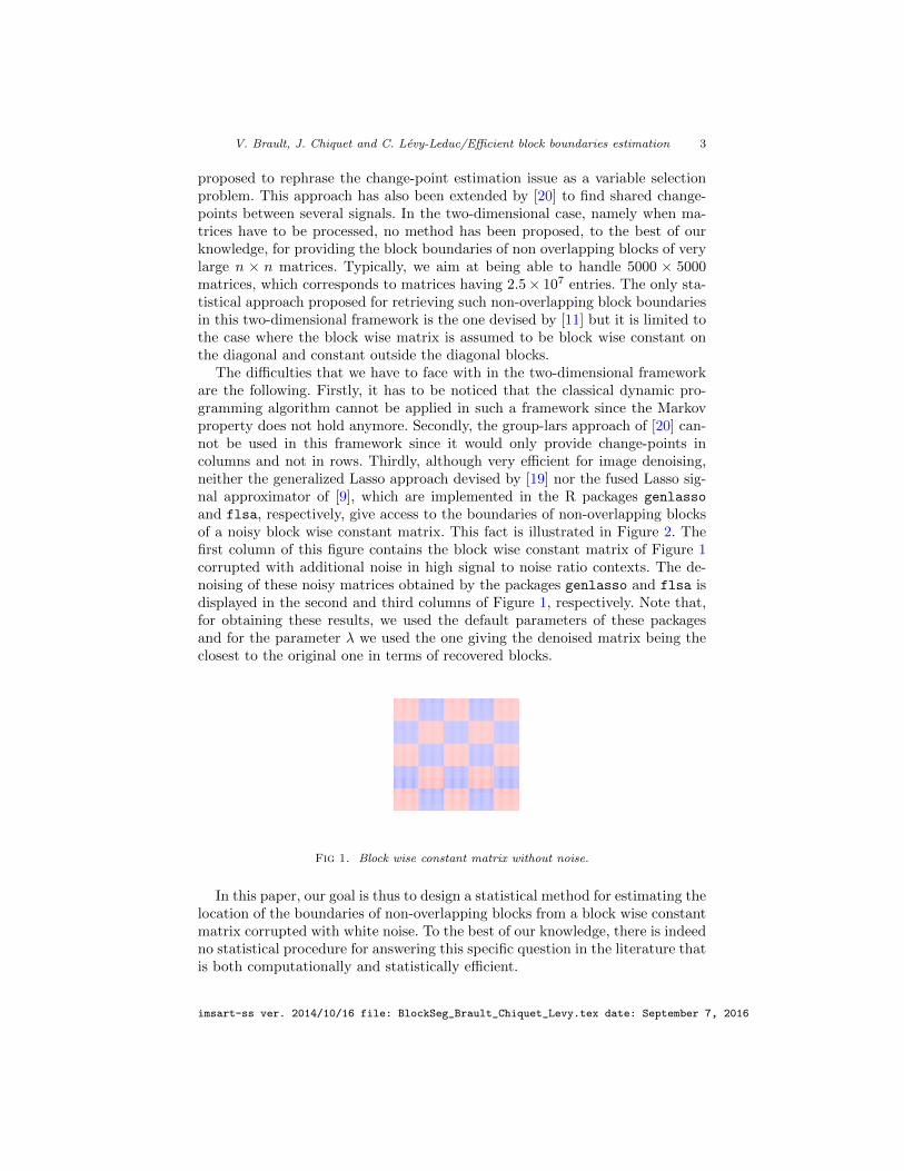
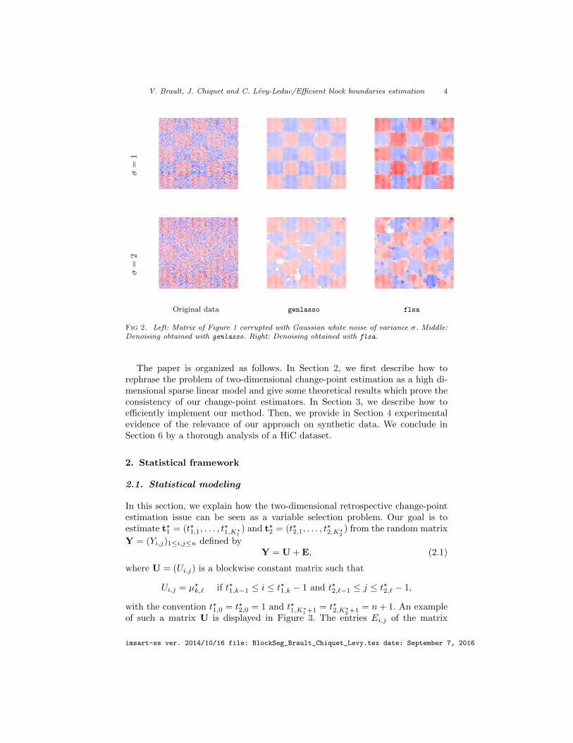
and flsa, respectively, give access to the boundaries of non-overlapping blocksof a noisy block wise constant matrix. This fact is illustrated in Figure 2. Thefirst column of this figure contains the block wise constant matrix of Figure 1corrupted with additional noise in high signal to noise ratio contexts. The de-noising of these noisy matrices obtained by the packages genlasso and flsa isdisplayed in the second and third columns of Figure 1, respectively. Note that,for obtaining these results, we used the default parameters of these packagesand for the parameter λ we used the one giving the denoised matrix being theclosest to the original one in terms of recovered blocks.
Fig 1. Block wise constant matrix without noise.
In this paper, our goal is thus to design a statistical method for estimating thelocation of the boundaries of non-overlapping blocks from a block wise constantmatrix corrupted with white noise. To the best of our knowledge, there is indeedno statistical procedure for answering this specific question in the literature thatis both computationally and statistically efficient.
imsart-ss ver. 2014/10/16 file: BlockSeg_Brault_Chiquet_Levy.tex date: September 7, 2016
V. Brault, J. Chiquet and C. Levy-Leduc/Efficient block boundaries estimation 4
σ=
1σ=
2
Original data genlasso flsa
Fig 2. Left: Matrix of Figure 1 corrupted with Gaussian white noise of variance σ. Middle:Denoising obtained with genlasso. Right: Denoising obtained with flsa.
The paper is organized as follows. In Section 2, we first describe how torephrase the problem of two-dimensional change-point estimation as a high di-mensional sparse linear model and give some theoretical results which prove theconsistency of our change-point estimators. In Section 3, we describe how toefficiently implement our method. Then, we provide in Section 4 experimentalevidence of the relevance of our approach on synthetic data. We conclude inSection 6 by a thorough analysis of a HiC dataset.
2. Statistical framework
2.1. Statistical modeling
In this section, we explain how the two-dimensional retrospective change-pointestimation issue can be seen as a variable selection problem. Our goal is toestimate t?1 = (t?1,1, . . . , t
?1,K?
1) and t?2 = (t?2,1, . . . , t
?2,K?
2) from the random matrix
Y = (Yi,j)1≤i,j≤n defined byY = U + E, (2.1)
where U = (Ui,j) is a blockwise constant matrix such that
Ui,j = µ?k,` if t?1,k−1 ≤ i ≤ t?1,k − 1 and t?2,`−1 ≤ j ≤ t?2,` − 1,
with the convention t?1,0 = t?2,0 = 1 and t?1,K?1+1 = t?2,K?
2+1 = n+ 1. An exampleof such a matrix U is displayed in Figure 3. The entries Ei,j of the matrix
imsart-ss ver. 2014/10/16 file: BlockSeg_Brault_Chiquet_Levy.tex date: September 7, 2016
V. Brault, J. Chiquet and C. Levy-Leduc/Efficient block boundaries estimation 5
E = (Ei,j)1≤i,j≤n are iid zero-mean random variables. With such a definition theYi,j are assumed to be independent random variables with a blockwise constantmean.
t?2,1
t?1,1
t?2,2
t?1,2
t?2,3
t?1,K?
1
t?2,K?
2t?2,K?
2+1
t?1,K?
1+1
t?2,0
t?1,0
µ?1,1 µ?1,2 µ?1,3 µ?1,4 µ?1,5
µ?2,1 µ?2,2 µ?2,3 µ?2,4 µ?2,5
µ?3,1 µ?3,2 µ?3,3 µ?3,4 µ?3,5
µ?4,1 µ?4,2 µ?4,3 µ?4,4 µ?4,5
t?2,1
t?1,1
t?2,2
t?1,2
t?2,3
t?1,K?
1
t?2,K?
2t?2,K?
2+1
t?1,K?
1+1
t?2,0
t?1,0B1,1 B1,5 B1,8 B1,10 B1,13
B7,1 B7,5 B7,8 B7,10 B7,13
B11,1 B11,5 B11,8B11,10 B11,13
B13,1 B13,5 B13,8B13,10 B13,13
0
0
0
0
0
0
0
0
0
0
0
0
0
0
0
0
0
0
0
0
0
0
0
0
0
0
0
0
0
0
0
0
0
0
0
0
0
0
0
0
0
0
0
0
0
0
0
0
0
0
0
0
0
0
0
0
0
0
0
0
0
0
0
0
0
0
0
0
0
0
0
0
0
0
0
0
0
0
0
0
0
0
0
0
0
0
0
0
0
0
0
0
0
0
0
0
0
0
0
0
0
0
0
0
0
0
0
0
0
0
0
0
0
0
0
0
0
0
0
0
0
0
0
0
0
0
0
0
0
0
0
0
0
0
0
0
0
0
0
0
0
0
0
0
0
0
0
0
0
0
0
0
0
0
0
0
0
0
0
0
0
0
0
0
0
0
0
0
0
0
0
0
0
0
0
0
0
0
0
0
0
0
0
0
0
0
0
0
0
0
0
0
0
0
0
0
0
0
0
0
0
0
0
0
0
0
0
0
0
0
0
0
0
0
0
0
0
0
0
0
0
0
0
0
0
0
0
0
0
0
0
0
0
0
0
0
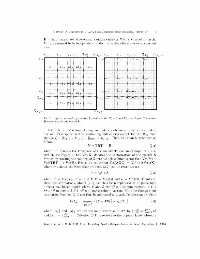
Fig 3. Left: An example of a matrix U with n = 16, K?1 = 3 and K?
2 = 4. Right: The matrixB associated to this matrix U.
Let T be a n × n lower triangular matrix with nonzero elements equal toone and B a sparse matrix containing null entries except for the Bi,j suchthat (i, j) ∈ {t?1,0, . . . , t?1,K?
1}× {t?2,0, . . . , t?2,K?
2}. Then, (2.1) can be rewritten as
follows:Y = TBT> + E, (2.2)
where T> denotes the transpose of the matrix T. For an example of a ma-trix B, see Figure 3. Let Vec(X) denotes the vectorization of the matrix Xformed by stacking the columns of X into a single column vector then Vec(Y) =Vec(TBT>) + Vec(E). Hence, by using that Vec(AXC) = (C> ⊗ A)Vec(X),where ⊗ denotes the Kronecker product, (2.2) can be rewritten as:
Y = XB + E , (2.3)
where Y = Vec(Y), X = T ⊗ T, B = Vec(B) and E = Vec(E). Thanks tothese transformations, Model (2.1) has thus been rephrased as a sparse highdimensional linear model where Y and E are n2 × 1 column vectors, X is an2 × n2 matrix and B is n2 × 1 sparse column vectors. Multiple change-pointestimation Problem (2.1) can thus be addressed as a variable selection problem:
B(λn) = ArgminB∈Rn2
{‖Y − XB‖22 + λn‖B‖1
}, (2.4)
where ‖u‖22 and ‖u‖1 are defined for a vector u in RN by ‖u‖22 =∑Ni=1 u
2i
and ‖u‖1 =∑Ni=1 |ui|. Criterion (2.4) is related to the popular Least Absolute
imsart-ss ver. 2014/10/16 file: BlockSeg_Brault_Chiquet_Levy.tex date: September 7, 2016

V. Brault, J. Chiquet and C. Levy-Leduc/Efficient block boundaries estimation 6
Shrinkage and Selection Operator (LASSO) in least-square regression. Thanks to
the sparsity enforcing property of the `1-norm, the estimator B of B is expectedto be sparse and to have non-zero elements matching with those of B. Hence,retrieving the positions of the non zero elements of B thus provides estimatorsof (t?1,k)1≤k≤K?
1and of (t?2,k)1≤k≤K?
2. More precisely, let us define by A(λn) the
set of active variables:
A(λn) ={j ∈ {1, . . . , n2} : Bj(λn) 6= 0
}.
For each j in A(λn), consider the Euclidean division of (j − 1) by n, namely(j − 1) = nqj + rj then
t1 = (t1,k)1≤k≤|A1(λn)| ∈ {rj + 1 : j ∈ A(λn)},
t2 = (t2,`)1≤`≤|A2(λn)| ∈ {qj + 1 : j ∈ A(λn)}
where t1,1 < t1,2 < · · · < t1,|A1(λn)|, t2,1 < t2,2 < · · · < t2,|A2(λn)|. (2.5)
In (2.5), |A1(λn)| and |A2(λn)| correspond to the number of distinct elements
in {rj : j ∈ A(λn)} and {qj : j ∈ A(λn)}, respectively.As far as we know, neither thorough practical implementation nor theoretical
grounding have been given so far to support such an approach for change-pointestimation in the two-dimensional case. In the following section, we give theo-retical results supporting the use of such an approach.
2.2. Theoretical results
In order to establish the consistency of the estimators t1 and t2 defined in(2.5), we shall use assumptions (A1–A4). These assumptions involve the twofollowing quantities
I?min = min0≤k≤K?
1
|t?1,k+1 − t?1,k| ∧ min0≤k≤K?
2
|t?2,k+1 − t?2,k|,
J?min = min1≤k≤K?
1 ,1≤`≤K?2+1|µ?k+1,` − µ?k,`| ∧ min
1≤k≤K?1+1,1≤`≤K?
2
|µ?k,`+1 − µ?k,`|,
which corresponds to the smallest length between two consecutive change-pointsand to the smallest jump size between two consecutive blocks, respectively.
(A1) The random variables (Ei,j)1≤i,j≤n are iid zero mean random variablessuch that there exists a positive constant β such that for all ν in R,E[exp(νE1,1)] ≤ exp(βν2).
(A2) The sequence (λn) appearing in (2.4) is such that (nδnJ?min)−1λn → 0, as
n tends to infinity.
(A3) The sequence (δn) is a non increasing and positive sequence tending tozero such that nδnJ
?min
2/ log(n)→∞, as n tends to infinity.
imsart-ss ver. 2014/10/16 file: BlockSeg_Brault_Chiquet_Levy.tex date: September 7, 2016
V. Brault, J. Chiquet and C. Levy-Leduc/Efficient block boundaries estimation 7
(A4) I?min ≥ nδn.
Proposition 1. Let (Yi,j)1≤i,j≤n be defined by (2.1) and t1,k, t2,k be defined
by (2.5). Assume that |A1(λn)| = K?1 and that |A2(λn)| = K?
2 , with probabiltytending to one, then,
P({
max1≤k≤K?
1
∣∣t1,k − t?1,k∣∣ ≤ nδn} ∩{ max1≤k≤K?
2
∣∣t2,k − t?2,k∣∣ ≤ nδn})→ 1,
as n→∞. (2.6)
The proof of Proposition 1 is based on the two following lemmas. The firstone comes from the Karush-Kuhn-Tucker conditions of the optimization prob-lem stated in (2.4). The second one allows us to control the supremum of theempirical mean of the noise.
Lemma 2. Let (Yi,j)1≤i,j≤n be defined by (2.1). Then, U = XB, where X and
B are defined in (2.3) and (2.4) respectively, is such that
n∑k=rj+1
n∑`=qj+1
Yk,` −n∑
k=rj+1
n∑`=qj+1
Uk,` =λn2
sign(Bj), if Bj 6= 0, (2.7)
∣∣∣∣∣∣n∑
k=rj+1
n∑`=qj+1
Yk,` −n∑
k=rj+1
n∑`=qj+1
Uk,`
∣∣∣∣∣∣ ≤ λn2, if Bj = 0, (2.8)
where qj and rj are the quotient and the remainder of the Euclidean division of(j − 1) by n, respectively, that is (j − 1) = nqj + rj. In (2.7), sign denotes thefunction which is defined by sign(x) = 1, if x > 0, −1, if x < 0 and 0 if x = 0.
Moreover, the matrix U, which is such that U = Vec(U), is blockwise constant
and satisfies Ui,j = µk,`, if t1,k−1 ≤ i ≤ t1,k − 1 and t2,`−1 ≤ j ≤ t2,` − 1,
k ∈ {1, . . . , |A1(λn)|}, ` ∈ {1, . . . , |A2(λn)|}, where the t1,k, t2,k, A1(λn) and
A2(λn) are defined in (2.5).
Lemma 3. Let (Ei,j)1≤i,j≤n be random variables satisfying (A1). Let also (vn)and (xn) be two positive sequences such that vnx
2n/ log(n)→∞, then
P
max1≤rn<sn≤n
|rn−sn|≥vn
∣∣∣∣∣∣(sn − rn)−1sn−1∑j=rn
En,j
∣∣∣∣∣∣ ≥ xn→ 0, as n→∞,
the result remaining valid if En,j is replaced by Ej,n.
The proofs of Proposition 1, Lemmas 2 and 3 are given in Section A.
Remark. If Y is a non square matrix having n1 rows and n2 columns, with n1 6=n2, the result of Proposition 1 remains valid if in Assumption (A3) δn is replacedby δn1,n2 satisfying n1δn1,n2J
?min
2/ log(n2) → ∞ and n2δn1,n2J?min
2/ log(n1) →∞, as n1 and n2 tend to infinity.
imsart-ss ver. 2014/10/16 file: BlockSeg_Brault_Chiquet_Levy.tex date: September 7, 2016
V. Brault, J. Chiquet and C. Levy-Leduc/Efficient block boundaries estimation 8
3. Implementation
In order to identify a series of change-points we look for the whole path ofsolutions in (2.4), i.e., {B(λ), λmin < λ < λmax} such that |A(λmax)| = 0 and|A(λmin)| = s with s a predefined maximal number of activated variables. Tothis end it is natural to adopt the famous homotopy/LARS strategy of [16, 5].Such an algorithm identifies in Problem (2.4) the successive values of λ thatcorrespond to the activation of a new variable, or the deletion of one that becameirrelevant. However, the existing implementations do not apply here since thesize of the design matrix X – even for reasonable n – is challenging both interms of memory requirement and computational burden. To overcome theselimitations, we need to take advantage of the particular structure of the problem.In the following lemmas (which are proved in Section A), we show that the mostinvolving computations in the LARS can be made extremely efficiently thanksto the particular structure of X .
Lemma 4. For any vector v ∈ Rn2
, computing Xv and X>v requires at worse2n2 operations.
Lemma 5. Let A = {a1, . . . , aK} and for each j in A let us consider theEuclidean division of j − 1 by n given by j − 1 = nqj + rj, then((X>X
)A,A
)1≤k,`≤K
= ((n− (qak ∨ qa`))× (n− (rak ∨ ra`)))1≤k,`≤K . (3.1)
Moreover, for any non empty subset A of distinct indices in{
1, . . . , n2}
, thematrix X>AXA is invertible.
Lemma 6. Assume that we have at our disposal the Cholesky factorization ofX>AXA. The updated factorization on the extended set A ∪ {j} only requiressolving a |A|-size triangular system, with complexity O(|A|2). Moreover, thedowndated factorization on the restricted set A\{j} requires a rotation withnegligible cost to preserve the triangular form of the Cholesky factorization aftera column deletion.
Remark. We were able to obtain a closed-form expression of the inverse (X>AXA)−1
for some special cases of the subset A, namely, when the quotients/ratios as-sociated with the Euclidean divisions of the elements of A are endowed witha particular ordering. Moreover, for addressing any general problem, we rathersolve systems involving X>AXA by means of a Cholesky factorization which isupdated along the homotopy algorithm. These updates correspond to adding orremoving an element at a time in A and are performed efficiently as stated inLemma 6.
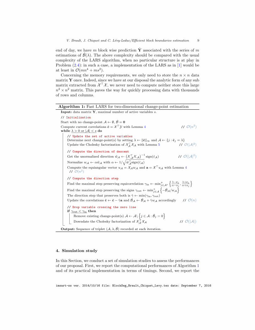
These lemmas are the building blocks for our LARS implementation givenin Algorithm 1, where we detail the leading complexity associated with eachpart. The global complexity is in O(mn2 + ms2) where m is the final numberof steps in the while loop. These steps include all the successive additions anddeletions needed to reach s, the final targeted number of active variables. At the
imsart-ss ver. 2014/10/16 file: BlockSeg_Brault_Chiquet_Levy.tex date: September 7, 2016
V. Brault, J. Chiquet and C. Levy-Leduc/Efficient block boundaries estimation 9
end of day, we have m block wise prediction Y associated with the series of mestimations of B(λ). The above complexity should be compared with the usualcomplexity of the LARS algorithm, when no particular structure is at play inProblem (2.4): in such a case, a implementation of the LARS as in [1] would beat least in O(mn4 +ms2).
Concerning the memory requirements, we only need to store the n× n datamatrix Y once. Indeed, since we have at our disposal the analytic form of any submatrix extracted from X>X , we never need to compute neither store this largen2 × n2 matrix. This paves the way for quickly processing data with thousandsof rows and columns.
Algorithm 1: Fast LARS for two-dimensional change-point estimationInput: data matrix Y, maximal number of active variables s.
// Initialization
Start with no change-point A ← ∅, B = 0
Compute current correlations c = X>Y with Lemma 4 // O(n2)while λ > 0 or |A| < s do
// Update the set of active variables
Determine next change-point(s) by setting λ← ‖c‖∞ and A ← {j : cj = λ}Update the Cholesky factorization of X>AXA with Lemma 5 // O(|A|2)
// Compute the direction of descent
Get the unormalized direction wA ←(X>·AX·A
)−1sign(cA) // O(|A|2)
Normalize wA ← αwA with α← 1/√w>Asign(cA)
Compute the equiangular vector uA = XAwA and a = X>uA with Lemma 4// O(n2)
// Compute the direction step
Find the maximal step preserving equicorrelation γin ← min+j∈Ac
{λ−cjα−aj
,λ+cjα+aj
}Find the maximal step preserving the signs γout ← min+
j∈A
{−BA/wA
}The direction step that preserves both is γ ← min(γin, γout)
Update the correlations c← c− γa and BA ← BA + γwA accordingly // O(n)
// Drop variable crossing the zero line
if γout < γin then
Remove existing change-point(s) A ← A\{j ∈ A : Bj = 0
}Downdate the Cholesky factorization of X>AXA // O(|A|)
Output: Sequence of triplet (A, λ, B) recorded at each iteration.
4. Simulation study
In this Section, we conduct a set of simulation studies to assess the performancesof our proposal. First, we report the computational performances of Algorithm 1and of its practical implementation in terms of timings. Second, we report the
imsart-ss ver. 2014/10/16 file: BlockSeg_Brault_Chiquet_Levy.tex date: September 7, 2016
V. Brault, J. Chiquet and C. Levy-Leduc/Efficient block boundaries estimation 10
statistical performances of our estimators (2.5) for recovering the true change-points by means of Receiver Operating Characteristic (ROC) curves.
4.1. Data generation
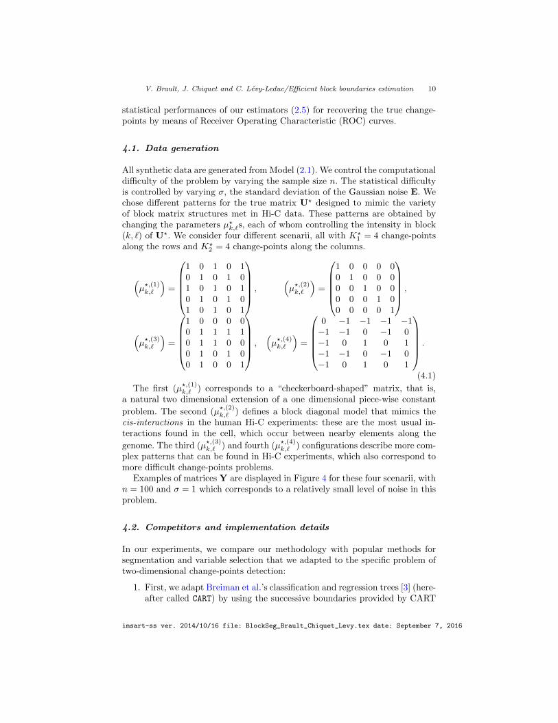
All synthetic data are generated from Model (2.1). We control the computationaldifficulty of the problem by varying the sample size n. The statistical difficultyis controlled by varying σ, the standard deviation of the Gaussian noise E. Wechose different patterns for the true matrix U? designed to mimic the varietyof block matrix structures met in Hi-C data. These patterns are obtained bychanging the parameters µ?k,`s, each of whom controlling the intensity in block(k, `) of U?. We consider four different scenarii, all with K?
1 = 4 change-pointsalong the rows and K?
2 = 4 change-points along the columns.
(µ?,(1)k,`
)=
1 0 1 0 10 1 0 1 01 0 1 0 10 1 0 1 01 0 1 0 1
,(µ?,(2)k,`
)=
1 0 0 0 00 1 0 0 00 0 1 0 00 0 0 1 00 0 0 0 1
,
(µ?,(3)k,`
)=
1 0 0 0 00 1 1 1 10 1 1 0 00 1 0 1 00 1 0 0 1
,(µ?,(4)k,`
)=
0 −1 −1 −1 −1−1 −1 0 −1 0−1 0 1 0 1−1 −1 0 −1 0−1 0 1 0 1
.
(4.1)
The first (µ?,(1)k,` ) corresponds to a “checkerboard-shaped” matrix, that is,
a natural two dimensional extension of a one dimensional piece-wise constant
problem. The second (µ?,(2)k,` ) defines a block diagonal model that mimics the
cis-interactions in the human Hi-C experiments: these are the most usual in-teractions found in the cell, which occur between nearby elements along the
genome. The third (µ?,(3)k,` ) and fourth (µ
?,(4)k,` ) configurations describe more com-
plex patterns that can be found in Hi-C experiments, which also correspond tomore difficult change-points problems.
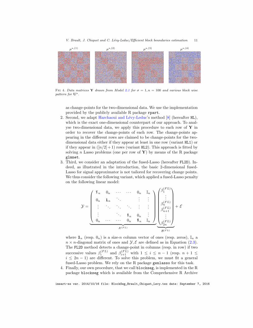
Examples of matrices Y are displayed in Figure 4 for these four scenarii, withn = 100 and σ = 1 which corresponds to a relatively small level of noise in thisproblem.
4.2. Competitors and implementation details
In our experiments, we compare our methodology with popular methods forsegmentation and variable selection that we adapted to the specific problem oftwo-dimensional change-points detection:
1. First, we adapt Breiman et al.’s classification and regression trees [3] (here-after called CART) by using the successive boundaries provided by CART
imsart-ss ver. 2014/10/16 file: BlockSeg_Brault_Chiquet_Levy.tex date: September 7, 2016
V. Brault, J. Chiquet and C. Levy-Leduc/Efficient block boundaries estimation 11
µ?,(1) µ?,(2) µ?,(3) µ?,(4)
Fig 4. Data matrices Y drawn from Model 2.1 for σ = 1, n = 100 and various block wisepattern for U?.
as change-points for the two-dimensional data. We use the implementationprovided by the publicly available R package rpart.
2. Second, we adapt Harchaoui and Levy-Leduc’s method [8] (hereafter HL),which is the exact one-dimensional counterpart of our approach. To anal-yse two-dimensional data, we apply this procedure to each row of Y inorder to recover the change-points of each row. The change-points ap-pearing in the different rows are claimed to be change-points for the two-dimensional data either if they appear at least in one row (variant HL1) orif they appear in ([n/2] + 1) rows (variant HL2). This approach is fitted bysolving n Lasso problems (one per row of Y) by means of the R packageglmnet.
3. Third, we consider an adaptation of the fused-Lasso (hereafter FL2D). In-deed, as illustrated in the introduction, the basic 2-dimensional fused-Lasso for signal approximator is not tailored for recovering change points.We thus consider the following variant, which applied a fused-Lasso penaltyon the following linear model:
Y =
1n 0n · · · · · · 0n In
0n 1n. . .
......
.... . .
. . .. . .
......
.... . . 1n 0n
...0n · · · · · · 0n 1n In
︸ ︷︷ ︸
X (FL)
β(FL)1...
β(FL)n
β(FL)n+1...
β(FL)2n
︸ ︷︷ ︸B(FL)
+ E
where 1n (resp. 0n) is a size-n column vector of ones (resp. zeros), In an × n-diagonal matrix of ones and Y, E are defined as in Equation (2.3).The FL2D method detects a change-point in columns (resp. in row) if two
successive values β(FL)i and β
(FL)i+1 with 1 ≤ i ≤ n − 1 (resp. n + 1 ≤
i ≤ 2n − 1) are different. To solve this problem, we must fit a generalfused-Lasso problem. We rely on the R package genlasso for this task.
4. Finally, our own procedure, that we call blockseg, is implemented in the Rpackage blockseg which is available from the Comprehensive R Archive
imsart-ss ver. 2014/10/16 file: BlockSeg_Brault_Chiquet_Levy.tex date: September 7, 2016
V. Brault, J. Chiquet and C. Levy-Leduc/Efficient block boundaries estimation 12
Network (CRAN, [17]). Most of the computation are performed in C++
using the library armadillo for linear algebra [18].
In what follows, all experiments were conducted on a Linux workstation withIntel Xeon 2.4 GHz processor and 8 GB of memory.
4.3. Numerical performances
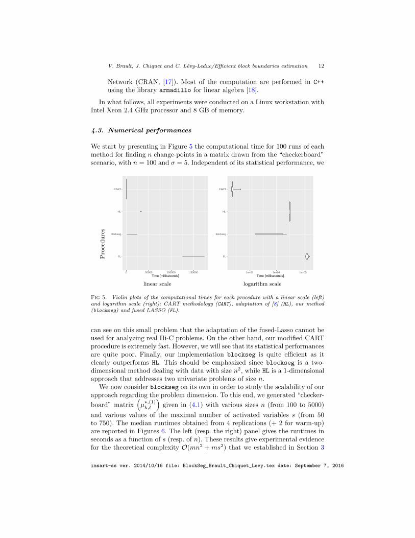
We start by presenting in Figure 5 the computational time for 100 runs of eachmethod for finding n change-points in a matrix drawn from the “checkerboard”scenario, with n = 100 and σ = 5. Independent of its statistical performance, we
Procedures
FL
blockseg
HL
CART
0 50000 100000 150000Time [milliseconds]
FL
blockseg
HL
CART
1e+03 1e+04 1e+05Time [milliseconds]
linear scale logarithm scale
Fig 5. Violin plots of the computational times for each procedure with a linear scale (left)and logarithm scale (right): CART methodology (CART), adaptation of [8] (HL), our method(blockseg) and fused LASSO (FL).
can see on this small problem that the adaptation of the fused-Lasso cannot beused for analyzing real Hi-C problems. On the other hand, our modified CARTprocedure is extremely fast. However, we will see that its statistical performancesare quite poor. Finally, our implementation blockseg is quite efficient as itclearly outperforms HL. This should be emphasized since blockseg is a two-dimensional method dealing with data with size n2, while HL is a 1-dimensionalapproach that addresses two univariate problems of size n.
We now consider blockseg on its own in order to study the scalability of ourapproach regarding the problem dimension. To this end, we generated “checker-
board” matrix(µ?,(1)k,`
)given in (4.1) with various sizes n (from 100 to 5000)
and various values of the maximal number of activated variables s (from 50to 750). The median runtimes obtained from 4 replications (+ 2 for warm-up)are reported in Figures 6. The left (resp. the right) panel gives the runtimes inseconds as a function of s (resp. of n). These results give experimental evidencefor the theoretical complexity O(mn2 + ms2) that we established in Section 3
imsart-ss ver. 2014/10/16 file: BlockSeg_Brault_Chiquet_Levy.tex date: September 7, 2016
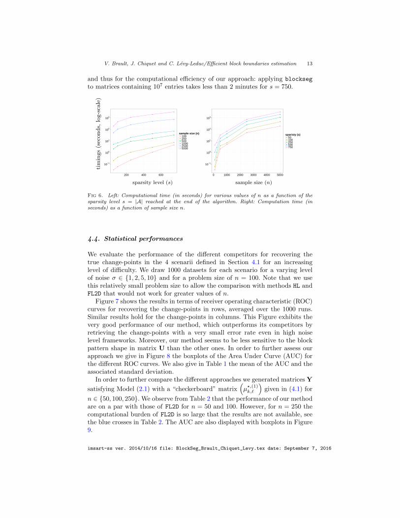
V. Brault, J. Chiquet and C. Levy-Leduc/Efficient block boundaries estimation 13
and thus for the computational efficiency of our approach: applying blockseg
to matrices containing 107 entries takes less than 2 minutes for s = 750.
timings(seconds,
log-scale)
●
●
●
●
●
●
●
●
●
●
●
●
●
●
●
●
●
●
●
●
●
●
●
●
●
●
●
●
●
●
10−1
100
101
102
103
200 400 600
sample size (n)●
●
●
●
●
●
100250500100025005000
●
●
●
●
●
●
●
●
●
●
●
●
●
●
●
●
●
●
●
●
●
●
●
●
●
●
●
●
●
●
10−1
100
101
102
103
0 1000 2000 3000 4000 5000
sparisty (s)●
●
●
●
●
50100250500750
sparsity level (s) sample size (n)
Fig 6. Left: Computational time (in seconds) for various values of n as a function of thesparsity level s = |A| reached at the end of the algorithm. Right: Computation time (inseconds) as a function of sample size n.
4.4. Statistical performances
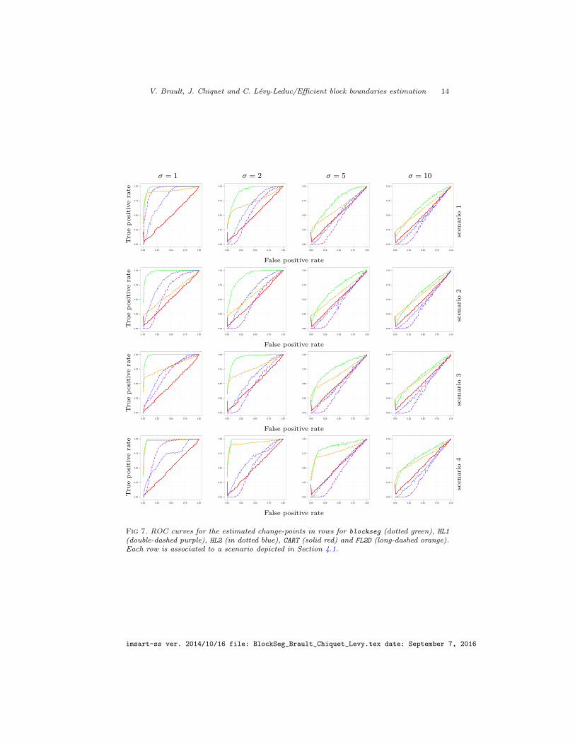
We evaluate the performance of the different competitors for recovering thetrue change-points in the 4 scenarii defined in Section 4.1 for an increasinglevel of difficulty. We draw 1000 datasets for each scenario for a varying levelof noise σ ∈ {1, 2, 5, 10} and for a problem size of n = 100. Note that we usethis relatively small problem size to allow the comparison with methods HL andFL2D that would not work for greater values of n.
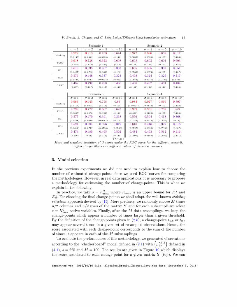
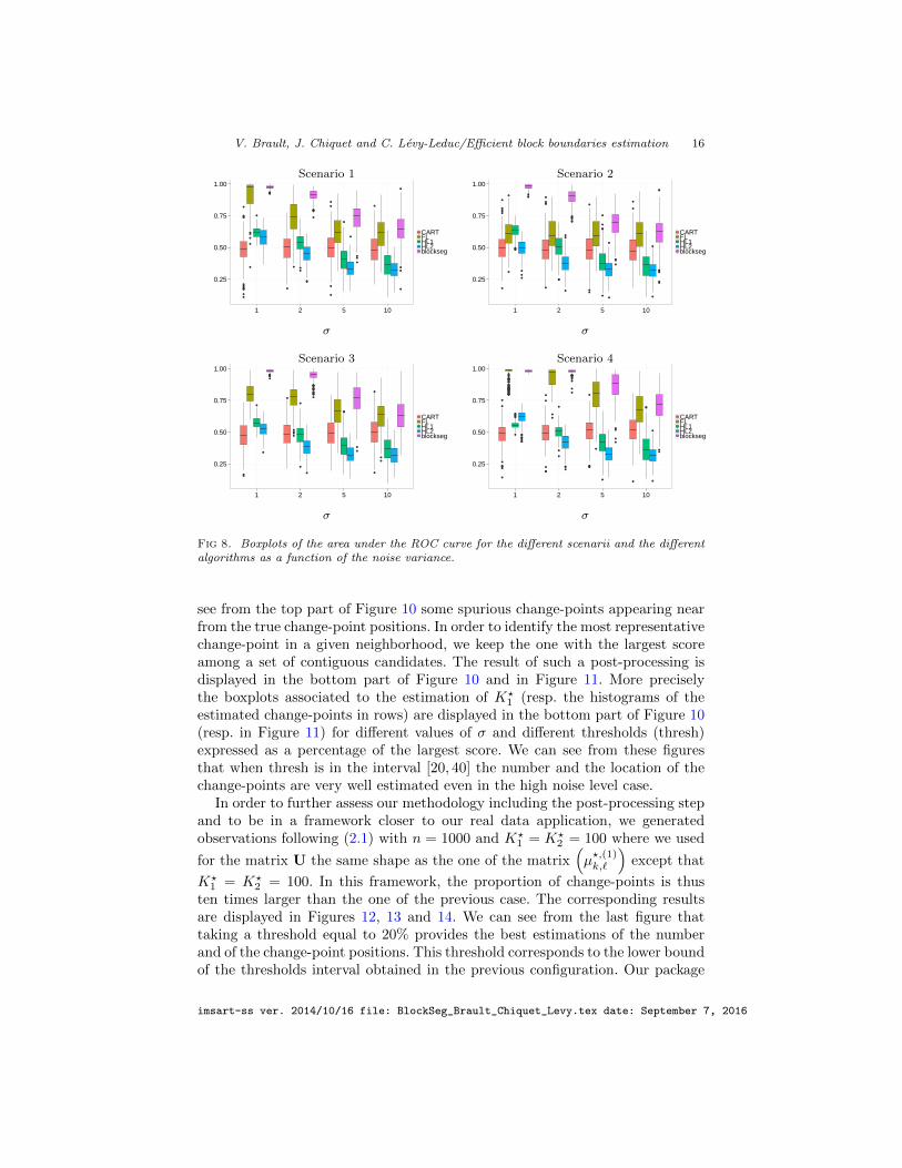
Figure 7 shows the results in terms of receiver operating characteristic (ROC)curves for recovering the change-points in rows, averaged over the 1000 runs.Similar results hold for the change-points in columns. This Figure exhibits thevery good performance of our method, which outperforms its competitors byretrieving the change-points with a very small error rate even in high noiselevel frameworks. Moreover, our method seems to be less sensitive to the blockpattern shape in matrix U than the other ones. In order to further assess ourapproach we give in Figure 8 the boxplots of the Area Under Curve (AUC) forthe different ROC curves. We also give in Table 1 the mean of the AUC and theassociated standard deviation.
In order to further compare the different approaches we generated matrices Y
satisfying Model (2.1) with a “checkerboard” matrix(µ?,(1)k,`
)given in (4.1) for
n ∈ {50, 100, 250}. We observe from Table 2 that the performance of our methodare on a par with those of FL2D for n = 50 and 100. However, for n = 250 thecomputational burden of FL2D is so large that the results are not available, seethe blue crosses in Table 2. The AUC are also displayed with boxplots in Figure9.
imsart-ss ver. 2014/10/16 file: BlockSeg_Brault_Chiquet_Levy.tex date: September 7, 2016
V. Brault, J. Chiquet and C. Levy-Leduc/Efficient block boundaries estimation 14
σ = 1 σ = 2 σ = 5 σ = 10
Tru
epositivera
te
0.00
0.25
0.50
0.75
1.00
0.00 0.25 0.50 0.75 1.00
0.00
0.25
0.50
0.75
1.00
0.00 0.25 0.50 0.75 1.00
0.00
0.25
0.50
0.75
1.00
0.00 0.25 0.50 0.75 1.00
0.00
0.25
0.50
0.75
1.00
0.00 0.25 0.50 0.75 1.00
scenario1
False positive rate
Tru
epositivera
te
0.00
0.25
0.50
0.75
1.00
0.00 0.25 0.50 0.75 1.00
0.00
0.25
0.50
0.75
1.00
0.00 0.25 0.50 0.75 1.00
0.00
0.25
0.50
0.75
1.00
0.00 0.25 0.50 0.75 1.00
0.00
0.25
0.50
0.75
1.00
0.00 0.25 0.50 0.75 1.00
scenario2
False positive rate
Tru
epositivera
te
0.00
0.25
0.50
0.75
1.00
0.00 0.25 0.50 0.75 1.00
0.00
0.25
0.50
0.75
1.00
0.00 0.25 0.50 0.75 1.00
0.00
0.25
0.50
0.75
1.00
0.00 0.25 0.50 0.75 1.00
0.00
0.25
0.50
0.75
1.00
0.00 0.25 0.50 0.75 1.00
scenario3
False positive rate
Tru
epositivera
te
0.00
0.25
0.50
0.75
1.00
0.00 0.25 0.50 0.75 1.00
0.00
0.25
0.50
0.75
1.00
0.00 0.25 0.50 0.75 1.00
0.00
0.25
0.50
0.75
1.00
0.00 0.25 0.50 0.75 1.00
0.00
0.25
0.50
0.75
1.00
0.00 0.25 0.50 0.75 1.00
scenario4
False positive rate
Fig 7. ROC curves for the estimated change-points in rows for blockseg (dotted green), HL1(double-dashed purple), HL2 (in dotted blue), CART (solid red) and FL2D (long-dashed orange).Each row is associated to a scenario depicted in Section 4.1.
imsart-ss ver. 2014/10/16 file: BlockSeg_Brault_Chiquet_Levy.tex date: September 7, 2016
V. Brault, J. Chiquet and C. Levy-Leduc/Efficient block boundaries estimation 15
Scenario 1 Scenario 2σ = 1 σ = 2 σ = 5 σ = 10 σ = 1 σ = 2 σ = 5 σ = 10
blockseg0.972 0.913 0.733 0.644 0.977 0.896 0.689 0.617
(0.0145) (0.0421) (0.0988) (0.118) (0.0206) (0.0555) (0.107) (0.123)
FL2D0.918 0.738 0.623 0.608 0.608 0.603 0.601 0.603(0.102) (0.139) (0.127) (0.13) (0.116) (0.125) (0.127) (0.127)
HL10.618 0.535 0.407 0.363 0.635 0.505 0.382 0.351
(0.0427) (0.0708) (0.102) (0.108) (0.0535) (0.0874) (0.105) (0.107)
HL20.576 0.448 0.337 0.323 0.498 0.374 0.326 0.317
(0.0744) (0.0713) (0.0734) (0.072) (0.0653) (0.0777) (0.0727) (0.0745)
CART0.482 0.497 0.498 0.486 0.496 0.487 0.491 0.484(0.107) (0.107) (0.117) (0.119) (0.112) (0.124) (0.126) (0.118)
Scenario 3 Scenario 4σ = 1 σ = 2 σ = 5 σ = 10 σ = 1 σ = 2 σ = 5 σ = 10
blockseg0.983 0.945 0.758 0.63 0.983 0.977 0.866 0.707
(0.0114) (0.0391) (0.113) (0.125) (0.00927) (0.0179) (0.102) (0.124)
FL2D0.799 0.772 0.667 0.623 0.969 0.931 0.789 0.68
(0.0855) (0.0956) (0.121) (0.121) (0.051) (0.0722) (0.135) (0.134)
HL10.575 0.479 0.391 0.368 0.556 0.504 0.418 0.368
(0.0458) (0.0819) (0.0981) (0.105) (0.0252) (0.0514) (0.0974) (0.11)
HL20.524 0.384 0.326 0.319 0.616 0.416 0.327 0.316
(0.0612) (0.0711) (0.0716) (0.0738) (0.0527) (0.0696) (0.0714) (0.067)
CART0.474 0.485 0.495 0.502 0.484 0.493 0.512 0.516(0.106) (0.11) (0.114) (0.115) (0.0905) (0.0889) (0.0985) (0.111)
Table 1Mean and standard deviation of the area under the ROC curve for the different scenarii,
different algorithms and different values of the noise variance.
5. Model selection
In the previous experiments we did not need to explain how to choose thenumber of estimated change-points since we used ROC curves for comparingthe methodologies. However, in real data applications, it is necessary to proposea methodology for estimating the number of change-points. This is what weexplain in the following.
In practice, we take s = K2max where Kmax is an upper bound for K?
1 andK?
2 . For choosing the final change-points we shall adapt the well-known stabilityselection approach devised by [15]. More precisely, we randomly choose M timesn/2 columns and n/2 rows of the matrix Y and for each subsample we selects = K2
max active variables. Finally, after the M data resamplings, we keep thechange-points which appear a number of times larger than a given threshold.By the definition of the change-points given in (2.5), a change-point t1,k or t2,`may appear several times in a given set of resampled observations. Hence, thescore associated with each change-point corresponds to the sum of the numberof times it appears in each of the M subsamplings.
To evaluate the performances of this methodology, we generated observations
according to the “checkerboard” model defined in (2.1) with(µ?,(1)k,`
)defined in
(4.1), s = 225 and M = 100. The results are given in Figure 10 which displaysthe score associated to each change-point for a given matrix Y (top). We can
imsart-ss ver. 2014/10/16 file: BlockSeg_Brault_Chiquet_Levy.tex date: September 7, 2016
V. Brault, J. Chiquet and C. Levy-Leduc/Efficient block boundaries estimation 16
Scenario 1 Scenario 2
●
●
●
●
●
●
●
●
●●●
●
●
●
●
●
● ●
●
●
●
●
●
●
●
●
●
●
●●
●
●●●●
●●●●
●
●
●
●
●
●
●
●
0.25
0.50
0.75
1.00
1 2 5 10
CARTFLHL1HL2blockseg
●
●
●
●
●
●
●
●
●
●
●
●
●
●
●
●
●
●
●●●●
●●
●
●
●
●
●
●
●
●
●
●
●
●
●●
●
●
●
●
●
●
●●
●
●
●
●●
●
●●
●
●
●●0.25
0.50
0.75
1.00
1 2 5 10
CARTFLHL1HL2blockseg
σ σ
Scenario 3 Scenario 4
●●
●
●
●
●
●
●
●
●
●
●
●
●
●●
●
●
●●
●
●
●●
●
●
●
●
●
●
●
●
●
●●
●
●
●
●
●
●
●
●
0.25
0.50
0.75
1.00
1 2 5 10
CARTFLHL1HL2blockseg
●
●
●
●
●
●
●●
●
●
●●
●
●●●
●
●
●
●
●
●
●●
●
●
●
●
●●
●
●
●
●
●●
●
●
●
●
●
●
●
●
●●
●
●
●
●
●
●
●
●●
●
●
●
●
●
●
●
●
●
●●
●
●
●
●
●
●●●●●
●
●
●
●
●
●●
●
●
●
●
●●
●
●
●
●●
●
●
●
●●
●
●
●
●
●●●●●
●
●
●
●
●
●
0.25
0.50
0.75
1.00
1 2 5 10
CARTFLHL1HL2blockseg
σ σ
Fig 8. Boxplots of the area under the ROC curve for the different scenarii and the differentalgorithms as a function of the noise variance.
see from the top part of Figure 10 some spurious change-points appearing nearfrom the true change-point positions. In order to identify the most representativechange-point in a given neighborhood, we keep the one with the largest scoreamong a set of contiguous candidates. The result of such a post-processing isdisplayed in the bottom part of Figure 10 and in Figure 11. More preciselythe boxplots associated to the estimation of K?
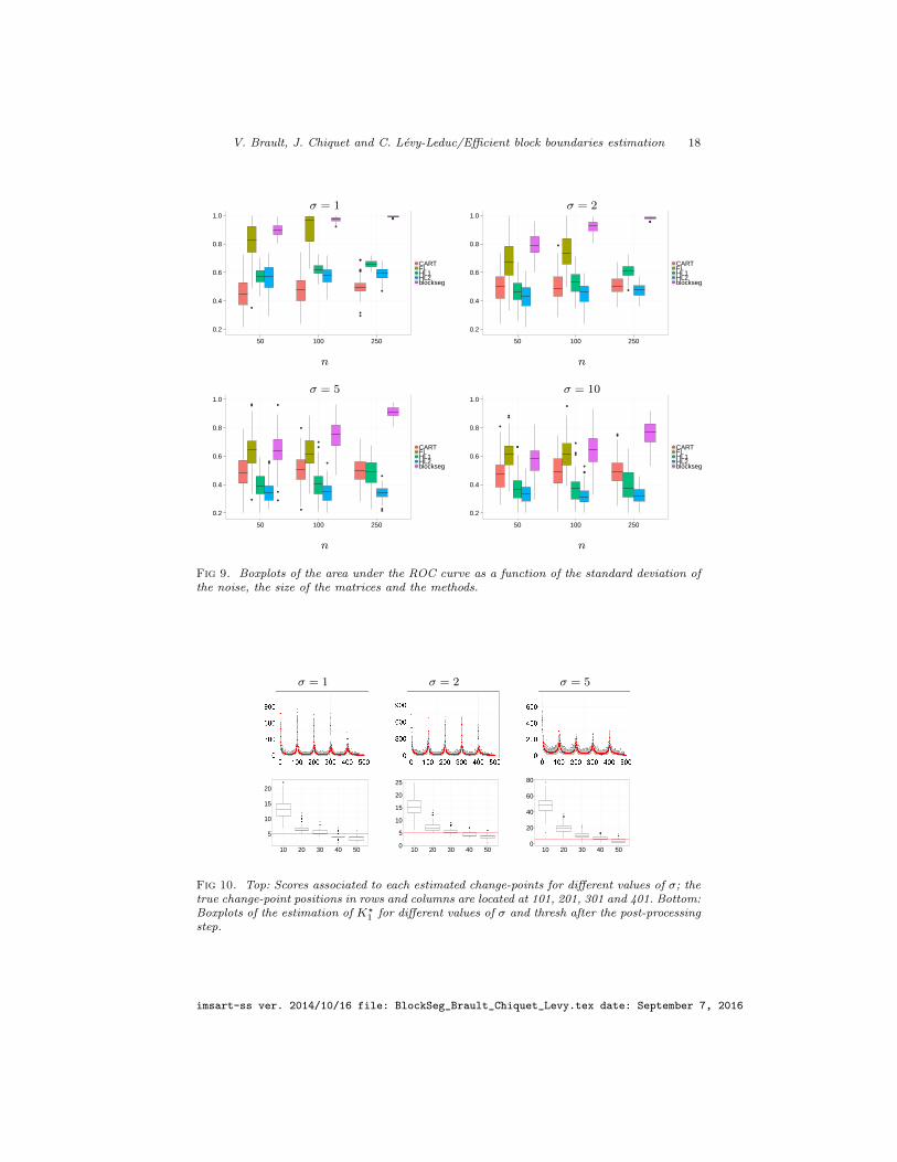
1 (resp. the histograms of theestimated change-points in rows) are displayed in the bottom part of Figure 10(resp. in Figure 11) for different values of σ and different thresholds (thresh)expressed as a percentage of the largest score. We can see from these figuresthat when thresh is in the interval [20, 40] the number and the location of thechange-points are very well estimated even in the high noise level case.
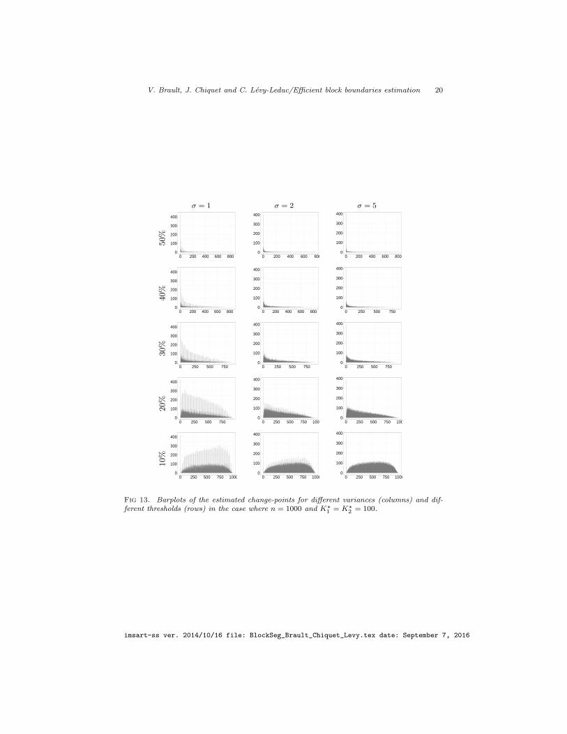
In order to further assess our methodology including the post-processing stepand to be in a framework closer to our real data application, we generatedobservations following (2.1) with n = 1000 and K?
1 = K?2 = 100 where we used
for the matrix U the same shape as the one of the matrix(µ?,(1)k,`
)except that
K?1 = K?
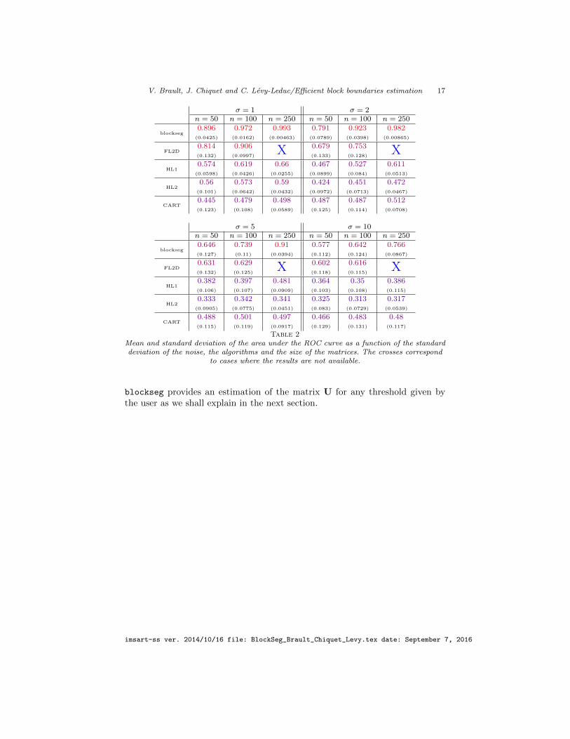
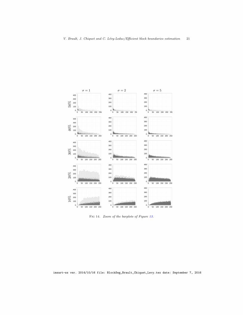
2 = 100. In this framework, the proportion of change-points is thusten times larger than the one of the previous case. The corresponding resultsare displayed in Figures 12, 13 and 14. We can see from the last figure thattaking a threshold equal to 20% provides the best estimations of the numberand of the change-point positions. This threshold corresponds to the lower boundof the thresholds interval obtained in the previous configuration. Our package
imsart-ss ver. 2014/10/16 file: BlockSeg_Brault_Chiquet_Levy.tex date: September 7, 2016
V. Brault, J. Chiquet and C. Levy-Leduc/Efficient block boundaries estimation 17
σ = 1 σ = 2n = 50 n = 100 n = 250 n = 50 n = 100 n = 250
blockseg0.896 0.972 0.993 0.791 0.923 0.982
(0.0425) (0.0162) (0.00463) (0.0789) (0.0398) (0.00865)
FL2D0.814 0.906 X 0.679 0.753 X(0.132) (0.0997) (0.133) (0.128)
HL10.574 0.619 0.66 0.467 0.527 0.611
(0.0598) (0.0426) (0.0255) (0.0899) (0.084) (0.0513)
HL20.56 0.573 0.59 0.424 0.451 0.472
(0.101) (0.0642) (0.0432) (0.0972) (0.0713) (0.0467)
CART0.445 0.479 0.498 0.487 0.487 0.512(0.123) (0.108) (0.0589) (0.125) (0.114) (0.0708)
σ = 5 σ = 10n = 50 n = 100 n = 250 n = 50 n = 100 n = 250
blockseg0.646 0.739 0.91 0.577 0.642 0.766(0.127) (0.11) (0.0394) (0.112) (0.124) (0.0867)
FL2D0.631 0.629 X 0.602 0.616 X(0.132) (0.125) (0.118) (0.115)
HL10.382 0.397 0.481 0.364 0.35 0.386(0.106) (0.107) (0.0909) (0.103) (0.108) (0.115)
HL20.333 0.342 0.341 0.325 0.313 0.317
(0.0905) (0.0775) (0.0451) (0.083) (0.0729) (0.0539)
CART0.488 0.501 0.497 0.466 0.483 0.48(0.115) (0.119) (0.0917) (0.129) (0.131) (0.117)
Table 2Mean and standard deviation of the area under the ROC curve as a function of the standarddeviation of the noise, the algorithms and the size of the matrices. The crosses correspond
to cases where the results are not available.
blockseg provides an estimation of the matrix U for any threshold given bythe user as we shall explain in the next section.
imsart-ss ver. 2014/10/16 file: BlockSeg_Brault_Chiquet_Levy.tex date: September 7, 2016
V. Brault, J. Chiquet and C. Levy-Leduc/Efficient block boundaries estimation 18
σ = 1 σ = 2
●
●
●
●
●
●
●
●
●
●
●●●
0.2
0.4
0.6
0.8
1.0
50 100 250
CARTFLHL1HL2blockseg
●
●
●●
0.2
0.4
0.6
0.8
1.0
50 100 250
CARTFLHL1HL2blockseg
n n
σ = 5 σ = 10
●
●
●●
●
●
●
●
●●
●
●
●
●
●
●
0.2
0.4
0.6
0.8
1.0
50 100 250
CARTFLHL1HL2blockseg
●
●●
●
●
●
●●
●
●
●
●
●
●
0.2
0.4
0.6
0.8
1.0
50 100 250
CARTFLHL1HL2blockseg
n n
Fig 9. Boxplots of the area under the ROC curve as a function of the standard deviation ofthe noise, the size of the matrices and the methods.
σ = 1 σ = 2 σ = 5
●●●
●
●
●
●
●●●●
●●
●●●
●
●●●●●●
●
●
●
●●●●●●
●
●●●●●●
●
●●●
●
●●
●
●●●
●●
●
●
●●
●●●
●
●
●
●●●●●
●
●●●●
●
●●●●●●●●●●
●
●●●●●
●
●
●
●
●
●●●
●
●●●●●●
●
●●●●●●
●
●●
●●
●●
●
●●
●
●●●
●
●
●
●●●●
●
●●●
●
●●●
●
●●●●●●
●
●
●
●●●●●●●●
●●●
●●●
●
●
●
●
●●●●●
●
●
●●
●
●●●
●
●●●●●●
●●
●
5
10
15
20
10 20 30 40 50
●
●●
●
●●●●●
●
●
●●
●●
●
●
●
●
●●●●●●●
●
●●●●
●
●●●
●●●●●
●●●●
●
0
5
10
15
20
25
10 20 30 40 50
●
●
●
●●●●●●
●
●
●●●●●●●●
●●
●
●
0
20
40
60
80
10 20 30 40 50
Fig 10. Top: Scores associated to each estimated change-points for different values of σ; thetrue change-point positions in rows and columns are located at 101, 201, 301 and 401. Bottom:Boxplots of the estimation of K?
1 for different values of σ and thresh after the post-processingstep.
imsart-ss ver. 2014/10/16 file: BlockSeg_Brault_Chiquet_Levy.tex date: September 7, 2016

V. Brault, J. Chiquet and C. Levy-Leduc/Efficient block boundaries estimation 19
σ = 1 σ = 2 σ = 5
50%
0
100
200
300
400
500
0 100 200 300 4000
100
200
300
400
500
0 100 200 300 4000
100
200
300
400
0 100 200 300 400
40%
0
100
200
300
400
500
0 100 200 300 4000
100
200
300
400
500
0 100 200 300 4000
100
200
300
400
0 100 200 300 400
30%
0
100
200
300
400
500
0 100 200 300 4000
100
200
300
400
500
0 100 200 300 4000
100
200
300
400
0 100 200 300 400
20%
0
100
200
300
400
500
0 100 200 300 4000
100
200
300
400
500
0 100 200 300 4000
100
200
300
400
0 100 200 300 400
10%
0
100
200
300
400
500
0 100 200 300 4000
100
200
300
400
500
0 100 200 300 4000
100
200
300
400
0 100 200 300 400
Fig 11. Barplots of the estimated change-points for different variances (columns) and dif-ferent thresholds (rows) for the model µ?,(1).
σ = 1 σ = 2 σ = 5
●
●●
●
●
●
●
●
●
●
●
●●●
●
●
●
●
●●
●
●
●
●
●●●●●
●
●
●
●
●
●
●
●●
●●●
●●●
●●●
●
●
●
●
●
●
●
●
●
●
●
●
●
●
●●●●●
●
●
●●
●
●
●●●●●
●●
●
●
0
50
100
150
10 20 30 40 50
●
●●
●
●●●
●
●
●
●
●
●
●
●
●
●
●
●
●
●
●
●●●
●
●●
●
●
●
●
●●
●
●●●●
●
●
●
●●●●●●
●
●●●
●
●●
●
●
●
●●●
●
●
●
●
●●
●
●●
●
●●●●
●
●
0
50
100
150
200
10 20 30 40 50
●
●●
●●
●
●●●
●
●●
●●
●
●●●●
●
●
●
●
●●
●
●
●
●
●
●
●
●
●
●
●
●
●●
●●●
●
●
●
●
●
●●
●●
●
●
●●
●
●
●●●●●●●●
●●
●●
●
●●●●
●
●●
●●
●
●●●
●
●
●
●●
●
●●●●
●
●
●●
0
50
100
150
200
10 20 30 40 50
Fig 12. Boxplots of the estimation of K?1 for different values of σ and thresholds (thresh)
after the post-processing step.
imsart-ss ver. 2014/10/16 file: BlockSeg_Brault_Chiquet_Levy.tex date: September 7, 2016
V. Brault, J. Chiquet and C. Levy-Leduc/Efficient block boundaries estimation 20
σ = 1 σ = 2 σ = 5
50%
0
100
200
300
400
0 200 400 600 8000
100
200
300
400
0 200 400 600 8000
100
200
300
400
0 200 400 600 800
40%
0
100
200
300
400
0 200 400 600 8000
100
200
300
400
0 200 400 600 8000
100
200
300
400
0 250 500 750
30%
0
100
200
300
400
0 250 500 7500
100
200
300
400
0 250 500 7500
100
200
300
400
0 250 500 750
20%
0
100
200
300
400
0 250 500 7500
100
200
300
400
0 250 500 750 10000
100
200
300
400
0 250 500 750 1000
10%
0
100
200
300
400
0 250 500 750 10000
100
200
300
400
0 250 500 750 10000
100
200
300
400
0 250 500 750 1000
Fig 13. Barplots of the estimated change-points for different variances (columns) and dif-ferent thresholds (rows) in the case where n = 1000 and K?
1 = K?2 = 100.
imsart-ss ver. 2014/10/16 file: BlockSeg_Brault_Chiquet_Levy.tex date: September 7, 2016
V. Brault, J. Chiquet and C. Levy-Leduc/Efficient block boundaries estimation 21
σ = 1 σ = 2 σ = 5
50%
0
100
200
300
400
0 50 100 150 200 2500
100
200
300
400
0 50 100 150 200 2500
100
200
300
400
0 50 100 150 200 250
40%
0
100
200
300
400
0 50 100 150 200 2500
100
200
300
400
0 50 100 150 200 2500
100
200
300
400
0 50 100 150 200 250
30%
0
100
200
300
400
0 50 100 150 200 2500
100
200
300
400
0 50 100 150 200 2500
100
200
300
400
0 50 100 150 200 250
20%
0
100
200
300
400
0 50 100 150 200 2500
100
200
300
400
0 50 100 150 200 2500
100
200
300
400
0 50 100 150 200 250
10%
0
100
200
300
400
0 50 100 150 200 2500
100
200
300
400
0 50 100 150 200 2500
100
200
300
400
0 50 100 150 200 250
Fig 14. Zoom of the barplots of Figure 13.
imsart-ss ver. 2014/10/16 file: BlockSeg_Brault_Chiquet_Levy.tex date: September 7, 2016
V. Brault, J. Chiquet and C. Levy-Leduc/Efficient block boundaries estimation 22
6. Application to HiC data
In this section, we apply our methodology to publicly available HiC data (http://chromosome.sdsc.edu/mouse/hi-c/download.html) already studied by [4].This technology is based on a deep sequencing approach and provides readpairs corresponding to pairs of genomic loci that physically interacts in thenucleus, see [12] for more details. The raw measurements provided by HiC datais therefore a list of pairs of locations along the chromosome, at the nucleotideresolution. These measurement are often summarized as a square matrix whereeach entry at row i and column j stands for the total number of read pairsmatching in position i and position j, respectively. Positions refer here to asequence of non-overlapping windows of equal sizes covering the genome. Thenumber of windows may vary from one study to another: [12] considered a Mbresolution, whereas [4] went deeper and used windows of 40kb (called hereafterthe resolution).
In our study, we processed the interaction matrices of Chromosomes 1 and19 of the mouse cortex at a resolution 40 kb and we compared the numberand the location of the estimated change-points found by our approach withthose obtained by [4] on the same data since no ground truth is available. Moreprecisely, in the case of Chromosome 1, n = 4930 and in the case of Chromosome19, n = 1534.
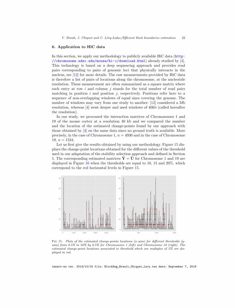
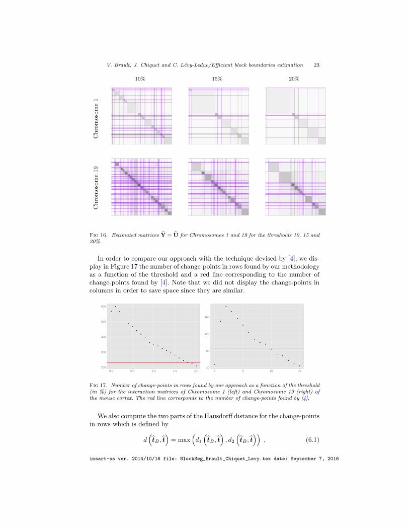
Let us first give the results obtained by using our methodology. Figure 15 dis-plays the change-point locations obtained for the different values of the thresholdused in our adaptation of the stability selection approach and defined in Section5. The corresponding estimated matrices Y = U for Chromosome 1 and 19 aredisplayed in Figure 16 when the thresholds are equal to 10, 15 and 20%, whichcorrespond to the red horizontal levels in Figure 15.
●●●●●●●●●●●●●●●●●●●●●●●●●●●●●●●●●●●●●●●● ●●●●●●●●●●●●●●●●●●●●●●●●●●●●●●● ●●●●●●●●●●●●●●●●●●●●●●●●●●●●●●●●●●●●●●●●●●●●●●●●●●●●●●●●●●●●●●●●●●●●●●●●●●●●●●●●●●●●●●●●●●●●●●●●●●●●●●●●●●●●●●●●●●●●●●●●●●●●●●●●●●●●●●●●●●●●●●●●●●●●●●●●●●●●●●●●●●●●●●●● ●●●●● ●●●●●●●●● ●●●●●●●●●●●●●●●●●●●●●●●●●●●●●●●●●●●●●●●●●●●●●●●●●●●●●●●●●●●●●● ●●●●●●●●●●●●●●●●●●● ●● ●●●●●●●●●●●●●●●●●●●●●●●●●●●●●●●●●●●●●●●●●●●●●●●● ●●●●●●●● ●● ●●●●●●●●●●●●●●●●●●●●●●●●●●●●●●●●●●●●●●●●●●●●●●● ●●●●●●●●● ●●● ●●●● ●●●●●● ●●●●●●●●●●●●●●●●●●●●●●●●●●●●●●●●●●●● ●●●● ●●●●●●●●●●●●●●●●●●●●●●●●●● ● ●●●●●●●● ●●●●●●●●● ●●●●●●●●●●●●●●●●●●●●●●●●●●●●●●●●●●●●●●●●●●●●●●●●●●●●●●●●●●●●●●●●●●●●●●●●●●● ●●●●●●●●●●●●● ●● ●●●●●●●●●●●●●●●● ●●●●●●●●●●● ●●● ●●●●● ●●●●●●●●●●●●●●●●●●●●●●●●●●●● ●●●●●●●●●●●●●●●●●●●● ●●●●●●●●●● ● ●●●●● ●●●●●●●●●●●●●●●●●●●●●●●●●●●● ●●●●●● ●● ●●●●● ●●●●●●●●●●●●●●●●●●●●●●●●● ●●●●●●● ●● ●●● ●● ●●●●●●●●●●●●●●●●●●●●●●●●●● ●● ●●●●● ●●●●●●●●●●●●●●●●●●●● ●●●●●● ●●●●●●● ●●●●●●●●●●●●●●●●●●●●●●●●●●●●●●●●●●●●●●●●●●●●●●●●●●●●●●●●●●●● ●●●●●●●●● ●●●●●●●●●●●●● ●●●●●●●● ●●● ●●● ●●●●●● ●●●●●●●●●●●●● ●●●●●●●●●●●●●●●●●●● ●●●● ●● ● ●●●●●● ●●● ●●●●●●●●●●●●●●● ●●●●●●● ●● ●●●●● ●●●● ●●●●●●●●●●●●●●●●●●●● ● ●●●●●●● ● ●●●●●●●●●●●●●●●● ●●●● ● ●●●● ●●●●●●●●●●●● ●●●●● ● ●●●● ●●●●●●●●●●●●●●●●●●●●● ●●●●●●●●●●●●●●●●● ●●●●●●● ●●●●●●● ●●●●●●●●●●●● ●●● ●●● ● ● ●●● ●●●●●●●●● ● ●●●●●●●●●●● ● ●●● ●● ● ●●●●●● ●●● ●●●●●●●●●●●●●● ●●●●●● ● ●● ●●● ●●●●●●●●●●●●●● ● ● ●●●●●●● ● ●●●●●●●●●●●●● ●●●● ● ●●●● ●●●●●●●●●●●● ●●● ●●●● ●●●●●●●●●●●●●●●●●●●●●●●●●●●● ●●●●●● ●●●●●●●●● ●●●●●●●●●● ●●● ●●● ● ● ●●● ●●●●●●●●●●● ●●●●●●● ● ●●● ● ●●●●● ● ●●●●●●●●●●●●● ●●●●●● ● ●● ●●●●●●●●●●●● ● ● ●●●●● ●●●●●●●● ● ●● ● ●●● ●●●● ●●●●●● ●●● ●●●● ●●●●●●●●●● ●●●●●●● ●● ●●●●●● ●●●●●●●● ● ●●●●●● ●●● ● ● ● ●●● ●●●●●●●● ●●●●●● ●●● ● ●●●● ● ●●●●●●●●●●● ●●●●● ● ●● ●●●●●●●●●●●● ● ● ●●●●●●●●● ● ● ●●● ●●● ●●●●● ●●● ●●●● ●●● ●●●● ●●●●● ● ●●●● ●●●●●●● ● ●●●● ●●● ● ● ● ●●● ●●●●●● ●●●●●● ● ● ●●●●● ● ●●●●●●●●●●● ●●●●● ●● ● ●●●●● ●●●●●● ● ● ●●●●●●●●● ● ● ●●● ● ●●●●● ●●● ●●●● ●● ●● ●●● ● ●●● ●●●●●●● ● ●●●● ●● ● ● ● ●●● ●●●●● ●●●●● ● ● ●●●●● ●●●●●●●●●● ●●●● ●● ● ●●●●● ●●●●●● ● ● ●●●●●●●●● ● ● ●●● ●● ● ●● ●●●● ● ●● ●● ● ●●● ● ● ●● ● ●●●● ●● ● ● ●● ●●● ●●● ● ●●●●● ●●●●●●●●●● ●●●● ● ● ●●●● ●●●●●● ● ● ●●●●●●●●● ● ● ●● ● ● ●● ●●● ● ● ●● ● ●●● ● ●● ● ●●● ●● ● ● ●● ●●● ●●● ● ●●●● ●●●●●●●●● ●●●● ● ● ●●●● ●●●●●● ● ● ●●●●●●●● ● ● ● ● ● ●●● ● ● ●●● ● ●●● ● ● ● ● ●● ● ● ●● ●●● ●●● ●●●● ●●●●●●●●● ●●●● ● ● ●●● ●●●●●● ● ● ●●●●●●●●●● ● ● ● ● ● ●●● ● ●●● ● ●●● ● ● ● ●● ● ● ●● ●●● ●●● ●●● ●●●●●●●● ●● ● ● ●●● ●●●●●●● ● ● ●●●●●●●●● ● ● ● ● ●●● ● ●●● ● ●●● ● ● ● ●● ● ● ●● ●●● ●● ●● ●●●●●●● ● ● ● ●● ●●●●●●● ● ●●●●●●●● ● ● ● ● ●● ● ●● ● ●●● ● ● ● ●● ● ● ●● ●●● ●● ●● ●●●●●●● ● ● ● ●● ●●●●●● ● ●●●●●●● ● ● ● ●● ● ● ● ●● ● ●● ● ●●● ●●● ●● ●● ●●●●●●● ● ● ● ● ●●●●●● ● ●●●●●●● ● ● ●● ● ● ● ●● ● ●●● ●● ●● ●● ●●●●●● ● ● ● ● ●●●●●● ● ●●●●●●● ● ● ●● ● ● ● ● ● ●●● ● ●● ●● ●●●●●● ● ● ● ● ●●●●●● ● ●●●●●●● ● ● ● ● ● ● ● ● ●●● ● ●● ●● ●●●●●● ● ● ● ● ●●●●●● ● ●●●●●●● ● ● ● ● ● ● ● ●● ● ●● ● ●●●●● ● ● ● ● ●●●●● ● ●●●●●●● ● ● ● ● ● ● ●● ● ●● ● ●●●●● ● ● ● ●●●●● ● ●●●●● ● ● ● ● ● ● ●● ● ● ● ●●●●● ● ● ● ●●●●● ● ●●●●● ● ● ● ● ● ●● ● ● ● ●●●●● ● ● ● ●●●●● ● ●●●●● ● ● ● ●● ● ● ● ●●●●● ● ● ● ●●●● ● ●●●●● ● ● ● ●● ● ●● ● ●●● ● ● ● ●●●● ● ●●●●● ● ● ● ●● ● ●● ● ●●● ● ● ●●● ● ●●●●● ● ● ● ●● ● ●● ● ●● ● ● ●●● ● ●●●●● ● ● ● ●● ● ●● ● ● ● ● ●●● ● ●●●●● ● ● ● ●● ● ●● ● ● ● ● ●● ● ●●●● ● ● ● ●● ● ●● ● ● ● ● ● ●●●● ● ● ● ●● ● ●● ● ● ● ●●●● ● ● ● ●● ● ●● ● ● ● ●● ● ● ●● ● ●● ● ● ● ●● ● ● ●● ●● ● ● ●● ● ● ●● ●● ● ●● ● ● ●● ●● ● ●● ● ● ●● ●● ● ●● ● ●● ●● ● ●● ● ●● ●● ● ●● ● ●● ●● ● ●● ● ●● ●● ● ●● ● ●● ●● ● ●● ● ●● ● ● ●● ● ●● ● ● ●● ● ●● ● ●● ● ●● ● ●● ● ●● ● ●● ● ●● ● ●● ● ● ● ●● ● ● ● ●● ● ● ● ●● ● ● ● ●● ● ● ● ●● ● ● ● ●● ● ● ● ●● ● ● ● ●● ● ● ●● ●● ●● ●● ●● ●● ●● ●● ●● ●● ●●●●●●●●●●●●●●●●●●●●●●●●●●●●●●●●●●●
●●●●●●●●●●●●●●●●●●●●●●●●●●●●●●●●●●●●●●●● ●●●●●●●●●●●●●●●●●●●●●●●●●●●●●●● ●●●●●●●●●●●●●●●●●●●●●●●●●●●●●●●●●●●●●●●●●●●●●●●●●●●●●●●●●●●●●●●●●●●●●●●●●●●●●●●●●●●●●●●●●●●●●●●●●●●●●●●●●●●●●●●●●●●●●●●●●●●●●●●●●●●●●●●●●●●●●●●●●●●●●●●●●●●●●●●●●●●●●●●● ●●●●● ●●●●●●●●● ●●●●●●●●●●●●●●●●●●●●●●●●●●●●●●●●●●●●●●●●●●●●●●●●●●●●●●●●●●●●●● ●●●●●●●●●●●●●●●●●●● ●● ●●●●●●●●●●●●●●●●●●●●●●●●●●●●●●●●●●●●●●●●●●●●●●●● ●●●●●●●● ●● ●●●●●●●●●●●●●●●●●●●●●●●●●●●●●●●●●●●●●●●●●●●●●●● ●●●●●●●●● ●●● ●●●● ●●●●●● ●●●●●●●●●●●●●●●●●●●●●●●●●●●●●●●●●●●● ●●●● ●●●●●●●●●●●●●●●●●●●●●●●●●● ● ●●●●●●●● ●●●●●●●●● ●●●●●●●●●●●●●●●●●●●●●●●●●●●●●●●●●●●●●●●●●●●●●●●●●●●●●●●●●●●●●●●●●●●●●●●●●●● ●●●●●●●●●●●●● ●● ●●●●●●●●●●●●●●●● ●●●●●●●●●●● ●●● ●●●●● ●●●●●●●●●●●●●●●●●●●●●●●●●●●● ●●●●●●●●●●●●●●●●●●●● ●●●●●●●●●● ● ●●●●● ●●●●●●●●●●●●●●●●●●●●●●●●●●●● ●●●●●● ●● ●●●●● ●●●●●●●●●●●●●●●●●●●●●●●●● ●●●●●●● ●● ●●● ●● ●●●●●●●●●●●●●●●●●●●●●●●●●● ●● ●●●●● ●●●●●●●●●●●●●●●●●●●● ●●●●●● ●●●●●●● ●●●●●●●●●●●●●●●●●●●●●●●●●●●●●●●●●●●●●●●●●●●●●●●●●●●●●●●●●●●● ●●●●●●●●● ●●●●●●●●●●●●● ●●●●●●●● ●●● ●●● ●●●●●● ●●●●●●●●●●●●● ●●●●●●●●●●●●●●●●●●● ●●●● ●● ● ●●●●●● ●●● ●●●●●●●●●●●●●●● ●●●●●●● ●● ●●●●● ●●●● ●●●●●●●●●●●●●●●●●●●● ● ●●●●●●● ● ●●●●●●●●●●●●●●●● ●●●● ● ●●●● ●●●●●●●●●●●● ●●●●● ● ●●●● ●●●●●●●●●●●●●●●●●●●●● ●●●●●●●●●●●●●●●●● ●●●●●●● ●●●●●●● ●●●●●●●●●●●● ●●● ●●● ● ● ●●● ●●●●●●●●● ● ●●●●●●●●●●● ● ●●● ●● ● ●●●●●● ●●● ●●●●●●●●●●●●●● ●●●●●● ● ●● ●●● ●●●●●●●●●●●●●● ● ● ●●●●●●● ● ●●●●●●●●●●●●● ●●●● ● ●●●● ●●●●●●●●●●●● ●●● ●●●● ●●●●●●●●●●●●●●●●●●●●●●●●●●●● ●●●●●● ●●●●●●●●● ●●●●●●●●●● ●●● ●●● ● ● ●●● ●●●●●●●●●●● ●●●●●●● ● ●●● ● ●●●●● ● ●●●●●●●●●●●●● ●●●●●● ● ●● ●●●●●●●●●●●● ● ● ●●●●● ●●●●●●●● ● ●● ● ●●● ●●●● ●●●●●● ●●● ●●●● ●●●●●●●●●● ●●●●●●● ●● ●●●●●● ●●●●●●●● ● ●●●●●● ●●● ● ● ● ●●● ●●●●●●●● ●●●●●● ●●● ● ●●●● ● ●●●●●●●●●●● ●●●●● ● ●● ●●●●●●●●●●●● ● ● ●●●●●●●●● ● ● ●●● ●●● ●●●●● ●●● ●●●● ●●● ●●●● ●●●●● ● ●●●● ●●●●●●● ● ●●●● ●●● ● ● ● ●●● ●●●●●● ●●●●●● ● ● ●●●●● ● ●●●●●●●●●●● ●●●●● ●● ● ●●●●● ●●●●●● ● ● ●●●●●●●●● ● ● ●●● ● ●●●●● ●●● ●●●● ●● ●● ●●● ● ●●● ●●●●●●● ● ●●●● ●● ● ● ● ●●● ●●●●● ●●●●● ● ● ●●●●● ●●●●●●●●●● ●●●● ●● ● ●●●●● ●●●●●● ● ● ●●●●●●●●● ● ● ●●● ●● ● ●● ●●●● ● ●● ●● ● ●●● ● ● ●● ● ●●●● ●● ● ● ●● ●●● ●●● ● ●●●●● ●●●●●●●●●● ●●●● ● ● ●●●● ●●●●●● ● ● ●●●●●●●●● ● ● ●● ● ● ●● ●●● ● ● ●● ● ●●● ● ●● ● ●●● ●● ● ● ●● ●●● ●●● ● ●●●● ●●●●●●●●● ●●●● ● ● ●●●● ●●●●●● ● ● ●●●●●●●● ● ● ● ● ● ●●● ● ● ●●● ● ●●● ● ● ● ● ●● ● ● ●● ●●● ●●● ●●●● ●●●●●●●●● ●●●● ● ● ●●● ●●●●●● ● ● ●●●●●●●●●● ● ● ● ● ● ●●● ● ●●● ● ●●● ● ● ● ●● ● ● ●● ●●● ●●● ●●● ●●●●●●●● ●● ● ● ●●● ●●●●●●● ● ● ●●●●●●●●● ● ● ● ● ●●● ● ●●● ● ●●● ● ● ● ●● ● ● ●● ●●● ●● ●● ●●●●●●● ● ● ● ●● ●●●●●●● ● ●●●●●●●● ● ● ● ● ●● ● ●● ● ●●● ● ● ● ●● ● ● ●● ●●● ●● ●● ●●●●●●● ● ● ● ●● ●●●●●● ● ●●●●●●● ● ● ● ●● ● ● ● ●● ● ●● ● ●●● ●●● ●● ●● ●●●●●●● ● ● ● ● ●●●●●● ● ●●●●●●● ● ● ●● ● ● ● ●● ● ●●● ●● ●● ●● ●●●●●● ● ● ● ● ●●●●●● ● ●●●●●●● ● ● ●● ● ● ● ● ● ●●● ● ●● ●● ●●●●●● ● ● ● ● ●●●●●● ● ●●●●●●● ● ● ● ● ● ● ● ● ●●● ● ●● ●● ●●●●●● ● ● ● ● ●●●●●● ● ●●●●●●● ● ● ● ● ● ● ● ●● ● ●● ● ●●●●● ● ● ● ● ●●●●● ● ●●●●●●● ● ● ● ● ● ● ●● ● ●● ● ●●●●● ● ● ● ●●●●● ● ●●●●● ● ● ● ● ● ● ●● ● ● ● ●●●●● ● ● ● ●●●●● ● ●●●●● ● ● ● ● ● ●● ● ● ● ●●●●● ● ● ● ●●●●● ● ●●●●● ● ● ● ●● ● ● ● ●●●●● ● ● ● ●●●● ● ●●●●● ● ● ● ●● ● ●● ● ●●● ● ● ● ●●●● ● ●●●●● ● ● ● ●● ● ●● ● ●●● ● ● ●●● ● ●●●●● ● ● ● ●● ● ●● ● ●● ● ● ●●● ● ●●●●● ● ● ● ●● ● ●● ● ● ● ● ●●● ● ●●●●● ● ● ● ●● ● ●● ● ● ● ● ●● ● ●●●● ● ● ● ●● ● ●● ● ● ● ● ● ●●●● ● ● ● ●● ● ●● ● ● ● ●●●● ● ● ● ●● ● ●● ● ● ● ●● ● ● ●● ● ●● ● ● ● ●● ● ● ●● ●● ● ● ●● ● ● ●● ●● ● ●● ● ● ●● ●● ● ●● ● ● ●● ●● ● ●● ● ●● ●● ● ●● ● ●● ●● ● ●● ● ●● ●● ● ●● ● ●● ●● ● ●● ● ●● ●● ● ●● ● ●● ● ● ●● ● ●● ● ● ●● ● ●● ● ●● ● ●● ● ●● ● ●● ● ●● ● ●● ● ●● ● ● ● ●● ● ● ● ●● ● ● ● ●● ● ● ● ●● ● ● ● ●● ● ● ● ●● ● ● ● ●● ● ● ● ●● ● ● ●● ●● ●● ●● ●● ●● ●● ●● ●● ●● ●●●●●●●●●●●●●●●●●●●●●●●●●●●●●●●●●●●
0
10
20
30
40
50
0 1000 2000 3000 4000
● ●●●●●● ●●● ● ●●● ● ●● ● ●●●●●● ● ●● ● ●● ● ●●●●●●● ● ●●● ● ● ●●● ●● ● ● ●●● ● ●● ● ●●●●●●●● ●●●●● ●●● ●●●●●●●●●●● ● ●●●●● ●●●●●●●● ●●●●● ●● ●●●●● ● ● ●●●● ●●● ●●●● ●●● ●●●● ● ● ●●●● ● ●●●●●●● ●●●●●●● ● ●● ● ● ● ● ●●●●●●●●● ● ● ●●●●● ● ● ●●● ●●●●● ●● ●●●●●● ●●●● ●●●●●●●●●●●●●● ●●●●●● ●●●●● ● ●●●●●●●● ●●●●●●●●● ●●●●●●●●●●●●●●● ●●● ●●●●●●●●●●●●●●●●●●●●●●●●●●●●●●●● ● ● ●●●● ● ●●●●●●●● ● ●●●● ●● ●● ●● ● ●●●●● ●●●●●●●●●● ● ●● ●●●●●●●● ●● ●●●●●●●●●●●●●●● ●● ●●●●●●●●●●●●●●●●●● ●●●●●● ●●●●●●● ●●●●●● ● ●●●●●●●●● ●●●●●●●●●●●●●●●●●●● ●●● ●●●●●●●●●●●●●●●●●●●●●●●●●●●●● ●●●● ● ●●●● ●●●●●● ●● ●● ●●●●●●●● ●● ●●●●●●●●●●● ●●●●●●● ● ●●● ●●●●●●●●● ●●●● ●●●●●●●●●●●●●●● ●●●●●●●●●●●●●●●●●●●●●●● ●●●●●●●● ●●●●●●●●● ●●●●● ●●●●●●●● ●●●●●●●●●●●●●●●●●●●● ●●● ● ●●●●●●●●●●●●●●●●●● ●●●●●●● ●●●● ● ●●● ●●●●●● ●● ●● ●●●●●●●●●● ●●●● ●●●●●●●●●●●●● ●●●●● ●●●●●● ●●●●●●●●●●● ●●●● ●●●●●●● ●●●●●● ●●●●●●●●●●●●●●●●● ●●●●●●● ●●●●●●● ●●●●●●●●● ●●●●● ● ●●●●●● ●●●●●●● ●●●●●●●●●●● ●● ●●●●●●●●●●●●●●● ●●●●●● ●●● ● ●●●● ●●● ●● ●●●●●●●●●●●●●●●●●● ●●●●●●●●●●●●●● ●●●●●●●●●●●●● ●●●●●●●●●●● ●●●●● ●●●●●●●●● ●●●●●● ●●●●●●●●●●●●●●●● ● ●●●●● ●●●●●●● ●●●●●●●●● ●●● ● ●●●●●● ●●● ●●●●●●●●● ●● ●● ●●●●●●●● ●●●● ●●● ●●● ● ● ● ●●●● ●●●●● ●●● ●●●●●●●●●●●●●●●●●●●●●●●●●●●●●●●● ●●●●●●●●●●●● ●●●●●●●●●● ●●●●● ●●●●●●●●●●●●●●● ●● ●●●●●●●●●●●●● ● ●●●●● ●●●●● ●●●●●●● ●●● ● ●●●●●● ●●● ●●●●●●●● ●● ●● ●●●●●●●● ●●● ●●●● ●●● ● ●●●● ●●●● ●●●●● ●●●● ●●●●●●●●●●●●●●●●●●●●●●● ●●●●● ●●●●●●●●●●●● ●●●●●●●●●●● ●●●●● ●●●●●●●●●●●●● ●● ●●●●●●●●●●● ● ●●● ●● ●●●●●●●●● ●●● ● ●●●●●● ●● ●●●●●●● ●● ●● ●●●●●●● ●●● ●● ●● ●●●● ● ●●●●● ●●●● ●●●● ●●●●●●●●●●●●●●● ●●●●●● ●● ● ●●●●●●●●●●●● ●●●●●●●●●●● ●●●●● ●●●●●●●●●●●●● ●● ● ●●●●●●● ● ●●● ●● ●●●●●●●●●●●● ●● ● ●●●●●● ●● ●●●●● ●●● ● ●●●●●● ●●● ●● ● ●●● ● ●●●●●●●●●●● ●●● ●●●●●●●●●●●●●●●●●●●●● ●● ● ● ●●●●●●●●●● ●●●●●●●●●●● ●●●●● ●●●●●●●●●●●●● ●● ● ●●●●●●● ● ●●● ●● ●●●●●●●●●●●● ●● ● ●●●●● ●● ●●●● ●●● ● ●●●● ● ● ●● ● ●● ● ●●●●●●●●● ●●● ●●●●●●●●●●●●●●●●●●●●●●●● ●● ● ●●●●●●●●●● ●●●●●●●●●● ●●●●● ●●●● ●●●●●●●● ●● ● ●●●● ● ●●● ●● ●●●●●●●●●●●● ●● ●●●●● ●● ●●● ●●● ● ●●●● ● ● ●● ● ●● ● ●●●●●●●●● ●● ●●●●●●●●●●●●●●●● ●●●●●●●● ●● ● ● ●●●●●●●● ●●●●●●●●●●● ● ●● ●● ●●●●●●● ●● ●●● ●● ●●● ●● ●●●●●●●●●●●●● ●● ●●●●● ●● ●●● ●●●● ● ●●●● ●● ● ●● ● ●● ● ●●●●●●●●● ●● ●●●●● ●●●●●●●●● ●●●●●●●● ● ● ● ●●●●●● ●●●●●●●●●●● ● ●● ● ●●●●●●● ●● ●●● ●● ●●● ●● ●●●●●●●●●●●●● ●● ●●●● ● ●●● ●●●● ● ●●●● ●● ● ● ● ●● ● ●●●●●● ● ●● ●●●●● ●●●●● ●●● ●●●●●●●● ● ● ● ●●●●●● ●●●●●●●●● ●● ● ●●●●●●● ●● ●●● ● ● ● ●●●●●●●●●●●●● ●● ●●● ● ●●● ●●●●● ● ●●●● ● ● ● ● ●● ●●●●●● ● ●●● ●●●● ●●●● ●●● ●●●●●●●●● ● ● ● ●●●●●● ●●●●●●●●● ●● ● ●●●●●●● ●● ●●● ● ● ● ●●●●●●●●●●●●● ●● ●●● ● ●●●●●●●●● ● ● ●● ● ● ● ● ●● ●●●●●● ● ●●● ●●●● ● ●● ●●● ●●●●●●●●● ● ● ●●●●●● ●●●●●●●● ●● ● ●●●●●●● ●● ●●● ● ●●●●●●●●●●●●● ●● ●●● ● ●●● ●●●●●● ● ● ●● ● ● ● ● ●● ●●●●● ●●● ●●●● ● ●● ●●● ●●●●●●●●● ● ● ●●●●●● ●●●●●●●● ●● ● ●●●●●●● ●● ●●● ● ●●●●●●●●●●●●● ●● ●●● ●● ●●●●●● ● ● ●● ● ● ● ● ●● ●●●●●● ●●● ●●●● ● ●● ●●● ●●●●●●●● ● ● ●●●●●● ●●●●●●●● ●● ● ●●●●●●● ●● ●● ● ●●●●●●●●●●●●● ●● ●●● ●● ●●●●●● ● ● ●● ● ● ● ● ●● ●●●●● ●●● ●●●● ● ●● ●●● ●●●●●●● ●● ● ●●●●●● ●●●●●●● ●● ●●●●●●● ● ●● ● ●●●●●●●●●●●●● ●● ●● ●● ●●●●● ● ● ●● ● ● ● ● ●● ●●●● ●●● ●●● ● ● ●●● ●●●●●●● ●● ●●●●●●● ●●●●●●● ●● ●●●●●●● ● ●● ● ●●●●●●●●●●●● ●● ●● ●● ●●●●● ● ● ● ● ● ●● ●●●●● ●● ●●● ●●● ●●●●●●● ●●● ●●●●●● ●●●●●●● ●● ●●●●●●● ● ●● ● ●●●●●●●●●●●● ●● ●● ●● ●●●● ● ● ● ●● ●●●●● ●● ●●● ●●● ●●●●●● ●●● ●●●●●● ●●●●●●● ● ●● ●●●● ● ●● ● ●●●●●●●●● ●● ●● ●● ●● ●●●● ●● ● ● ● ●●●●● ●● ●●● ●●● ● ●●●● ●●● ●●●●●● ●●●●●● ● ●● ●●●● ● ●● ● ●●●●●●●●● ●● ●● ● ●● ●●●● ●● ● ● ● ●●●● ●● ●●● ●●● ● ●●●● ●●● ●●●●●● ●●●●●● ●● ●● ●●● ● ●● ● ●●●●●●●●● ●● ●● ● ●● ●●● ● ● ● ●●●● ● ●● ●●● ● ●●●● ●●● ●●●●●● ●●●●● ●● ●● ●●● ● ● ● ●●●●●●●●● ●● ●● ● ●● ●●● ● ● ● ●●● ● ●● ●● ● ● ●● ●●● ●●●●●● ●●●●● ●● ●● ●●● ● ● ●●●●●●●●● ●● ●● ● ●● ●●● ● ● ● ●● ●● ●● ● ● ●● ●●● ●●●●●● ●●●●● ●● ●● ●●● ● ● ●●●●●●● ●● ●● ● ●● ●●● ● ● ●●● ●● ● ● ● ●● ●● ●●●●●● ●● ● ●● ●●● ●●● ● ● ●●●●●●● ● ●● ● ●● ●●● ● ● ●●● ● ● ● ● ●● ●● ●●●●● ●● ● ●● ●●● ●●● ● ● ●●●●●●● ● ●● ●● ●●● ● ● ●●● ● ● ●● ●● ●●●● ●● ● ●● ●●● ●●● ● ● ●●●●●●● ● ●● ●● ●●● ● ● ●●● ● ● ●● ● ●●●● ●● ● ●● ●●● ●●● ● ● ●●●●●● ● ●● ●● ●●● ● ● ●●● ●● ● ●●●●● ●● ● ●● ●●● ●●● ● ● ●●●●●● ● ●● ●● ●●● ● ● ● ● ● ●●●●● ●● ● ●● ●●● ●●● ● ● ●●●●●● ●● ●● ●●● ● ● ● ● ●●●●● ●● ● ●● ●●● ●●●● ● ● ●●●●●● ●● ●● ●●● ● ●● ● ● ●●●● ●● ● ●● ●●● ●●●● ● ● ●●●●●● ●● ●● ●● ● ●● ● ● ●●● ●● ● ●● ●●● ●●●● ● ● ●●●●● ●● ●● ●● ● ●● ● ● ●●● ●● ● ●● ●●● ●●●● ● ● ●●●●● ●● ●● ●● ●● ● ● ●●● ● ● ●● ●●● ●●●● ● ●●●●● ●● ●● ●● ●● ● ● ●● ● ● ●● ●●● ●●●● ● ●●●●● ●● ●● ●● ●● ● ● ●● ● ● ●● ●● ●●●● ● ●●●●● ●● ●● ●● ●● ● ● ●● ● ● ●● ●● ●●●● ● ●●●● ●● ●● ●● ●● ●● ● ● ●● ●● ●●●● ●●●● ●● ●● ●● ● ●● ● ● ● ●● ●●●● ●●●● ●● ●● ● ● ●● ● ● ●● ●●●● ●●● ●● ●● ● ●● ● ● ●● ●●●● ●●● ●● ●● ● ● ● ● ●●●● ●●● ●● ●● ● ● ● ● ●●●● ●●● ● ●● ● ● ● ●●●● ●●● ● ●● ● ● ● ●●●● ●● ● ●● ● ● ● ● ●● ●● ● ●● ● ● ● ● ●● ●● ●● ● ● ● ● ●● ●●● ● ● ● ● ●● ●●● ● ● ● ● ●● ●●● ● ● ● ● ●● ●●● ● ● ● ● ●● ●●● ● ● ● ●● ●●● ● ● ● ●● ●●● ● ● ● ●● ●●● ● ● ● ● ●●● ● ● ● ●●● ● ● ● ●●● ● ● ● ●●● ● ● ● ●●● ● ● ● ●●● ● ● ● ●●● ● ● ● ●●● ● ● ●●● ● ● ●●● ● ● ●●● ● ● ●●● ● ●●● ● ●●● ● ●●● ●●● ●●● ●●● ●●● ●●● ●●● ●●● ●●● ●●● ●●● ●●● ●●● ●●● ●●● ●●● ●● ●● ●● ●● ●● ●● ●● ●● ●● ●● ●
● ●●●●●● ●●● ● ●●● ● ●● ● ●●●●●● ● ●● ● ●● ● ●●●●●●● ● ●●● ● ● ●●● ●● ● ● ●●● ● ●● ● ●●●●●●●● ●●●●● ●●● ●●●●●●●●●●● ● ●●●●● ●●●●●●●● ●●●●● ●● ●●●●● ● ● ●●●● ●●● ●●●● ●●● ●●●● ● ● ●●●● ● ●●●●●●● ●●●●●●● ● ●● ● ● ● ● ●●●●●●●●● ● ● ●●●●● ● ● ●●● ●●●●● ●● ●●●●●● ●●●● ●●●●●●●●●●●●●● ●●●●●● ●●●●● ● ●●●●●●●● ●●●●●●●●● ●●●●●●●●●●●●●●● ●●● ●●●●●●●●●●●●●●●●●●●●●●●●●●●●●●●● ● ● ●●●● ● ●●●●●●●● ● ●●●● ●● ●● ●● ● ●●●●● ●●●●●●●●●● ● ●● ●●●●●●●● ●● ●●●●●●●●●●●●●●● ●● ●●●●●●●●●●●●●●●●●● ●●●●●● ●●●●●●● ●●●●●● ● ●●●●●●●●● ●●●●●●●●●●●●●●●●●●● ●●● ●●●●●●●●●●●●●●●●●●●●●●●●●●●●● ●●●● ● ●●●● ●●●●●● ●● ●● ●●●●●●●● ●● ●●●●●●●●●●● ●●●●●●● ● ●●● ●●●●●●●●● ●●●● ●●●●●●●●●●●●●●● ●●●●●●●●●●●●●●●●●●●●●●● ●●●●●●●● ●●●●●●●●● ●●●●● ●●●●●●●● ●●●●●●●●●●●●●●●●●●●● ●●● ● ●●●●●●●●●●●●●●●●●● ●●●●●●● ●●●● ● ●●● ●●●●●● ●● ●● ●●●●●●●●●● ●●●● ●●●●●●●●●●●●● ●●●●● ●●●●●● ●●●●●●●●●●● ●●●● ●●●●●●● ●●●●●● ●●●●●●●●●●●●●●●●● ●●●●●●● ●●●●●●● ●●●●●●●●● ●●●●● ● ●●●●●● ●●●●●●● ●●●●●●●●●●● ●● ●●●●●●●●●●●●●●● ●●●●●● ●●● ● ●●●● ●●● ●● ●●●●●●●●●●●●●●●●●● ●●●●●●●●●●●●●● ●●●●●●●●●●●●● ●●●●●●●●●●● ●●●●● ●●●●●●●●● ●●●●●● ●●●●●●●●●●●●●●●● ● ●●●●● ●●●●●●● ●●●●●●●●● ●●● ● ●●●●●● ●●● ●●●●●●●●● ●● ●● ●●●●●●●● ●●●● ●●● ●●● ● ● ● ●●●● ●●●●● ●●● ●●●●●●●●●●●●●●●●●●●●●●●●●●●●●●●● ●●●●●●●●●●●● ●●●●●●●●●● ●●●●● ●●●●●●●●●●●●●●● ●● ●●●●●●●●●●●●● ● ●●●●● ●●●●● ●●●●●●● ●●● ● ●●●●●● ●●● ●●●●●●●● ●● ●● ●●●●●●●● ●●● ●●●● ●●● ● ●●●● ●●●● ●●●●● ●●●● ●●●●●●●●●●●●●●●●●●●●●●● ●●●●● ●●●●●●●●●●●● ●●●●●●●●●●● ●●●●● ●●●●●●●●●●●●● ●● ●●●●●●●●●●● ● ●●● ●● ●●●●●●●●● ●●● ● ●●●●●● ●● ●●●●●●● ●● ●● ●●●●●●● ●●● ●● ●● ●●●● ● ●●●●● ●●●● ●●●● ●●●●●●●●●●●●●●● ●●●●●● ●● ● ●●●●●●●●●●●● ●●●●●●●●●●● ●●●●● ●●●●●●●●●●●●● ●● ● ●●●●●●● ● ●●● ●● ●●●●●●●●●●●● ●● ● ●●●●●● ●● ●●●●● ●●● ● ●●●●●● ●●● ●● ● ●●● ● ●●●●●●●●●●● ●●● ●●●●●●●●●●●●●●●●●●●●● ●● ● ● ●●●●●●●●●● ●●●●●●●●●●● ●●●●● ●●●●●●●●●●●●● ●● ● ●●●●●●● ● ●●● ●● ●●●●●●●●●●●● ●● ● ●●●●● ●● ●●●● ●●● ● ●●●● ● ● ●● ● ●● ● ●●●●●●●●● ●●● ●●●●●●●●●●●●●●●●●●●●●●●● ●● ● ●●●●●●●●●● ●●●●●●●●●● ●●●●● ●●●● ●●●●●●●● ●● ● ●●●● ● ●●● ●● ●●●●●●●●●●●● ●● ●●●●● ●● ●●● ●●● ● ●●●● ● ● ●● ● ●● ● ●●●●●●●●● ●● ●●●●●●●●●●●●●●●● ●●●●●●●● ●● ● ● ●●●●●●●● ●●●●●●●●●●● ● ●● ●● ●●●●●●● ●● ●●● ●● ●●● ●● ●●●●●●●●●●●●● ●● ●●●●● ●● ●●● ●●●● ● ●●●● ●● ● ●● ● ●● ● ●●●●●●●●● ●● ●●●●● ●●●●●●●●● ●●●●●●●● ● ● ● ●●●●●● ●●●●●●●●●●● ● ●● ● ●●●●●●● ●● ●●● ●● ●●● ●● ●●●●●●●●●●●●● ●● ●●●● ● ●●● ●●●● ● ●●●● ●● ● ● ● ●● ● ●●●●●● ● ●● ●●●●● ●●●●● ●●● ●●●●●●●● ● ● ● ●●●●●● ●●●●●●●●● ●● ● ●●●●●●● ●● ●●● ● ● ● ●●●●●●●●●●●●● ●● ●●● ● ●●● ●●●●● ● ●●●● ● ● ● ● ●● ●●●●●● ● ●●● ●●●● ●●●● ●●● ●●●●●●●●● ● ● ● ●●●●●● ●●●●●●●●● ●● ● ●●●●●●● ●● ●●● ● ● ● ●●●●●●●●●●●●● ●● ●●● ● ●●●●●●●●● ● ● ●● ● ● ● ● ●● ●●●●●● ● ●●● ●●●● ● ●● ●●● ●●●●●●●●● ● ● ●●●●●● ●●●●●●●● ●● ● ●●●●●●● ●● ●●● ● ●●●●●●●●●●●●● ●● ●●● ● ●●● ●●●●●● ● ● ●● ● ● ● ● ●● ●●●●● ●●● ●●●● ● ●● ●●● ●●●●●●●●● ● ● ●●●●●● ●●●●●●●● ●● ● ●●●●●●● ●● ●●● ● ●●●●●●●●●●●●● ●● ●●● ●● ●●●●●● ● ● ●● ● ● ● ● ●● ●●●●●● ●●● ●●●● ● ●● ●●● ●●●●●●●● ● ● ●●●●●● ●●●●●●●● ●● ● ●●●●●●● ●● ●● ● ●●●●●●●●●●●●● ●● ●●● ●● ●●●●●● ● ● ●● ● ● ● ● ●● ●●●●● ●●● ●●●● ● ●● ●●● ●●●●●●● ●● ● ●●●●●● ●●●●●●● ●● ●●●●●●● ● ●● ● ●●●●●●●●●●●●● ●● ●● ●● ●●●●● ● ● ●● ● ● ● ● ●● ●●●● ●●● ●●● ● ● ●●● ●●●●●●● ●● ●●●●●●● ●●●●●●● ●● ●●●●●●● ● ●● ● ●●●●●●●●●●●● ●● ●● ●● ●●●●● ● ● ● ● ● ●● ●●●●● ●● ●●● ●●● ●●●●●●● ●●● ●●●●●● ●●●●●●● ●● ●●●●●●● ● ●● ● ●●●●●●●●●●●● ●● ●● ●● ●●●● ● ● ● ●● ●●●●● ●● ●●● ●●● ●●●●●● ●●● ●●●●●● ●●●●●●● ● ●● ●●●● ● ●● ● ●●●●●●●●● ●● ●● ●● ●● ●●●● ●● ● ● ● ●●●●● ●● ●●● ●●● ● ●●●● ●●● ●●●●●● ●●●●●● ● ●● ●●●● ● ●● ● ●●●●●●●●● ●● ●● ● ●● ●●●● ●● ● ● ● ●●●● ●● ●●● ●●● ● ●●●● ●●● ●●●●●● ●●●●●● ●● ●● ●●● ● ●● ● ●●●●●●●●● ●● ●● ● ●● ●●● ● ● ● ●●●● ● ●● ●●● ● ●●●● ●●● ●●●●●● ●●●●● ●● ●● ●●● ● ● ● ●●●●●●●●● ●● ●● ● ●● ●●● ● ● ● ●●● ● ●● ●● ● ● ●● ●●● ●●●●●● ●●●●● ●● ●● ●●● ● ● ●●●●●●●●● ●● ●● ● ●● ●●● ● ● ● ●● ●● ●● ● ● ●● ●●● ●●●●●● ●●●●● ●● ●● ●●● ● ● ●●●●●●● ●● ●● ● ●● ●●● ● ● ●●● ●● ● ● ● ●● ●● ●●●●●● ●● ● ●● ●●● ●●● ● ● ●●●●●●● ● ●● ● ●● ●●● ● ● ●●● ● ● ● ● ●● ●● ●●●●● ●● ● ●● ●●● ●●● ● ● ●●●●●●● ● ●● ●● ●●● ● ● ●●● ● ● ●● ●● ●●●● ●● ● ●● ●●● ●●● ● ● ●●●●●●● ● ●● ●● ●●● ● ● ●●● ● ● ●● ● ●●●● ●● ● ●● ●●● ●●● ● ● ●●●●●● ● ●● ●● ●●● ● ● ●●● ●● ● ●●●●● ●● ● ●● ●●● ●●● ● ● ●●●●●● ● ●● ●● ●●● ● ● ● ● ● ●●●●● ●● ● ●● ●●● ●●● ● ● ●●●●●● ●● ●● ●●● ● ● ● ● ●●●●● ●● ● ●● ●●● ●●●● ● ● ●●●●●● ●● ●● ●●● ● ●● ● ● ●●●● ●● ● ●● ●●● ●●●● ● ● ●●●●●● ●● ●● ●● ● ●● ● ● ●●● ●● ● ●● ●●● ●●●● ● ● ●●●●● ●● ●● ●● ● ●● ● ● ●●● ●● ● ●● ●●● ●●●● ● ● ●●●●● ●● ●● ●● ●● ● ● ●●● ● ● ●● ●●● ●●●● ● ●●●●● ●● ●● ●● ●● ● ● ●● ● ● ●● ●●● ●●●● ● ●●●●● ●● ●● ●● ●● ● ● ●● ● ● ●● ●● ●●●● ● ●●●●● ●● ●● ●● ●● ● ● ●● ● ● ●● ●● ●●●● ● ●●●● ●● ●● ●● ●● ●● ● ● ●● ●● ●●●● ●●●● ●● ●● ●● ● ●● ● ● ● ●● ●●●● ●●●● ●● ●● ● ● ●● ● ● ●● ●●●● ●●● ●● ●● ● ●● ● ● ●● ●●●● ●●● ●● ●● ● ● ● ● ●●●● ●●● ●● ●● ● ● ● ● ●●●● ●●● ● ●● ● ● ● ●●●● ●●● ● ●● ● ● ● ●●●● ●● ● ●● ● ● ● ● ●● ●● ● ●● ● ● ● ● ●● ●● ●● ● ● ● ● ●● ●●● ● ● ● ● ●● ●●● ● ● ● ● ●● ●●● ● ● ● ● ●● ●●● ● ● ● ● ●● ●●● ● ● ● ●● ●●● ● ● ● ●● ●●● ● ● ● ●● ●●● ● ● ● ● ●●● ● ● ● ●●● ● ● ● ●●● ● ● ● ●●● ● ● ● ●●● ● ● ● ●●● ● ● ● ●●● ● ● ● ●●● ● ● ●●● ● ● ●●● ● ● ●●● ● ● ●●● ● ●●● ● ●●● ● ●●● ●●● ●●● ●●● ●●● ●●● ●●● ●●● ●●● ●●● ●●● ●●● ●●● ●●● ●●● ●●● ●● ●● ●● ●● ●● ●● ●● ●● ●● ●● ●
0
10
20
30
40
50
500 1000 1500
Fig 15. Plots of the estimated change-points locations (x-axis) for different thresholds (y-axis) from 0.5% to 50% by 0.5% for Chromosome 1 (left) and Chromosome 19 (right). Theestimated change-point locations associated to threshold which are multiples of 5% are dis-played in red.
imsart-ss ver. 2014/10/16 file: BlockSeg_Brault_Chiquet_Levy.tex date: September 7, 2016
V. Brault, J. Chiquet and C. Levy-Leduc/Efficient block boundaries estimation 23
10% 15% 20%
Chromosome1
Chromosome19
Fig 16. Estimated matrices Y = U for Chromosomes 1 and 19 for the thresholds 10, 15 and20%.
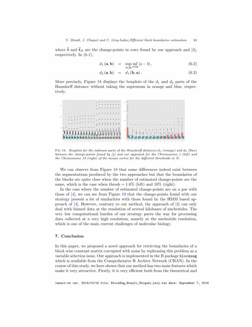
In order to compare our approach with the technique devised by [4], we dis-play in Figure 17 the number of change-points in rows found by our methodologyas a function of the threshold and a red line corresponding to the number ofchange-points found by [4]. Note that we did not display the change-points incolumns in order to save space since they are similar.
●
●
●
●
●
●
●
●
●
●
●
●
●
●
●
●
●
●
●
●
●
●
●
●
●
●
●
●
●
●
●
●
●
●
●
●
●
●
●
●
●
●
200
300
400
500
600
0.0 0.5 1.0 1.5 2.0
●
●
●
●
●
●
●
●
●
●
●
●
●
●
●
●
●
●
●
●
●
●
●
●
●
●
●
●
●
●
●
●
40
80
120
160
0 5 10 15
Fig 17. Number of change-points in rows found by our approach as a function of the threshold(in %) for the interaction matrices of Chromosome 1 (left) and Chromosome 19 (right) ofthe mouse cortex. The red line corresponds to the number of change-points found by [4].
We also compute the two parts of the Hausdorff distance for the change-pointsin rows which is defined by
d(tB , t
)= max
(d1
(tB , t
), d2
(tB , t
)), (6.1)
imsart-ss ver. 2014/10/16 file: BlockSeg_Brault_Chiquet_Levy.tex date: September 7, 2016
V. Brault, J. Chiquet and C. Levy-Leduc/Efficient block boundaries estimation 24
where t and tB are the change-points in rows found by our approach and [4],respectively. In (6.1),
d1 (a,b) = supb∈b
infa∈a|a− b| , (6.2)
d2 (a,b) = d1 (b,a) . (6.3)
More precisely, Figure 18 displays the boxplots of the d1 and d2 parts of theHausdorff distance without taking the supremum in orange and blue, respec-tively.
●
●●●●
●
●●
●
●
●
●
●
●●●●●●●
●
●●
●
●
●
●
●
●●●●●
●
●
●
●
●
●
●●
●●●●
●
●●
●
●
●
●
●
●●●●●
●
●
●
●
●
●
●
●●●
●
●
●
●●
●
●
●
●
●
●
●●●
●
●
●●●
●
●
●
●
●
●
●
●
●
●
●●
●
●●●
●
●
●
●
●
●
●●
●
●●
●●●
●
●
●
●
●
●
●
●●●
●
●●●●
●
●
●
●
●
●
●●
●
●●●
●●●
●
●
●
●
●
●
●
●
●
●●●●
●
●●●●
●
●
●
●
●
●
●●
●
●
●
●●●
●●●●
●
●
●
●
●
●
●
●
●
●●
●
●●
●
●●●●●
●
●
●
●
●
●
●●
●
●
●
●●●●●●●●
●
●
●
●
●
●
●
●
●
●●●
●
●●
●●
●●●●●
●
●
●
●
●
●
●
●
●●●●●●●●
●
●
●
●
●
●
●●
●
●●●●
●
●
●
●
●
●
●●
●
●
●
●
●
●
●●●
●
●
●
●
●
●
●
●
●
●
●
●
●
●
●
●
●
●
●●
●●
●
●
●
●
●
●
●●
●●
●●
●●
●
●
●
●
●
●●
●●●
●●●
●●
●
●
●
●
●
●●
●●
●●
●
●
●
●
●
●
●
●
●
●
●●
●●●
●●
●●
●
●
●
●
●
●
●
●
●●
●
●●
●
●
●
●
●
●
●
●
●
●
●
●●●
●
●
●
●
●
●
●
●
●●
●
●
●
●
●
●
●
●
●
●
●
●
●
●
●
●●
●
●
●
●
●
●
●
●
●●
●
●
●
●
●
●
●
●
●
●
●
●
●
●
●
●
●
●
●
●
●
●
●●
●
●
●
●
●
●
●
●
●
●
●
●
●
●
●
●
●
●
●
●
●
●
●●
●
●
●
●
●
●
●
●
●
●
●
●
●
●
●
●
●
●
●
●
●
●
●●
●
●
●
●
●
●
●
●
●
●
●
●
●
●
●
●
●
●
●
●
●
●●
●
●
●
●
●
●
●
●
●
●
●
●
●
●
●
●
●
●
●
●
●
●●
●●
●
●
●
●
●
●
●
●
●
●
●
●
●
●
●
●
●
●
●
●
●
●
●
●
●
●●
●●●●●
●●●●●
●●●
●●●●
●
●●
●●●
●
●
●●
●●●●●
●●
●
●●●●●●●
●●
●●●●
●
●●
●
●●●
●●●●●●●
●
●●
●●●●●●
●●●●●●●
●●●●
●●●●●●
●●●
●●●
●
●
●●
●●●●●
●
●
●●
●●●●●●●
●●●
●
●
●●●●
●●●
●
●●
●
●●
●●●●●
●
●
●●
●●●●
●●●
●
●
●●
●
●
●
●●
●
●
●●●●●●●●
●●●
●●●
●●
●
●
●
●
●●
●
●
●●●●●●●●●
●●●
●●●
●●
●
●●
●
●
●●●●
●
●
●●●●●●●
●●●
●●
●
●●
●●
●
●●●●
●
●
●●●●●●●
●●●
●●
●
●●
●●
●
●●●●
●
●
●●●
●●●●
●●●
●●
●
●●
●●
●
●●●●
●
●
●●●
●
●●●●●●●
●●
●
●
●●
●●
●
●●●
●
●
●
●
●
●●●●●●●
●●
●
●
●
●●●●●
●●●
●
●
●
●
●●●●●●
●●
●
●
●●●●●
●
●
●
●
●
●
●●●●●●●
●●
●
●
●●●●●
●
●
●
●
●
●●●●●●
●●
●
●
●●●●●
●
●
●
●
●
●●●●●●
●●
●
●
●●●●●
●
●
●
●
●
●●●●●●
●●
●
●
●●●●●
●
●
●
●
●●●●●●
●
●
●
●●●
●
●
●
●
●●●●●●●
●
●
●
●●●
●
●
●
●
●●●●●●
●
●
●
●●●
●
●
●
●●●●●●
●
●
●
●●●
●
●
●
0
100
200
300
0 0.1 0.2 0.3 0.4 0.5 0.6 0.7 0.8 0.9 1 1.1 1.2 1.3 1.4 1.5 1.6 1.7 1.8 1.9 2
●
●
●
●
●
●
●
●
●
●
●
●●
●
●
●●●●
●
●●●
●●●
●
●●●
●
●●●
●
●
●●●
●
●●●
●
●
●
●●
●
●
●
●
●
●
●
●
●
●
●
●
●
●
●
●
●
●
●
●
●●●
●
●●●
●
●
●
●
●
●
●
●
●
●
●
●
●
●
●
●
●
●
●
●
●
●●●●●
●
●
●
●●●● ●●●
●
●●● ●● ● ● ●
●●
●
●●
●
0
50
100
150
200
0 1 2 3 4 5 6 7 8 9 10 11 12 13 14 15
Fig 18. Boxplots for the infimum parts of the Hausdorff distances d1 (orange) and d2 (blue)between the change-points found by [4] and our approach for the Chromosome 1 (left) andthe Chromosome 19 (right) of the mouse cortex for the different thresholds in %.
We can observe from Figure 18 that some differences indeed exist betweenthe segmentations produced by the two approaches but that the boundaries ofthe blocks are quite close when the number of estimated change-points are thesame, which is the case when thresh = 1.8% (left) and 10% (right).
In the case where the number of estimated change-points are on a par withthose of [4], we can see from Figure 19 that the change-points found with ourstrategy present a lot of similarities with those found by the HMM based ap-proach of [4]. However, contrary to our method, the approach of [4] can onlydeal with binned data at the resolution of several kilobases of nucleotides. Thevery low computational burden of our strategy paves the way for processingdata collected at a very high resolution, namely at the nucleotide resolution,which is one of the main current challenges of molecular biology.
7. Conclusion
In this paper, we proposed a novel approach for retrieving the boundaries of ablock wise constant matrix corrupted with noise by rephrasing this problem as avariable selection issue. Our approach is implemented in the R package blocksegwhich is available from the Comprehensive R Archive Network (CRAN). In thecourse of this study, we have shown that our method has two main features whichmake it very attractive. Firstly, it is very efficient both from the theoretical and
imsart-ss ver. 2014/10/16 file: BlockSeg_Brault_Chiquet_Levy.tex date: September 7, 2016
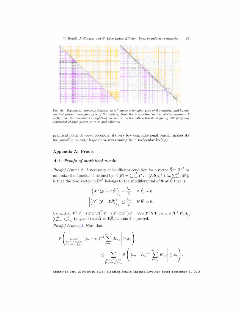
V. Brault, J. Chiquet and C. Levy-Leduc/Efficient block boundaries estimation 25
Fig 19. Topological domains detected by [4] (upper triangular part of the matrix) and by ourmethod (lower triangular part of the matrix) from the interaction matrix of Chromosome 1(left) and Chromosome 19 (right) of the mouse cortex with a threshold giving 232 (resp 85)estimated change-points in rows and columns.
practical point of view. Secondly, its very low computational burden makes itsuse possible on very large data sets coming from molecular biology.
Appendix A: Proofs
A.1. Proofs of statistical results
Proofof Lemma 2. A necessary and sufficient condition for a vector B in Rn2
to
minimize the function Φ defined by: Φ(B) =∑n2
i=1(Yi− (XB)i)2 +λn
∑n2
i=1 |Bi|,is that the zero vector in Rn2
belongs to the subdifferential of Φ at B that is:(X>(Y − XB)
)j
=λn2, if Bj 6= 0,∣∣∣∣(X>(Y − XB)
)j
∣∣∣∣ ≤ λn2, if Bj = 0.
Using that X>Y = (T⊗T)>Y = (T>⊗T>)Y = Vec(T>YT), where (T>YT)i,j =∑n
k=i
∑n`=j Yk,`, and that U = XB, Lemma 2 is proved.
Proofof Lemma 3. Note that
P
max1≤rn<sn≤n
|rn−sn|≥vn
∣∣∣∣∣∣(sn − rn)−1sn−1∑j=rn
En,j
∣∣∣∣∣∣ ≥ xn
≤∑
1≤rn<sn≤n
|rn−sn|≥vn
P
∣∣∣∣∣∣(sn − rn)−1sn−1∑j=rn
En,j
∣∣∣∣∣∣ ≥ xn .
imsart-ss ver. 2014/10/16 file: BlockSeg_Brault_Chiquet_Levy.tex date: September 7, 2016
V. Brault, J. Chiquet and C. Levy-Leduc/Efficient block boundaries estimation 26
By (A1) and the Markov inequality, we get that for all positive η,
P
(sn − rn)−1sn−1∑j=rn
En,j ≥ xn
≤ exp[−η(sn − rn)xn](E(exp(ηE1,1)))sn−rn
≤ exp[−η(sn − rn)xn + βη2(sn − rn)].
By taking η = xn/(2β), we get that
P
(sn − rn)−1sn−1∑j=rn
En,j ≥ xn
≤ exp[−x2n(sn − rn)/(4β)].
Since the same result is valid for −En,j , we get that
P
max1≤rn<sn≤n
|rn−sn|≥vn
∣∣∣∣∣∣(sn − rn)−1sn−1∑j=rn
En,j
∣∣∣∣∣∣ ≥ xn ≤ 2n2 exp[−x2nvn/(4β)],
which concludes the proof of Lemma 3.
Proofof Proposition 1. Since
P({
max1≤k≤K?
1
∣∣t1,k − t?1,k∣∣ > nδn
}∪{
max1≤k≤K?
2
∣∣t2,k − t?2,k∣∣ > nδn
})≤ P
(max
1≤k≤K?1
∣∣t1,k − t?1,k∣∣ > nδn
)+ P
(max
1≤k≤K?2
∣∣t2,k − t?2,k∣∣ > nδn
), (A.1)
it is enough to prove that both terms in (A.1) tend to zero for proving (2.6). Weshall only prove that the second term in the rhs of (A.1) tends to zero, the proofbeing the same for the first term. Since P(max1≤k≤K?
2|t2,k − t?2,k| > nδn) ≤∑K?
2
k=1 P(|t2,k − t?2,k| > nδn), it is enough to prove that for all k in {1, . . . ,K?2},
P(An,k)→ 0, where An,k = {|t2,k − t?2,k| > nδn}. Let Cn be defined by
Cn =
{max
1≤k≤K?2
|t2,k − t?2,k| < I?min,2/2
}. (A.2)
It is enough to prove that, for all k in {1, . . . ,K?2}, P(An,k∩Cn) and P(An,k∩Cn)
tend to 0, as n tends to infinity.Let us first prove that for all k in {1, . . . ,K?
2}, P(An,k ∩ Cn) → 0. Observethat (A.2) implies that t?2,k−1 < t2,k < t?2,k+1, for all k in {1, . . . ,K?
2}. For a
given k, let us assume that t2,k ≤ t?2,k. Applying (2.7) and (2.8) with rj +1 = n,
qj + 1 = t2,k on the one hand and rj + 1 = n, qj + 1 = t?2,k on the other hand,we get that ∣∣∣∣∣∣
t?2,k−1∑j=t2,k
Yn,j −t?2,k−1∑j=t2,k
Un,j
∣∣∣∣∣∣ ≤ λn.imsart-ss ver. 2014/10/16 file: BlockSeg_Brault_Chiquet_Levy.tex date: September 7, 2016
V. Brault, J. Chiquet and C. Levy-Leduc/Efficient block boundaries estimation 27
Hence using (2.1), the notation: E([a, b]; [c, d]) =∑bi=a
∑dj=cEi,j and the defi-
nition of U given by Lemma 2, we obtain that∣∣∣(t?2,k − t2,k)(µ?K?1+1,k − µK?
1+1,k+1) + E(n; [t2,k, t?2,k − 1])
∣∣∣ ≤ λn,which can be rewritten as follows∣∣∣(t?2,k − t2,k)(µ?K?
1+1,k − µ?K?1+1,k+1) + (t?2,k − t2,k)(µ?K?
1+1,k+1 − µK?1+1,k+1)
+E(n; [t2,k, t?2,k − 1])
∣∣ ≤ λn.Thus,
P(An,k ∩ Cn) ≤ P(λn/(nδn) ≥ |µ?K?1+1,k − µ?K?
1+1,k+1|/3)
+ P({|µ?K?1+1,k − µK?
1+1,k+1| ≥ |µ?K?1+1,k − µ?K?
1+1,k+1|/3} ∩ Cn)
+ P({|E(n; [t2,k, t?2,k − 1])|/|t?2,k − t2,k| ≥ |µ?K?
1+1,k − µ?K?1+1,k+1|/3} ∩An,k).
(A.3)
The first term in the rhs of (A.3) tends to 0 by (A2). By Lemma 3 with xn =J?min/3, vn = nδn and (A3) the third term in the rhs of (A.3) tends to 0.Applying Lemma 2 with rj+1 = n, qj+1 = t2,k on the one hand and rj+1 = n,qj + 1 = (t?2,k + t?2,k+1)/2 on the other hand, we get that∣∣∣∣∣∣
(t?2,k+t?2,k+1)/2−1∑j=t?2,k
Yn,j −(t?2,k+t
?2,k+1)/2−1∑j=t?2,k
Un,j
∣∣∣∣∣∣ ≤ λn.Since t2,k ≤ t?2,k, Un,j = µK?
1+1,k+1 within the interval [t?2,k, (t?2,k+ t?2,k+1)/2−1]
and we get that
(t?2,k+1−t?2,k)|µ?K?1+1,k+1−µK?
1+1,k+1|/2 ≤ λn+|E(n, |[t?2,k, (t?2,k+t?2,k+1)/2−1])|.
Therefore the second term in the rhs of (A.3) can be bounded by
P(λn ≥ (t?2,k+1 − t?2,k)|µ?K?
1+1,k − µ?K?1+1,k+1|/12
)+ P
((t?2,k+1 − t?2,k)−1
∣∣E(n, , |[t?2,k, (t?2,k + t?2,k+1)/2− 1])∣∣
≥ |µ?K?1+1,k − µ?K?
1+1,k+1|/6)
By Lemma 3 and (A2), (A3) and (A4), we get that both terms tend to zero asn tends to infinity. We thus get that P(An,k ∩ Cn)→ 0, as n tends to infinity.
Let us now prove that P(An,k ∩Cn) tend to 0, as n tends to infinity. Observethat
P(An,k ∩ Cn) = P(An,k ∩D(`)n ) + P(An,k ∩D(m)
n ) + P(An,k ∩D(r)n ),
imsart-ss ver. 2014/10/16 file: BlockSeg_Brault_Chiquet_Levy.tex date: September 7, 2016
V. Brault, J. Chiquet and C. Levy-Leduc/Efficient block boundaries estimation 28
where
D(`)n =
{∃p ∈ {1, . . . ,K?}, t2,p ≤ t?2,p−1
}∩ Cn,
D(m)n =
{∀k ∈ {1, . . . ,K?}, t?2,k−1 < t2,k < t?2,k+1
}∩ Cn,
D(r)n =
{∃p ∈ {1, . . . ,K?}, t2,p ≥ t?2,p+1
}∩ Cn.
Using the same arguments as those used for proving that P(An,k ∩Cn)→ 0, we
can prove that P(An,k ∩ D(m)n ) → 0, as n tends to infinity. Let us now prove
that P(An,k ∩D(`)n )→ 0. Note that
P(D(`)n ) ≤
K?2−1∑k=1
P({t?2,k − t2,k > I?min/2} ∩ {t2,k+1 − t?2,k > I?min/2})
+P(t?2,K?2− t2,K?
2> I?min/2). (A.4)
Applying (2.7) and (2.8) with rj + 1 = n, qj + 1 = t2,k on the one hand andrj + 1 = n, qj + 1 = t?2,k on the other hand, we get that∣∣∣∣∣∣
t?2,k−1∑j=t2,k
Yn,j −t?2,k−1∑j=t2,k
Un,j
∣∣∣∣∣∣ ≤ λn.Thus,
P({t?2,k − t2,k > I?min/2} ∩ {t2,k+1 − t?2,k > I?min/2})≤ P(λn/(nδn) ≥ |µ?K?
1+1,k − µ?K?1+1,k+1|/3)
+P({|µ?K?1+1,k − µK?
1+1,k+1| ≥ |µ?K?1+1,k − µ?K?
1+1,k+1|/3}
∩{t2,k+1 − t?2,k > I?min/2})+P({|E(n; [t2,k, t
?2,k − 1])|/(t?2,k − t2,k) ≥ |µ?K?
1+1,k − µ?K?1+1,k+1|/3}
∩{t?2,k − t2,k > I?min/2}). (A.5)
Using the same arguments as previously we get that the first and the third termin the rhs of (A.5) tend to zero as n tends to infinity. Let us now focus onthe second term of the rhs of (A.5). Applying (2.7) and (2.8) with rj + 1 = n,qj + 1 = t2,k+1 on the one hand and rj + 1 = n, qj + 1 = t?2,k on the other hand,we get that ∣∣∣∣∣∣
t2,k+1−1∑j=t?2,k
Yn,j −t2,k+1−1∑j=t?2,k
Un,j
∣∣∣∣∣∣ ≤ λn.Hence,
|(µ?K?1+1,k − µK?
1+1,k+1)(t2,k+1 − t?2,k) + E(n, [t?2,k; t2,k+1 − 1])| ≤ λn.
imsart-ss ver. 2014/10/16 file: BlockSeg_Brault_Chiquet_Levy.tex date: September 7, 2016

V. Brault, J. Chiquet and C. Levy-Leduc/Efficient block boundaries estimation 29
The second term of the rhs of (A.5) is thus bounded by
P({λn(t2,k+1 − t?2,k)−1 ≥ |µ?K?1+1,k − µ?K?
1+1,k+1|/6}
∩{t2,k+1 − t?2,k > I?min/2})+P({(t2,k+1 − t?2,k)−1|E(n, [t?2,k; t2,k+1 − 1])| ≥ |µ?K?
1+1,k − µ?K?1+1,k+1|/6}
∩{t2,k+1 − t?2,k > I?min/2}),
which tend to zero by Lemma 3, (A2), (A3) and (A4). It is thus proved thatthe first term in the rhs of (A.4) tends to zero as n tends to infinity. The samearguments can be used for addressing the second term in the rhs of (A.4) sincet2,K?
2+1 = n and hence t2,K?2+1 − t?2,K?
2> I?min/2.
Using similar arguments, we can prove that P(An,k ∩D(r)n )→ 0, which con-
cludes the proof of Proposition 1.
A.2. Proofs of computational lemmas
Proofof Lemma 4.. Consider Xv for instance (the same reasoning applies forX>v): we have Xv = (T ⊗ T)v = Vec(TVT>) where V is the n × n matrixsuch that Vec(V) = v. Because of its triangular structure, T operates as acumulative sum operator on the columns of V. Hence, the computations for thejth column is done by induction in n operations. The total cost for the n columnsof TV is thus n2. Similarly, right multiplying a matrix by T> boils down toperform cumulative sums over the rows. The final cost for Xv = Vec(TVT>)is thus 2n2 in case of a dense matrix V, and possibly less when V is sparse.
Proof of Lemma 5. Let A = {a1, . . . , aK}, then(X>X
)A,A = (T⊗T)
>•,A(T⊗T)•,A, (A.6)
where (T ⊗ T)•,A (resp. (T⊗T)>•,A) denotes the columns (resp. the rows) of
T ⊗ T lying in A. For j in A, let us consider the Euclidean division of j − 1by n given by: (j − 1) = nqj + rj , then (T⊗T)•,j = T•,qj+1 ⊗T•,rj+1. Hence,(T⊗T)•,A is a n2 ×K matrix defined by:
(T⊗T)•,A =[T•,qa1+1 ⊗T•,ra1+1 ; T•,qa2+1 ⊗T•,ra2+1 ; . . . ; T•,qaK+1 ⊗T•,raK+1
].
Thus,
(T⊗T)•,A = T•,QA ∗T•,RA , where QA = {qa1 + 1, . . . , qaK + 1},RA = {ra1 + 1, . . . , raK + 1}
and ∗ denotes the Khatri-Rao product, which is defined as follows for two n×nmatrices A and B
A ∗B = [a1 ⊗ b1; a2 ⊗ b2; . . . an ⊗ bn] ,
imsart-ss ver. 2014/10/16 file: BlockSeg_Brault_Chiquet_Levy.tex date: September 7, 2016
V. Brault, J. Chiquet and C. Levy-Leduc/Efficient block boundaries estimation 30
where the ai (resp. bi) are the columns of A (resp. B). Using (25) of Theorem 2in [13], we get that
(T⊗T)>•,A(T⊗T)•,A =
(T>•,QAT•,QA
)◦(T>•,RAT•,RA
),
where ◦ denotes the Hadamard or entry-wise product. Observe that by definitionof T, (T>•,QAT•,QA)k,` = n− (qak ∨ qa`) and (T>•,RAT•,RA)k,` = n− (rak ∨ ra`).By (A.6),
(X>X
)A,A is a Gram matrix which is positive and definite since the
vectors T•,qa1+1⊗ T•,ra1+1
, T•,qa2+1⊗ T•,ra2+1
, . . . , T•,qaK+1⊗ T•,raK+1
arelinearly independent.
Proofof Lemma 6.. The operations of adding/removing a column to a Choleskyfactorization are classical and well treated in books of numerical analysis, seee.g. [7]. An advantage of our settings is that there is no additional computationalcost for computing X>X�j when entering a new variable j thanks to the closed-form expression (3.1).
Acknowledgements
V. Brault would like to thank the French National Research Agency ANR, whichpartly supported this research through the ABS4NGS project (ANR-11-BINF-0001-06).
References
[1] Bach, F., R. Jenatton, J. Mairal, and G. Obozinski (2012). Optimiza-tion with sparsity-inducing penalties. Foundations and Trends R© in MachineLearning 4(1), 1–106.
[2] Bellman, R. (1961). On the approximation of curves by line segments usingdynamic programming. Commun. ACM 4(6), 284–286.
[3] Breiman, L., J. H. Friedman, R. A. Olshen, and C. J. Stone (1984).Classification and Regression Trees. Statistics/Probability Series. Belmont,California, U.S.A.: Wadsworth Publishing Company.
[4] Dixon, J. R., S. Selvaraj, F. Yue, A. Kim, Y. Li, Y. Shen, M. Hu, J. S. Liu,and B. Ren (2012). Topological domains in mammalian genomes identifiedby analysis of chromatin interactions. Nature 485(7398), 376–380.
[5] Efron, B., T. Hastie, I. Johnstone, R. Tibshirani, et al. (2004). Least angleregression. The Annals of statistics 32(2), 407–499.
[6] Fisher, W. D. (1958). On grouping for maximum homogeneity. Journal ofthe American Statistical Association 53(284), 789–798.
[7] Golub, G. H. and C. F. Van Loan (2012). Matrix computations. JHU Press.3rd edition.
[8] Harchaoui, Z. and C. Levy-Leduc (2010). Multiple change-point estima-tion with a total variation penalty. Journal of the American StatisticalAssociation 105(492), 1480–1493.
imsart-ss ver. 2014/10/16 file: BlockSeg_Brault_Chiquet_Levy.tex date: September 7, 2016
V. Brault, J. Chiquet and C. Levy-Leduc/Efficient block boundaries estimation 31
[9] Hoefling, H. (2010). A path algorithm for the fused lasso signal approxima-tor. J. Comput. Graph. Statist. 19(4), 984–1006.
[10] Kay, S. (1993). Fundamentals of statistical signal processing: detectiontheory. Prentice-Hall, Inc.
[11] Levy-Leduc, C., M. Delattre, T. Mary-Huard, and S. Robin (2014). Two-dimensional segmentation for analyzing hi-c data. Bioinformatics 30(17),i386–i392.
[12] Lieberman-Aiden, E., N. L. Van Berkum, L. Williams, M. Imakaev,T. Ragoczy, A. Telling, I. Amit, B. R. Lajoie, P. J. Sabo, M. O. Dorschner,et al. (2009). Comprehensive mapping of long-range interactions reveals fold-ing principles of the human genome. science 326(5950), 289–293.
[13] Liu, S. and G. Trenkler (2008). Hadamard, khatri-rao, kronecker and othermatrix products. Int. J. Inform. Syst. Sci. 4, 160–177.
[14] Maidstone, R., T. Hocking, G. Rigaill, and P. Fearnhead (2016). On optimalmultiple changepoint algorithms for large data. Statistics and Computing, 1–15.
[15] Meinshausen, N. and P. Buhlmann (2010). Stability selection. Journal ofthe Royal Statistical Society: Series B (Statistical Methodology) 72(4), 417–473.
[16] Osborne, M. R., B. Presnell, and B. A. Turlach (2000). A new approachto variable selection in least squares problems. IMA journal of numericalanalysis 20(3), 389–403.
[17] R Core Team (2015). R: A Language and Environment for StatisticalComputing. Vienna, Austria: R Foundation for Statistical Computing.
[18] Sanderson, C. (2010). Armadillo: An open source C++ linear algebra li-brary for fast prototyping and computationally intensive experiments. Tech-nical report, NICTA.
[19] Tibshirani, R. J. and J. Taylor (2011). The solution path of the generalizedlasso. Ann. Statist. 39(3), 1335–1371.
[20] Vert, J.-P. and K. Bleakley (2010). Fast detection of multiple change-pointsshared by many signals using group lars. In Advances in Neural InformationProcessing Systems, pp. 2343–2351.
imsart-ss ver. 2014/10/16 file: BlockSeg_Brault_Chiquet_Levy.tex date: September 7, 2016


