Efficient computation of multivariabletransfer function dominant poles using

subspace acceleration

by

Joost Rommes and Nelson Martins

Universiteit-Utrecht*

Departmentof Mathematics

Preprint

nr. 1344

January, 2006

Efficient computation of multivariable transfer function

dominant poles using subspace acceleration

Joost Rommes∗ and Nelson Martins†

January, 2006

Abstract

This paper describes a new algorithm to compute the dominant poles of a high-ordermulti-input multi-output (MIMO) transfer function. The algorithm, called the SubspaceAccelerated MIMO Dominant Pole Algorithm (SAMDP), is able to compute the full set ofdominant poles efficiently. SAMDP can be used to produce good modal equivalents automat-ically. The general algorithm is robust, applicable to both square and non-square transferfunction matrices, and can easily be tuned to suit different practical system needs.

1 Introduction

Current model reduction techniques for power system stability analysis and controller design [1–5]produce good results but are not applicable to large scale problems. If only a small part of thesystem pole spectrum is controllable-observable for the transfer function, a low-cost alternative forlarge-scale systems is modal model reduction. Modal reduction approximates the transfer functionby a modal equivalent that is computed from the dominant poles and their corresponding residues.To produce a good modal equivalent, specialized eigensolution methods are needed. An algorithmthat automatically and efficiently computes the full set of dominant poles of a scalar transferfunction was presented recently [6], but existing methods for multi-input multi-output (MIMO)transfer functions [7] are not capable enough to produce good modal equivalents automatically.A survey on model reduction methods employing either singular value decompositions or momentmatching based methods is found in [8, 9]. An introduction on modal model reduction on statespace models can be found in [10], while [11] describes a possible enhancement to modal modelreduction.

In this article, a new extension of the Subspace Accelarated Dominant Pole Algorithm (SADPA)[6] will be proposed: Subspace Accelerated MIMO Dominant Pole Algorithm (SAMDP). TheSADPA is a generalization of the Dominant Pole Algorithm [12], that automatically computes ahigh quality modal equivalent of a transfer function. The SAMDP can also be seen as a gener-alization of the MIMO Dominant Pole algorithm [7]. SAMDP computes the dominant poles andcorresponding residue matrices one by one by selecting the most dominant approximation everyiteration. This approach leads to a faster, more robust and more flexible algorithm. To avoidrepeated computation of the same dominant poles, a deflation strategy is used. The SAMDPdirectly operates on implicit state space systems, also known as descriptor systems, which arevery sparse in practical power system applications.

The article is organized as follows. Section 2 summarizes some well known properties ofMIMO transfer functions and formulates the problem of computing the dominant poles of a MIMOtransfer function. Section 3 describes the new SAMDP algorithm. In section 4, numerical aspectsconcerning practical implementations of SAMDP are discussed. Extensive numerical results arepresented in 5. Section 6 concludes.

∗Joost Rommes is with Mathematical Institute, Utrecht University, P.O.Box 80100, 3508 TA Utrecht, TheNetherlands (rommes@math.uu.nl).

†Nelson Martins is with CEPEL, P.O.Box 68007 - Rio de Janeiro, RJ - 20001 - 970, Brazil (nelson@cepel.br).

1

2 MIMO transfer functions, sigma plots and dominant poles

For a multi-input multi-output (MIMO) system{x(t) = Ax(t) + Bu(t)y(t) = CT x(t) + Du(t), (1)

where A ∈ Rn×n, B ∈ Rn×m, C ∈ Rn×p, x(t) ∈ Rn, u(t) ∈ Rm, y(t) ∈ Rp and D ∈ Rp×m, thetransfer function H(s) : C −→ Cp×m is defined as

H(s) = CT (sI −A)−1B + D, (2)

where I ∈ Rn×n is the identity matrix and s ∈ C. Without loss of generality, D = 0 in thefollowing.

It is well known that the transfer function of single-input single-output system is defined bya complex number for any frequency. For a MIMO system, the transfer function is a p × mmatrix and hence does not have a unique gain for a given frequency. The SISO concept of asingle transfer function gain must be replaced by a range of gains that have an upper bound fornon-square matrices H(s), and both upper and lower bounds for square matrices H(s). Denotingthe smallest and largest singular values [13] of H(jω) by σmin(ω) and σmax(ω), it follows for squareH(s) that

σmin(jω) ≤ ||H(jω)u(jω)||2||u(jω)||2

≤ σmax(jω),

ie. for a given frequency ω, the gain of a MIMO transfer function is between the smallest andlargest singular value of H(jω), which are also called the smallest and largest principal gains [14].For non-square transfer functions H(s), only the upper bound holds. Plots of the smallest andlargest principal gains against frequency, also known as sigma plots, are used in the robust controldesign and analysis of MIMO systems [14].

Let the eigenvalues (poles) of A and the corresponding right and left eigenvectors be given bythe triplets (λj ,xj ,yj), and let the right and left eigenvectors be scaled so that y∗jxj = 1. Notethat y∗jxk = 0 for j 6= k. The transfer function H(s) can be expressed as a sum of residue matricesRj ∈ Cp×m over first order poles [15]:

H(s) =n∑

j=1

Rj

s− λj,

where the residue matrices Rj areRj = (CT xj)(y∗j B).

A pole λj that corresponds to a residue Rj with large norm ||Rj ||2 = σmax(Rj) is called adominant pole, i.e. a pole that is well observable and controllable in the transfer function. Thiscan also be observed from the corresponding σmax-plot of H(s), where peaks occur at frequenciesclose to the imaginary parts of the dominant poles of H(s). An approximation of H(s) thatconsists of k < n terms with ||Rj ||2 above some value, determines the effective transfer functionbehaviour [16] and will be referred to as transfer function modal equivalent:

Hk(s) =k∑

j=1

Rj

s− λj,

Because a residue matrix Rj is the product of a column vector and a row vector, it is of unit rank.Therefore at least min(m, p) different poles are needed to obtain a modal equivalent with nonzeroσmin(ω) plot [7, 17].

The problem of concern can now be formulated as: Given a MIMO linear, time invariant,dynamical system (A,B,C, D), compute k � n dominant poles λj and the corresponding rightand left eigenvectors xj and yj .

2

3 Subspace Accelerated MIMO Dominant Pole Algorithm(SAMDP)

The subspace accelerated MIMO dominant pole algorithm (SAMDP) is based on the dominantpole algorithm (DPA) [12], the subspace accelerated DPA (SADPA) [6] and the MIMO dominantpole algorithm (MDP) [7]. First, a Newton scheme will be derived for computing the dominantpoles of a MIMO transfer function. Then, the SAMDP will be formulated as an acceleratedNewton scheme, using the same improvements that were used in the robust SADPA algorithm.

All algorithms are described as directly operating on the state-space model. The practicalimplementations (see section 4.1) operate on the sparse descriptor system model, which is theunreduced Jacobian for the power system stability problem, analized in the examples of this paper(see section 5).

3.1 Newton scheme for computing dominant poles

The dominant poles of a MIMO transfer function H(s) = CT (sI − A)−1B are those s ∈ C forwhich σmax(H(s)) → ∞. For square transfer functions (m = p), there is an equivalent criterion:the dominant poles are those s ∈ C for which λmin(H−1(s)) → 0. In the following it will beassumed that m = p; for general MIMO transfer functions, see 4.3.

The Newton method can be used to find the s ∈ C for which the objective function

f : C −→ C : s 7−→ λmin((CT (sI −A)−1B)−1) (3)

is zero. Let (µ(s),u(s),v(s)) be an eigentriplet of H−1(s) ∈ Cm×m, ie. H−1(s)u(s) = µ(s)u(s)and v∗(s)H−1(s) = µ(s)v∗(s), with v∗(s)u(s) = 1. The derivative of µ(s) is given by [18]

dµ

ds(s) = v∗(s)

dH−1

ds(s)u(s), (4)

where

dH−1

ds(s) = −H−1(s)

dH

ds(s)H−1(s)

= H−1(s)CT (sI −A)−2BH−1(s). (5)

Note that it is assumed that H−1(s) has distinct eigenvalues and that the function that selectsµmin(s) has derivative 1. Substituting (5) in (4), it follows that

dµ

ds(s) = v∗(s)H−1(s)CT (sI −A)−2BH−1(s)u(s)

= µ2(s)v∗(s)CT (sI −A)−2Bu(s).

The Newton scheme then becomes

sk+1 = sk − f(sk)f ′(sk)

= sk − µmin

µ2minv∗CT (skI −A)−2Bu

= sk − 1µmin

1v∗CT (skI −A)−2Bu

,

where (µmin,u,v) = (µmin(sk),umin(sk),v∗min(sk)) is the eigentriplet of H−1(sk) correspondingto λmin(H−1(sk)). An algorithm, very similar to the DPA algorithm [12], for the computation ofsingle dominant pole of a MIMO transfer function using the above Newton scheme, is shown inAlg. 1. In the neighborhood of a solution, Alg. 1 converges quadratically.

3

Algorithm 1 A MIMO Dominant Pole Algorithm.INPUT: System (A,B,C), initial pole estimate s1

OUTPUT: Dominant pole λ and corresponding right and left eigenvectors x and y.1: Set k = 12: while not converged do3: Compute eigentriplet (µmin,u,v) of H−1(sk)4: Solve x ∈ Cn from

(skI −A)x = Bu

5: Solve y ∈ Cn from(skI −A)∗y = Cv

6: Compute the new pole estimate

sk+1 = sk −1

µmin

1y∗x

7: The pole λ = sk+1 has converged if

||Ax− sk+1x||2 < ε

for some ε � 18: Set k = k + 19: end while

3.2 SAMDP as an accelerated Newton scheme

The three strategies that are used for SADPA [6], are also used to make SAMDP, a generalizationof Alg. 1: subspace acceleration, selection of most dominant approximation and deflation. Aglobal overview of the SAMDP is shown in Alg. 2. Each of the three strategies is explained in thefollowing paragraphs.

3.2.1 Subspace acceleration

The approximations x and y that are computed in steps 4 and 5 of Alg. 1 are kept in orthogonalsearch spaces X and Y , using modified Gram-Schmidt (MGS) [13]. These search spaces growevery iteration and will contain better approximations (see step 6 and 7 of Alg. 2).

3.2.2 Selection strategy

Every iteration a new pole estimate sk must be chosen. There are several strategies (see [6] andsection 4.2). Here the most natural choice is to select the triplet (λj , xj , yj) with largest residuenorm ||Rj ||2. SAMDP continues with sk+1 = λj . See Alg. 3.

Algorithm 3 (Λ, X, Y ) = Sort(Λ, X, Y, B, C)

INPUT: Λ ∈ Cn, X, Y ∈ Cn×k, B ∈ Rn×p,C ∈ Rn×m

OUTPUT: Λ ∈ Cn, X, Y ∈ Cn×k with λ1 the pole with largest residue matrix norm and x1 andy1 the corresponding approximate right and left eigenvectors.

1: Compute residue matrices Ri = (CT xi)(y∗i B)2: Sort Λ, X, Y in decreasing ||Ri||2 order

3.2.3 Deflation

An eigentriplet (λj , xj , yj) has converged if ||Axj − λjxj ||2 is smaller than some tolerance ε. Ifmore than one eigentriplet is wanted, repeated computation of already converged eigentriplets

4

Algorithm 2 Subspace Accelerated MDP Algorithm.INPUT: System (A,B,C), initial pole estimate s1 and the number of wanted poles pmax

OUTPUT: Dominant pole triplets (λi, ri, li), i = 1, . . . , pmax

1: k = 1, pfound = 0, X = Y = Λ = R = L = []2: while pfound < pmax do3: Compute eigentriplet (µmin,u,v) of H−1(sk)4: Solve x ∈ Cn from

(skI −A)x = Bu

5: Solve y ∈ Cn from(skI −A)∗y = Cv

6: X = Expand(X, R,L,x) {Alg. 4}7: Y = Expand(Y,L,R,y) {Alg. 4}8: Compute G = Y ∗X and T = Y ∗AX9: Compute eigentriplets of (T,G):

(λi, xi, yi), i = 1, . . . , k

10: Compute approximate eigentriplets of A as

(λi = λi, xi = Xxi, yi = Y yi), i = 1, . . . , k

11: Λ = [λ1, . . . , λk]12: X = [x1, . . . , xk]13: Y = [y1, . . . , yk]14: (Λ, X, Y ) = Sort(Λ, X, Y , B,C) {Alg. 3}15: if ||Ax1 − λ1x1||2 < ε then16: (Λ, R, L, X, Y ) =

Deflate(λ1, x1, y1,Λ, R, L, X2:k, Y2:k) {Alg. 5}17: pfound = pfound + 118: Set λ1 = λ2

19: end if20: Set k = k + 121: Set the new pole estimate sk+1 = λ1

22: end while

5

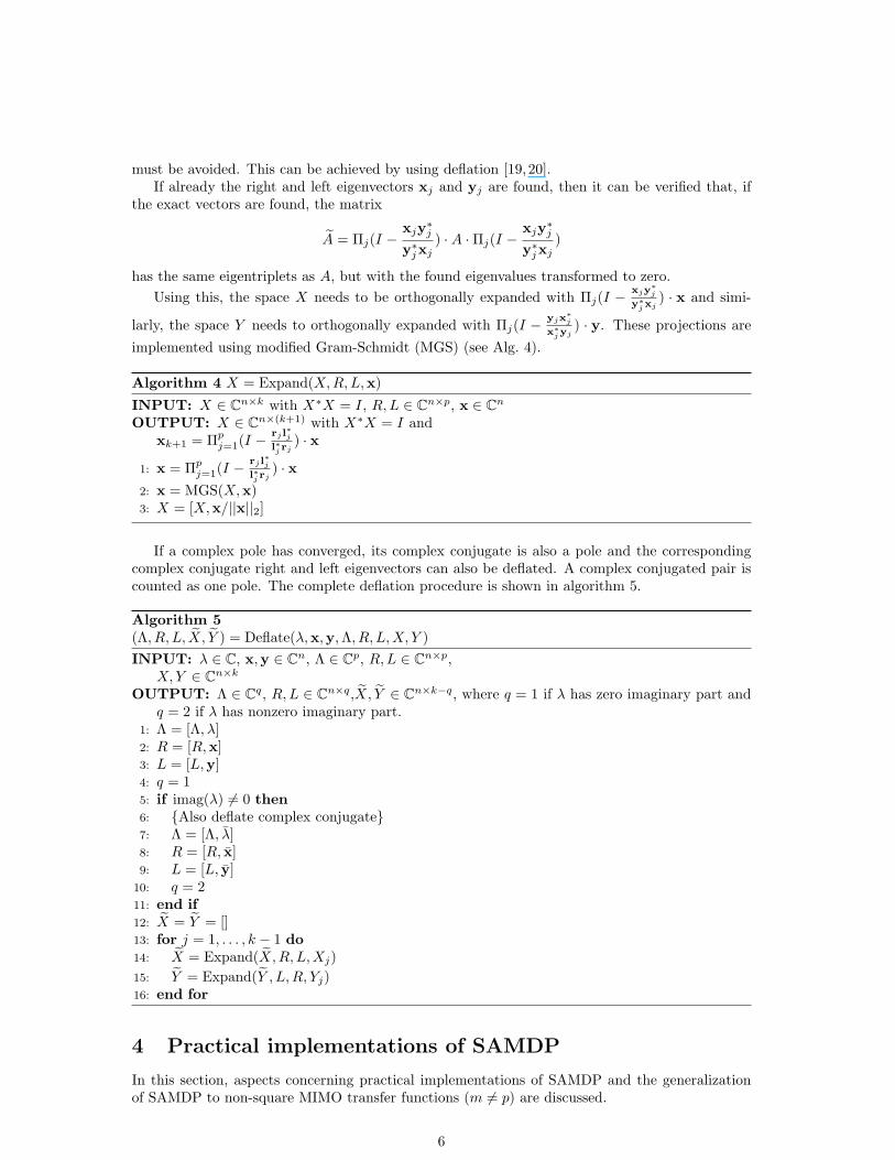
must be avoided. This can be achieved by using deflation [19,20].If already the right and left eigenvectors xj and yj are found, then it can be verified that, if

the exact vectors are found, the matrix

A = Πj(I −xjy∗jy∗jxj

) ·A ·Πj(I −xjy∗jy∗jxj

)

has the same eigentriplets as A, but with the found eigenvalues transformed to zero.Using this, the space X needs to be orthogonally expanded with Πj(I −

xjy∗j

y∗j xj) · x and simi-

larly, the space Y needs to orthogonally expanded with Πj(I −yjx

∗j

x∗j yj) · y. These projections are

implemented using modified Gram-Schmidt (MGS) (see Alg. 4).

Algorithm 4 X = Expand(X, R,L,x)

INPUT: X ∈ Cn×k with X∗X = I, R,L ∈ Cn×p, x ∈ Cn

OUTPUT: X ∈ Cn×(k+1) with X∗X = I andxk+1 = Πp

j=1(I −rj l

∗j

l∗j rj) · x

1: x = Πpj=1(I −

rj l∗j

l∗j rj) · x

2: x = MGS(X,x)3: X = [X,x/||x||2]

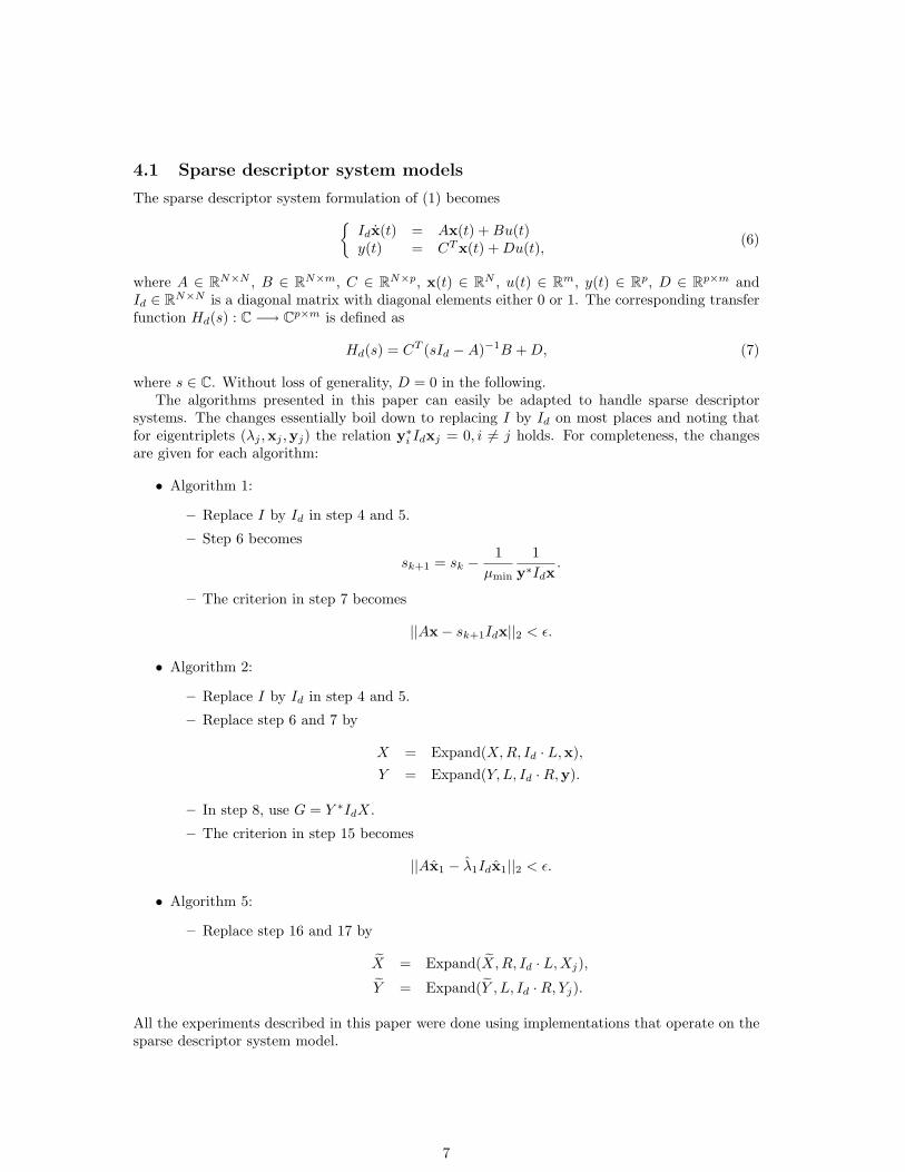
If a complex pole has converged, its complex conjugate is also a pole and the correspondingcomplex conjugate right and left eigenvectors can also be deflated. A complex conjugated pair iscounted as one pole. The complete deflation procedure is shown in algorithm 5.

Algorithm 5(Λ, R, L, X, Y ) = Deflate(λ,x,y,Λ, R, L, X, Y )INPUT: λ ∈ C, x,y ∈ Cn, Λ ∈ Cp, R,L ∈ Cn×p,

X, Y ∈ Cn×k

OUTPUT: Λ ∈ Cq, R,L ∈ Cn×q,X, Y ∈ Cn×k−q, where q = 1 if λ has zero imaginary part andq = 2 if λ has nonzero imaginary part.

1: Λ = [Λ, λ]2: R = [R,x]3: L = [L,y]4: q = 15: if imag(λ) 6= 0 then6: {Also deflate complex conjugate}7: Λ = [Λ, λ]8: R = [R, x]9: L = [L, y]

10: q = 211: end if12: X = Y = []13: for j = 1, . . . , k − 1 do14: X = Expand(X, R, L, Xj)15: Y = Expand(Y , L,R, Yj)16: end for

4 Practical implementations of SAMDP

In this section, aspects concerning practical implementations of SAMDP and the generalizationof SAMDP to non-square MIMO transfer functions (m 6= p) are discussed.

6

4.1 Sparse descriptor system models

The sparse descriptor system formulation of (1) becomes{Idx(t) = Ax(t) + Bu(t)y(t) = CT x(t) + Du(t), (6)

where A ∈ RN×N , B ∈ RN×m, C ∈ RN×p, x(t) ∈ RN , u(t) ∈ Rm, y(t) ∈ Rp, D ∈ Rp×m andId ∈ RN×N is a diagonal matrix with diagonal elements either 0 or 1. The corresponding transferfunction Hd(s) : C −→ Cp×m is defined as

Hd(s) = CT (sId −A)−1B + D, (7)

where s ∈ C. Without loss of generality, D = 0 in the following.The algorithms presented in this paper can easily be adapted to handle sparse descriptor

systems. The changes essentially boil down to replacing I by Id on most places and noting thatfor eigentriplets (λj ,xj ,yj) the relation y∗i Idxj = 0, i 6= j holds. For completeness, the changesare given for each algorithm:

• Algorithm 1:

– Replace I by Id in step 4 and 5.

– Step 6 becomes

sk+1 = sk −1

µmin

1y∗Idx

.

– The criterion in step 7 becomes

||Ax− sk+1Idx||2 < ε.

• Algorithm 2:

– Replace I by Id in step 4 and 5.

– Replace step 6 and 7 by

X = Expand(X, R, Id · L,x),Y = Expand(Y, L, Id ·R,y).

– In step 8, use G = Y ∗IdX.

– The criterion in step 15 becomes

||Ax1 − λ1Idx1||2 < ε.

• Algorithm 5:

– Replace step 16 and 17 by

X = Expand(X, R, Id · L,Xj),

Y = Expand(Y , L, Id ·R, Yj).

All the experiments described in this paper were done using implementations that operate on thesparse descriptor system model.

7

4.2 Computational optimizations

If a large number of dominant poles is wanted, the search spaces X and Y may become very large.By imposing a certain maximum dimension kmax for the search spaces, this can be controlled:when the dimension of X and Y reaches kmax, they are reduced to dimension kmin < kmax bykeeping the kmin most dominant approximate eigentriplets. The process is restarted with thereduced X and Y , a concept known as implicit restarting [6,19]. This procedure is continued untilall poles are found.

The systems in step 4 and 5 of Alg. 2 can be solved with the same LU -factorization of (skId−A),by using L and U in step 4 and U∗ and L∗ in step 5. Because in practice the sparse Jacobian isused, computation of the LU -factorization is inexpensive.

In step 3 of Alg. 2, the eigentriplet (µmin,u,v) of H−1(s) must be computed. This triplet canbe computed with inverse iteration [19], or, by noting that this eigentriplet corresponds to theeigentriplet (θmax,u,v) of H(s), with µmin = θ−1

max, with the power method [19] applied to H(s).Note that there is no need to compute H(s) explicitly. However, if the number of states of thesystem is large, and the number of inputs/outputs of matrix H(s) is large as well, applying thepower or inverse iteration methods at every iteration may be expensive. It may then be moreefficient to only compute a new eigentriplet (µmin,u,v) after a dominant pole has been found, oronce every restart.

As more eigentriplets have converged, approximations of new eigentriplets may become poorerdue to rounding errors in the orthogonalization phase and the already converged eigentriplets.It is therefore advised to take a small tolerance ε = 10−10. Besides that, if the residual for thecurrent approximation drops below a certain tolerance εr > ε, one or more iterations may be savedby using generalized Rayleigh quotient iteration [21] to let the residual drop below ε. In practice,a tolerance εr = 10−5 is safe enough to avoid convergence to less dominant poles.

The SAMDP requires a single initial shift, even if more than one dominant pole is wanted,because the selection strategy automatically provides a new shift once a pole has converged. Onthe other hand, if one has special knowledge of the transfer function, for instance the approximatelocation of dominant poles, this information can be used by providing additional shifts to SAMDP.These shifts can then be used to accelerate the process of finding dominant poles.

As is also described in [6], one can easily change the selection strategy to use any of the existingindices of modal dominance [10,22]. For instance, a good strategy for selecting dominant poles is:select the pole λi with largest ||Ri||2/|Re(λi)| for a complex estimate, and the largest ||Ri||2/|λi|for a real estimate. Also other strategies, such as to select the approximation closest to sometarget, are possible.

Finally, the procedure can be automated even further by providing the desired maximum error|||H(s)||2−||Hk(s)||2| for a certain frequency range: the procedure continues computing new polesuntil the error bound is reached. Note that such an error bound requires that the transfer functionof the complete model is known for a range of s ∈ C (which is usually the case for sparse descriptorsystems).

4.3 General MIMO transfer functions (m 6= p)

For a general non-square transfer function H(s) = CT (sI−A)−1B ∈ Cp×m (p 6= m), the objectivefunction (3) cannot be used, because the eigendecomposition is only defined for square matri-ces. However, the singular value decomposition is defined for non-square matrices and hence theobjective function becomes

f : C −→ R : s 7−→ 1σmax(H(s))

. (8)

Let (σmax(s),u(s),v(s)) be a singular triplet of H(s), ie. H(s)v(s) = σmax(s)u(s) and H∗(s)u(s) =σmax(s)v(s). It follows that H∗(s)H(s)v(s) = σ2

maxv(s), so the objective function (8) can also bewritten as

f : C −→ R : s 7−→ 1λmax(H∗(s)H(s))

, (9)

8

with λmax = σ2max. Because f(s) in (9) is a function from C −→ R, the derivative df(s)/ds : C −→

R is not injective. A complex scalar z = a+jb ∈ C can be represented by [a, b]T ∈ R2. The partialderivatives of the objective function (9) become

∂f

∂a(s) =

1λ2

max(s)σmax(s)(y∗Idx + x∗Idy),

∂f

∂b(s) =

1λ2

max(s)jσmax(s)(x∗Idy − y∗Idx),

wherey = (sI −A)−1Bv, x = (sI −A)−∗Cu.

The derivative of (9) then becomes

∇f = 2σmax

λ2max(s)

[Re(y∗Idx), Im(y∗Idx)],

where Re(a + jb) = a and Im(a + jb) = b. The Newton scheme is[Re(sk+1)Im(sk+1)

]=

[Re(sk)Im(sk)

]− (∇f(sk))†f(sk)

=[Re(sk)Im(sk)

]− [Re(y∗Idx), Im(y∗Idx)]†σmax,

where A† = A∗(AA∗)−1 denotes the pseudo-inverse of a matrix A ∈ Cn×m with rank(A) = n(n ≤ m) [13].

This Newton scheme can be proven to have superlinear convergence locally. Because theSAMDP uses subspace acceleration, which accelerates the search for new directions, and relies onRayleigh quotient iteration for nearly converged eigentriplets, it is expected that performance forsquare and non-square systems will be equally good, as is also confirmed by experiments.

5 Numerical Results

The algorithm was tested on a number of systems, for a number of different input and outputmatrices B and C. Here the results for the Brazilian Interconnected Power System (BIPS) areshown. The BIPS data corresponds to a year 1999 planning model, having 2,370 buses, 3,401lines, 123 synchronous machines plus field excitation and speed-governor controls, 46 power systemstabilizers, 4 static var compensators, two TCSCs equipped with oscillation damping controllers,and one large HVDC link. Each generator and associated controls is the aggregate model of awhole power plant. The BIPS model is linearized about an operating point having a total loadof 46,000 MW, with the North-Northeast generators exporting 1,000 MW to the South-SoutheastRegion, through the planned 500 kV, series compensated North-South intertie.

The state space realization of the BIPS model has 1,664 states and the sparse, unreducedJacobian has dimension 13,251. The sparse jacobian structure and the full eigenvalue spectrum,for this 1,664-state BIPS model, are pictured in [7]. Like the experiments in [6, 7], the practicalimplementation operates on the sparse unreduced Jacobian of the system, instead of on the densestate matrix A.

In the experiments, the convergence tolerance used was ε = 10−10. The spaces X and V werelimited to size 10 (kmin = 2, kmax = 10). New orientation vectors u and v (see step 3 in Alg. 2)were only computed at restarts and after a pole had converged. All experiments were carried outin Matlab 6.5 [23] on an Intel Centrino Pentium 1.5 GHz with 512 MB RAM.

To demonstrate the performance of SAMDP, it was applied to two square transfer functionsand two non-square transfer functions of BIPS to compute a number of dominant poles (complexconjugate pairs are counted as one pole). Table 1 shows the statistics of SAMDP for the transferfunctions. The eigenvalue spectrum of the 8× 8 MIMO modal equivalent, whose sigma plots are

9

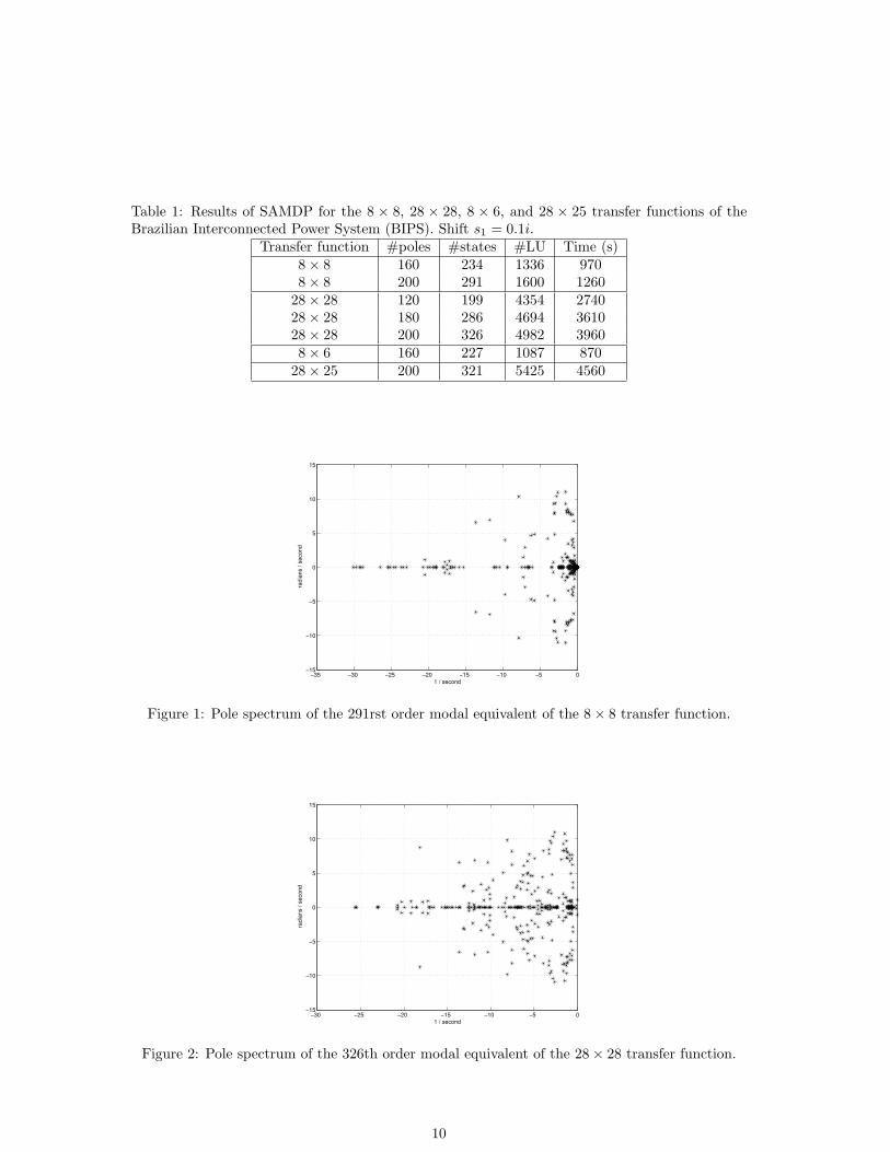
Table 1: Results of SAMDP for the 8 × 8, 28 × 28, 8 × 6, and 28 × 25 transfer functions of theBrazilian Interconnected Power System (BIPS). Shift s1 = 0.1i.

Transfer function #poles #states #LU Time (s)8× 8 160 234 1336 9708× 8 200 291 1600 1260

28× 28 120 199 4354 274028× 28 180 286 4694 361028× 28 200 326 4982 39608× 6 160 227 1087 870

28× 25 200 321 5425 4560

−35 −30 −25 −20 −15 −10 −5 0−15

−10

−5

0

5

10

15

1 / second

radi

ans

/ sec

ond

Figure 1: Pole spectrum of the 291rst order modal equivalent of the 8× 8 transfer function.

−30 −25 −20 −15 −10 −5 0−15

−10

−5

0

5

10

15

radi

ans

/ sec

ond

1 / second

Figure 2: Pole spectrum of the 326th order modal equivalent of the 28× 28 transfer function.

10

0 5 10 15−110

−100

−90

−80

−70

−60

−50

−40

−30

−20

Frequency (rad/s)

Gai

n (d

B)

Sigmaplot

Exact σmin

Exact σmax

Reduced σmin

(series) (k=234)Reduced σ

max(series) (k=234)

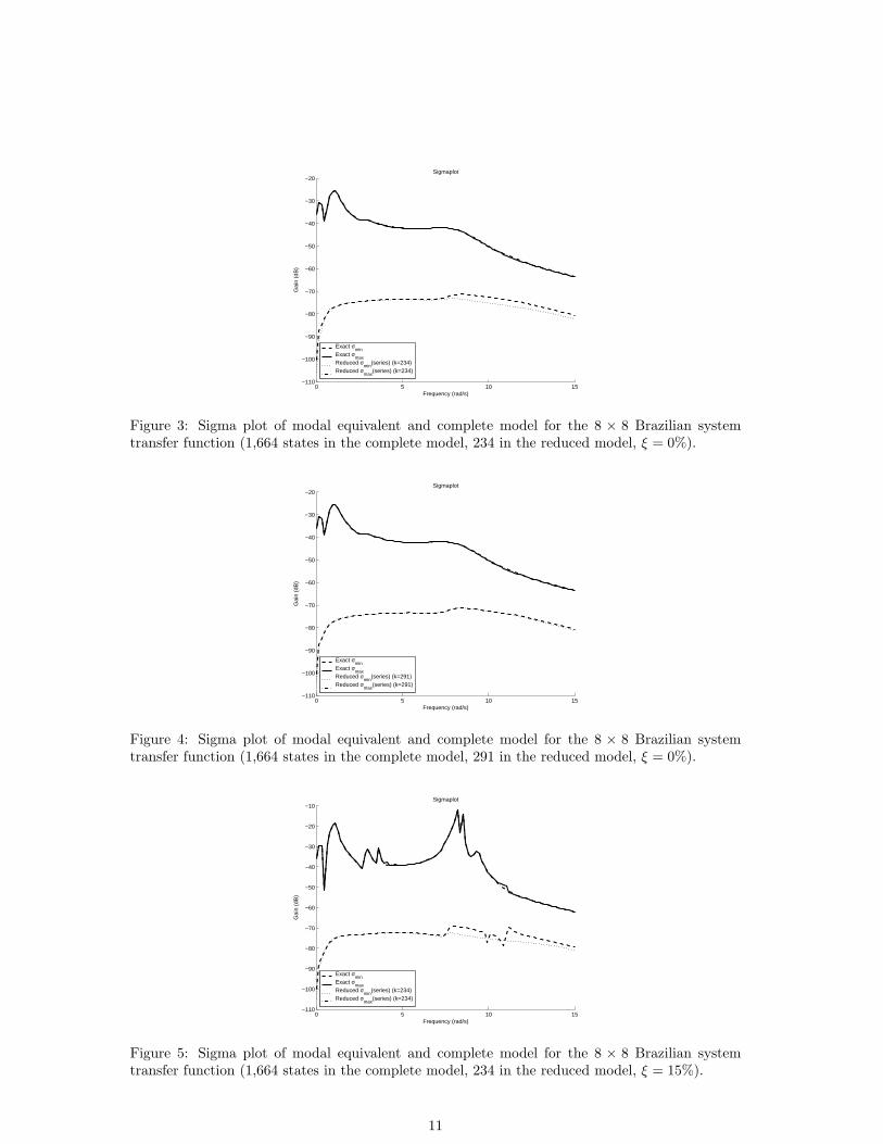
Figure 3: Sigma plot of modal equivalent and complete model for the 8 × 8 Brazilian systemtransfer function (1,664 states in the complete model, 234 in the reduced model, ξ = 0%).

0 5 10 15−110

−100

−90

−80

−70

−60

−50

−40

−30

−20

Frequency (rad/s)

Gai

n (d

B)

Sigmaplot

Exact σmin

Exact σmax

Reduced σmin

(series) (k=291)Reduced σ

max(series) (k=291)

Figure 4: Sigma plot of modal equivalent and complete model for the 8 × 8 Brazilian systemtransfer function (1,664 states in the complete model, 291 in the reduced model, ξ = 0%).

0 5 10 15−110

−100

−90

−80

−70

−60

−50

−40

−30

−20

−10

Frequency (rad/s)

Gai

n (d

B)

Sigmaplot

Exact σmin

Exact σmax

Reduced σmin

(series) (k=234)Reduced σ

max(series) (k=234)

Figure 5: Sigma plot of modal equivalent and complete model for the 8 × 8 Brazilian systemtransfer function (1,664 states in the complete model, 234 in the reduced model, ξ = 15%).

11

0 5 10 15−110

−100

−90

−80

−70

−60

−50

−40

−30

−20

−10

Frequency (rad/s)

Gai

n (d

B)

Sigmaplot

Exact σmin

Exact σmax

Reduced σmin

(series) (k=291)Reduced σ

max(series) (k=291)

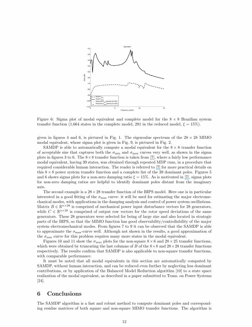
Figure 6: Sigma plot of modal equivalent and complete model for the 8 × 8 Brazilian systemtransfer function (1,664 states in the complete model, 291 in the reduced model, ξ = 15%).

given in figures 4 and 6, is pictured in Fig. 1. The eigenvalue spectrum of the 28 × 28 MIMOmodal equivalent, whose sigma plot is given in Fig. 9, is pictured in Fig. 2.

SAMDP is able to automatically compute a modal equivalent for the 8 × 8 transfer functionof acceptable size that captures both the σmin and σmax curves very well, as shown in the sigmaplots in figures 3 to 6. The 8×8 transfer function is taken from [7], where a fairly low performancemodal equivalent, having 39 states, was obtained through repeated MDP runs, in a procedure thatrequired considerable human interaction. The reader is referred to [7] for more practical details onthis 8× 8 power system transfer function and a complete list of the 39 dominant poles. Figures 5and 6 shows sigma plots for a non-zero damping ratio ξ = 15%. As is motivated in [7], sigma plotsfor non-zero damping ratios are helpful to identify dominant poles distant from the imaginaryaxis.

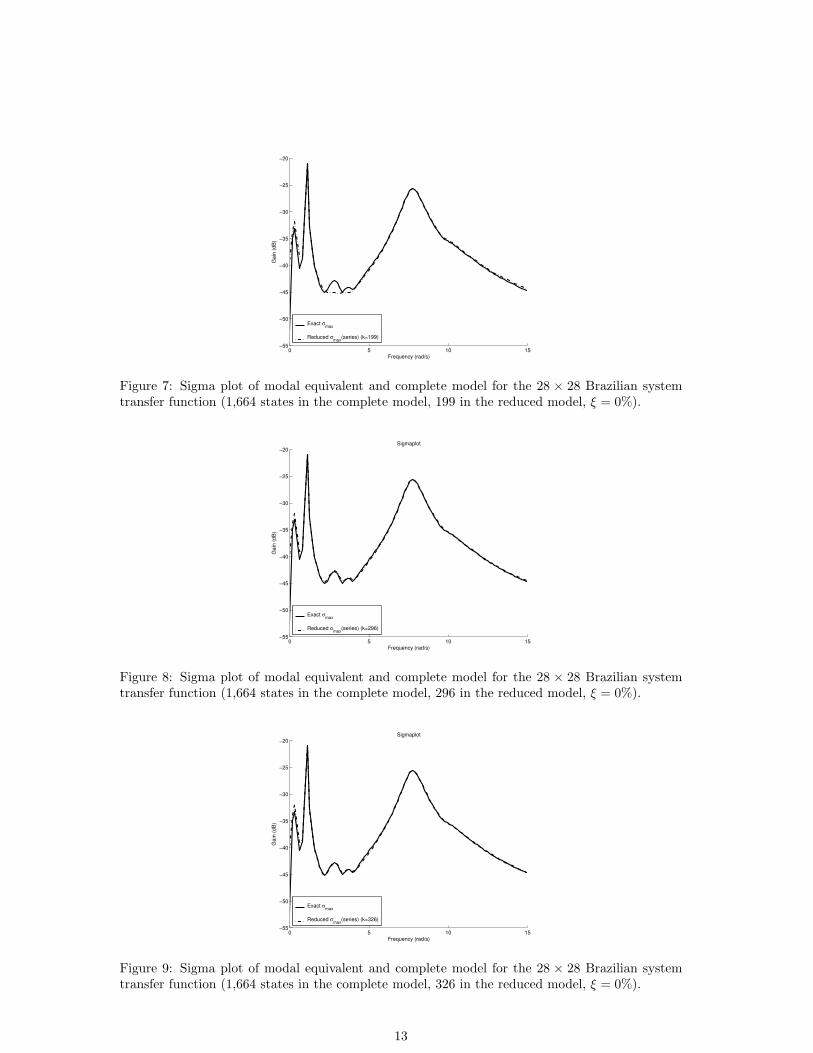
The second example is a 28×28 transfer function of the BIPS model. Here one is in particularinterested in a good fitting of the σmax curve: it will be used for estimating the major electrome-chanical modes, with applications in the damping analysis and control of power system oscillations.Matrix B ∈ Rn×28 is comprised of mechanical power input disturbance vectors for 28 generators,while C ∈ Rn×28 is comprised of output row vectors for the rotor speed deviations of the samegenerators. These 28 generators were selected for being of large size and also located in strategicparts of the BIPS, so that the MIMO function has good observability/controllability of the majorsystem electromechanical modes. From figures 7 to 9 it can be observed that the SAMDP is ableto approximate the σmax-curve well. Although not shown in the results, a good approximation ofthe σmin curve for this problem requires many more states in the modal equivalent.

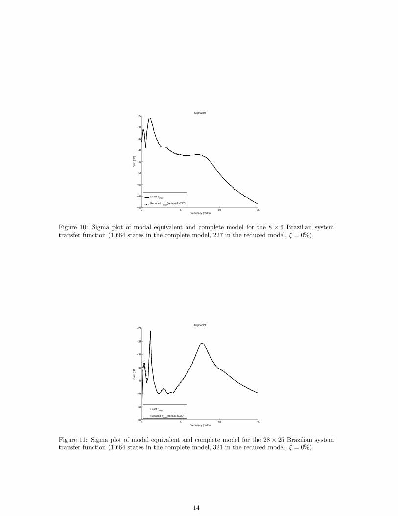
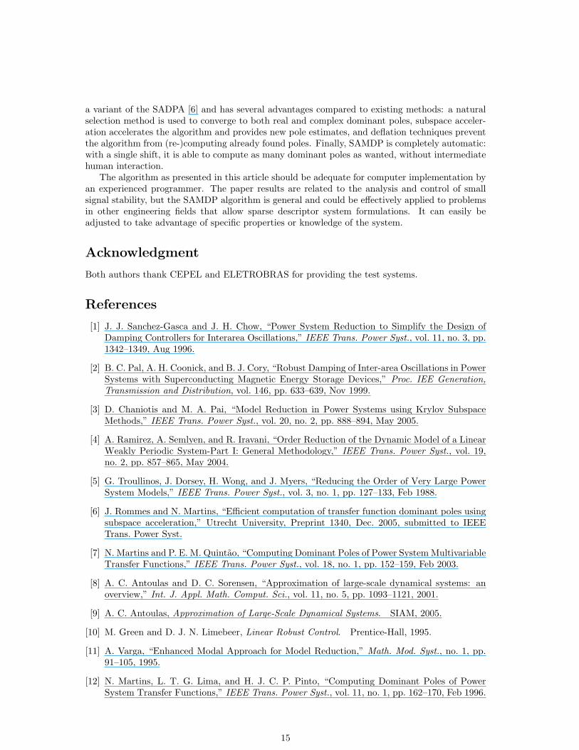
Figures 10 and 11 show the σmax plots for the non-square 8× 6 and 28× 25 transfer functions,which were obtained by truncating the last columns of B of the 8×8 and 28×28 transfer functionsrespectively. The results confirm that SAMDP is also applicable to non-square transfer functions,with comparable performance.

It must be noted that all modal equivalents in this section are automatically computed bySAMDP, without human interaction, and can be reduced even further by neglecting less dominantcontributions, or by application of the Balanced Model Reduction algorithm [10] to a state spacerealization of the modal equivalent, as described in a paper submitted to Trans. on Power Systems[24].

6 Conclusions

The SAMDP algorithm is a fast and robust method to compute dominant poles and correspond-ing residue matrices of both square and non-square MIMO transfer functions. The algorithm is

12

0 5 10 15−55

−50

−45

−40

−35

−30

−25

−20

Frequency (rad/s)

Gai

n (d

B)

Exact σ

max Reduced σ

max(series) (k=199)

Figure 7: Sigma plot of modal equivalent and complete model for the 28 × 28 Brazilian systemtransfer function (1,664 states in the complete model, 199 in the reduced model, ξ = 0%).

0 5 10 15−55

−50

−45

−40

−35

−30

−25

−20

Frequency (rad/s)

Gai

n (d

B)

Sigmaplot

Exact σ

max Reduced σ

max(series) (k=296)

Figure 8: Sigma plot of modal equivalent and complete model for the 28 × 28 Brazilian systemtransfer function (1,664 states in the complete model, 296 in the reduced model, ξ = 0%).

0 5 10 15−55

−50

−45

−40

−35

−30

−25

−20

Frequency (rad/s)

Gai

n (d

B)

Sigmaplot

Exact σ

max Reduced σ

max(series) (k=326)

Figure 9: Sigma plot of modal equivalent and complete model for the 28 × 28 Brazilian systemtransfer function (1,664 states in the complete model, 326 in the reduced model, ξ = 0%).

13

0 5 10 15−65

−60

−55

−50

−45

−40

−35

−30

−25

Frequency (rad/s)

Gai

n (d

B)

Sigmaplot

Exact σ

max Reduced σ

max(series) (k=227)

Figure 10: Sigma plot of modal equivalent and complete model for the 8 × 6 Brazilian systemtransfer function (1,664 states in the complete model, 227 in the reduced model, ξ = 0%).

0 5 10 15−55

−50

−45

−40

−35

−30

−25

−20

Frequency (rad/s)

Gai

n (d

B)

Sigmaplot

Exact σ

max Reduced σ

max(series) (k=321)

Figure 11: Sigma plot of modal equivalent and complete model for the 28 × 25 Brazilian systemtransfer function (1,664 states in the complete model, 321 in the reduced model, ξ = 0%).

14

a variant of the SADPA [6] and has several advantages compared to existing methods: a naturalselection method is used to converge to both real and complex dominant poles, subspace acceler-ation accelerates the algorithm and provides new pole estimates, and deflation techniques preventthe algorithm from (re-)computing already found poles. Finally, SAMDP is completely automatic:with a single shift, it is able to compute as many dominant poles as wanted, without intermediatehuman interaction.

The algorithm as presented in this article should be adequate for computer implementation byan experienced programmer. The paper results are related to the analysis and control of smallsignal stability, but the SAMDP algorithm is general and could be effectively applied to problemsin other engineering fields that allow sparse descriptor system formulations. It can easily beadjusted to take advantage of specific properties or knowledge of the system.

Acknowledgment

Both authors thank CEPEL and ELETROBRAS for providing the test systems.

References

[1] J. J. Sanchez-Gasca and J. H. Chow, “Power System Reduction to Simplify the Design ofDamping Controllers for Interarea Oscillations,” IEEE Trans. Power Syst., vol. 11, no. 3, pp.1342–1349, Aug 1996.

[2] B. C. Pal, A. H. Coonick, and B. J. Cory, “Robust Damping of Inter-area Oscillations in PowerSystems with Superconducting Magnetic Energy Storage Devices,” Proc. IEE Generation,Transmission and Distribution, vol. 146, pp. 633–639, Nov 1999.

[3] D. Chaniotis and M. A. Pai, “Model Reduction in Power Systems using Krylov SubspaceMethods,” IEEE Trans. Power Syst., vol. 20, no. 2, pp. 888–894, May 2005.

[4] A. Ramirez, A. Semlyen, and R. Iravani, “Order Reduction of the Dynamic Model of a LinearWeakly Periodic System-Part I: General Methodology,” IEEE Trans. Power Syst., vol. 19,no. 2, pp. 857–865, May 2004.

[5] G. Troullinos, J. Dorsey, H. Wong, and J. Myers, “Reducing the Order of Very Large PowerSystem Models,” IEEE Trans. Power Syst., vol. 3, no. 1, pp. 127–133, Feb 1988.

[6] J. Rommes and N. Martins, “Efficient computation of transfer function dominant poles usingsubspace acceleration,” Utrecht University, Preprint 1340, Dec. 2005, submitted to IEEETrans. Power Syst.

[7] N. Martins and P. E. M. Quintao, “Computing Dominant Poles of Power System MultivariableTransfer Functions,” IEEE Trans. Power Syst., vol. 18, no. 1, pp. 152–159, Feb 2003.

[8] A. C. Antoulas and D. C. Sorensen, “Approximation of large-scale dynamical systems: anoverview,” Int. J. Appl. Math. Comput. Sci., vol. 11, no. 5, pp. 1093–1121, 2001.

[9] A. C. Antoulas, Approximation of Large-Scale Dynamical Systems. SIAM, 2005.

[10] M. Green and D. J. N. Limebeer, Linear Robust Control. Prentice-Hall, 1995.

[11] A. Varga, “Enhanced Modal Approach for Model Reduction,” Math. Mod. Syst., no. 1, pp.91–105, 1995.

[12] N. Martins, L. T. G. Lima, and H. J. C. P. Pinto, “Computing Dominant Poles of PowerSystem Transfer Functions,” IEEE Trans. Power Syst., vol. 11, no. 1, pp. 162–170, Feb 1996.

15

[13] G. H. Golub and C. F. van Loan, Matrix Computations, 3rd ed. John Hopkins UniversityPress, 1996.

[14] J. M. Maciejowski, Multivariable Feedback Design. Addison-Wesley, 1989.

[15] T. Kailath, Linear Systems. Prentice-Hall, 1980.

[16] J. R. Smith, J. F. Hauer, D. J. Trudnowski, F. Fatehi, and C. S. Woods, “Transfer FunctionIdentification in Power System Application,” IEEE Trans. Power Syst., vol. 8, no. 3, pp.1282–1290, Aug 1993.

[17] R. V. Patel and N. Munro, Multivariable System Theory and Design. Pergamon, 1982.

[18] D. V. Murthy and R. T. Haftka, “Derivatives of eigenvalues and eigenvectors of a generalcomplex matrix,” Int. J. Num. Meth. Eng., vol. 26, pp. 293–311, 1988.

[19] Y. Saad, Numerical methods for large eigenvalue problems: theory and algorithms. Manch-ester University Press, 1992.

[20] B. N. Parlett, The Symmetric Eigenvalue Problem. Prentice Hall, 1980.

[21] ——, “The Rayleigh Quotient Iteration and Some Generalizations for Nonnormal Matrices,”Math. Comp., vol. 28, no. 127, pp. 679–693, July 1974.

[22] L. A. Aguirre, “Quantitative Measure of Modal Dominance for Continuous Systems,” in Proc.of the 32nd Conference on Decision and Control, December 1993, pp. 2405–2410.

[23] The Mathworks, Inc., “Matlab R13.” [Online]. Available: http://www.mathworks.com

[24] N. Martins, F. G. Silva, and P. C. Pellanda, “Utilizing Transfer Function Modal Equivalents ofLow-order for the Design of Power Oscillation Damping Controllers in Large Power Systems,”in IEEE/PES General Meeting, June 2005, pp. 2642–2648, enlarged version submitted toIEEE Trans. Power Syst.

16