Smooth local subspace projection for nonlinear noise reduction

David Chelidzea)

Department of Mechanical, Industrial & Systems Engineering, University of Rhode Island, Kingston,Rhode Island 02881, USA

(Received 30 May 2013; accepted 3 February 2014; published online 18 February 2014)

Many nonlinear or chaotic time series exhibit an innate broad spectrum, which makes noise

reduction difficult. Local projective noise reduction is one of the most effective tools. It is based on

proper orthogonal decomposition (POD) and works for both map-like and continuously sampled

time series. However, POD only looks at geometrical or topological properties of data and does not

take into account the temporal characteristics of time series. Here, we present a new smooth

projective noise reduction method. It uses smooth orthogonal decomposition (SOD) of bundles of

reconstructed short-time trajectory strands to identify smooth local subspaces. Restricting

trajectories to these subspaces imposes temporal smoothness on the filtered time series. It is shown

that SOD-based noise reduction significantly outperforms the POD-based method for continuously

sampled noisy time series. VC 2014 AIP Publishing LLC. [http://dx.doi.org/10.1063/1.4865754]

Noise reduction in nonlinear or chaotic time series is

problematic due to the inherent broad spectrum of the

deterministic component in a signal. Projective noise

reduction based on proper orthogonal decomposition has

been shown to be effective for low noise levels. Here, we

study a generalization of the local projective noise reduc-

tion method based on smooth orthogonal decomposition,

which accounts for both topological and temporal charac-

teristics of the time series. Through the analysis of syn-

thetic chaotic time series contaminated by various levels

of noise, we show that our method significantly outper-

forms the original and works even for low signal-to-noise

ratios. Thus, it provides an effective tool for noise reduc-

tion in continuously sampled chaotic time series.

I. INTRODUCTION

Many natural and engineered systems generate nonlin-

ear deterministic time series that are contaminated by ran-

dom measurement/dynamical noise. Chaotic time series have

inherently broad spectra and are not amenable to conven-

tional spectral noise filtering. Two main methods for filtering

noisy chaotic time series1–3 are (1) model based filtering4

and (2) projective noise reduction.2 While model based

reduction has some merit for systems with known analytical

models,4 projective noise reduction provides a superior alter-

native2 for experimental data. There are other methods like

adaptive filtering or the wavelet shrinkage5 method that can

work in certain cases but require an opportune selection of

parameters or some a priori knowledge of the system or the

noise mechanisms.6

In this paper, we describe a new method for nonlinear

noise reduction that is based on a smooth local subspace

identification7,8 in the reconstructed phase space.9,10 In con-

trast to identifying the tangent subspace of an attractor using

proper orthogonal decomposition (POD) of a collection of

nearest neighbor points (i.e., as in local projective noise

reduction scheme), we identify a smooth subspace that

locally embeds the attractor using smooth orthogonal decom-

position (SOD) of bundle of nearest neighbor trajectory

strands. This new method accounts for not only geometrical

information in the data but also its temporal characteristics

too. As we demonstrate later, this dramatically increases the

ability to filter low signal-to-noise-ratio (SNR) time series.

In Sec. II, ideas behind nonlinear noise reduction are dis-

cussed, followed by the description of the SOD-based algo-

rithm. Models generating test time series are introduced next,

along with the methods used in the algorithm evaluation,

which is followed by the description of results and discussion.

II. SMOOTH PROJECTIVE NOISE REDUCTION

Both POD-based local projective and SOD-based smooth

projective noise reduction methods work in the reconstructed

phase space9 of the system generating the noisy time series.

The basic idea is that at any point on the attractor, noise

leaks out into higher dimensions than the dimension of the

attractor’s tangent space at that point. Thus, by embedding

data into the higher d-dimensional space and then projecting

it down to the tangent subspace of k-dimensions reduces the

noise in the data. The differences between the methods are in

the way this tangent space is identified.

For both noise reduction methods, the noisy time series

fxigni¼1 is embedded into a d-dimensional global phase space

using delay coordinate embedding generating the vector-

valued trajectory fyign�ðd�1Þsi¼1

yi ¼ xi; xiþs; … xiþðd�1Þs½ �T ; (1)

where s is the delay time, which is usually determined using

the first minimum of the average mutual information18 for

the time series, by some other nonlinear correlation statis-

tic17 or by visual inspection.

The selection of the global embedding dimension d and

the dimension of the tangent subspace k is an important stepa)chelidze@mail.uri.edu; mcise.uri.edu/chelidze

1054-1500/2014/24(1)/013121/10/$30.00 VC 2014 AIP Publishing LLC24, 013121-1

CHAOS 24, 013121 (2014)

in both noise reduction schemes. For a noise-free time series,

a method of false nearest neighbors11,12 is usually used to

estimate the minimum necessary embedding dimension D.

However, the efficacy of this method is degraded by the

presence of noise.13 Alternatively, the embedding theorem

provides9 a measure of minimum sufficient embedding

dimension which should be greater than twice the fractaldimension14 of the attractor. The most commonly used esti-

mate of the fractal dimension is a correlation dimension,15

which is also not very robust with respect to noise. However,

for moderate noise levels, one can still get rough approxima-

tion to the correlation dimension,16 which could serve as the

upper bound on the projection dimension. In practical appli-

cations, the use of methods that are robust with respect to

noise (e.g., the minimum description length principle13 or

continuity statistic17) are more appropriate. In this paper,

however, we use synthetic time series which are artificially

contaminated with additive noise. Therefore, the size of

global embedding dimension is taken to be a slightly greater

than the minimum required embedding dimension estimated

using the clean time series and the false nearest neighbors

method.

A. Local projection subspace

In the local projective noise algorithm,19 for each point

yi in the reconstructed d-dimensional phase space, r, tempo-

rarily uncorrelated nearest neighbor points fyjig

rj¼1 are deter-

mined. The POD is applied to this cloud of nearest neighbor

points, and the optimal k-dimensional projection of the cloud

is obtained providing the needed filtered �yi (which is also

adjusted to account for the shift in the projection due to the

trajectory curvature at yi (Ref. 3)). The filtered time series

f�xigni¼1 is obtained by averaging the appropriate coordinates

in the adjusted vector-valued time series f�yign�ðd�1Þsi¼1 .

In contrast, smooth projective noise reduction works with

short strands of the reconstructed phase space trajectory.

These strands are composed of (2l þ 1) time-consecutive

reconstructed phase space points, where l is a small natural

number. Namely, each reconstructed point yk has an associ-

ated strand sk ¼ ½yk�l;…; ykþl� and an associated bundle of r

nearest neighbor strands fsjkg

rj¼1, including the original. This

bundle is formed by finding (r � 1) nearest neighbor points

fyjkg

r�1j¼1 for yk and the corresponding strands. SOD is applied

to each of these strands in the bundle and the corresponding

k-dimensional smoothest approximations to the strands

f~sjkg

rj¼1 are obtained. The filtered �yk point is determined by

the weighted average of points f~yjkg

rj¼1 in the smoothed

strands of the bundle. Finally, the filtered time series f�xigni¼1

are obtained just as in the local projective noise reduction. The

procedure can be applied repeatedly for further smoothing or

filtering. For completeness, the details of SOD and smooth

subspace approximation are given in the following sections.

B. Smooth orthogonal decomposition

The objective of POD is to obtain the best low-

dimensional approximate description of high-dimensional

data in a least squares sense.20–22 In contrast, SOD is aimed at

obtaining the smoothest low-dimensional approximations of

high-dimensional dynamical processes.7,23,24 While POD only

focuses on the spatial characteristics of the data, SOD consid-

ers both its temporal and spatial characteristics.

Consider a case where a field, y, is defined for some dstate variables fxigd

i¼1 (e.g., a system of d ordinary differen-

tial equations, d sensor measurements from some system).

Assume that this field is sampled at exactly n instants of time

(e.g., n sets of simultaneous measurements at d locations).

We arrange this data into a n� d matrix Y such that element

Yij is the sample taken at the ith time instant from the jthstate variable. We also assume that each column of Y has

zero mean (or, alternatively, we subtract the mean value

from each column). We are looking for a linear coordinate

transformation of this matrix Y

Q ¼ YW; (2)

where the columns of Q 2 Rn�d are new smooth orthogonalcoordinates (SOCs), and smooth projective modes (SPMs) are

given by the columns of W 2 Rd�d. In this transformation, Q

should contain time coordinates sorted by their roughness.

The SOD is accomplished by the following generalized

eigenvalue problem:

R wi ¼ ki_R wi; (3)

where R ¼ 1n YTY 2 Rd�d and _R ¼ 1

n_Y

T _Y 2 Rd�d are auto-

covariance matrices for d states and their time derivatives,

respectively. Eigenvalues ki are called smooth orthogonalvalues (SOVs), and wi 2 Rd are individual SPMs

ði ¼ 1;…; dÞ. The time derivative of the matrix Y is either

known analytically or can be derived numerically _Y ¼ DY,

where D is some finite difference differential operator.

Concept similar to SOD called slow feature analysis has been

also used for pattern analysis in neural science (Refs. 25–27).

C. Smooth subspace identification and dataprojection

Equation (3) can be solved using a generalized singularvalue decomposition of the matrix pair Y and _Y

Y ¼ UCUT ; _Y ¼ VSUT ; CTCþ STS ¼ I; (4)

where smooth orthogonal modes (SOMs) are given by the

columns of U 2 Rd�d, SOCs are given by the columns of

Q ¼ UC 2 Rn�d and SOVs are given by the term-by-term

division of diagðCTCÞ and diagðSTSÞ. The resulting SPMs

are the columns of the inverse of the transpose of SOMs:

W�1 ¼ UT 2 Rd�d. In this paper, we will assume that the

SOVs are arranged in descending order ðk1 � k2

� � � � � kdÞ. The magnitude of the SOVs quadratically cor-

relates with the smoothness of the SOCs.7 Please note that if

the identity matrix is substituted for _R in Eq. (3), it reduces

to the POD eigenvalue problem that can be solved by the sin-

gular value decomposition of the matrix Y.

The smoothest k-dimensional approximation to Y

(k< d) can be obtained by retaining only k columns of

013121-2 David Chelidze Chaos 24, 013121 (2014)

interest in the matrices U and U and reducing C to the corre-

sponding k� k minor. In effect, we are looking for a projec-

tion of Y onto a k-dimensional smoothest subspace. The

embedding of this k-dimensional projection into d-dimen-

sional space ð�YÞ is constructed using the corresponding

reduced matrices �U 2 Rn�k; �C 2 Rk�k, and �U 2 Rd�k as

follows:

�Y ¼ UC �UT: (5)

D. Data padding to mitigate the edge effects

SOD-based noise reduction is working on (2lþ 1)-long

trajectory strands. Therefore, for the first and last l points in

the matrix Y, we will not have full-length strands for calcula-

tions. In addition, the delay coordinate embedding procedure

reconstructs the original n-long time series into Y which has

only ½n� ðd � 1Þs�-long columns. Therefore, the first and

last ðd � 1Þs points in fxigni¼1 will not have all d components

represented in Y, while other points will have their counter-

parts in each column of Y. To deal with these truncations,

which cause unwanted edge effects in noise reduction, we

pad both ends of Y by ½lþ ðd � 1Þs�-long trajectory

segments. These trajectory segments are identified by finding

the nearest neighbor points to the starting and the end points

inside Y itself (e.g., ys and ye, respectively). Then, the corre-

sponding trajectory segments are extracted from Y: Ys

¼ ½ys�l�ðd�1Þs;…; ys�1�T

and Ye ¼ ½yeþ1;…; yeþlþðd�1Þs�T

and are used to form a padded matrix Y ¼ ½Ys; Y; Ye�. Now,

the procedure can be applied to all points in Y starting at

lþ 1 and ending at n þ l points.

III. SMOOTH NOISE REDUCTION ALGORITHM

Smooth noise reduction algorithm is schematically illus-

trated in Fig. 1. While we usually work with data in column

form, in this figure—for illustrative purpose—we arranged

arrays in row form. The particular details are explained as

follows:

(1) Delay coordinate embedding

(a) Estimate the appropriate delay time s and the mini-

mum necessary embedding dimension D for the time

series fxigni¼1.

(b) Determine the local (i.e., projection), k � D, and the

global (i.e., embedding), d � D, dimensions for

trajectory strands.

(c) Embed the time series fxigni¼1 using global embed-

ding parameters (s, d) into the reconstructed phase

space trajectory Y 2 Rðn�ðd�1ÞsÞ�d.

(d) Partition the embedded points in Y into a kd-tree for

fast searching.

(2) Padding and filtering

(a) Pad the end points of Y to have appropriate strands for

the edge points, which results in Y 2 R½nþ2lþ2ðd�1Þs��d .

(b) For each point fyignþli¼lþ1, construct a (2l þ 1)-long

trajectory strand s1i ¼ ½yi�l; …; yiþl� 2 Rð2lþ1Þ�d.

(c) For the same points yi, look up (r � 1) nearest

neighbor points that are temporarily uncorrelated

and the corresponding nearest neighbor strands

fsjig

rj¼2.

(d) Apply SOD to each of the r strands in this bundle

and obtain the corresponding k-dimensional smooth

approximations to all d-dimensional strands in the

bundle f~sjgrj¼1.

FIG. 1. Schematic illustration of smooth

projective noise reduction algorithm.

013121-3 David Chelidze Chaos 24, 013121 (2014)

(e) Approximate the base strand by taking the weighted

average of all these smoothed strands �si ¼ h~sjiij,

using weighting that diminishes contribution with

the increase in the distance from the base strand.

(3) Shifting and averaging

(a) Replace the points fyignþli¼1þl at the center of each

base strand by its approximation �yi determined

above to form �Y 2 R½nþðd�1Þs��d.

(b) Average each d smooth adjustment to each point in

the time series to estimate the filtered point

�xi ¼1

d

Xd

k¼1

�Yðk; iþ ðk � 1ÞsÞ:

(4) Repeat the first three steps until data are smoothed out or

some preset criterion is met.

IV. EVALUATING THE ALGORITHM

In this section, we evaluate the performance of the algo-

rithm by testing it on a time series generated by Lorenz

model29 and a double-well Duffing oscillator.28 The Lorenz

model used to generate chaotic time series is

_x ¼�8

3xþ yz; _y ¼�10 y� zð Þ; and _z ¼�xyþ 28y� z:

(6)

The chaotic signal used in the evaluation is obtained using

the following initial conditions (x0, y0, z0)¼ (20, 5, �5), and

the total of 60 000 points were recorded using 0.01 sampling

time period. The double-well Duffing equation used is

€x þ 0:25 _x � xþ x3 ¼ 0:3 cos t: (7)

The steady state chaotic response of this system was sampled

30 times per forcing period and a total of 60 000 points were

recorded to test the noise reduction algorithms.

In addition, a 60 000 point, normally distributed, random

signal was generated and was mixed with the chaotic signals

in 1/20, 1/10, 1/5, 2/5, and 4/5 standard deviation ratios,

which, respectively, corresponds to 5%, 10%, 20%, 40%,

and 80% noise in the signal or SNRs of 26.02, 20, 13.98,

7.96, and 1.94 dB. This results in total of five noisy time se-

ries for each of the models. The POD-based projective and

SOD-based smooth noise reduction procedures were applied

to all noise signals using total of ten iterations.

To evaluate the performance of the algorithms, we used

several metrics that include improvements in SNRs and

power spectrum, estimates of the correlation sum and short-

time trajectory divergence rates (used for estimating the

correlation dimension and short-time largest Lyapunov expo-

nent, respectively30). In addition, phase portraits were exam-

ined to gain qualitative appreciation of noise reduction

effects.

The largest Lyapunov exponent k131 characterizes the

exponential growth of the distance between two points on

the attractor that are very close initially. If this small initial

distance between points is d0 and the distance at a later

discrete time n is denoted as dn, then dn � d0 exp k1tð Þ as

d0 ! 0. Here, we used a modified algorithm by Wolf

et al.,32,33 where for a set of reconstructed points yi on their

fiducial trajectory, we look up the r temporarily uncorrelated

nearest neighbor points and track their average divergence

from the fiducial trajectory.

The correlation dimension characterizes the cumulative

distribution of distances on the attractor15,34,35 and indicates

the lower bound on the minimum number of variables

needed to uniquely describe the dynamics on the attractor.

Here, we used the modified algorithm described in Ref. 15,

where the correlation sum is estimated for the different

length scales � as

Cð�Þ ¼ 2

ðN� sÞðN� s� 1ÞXN

i¼1

XN

j¼iþsþ1

H ��kyi� yjk� �

� �D2 ;

(8)

where H is a Heavyside step function, N is the total number

of points, s is the interval needed to remove temporal corre-

lations, and D2 is the correlation dimension.

V. RESULTS

A. Lorenz model based time series

Using average mutual information estimated from the

clean Lorenz time series, a delay time of 12 sampling time

periods is determined. The false nearest neighbors algorithm

(see Fig. 2) indicates that the attractor is embedded in D¼ 4

dimensions for the noise-free time series. Even for the noisy

time series, the trends show clear qualitative change around

four or five dimensions. Therefore, six is used for global

embedding dimension (d¼ 6), and k¼ 3 is used as local pro-

jection dimension. The reconstructed phase portraits for the

clean Lorenz signal and the added random noise are shown

in Figs. 3(a) and 3(b), respectively. The corresponding power

spectral densities for the clean and the noise-added signals

are shown in Fig. 3(c). The phase portraits of POD- and

SOD-filtered signals with 5% noise are shown in Figs. 3(d)

and 3(e), respectively. Fig. 3(f) shows the corresponding

power spectral densities. In all these and the following fig-

ures, 64 nearest neighbor points are used for POD-based

FIG. 2. False nearest neighbor algorithm results for Lorenz time series.

013121-4 David Chelidze Chaos 24, 013121 (2014)

algorithm, and bundles of 9 eleven-point-long trajectory

strands are used for SOD-based algorithm. The filtered data

shown are for 10 successive applications of the noise reduc-

tion algorithms. The decrease in the noise floor after filtering

is considerably more dramatic for the SOD algorithm when

compared to the POD.

The successive improvements in SNRs after each itera-

tion of the algorithms are shown in Fig. 4, and the corre-

sponding numerical values are listed in Table I for the 5%

and 20% noise added signals. While the SNRs are

monotonically increasing for the SOD algorithm after each

successive application, they peak and then gradually

decrease for the POD algorithm. In addition, the rate of

increase is considerably larger for the SOD algorithm com-

pared to the POD, especially during the initial applications.

As seen from Table I, the SOD-based algorithm provides

about 13 dB improvement in SNRs, while POD-based algo-

rithm manages only 7–8 dB improvements.

The estimates of the correlation sum and short-time

trajectory divergence for the noise-reduced data and the

FIG. 3. Reconstructed phase portrait from Lorenz signal (a); random noise phase portrait (b); power spectrum of clean and noisy signals (c); POD-filtered

phase portrait of 5% noise added data (d); SOD-filtered phase portrait of 5% noise added data (e); and the corresponding power spectrums (f).

FIG. 4. Noisy Lorenz time series SNRs versus number of applications of POD-based (left) and SOD-based (right) nonlinear noise reduction procedures.

013121-5 David Chelidze Chaos 24, 013121 (2014)

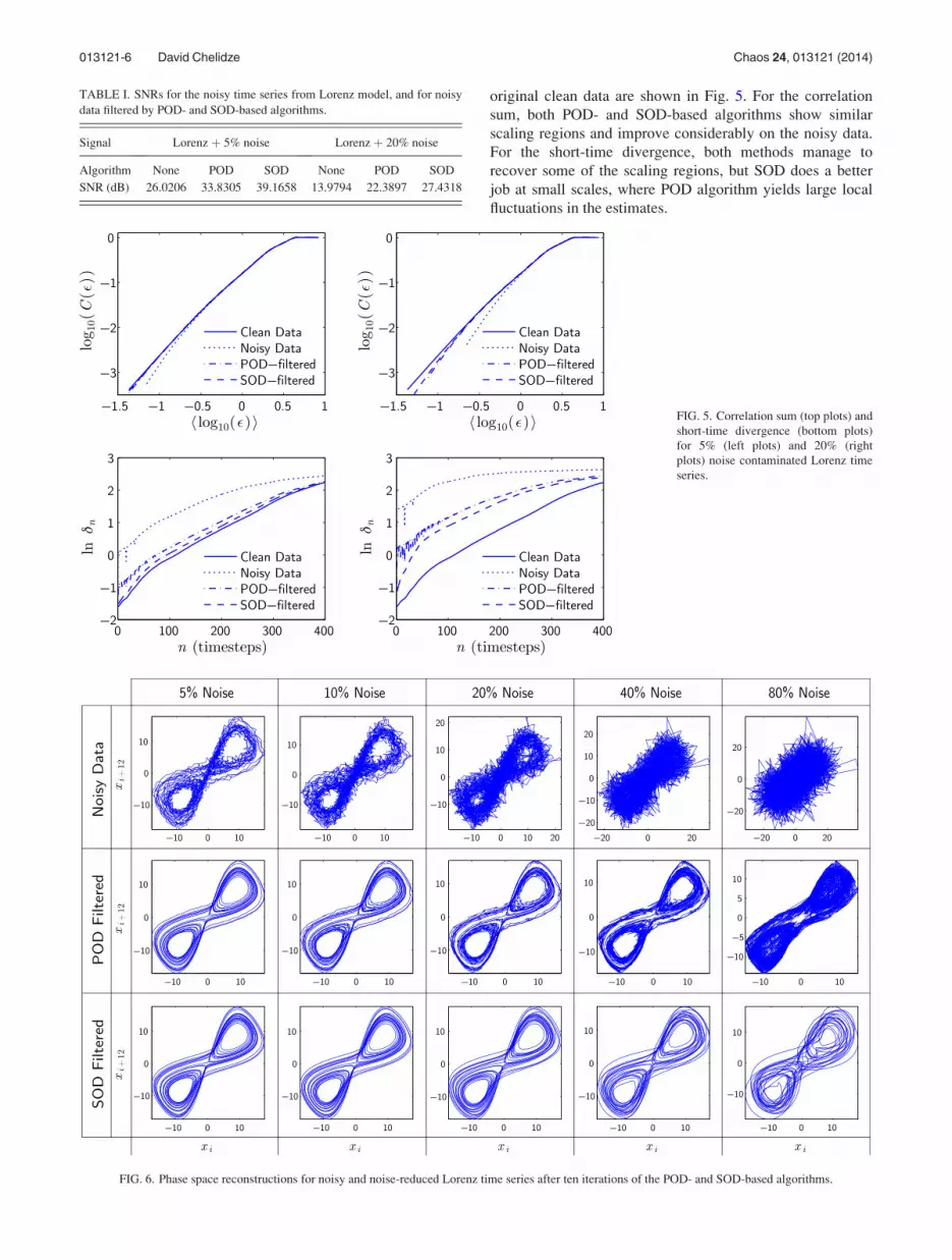
original clean data are shown in Fig. 5. For the correlation

sum, both POD- and SOD-based algorithms show similar

scaling regions and improve considerably on the noisy data.

For the short-time divergence, both methods manage to

recover some of the scaling regions, but SOD does a better

job at small scales, where POD algorithm yields large local

fluctuations in the estimates.

TABLE I. SNRs for the noisy time series from Lorenz model, and for noisy

data filtered by POD- and SOD-based algorithms.

Signal Lorenz þ 5% noise Lorenz þ 20% noise

Algorithm None POD SOD None POD SOD

SNR (dB) 26.0206 33.8305 39.1658 13.9794 22.3897 27.4318

FIG. 5. Correlation sum (top plots) and

short-time divergence (bottom plots)

for 5% (left plots) and 20% (right

plots) noise contaminated Lorenz time

series.

FIG. 6. Phase space reconstructions for noisy and noise-reduced Lorenz time series after ten iterations of the POD- and SOD-based algorithms.

013121-6 David Chelidze Chaos 24, 013121 (2014)

The qualitative comparison of the phase portraits for both

noise reduction methods are shown in Fig. 6. While POD does a

decent job al low noise levels, it fails at higher noise levels

where no deterministic structure is recovered at 80% noise level.

In contrast, SOD provides smoother and cleaner phase portraits.

Even at 80% noise level, the SOD algorithm is able to recover

large deterministic structures in the data. While SOD still misses

small scale features at 80% noise level, topological features are

still similar to the original phase portrait in Fig. 3(a).

B. Duffing equation based time series

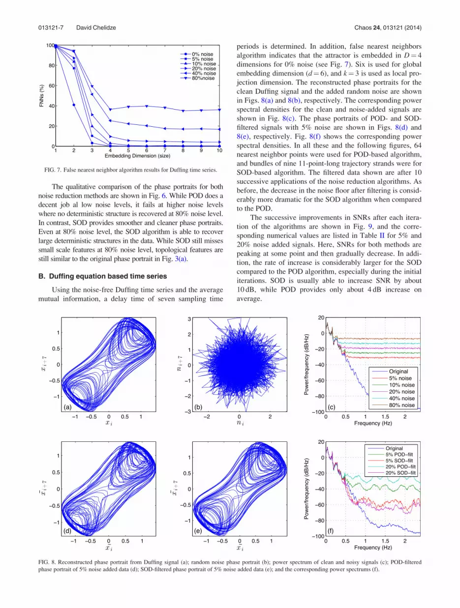
Using the noise-free Duffing time series and the average

mutual information, a delay time of seven sampling time

periods is determined. In addition, false nearest neighbors

algorithm indicates that the attractor is embedded in D¼ 4

dimensions for 0% noise (see Fig. 7). Six is used for global

embedding dimension (d¼ 6), and k¼ 3 is used as local pro-

jection dimension. The reconstructed phase portraits for the

clean Duffing signal and the added random noise are shown

in Figs. 8(a) and 8(b), respectively. The corresponding power

spectral densities for the clean and noise-added signals are

shown in Fig. 8(c). The phase portraits of POD- and SOD-

filtered signals with 5% noise are shown in Figs. 8(d) and

8(e), respectively. Fig. 8(f) shows the corresponding power

spectral densities. In all these and the following figures, 64

nearest neighbor points were used for POD-based algorithm,

and bundles of nine 11-point-long trajectory strands were for

SOD-based algorithm. The filtered data shown are after 10

successive applications of the noise reduction algorithms. As

before, the decrease in the noise floor after filtering is consid-

erably more dramatic for the SOD algorithm when compared

to the POD.

The successive improvements in SNRs after each itera-

tion of the algorithms are shown in Fig. 9, and the corre-

sponding numerical values are listed in Table II for 5% and

20% noise added signals. Here, SNRs for both methods are

peaking at some point and then gradually decrease. In addi-

tion, the rate of increase is considerably larger for the SOD

compared to the POD algorithm, especially during the initial

iterations. SOD is usually able to increase SNR by about

10 dB, while POD provides only about 4 dB increase on

average.

FIG. 7. False nearest neighbor algorithm results for Duffing time series.

FIG. 8. Reconstructed phase portrait from Duffing signal (a); random noise phase portrait (b); power spectrum of clean and noisy signals (c); POD-filtered

phase portrait of 5% noise added data (d); SOD-filtered phase portrait of 5% noise added data (e); and the corresponding power spectrums (f).

013121-7 David Chelidze Chaos 24, 013121 (2014)

The estimates of the correlation sum and short-time tra-

jectory divergence for the noisy, noise reduced data, and the

original clean data from Duffing oscillator are shown in

Fig. 10. For the correlation sum, both POD- and SOD-based

algorithms show similar scaling regions and improve sub-

stantially on the noisy data, with SOD following the noise

trend closer than POD. For the short-time divergence rates,

both methods manage to recover some of the scaling regions,

but SOD does a better job at small scales, where POD algo-

rithm causes large local fluctuations in the estimates.

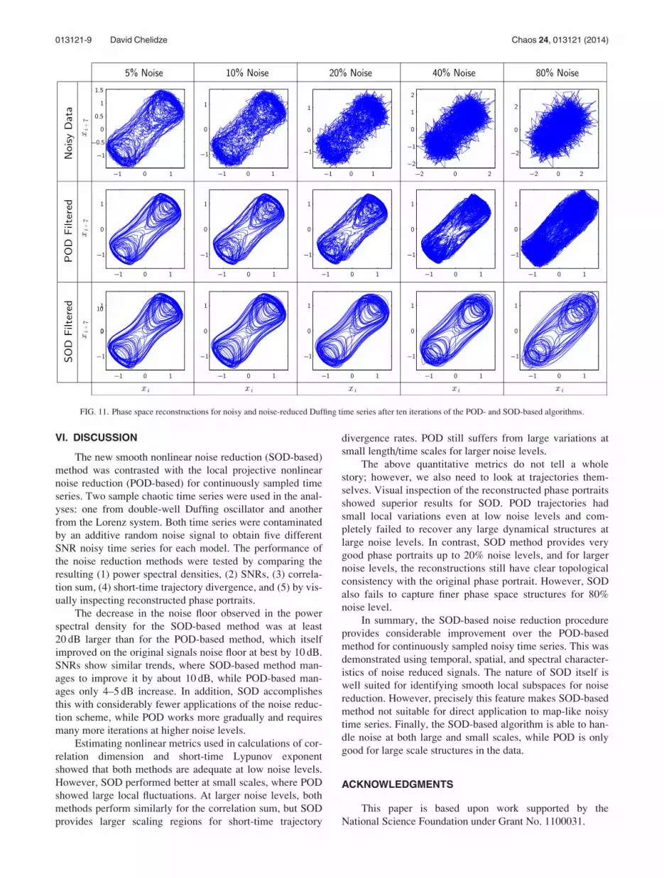
The qualitative comparison of the Duffing phase por-

traits for both noise reduction methods is shown in Fig. 11.

For consistency, all noise-reduced phase portraits are

obtained after 10 consecutive applications of the algorithms.

While POD does a decent job at low noise levels, it fails at

high noise levels where no deterministic structure is recov-

ered at 40% or 80% noise levels. In contrast, SOD provides

smoother and cleaner phase portraits at every noise level.

Even at 80% noise level, the SOD algorithm is able to

recover some large deterministic structures in the data, pro-

viding topologically similar phase portrait.

FIG. 9. Noisy Duffing time series SNRs versus number of applications of POD-based (left) and SOD-based (right) nonlinear noise reduction procedures.

TABLE II. SNRs for the noisy time series from Duffing model and for noisy

data filtered by POD- and SOD-based algorithms.

Signal Duffing þ 5% noise Duffing þ 20% noise

Filtering None POD SOD None POD SOD

SNR (dB) 26.0206 30.7583 36.1687 13.9794 19.5963 24.5692

FIG. 10. Correlation sum (top plots)

and short-time divergence (bottom

plots) for 5% (left plots) and 20% (right

plots) noise contaminated Duffing time

series.

013121-8 David Chelidze Chaos 24, 013121 (2014)

VI. DISCUSSION

The new smooth nonlinear noise reduction (SOD-based)

method was contrasted with the local projective nonlinear

noise reduction (POD-based) for continuously sampled time

series. Two sample chaotic time series were used in the anal-

yses: one from double-well Duffing oscillator and another

from the Lorenz system. Both time series were contaminated

by an additive random noise signal to obtain five different

SNR noisy time series for each model. The performance of

the noise reduction methods were tested by comparing the

resulting (1) power spectral densities, (2) SNRs, (3) correla-

tion sum, (4) short-time trajectory divergence, and (5) by vis-

ually inspecting reconstructed phase portraits.

The decrease in the noise floor observed in the power

spectral density for the SOD-based method was at least

20 dB larger than for the POD-based method, which itself

improved on the original signals noise floor at best by 10 dB.

SNRs show similar trends, where SOD-based method man-

ages to improve it by about 10 dB, while POD-based man-

ages only 4–5 dB increase. In addition, SOD accomplishes

this with considerably fewer applications of the noise reduc-

tion scheme, while POD works more gradually and requires

many more iterations at higher noise levels.

Estimating nonlinear metrics used in calculations of cor-

relation dimension and short-time Lypunov exponent

showed that both methods are adequate at low noise levels.

However, SOD performed better at small scales, where POD

showed large local fluctuations. At larger noise levels, both

methods perform similarly for the correlation sum, but SOD

provides larger scaling regions for short-time trajectory

divergence rates. POD still suffers from large variations at

small length/time scales for larger noise levels.

The above quantitative metrics do not tell a whole

story; however, we also need to look at trajectories them-

selves. Visual inspection of the reconstructed phase portraits

showed superior results for SOD. POD trajectories had

small local variations even at low noise levels and com-

pletely failed to recover any large dynamical structures at

large noise levels. In contrast, SOD method provides very

good phase portraits up to 20% noise levels, and for larger

noise levels, the reconstructions still have clear topological

consistency with the original phase portrait. However, SOD

also fails to capture finer phase space structures for 80%

noise level.

In summary, the SOD-based noise reduction procedure

provides considerable improvement over the POD-based

method for continuously sampled noisy time series. This was

demonstrated using temporal, spatial, and spectral character-

istics of noise reduced signals. The nature of SOD itself is

well suited for identifying smooth local subspaces for noise

reduction. However, precisely this feature makes SOD-based

method not suitable for direct application to map-like noisy

time series. Finally, the SOD-based algorithm is able to han-

dle noise at both large and small scales, while POD is only

good for large scale structures in the data.

ACKNOWLEDGMENTS

This paper is based upon work supported by the

National Science Foundation under Grant No. 1100031.

FIG. 11. Phase space reconstructions for noisy and noise-reduced Duffing time series after ten iterations of the POD- and SOD-based algorithms.

013121-9 David Chelidze Chaos 24, 013121 (2014)

1E. Kostelich and T. Schreiber, “Noise reduction in chaotic time-series

data: A survey of common methods,” Phys. Rev. E 48(3), 1752

(1993).2H. Kantz and T. Schreiber, Nonlinear Time Series Analysis (Cambridge

University Press, 2003), Vol. 7.3H. Kantz, T. Schreiber, I. Hoffmann, T. Buzug, G. Pfister, L. Flepp, J.

Simonet, R. Badii, and E. Brun, “Nonlinear noise reduction: A case study

on experimental data,” Phys. Rev. E 48(2), 1529 (1993).4J. Brocker, U. Parlitz, and M. Ogorzalek, “Nonlinear noise reduction,”

Proc. IEEE 90(5), 898–918 (2002).5P. Tikkanen, “Nonlinear wavelet and wavelet packet denoising of electro-

cardiogram signal,” Biol. cybern. 80(4), 259–267 (1999).6J. Gao, H. Sultan, J. Hu, and W. Tung, “Denoising nonlinear time series

by adaptive filtering and wavelet shrinkage: A comparison,” IEEE Sig.

Process. Lett. 17(3), 237–240 (2010).7D. Chelidze and W. Zhou, “Smooth orthogonal decomposition-based

vibration mode identification,” J. Sound Vib. 292(3), 461–473 (2006).8U. Farooq and B. Feeny, “Smooth orthogonal decomposition for modal

analysis of randomly excited systems,” J. Sound Vib. 316(1), 137–146

(2008).9T. Sauer, J. Yorke, and M. Casdagli, “Embedology,” J. Stat. Phys. 65(3),

579–616 (1991).10W. Liebert, K. Pawelzik, and H. Schuster, “Optimal embeddings of chaotic

attractors from topological considerations,” Europhys. Lett. 14(6), 521

(1991).11C. Rhodes and M. Morari, “False-nearest-neighbors algorithm and noise-

corrupted time series,” Phys. Rev. E 55(5), 6162–6170 (1997).12H. Abarbanel, “Local false nearest neighbors and dynamical dimen-

sions from observed chaotic data,” Phys. Rev. E 47(5), 3057–3068

(1993).13I. Ya. Molkov, D. N. Mukhin, E. M. Loskutov, and A. M. Feigin, “Using

the minimum description length principle for global reconstruction of

dynamic systems from noisy time series,” Phys. Rev. E 80(4), 046207

(2009).14J. D. Farmer, E. Ott, and J. A. Yorke, “The dimension of chaotic

attractors,” Physica D 7, 153–180 (1983).15P. Grassberger and I. Procaccia, “Measuring the strangeness of strange

attractors,” Physica D 9(1), 189–208 (1983).16R. L. Smith, “Estimating dimension in noisy chaotic time series,” J. R.

Stat. Soc., Ser. B 54(2), 329–351 (1992).17L. M. Pecora, L. Moniz, J. Nichols, and T. L. Carroll, “A unified approach

to attractor reconstruction,” Chaos 17, 013110 (2007).18A. M. Fraser and H. L. Swinney, “Independent coordinates for strange

attractors from mutual information,” Phys. Rev. A 33(2), 1134 (1986).

19N. Jevtic, J. Schweitzer, and P. Stine, “Optimizing nonlinear projective

noise reduction for the detection of planets in mean-motion resonances in

transit light curves,” Chaos 2010, 191 (2011).20A. Chatterjee, “An introduction to the proper orthogonal decomposition,”

Curr. Sci Comput. Sci. 78(7), 808–817 (2000).21M. Rathinam and L. R. Petzold, “A new look at proper orthogonal decom-

position,” SIAM J. Numer. Anal. 41(5), 1893–1925 (2003).22G. Kerschen, J.-C. Golinval, A. F. Vakakis, and L. A. Bergman, “The

method of proper orthogonal decomposition for dynamical characteriza-

tion and order reduction of mechanical systems: An overview,” Nonlinear

Dyn. 41, 147–169 (2005).23D. Chelidze and M. Liu, “Reconstructing slow-time dynamics from fast-time

measurements,” Philos. Trans. R. Soc. London A 366, 729–3087 (2008).24A. Chatterjee, J. P. Cusumano, and D. Chelidze, “Optimal tracking of pa-

rameter drift in a chaotic system: Experiment and theory,” J. Sound Vib.

250(5), 877–901 (2002).25L. Wiskott and P. Berkes, “Is slowness a learning principle of the visual

cortex?,” in Proc. Jahrestagung der Deutschen Zoologischen Gesellschaft2003, Berlin, 9–13 June, 2003 [special issue of Zoology 106(4), 373–382

(2003)].26L. Wiskott, “Unsupervised learning of invariances in a simple model of

the visual system,” in Proceedings of the 9th Annual ComputationalNeuroscience Meeting, CNS 2000, Brugge, Belgium, 16–20 July (Bochum

Research Bibliography, 2000), p. 157.27L. Wiskott, “Learning invariance manifolds,” in Proceedings of the

Computational Neuroscience Meeting, CNS’98, Santa Barbara, 1999 [spe-

cial issue of Neurocomputing 26/27, 925–932 (1999)].28I. Kovacic and M. J. Brennan, The Duffing Equation: Nonlinear

Oscillators and Their Behaviour (Wiley, 2011).29I. Stewart, “Mathematics: The Lorenz attractor exists,” Nature 406(6799),

948–949 (2000).30T. Ivancevic, L. Jain, J. Pattison, and A. Hariz, “Nonlinear dynamics and

chaos methods in neurodynamics and complex data analysis,” Nonlinear

Dyn. 56(1–2), 23–44 (2009).31J. B. Dingwell, “Lyapunov exponents,” in Wiley Encyclopedia of

Biomedical Engineering (Wiley, 2006).32A. Wolf, J. Swift, H. Swinney, and J. Vastano, “Determining lyapunov

exponents from a time series,” Physica D 16(3), 285–317 (1985).33A. Wolf, “Quantifying chaos with lyapunov exponents,” in Chaos

(Manchester University Press, 1986), pp. 273–290.34P. Grassberger and I. Procaccia, “Characterization of strange attractors,”

Phys. Rev. Lett. 50(5), 346–349 (1983).35P. Grassberger, “Generalized dimensions of strange attractors,” Phys. Lett.

A 97(6), 227–230 (1983).

013121-10 David Chelidze Chaos 24, 013121 (2014)