Efficient synthesis of tension modulation in strings and membranes based on energy estimation

Efficient synthesis of tension modulation in strings andmembranes based on energy estimation

Federico Avanzinia) and Riccardo MarognaDepartment of Information Engineering, University of Padova, Via G. Gradenigo 6/A, IT-35131, Padova, Italy

Balazs BankDepartment of Measurement and Information Systems, Budapest University of Technology and Economics,Budapest, Hungary

(Received 29 November 2010; revised 4 March 2011; accepted 6 March 2011)

String and membrane vibrations cannot be considered as linear above a certain amplitude due to the

variation in string or membrane tension. A relevant special case is when the tension is spatially con-

stant and varies in time only in dependence of the overall string length or membrane surface. The

most apparent perceptual effect of this tension modulation phenomenon is the exponential decay of

pitch in time. Pitch glides due to tension modulation are an important timbral characteristic of

several musical instruments, including the electric guitar and tom-tom drum, and many ethnic

instruments. This paper presents a unified formulation to the tension modulation problem for one-

dimensional (1-D) (string) and two-dimensional (2-D) (membrane) cases. In addition, it shows that

the short-time average of the tension variation, which is responsible for pitch glides, is approxi-

mately proportional to the system energy. This proportionality allows the efficient physics-based

sound synthesis of pitch glides. The proposed models require only slightly more computational

resources than linear models as opposed to earlier tension-modulated models of higher complexity.VC 2012 Acoustical Society of America. [DOI: 10.1121/1.3651097]

PACS number(s): 43.75.Hi, 43.75.Mn, [NHF] Pages: 897–906

I. INTRODUCTION

The main features of string and membrane oscillation

are well described by the one- and two-dimensional (1- and

2-D, respectively) linear wave equation. However, some rel-

evant secondary effects can only be accounted for by aban-

doning the hypothesis of linear vibration. In particular, the

assumption of constant tension does not hold above a certain

vibration amplitude because the tension depends on the dis-

placement. This type of nonlinearity is termed “geometric

nonlinearity” because it comes from the geometry of the

problem (the elasticity of the material is assumed to be

linear).

The effects of the geometric nonlinearity in strings are

classified into different regimes, depending on the parame-

ters of the string and excitation force.1 These are listed in

Table I, showing the significance of transverse to longitudi-

nal coupling (T!L), longitudinal to transverse coupling

(L!T), and longitudinal inertial effects. Various models

have been proposed1–3 to accurately simulate these regimes.

However, they are computationally demanding, and their ac-

curacy is not always required because, depending on the

instrument considered, only a subset of nonlinear phenom-

ena are perceptually relevant.

The tension modulation regime is found when the ten-

sion varies in time but it is spatially uniform along the string.

This happens when the bandwidth of the nonlinear excitation

force from the transverse vibration is below the longitudinal

modal frequencies, so that the inertial effects of the longitu-

dinal motion are negligible and longitudinal motion immedi-

ately follows transverse motion to find an equilibrium in the

force, resulting in uniform tension. Tension modulation is

particularly relevant for certain instruments (e.g., electric

and steel-stringed acoustic guitars and various ethnic instru-

ments4), its most perceptually prominent effect being the

decrease in pitch as the sound decays. In other cases, other

phenomena may be relevant. As an example, for the piano,

string longitudinal inertial effects come into play, while lon-

gitudinal to transverse coupling can be neglected.1

For the membrane, there appears to be no previous study

about regimes of oscillations due to the geometric nonlinear-

ity. However, pitch glides due to tension modulation are

known to be perceptually also very significant in mem-

branes. An example is the tom-tom drum, where characteris-

tic glides can be heard at medium-high dynamic ranges.5

Therefore, there is a strong motivation to simulate tension

modulation in physics-based synthesis.

The nonlinear motion of a tension-modulated string was

already investigated by Kirchhoff, then revisited by Carrier.6

All later tension modulated models proposed in the fields of

musical acoustics and sound synthesis are based on the

Kirchhoff–Carrier approach.

In the context of physically based sound synthesis, the

first study on tension modulation is by Karjalainen et al.,7

who developed a nonlinear string model for the kantele (a

Finnish traditional instrument), using digital waveguides.8

Since then, various approaches have been presented in the

framework of waveguide modeling: In general, the effect of

tension variation can be simulated by varying the delay line

a)Author to whom correspondence should be addressed. Electronic mail:

[email protected]

J. Acoust. Soc. Am. 131 (1), Pt. 2, January 2012 VC 2012 Acoustical Society of America 8970001-4966/2012/131(1)/897/10/$30.00

Au

tho

r's

com

plim

enta

ry c

op

y

length, which can be achieved through a variable allpass fil-

ter at the termination.4,9 The string tension is estimated at

each time instant, then the instantaneous propagation speed

and the required length change in the delay line are obtained.

The calculation of the tension is demanding and increases

the computational load significantly compared with linear

string models. The computational complexity is further

increased if the variable length delays are distributed

between the delay elements for better accuracy.10,11

String models based on modal synthesis12 are also

widely used. In this context, a tension-modulated string

model has been proposed by Rabenstein and Trautmann13

that is based on the so-called functional transformation

method (FTM)14 to derive modal parameters. Bilbao also

proposed a modal-type approach,15 which, unlike other

modal synthesis realizations, has an energy-conservation

property by which the stability of the numerical model is

guaranteed by construction. In finite-difference models, it is

relatively straightforward to simulate tension modulation by

changing the tension parameter of a linear string model. An

energy-conserving scheme was presented by Bilbao.16

Compared with strings, tension modulation in mem-

branes is discussed in a significantly smaller amount of liter-

ature. Early linear membrane models were mainly based on

digital waveguide meshes,17 which can provide accurate

simulation of wave propagation, depending on mesh topol-

ogy18 and methods to compensate for dispersion.19 However,

nonlinear models accounting for tension modulation were

developed mostly in the context of modal synthesis. Raben-

stein and coworkers proposed an extension of their FTM

approach to the 2-D case of tension-modulated rectangular

membranes.20

More general theories for large amplitude vibrations of

membranes are typically derived from theories for thin plates

subjected to lateral and in-plane forces.21,22 One of the most

widely used theories was developed by von Karman.23 In

this approach, plate vibrations are modeled by two nonli-

nearly coupled PDEs, one for transverse displacement and

one for a stress function. The von Karman equations have

been applied to the sound synthesis of plates.24,25 More

recently, a tension-modulated circular membrane model was

proposed26,27 based on the so-called Berger approximation

of the von Karman equations.23,28 A finite-difference

tension-modulated membrane model has also been recently

proposed.29

Even for the simplest models of tension modulation in

strings and membranes, the computational complexity is sig-

nificantly higher than for efficient linear models. This paper

presents a novel approach, which leads to a simplified

description and to significant computational savings in nu-

merical simulations, while still allowing simulation of the

perceptually most relevant effect of tension modulation. It is

shown that the so-called “quasistatic” component (i.e., the

short-time average) of the nonlinear tension, which is re-

sponsible for the pitch glide effect, can be estimated from

the total energy of the system. Moreover, the system energy

can be computed at significantly lower computational costs

than the tension. As such, the proposed approach is particu-

larly relevant for applications in the context of physically

based sound synthesis of musical instruments and makes it

possible to include tension modulation in string and

membrane synthesis in less powerful computational

environments.

Preliminary results have been already presented for the

the string30 and the circular membrane.31 This paper extends

these results in several respects. First, a general formulation

is proposed that specializes to the 1-D case of the string and

to the 2-D case of the membrane with circular and rectangu-

lar geometries. While the methodology can be used for sev-

eral types of excitation, here it is demonstrated for the case

of hammer impact. For this case, a further simplified

approach to energy computation is presented that computes

the quasistatic component of tension with a negligible com-

putational overhead compared with linear models. The

results are demonstrated by numerical simulations of string

and membrane vibrations, using both modal synthesis (for

the membranes) and finite-difference approaches (for the

string).

The remainder of the paper is organized as follows. Sec-

tion II describes the general initial and boundary value prob-

lem and shows that it includes the Kirchhoff–Carrier

equation and the Berger equations as special cases. The

modal solution is presented in Sec. III, which also shows

that the spatially uniform tension can be written in terms of

the normal modes. Section IV illustrates the main ideas of

the proposed approach and relates the total energy of the

system to the tension. Finally, Sec. V applies these results to

the efficient synthesis of tension-modulated strings and

membranes.

II. SPATIALLY UNIFORM TENSION MODULATION INSTRINGS AND MEMBRANES

A. General formulation

Throughout the paper, the following equation of

motion is considered for the displacement z(x, t) defined

over the d–dimensional domain S � Rd d ¼ 1; 2ð Þ:

Dr4zþ q@2z

@t2� TðzÞr2zþ d1

@z

@t� d3

@r2z

@t¼ f ðextÞ; (1)

where spatial and temporal dependencies (x, t) (with x 2 Sand t 2 R) have been omitted for brevity. The term

f extð Þ x; tð Þ on the right-hand side is an external force density

(in N/md) acting on the system. The operators r2 and

r4 ¼ r2 � r2 are the d-dimensional Laplacian and bihar-

monic operator, respectively. The constant q is the material

density (in kg/md), while the function T(z) represents tension

TABLE I. Main features of the different regimes of string behavior.

The� sign means that the specific feature of vibration is significant.

Regime T! L L! T L inertial eff.

Linear motion

Double freq. terms �Tension modulation � �Longotudinal modes � �Bidirectional coupling � � �

898 J. Acoust. Soc. Am., Vol. 131, No. 1, Pt. 2, January 2012 Avanzini et al.: Energy based tension modulation synthesis

Au

tho

r's

com

plim

enta

ry c

op

y

(in N/md–1). We model all types of losses (internal and air

losses, losses at the boundary) by the terms with first-order

time derivatives and by the d1, d3 coefficients. The fourth-

order term accounts for the effect of the bending stiffness D,which is proportional to the Young’s modulus of the material

(the constant of proportionality depends on the dimensional-

ity and geometry of the problem). Bending stiffness is

assumed to be small D=T � 1ð Þ throughout the paper.

Note that Eq. (1) considers the case of spatially uniform

tension, i.e., T does not depend on the point x, but is a func-

tion of the overall displacement function z only. The func-

tion T(z) is assumed to have the following form:

TðzÞ ¼ T0 þ TNLðzÞ; (2)

where T0 is the tension at rest, while TNL depends nonli-

nearly on the displacement. The following form is consid-

ered for TNL:

TNLðzÞ ¼ CNLSðzÞ � S0

S0

’ 1

2

CNL

S0

ðSjjrzjj2dx; (3)

where S(z) represents the “extension” (e.g., the string length

or the membrane area) spanned by the displacement z over

the set S, and S0 ¼ S zð Þjz¼0 is the extension at rest. The gen-

eral assumption behind Eq. (3) is that tension modulation

only depends on the total variation of the extension S(z). The

integral in Eq. (3) approximates the variation of S(z). The

symbol r indicates gradient, while the constant CNL depends

on the problem dimensionality and geometry. The meaning

of Eq. (3) is further clarified through the special cases dis-

cussed next.

B. Special cases

The preceding general formulation includes two rele-

vant special cases: the Kirchhoff–Carrier equation6 for the

tension-modulated string, and the Berger equations for the

tension-modulated membrane.23

Equation (1) with d¼ 1 describes the displacement z(x, t)of a string, where S ¼ x : x 2 0; L0½ �f g and L0 is the string

length at rest. In this case, q (in kg/m) is the string linear

density and D¼Qaj2 is the bending stiffness (with Q, Young

modulus; a, cross-sectional string area; j, radius of gyration).

According to the Kirchhoff–Carrier equation, spatially uni-

form tension of the string at large displacements is approxi-

mated by

TNLðzÞ ’1

2

Qa

L0

ðL0

0

dz

dx

� �2

dx: (4)

The integral represents the increase of string length at large

displacements, L(z), with respect to the length at rest L0.

This is a special case of Eq. (3) with CNL¼Qa, and with the

string length L(z) having the role of the extension S(z) in the

general formulation:

TNLðzÞ ¼ QaLðzÞ � L0

L0

: (5)

Equation (1) with d¼ 2 describes the displacement z(x, t) of

a membrane. For a rectangular membrane, S ¼ x ¼ x; yð Þ :fx 2 0; Lx½ �; y 2 0; Ly

� �g;where Lx and Ly are the membrane

lengths at rest in the x and y directions, respectively. For a cir-

cular membrane, S¼ x¼ r;uð Þ : r2 0;R½ �;u2 0;2pÞ½f g;where

R is the membrane radius. In both cases, q (in kg/m2) is the

membrane surface density and D¼Qh3=12 1��2ð Þ is the

bending stiffness (where Q is the Young modulus, h is

the membrane height, and � is the Poisson ratio).

A model of spatially uniform tension in a membrane at

large displacement is provided by the Berger approximation

of von Karman theory.23,28 For the rectangular membrane,

the Berger approximation can be restated as:

TNLðzÞ ’Qh

2LxLyð1� �2Þ

�ðLx

0

ðLy

0

@z

@x

� �2

þ @z

@y

� �2" #

dxdy:

(6)

For the circular membrane, the equation becomes:

TNLðzÞ ’Qh

2pR2 1� t2ð Þ

�ðR

0

ð2p

0

@z

@r

� �2

þ 1

r2

@z

@u

� �2" #

rdudr:

(7)

These equations can be interpreted as the 2-D version of Eq.

(4) because the double integrals represent the increase in

membrane area at large displacements, A(z), with respect to

the area at rest A0.26 Thus Eqs. (6) and (7) are special cases

of Eq. (3) with CNL ¼ Qh= 1� t2ð Þ; and with the membrane

area A(z) having the role of the extension S(z) in the general

formulation:

TNLðzÞ ¼Qh

1� t2

AðzÞ � A0

A0

; (8)

independently of the membrane geometry.

Figure 1 exemplifies the effects of spatially uniform ten-

sion modulation in two cases. Figure 1(a) shows a synthetic

example of a rigidly terminated, tension-modulated string,

obtained from a finite-difference model. The pluck exciting

the string is modeled as a triangle-shaped initial displace-

ment distribution with a peak value of 5 mm. The finite-

difference model is a variation of the linear model of

Chaigne and Askenfelt,32 in which the tension parameter

varies according to the tension computed from the string dis-

placement by the discretized version of Eq. (4). Figure 1(b)

shows a synthetic example of a tension-modulated circular

membrane, obtained using modal synthesis and an impact

force model that simulates interaction with a hammer or

mallet26 with impact velocity 10 m/s, that is well below the

highest dynamic levels in drum playing.33

For the string example, the tension at rest is T0¼ 100 N,

whereas for the membrane, it is T0¼ 1 500 N/m. Therefore

in both cases, the magnitude of TNL is a significant fraction

of T0 and causes audible pitch glides. In the same figures, the

dashed lines show the short-time average (quasistatic)

J. Acoust. Soc. Am., Vol. 131, No. 1, Pt. 2, January 2012 Avanzini et al.: Energy based tension modulation synthesis 899

Au

tho

r's

com

plim

enta

ry c

op

y

tension variation. The slow initial rise of this tension compo-

nent occurs because this has been estimated by applying a

running average filter to TNL.

III. MODAL SOLUTION

A. General formulation

Equation (1) has a unique solution for given boundary

and initial conditions. Here we consider the case of zero dis-

placement and zero second-order spatial derivative on the

boundary. The latter condition is needed if the fourth-order

term is considered in Eq. (1).

Let us first consider Eq. (1) in the linear case

TNL zð Þ � 0ð Þ: Recall that a mode is a particular solution in

which temporal and spatial dependencies are decoupled.

With the considered boundary conditions, Eq. (1) has a

numerable set of modes

�zgðtÞKgðxÞ; g 2Nd; (9)

where d is the dimension of the problem. In the hypothesis

of vanishingly small bending stiffness and dissipation, the

space-dependent functions Kg (i.e., the modal shapes) are the

eigenfunctions of the operator r2 satisfying the boundary

conditions of the problem:

r2KgðxÞ ¼ �kgKgðxÞ; (10)

where – kg (with kg> 0) are the corresponding eigenvalues.

Therefore the functions Kg depend on the dimensionality and

on the geometry of the problem.

The modal solution is associated with a Sturm–Liouville

(SL) transform, an integral operator whose kernel is given

by the spatial eigenfunctions.14 The SL transform �z of z and

the inverse SL transform are defined as

�zgðtÞ ¼ðS

zðx; tÞKgðxÞdx; (11a)

zðx; tÞ ¼X

g

�zgðtÞKgðxÞjjKgðxÞjj22

; (11b)

where ||�||2 is the norm in L2 (S). Equation (11b) expresses

the displacement z(x, t) as the series of its normal modes,

with shapes Kg(x) and amplitudes �zg tð Þ:By substituting Eq. (11b) into the linear equation of

motion Eq. (1) and applying Eq. (11a), one obtains a set of

second-order ordinary differential equations that describe the

dynamics of the normal modes:

€�zg þd1 þ d3kg

q_�zg þ kg kg

D

qþ c2

� ��zg ¼

�fðextÞg

q; (12)

where

�f ðextÞg ¼

ðS

f ðextÞðx; tÞKgðxÞdx (13)

is the excitation force acting on mode g; and c ¼ffiffiffiffiffiffiffiffiffiffiT0=q

pis

the propagation speed. The solutions for the homogenous

part �fextð Þ

g ¼ 0� �

of Eq. (12) are exponentially decaying

sinusoids:

�zgðtÞ ¼ Ag sinðxgtþ /gÞe�t=sg; (14)

where amplitudes Ag and phases /g depend on the initial

conditions. The modal frequencies xg and decay times sg

depend on the parameters in Eq. (12):

x2g ¼ kg

D

qkg þ c2

� � kgc2; (15a)

s�1g ¼

1

2qðd1 þ d3kgÞ; (15b)

where Eq. (15a) holds because D=T0 ¼ D= qc2ð Þ � 1:Let us now take into account the nonlinear tension. The

term involving TNL can be moved to the right-hand side of

Eq. (1) and regarded as an additional force f tmð Þ zð Þ ¼TNL zð Þr2z acting on the system. Applying the SL transform

to f (tm) yields, for the gth mode:

FIG. 1. Simulated nonlinear tension TNL (solid) and quasistatic tension com-

ponent (dashed) in two cases: (a) electric guitar string with L0¼ 65 cm,

plucked at point 0.12L0; (b) circular membrane with R¼ 16 cm, hit with ve-

locity 10 m/s at point 0.5R.


Au

tho

r's

com

plim

enta

ry c

op

y

�f ðtmÞg ð�z; zÞ ¼ðS

TNLðzÞr2z� �

Kgdx ¼ �kgTNLðzÞ�zg: (16)

This tension modulation force can be incorporated into Eq.

(12) in a similar way to �fextð Þ

g : By substituting Eq. (11b) into

Eq. (3), and exploiting mode orthogonality, TNL in Eq. (3) is

written as a function of the modes:

�TNLð�zÞ ¼1

2

CNL

S0

Xg

kg�z2gðtÞ

jjKgjj22: (17)

Therefore �ftmð Þ

g can be written as

�f ðtmÞg ð�zÞ ¼ �kg1

2

CNL

S0

X�g

k�g�z2gðtÞ

jjK�gjj22

" #�zg: (18)

B. Special cases

Again the preceding general formulation can be specialized

to the relevant cases under examination, i.e., the tension

modulated string and membrane with fixed boundary condi-

tions. Modal solutions for these systems are known and are

summarized next.

For the string, spatial eigenfunctions are:34

KnðxÞ ¼ sinnpx

L0

� �; (19)

where n ¼ 0; :::;þ1: These satisfy

r2KnðxÞ ¼ �knKnðxÞ;with kn ¼npL0

� �2

: (20)

For the rectangular membrane, the spatial eigenfunctions

are:35

Kn;mðx; yÞ ¼ sinnpx

Lx

� �sin

mpy

Ly

� �; (21)

where n;m ¼ 0; :::;þ1: These satisfy

r2Kn;mðx; yÞ ¼ �kn;mKn;mðx; yÞ;

with kn;m ¼ p2 n

Lx

� �2

þ m

Ly

� �2" #

:(22)

For the circular membrane, the spatial eigenfunctions are35:

Kn;mðr;uÞ ¼ cosðnuÞJn

�ln;m

r

R

�; (23)

where n ¼ 0; :::;þ1;m ¼ 1; :::;þ1;and ln;m is the mth

zero of the nth order Bessel function of the first kind, Jn.These satisfy

r2Kn;mðxÞ ¼ �kn;mKn;mðxÞ;with kn;m ¼ln;m

R

� �2

: (24)

Equations (19), (21), and (23) are all special cases of the

general modal solution, with g¼ n for the string and

g ¼ n;mð Þ for the membrane.

IV. ENERGY-BASED MODEL OF TENSIONMODULATION

Because the most prominent perceptual effect of tension

modulation in strings and membranes is the pitch glide due

to the quasistatic variation of the tension with oscillation am-

plitude, it is reasonable to focus on the modeling of this

effect only. In this section, we first show that the quasistatic

tension component is responsible for the pitch glide effect

and then derive a simple relationship between this compo-

nent and the energy of the system. As will be shown later,

the energy of the system can be estimated at lower computa-

tional complexity, thus allowing computation of the quasi-

static tension with less operations than earlier tension

modulation models.

A. Quasistatic tension modulation

The nonlinear tension can be split into a quasistatic

component and a second one containing double-frequency

terms. By substituting Eq. (14) into Eq. (17), one finds:

�TNLð�zÞ¼CNL

2S0

Xg

kgA2g

jjKgjj221�cosð2xgtþ2/gÞ� �

e�2t=sg :(25)

The first time-dependent part of Eq. (25) is a quasistatic vari-

ation of tension:

TqsðtÞ ¼1

2

CNL

S0

Xg

kgA2g

jjKgjj22� e�2t=sg ; (26)

which decays slowly with respect to the oscillation periods

2p=xg: This leads to a shift (continuous decrease) in the

modal frequencies, resulting in a pitch glide. Figures 1(a)

and 1(b) show estimates of Tqs tð Þ for the plucked string and

the struck membrane obtained by applying a lowpass filter to

the respective TNL signals.

The second part of Eq. (25) contains the double fre-

quency terms

Tdf ðtÞ ¼ �CNL

2S0

Xg

kgA2g

jjKgjj22cosð2xgtþ 2/gÞe�2t=sg (27)

and produces a continuous modulation of tension, built up

by sinusoidal functions with doubled oscillation frequencies

compared with the corresponding modal frequencies. The

amplitude of this modulation decays exponentially, and the

decay times of its components are halved with respect to

the modal ones.

For the string, the effect of the double frequency terms

has been discussed in the literature.36 If the string is rigidly

terminated, transverse modes cannot efficiently exchange

energy and double frequency terms do not have an effect in

practice, and only the quasi-static part is relevant. If the

bridge is not infinitely rigid (so that the modal shapes are not

anymore orthogonal), all the modes can gain energy from

the bridge motion. However, this mode coupling effect is not

significant for most western string instruments due to the


Au

tho

r's

com

plim

enta

ry c

op

y

large difference in the order of magnitude of string and

bridge admittances.

For the membrane, the effect of double frequency terms

has not been discussed in the literature to our knowledge and

is an interesting topic for future research. We assume that

the various modes might gain energy from each other even

for rigid terminations due to the much higher modal density

than that of the string. Nevertheless, modeling only the qua-

sistatic part still captures the most relevant perceptual fea-

tures of tension modulation as will be demonstrated by the

examples in Sec. V.

B. Energy

The following derivations can be found in acoustics

textbooks37 and are summarized here to make the paper

self-explanatory. The kinetic energy of an element dx is

dEk(x, t)¼ 1=2qdx _z2 x; tð Þ: The total kinetic energy is

EkðtÞ ¼q2

ðS

@zðx; tÞ@t

2

dx: (28)

The potential energy Ep can be derived as follows. Consider

a path that goes from equilibrium to the final displacement z,through the intermediate displacements kz with k 2 0; 1½ �ð Þ:The potential energy equals the work done by the system

forces along this path. Throughout the path, the force acting

on an element dx is

Fðx; kÞ ¼ T0r2kzðx; tÞdx: (29)

At the final displacement z, the potential energy dEp of the

element dx equals (with opposite sign) the work done by this

force along the whole path. For each increase dk, the corre-

sponding change in displacement is zdk, thus:

dEpðx; tÞ ¼ �ð1

0

T0r2kzðx; tÞdx� �

zðx; tÞdk

¼ �T0

2r2zðx; tÞzðx; tÞdx: (30)

Therefore, the total potential energy is

EpðtÞ ¼ �T0

2

ðSr2zðx; tÞzðx; tÞdx: (31)

We have implicitly assumed Ep¼ 0 at equilibrium. Note also

that Eq. (31) represents in fact Ep in the linear case, as the

forces acting on dx are estimated in Eq. (29) by considering

T0 only and discarding TNL. This approximation permits to

derive a simple relation between Tqs and the total system

energy E¼EkþEp as will be shown next. Moreover, simu-

lation results confirm that the error introduced by this

approximation is small.

C. Quasistatic tension and total energy

We are now able to show that the quasistatic tension

component Tqs is directly proportional to the system energy.

This can be proved by rewriting the energy as a function of

the modes.

Regarding the kinetic energy Ek, substitution of Eq.

(11b) into Eq. (28) yields

EkðtÞ ¼q2

Xg

_z2gðtÞjjKgjj42

ðS

K2gðxÞdx ¼ q

2

Xg

_z2gðtÞjjKgjj22

: (32)

The potential energy Ep can be rewritten in terms of the

modes by substituting Eq. (11b) into Eq. (31). Recalling that

the shapes Kg are orthogonal eigenfunctions of r2 with

eigenvalues – kg, one finds

EpðtÞ ¼ �T0

2

ðS

Xg

�kgz2

gðtÞjjKgjj42

K2gðxÞ

" #dx

¼ T0

2

Xg

kg

jjKgjj22z2gðtÞ:

(33)

Therefore the total energy is

E ¼ Ek þ Ep ¼1

2

Xg

1

jjKgjj22q_�z2

g þ T0kg�z2g

h i: (34)

Substituting Eq. (14) into this equation, and using the

approximation in Eq. (15a), finally leads to

EðtÞ ¼ T0

2

Xg

kgA2g

jjKgjj22� e�2t=sg : (35)

Comparison of this equation with Eq. (26) proves that

TqsðtÞ ¼CNL

S0T0

EðtÞ; (36)

which is the fundamental outcome of this section.

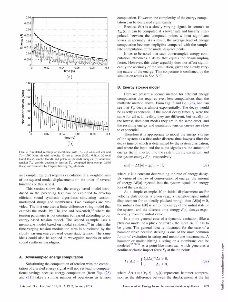
Figure 2 shows a synthetic example of a tension-

modulated rectangular membrane, obtained from the same

model of Fig. 1(b). The energies, computed from Eqs. (28)

and (31), are plotted in Fig. 2(a). The energy-based estima-

tion of Tqs is plotted in Fig. 2(b), along with the nonlinear

tension TNL. As a term of comparison, the figure also plots

an estimate of Tqs [dotted line in Fig. 2(b)] obtained by

applying a lowpass filter to TNL.The kinetic and potential energies oscillate in antiphase,

and the total energy is a slowly decaying signal as expected.

Note that the total energy is not exactly a monotonically

decreasing signal and exhibits small oscillations instead.

This is due to the fact that the potential energy Ep in Eq. (31)

has been derived in the linear regime, discarding the effects

of tension modulation.

The example shows that the quasistatic tension can be

accurately computed from the energy. Similar plots are

obtained for the string and the circular membrane.

V. EFFICIENT SOUND SYNTHESIS

As already mentioned, computing the nonlinear tension

component TNL at sample rate is an expensive operation. As


Au

tho

r's

com

plim

enta

ry c

op

y

an example, Eq. (17) requires calculation of a weighted sum

of the squared modal displacements (in the order of several

hundreds or thousands).

This section shows that the energy-based model intro-

duced in the preceding text can be exploited to develop

efficient sound synthesis algorithms simulating tension-

modulated strings and membranes. Two examples are pro-

vided. The first one uses a finite-difference string model that

extends the model by Chaigne and Askenfelt,32 where the

tension parameter is not constant but varied according to our

energy-based tension model. The second example uses a

membrane model based on modal synthesis26 in which the

time-varying tension modulation term is substituted by the

slowly varying energy-based quasi-static tension. The same

ideas could also be applied to waveguide models or other

sound synthesis paradigms.

A. Downsampled energy computation

Substituting the computation of tension with the compu-

tation of a scaled energy signal will not yet lead to computa-

tional savings because energy computation [from Eqs. (28)

and (31)] takes a similar number of operations as tension

computation. However, the complexity of the energy compu-

tation can be decreased significantly.

Because E(t) is a slowly varying signal, in contrast to

TNL(t), it can be computed at a lower rate and linearly inter-

polated between the computed points without significant

losses in accuracy. As a result, the average load of energy

computation becomes negligible compared with the sample-

rate computation of the modal displacements.

It has to be noted that such downsampled energy com-

putation introduces a delay that equals the downsampling

factor. However, this delay arguably does not affect signifi-

cantly the accuracy of the simulation, given the slowly vary-

ing nature of the energy. This conjecture is confirmed by the

simulation results in Sec. V C.

B. Energy storage model

Here we present a second method for efficient energy

computation that requires even less computations than the

multirate method above. From Fig. 2 and Eq. (26), one can

see that Tqs decays almost exponentially. The decay would

be exactly exponential if the modal decay times sg were the

same for all g. In reality, they are different, but usually for

the lowest, dominant modes they are in the same order, and

the resulting energy and quasistatic tension curves are close

to exponential.

Therefore it is appropriate to model the energy storage

of the system as a first-order discrete-time lowpass filter the

decay time of which is determined by the system dissipation,

and where the input and the ouput signals are the amount of

energy DE n½ � injected into the system during excitation, and

the system energy E n½ �, respectively:

E½n� ¼ DE½n� þ gE½n� 1�; (37)

where g is a constant determining the rate of energy decay.

By virtue of the law of conservation of energy, the amount

of energy DE n½ � injected into the system equals the energy

loss of the excitation.

As a simple example, if an initial displacement and/or

velocity distribution is given (e.g., a triangle-shaped initial

displacement for an ideally plucked string), then DE n½ � ¼ 0;the initial value E 0½ � is set to the energy of the initial state of

the system, and the discrete-time energy E n½ � decays expo-

nentially from the initial value.

In a more general case of a dynamic excitation (like a

physical model of a pluck or strike), the input DE n½ � has to

be given. The general idea is illustrated for the case of a

hammer strike because striking is one of the most common

forms of excitation in string and membrane instruments. A

hammer or mallet hitting a string or a membrane can be

modeled32,38,39 as a point-like mass mh, which generates a

nonlinear elastic impact force Fh at the hit point:

FhðDzÞ ¼khðDzÞahDz > 0;

0 Dz 0;

�(38)

where Dz tð Þ ¼ z xh; tð Þ � zh tð Þ represents hammer compres-

sion as the difference between the displacement at the hit

FIG. 2. Simulated rectangular membrane with (Lx, Ly)¼ (32,25) cm and

T0¼ 1500 N/m, hit with velocity 10 m/s at point (0.3Lx, 0.1Ly); (a) total

(solid thick), kinetic (solid), and potential (dashed) energies; (b) nonlinear

tension TNL (solid), quasistatic tension Tqs computed from energy (solid

thick) and estimated by lowpass filtering TNL (dashed).


Au

tho

r's

com

plim

enta

ry c

op

y

point xh and the hammer displacement zh, kh is the force

stiffness, and the exponent ah depends on the local geometry

around the contact area. The hammer energy during contact

is

Eh ¼1

2mh _z2

h þ khDzahþ1

ah þ 1; (39)

and can therefore be computed at every time instant. The

energy input to the system is then the energy change of the

hammer:

DE½n� ¼ �ðEh½n� � Eh½n� 1�Þ: (40)

In summary, the proposed energy storage model realizes a

tension-modulated string or membrane model with essen-

tially the same computational load as that of a linear model.

The only required additional sample-rate operations are the

sums and multiplications needed to

(1) Compute DE n½ � by Eqs. (39) and (40) during contact.

(2) Estimate E n½ � by the filter of Eq. (37).

(3) Compute Tqs n½ � by Eq. (36).

For a lossy excitation mechanism, such as a hysteretic

hammer,40,41 the dissipation of the damping element has to

be subtracted from the energy input DE n½ �.Figure 3 shows the log energy decay of a circular mem-

brane [from the same model of Fig. 1(b)], struck at a point

rh¼ 0.5R with impact velocity 20 m/s. An almost linear

decay is observed on a logarithmic scale as expected. The

dashed line is the energy computed by the energy storage

model of Eq. (37) and the hammer energy of Eq. (39). The gparameter of Eq. (37) was estimated by fitting a line on the

log energy plot, although it can also be estimated from the

decay times of the first modes. The small discrepancy

between the actual and modeled energies is most probably

due to the fact that modeling the energy loss by Eq. (37) also

during excitation is only a rough approximation.

Compared with the downsampled energy computation,

the energy storage model leads to lower computational com-

plexity. On the other hand, it requires the formulation of the

energy of the exciter. In general, for such excitations where

the energy can be expressed in a closed form (like for the

simple pluck and impact models used in this paper), this lat-

ter method should be used because of its computational

efficiency.

C. Results

Simulation results are summarized in the spectrograms

of Figs. 4 and 5. All have been obtained through short-time

Fourier transform (STFT) analysis, with a frame length and

a hop-size of 8192 and 128 samples, respectively (with sam-

pling rate of 44.1 kHz). The energy spreading in frequency

observed during the attack is the effect of the STFT analysis

on the exponentially decaying modal frequencies.

FIG. 3. Log-scale energy decay of a simulated circular membrane excited

by an impact force: membrane energy (solid line) and estimated energy

computed by the energy storage model of Eq. (37) (dashed line).

FIG. 4. Spectrograms (with SPL in dB) of a simulated string; (a) complete

model using nonlinear tension TNL of Eq. (17); (b) efficient model using qua-

sistatic tension Tqs, computed from energy via Eq. (36), with a downsam-

pling factor of 32; (c) efficient model using the energy storage model of Eq.

(37) to compute the quasistatic tension Tqs.


Au

tho

r's

com

plim

enta

ry c

op

y

The three spectrograms in Fig. 4 are all obtained by

plucking the same finite-difference string model of Fig. 1(a).

Here the triangle-shaped initial displacement distribution has

a peak value of 10 mm. Figure 4(a) corresponds to earlier

tension modulation models, where the tension TNL is com-

puted from the string displacement by the discretized version

of Eq. (4). The spectrogram in Fig. 4(b) instead has been

obtained by approximating TNL with Tqs, estimated from the

string energy according to Eq. (36), and computed with a

downsampling factor 32, i.e., every 32/44.1 � 0.73 ms.

Finally, the spectrogram in Fig. 4(c) has been obtained by

approximating the string energy by the energy storage model

of Eq. (37) and by computing Tqs from this estimated

energy.

Figure 5 shows three spectrograms of a rectangular

membrane, all obtained by striking the same modal-based

membrane model of Fig. 2. Here the impact velocity is 20

m/s, which is close to the highest dynamic levels in drum

playing.33

According to the spectrograms and informal listening

tests, the results of the different models are basically indis-

tinguishable for the rigidly terminated string. This is

expected from theory because mode coupling does not occur

for rigid terminations and only the quasistatic part of tension

variation has an effect, as discussed in Sec. IV A.

This is not exactly the case for the membrane, probably

due to the mode coupling that can still arise in the full model

even for rigid boundaries (see Sec. IV A). However, the

main goal of synthesizing pitch glides correctly is still

accomplished. Compared with the full tension modulation

model, the efficient models trade a less relevant phenomenon

(some mode coupling) for significantly lower computational

complexity. Formal listening tests on perceptual differences

of the models are out of the scope of this paper and are left

for future research. Interested readers may listen to the

sound examples at http://www.dei.unipd.it�avanzini/demos/jasa2011/.

VI. CONCLUSIONS

This paper has presented a unified formulation to the

tension modulation problem for strings and membranes. For

the membrane, circular and rectangular geometries were

considered.

By expressing both tension and energy of vibration as

functions of modal amplitudes, it was shown that the quasi-

static (short-time average) part of tension variation is line-

arly proportional to the energy of the system. This allowed

the development of efficient tension-modulated sound syn-

thesis models that simulate pitch glides in musical instru-

ments at a negligible additional computational cost to that

incurred by linear string and membrane models. The effi-

ciency comes from the fact that the system energy is esti-

mated at a significantly lower computational complexity

compared with tension calculation.

For this, two methods were proposed. The first one com-

putes energy at a lower sampling rate, and uses linear inter-

polation in between. The second one models the energy

decay by a first order lowpass filter the input of which is the

energy loss of the exciter (e.g., the hammer). Both methods

allow the accurate synthesis of pitch glides and require lower

computational complexity compared with earlier tension-

modulated models.

ACKNOWLEDGMENTS

The work of Balazs Bank was supported by the EEA

and Norway Grants and the Zoltan Magyary Higher Educa-

tion Foundation. We are thankful to Dr. Stefan Bilbao, Dr.

Federico Fontana, and the anonymous reviewers for their

helpful comments.

FIG. 5. Spectrograms (with SPL in dB) of a simulated rectangular mem-

brane; (a) complete model using nonlinear tension TNL of Eq. (17); (b) effi-

cient model using quasistatic tension Tqs, computed from energy via

Eq. (36), with a downsampling factor of 32; (c) efficient model using the

energy storage model of Eq. (37) to compute the quasistatic tension Tqs.


Au

tho

r's

com

plim

enta

ry c

op

y

1B. Bank, “Physics-based sound synthesis of string instruments including

geometric non-linearities,” Ph.D. thesis, Budapest University of Technol-

ogy and Economics, Budapest, 2006.2S. Bilbao, “Conservative numerical methods for nonlinear strings,”

J. Acoust. Soc. Am. 118, 3316–3327 (2005).3S. Bilbao, Numerical Sound Synthesis—Finite Difference Schemes andSimulation in Musical Acoustics (Wiley, Chichester, 2009), Chap. 8, pp.

221–247.4C. Erkut, M. Karjalainen, P. Huang, and V. Valimaki, “Acoustical analysis

and model-based sound synthesis of the kantele,” J. Acoust. Soc. Am. 112,

1681–1691 (2002).5N. H. Fletcher and T. D. Rossing, The Physics of Musical Instruments(Springer-Verlag, New York, 1991), Chap. 18, pp. 516–517.

6G. F. Carrier, “On the nonlinear vibrations problem of elastic string,”

Quart. J. Appl. Math. 3, 157–165 (1945).7M. Karjalainen, J. Backman, and J. Polkki, “Analysis, modeling, and real-

time sound synthesis of the kantele, a traditional finnish string

instrument,” Proceedings of the IEEE International Conference on Acous-tics, Speech and Signal Processing, Minneapolis, MN (1993), Vol. 1, pp.

229–232.8J. O. Smith III, “Principles of digital waveguide models of musical

instruments,” in Applications of Digital Signal Processing to Audio andAcoustics, edited by M. Kahrs and K.-H. Brandenburg (Kluwer Academic

Publishers, New York, 1998), pp. 417–466.9T. Tolonen, V. Valimaki, and M. Karjalainen, “Modeling of tension modu-

lation nonlinearity in plucked strings,” IEEE Trans. Speech Audio Pro-

cess. 8, 300–310 (2000).10J. Pakarinen, V. Valimaki, and M. Karjalainen, “Physics-based methods

for modeling nonlinear vibrating strings,” Acust. Acta Acust. 91, 312–325

(2005).11V. Valimaki, J. Pakarinen, C. Erkut, and M. Karjalainen, “Discrete-time

modelling of musical instruments,” Rep. Prog. Phys. 69, 1–78 (2006).12J.-M. Adrien, “The missing link: Modal synthesis,” in Representations of

Musical Signals, edited by G. De Poli, A. Piccialli, and C. Roads (MIT

Press, Cambridge, MA, 1991), pp. 269–297.13R. Rabenstein and L. Trautmann, “Digital sound synthesis of string instru-

ments with the functional transformation method,” Signal Process. 83,

1673–1688 (2003).14L. Trautmann and R. Rabenstein, Digital Sound Synthesis by Physical

Modeling Using the Functional Transformation Method (Kluwer Aca-

demic/Plenum Publishers, New York, 2003), Chap. 5, pp. 95–130.15S. Bilbao, “Modal type synthesis techniques for nonlinear strings with an

energy conservation property,” in Proceedings of the International Confer-ence on Digital Audio Effects (DAFx-04), Naples, Italy (2004), pp. 119–124.

16S. Bilbao, “Energy-conserving finite difference schemes for tension-

modulated strings,” in Proceedings on the IEEE International Conferenceon Acoustics, Speech and Signal Processing, Montreal, Quebec (2004),

pp. 285–288.17S. A. Van Duyne and J. O. Smith III, “The 2-D digital waveguide mesh,”

in Proceedings of the IEEE Workshop on Applied Signal Processing toAudio and Acoustics (WASPAA93), New Paltz, NY (1993), pp. 177–180.

18F. Fontana and D. Rocchesso, “Signal-theoretic characterization of wave-

guide mesh geometries for models of two-dimensional wave propagation

in elastic media,” IEEE Trans. Speech Audio Process. 9, 152–161 (2001).19L. Savioja and V. Valimaki, “Interpolated rectangular 3-D digital wave-

guide mesh algorithms with frequency warping,” IEEE Trans. Speech

Audio Process. 11, 783–790 (2003).

20S. Petrausch and R. Rabenstein, “Tension modulated nonlinear 2D

models for digital sound synthesis with the functional transformation

method,” in Proceedings of the European Signal Processing Conference(EUSIPCO2005), Antalya, (2005).

21C. H. Jenkins and J. W. Leonard, “Nonlinear dynamic response of mem-

branes: State of the art,” Appl. Mech. Rev. 44, 319-328 (1991).22C. H. Jenkins, “Nonlinear dynamic response of membranes: State of the

art—update,” Appl. Mech. Rev. 48, S41–S48 (1996).23J. S. Rao, Dynamics of Plates (Marcel Dekker, New York, 1999), Chap. 6,

pp. 179–227.24S. Bilbao, “Sound synthesis for nonlinear plates,” in Proceedings of the

International Conference on Digital Audio Effects (DAFx-05) Madrid

(2005), pp. 243–248.25S. Bilbao, “A family of conservative finite difference schemes for the dy-

namical von Karman plate equations,” Numer. Methods Partial Differ.

Equ. 24, 193–216 (2008).26F. Avanzini and R. Marogna, “A modular physically-based approach to

the sound synthesis of membrane percussion instruments,” IEEE Trans.

Audio Speech Lang. Process. 18, 891–902 (2010).27R. Marogna and F. Avanzini, “Physically based synthesis of nonlinear cir-

cular membranes,” in Proceedings of the International Conference onDigital Audio Effects (DAFx-09) Como (2009), pp. 373–379.

28H. M. Berger, “A new approach to the analysis of large deflections of

plates,” ASME J. Appl. Mech. 22, 465–472 (1955).29Zs. Garamvolgyi, “Physics-based modeling of membranes for sound syn-

thesis applications,” Master’s thesis, Budapest University of Technology

and Economics, Hungary (2008).30B. Bank, “Energy-based synthesis of tension modulation in strings,” in

Proceedings of the International Conference on Digital Audio Effects(DAFx-09) Como (2009), pp. 365–372.

31R. Marogna, F. Avanzini, and B. Bank, “Energy based synthesis of tension

modulation in membranes,” in Proceedings of the International Confer-ence on Digital Audio Effects (DAFx-10) Graz (2010), pp. 102–108.

32A. Chaigne and A. Askenfelt, “Numerical simulations of piano strings.

I. A physical model for a struck string using finite difference methods,”

J. Acoust. Soc. Am. 95, 1112–1118 (1994).33S. Dahl, “Playing the accent—comparing striking velocity and timing in

an ostinato rhythm performed by four drummers,” Acust. Acta Acust. 90,

762–776 (2004).34N. H. Fletcher and T. D. Rossing, The Physics of Musical Instruments

(Springer-Verlag, New York, 1991), Chap. 2, p. 38.35N. H. Fletcher and T. D. Rossing, The Physics of Musical Instruments

(Springer-Verlag, New York, 1991), Chap. 3, pp. 66–70.36K. A. Legge and N. H. Fletcher, “Nonlinear generation of missing modes

on a vibrating string,” J. Acoust. Soc. Am. 76, 5–12 (1984).37P. M. Morse, Vibration and Sound, 2nd edition (McGraw-Hill, New York,

1948), Chap. 3, pp. 89–91.38X. Boutillon, “Model for piano hammers: Experimental determination and

digital simulation,” J. Acoust. Soc. Am. 83, 746–754 (1988).39L. Rhaouti, A. Chaigne, and P. Joly, “Time-domain modeling and numeri-

cal simulation of a kettledrum,” J. Acoust. Soc. Am. 105, 3545–3562

(1999).40K. H. Hunt and F. R. E. Crossley, “Coefficient of restitution interpreted

as damping in vibroimpact,” ASME J. Appl. Mech. 42, 440–445

(1975).41A. Stulov, “Hysteretic model of the grand piano felt,” J. Acoust. Soc. Am.

97, 2577–2585 (1995).


Au

tho

r's

com

plim

enta

ry c

op

y

Documents

Efficient synthesis of tension modulation in strings and membranes based on energy estimation