Embed Size (px)
Citation preview
Olivier RAMARÉ
Eigenvalues in the large sieve inequality, IITome 22, no 1 (2010), p. 181-195.
<http://jtnb.cedram.org/item?id=JTNB_2010__22_1_181_0>
© Université Bordeaux 1, 2010, tous droits réservés.
L’accès aux articles de la revue « Journal de Théorie des Nom-bres de Bordeaux » (http://jtnb.cedram.org/), implique l’accordavec les conditions générales d’utilisation (http://jtnb.cedram.org/legal/). Toute reproduction en tout ou partie cet article sousquelque forme que ce soit pour tout usage autre que l’utilisation àfin strictement personnelle du copiste est constitutive d’une infrac-tion pénale. Toute copie ou impression de ce fichier doit contenir laprésente mention de copyright.
cedramArticle mis en ligne dans le cadre du
Centre de diffusion des revues académiques de mathématiqueshttp://www.cedram.org/
Journal de Théorie des Nombresde Bordeaux 22 (2010), 181-195
Eigenvalues in the large sieve inequality, II
par Olivier RAMARÉ
Résumé. Nous explorons numériquement les valeurs de la formehermitienne ∑
q≤Q
∑a mod ∗q
∣∣∣∑n≤N
ϕne(na/q)∣∣∣2
lorsque N =∑
q≤Q φ(q). Nous améliorons la majoration actuelleet exhibons un graphique conjectural de la distribution asympto-tique de ses valeurs propres en exploitant des résultats de calculsintensifs. L’une des conséquences est que la distribution asympto-tique existe probablement mais n’est pas absolument continue parrapport à la mesure de Lebesgue.
Abstract. We explore numerically the eigenvalues of the her-mitian form ∑
q≤Q
∑a mod ∗q
∣∣∣∑n≤N
ϕne(na/q)∣∣∣2
when N =∑
q≤Q φ(q). We improve on the existing upper bound,and produce a (conjectural) plot of the asymptotic distributionof its eigenvalues by exploiting fairly extensive computations. Themain outcome is that this asymptotic density most probably existsbut is not continuous with respect to the Lebesgue measure.
1. IntroductionIn [9], we explored numerically as well as theoretically the distribution
of the eigenvalues of the hermitian form
(1.1)∑q≤Q
∑a mod ∗q
∣∣∣∑n≤N
ϕne(na/q)∣∣∣2
when Q2 is close to N . Bounds for this hermitian form are of utmost im-portance for arithmetical uses and are the core of what is loosely refered to
Manuscrit reçu le 4 octobre 2008.Mots clefs. Large sieve inequality, circle method, Jackson polynomials, Hausdorff moment
problem.Classification math. 11L03, 11L07, 11L26, 30E05, secondary : 41A10, 41A17.
182 Olivier Ramaré
as "the large sieve" and we refer the reader to [7] and [1] for more detailson this subject. Let us assume that
(1.2) N = Φ(Q) =∑q≤Q
φ(q)
and let us denote by (λi)1≤i≤N be its eigenvalues. We produced graphicsin [9] showing that the sequence of functions of λ defined by(1.3) D(N,Q, λ) = #{i/λi ≤ λN}/Nseems to converge. The question has been asked as to the shape of thedensity involved and whether one could produce a graphical candidate forthis density. The underlying idea is also that one may hope to guess whatthis density should be from its shape. Note that the large sieve inequalitytells us that these eigenvalues are not more than N + Q2, so that λ isconstrained to lie in [0, L], with practically L = 3.5. See also section 2 onthis paper for the upper bound L ≤ 3.548 and section 3 for a hint as towhat the actual value can be.
Producing such a diagram is however more difficult than its seems. In-deed, assuming this density to be continuous, we can approximate it bythe number of eigenvalues (renormalized by being divided by N) lying ina given interval. However, when this interval is too small, this number willonly be 0 or 1. We thus should guess what is the proper length to be used. Itis tempting to select intervals of length about 1/
√N , but N being between
100 and 500, this means having only 10 to 20 intervals at our disposal.This also means computing all the eigenvalues while only using very partialinformation concerning them.
We decided to follow a more direct approach: since the computation ofthe eigenvalues in fact relied on computing powers of our matrix, say M ,in order to build its characteristic polynomial, we set to compute the traceof these powers but only to a limited power h ≤ H = 100. This also meansthat we have been able to increase noticeably the size of our matrices: thelargest Q for which we have computed all the eigenvalues is Q = 40, andthis means 490 eigenvalues, while we computed the 100th first momentsfor Q = 70, using a precision of 110 digits. This means handling matricesof size 1 494 × 1 494. These computations are somewhat more detailed insection 3. We then try to guess the form of the density. We have thus accessto the quantities ∫ L
0thdD(t) (0 ≤ h ≤ H)
and we aim at recovering∫I dD(t)/|I| for intervals I as small as possible.
We approximate in fact dD(x)/dx by
(1.4)∫ L
0P (x, t)dD(t)/
∫ L
0P (x, t)dt
Eigenvalues in the large sieve inequality, II 183
where P (x, t) is a polynomial of degree ≤ n and which has a sharp peakat x. We take n = H. Deciding of which polynomials to take is again aproblem. We opted for a solution involving Jackson polynomials (recalledthereafter). A similar problem, but with fairly smooth densities, has alreadybeen considered in [3] where the author resorts to Bernstein polynomials.Jackson polynomials provide a better polynomial approximation, in partic-ular with densities that have a low level of regularity. These polynomialshave the advantage of being non-negative, while having a sharp peak atfairly well-spaced points (this is false close to the edge of the range, butour distribution is very small there). To produce a diagram, we proceededas follows
(1) we took the n/2 points xk = 2kL/n for k from 0 to n/2.(2) The points x∗k = 2(xk/L)− 1 are now well-spaced over [−1, 1].(3) For each k, select ` such that
cos2π`n+ 1
≥ x∗k > cos2π(`+ 1)n+ 1
and take a linear interpolation of the relevant Jackson polynomials:
P ∗(x∗k, t) = λK`,n(t) + (1− λ)K`+1,n(t)
where
λ =x∗k − cos 2π(`+1)
n+1
cos 2π`n+1 − cos 2π(`+1)
n+1
.
(4) We finally choose P (xk, t) = P ∗(x∗k, 2t− 1).Since we have all these moments at our disposal, we decided to investi-
gate them as well. The reader will see in section 3 that they behave veryregularly. We thus decided to produce a numerical fit. If a distribution canbe written as dD(t) = δ(t)dt with a smooth enough function δ, then thesemoments should behave like A+B(Log h)/h+O((Log2 h)/h2). This is notwhat we obtained, see section 3 for more details.
2. On the largest eigenvalue when N = Φ(Q)
In his lectures on sieve [10], Selberg announced that the largest eigenvalueof (1.1) is indeed ≤ (1− ε)(N +Q2) for some ε > 0 and when N = Φ(Q),see (1.2). However, he provided no numerical values for ε and this is the aimof this section. We recall the path proposed by Selberg. Let F1 be a smoothfunction on the real line that majorizes the characteristic function of theinterval [1, N ] and such that its Fourier transform F1 vanishes when theargument is ≥ Q−2 in absolute value. We also assume that this functiondecreases fast enough at both infinities to ensure the convergence of the
184 Olivier Ramaré
quantities appearing in the Poisson summation formula. We write
∑q≤Q
∑a mod ∗q
∣∣∣S(a/q)∣∣∣2 =
∑n≤N
ϕn∑q≤Q
∑a mod ∗q
S(a/q)e(na/q)
with S(a/q) =∑n ϕne(na/q), and we apply Cauchy’s inequality. This leads
to∑q≤Q
∑a mod ∗q
∣∣∣S(a/q)∣∣∣22
≤∑n≤N|ϕn|2
∑1≤n≤N
∣∣∣ ∑q≤Q,
a mod ∗q
S(a/q)e(na/q)∣∣∣2
≤∑n≤N|ϕn|2
∑n∈Z
F1(n)∣∣∣ ∑
q≤Q,a mod ∗q
S(a/q)e(na/q)∣∣∣2.
We expand the last square:
∑n≤N|ϕn|2
∑q≤Q,
a mod ∗q
∑q′≤Q,
a′ mod ∗q′
S(a/q)S(a′/q′)∑n∈Z
F1(n)e(n(a/q − a′/q′))
≤∑n≤N|ϕn|2
∑q≤Q,
a mod ∗q
∑q′≤Q,
a′ mod ∗q′
S(a/q)S(a′/q′)∑m∈Z
F1(m− (a/q− a′/q′))
by Poisson summation formula. By our assumption, only m = 0 and a/q =a′/q′ survive in the inner summation. This gives us
∑q≤Q
∑a mod ∗q
∣∣∣S(a/q)∣∣∣2 ≤ F1(0)
∑n≤N|ϕn|2.
Our problem is thus to minimize the value of F1(0). Note that the functionF (u) = F1(Q2u+N/2) verifies F (x) = Q2F1(x/Q2)e(xN/2). We translateour conditions on F :
(1) F (x) = 0 when |x| ≥ 1;(2) F (u) ≥ 0 for all u ∈ R;(3) F (u) ≥ 1 when 2|u| ≤ N/Q2.
We take F of the shape
(2.1) F (u) =∫ ∞−∞
∫ 1
0G(v)G(v − x)dv e(−xu)dx
Eigenvalues in the large sieve inequality, II 185
for some real-valued function G with support on [0, 1]. As a consequence,the function x 7→
∫ 10 G(v)G(v − x)dv has support on [−1, 1], so that
F (u) =∫ 1
−1
∫ 1
0G(v)G(v − x)dv e(−xu)dx
=∫ 1
0G(v)e(−vu)dv
∫ 1
−1G(v − x)e((v − x)u)dx
=∣∣∣∫ 1
0G(v)e(−vu)dv
∣∣∣2.This representation thus ensures us that F (x) = 0 when |x| ≥ 1 and thatF (u) ≥ 0 for all u ∈ R. Our problem reduces to minimizing
F (0) =∫ 1
0G(v)2dv =
∫ ∞−∞|G(u)|2du
when ∣∣∣∫ 1
0G(v)e(−vu)dv
∣∣∣ ≥ 1 (|u| ≤ δ)
where δ = N/(2Q2). In our case, δ is asymptotic to 3/(2π2) which is prettysmall! We want |G(u)| to be as close to the characteristic function of theinterval [−δ, δ] as is possible and this tells us that F (0) ≥ 2δ. We have notbeen able to solve this extremal problem, so we decided to run experimentsby taking G to be a polynomial. First note the formula
(2.2) Ek(u) =∫ 1
0vke(−vu)dv =
k!e(−u)(2iπu)k+1
e(u)−∑
0≤`≤k
(2iπu)`
`!
.Proof: The formula is valid for k = 0. Assume it has been proved for k.An integration by parts yields∫ 1
0vk+1e(−vu)dv =
e(−u)−2iπu
+(k + 1)2iπu
Ek(u)
=e(−u)−2iπu
+(k + 1)!e(−u)
(2iπu)k+2
e(u)−∑
0≤`≤k
(2iπu)`
`!
=
(k + 1)!e(−u)(2iπu)k+2
e(u)−∑
0≤`≤k
(2iπu)`
`!− (2iπu)k+1
(k + 1)!
as required. � � �
On taking simply G0(v) = 1, we already get an improvement on the usuallarge sieve inequality: the largest eigenvalues is less than 3.552 · N if Q islarge enough, instead of (1 +π2/3)N ≤ 4.290 ·N . The choice 1 + v(1− v)/2yields the bound 3.548 ·N . Note that its L2-norm is
√47/40 and not 1; we
set G1(v) = (1 + v(1 − v)/2)/√
47/40. As a matter of fact, we tried every
186 Olivier Ramaré
polynomial 1 + a1v+ a2v2 + a3v
3 + a4v4 with the ai’s ranging {2 k
20 − 1, k ∈{0, . . . , 20}}.
We explored the situation further, but on restricting our attention topolynomials of shape 1+b1v(1−v)+b2v2(1−v)2+b3v3(1−v)3+b4v4(1−v)4
with the bi’s ranging {2 k20 − 1, k ∈ {0, . . . , 20}}. We found the polynomial
1+ 12v(1−v)+ 3
10v4(1−v)4 (of L2-norm
√8577013/7293000) which leads to a
very marginal improvement: 3.547 411 612·N instead of the 3.547 411 644·Nobtained with G1(v). We further set
(2.3) G2(v) =(1 + 1
2v(1− v) + 310v
4(1− v)4)/√
8577013/7293000.
We record some more formulae in case they be of use to the reader. Withp = 2πu, we have
4740|G1(u)|2 =
4(1 + p4)(1− cos p)− 4p3 sin p+ p2(9− 7 cos p)− 4p sin p2p6
with |G1(0)|2 = 845/846 = 0.998 817 . . . . Concerning G2, we get
85770137293000
50p18|G2(u)|2
= p(p6 − 288p2 + 12096)(5p8 + 5p6 + 36p4 − 6480p2 + 60480) sin p
+ (10p8 − 5p7 + 10p6 + 72p4 + 1440p3 − 12960p2 − 60480p+ 120960)
(10p8 + 5p7 + 10p6 + 72p4 − 1440p3 − 12960p2 + 60480p+ 120960) cos p
+ 100p16 + 225p14 + 1540p12 − 272160p10 + 2769984p8 + 2626560p6
+ 11197440p4 + 522547200p2 + 14631321600
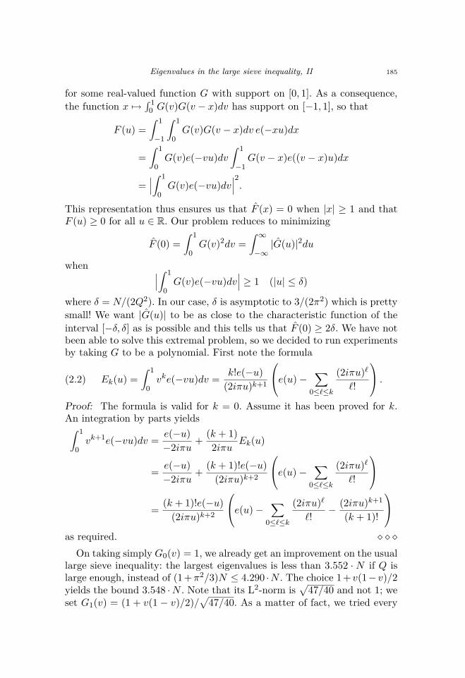
and |G2(0)|2 = 6296503928/6304104555 = 0.998 794 · · · .The plot corresponding to G0 starts above the ones of G1 and G2, and
dips slightly below around 0.1.the one of G1 while the one of G2 is indis-tinguishable from the one of G1.
The above proof can easily be generalized to get the following Theorem:
Theorem 2.1. When X be a subset of R/Z such that min ‖x − x′‖ ≥ δwhere ‖y‖ is the distance on the unit circle. Let us assume that Nδ ≤ 9/10.We have ∑
x
∣∣∣∑n≤N
ϕne(nx)∣∣∣2 ≤∑
n
|ϕn|2(1 + |G2(Nδ)|−2)δ−1
where (ϕn) is any complex sequence.
In fact, when Nδ is small, at least when Nδ ≤ 1/10, it is better to useG0 instead of G2.
Eigenvalues in the large sieve inequality, II 187
1
1.1389e-53
0.001 1
Figure 1. Plot of the modulus square of the Fourier trans-form of G0, G1 and G2.
In particular, when N = Φ(Q) and Q is large enough, we have∑q≤Q
∑a mod ∗q
∣∣∣∑n≤N
ϕne(na/q)∣∣∣2 ≤ 3.547 411 612 ·N ·
∑n
|ϕn|2.
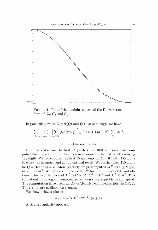
3. On the momentsOur first datas are the first H (with H = 100) moments. We com-
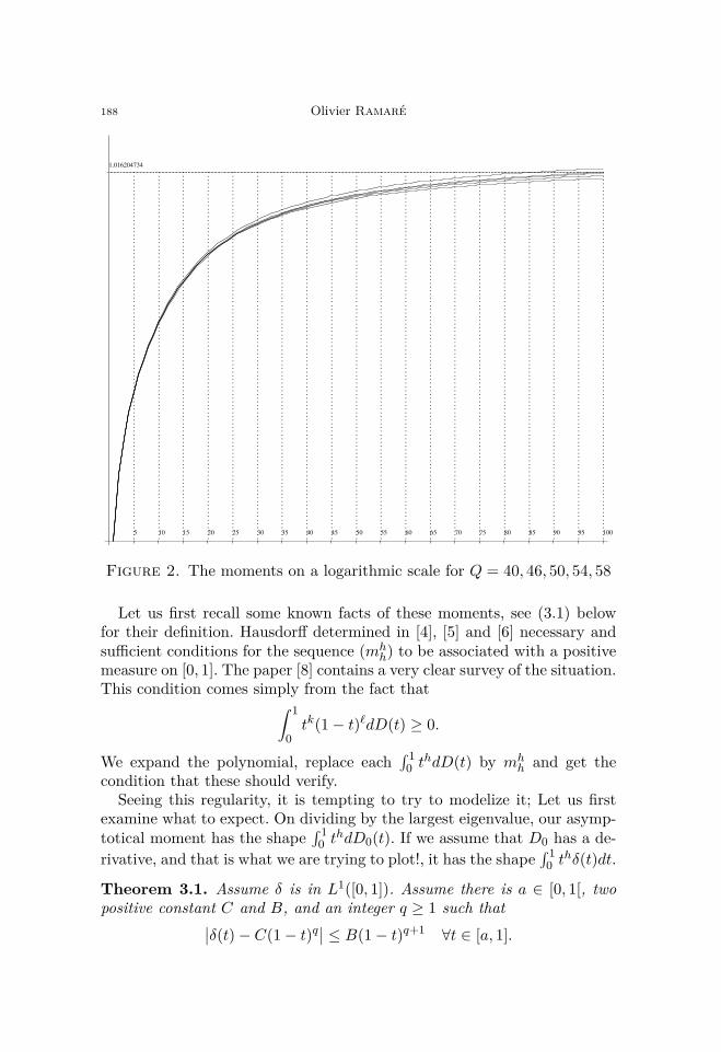
puted them by computing the successive powers of the matrix M , on using100 digits. We recomputed the first 15 moments for Q = 62 with 150 digitsto check the accuracy and got an optimal result. We further used 110 digitsfor Q = 66 and Q = 70. More precisely, we precomputedM2k for 0 ≤ k ≤ 6,as well as M3. We then computed each Mh for h a multiple of 4, and ob-tained this way the trace of Mh, Mh ×M , Mh ×M2 and Mh ×M3. Thisturned out to be a good compromise between storage problems and speed.The computation have been run GP/PARI with compiled scripts via GP2C.The scripts are available on request.
We show below a plot of
h 7→ Log(trMh/Nh+1).(h ≥ 1)
A strong regularity appears.
188 Olivier Ramaré
5 10 15 20 25 30 35 40 45 50 55 60 65 70 75 80 85 90 95 100
1.016204734
Figure 2. The moments on a logarithmic scale for Q = 40, 46, 50, 54, 58
Let us first recall some known facts of these moments, see (3.1) belowfor their definition. Hausdorff determined in [4], [5] and [6] necessary andsufficient conditions for the sequence (mh
h) to be associated with a positivemeasure on [0, 1]. The paper [8] contains a very clear survey of the situation.This condition comes simply from the fact that∫ 1
0tk(1− t)`dD(t) ≥ 0.
We expand the polynomial, replace each∫ 10 t
hdD(t) by mhh and get the
condition that these should verify.Seeing this regularity, it is tempting to try to modelize it; Let us first
examine what to expect. On dividing by the largest eigenvalue, our asymp-totical moment has the shape
∫ 10 t
hdD0(t). If we assume that D0 has a de-rivative, and that is what we are trying to plot!, it has the shape
∫ 10 t
hδ(t)dt.
Theorem 3.1. Assume δ is in L1([0, 1]). Assume there is a ∈ [0, 1[, twopositive constant C and B, and an integer q ≥ 1 such that∣∣δ(t)− C(1− t)q
∣∣ ≤ B(1− t)q+1 ∀t ∈ [a, 1].
Eigenvalues in the large sieve inequality, II 189
Then (∫ 1
0thδ(t)dt
)1/h= 1− qLog h
h+
Log(Cq!)h
+O((Log h)2/h2).
Proof: Indeed, an integration by parts yields readily∫ 1
0th(1− t)`dt =
`!h!(h+ `+ 1)!
and thus∫ 1
0thδ(t)dt =
∫ 1
athδ(t)dt+
∫ a
0thδ(t)dt
= C
∫ 1
0th(1− t)qdt
+O∗(B
∫ 1
0th(1− t)q+1dt+ ah(C +B + ‖δ‖1)
)=
Cq!h!(h+ q + 1)!
+O∗(B(q + 1)!h!
(h+ q + 2)!ah(C +B + ‖δ‖1)
).
We deduce from this that the moment to the power 1/h equals
( Cq!h!(h+ q + 1)!
)1/h(
1 +O(B(q + 1)h+ q + 2
+ (h+ q + 1)q+1ah))1/h
.
The logarithm of the main term is(Log(Cq!)− q Log h−
∑1≤`≤q+1
Log(1 +
`
h
))/h
which is (Log(Cq!) − q Log h + O(1/h))/h while the error term is simply1 +O(1/h2). The theorem follows readily.
� � �
This theorem says in essence that having a mild regularity throughoutthe interval and a somewhat stronger one near to the largest point of thesupport of our distribution are enough to ensure a convergence of the mo-ments in (Log h)/h. Having this in mind, we tried to fit the real curve witha regular one of equation h 7→ A + B(Log h)/h. Let us first recall rapidlyhow this can be achieved via a least squares estimate. We set
(3.1) mh(N) =
∑1≤k≤N
λhi /Nh+1
1/h
.
190 Olivier Ramaré
We should minimize∑1≤h≤H
(mh(N)−
∑i
Aifi(h))2 =
∑1≤h≤H
mh(N)2
− 2∑i
Ai∑
1≤h≤Hmh(N)fi(h) +
∑1≤h≤H
(∑i
Aifi(h)
)2
for some chosen functions fi. In our main example, we take only the twofunctions f1(h) = 1 and f2(h) = Log(h)/h. The vanishing of the partialderivatives in Ai of the above quadratic form leads to a linear system:
∀i,∑j
Aj∑
1≤h≤Hfi(h)fj(h) =
∑1≤h≤H
mh(N)fi(h).
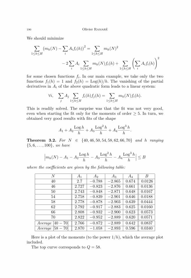
This is readily solved. The surprise was that the fit was not very good,even when starting the fit only for the moments of order ≥ 5. In turn, weobtained very good results with fits of the shape
A1 +A2Log hh
+A3Log2 h
h+A4
Log3 h
h.
Theorem 3.2. For N ∈ {40, 46, 50, 54, 58, 62, 66, 70} and h ranging{5, 6, . . . , 100}, we have
∣∣∣mh(N)−A1 −A2Log hh−A3
Log2 h
h−A4
Log3 h
h
∣∣∣ ≤ Bwhere the coefficients are given by the following table:
N A1 A2 A3 A4 B40 2.7 −0.788 −2.865 0.674 0.012646 2.727 −0.823 −2.876 0.661 0.013650 2.743 −0.848 −2.871 0.648 0.016754 2.758 −0.839 −2.901 0.646 0.018858 2.778 −0.878 −2.903 0.639 0.044462 2.792 −0.917 −2.883 0.625 0.016066 2.808 −0.932 −2.900 0.623 0.057370 2.822 −0.952 −2.889 0.620 0.0571
Average [40− 70] 2.766 −0.872 −2.889 0.642 0.0837Average [58− 70] 2.870 −1.058 −2.893 0.596 0.0340
Here is a plot of the moments (to the power 1/h), which the average plotincluded.
The top curve corresponds to Q = 58.
Eigenvalues in the large sieve inequality, II 191
5 10 15 20 25 30 35 40 45 50 55 60 65 70 75 80 85 90 95 100
2.790369037
Figure 3. The moments for Q = 40, 46, 50, 54, 58 and theaverage fit
The maximum of the average fit is obtained close to h = 500 and hasvalue 2.833 · · · . As a consequence, one may ask whether it is true that∑
q≤Q
∑a mod ∗q
∣∣∣∑n≤N
ϕne(na/q)∣∣∣2 ?≤ 3.2N
∑n
|ϕn|2 (N = Φ(Q)).
The graph we produce in the last section goes in favor of this guess. Thenumerical datas are however too flimsy to term that a conjecture, or toeven guess the optimal constant.
4. On Jackson’s polynomialsApproximation and interpolation of the circle. We essentially followthe notations of [11] and define for any non-negative integer n
(4.1) Kn(v) =2
n+ 1
(sin n+1
2 v
2 sin(v/2)
)2
=12
+1
n+ 1
∑1≤`≤n
(n+ 1− `) cos `v
192 Olivier Ramaré
as well as
(4.2) rk,n = r0,n +2πkn+ 1
where r0,n is an arbitrary real number. Note that Kn(0) = (n + 1)/2,Kn(v) ≥ 0 and
∫ 2π0 Kn(v)dv = 1/2. We define the Jackson polynomial of a
2π-periodic function f to be
(4.3) Jn(f, u) =2
n+ 2
∑0≤k≤n
f(rk,n
)Kn(u− rk,n
).
These polynomials are uniquely determined by the interpolation property:
(4.4) J(f, rk,n
)= f
(rk,n
), J ′
(f, rk,n
)= 0. (0 ≤ k ≤ n)
Approximation and interpolation of the segment [−1, 1]. We areinterested in approximating a function F on [−1, 1] by polynomials. To doso, we consider
(4.5) F (cosu) = f(u)
where f is 2π-periodical with the additionnal property that
(4.6) f(2π − u) = f(u).
We take r0,n = 0 so that f(rn+1−k,n) = f(rk,n), from which we infer that
(4.7) Jn(f, u) =1
n+ 2
∑0≤k≤n
f(rk,n
)(Kn(u− rk,n
)+Kn
(u− rn+1−k,n
)).
We get (with t = cosu and t∗ = sinu)
2 cos(`u− `rk,n
)= ei`u−irk,n + e−i`u+i`rk,n
= ei`rk,n(t+ it∗)` + e−i`rk,n(t− it∗)`
=∑
0≤m≤`
(`
m
)tm(ei`rk,n(it∗)(`−m) + e−i`rk,n(−it∗)(`−m)
)
=∑
0≤m≤`,m≡`[2]
(`
m
)tm(it∗)(`−m)(ei`rk,n + e−i`rk,n
)
+∑
0≤m≤`,m≡`+1[2]
(`
m
)tm(it∗)(`−m)(ei`rk,n − e−i`rk,n
).
Eigenvalues in the large sieve inequality, II 193
Since eirn+1−k,n = e−irk,n , we find that
(4.8) cos(`u− `rk,n
)+ cos
(`u− `rn+1−k,n
)=
∑0≤m≤`,m≡`[2]
(`
m
)tm(it∗)(`−m)(ei`rk,n + e−i`rk,n
)
which is a polynomial in t, on recalling that t∗2 = 1− t2. Consequently, wemay write
(4.9) Jn(F, t) = Jn(f, u) =1
n+ 2
∑0≤k≤n
F(cos rk,n
)Kk,n(t)
for the polynomials Kk,n(t) defined by(4.10)
Kk,n(t) = 1 + 2∑
1≤`≤n
(1− `
n+ 1
) ∑0≤m≤`,m≡`[2]
(`
m
)tm(t2 − 1)(`−m)/2 cos(`rk,n).
We also have(4.11) Kk,n(t) = Kn+1−k,n(t) = Kn
(u− rk,n
)+Kn
(u− rn+1−k,n
)and as a consequence, we get Kk,n(t) ≥ 0 and:
(4.12) Kk,n(cos rk,n) ≥ (n+ 1)/2,∫ 1
−1Kk,n(t)
dt√1− t2
= 1/2
Indeed, set t = cos(u− rk,n), so that dt = − sin(u− rk,n)du = −√
1− t2duon the first part and t = cos(u−rn+1−k,n) on the second one. Furthermore,we have(4.13) Jn(F, cos rk,n) = F (cos rk,n), J ′n(F, cos rk,n) = 0. (0 ≤ k ≤ n)
Since we want to approximate characteristic functions of intervals, theseconditions are of course exactly what we need!
5. Plotting and interpolationWe used a Bernstein interpolation of degree 2 between two of our
(guessed!) points, and here is how we proceeded; given two consecutivepoints B and C, we looked at the previous point A and the next one D.When the lines joining A and B and C and D had an intersection with anabscissa between the one of B and the one of C (practically: everywherebut at the beginning of the plot), we computed this intersection, say I andplotted the arc
(1− t)2B + 2t(1− t)I + t2C, t ∈ [0, 1]
which lies in the convex hull of B, I and C.
194 Olivier Ramaré
Let us record some (trivial) details concerning the computation of theintersection of λA+(1−λ)B with µC+(1−µ)D. They are however necessaryto write the plotting script! We are to determine λ and µ so that
λxA + (1− λ)xB = µxC + (1− µ)xD
hence, when xA 6= xB, we have λ =(µ(xC − xD) + xD − xB
)/(xA − xB)
and similarly with y’s intead of x’s. After some manipulations, we reach
µ((xC − xD)(yA − yB)− (xA − xB)(yC − yD)
)= (yD − yB)(xA − xB)− (xD − xB)(yA − yB).
This can also be written as µdet( ~DC, ~BA) = det( ~AB, ~BD). The determi-nant vanishes when the two lines are parallel.
1 2 3
4/5
Q = 58, N = 1028
1 2 3
4/5
Q = 62, N = 1192
1 2 3
4/5
Q = 66, N = 1328
1 2 3
4/5
Q = 70, N = 1494
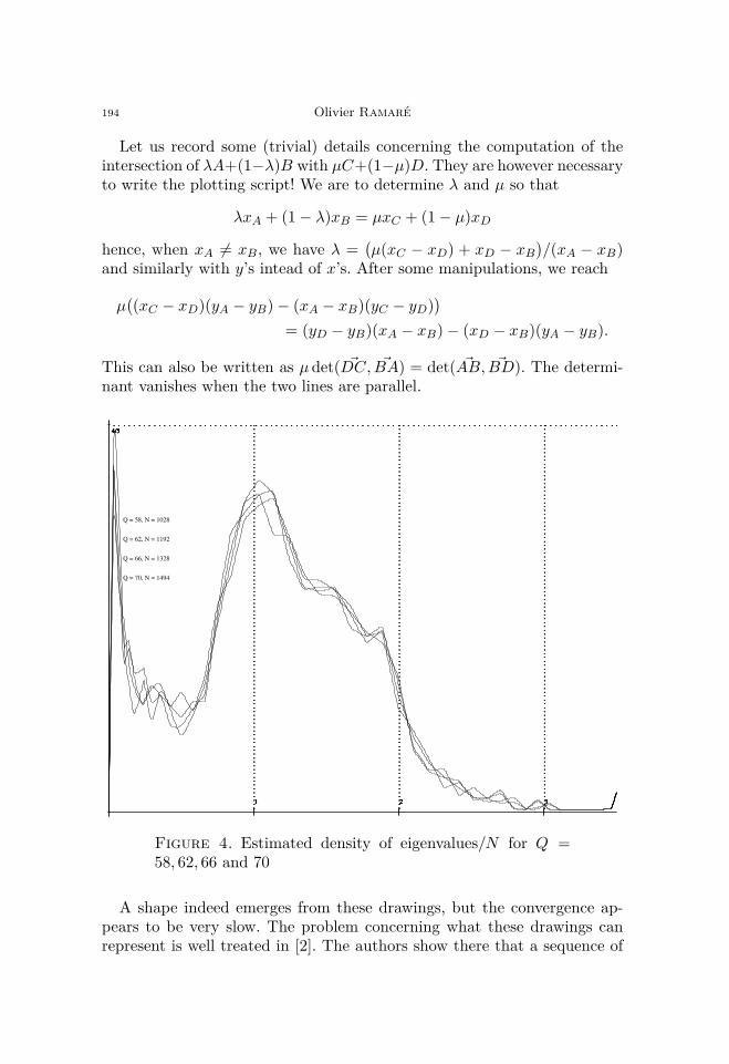
Figure 4. Estimated density of eigenvalues/N for Q =58, 62, 66 and 70
A shape indeed emerges from these drawings, but the convergence ap-pears to be very slow. The problem concerning what these drawings canrepresent is well treated in [2]. The authors show there that a sequence of
Eigenvalues in the large sieve inequality, II 195
measures, say (µn)n≥1, each of them satisfying
∀k ≤ n,∫tkdµn =
∫tkdµ,
converges weakly towards µ. However, they also exhibit a sequence of func-tions (and a measure µ) such that
∀k ≤ n,∫tkfn(t)dµ =
∫tkf(t)dµ
while (fn)n≥1 does not converge towards f . This is most probably a patho-logical case, but it is worth mentionning it, especially in the light of sec-tion 3.
References[1] E. Bombieri, Le grand crible dans la théorie analytique des nombres. Astérisque 18 (1987).[2] J.M. Borwein and A.S. Lewis, On the convergence of moment problems. Trans. Amer.
Math. Soc. 325(1) (1991), 249–271.[3] G. Greaves, An algorithm for the Hausdorff moment problem. Numerische Mathematik
39(2) (1982), 231–238.[4] F. Hausdorff, Summationsmethoden und Momentfolgen. I. Math. Z. 9 (1921), 74–109.[5] F. Hausdorff, Summationsmethoden und Momentfolgen. II. Math. Z. 9 (1921), 280–299.[6] F. Hausdorff,Momentenprobleme für ein endliches Intervall. Math. Z. 16 (1923), 220–248.[7] H.L. Montgomery, Topics in Multiplicative Number Theory. Lecture Notes in Mathematics
(Berlin) 227. Springer–Verlag, Berlin–New York, 1971.[8] I.J. Schoenberg, R. Askey and A. Sharma, Hausdorff’s moment problem and expansions
in Legendre polynomials. J. Math. Anal. Appl. 86 (1982), 237–245.[9] O. Ramaré, Eigenvalues in the large sieve inequality. Funct. Approximatio, Comment.
Math. 37 (2007), 7–35.[10] A. Selberg, Collected papers. Springer–Verlag, Berlin, 1991.[11] J. Szabados, On the convergence and saturation problem of the Jackson polynomials. Acta
Math. Acad. Sci. Hungar. 24 (1973), 399–406.
Olivier RamaréLaboratoire CNRS Paul Painlevé,Université Lille 1,59 655 Villeneuve d’Ascq cedex, FranceE-mail: [email protected]


