Embed Size (px)
Citation preview
HAL Id: hal-03091852https://hal.archives-ouvertes.fr/hal-03091852
Submitted on 31 Dec 2020
HAL is a multi-disciplinary open accessarchive for the deposit and dissemination of sci-entific research documents, whether they are pub-lished or not. The documents may come fromteaching and research institutions in France orabroad, or from public or private research centers.
L’archive ouverte pluridisciplinaire HAL, estdestinée au dépôt et à la diffusion de documentsscientifiques de niveau recherche, publiés ou non,émanant des établissements d’enseignement et derecherche français ou étrangers, des laboratoirespublics ou privés.
Electromagnetic waves in photonic crystals: laws ofdispersion, causality and analytical properties
Boris Gralak, Sébastien Guenneau, Maxence Cassier, Guillaume Demésy
To cite this version:Boris Gralak, Sébastien Guenneau, Maxence Cassier, Guillaume Demésy. Electromagnetic waves inphotonic crystals: laws of dispersion, causality and analytical properties. Compendium on Electro-magnetic Analysis From Electrostatics to Photonics: Fundamentals and Applications for Physicistsand Engineers Volume 4: Optics and Photonics I, 2020, 10.1142/10987-vol4. hal-03091852
Electromagnetic waves in photonic crystals: laws of dispersion,
causality and analytical properties
Boris Gralak†, Maxence Cassier, Guillaume Demesy and Sebastien Guenneau
Aix Marseille Univ, CNRS, Centrale MarseilleInstitut Fresnel, Marseille, France
Abstract
Photonic crystals are periodic structures which prevent light propagation alongone or more directions in certain frequency intervals. Their band spectrum is usuallyanalyzed using Floquet-Bloch decomposition. This spectrum is located on the realaxis, and it enters the complex plane when absorption and dispersion is consideredin the dielectric permittivity of material constituents. Here, we review fundamentaldefinition and properties of dispersion law and group velocity in photonic crystals andwe illustrate them with numerical examples.
1 Introduction
Photonic crystals are periodic electromagnetic structures that have been originally intro-duced by Eli Yablonovith [1] and Sajeev John [2] in order to inhibit the spontaneous emission[3, 1] and obtain strong localization of photons[2]. The original idea, based on an analogywith solid states Physics [4], was to use the periodic modulation in two or three dimensionsof a lossless dielectric permittivity to open photonic bandgaps, i.e. ranges of frequencieswhere for which the electromagnetic radiation cannot propagate [5]. If an excited atom isembedded in such a periodic medium and if its energy level corresponds to a frequency ofthe bandgap, then photons cannot be radiated. Therefore photons can be strongly localized[2] and the spontaneous emission can be inhibited [3].
Hence, an important challenge of photonic crystals topic was to obtain in three-dimensionsat optical wavelengths a full photonic bandgap (i.e. light is disallowed to propagate along alldirections) sufficiently robust to the fabrication imperfections. The most promising struc-tures have probably been the photonic crystals produced using colloidal suspensions [6, 7],layer-by-layer semiconductor industry technique [8, 9, 10, 11] and inverse opal synthesis[12, 13]. Nevertheless, the fabrication of such three-dimensional structures remains difficultto proceed, notably in comparison with the fabrication of two-dimensional photonic crystalsfor which the semiconductor techniques can be directly transposed to etch membranes orslabs on substrate [14].
The ability of two-dimensional photonic crystals to forbid the propagation of the elec-tromagnetic field has been exploited to guide light in microstructured optical fibres [15, 16,17, 18, 19, 20] and planar structures in integrated optics [21]. In photonic crystal fibers thephotonic bandgap allows the guiding of light in air or vacuum, thus enabling to enhance thepower of the guided light. In integrated optics, the objective was to obtain optical circuitswith both reduced dimensions and a reduction of the radiation losses [22]. Furthermore,the two-dimensional photonic bandgap has been used to design cavities with high qualityfactor [23, 24], with applications to the enhancement of the efficiency of light sources andsensors. In that case, the enhancement of the emission of photons and the electromagneticlocal density of states is based on the existence of bandgaps, i.e. the absence of photonicmodes for certain frequency ranges in photonic crystals.
The photonic bands themselves can be also exploited to obtain a fine control of theemission and propagation of electromagnetic waves. In addition to its enhancement, theemission of electromagnetic waves can be channelled around specific directions as soon as
1
arX
iv:1
807.
0165
8v1
[ph
ysic
s.op
tics]
4 J
ul 2
018
the photonic bands are restricted to the corresponding ranges of wavevectors [25], withapplications to directive antennas [26]. The propagation of electromagnetic waves is governedby the photonic bands providing the dispersion law and the group velocity [27, 28]. Therichness of the dispersion law can lead to an enhanced dispersive effect or, conversely, to aself guiding effect [29], and to exotic refraction properties like ultra-refraction and negativerefraction [30]. In particular, negative refraction from photonic crystals [31, 32, 33] can beconsidered as an alternative to negative index from metamaterials [34, 35, 36] since it is notspoiled by absorption.
All the aforementioned effects and applications are governed by the photonic bands andgaps which are totally determined by the relationship between the frequency ω and thewavevector k, namely the dispersion law. This chapter will be devoted to this relationshipincluding the last developments with dispersion and absorption. After the presentation ofMaxwell’s equations in photonic crystals in section 2, the Floquet-Bloch decomposition isintroduced in section 3. It is shown that this Floquet-Bloch decomposition is a unitarytransform which is specially adapted to partial differential equations with periodic coef-ficients since it commutes with multiplicative operator by periodic functions. Then, thedispersion law ω(k) is introduced in section 4 and it is shown that the group velocity ∂kω(k)governs the propagation of the electromagnetic field. In section 5, numerical calculations ofthe dispersion law are presented in the case of two-dimensional photonic crystals. In addi-tion, the effect of the effective anisotropy on the propagation of the electromagnetic field isnumerically illustrated in two-dimensional photonic crystals. In section 6 the dispersion lawis extended to dispersive and absorptive photonic crystals and numerical calculation of thecomplex spectrum of Bloch resonances are provided for two-dimensional photonic crystalsmade of a Drude metal. Finally, the analytic nature of the dispersion law is discussed insection 7.
2 Maxwell’s equations in photonic crystals
In this chapter, different bases are used: (e1, e2, e3) is an orthonormal basis; (a1, a2, a3)is the basis defining the lattice associated with the photonic crystal, hence it need not beorthonormal; and (K 1,K 2,K 3) is the basis defining the reciprocal lattice. Every vector xin R3 (respectively in C3) of the physical space is described by three components x1, x2 andx3 in R (respectively in C).
We start with macroscopic Maxwell’s equations in linear, dispersion-free dielectric media:
∂x ×E(x, t) = −µ0∂tH (x, t) ,
∂x ×H (x, t) = ε(x)∂tE(x, t) + J (x, t) ,(1)
where E(x, t) and H (x, t) are the electric and magnetic fields, J (x, t) is the current sourcedensity, ∂x× is the curl operator, µ0 is the vacuum permeability and ε(x) is the dielectricpermittivity. The dielectric permittivity ε(x) in photonic crystals is generally consideredas a frequency-independent function taking real and positive values greater than the one ofthe vacuum permittivity ε0. Indeed, such functions can describe lossless dielectric materialswhich are good candidates to obtain bandgap in photonic crystals [37], while the presenceof absorption implies the absence of bandgaps [38]. In this chapter, the case of dispersiveand absorptive permittivity is addressed in the section 6. In the other sections, one assumesthat the photonic crystal is neither dispersive nor dissipative.
Let a1, a2, and a3 be the linearly-independent and non-vanishing vectors of R3 definingthe unit cell V of the periodic photonic crystal:
V =x = x1a1 + x2a2 + x3a3
∣∣x1, x2, x3 ∈ [0, 1]. (2)
Then, the lattice L associated with the photonic crystal is
L =a = p1a1 + p2a2 + p3a3
∣∣ p1, p2, p3 ∈ Z
(3)
2
and the permittivity ε(x) determining the geometry of the crystal is invariant under the setof translations by the vectors of the lattice:
ε(x + a) = ε(x) , x ∈ R3 , a ∈ L . (4)
The basis (K 1,K 2,K 3) of the reciprocal lattice is defined such that K i · aj = 2πδij withδij the Kronecker symbol (δij = 1 if i = j and δij = 0 otherwise):
K 1 =2π
Aa2 × a3 , K 2 =
2π
Aa3 × a1 , K 3 =
2π
Aa1 × a2 , (5)
where A = | (a1×a2) ·a3 | 6= 0 is the volume of the unit cell V . Finally, the reciprocal latticeis defined by
L∗ =K = p1K 1 + p2K 2 + p3K 3
∣∣ p1, p2, p3 ∈ Z
(6)
and the unit cell B of this reciprocal lattice, or the first Brillouin zone, is given by
B =k = k1K 1 + k2K 2 + k3K 3
∣∣ k1, k2, k3 ∈ [−1/2, 1/2]. (7)
The following purely electromagnetic quantity, corresponding to the electromagnetic en-ergy if the field is in vacuum, is assumed to be finite for all time t:
E(t) =1
2
∫R3
dx[ε0E(x, t)2 + µ0H (x, t)2
]<∞ . (8)
This assumption implies that the electromagnetic fields E(x, t) and H (x, t) are square inte-
grable functions of the position x with well-defined Fourier transforms E(k, t) and H(k, t).
3 The Floquet-Bloch decomposition
The Floquet-Bloch decomposition is a unitary transform adapted to partial derivative equa-tions with periodic coefficients [39, 40]. This decomposition exploits the invariance of theequations under the group of symmetries formed by the set of translations by the vectors ain the lattice L (3). In this chapter, it is shown that the Maxwell’s equations (1) with peri-odic permittivity ε(x) are equivalent to a family of similar equations indexed by the Blochwavevector k and restricted to the unit cell V . Also, the electromagnetic fields E(x, t) andH (x, t) can be uniquely defined as the superposition of Bloch waves indexed by the Blochwavevector k spanning the Brillouin zone B. The arguments supporting these results, basedon the Fourier transform and Fourier series are briefly presented and then are concluded bya summary on the Floquet-Bloch decomposition.
From the Fourier analysis to the Floquet-Bloch decomposition. The Fourier trans-forms E(k, t) and H(k, t) can be related to the fields E(x, t) and H (x, t) with the followingintegral expressions: for F = E ,H
F (k, t) =
∫R3
dx exp[−ik · x]F (x, t) , (9)
and, conversely,
F (x, t) =1
(2π)3
∫R3
dk exp[ik · x] F (k, t) . (10)
This last expression can be decomposed using the reciprocal lattice:
F (x, t) =1
(2π)3
∫B
dk∑
K∈L∗
exp[i(k + K ) · x] F (k + K , t) . (11)
Let F#(x, k, t) denote the series under the integral:
F#(x, k, t) =1
(2π)3
∑K∈L∗
exp[i(k + K ) · x] F (k + K , t) . (12)
3
This function appears to be periodic of k, i.e. invariant under translations of vectors K inthe reciprocal lattice L∗. Hence, it can be expanded as the Fourier series
F#(x, k, t) =∑a∈L
exp[−ik · a]A
(2π)3
∫B
dk′ exp[ik′ · a]F#(x, k′, t) . (13)
where it has been used that (2π)3/A = |(K 1×K 2) ·K 3| is the volume of the first Brillouinzone B. Replacing F#(x, k′, t) by its series expression (12), the coefficients of the Fourierseries become (up to the factor A/(2π)3)∫
B
dk′ exp[ik′ · a]F#(x, k′, t)
=
∫B
dk′ exp[ik′ · a]1
(2π)3
∑K∈L∗
exp[i(k′ + K ) · x] F (k′ + K , t)
=
∫B
dk′1
(2π)3
∑K∈L∗
exp[i(k′ + K ) · (x + a)] F (k′ + K , t) ,
(14)
where we used that exp[iK · a] = 1. From (11), the coefficients in (13)–(14) are∫B
dk′ exp[ik′ · a]F#(x, k′, t) = F (x + a, t) . (15)
Hence, combining (11), (12), (13) and (15), we deduce that the function F (x, t) can bewritten as the superposition over the the first Brillouin zone
F (x, t) =
∫B
dkF#(x, k, t) , (16)
with components
F#(x, k, t) =A
(2π)3
∑a∈L
exp[−ik · a]F (x + a, t) . (17)
The linear transformation (17) that defines F#(x, k, t) in term of F (x, t) is usually referredin the literature[40] as the Floquet-Bloch transform of the function F (x, t), whereas theequation (16) gives the expression of the inverse of this transform. In addition, a Parsevalidentity between the norms of F (x, t) and F#(x, k, t), in the sense of square integrablefunctions, can be derived. Starting with the square of the norm of F (x, t), the integral overthe variable x is decomposed according to the L-lattice:∫
R3
dx∣∣F (x, t)
∣∣2 =
∫V
dx∑a∈L
∣∣F (x + a, t)∣∣2 . (18)
From (17), the function F#(x, k, t) is periodic of k and the coefficients of its series expansionare F (x + a, t). Hence, the square of the norm of F#(x, k, t) is
A
(2π)3
∫B
dk∣∣F#(x, k, t)
∣∣2 =∑a∈L
∣∣F (x + a, t)∣∣2 , (19)
and the identity (18) becomes∫R3
dx∣∣F (x, t)
∣∣2 =A
(2π)3
∫V
dx
∫B
dk∣∣F#(x, k, t)
∣∣2 . (20)
Notice that the integrals and the series have been manipulated formally without particularcautions. Rigorously, it is necessary to first consider fields decreasing “rapidly” (e.g. in theSchwartz space[41]) and then to extend the results to all finite energy (square integrable)fields using a density argument.
4
Summary. The electromagnetic fields F (x, t) with finite energy can be decomposed as thesuperposition (16), over the first Brillouin zone B, of the Bloch waves F#(x, k, t) given by theequation (17). The Bloch waves F#(x, k, t), defined for all Bloch wavevector k, represent theFloquet-Bloch transform of F (x, t). From (20), the Floquet-Bloch transform is an isometryand the decomposition (16) is unique. The Floquet-Bloch transform F#(x, k, t) is a L∗-periodic function with respect to the Bloch wavevector k while, with respect to the spacevariable x, it satisfies the Bloch requirement
F#(x + a, k, t) = exp[ik · a]F#(x, k, t) , a ∈ L . (21)
It is important to notice that the Floquet-Bloch transform of ε(x)E(x, t) is (17)[εE]#
(x, k, t) =A
(2π)3
∑a∈L
exp[−ik · a] ε(x + a)E(x + a, t)
=A
(2π)3
∑a∈L
exp[−ik · a] ε(x)E(x + a, t)
= ε(x)E#(x, k, t) .
(22)
In other words, the Floquet-Bloch transform commutes with the multiplicative operator bythe periodic function ε(x). Thus the Floquet-Bloch transform appears to be particularlyadapted to partial differential equations with periodic coefficients. The application of theFloquet-Bloch transform to the Maxwell’s equations (1) leads to the following family ofindependent equations indexed by the Bloch wavevector k spanning the first Brillouin zoneB:
∂x ×E#(x, k, t) = −µ0∂tH#(x, k, t) ,
∂x ×H#(x, k, t) = ε(x)∂tE#(x, k, t) + J#(x, k, t) .(23)
Each equation indexed by k can be solved separately for fields E#(x, k, t) and H#(x, k, t)that are square integrable with respect to x on the unit cell V . Finally, the solutions E(x, t)and H (x, t) of the initial Maxwell’s equations are retrieved performing the superpositionover the first Brillouin zone:
E(x, t) =
∫B
dkE#(x, k, t) , H (x, t) =
∫B
dkH#(x, k, t) . (24)
The Floquet-Bloch transform appears as the tool to decompose periodic equations into aset of equations restricted to the unit cell V . This transform leads also to the introductionof the Bloch wavevector k, which is the fundamental physical conserved quantity associatedwith the group of symmetries formed by the set of translations of vector a in L.
4 The dispersion law
The Maxwell’s equations (1) are invariant under any translation with respect to the time t.That suggests to decompose the equations with respect to the time and to consider them inthe time-harmonic regime.
We start with Maxwell’s equations (23) after the Floquet-Bloch decomposition and withthe current source J#(x, k, t) set to zero. Assuming that a Fourier decomposition withrespect to the time can be applied to these equations1, the following set of equations isobtained:
∂x ×E#(x, k, ω) = iωµ0H#(x, k, ω) ,
∂x ×H#(x, k, ω) = −iωε(x)E#(x, k, ω) ,(25)
1It is stressed that the Fourier decomposition with respect to the time of equations (23) [or (1)] is notstraightforward when the electromagnetic energy is conserved, and it has to be considered in the sense ofdistributions. An alternative way is to perform a Laplace transform[42] to the equations for a frequency ωwith a positive imaginary part [43]. Then, the limit Im(ω) ↓ 0 can be considered to define the time-harmonicMaxwell’s equations (or the Helmholtz operator).
5
where E#(x, k, ω) and H#(x, k, ω) are the time-harmonic electric and magnetic fields oscil-lating at the frequency ω, with the Bloch boundary condition (21). This set of equations(25) can be expressed as the eigenvalue problem
M(x, k)F#(x, k, ω) = ω F#(x, k, ω) , (26)
where
F#(x, k, ω) =
[E#(x, k, ω)H#(x, k, ω)
]exp[−ik · x] , (27)
is a square integrable periodic function of x on the unit cell V and
M(x, k) =
[0 iε−1(x)(∂x + ik)×−iµ−10 (∂x + ik)× 0
], (28)
is an operator depending on the Bloch wavevector k. The solutions of time-harmonicMaxwell equations (25) without sources are the Bloch modes of the photonic crystal.These modes are proportional to the eigenvectors F#(x, k, ω) of the operator M(x, k) actingon the square integrable periodic functions of x on the unit cell V . The oscillating frequen-cies ω of the Bloch modes are the eigenvalues of the operator M(x, k), hence they dependon the wavevector k. This relationship ω(k) defines the dispersion law.
The dispersion law ω(k) and the Bloch modes play a fundamental role. Indeed, thesolutions of Maxwell’s equations in photonic crystals can be expressed as a superposition(24) of Bloch modes. As to the dispersion law ω(k), it provides the relationship between thetwo physical invariant quantities ω and k resulting from the temporal and spatial symmetries.It governs the propagation of the electromagnetic field through the group velocity [27]
vg = [∂kω](k) . (29)
This property can be justified using the following arguments. Let X (t) be the center of theelectric field intensity:
X (t) =
∫R3
dx xE(x, t)2∫R3
dxE(x, t)2, (30)
where E(x, t) = E(x, t) since the time dependent field is real. Using the unitary property ofthe Floquet-Bloch transform, this vector becomes
X (t) =
∫V
dx
∫B
dk [xE ]#(x, k, t) ·E#(x, k, t)∫V
dx
∫B
dk∣∣E#(x, k, t)
∣∣2 (31)
Next, the Floquet-Bloch transform of xE(x, t) is derived from the expression (17):
[xE ]#(x, k, t) =∑a∈L
exp[−ik · a] (x + a)E(x + a, t) = (x + i∂k)E#(x, k, t) . (32)
Then, it is assumed that each Floquet-Bloch component E#(x, k, t) is made of a single time-harmonic Bloch mode2 oscillating at the frequency ω(k): E#(x, k, t) = E#(x, k) exp[−iω(k)t].Hence the expression above becomes
[xE ]#(x, k, t) =
[x + i∂k]E#(x, k) + [∂kω](k) tE#(x, k)
exp[−iω(k)t] , (33)
and the vector X (t) can be written
X (t) = X 0 + V t , (34)
2If the components E#(x, k, t) contain several Bloch modes, then a finite sum over the correspondingbands is obtained: note that each band has a different group velocity.
6
where the vectors X 0 and V are time-independent:
X 0 =
∫V
dx
∫B
dk [x + i∂k]E#(x, k) · E#(x, k)∫V
dx
∫B
dk∣∣E#(x, k)
∣∣2 , (35)
and
V =
∫V
dx
∫B
dk [∂kω](k)∣∣E#(x, k)
∣∣2∫V
dx
∫B
dk∣∣E#(x, k)
∣∣2 . (36)
Thus the vector V appears as the velocity of the field intensity center. Its expressionas the average of the group velocity shows that the latter governs the propagation of theelectromagnetic field. Similar averaged expressions can be established for the center of themagnetic field intensity or the center of the electromagnetic field energy density. In the nextsection, this property of the group velocity is exploited to show the effect of the photoniccrystal on the propagation of the electromagnetic field.
5 Computation of the dispersion law and applications
The dispersion law in photonic crystals has been investigated intensively with differentnumerical methods. Since the eigenvalue problem (26) is defined from the periodic operatorM(x, k) acting on the Hilbert space of square integrable periodic functions of x, the mostwidely used numerical method was based on the expansion of the equations into the discreteFourier (or plane-waves) basis [44, 45, 46]. This expansion was used to predict photonicbandgap edges [47], the effect of several structural imperfections on such edges [48], thedecay rate for single photon emission in infinite structures [49] and reflectivity and theinhibition of spontaneous emission for finite-thickness structures [50]. An efficient softwarebased on this method, MPB3 for MIT Photonic Bands, has been elaborated by StevenJohnson and John Joannopoulos [51].
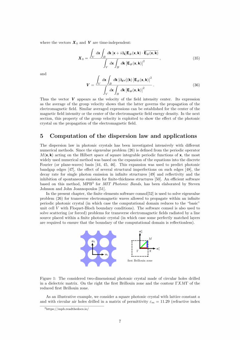
In the present chapter, the finite elements software comsol[52] is used to solve eigenvalueproblem (26) for transverse electromagnetic waves allowed to propagate within an infiniteperiodic photonic crystal (in which case the computational domain reduces to the “basic”unit cell V with Floquet-Bloch boundary conditions). The software comsol is also used tosolve scattering (or forced) problems for transverse electromagnetic fields radiated by a linesource placed within a finite photonic crystal (in which case some perfectly matched layersare required to ensure that the boundary of the computational domain is reflectionless).
a1
a2
a∗1
a∗2
Γ X
M
first Brillouin zone
Figure 1: The considered two-dimensional photonic crystal made of circular holes drilledin a dielectric matrix. On the right the first Brillouin zone and the contour ΓXMΓ of thereduced first Brillouin zone.
As an illustrative example, we consider a square photonic crystal with lattice constant aand with circular air holes drilled in a matrix of permittivity εm = 11.29 (refractive index
3https://mpb.readthedocs.io/
7
n = 3.36). This permittivity value corresponds to the effective index of s-polarized mode ina planar waveguide made of InGaAsP [53]. The radius of the circular holes is set to 0.455a,and this corresponds to the air filling ratio of 0.65. The unit cell of the crystal is definedby the two vectors a1 = a e1 and a2 = a e2, and the first Brillouin zone by the vectorsK 1 = (2π/a) e1 and K 2 = (2π/a) e2 (see Fig. 1). According to the symmetries of the unitcell, the dispersion law is represented on the path ΓXMΓ in the first Brillouin zone withΓ = (0, 0), X = (1/2, 0) and M = (1/2, 1/2) in the basis (K 1,K 2). We compute the banddiagrams associated with transverse electromagnetic waves propagating in the plane (a1, a2).In this cylindrical case, one can split the two-dimensional spectral problem (25) into the twoscalar situations identified by the s- and p-polarizations (also referenced by, respectively, theTM and TE cases [37]). Denoting by E# ≡ E#,3 and H# ≡ H#,3 the components of E#
and H# along the axis e3 of invariance, we look for pairs of eigenfrequencies and associatedeigenfields, (ω,E#) for s-polarization and (ω,H#) for p-polarization, solutions of
−∂x · ∂xE#(x, k, ω) = ω2µ0 ε(x)E#(x, k, ω) ,
−∂x · ε−1(x) ∂xH#(x, k, ω) = ω2µ0H#(x, k, ω) ,(37)
and such that E# and H# satisfy the Floquet-Bloch conditions (21) on the opposite edgesof the periodic unit cell V . Notice that, in the present two-dimensional case, the variablesx and k are the two-components vectors (x1, x2) and (k1, k2). This problem is discretizedusing finite elements, and it is implemented with comsol[52].
s-polarization p-polarization
norm
alize
dfr
equ
ency
ωa/(2πc)
0
0.1
0.2
0.3
0.4
0.5
0.6
0.7
0.8
0.9
1
ΓX MΓ
a cω /(2π )
norm
alize
dfr
equ
ency
ωa/(2πc)
0
0.1
0.2
0.3
0.4
0.5
0.6
0.7
0.8
0.9
1
X ΓMΓ
a cω /(2π )
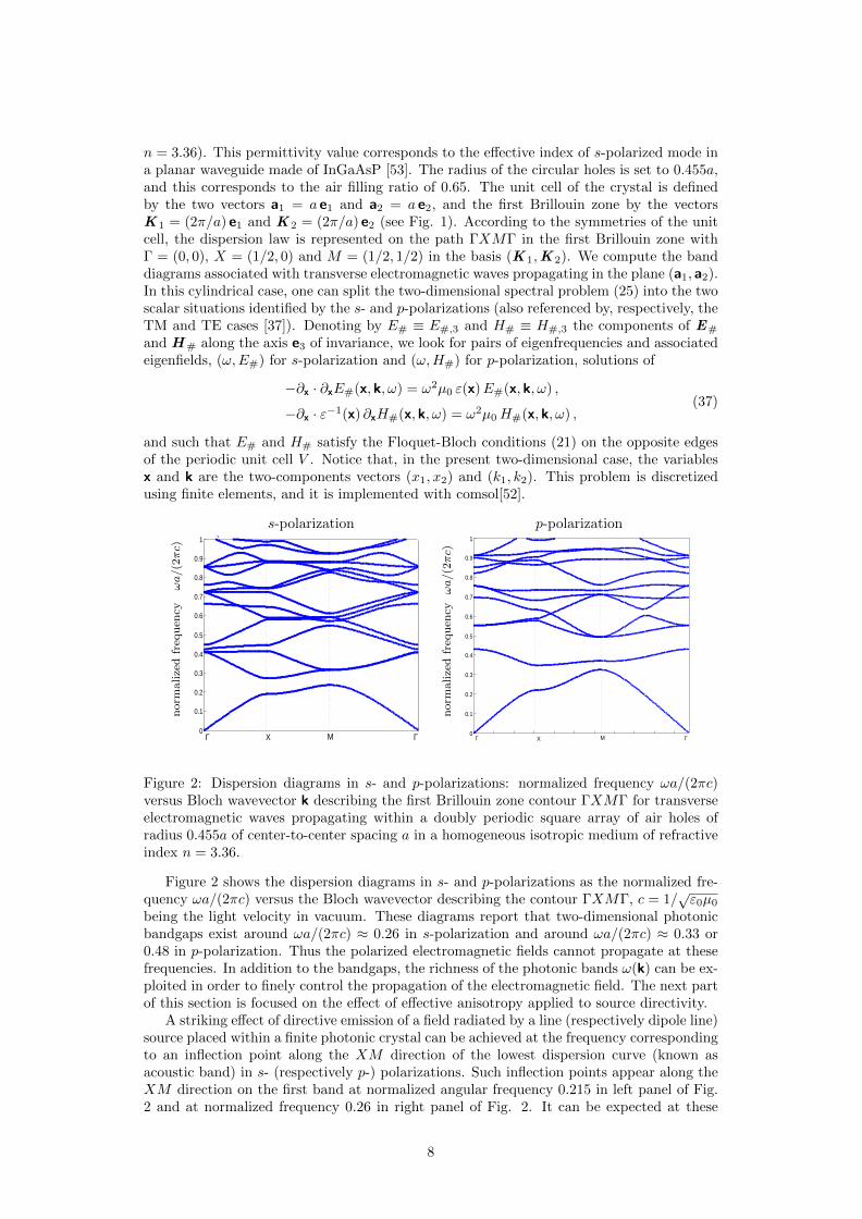
Figure 2: Dispersion diagrams in s- and p-polarizations: normalized frequency ωa/(2πc)versus Bloch wavevector k describing the first Brillouin zone contour ΓXMΓ for transverseelectromagnetic waves propagating within a doubly periodic square array of air holes ofradius 0.455a of center-to-center spacing a in a homogeneous isotropic medium of refractiveindex n = 3.36.
Figure 2 shows the dispersion diagrams in s- and p-polarizations as the normalized fre-quency ωa/(2πc) versus the Bloch wavevector describing the contour ΓXMΓ, c = 1/
√ε0µ0
being the light velocity in vacuum. These diagrams report that two-dimensional photonicbandgaps exist around ωa/(2πc) ≈ 0.26 in s-polarization and around ωa/(2πc) ≈ 0.33 or0.48 in p-polarization. Thus the polarized electromagnetic fields cannot propagate at thesefrequencies. In addition to the bandgaps, the richness of the photonic bands ω(k) can be ex-ploited in order to finely control the propagation of the electromagnetic field. The next partof this section is focused on the effect of effective anisotropy applied to source directivity.
A striking effect of directive emission of a field radiated by a line (respectively dipole line)source placed within a finite photonic crystal can be achieved at the frequency correspondingto an inflection point along the XM direction of the lowest dispersion curve (known asacoustic band) in s- (respectively p-) polarizations. Such inflection points appear along theXM direction on the first band at normalized angular frequency 0.215 in left panel of Fig.2 and at normalized frequency 0.26 in right panel of Fig. 2. It can be expected at these
8
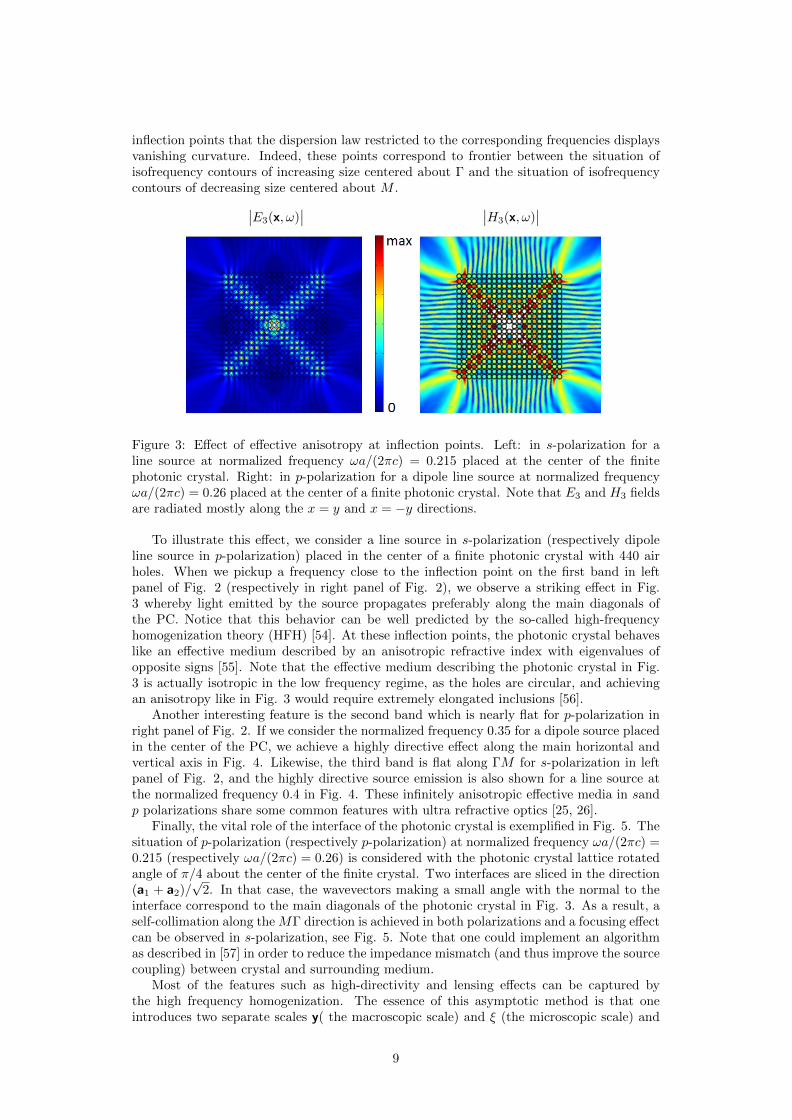
inflection points that the dispersion law restricted to the corresponding frequencies displaysvanishing curvature. Indeed, these points correspond to frontier between the situation ofisofrequency contours of increasing size centered about Γ and the situation of isofrequencycontours of decreasing size centered about M .∣∣E3(x, ω)
∣∣ ∣∣H3(x, ω)∣∣
Figure 3: Effect of effective anisotropy at inflection points. Left: in s-polarization for aline source at normalized frequency ωa/(2πc) = 0.215 placed at the center of the finitephotonic crystal. Right: in p-polarization for a dipole line source at normalized frequencyωa/(2πc) = 0.26 placed at the center of a finite photonic crystal. Note that E3 and H3 fieldsare radiated mostly along the x = y and x = −y directions.
To illustrate this effect, we consider a line source in s-polarization (respectively dipoleline source in p-polarization) placed in the center of a finite photonic crystal with 440 airholes. When we pickup a frequency close to the inflection point on the first band in leftpanel of Fig. 2 (respectively in right panel of Fig. 2), we observe a striking effect in Fig.3 whereby light emitted by the source propagates preferably along the main diagonals ofthe PC. Notice that this behavior can be well predicted by the so-called high-frequencyhomogenization theory (HFH) [54]. At these inflection points, the photonic crystal behaveslike an effective medium described by an anisotropic refractive index with eigenvalues ofopposite signs [55]. Note that the effective medium describing the photonic crystal in Fig.3 is actually isotropic in the low frequency regime, as the holes are circular, and achievingan anisotropy like in Fig. 3 would require extremely elongated inclusions [56].
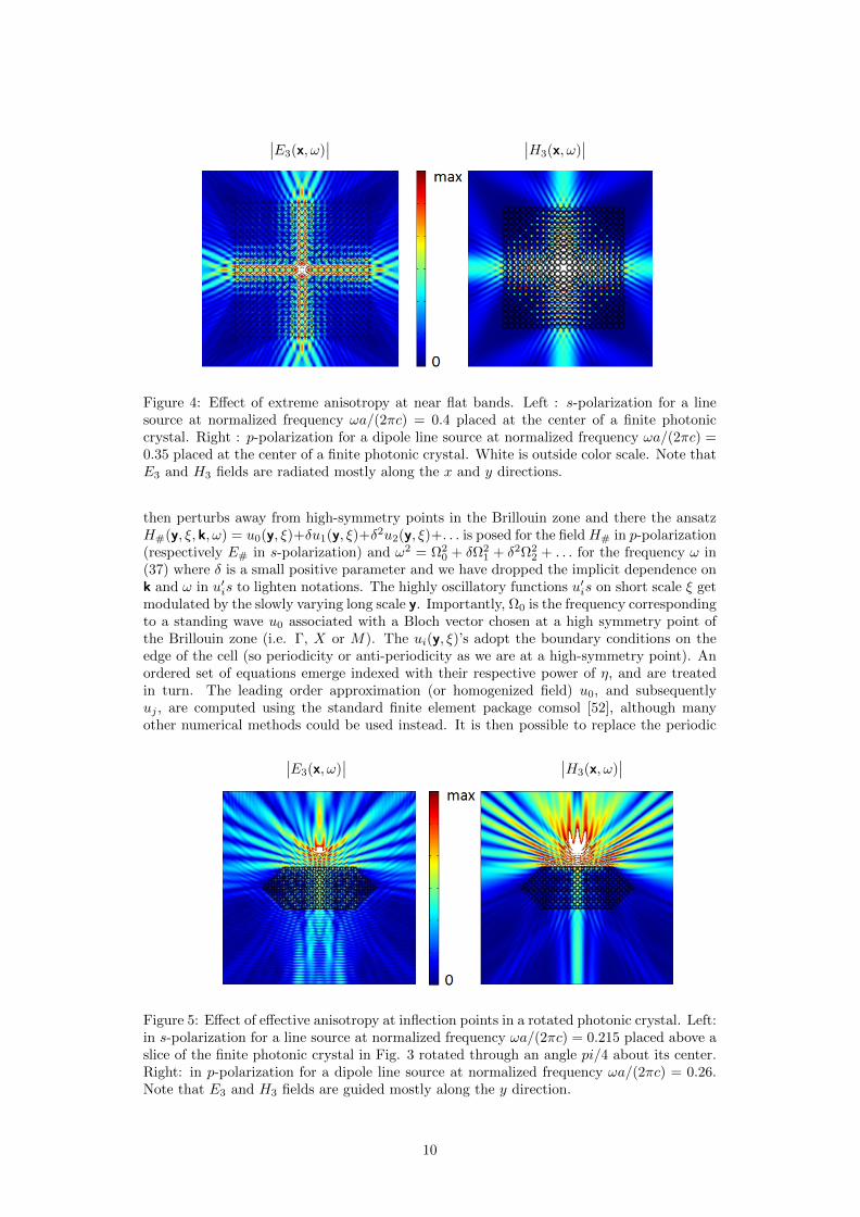
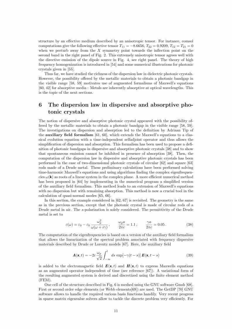
Another interesting feature is the second band which is nearly flat for p-polarization inright panel of Fig. 2. If we consider the normalized frequency 0.35 for a dipole source placedin the center of the PC, we achieve a highly directive effect along the main horizontal andvertical axis in Fig. 4. Likewise, the third band is flat along ΓM for s-polarization in leftpanel of Fig. 2, and the highly directive source emission is also shown for a line source atthe normalized frequency 0.4 in Fig. 4. These infinitely anisotropic effective media in sandp polarizations share some common features with ultra refractive optics [25, 26].
Finally, the vital role of the interface of the photonic crystal is exemplified in Fig. 5. Thesituation of p-polarization (respectively p-polarization) at normalized frequency ωa/(2πc) =0.215 (respectively ωa/(2πc) = 0.26) is considered with the photonic crystal lattice rotatedangle of π/4 about the center of the finite crystal. Two interfaces are sliced in the direction(a1 + a2)/
√2. In that case, the wavevectors making a small angle with the normal to the
interface correspond to the main diagonals of the photonic crystal in Fig. 3. As a result, aself-collimation along the MΓ direction is achieved in both polarizations and a focusing effectcan be observed in s-polarization, see Fig. 5. Note that one could implement an algorithmas described in [57] in order to reduce the impedance mismatch (and thus improve the sourcecoupling) between crystal and surrounding medium.
Most of the features such as high-directivity and lensing effects can be captured bythe high frequency homogenization. The essence of this asymptotic method is that oneintroduces two separate scales y( the macroscopic scale) and ξ (the microscopic scale) and
9
∣∣E3(x, ω)∣∣ ∣∣H3(x, ω)
∣∣
Figure 4: Effect of extreme anisotropy at near flat bands. Left : s-polarization for a linesource at normalized frequency ωa/(2πc) = 0.4 placed at the center of a finite photoniccrystal. Right : p-polarization for a dipole line source at normalized frequency ωa/(2πc) =0.35 placed at the center of a finite photonic crystal. White is outside color scale. Note thatE3 and H3 fields are radiated mostly along the x and y directions.
then perturbs away from high-symmetry points in the Brillouin zone and there the ansatzH#(y, ξ, k, ω) = u0(y, ξ)+δu1(y, ξ)+δ2u2(y, ξ)+. . . is posed for the field H# in p-polarization(respectively E# in s-polarization) and ω2 = Ω2
0 + δΩ21 + δ2Ω2
2 + . . . for the frequency ω in(37) where δ is a small positive parameter and we have dropped the implicit dependence onk and ω in u′is to lighten notations. The highly oscillatory functions u′is on short scale ξ getmodulated by the slowly varying long scale y. Importantly, Ω0 is the frequency correspondingto a standing wave u0 associated with a Bloch vector chosen at a high symmetry point ofthe Brillouin zone (i.e. Γ, X or M). The ui(y, ξ)’s adopt the boundary conditions on theedge of the cell (so periodicity or anti-periodicity as we are at a high-symmetry point). Anordered set of equations emerge indexed with their respective power of η, and are treatedin turn. The leading order approximation (or homogenized field) u0, and subsequentlyuj , are computed using the standard finite element package comsol [52], although manyother numerical methods could be used instead. It is then possible to replace the periodic
∣∣E3(x, ω)∣∣ ∣∣H3(x, ω)
∣∣
Figure 5: Effect of effective anisotropy at inflection points in a rotated photonic crystal. Left:in s-polarization for a line source at normalized frequency ωa/(2πc) = 0.215 placed above aslice of the finite photonic crystal in Fig. 3 rotated through an angle pi/4 about its center.Right: in p-polarization for a dipole line source at normalized frequency ωa/(2πc) = 0.26.Note that E3 and H3 fields are guided mostly along the y direction.
10
structure by an effective medium described by an anisotropic tensor. For instance, comsolcomputations give the following effective tensor T11 = −8.6656, T22 = 0.9209, T12 = T21 = 0when we perturb away from the X symmetry point towards the inflection point on thesecond band in the right panel of Fig. 2. This extremely anisotropic tensor agrees well withthe directive emission of the dipole source in Fig. 4, see right panel. The theory of highfrequency homogenization is introduced in [54] and some numerical illustrations for photoniccrystals given in [55].
Thus far, we have studied the richness of the dispersion law in dielectric photonic crystals.However, the possibility offered by the metallic materials to obtain a photonic bandgap inthe visible range [58, 59] motivates use of augmented formalisms of Maxwell’s equations[60, 42] for absorptive media : Metals are inherently absorptive at optical wavelengths. Thisis the topic of the next sections.
6 The dispersion law in dispersive and absorptive pho-tonic crystals
The notion of dispersive and absorptive photonic crystal appeared with the possibility of-fered by the metallic materials to obtain a photonic bandgap in the visible range [58, 59].The investigations on dispersion and absorption led to the definition by Adriaan Tip ofthe auxiliary field formalism [61, 60], which extends the Maxwell’s equations to a clas-sical evolution equation with a time-independent selfadjoint operator and thus allows thesimplification of dispersion and absorption. This formalism has been used to propose a defi-nition of photonic bandgaps in dispersive and absorptive photonic crystals [38] and to showthat spontaneous emission cannot be inhibited in presence of absorption [38]. Then, thecomputation of the dispersion law in dispersive and absorptive photonic crystals has beenperformed in the case of two-dimensional photonic crystals of circular [62] and square [63]rods made of a Drude metal. These preliminary calculations have been performed solvingtime-harmonic Maxwell’s equations and using algorithms finding the complex eigenfrequen-cies ω(k) as roots of a linear system in the complex plane. A more efficient numerical methodhas been proposed in [64] by implementing in the numerical program a simplified versionof the auxiliary field formalism. This method leads to an extension of Maxwell’s equationswith no dispersion but with remaining absorption. This method is now a crucial tool in thecalculation of quasi-normal modes [65, 66].
In this section, the example considered in [62, 67] is revisited. The geometry is the sameas in the previous section, except that the photonic crystal is made of circular rods of aDrude metal in air. The s-polarization is solely considered. The permittivity of the Drudemetal is set to
ε(ω) = ε0 − ε0ω2p
ω(ω + iγ),
ωpa
2πc= 1.1 ,
γa
2πc= 0.05 . (38)
The computation of the eigenfrequencies is based on a version of the auxiliary field formalismthat allows the linearization of the spectral problem associated with frequency dispersivematerials described by Drude or Lorentz models [67]. Here, the auxiliary field
A(x, t) = −2iωp√
2
∫ t
−∞ds exp[−γ(t− s)]E(x, t− s) (39)
is added to the electromagnetic field E(x, t) and H (x, t) to express Maxwells equationsas an augmented operator independent of time (see reference [67]). A variational form ofthe resulting augmented system is derived and discretized using the finite element method(FEM).
One cell of the structure described in Fig. 6 is meshed using the GNU software Gmsh [68].First or second order edge elements (or Webb elements[69]) are used. The GetDP [70] GNUsoftware allows to handle the required various basis functions handily. Very recent progressin sparse matrix eigenvalue solvers allow to tackle the discrete problem very efficiently. For
11
a1
a2
a∗1
a∗2
Γ X
M
first Brillouin zone
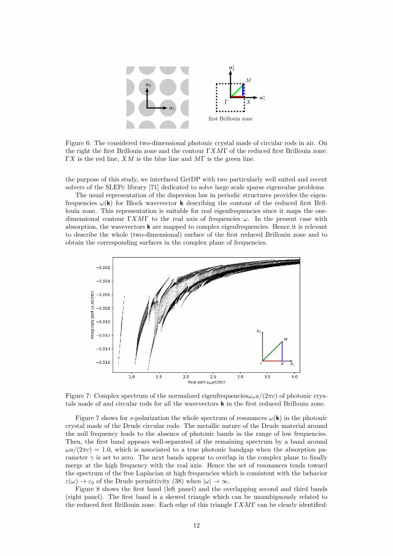
Figure 6: The considered two-dimensional photonic crystal made of circular rods in air. Onthe right the first Brillouin zone and the contour ΓXMΓ of the reduced first Brillouin zone:ΓX is the red line, XM is the blue line and MΓ is the green line.
the purpose of this study, we interfaced GetDP with two particularly well suited and recentsolvers of the SLEPc library [71] dedicated to solve large scale sparse eigenvalue problems.
The usual representation of the dispersion law in periodic structures provides the eigen-frequencies ω(k) for Bloch wavevector k describing the contour of the reduced first Bril-louin zone. This representation is suitable for real eigenfrequencies since it maps the one-dimensional contour ΓXMΓ to the real axis of frequencies ω. In the present case withabsorption, the wavevectors k are mapped to complex eigenfrequencies. Hence it is relevantto describe the whole (two-dimensional) surface of the first reduced Brillouin zone and toobtain the corresponding surfaces in the complex plane of frequencies.
Figure 7: Complex spectrum of the normalized eigenfrequenciesωna/(2πc) of photonic crys-tals made of and circular rods for all the wavevectors k in the first reduced Brillouin zone.
Figure 7 shows for s-polarization the whole spectrum of resonances ω(k) in the photoniccrystal made of the Drude circular rods. The metallic nature of the Drude material aroundthe null frequency leads to the absence of photonic bands in the range of low frequencies.Then, the first band appears well-separated of the remaining spectrum by a band aroundωa/(2πc) = 1.0, which is associated to a true photonic bandgap when the absorption pa-rameter γ is set to zero. The next bands appear to overlap in the complex plane to finallymerge at the high frequency with the real axis. Hence the set of resonances tends towardthe spectrum of the free Laplacian at high frequencies which is consistent with the behaviorε(ω)→ ε0 of the Drude permittivity (38) when |ω| → ∞.
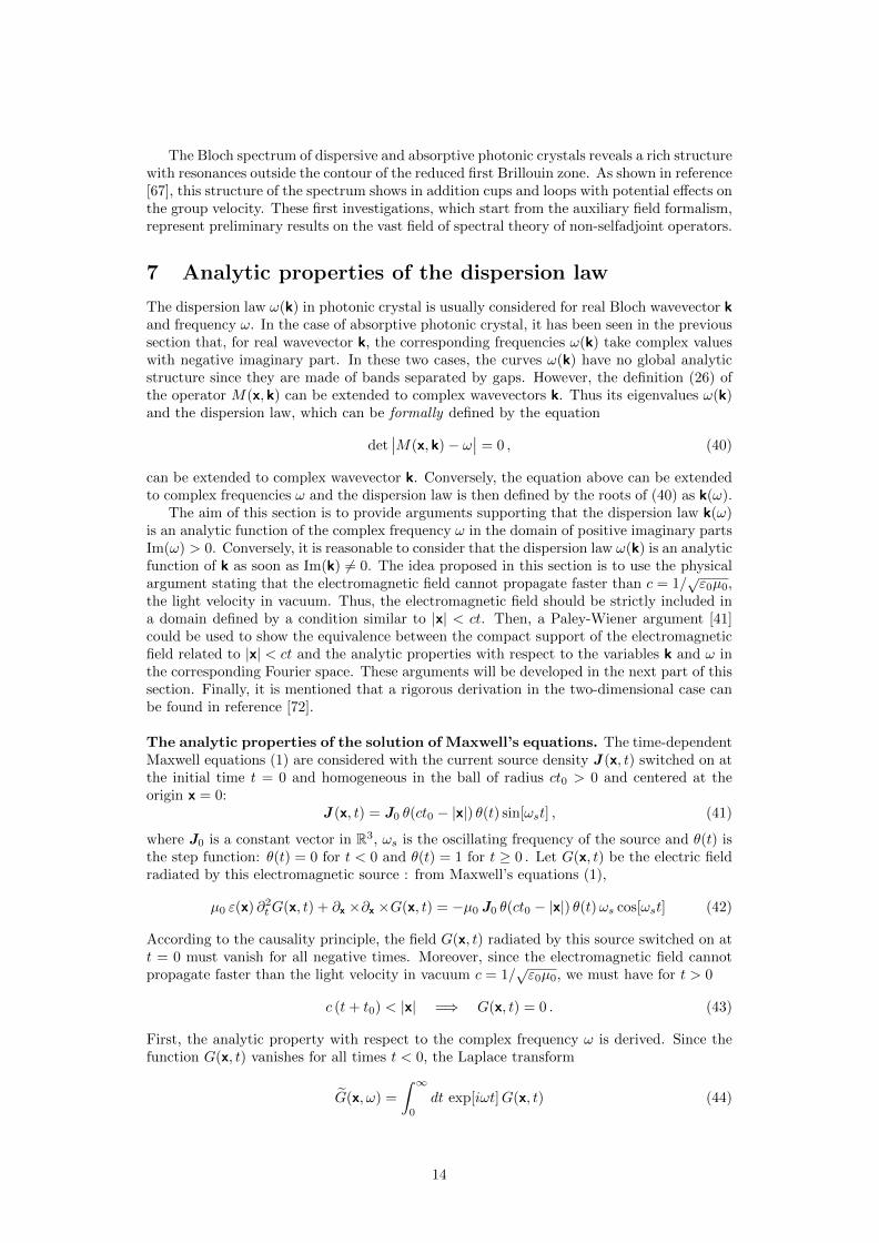
Figure 8 shows the first band (left panel) and the overlapping second and third bands(right panel). The first band is a skewed triangle which can be unambiguously related tothe reduced first Brillouin zone. Each edge of this triangle ΓXMΓ can be clearly identified:
12
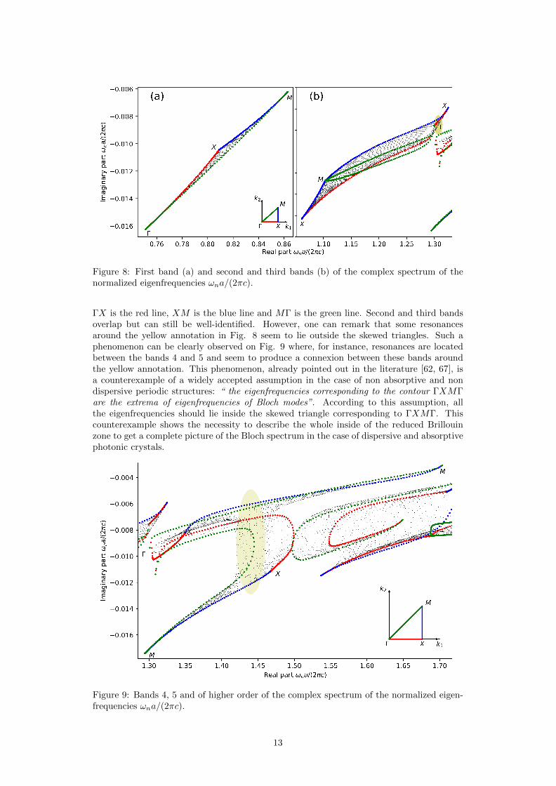
Figure 8: First band (a) and second and third bands (b) of the complex spectrum of thenormalized eigenfrequencies ωna/(2πc).
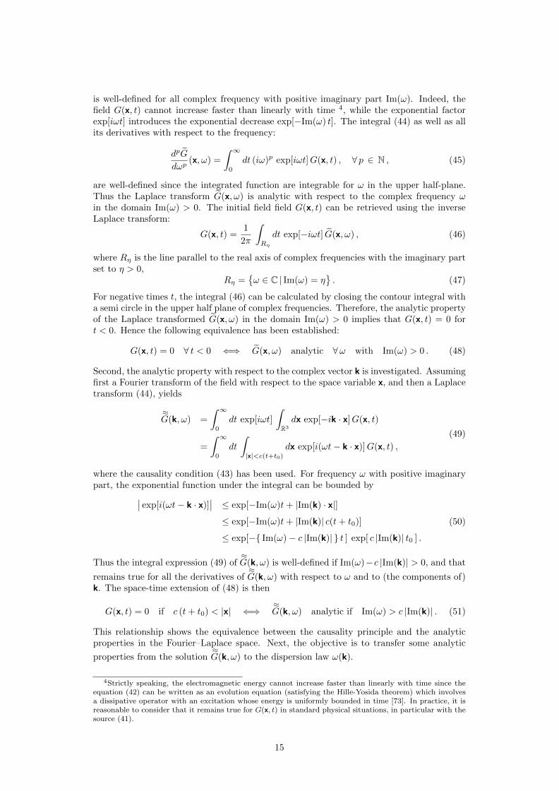
ΓX is the red line, XM is the blue line and MΓ is the green line. Second and third bandsoverlap but can still be well-identified. However, one can remark that some resonancesaround the yellow annotation in Fig. 8 seem to lie outside the skewed triangles. Such aphenomenon can be clearly observed on Fig. 9 where, for instance, resonances are locatedbetween the bands 4 and 5 and seem to produce a connexion between these bands aroundthe yellow annotation. This phenomenon, already pointed out in the literature [62, 67], isa counterexample of a widely accepted assumption in the case of non absorptive and nondispersive periodic structures: “ the eigenfrequencies corresponding to the contour ΓXMΓare the extrema of eigenfrequencies of Bloch modes”. According to this assumption, allthe eigenfrequencies should lie inside the skewed triangle corresponding to ΓXMΓ. Thiscounterexample shows the necessity to describe the whole inside of the reduced Brillouinzone to get a complete picture of the Bloch spectrum in the case of dispersive and absorptivephotonic crystals.
Figure 9: Bands 4, 5 and of higher order of the complex spectrum of the normalized eigen-frequencies ωna/(2πc).
13
The Bloch spectrum of dispersive and absorptive photonic crystals reveals a rich structurewith resonances outside the contour of the reduced first Brillouin zone. As shown in reference[67], this structure of the spectrum shows in addition cups and loops with potential effects onthe group velocity. These first investigations, which start from the auxiliary field formalism,represent preliminary results on the vast field of spectral theory of non-selfadjoint operators.
7 Analytic properties of the dispersion law
The dispersion law ω(k) in photonic crystal is usually considered for real Bloch wavevector kand frequency ω. In the case of absorptive photonic crystal, it has been seen in the previoussection that, for real wavevector k, the corresponding frequencies ω(k) take complex valueswith negative imaginary part. In these two cases, the curves ω(k) have no global analyticstructure since they are made of bands separated by gaps. However, the definition (26) ofthe operator M(x, k) can be extended to complex wavevectors k. Thus its eigenvalues ω(k)and the dispersion law, which can be formally defined by the equation
det∣∣M(x, k)− ω
∣∣ = 0 , (40)
can be extended to complex wavevector k. Conversely, the equation above can be extendedto complex frequencies ω and the dispersion law is then defined by the roots of (40) as k(ω).
The aim of this section is to provide arguments supporting that the dispersion law k(ω)is an analytic function of the complex frequency ω in the domain of positive imaginary partsIm(ω) > 0. Conversely, it is reasonable to consider that the dispersion law ω(k) is an analyticfunction of k as soon as Im(k) 6= 0. The idea proposed in this section is to use the physicalargument stating that the electromagnetic field cannot propagate faster than c = 1/
√ε0µ0,
the light velocity in vacuum. Thus, the electromagnetic field should be strictly included ina domain defined by a condition similar to |x| < ct. Then, a Paley-Wiener argument [41]could be used to show the equivalence between the compact support of the electromagneticfield related to |x| < ct and the analytic properties with respect to the variables k and ω inthe corresponding Fourier space. These arguments will be developed in the next part of thissection. Finally, it is mentioned that a rigorous derivation in the two-dimensional case canbe found in reference [72].
The analytic properties of the solution of Maxwell’s equations. The time-dependentMaxwell equations (1) are considered with the current source density J (x, t) switched on atthe initial time t = 0 and homogeneous in the ball of radius ct0 > 0 and centered at theorigin x = 0:
J (x, t) = J0 θ(ct0 − |x|) θ(t) sin[ωst] , (41)
where J0 is a constant vector in R3, ωs is the oscillating frequency of the source and θ(t) isthe step function: θ(t) = 0 for t < 0 and θ(t) = 1 for t ≥ 0 . Let G(x, t) be the electric fieldradiated by this electromagnetic source : from Maxwell’s equations (1),
µ0 ε(x) ∂2tG(x, t) + ∂x ×∂x ×G(x, t) = −µ0 J0 θ(ct0 − |x|) θ(t)ωs cos[ωst] (42)
According to the causality principle, the field G(x, t) radiated by this source switched on att = 0 must vanish for all negative times. Moreover, since the electromagnetic field cannotpropagate faster than the light velocity in vacuum c = 1/
√ε0µ0, we must have for t > 0
c (t+ t0) < |x| =⇒ G(x, t) = 0 . (43)
First, the analytic property with respect to the complex frequency ω is derived. Since thefunction G(x, t) vanishes for all times t < 0, the Laplace transform
G(x, ω) =
∫ ∞0
dt exp[iωt]G(x, t) (44)
14
is well-defined for all complex frequency with positive imaginary part Im(ω). Indeed, thefield G(x, t) cannot increase faster than linearly with time 4, while the exponential factorexp[iωt] introduces the exponential decrease exp[−Im(ω) t]. The integral (44) as well as allits derivatives with respect to the frequency:
dpG
dωp(x, ω) =
∫ ∞0
dt (iω)p exp[iωt]G(x, t) , ∀ p ∈ N , (45)
are well-defined since the integrated function are integrable for ω in the upper half-plane.Thus the Laplace transform G(x, ω) is analytic with respect to the complex frequency ωin the domain Im(ω) > 0. The initial field field G(x, t) can be retrieved using the inverseLaplace transform:
G(x, t) =1
2π
∫Rη
dt exp[−iωt] G(x, ω) , (46)
where Rη is the line parallel to the real axis of complex frequencies with the imaginary partset to η > 0,
Rη =ω ∈ C | Im(ω) = η
. (47)
For negative times t, the integral (46) can be calculated by closing the contour integral witha semi circle in the upper half plane of complex frequencies. Therefore, the analytic propertyof the Laplace transformed G(x, ω) in the domain Im(ω) > 0 implies that G(x, t) = 0 fort < 0. Hence the following equivalence has been established:
G(x, t) = 0 ∀ t < 0 ⇐⇒ G(x, ω) analytic ∀ω with Im(ω) > 0 . (48)
Second, the analytic property with respect to the complex vector k is investigated. Assumingfirst a Fourier transform of the field with respect to the space variable x, and then a Laplacetransform (44), yields
≈G(k, ω) =
∫ ∞0
dt exp[iωt]
∫R3
dx exp[−ik · x]G(x, t)
=
∫ ∞0
dt
∫|x|<c(t+t0)
dx exp[i(ωt− k · x)]G(x, t) ,
(49)
where the causality condition (43) has been used. For frequency ω with positive imaginarypart, the exponential function under the integral can be bounded by∣∣ exp[i(ωt− k · x)]
∣∣ ≤ exp[−Im(ω)t+ |Im(k) · x|]
≤ exp[−Im(ω)t+ |Im(k)| c(t+ t0)]
≤ exp[− Im(ω)− c |Im(k)| t ] exp[ c |Im(k)| t0 ] .
(50)
Thus the integral expression (49) of≈G(k, ω) is well-defined if Im(ω)−c |Im(k)| > 0, and that
remains true for all the derivatives of≈G(k, ω) with respect to ω and to (the components of)
k. The space-time extension of (48) is then
G(x, t) = 0 if c (t+ t0) < |x| ⇐⇒≈G(k, ω) analytic if Im(ω) > c |Im(k)| . (51)
This relationship shows the equivalence between the causality principle and the analyticproperties in the Fourier–Laplace space. Next, the objective is to transfer some analytic
properties from the solution≈G(k, ω) to the dispersion law ω(k).
4Strictly speaking, the electromagnetic energy cannot increase faster than linearly with time since theequation (42) can be written as an evolution equation (satisfying the Hille-Yosida theorem) which involvesa dissipative operator with an excitation whose energy is uniformly bounded in time [73]. In practice, it isreasonable to consider that it remains true for G(x, t) in standard physical situations, in particular with thesource (41).
15
The analytic properties of the dispersion law. The following section gives a reasoningthat enlightens the analytic properties of the dispersion law with respect to frequency inthe upper-half plane but it is not strictly speaking a rigorous mathematical proof. To ourknowledge, showing the analytic regularity of the dispersion law is still an open problemin mathematics for three-dimensional photonic crystals, but it has been established for thetwo-dimensional case in [72].
The solution G(x, t) of Maxwell’s equations can be retrieved from the inverse Fourier-Laplace transform applied to (49):
G(x, t) =1
(2π)4
∫Rη
dω
∫R3
dk exp[−iωt] exp[ik · x]≈G(k, ω) . (52)
Let k = |k| =√k · k be the modulus of k and ek = k/k the unit vector pointing in the direc-
tion of k. The integral over the wavevectors k is performed with respect to the wavenumberk and their directions ek on the unit sphere S:
G(x, t) =1
(2π)4
∫Rη
dω
∫S
dek
∫ ∞0
dk k2 exp[−iωt] exp[ik ek · x ]≈G(k, ω) . (53)
Let S+x be the hemisphere defined by
S+x =
ek ∈ S | ek · x > 0
. (54)
Then, the expression (53) can be written
G(x, t) =1
(2π)4
∫Rη
dω exp[−iωt]∫S+x
dek
∫Rdk k2 exp[ik ek · x ]
≈G(k, ω) . (55)
kekk4k3k2k1
xS+
x
k1
k2
Re(k)
Im(k)
k+1 k+
2 k+3 k+
4
k−1 k−
2 k−3 k−
4
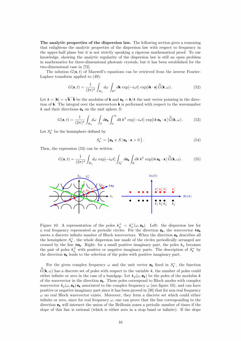
Figure 10: A representation of the poles k+p = k+
p (ω, ek). Left: the dispersion law fora real frequency represented as periodic circles. For the direction ek, the wavevector kekmeets a discrete infinite number of Bloch wavevectors. When the direction ek describes allthe hemisphere S+
x , the whole dispersion law made of the circles periodically arranged arecrossed by the line kek. Right: for a small positive imaginary part, the poles kp becomesthe pair of poles k±p with positive or negative imaginary parts. The description of S+
x bythe direction ek leads to the selection of the poles with positive imaginary part.
For the given complex frequency ω and the unit vector ek fixed in S+x , the function
≈G(k, ω) has a discrete set of poles with respect to the variable k, the number of poles couldeither infinite or zero in the case of a bandgap. Let kp(ω, ek) be the poles of the modulus kof the wavevector in the direction ek. These poles correspond to Bloch modes with complexwavevector kp(ω, ek) ek associated to the complex frequency ω (see figure 10), and can havepositive or negative imaginary part since it has been proved in [38] that for non real frequencyω no real Bloch wavevector exists. Moreover, they form a discrete set which could eitherinfinite or zero, since for real frequency ω, one can prove that the line corresponding to thedirection ek will intersect the union of the Brillouin zones a periodic number of times if theslope of this line is rational (which is either zero in a stop band or infinite). If the slope
16
is irrational these intersection points after K -translations to the first Brillouin zone formeda set that is dense in the first Brillouin zone, therefore the number of intersections in thatcase is again infinite or zero in a bandgap. This still holds by perturbation for frequency ωwith a small imaginary part. Since ek · x is positive, the integral over k can be calculatedby closing the line of real numbers by a semi-circle (with infinite radius) in the upper halfcomplex plane5. In that case, the set of Bloch wavevectors with positive imaginary partk+p (ω, ek) = k+
p (ω, ek) ek are picked up by closing the loop in the complex plane:
G(x, t) =2iπ
(2π)4
∫Rη
dω exp[−iωt]∫S+x
dek∑p
exp[ik+p (ω, ek) · x ] Res[k+p (ω, ek), ω] , (56)
where Res[k+p (ω, ek), ω] is the residue of k2 ≈G(kek, ω) at the pole k = k+p (ω). Then the
integral over all the directions ek in the hemisphere S+x is performed. As a result, all the
complex poles k+p (ω, ek), corresponding to the Bloch wavevectors k+p (ω, ek), are picked up
and the whole isofrequency dispersion law at the complex frequency ω is obtained: thisisofrequency dispersion law is periodic with respect to the wavevector k. Let k+0 (ω, ek) bethis isofrequency dispersion law restricted to the First Brillouin zone B (see figure 11). First,it is assumed that this isofrequency dispersion law is well-defined for for all direction ek, i.e.that the function k+0 (ω, ek) exists for all direction ek in the unit sphere S. This assumptionis correct for frequencies ω small enough at which, according to homogenization theory [74],the photonic crystal behaves like a homogeneous medium. Also, without loss of generality,no more than a single mode is assumed in each direction in the first Brillouin zone: inpractice, a finite sum over several modes in the first Brillouin could be considered.
Since the dispersion law k(ω) is L∗-periodic, the integral over S+x and the sum over p in
the expression (56) can be re-arranged as a periodic sum over the reciprocal lattice L∗ andthe unit sphere S:∫
S+x
dek∑p
exp[ik+p (ω) ek · x ] Res[k+
p (ω) ek, ω]
=∑
K∈L∗
∫S
dek exp[ik+0 (ω, ek) + K · x
]Res[k+0 (ω, ek) + K , ω
].
(57)
Let the function R#
[x, k+0 (ω, ek), ω
]be defined by
R#
[x, k+0 (ω, ek), ω
]=
i
(2π)3
∑K∈L∗
exp[ik+0 (ω, ek) + K · x
]Res[k+0 (ω, ek) + K , ω
]. (58)
This function has some properties of a Floquet-Bloch component: it is L∗-periodic withrespect to k+0 (ω, ek) and it satisfies the Bloch boundary conditions with respect to x. Withthis notation, the expression (56) of G(x, t) becomes
G(x, t) =
∫Rη
dω exp[−iωt]∫S
dekR#
[x, k+0 (ω, ek), ω
]. (59)
Now, from the analyticity property (48), the function R#
[x, k+0 (ω, ek), ω
]must be analytic
with respect to ω in the domain Im(ω) > 0 as soon as the expression above is valid. Thissuggests that the “dispersion law” k+0 (ω, ek) could be also analytic under the same conditionsif the function R#
[x, k+0 (ω, ek), ω
]could be “inverted”. In this aim, the Bloch boundary
condition is used: for a in the lattice L of the photonic crystal, the expression (58) implies
R#
[x + a, k+0 (ω, ek), ω
]= exp
[ik+0 (ω, ek) · a
]R#
[x, k+0 (ω, ek), ω
]. (60)
Hence the function exp[ik+0 (ω, ek) · a
]is analytic as soon as R#
[x, k+0 (ω, ek), ω
]does not
vanish. Now, for k+0 (ω, ek) in the first Brillouin zone, the function exp[ik+0 (ω, ek) ·a
]can be
5Notice that the Fourier transform of the source (41) is analytic of k, since the support of the source isincluded in the ball of radius ct0, and its exponential behavior is exp[±ikct0].
17
uniquely inverted and thus it is reasonable to consider that the “dispersion law” k+0 (ω, ek)is analytic with respect to ω. However, it is stressed that all these arguments are validunder the following conditions: the function k+0 (ω, ek) must exist for all direction ek in theunit sphere S and must remain in the First Brillouin zone B. These conditions are met forfrequencies ω small enough.
ω
k
k0(ω) k0(ω) + a1k0(ω) − a1
a1−a1
ω
k
ka(ω) ka(ω) + a1ka(ω) − a1
a1−a1
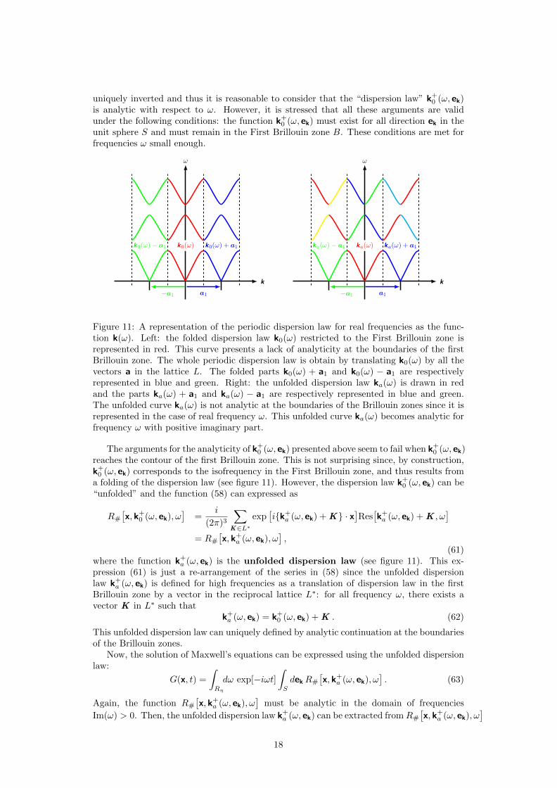
Figure 11: A representation of the periodic dispersion law for real frequencies as the func-tion k(ω). Left: the folded dispersion law k0(ω) restricted to the First Brillouin zone isrepresented in red. This curve presents a lack of analyticity at the boundaries of the firstBrillouin zone. The whole periodic dispersion law is obtain by translating k0(ω) by all thevectors a in the lattice L. The folded parts k0(ω) + a1 and k0(ω) − a1 are respectivelyrepresented in blue and green. Right: the unfolded dispersion law ka(ω) is drawn in redand the parts ka(ω) + a1 and ka(ω) − a1 are respectively represented in blue and green.The unfolded curve ka(ω) is not analytic at the boundaries of the Brillouin zones since it isrepresented in the case of real frequency ω. This unfolded curve ka(ω) becomes analytic forfrequency ω with positive imaginary part.
The arguments for the analyticity of k+0 (ω, ek) presented above seem to fail when k+0 (ω, ek)reaches the contour of the first Brillouin zone. This is not surprising since, by construction,k+0 (ω, ek) corresponds to the isofrequency in the First Brillouin zone, and thus results froma folding of the dispersion law (see figure 11). However, the dispersion law k+0 (ω, ek) can be“unfolded” and the function (58) can expressed as
R#
[x, k+0 (ω, ek), ω
]=
i
(2π)3
∑K∈L∗
exp[ik+a (ω, ek) + K · x
]Res[k+a (ω, ek) + K , ω
]= R#
[x, k+a (ω, ek), ω
],
(61)where the function k+a (ω, ek) is the unfolded dispersion law (see figure 11). This ex-pression (61) is just a re-arrangement of the series in (58) since the unfolded dispersionlaw k+a (ω, ek) is defined for high frequencies as a translation of dispersion law in the firstBrillouin zone by a vector in the reciprocal lattice L∗: for all frequency ω, there exists avector K in L∗ such that
k+a (ω, ek) = k+0 (ω, ek) + K . (62)
This unfolded dispersion law can uniquely defined by analytic continuation at the boundariesof the Brillouin zones.
Now, the solution of Maxwell’s equations can be expressed using the unfolded dispersionlaw:
G(x, t) =
∫Rη
dω exp[−iωt]∫S
dekR#
[x, k+a (ω, ek), ω
]. (63)
Again, the function R#
[x, k+a (ω, ek), ω
]must be analytic in the domain of frequencies
Im(ω) > 0. Then, the unfolded dispersion law k+a (ω, ek) can be extracted fromR#
[x, k+a (ω, ek), ω
]18
using the argument (60): hence it obtained that
exp[ik+a (ω, ek) + K · a
]= exp
[ik+0 (ω, ek) + K · a
], (64)
which is consistent with (62), but now the inversion of the exponential function must bedone in the way that preserves k+a (ω, ek) analytic when it spans the whole reciprocal space.Thus the unfolded dispersion law k+a (ω, ek) appears as the analytic continuation from thesmall frequencies ω of k+0 (ω, ek) in the first Brillouin zone.
Discussion. Arguments based on the causality principle have been proposed to supportthat the unfolded dispersion law k+(ω) ≡ k+a (ω, ek) is an analytic function of the frequencyin the domain of complex frequencies ω with positive imaginary part. This dispersion lawk+(ω) has been defined with a positive imaginary part. A similar dispersion law k−(ω) witha negative imaginary part could be defined using, instead of the hemisphere S+
x defined by(54), the hemisphere
S−x =ek ∈ S | ek · x < 0
. (65)
Indeed, in that case, the step from equation (55) to equation (56) is performed by closingthe real axis by a semi-circle in the lower half complex plane of number k, leading to pick upthe poles with negative imaginary parts. As a consequence, it is found that in the domainof frequencies ω with positive imaginary parts two distinct analytic dispersion laws k±(ω)exist, with k+(ω) = −k−(ω).
For small frequencies, the dispersion law k±(ω) is well-defined for all direction ek inthe unit sphere S. By analytic continuation, the dispersion law k±(ω) appears to be well-defined for all frequencies ω and for all directions ek, which could be considered as surprising.Indeed, for real frequencies and real wavevectors the periodicity of photonic crystal impliesthe presence of bandgaps and, more frequently, of stop bands (i.e. the absence of Blochmodes for certain directions ek). However, when considered in the complex plane, it appearsthat one can find a complex wavevector k for all frequency ω.
The present conclusions have been rigorously proved and numerically checked in the one-dimensional case in the reference [75]. In particular, it has been shown that the wavenumberk(ω) is an analytic function with respect to the frequency ω in the domain Im(ω) > 0 andthat its imaginary part cannot vanish (passivity requirement). Here, a similar result hasbeen found since the two analytic unfolded dispersion laws k±(ω) have keep the same sign fortheir imaginary part: hence the wavevectors k±(ω) cannot vanish. In the one-dimensionalcase [75], all these results have been confirmed numerically, for instance by checking thevalidity of the Kramers-Kronig relations.
It is stressed that the arguments presented in this section remain valid in the case ofdispersive and absorptive photonic crystals since it preserves the analytic nature with respectto the frequency.
Finally, the reciprocal dispersion law ω(k) has not been considered in this last section.Indeed, complex Bloch wavevector cannot be directly introduced with Fourier transformsince they imply exponential growing in the integrals. However, from the analytic properties
(51) of≈G(k, ω), it can be expected that a well-defined dispersion law ω(k) could have analytic
properties as soon as Im(k) 6= 0.
8 Conclusion
This chapter has been focused on fundamental definitions and properties of dispersion lawand group velocity in photonic crystals, including illustrations with numerical examples.This review has shown that numerous questions need to be investigated in the future. Thenumerical computation of the dispersion law becomes very challenging when the dispersionand absorption are introduced. The techniques based on the introduction of the auxiliaryfields [60, 38, 42] have been developed and numerically implemented [64, 67] and are now thebasic tool for the emerging topic of quasi-normal modes in photonics [65, 66]. It is stressedthat these numerical tools use only partial extension of Maxwell’s equations where the
19
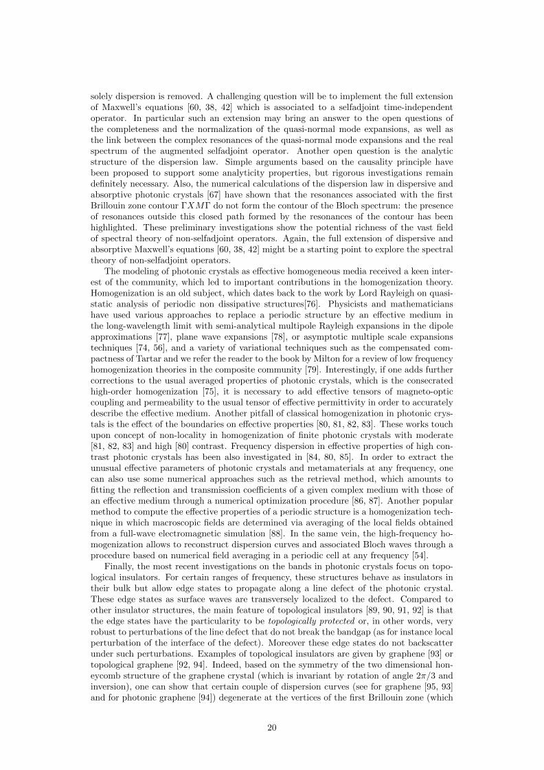
solely dispersion is removed. A challenging question will be to implement the full extensionof Maxwell’s equations [60, 38, 42] which is associated to a selfadjoint time-independentoperator. In particular such an extension may bring an answer to the open questions ofthe completeness and the normalization of the quasi-normal mode expansions, as well asthe link between the complex resonances of the quasi-normal mode expansions and the realspectrum of the augmented selfadjoint operator. Another open question is the analyticstructure of the dispersion law. Simple arguments based on the causality principle havebeen proposed to support some analyticity properties, but rigorous investigations remaindefinitely necessary. Also, the numerical calculations of the dispersion law in dispersive andabsorptive photonic crystals [67] have shown that the resonances associated with the firstBrillouin zone contour ΓXMΓ do not form the contour of the Bloch spectrum: the presenceof resonances outside this closed path formed by the resonances of the contour has beenhighlighted. These preliminary investigations show the potential richness of the vast fieldof spectral theory of non-selfadjoint operators. Again, the full extension of dispersive andabsorptive Maxwell’s equations [60, 38, 42] might be a starting point to explore the spectraltheory of non-selfadjoint operators.
The modeling of photonic crystals as effective homogeneous media received a keen inter-est of the community, which led to important contributions in the homogenization theory.Homogenization is an old subject, which dates back to the work by Lord Rayleigh on quasi-static analysis of periodic non dissipative structures[76]. Physicists and mathematicianshave used various approaches to replace a periodic structure by an effective medium inthe long-wavelength limit with semi-analytical multipole Rayleigh expansions in the dipoleapproximations [77], plane wave expansions [78], or asymptotic multiple scale expansionstechniques [74, 56], and a variety of variational techniques such as the compensated com-pactness of Tartar and we refer the reader to the book by Milton for a review of low frequencyhomogenization theories in the composite community [79]. Interestingly, if one adds furthercorrections to the usual averaged properties of photonic crystals, which is the consecratedhigh-order homogenization [75], it is necessary to add effective tensors of magneto-opticcoupling and permeability to the usual tensor of effective permittivity in order to accuratelydescribe the effective medium. Another pitfall of classical homogenization in photonic crys-tals is the effect of the boundaries on effective properties [80, 81, 82, 83]. These works touchupon concept of non-locality in homogenization of finite photonic crystals with moderate[81, 82, 83] and high [80] contrast. Frequency dispersion in effective properties of high con-trast photonic crystals has been also investigated in [84, 80, 85]. In order to extract theunusual effective parameters of photonic crystals and metamaterials at any frequency, onecan also use some numerical approaches such as the retrieval method, which amounts tofitting the reflection and transmission coefficients of a given complex medium with those ofan effective medium through a numerical optimization procedure [86, 87]. Another popularmethod to compute the effective properties of a periodic structure is a homogenization tech-nique in which macroscopic fields are determined via averaging of the local fields obtainedfrom a full-wave electromagnetic simulation [88]. In the same vein, the high-frequency ho-mogenization allows to reconstruct dispersion curves and associated Bloch waves through aprocedure based on numerical field averaging in a periodic cell at any frequency [54].
Finally, the most recent investigations on the bands in photonic crystals focus on topo-logical insulators. For certain ranges of frequency, these structures behave as insulators intheir bulk but allow edge states to propagate along a line defect of the photonic crystal.These edge states as surface waves are transversely localized to the defect. Compared toother insulator structures, the main feature of topological insulators [89, 90, 91, 92] is thatthe edge states have the particularity to be topologically protected or, in other words, veryrobust to perturbations of the line defect that do not break the bandgap (as for instance localperturbation of the interface of the defect). Moreover these edge states do not backscatterunder such perturbations. Examples of topological insulators are given by graphene [93] ortopological graphene [92, 94]. Indeed, based on the symmetry of the two dimensional hon-eycomb structure of the graphene crystal (which is invariant by rotation of angle 2π/3 andinversion), one can show that certain couple of dispersion curves (see for graphene [95, 93]and for photonic graphene [94]) degenerate at the vertices of the first Brillouin zone (which
20
is here hexagonal) where they cross conically on points referred in the literature as Diracpoints. Perturbing the dispersion curves at a Dirac point with a line defect that breaksthe PT symmetry (i.e. the composition of parity-inversion and time-reversal symmetries)of the crystal allows to open a gap (that could be only a local gap for the case of photonicgraphene see [94]). In addition, such a defect ensures the existence of topology protectededge states which are localized in this gap [94, 93].
References
[1] E. Yablonovitch, Inhibited spontaneous emission in solid-state physics and electronics,Phys. Rev. Lett. 58, 002059, (1987).
[2] J. Sajeev, Strong localization of photons in certain disordered dielectric superlattices,Phys. Rev. Lett. 58, 002486, (1987).
[3] V. P. Bykov, Spontaneous emission in a periodic structure, Soviet Journal of Experi-mental and Theoretical Physics. 35, 000269, (1972).
[4] C. Kittel, Introduction to Solid State Physics, 6th Edition. (John Wiley & Sons, 1986).
[5] E. Yablonovitch, T. J. Gmitter, and K. M. Leung, Photonic band structure: the face-centered-cubic case employing nonspherical atoms, Phys. Rev. Lett. 67, 002295, (1991).
[6] W. B. Russel, D. A. Saville, and W. R. Schowalter, Colloidal dispersions. (CambridgeUniversity Press, 1995).
[7] A. van Blaaderen, R. Ruel, and P. Wiltzius, Template-directed colloidal crystallization,Nature. 385, 000321, (1997).
[8] S. Y. Lin, J. G. Fleming, D. L. Hetherington, B. K. Smith, R. Biswas, K. M. Ho, M. M.Sigalas, W. Zubrzycki, S. R. Kurtz, and J. Bur, A three-dimensional photonic crystaloperating at infrared wavelengths, Nature. 394, 000351, (1998).
[9] J. G. Fleming and S.-Y. Lin, Three-dimensional photonic crystal with a stop band from1.35 to 1.95 µm, Opt. Lett. 64, 000049, (1999).
[10] S. Noda, K. Tomoda, N. Yamamoto, and A. Chutinan, Full three-dimensional photonicbandgap crystal at near-infrared wavelengths, Science. 289, 000604, (2000).
[11] S.-Y. Lin, J. G. Fleming, R. Lin, M. M. Sigalas, R. Biswas, and K. M. Ho, Completethree-dimensional photonic bandgap in a simple cubic structure, J. Opt. Soc. Am. B.18, 000032, (2001).
[12] A. Blanco, E. Chomski, S. Grabtchak, M. Ibisate, S. John, S. Leonard, C. Lopez,F. Meseguer, H. Miguez, J. P. Mondia, G. A. Ozin, O. Toader, and H. M. van Driel,Large-scale synthesis of a silicon photonic crystal with a complete three-dimensionalbandgap near 1.5 micrometres, Nature. 405, 000437, (2000).
[13] Y. A. Vlasov, X.-Z. Bo, J. C. Sturm, and D. J. Norris, On-chip natural assembly ofsilicon photonic bandgap crystals, Nature. 414, 000289, (2001).
[14] T. F. Krauss, R. M. De La Rue, and S. Brand, Two-dimensional photonic-bandgapstructures operating at near-infrared wavelengths, Nature. 383, 000699, (1996).
[15] J. Knight, T. Birks, P. Russell, and D. Atkin, All-silica single-mode optical fiber withphotonic crystal cladding, Opt. lett. 21, 001547, (1996).
[16] T. P. White, B. T. Kuhlmey, R. C. McPhedran, D. Maystre, G. Renversez, C. M.de Sterke, and L. Botten, Multipole method for microstructured optical fibers. i. for-mulation, J. Opt. Soc. Am. B. 19, 002322, (2002).
21
[17] B. T. Kuhlmey, T. P. White, G. Renversez, D. Maystre, L. C. Botten, C. M. de Sterke,and R. C. McPhedran, Multipole method for microstructured optical fibers. ii. imple-mentation and results, J. Opt. Soc. Am. B. 19, 002331, (2002).
[18] S. Guenneau, C. G. Poulton, and A. B. Movchan, Oblique propagation of elecromagneticand elastodynamic waves for an array of cylindrical fibres, Proc. R. Soc. A. 459, 002215,(2003).
[19] A. Nicolet, S. Guenneau, C. Geuzaine, and F. Zolla, Modeling of electromagnetic wavesin periodic media with finite elements, J. Comp. Appl. Math. 168, 000321, (2004).
[20] F. Zolla, G. Renversez, A. Nicolet, B. Kuhlmey, S. Guenneau, and D. Felbacq, Foun-dations of photonic crystal fibres. (Imperial College Press, London, 2005).
[21] C. Weisbuch, H. Benisty, S. Olivier, M. Rattier, C. J. M. Smith, and T. F. Krauss,Advances in photonic crystals, Physica Status Solidi. 221, 000093, (2000).
[22] C. R. B. Jamois, Wehrspohn, L. C. Andreani, C. Hermannd, O. Hess, and U. Gosele,Silicon-based two-dimensional photonic crystal waveguides, Nature. 383, 000699,(1996).
[23] S. Noda, A. Chutinan, and M. Imada, Trapping and emission of photons by a singledefect in a photonic bandgap structure, Nature. 407, 000608, (2000).
[24] Y. Akahane, T. Asano, B. S. Song, and S. Noda, High-q photonic nanocavity in atwo-dimensional photonic crystal, Nature. 425, 000944, (2003).
[25] S. Enoch, B. Gralak, and G. Tayeb, Enhanced emission with angular confinement fromphotonic crystals, Appl. Phys. Lett. 81, 001588, (2002).
[26] S. Enoch, G. Tayeb, P. Sabouroux, N. Guerin, and P. Vincent, A metamaterial fordirective emission, Phys. Rev. Lett. 89, 213902, (2002).
[27] P. Yeh, Electromagnetic propagation in birefringent layered media, J. Opt. Soc. Am.69, 000742, (1979).
[28] B. Gralak, S. Enoch, and G. Tayeb, Superprism effects and ebg antenna applications,Chapter 10 in Metamaterials: Physics and Engineering Explorations, Edited by N.Engheta and R. W. Ziolkowski, John Wiley and Sons. (2006).
[29] S. Enoch, B. Gralak, and G. Tayeb, The richness of the dispersion relation of elec-tromagnetic bandgap materials, IEEE transactions on antennas and propagation. 51,002659, (2003).
[30] B. Gralak, S. Enoch, and G. Tayeb, Anomalous refractive properties of photonic crys-tals, J. Opt. Soc. Am. A. 17, 001012, (2000).
[31] T. Decoopman, G. Tayeb, S. Enoch, D. Maystre, and B. Gralak, Photonic crystal lens:From negative refraction and negative index to negative permittivity and permeability,Phys. Rev. Lett. 97, 073905, (2006).
[32] W. Smigaj, B. Gralak, R. Pierre, and G. Tayeb, Antireflection gratings for a photonic-crystal flat lens, Opt. Lett. 341, 003532, (2009).
[33] G. Scherrer, M. Hofman, W. Smigaj, B. Gralak, X. Melique, D. Vanbesien, O. Lip-pens, C. Dumas, B. Cluzel, and F. de Fornel, Interface engineering for improved lighttransmittance through photonic crystal flat lenses, Appl. Phys. Lett. 97, 071119, (2010).
[34] J. B. Pendry, Negative refraction makes a perfect lens, Phys. Rev. Lett. 85, 003966,(2000).
22
[35] D. R. Smith, W. J. Padilla, D. C. Vier, S. C. Nemat-Nasser, and S. Schultz, Compositemedium with simultaneously negative permeability and permittivity, Phys. Rev. Lett.84, 004184, (2000).
[36] D. R. Smith, J. B. Pendry, and M. C. K. Wiltshire, Metamaterials and negative refrac-tive index, Science. 305, 000788, (2004).
[37] J. Joannopoulos, R. Meade, and J. Winn, Photonic crystals. (Princeton UniversityPress, 1995).
[38] A. Tip, A. Moroz, and J.-M. Combes, Band structure of absorptive photonic crystals,J. Phys. A: Mathematical and General. 33, 006223, (2000).
[39] A. Bensoussan, J.-L. Lions, and G. Papanicolaou, Asymptotic analysis for periodicstructures. (North-Holland, Amsterdam, 1978).
[40] P. Kuchment, Floquet Theory for Partial Differential Equations. (Birkhuser Verlag,1993).
[41] M. Reed and B. Simon, Methods of Modern Mathematical Physics. vol. II: FourierAnalysis, Self-Adjointness, (Academic Press, 1975).
[42] B. Gralak and A. Tip, Macroscopic Maxwells equations and negative index materials,J. Math. Phys. 51, 052902, (2010).
[43] B. Gralak, Analytic properties of the electromagnetic Greens function, J. Math. Phys.58, 071501, (2017).
[44] K. M. Leung and Y. F. Liu, Full vector wave calculation of photonic band structuresin face-centered-cubic dielectric media, Phys. Rev. Lett. 65, 002646, (1990).
[45] Z. Zhang and S. Satpathy, Electromagnetic wave propagation in periodic structures:Bloch wave solution of Maxwell’s equations, Phys. Rev. Lett. 65, 002650, (1990).
[46] K. Ho, C. Chan, and C. Soukoulis, Existence of photonic gap in periodic dielectricstructures, Phys. Rev. Lett. 65, 003152, (1990).
[47] K. M. Ho, C. T. Chan, C. M. Soukoulis, R. Biswas, and M. Sigalas, Photonic bandgaps in three dimensions: new layer-by-layer periodic structures, Solid State Commu-nications. 89, 000413, (1994).
[48] A. Chutinan and S. Noda, Effect of structural fluctuations on the photonic bandgapduring fabrication of a photonic crystal, J. Opt. Soc. Am. B. 16, 000240, (1999).
[49] V. Lousse, J.-P. Vigneron, X. Bouju, and J.-M. Vigoureux, Atomic radiation rates inphotonic crystals, Phys. Rev. B. 64, 201104(R), (2001).
[50] D. M. Whittaker, Inhibited emission in photonic woodpile lattices, Opt. Lett. 25,000779, (2000).
[51] S. G. Johnson and J. D. Joannopoulos, Block-iterative frequency-domain methods formaxwell’s equations in a planewave basis, Opt. Express. 8, 000173, (2001).
[52] comsol multiphysics, www.comsol.fr.
[53] G. Scherrer, M. Hofman, W. Smigaj, M. Kadic, T.-M. Chang, X. Melique, D. Lippens,O. Vanbesien, B. Cluzel, F. de Fornel, S. Guenneau, and B. Gralak, Photonic crystalcarpet: Manipulating wave fronts in the near field at 1.55µm, Phys. Rev. B. 88, 115110,(2013).
[54] R. Craster, J. Kaplunov, and A. Pichugin, High-frequency homogenization for periodicmedia, Proc. R. Soc. A. p. 20090612, (2010).
23
[55] T. Antonakakis, R. Craster, and S. Guenneau, High-frequency homogenization of zero-frequency stop band photonic and phononic crystals, New J. Phys. 15, 103014, (2013).
[56] S. Guenneau and F. Zolla, Homogenization of three-dimensional finite photonic crystals,Progress in Electromagnetics Research. 27, 000091, (2000).
[57] W. Smigaj and G. Gralak, Semianalytical design of antireflection gratings for photoniccrystals, Phys. Rev. B. 85, 035114, (2012).
[58] A. Moroz, Three-dimensional complete photonic-bandgap structures in the visible,Phys. Rev. Lett. 83, 005274, (1999).
[59] H. van der Lem and A. Moroz, Towards two-dimensional complete photonic band-gap structures below infrared wavelengths, J. Opt. A: Pure Applied Optics. 2, 000395,(2000).
[60] A. Tip, Linear absorptive dielectric, Phys. Rev. A. 57, 004818, (1998).
[61] A. Tip, Canonical formalism and quantization for a class of classical fields with appli-cation to radiative atomic decay in dielectric, Phys. Rev. A. 56, 005022, (1997).
[62] H. van der Lem, A. Tip, and A. Moroz, Band structure of absorptive two-dimensionalphotonic crystals, J. Opt. Soc. Am. B. 20, 001334, (2003).
[63] J.-M. Combes, B. Gralak, and A. Tip, Spectral properties of absorptive photonic crys-tals, Contemporary Mathematics Waves in Periodic and Random Media. 339, 1, (2003).
[64] A. Raman and S. Fan, Photonic band structure of dispersive metamaterials formulatedas a hermitian eigenvalue problem, Phys. Rev. Lett. 104, 087401, (2010).
[65] P. Lalanne, W. Yan, K. Vynck, C. Sauvan, and J.-P. Hugonin, Light interaction withphotonic and plasmonic resonances, Laser Photonics Rev. 2018, 1700113, (2018).
[66] W. Yan, R. Faggiani, and P. Lalanne, Rigorous modal analysis of plasmonic nanores-onators, Phys. Rev. B. 97, 205422, (2018).
[67] Y. Brule, B. Gralak, and G. Demesy, Calculation and analysis of the complex bandstructure of dispersive and dissipative two-dimensional photonic crystals, J. Opt. Soc.Am. B. 33, 000691, (2016).
[68] C. Geuzaine and J.-F. Remacle, Gmsh: a three-dimensional finite element mesh genera-tor with built-in pre- and post-processing facilities, International Journal for NumericalMethods in Engineering. 79, 001309, (2009).
[69] J. Webb and B. Forgahani, Hierarchal scalar and vector tetrahedra, IEEE Transactionson Magnetics. 29, 001495, (1993).
[70] P. Dular, C. Geuzaine, F. Henrotte, and W. Legros, A general environment for thetreatment of discrete problems and its application to the finite element method, IEEETransactions on Magnetics. 34, 003395, (1998).
[71] V. Hernandez, J. E. Roman, and V. Vidal, SLEPc: A scalable and flexible toolkit forthe solution of eigenvalue problems, ACM Transactions on Mathematical Software. 31,000351, (2005).
[72] H. Knorrer and E. Trubowitz, A directional compactification of the complex blochvariety, Commentarii Mathematici Helvetici. 65, 000114, (1990).
[73] R. Dautray and J.-L. Lions, Mathematical Analysis and Numerical Methods for Scienceand Technology. Volume 5 Evolution Problems I. (Springer, 2000).
[74] A. Bensoussan, J.-L. Lions, and G. Papanicolaou, Asymptotic analysis for periodicstructures. (North-Holland, 1978).
24
[75] Y. Liu, S. Guenneau, and B. Gralak, Artificial dispersion via high-order homogeniza-tion: magnetoelectric coupling and magnetism from dielectric layers, Proc. R. Soc. A.469, 20130240, (2013).
[76] L. Rayleigh, On the influence of obstacles arranged in rectangular order upon the prop-erties of a medium, Philosophical Magazine. 34, 481–502, (1892).
[77] R. C. McPhedran, C. Poulton, N. Nicorovici, and A. Movchan, Low frequency correc-tions to the static effective dielectric constant of a two-dimensional composite material,Proc. R. Soc. A. 452, 002231, (1996).
[78] P. Halevi, A. Krokhin, and J. Arriaga, Photonic crystal optics and homogenization of2d periodic composites, Phys. Rev. Lett. 82, 000719, (1999).
[79] G. Milton, The theory of composites. (Cambridge University Press, 2002).
[80] M. Silveirinha, Additional boundary condition for the wire medium, IEEE transactionson antennas and propagation. 54, 001766, (2006).
[81] R. Pierre and G. Gralak, Appropriate truncation for photonic crystals, J. Mod. Opt.55, 001759, (2008).
[82] W. Smigaj and B. Gralak, Validity of the effective-medium approximation of photoniccrystals, Phys. Rev. B. 77, 235445, (2008).
[83] V. A. Markel and I. Tsukerman, Current-driven homogenization and effective mediumparameters for finite samples, Phys. Rev. B. 88, 125131, (2013).
[84] D. Felbacq and G. Bouchitte, Homogenization of a set of parallel fibres, Waves inrandom media. 7, 000245, (1997).
[85] M. Silveirinha, Metamaterial homogenization approach with application to the charac-terization of microstructured composites with negative parameters, Phys. Rev. B. 75,115104, (2007).
[86] T. Koschny, P. Markos, D. R. Smith, and C. M. Soukoulis, Resonant and antiresonantfrequency dependence of the effective parameters of metamaterials., Phys. Rev. E. 68,065602(R), (2003).
[87] C. Menzel, C. Rockstuhl, T. Paul, F. Lederer, and T. Pertsch, Retrieving effectiveparameters for metamaterials at oblique incidence., Phys. Rev. B. 77, 195328, (2008).
[88] D. Smith and J. Pendry, Homogenization of metamaterials by field averaging, J. Opt.Soc. Am. B. 23, 000391, (2006).
[89] W. J. Chen, S. J. Jiang, X. D. Chen, B. Zhu, L. Zhou, Dong, J. W., and C. T. Chan,Experimental realization of photonic topological insulator in a uniaxial metacrystalwaveguide., Nat. Comm. 5, 005782, (2014).
[90] C. L. Kane and E. J. Mele, Z2 topological order and the quantum spin hall effect.,Phys. Rev. 14, 146802, (2005).
[91] S. Raghu and F. D. M. Haldane, Analogs of quantum-hall-effect edge states in photoniccrystals., Phys. Rev. A. 78, 033834, (2008).
[92] M. C. Rechtsman, J. M. Zeuner, Y. Plotnik, Y. Lumer, D. Podolsky, F. Dreisow, andA. Szameit, Photonic floquet topological insulators., Nature. 496, 000196, (2013).
[93] C. L. Fefferman, J. P. Lee-Thorp, and M. I. Weinstein, Honeycomb schrodinger opera-tors in the strong binding regime, Communications on Pure and Applied Mathematics.71, 001178, (2018).
25
[94] J. P. Lee-Thorp, M. I. Weinstein, and Y. Zhu, Elliptic operators with honeycomb sym-metry: Dirac points, edge states and applications to photonic graphene, available onarxiv at https: // arxiv. org/ abs/ 1710. 03389 . (2017).
[95] P. R. Wallace, The band theory of graphite, Phys. Rev. 71, 000622, (1947).
26


