arX

iv:c

ond-

mat

/980

5108

v1 [

cond

-mat

.sup

r-co

n] 1

1 M

ay 1

998

Electron–phonon interaction and optical spectra of metals

H. J. Kaufmann∗

Interdisciplinary Research Centre in Superconductivity, University of Cambridge, Madingley

Road, Cambridge CB3 0HE, UK and Department of Earth Sciences, University of Cambridge,

Downing Street, Cambridge CB2 3EQ, UK.

E. G. MaksimovP. N. Lebedev Physical Institute, 117924 Moscow, Russia.

E. K. H. SaljeInterdisciplinary Research Centre in Superconductivity, University of Cambridge, Madingley

Road, Cambridge CB3 0HE, UK and Department of Earth Sciences, University of Cambridge,

Downing Street, Cambridge CB2 3EQ, UK.

Abstract

Observed optical reflectivity in the infrared spectral region is compared with

theoretical predictions in a strongly coupled electron–phonon system. Start-

ing from a Frohlich Hamiltonian, the spectral functions and their temperature

dependence are derived. A full analysis including vertex corrections leads to

an expression for the optical conductivity σ(ω) which can be formulated in

terms of the well known optical conductivity for a quasi–isotropic system with-

out vertex corrections. A numerical comparison between the full result and

the so–called “extended” Drude formula, its weak coupling expansion, show

little difference over a wide range of coupling constants. Normal state optical

spectra for the high-Tc superconductors YBa2Cu3O7 and La2−xSrxCuO4 at

optimal doping are compared with the results of model calculations. Taking

the plasma frequency and ǫ∞ from band structure calculations, the model has

only one free parameter, the electron–phonon coupling constant λ. In both

materials the overall behaviour of the reflectivity can be well accounted for

over a wide frequency range. Systematic differences exist only in the mid–

infrared region. They become more pronounced with increasing frequency,

which indicates that a detailed model for the optical response should include

temperature dependent mid–infrared bands.

Keywords: optical properties, electron–phonon interaction, high–Tc super-

conductorsTypeset using REVTEX

∗corresponding author; Tel. +44-1223-333409, Fax +44-1223-333450, e-mail hjk22@cus.cam.ac.uk

1

I. INTRODUCTION

The optical spectra of metals in the infrared (IR) spectral region depend sensitively onthe interaction between electrons and phonons. Deviations from the theoretical spectrumwithout any phonon contribution stem from the so–called Holstein mechanism [1] in whichthe incident photon is absorbed in a second–order process involving creation of both a phononand an electron–hole pair. The detailed description of this mechanism was given by Allen[2]. Despite the fact that the physical mechanism of electron–phonon coupling is rather wellunderstood for almost three decades, little process was made in the systematic experimentalstudy of coupling effects in optical (IR) spectra [3], nor has the phenomenology been exploredbeyond the lowest order effects. The lack of systematic experimental investigations appearsto be related to the following two reasons:

Firstly, historically measurements of optical spectra of metals where limited to photonenergies ω >

∼ 0.05 eV [3]. We shall argue in this paper that the effects of the electron–phononinteraction on the optical spectra of ordinary metals are rather weak at these energies. Theoptical conductivity in this spectral range can usually be described in the framework of theDrude formula

σ(ω) =ω2

pl

4π

1

−iω + 1/τ(1)

where 1/τ is the relaxation rate of electrons due to their interaction with impurities andphonons. It can be calculated using the commonly adapted Bloch–Gruneisen–type formula.

Secondly, the measurements of the optical conductivity are complicated in ordinary met-als by the anomalous skin effect which is mostly present at low temperatures and in thefar–infrared (FIR) spectral region. It leads to serious difficulties in the interpretation ofreflectivity and absorbtivity measurements. Only a few observations [4,5] are known to uswhere Holstein processes where identified in the normal state of ordinary metals.

The discovery of the high-Tc superconductors (HTSC) has dramatically changed theexperimental situation. First of all, the experimental methods were improved radically byextending the accessible energy range down to ≈ 10 cm−1 and by increasing the accuracyof the measurements. Secondly, it appears that HTSC systems allow the observation of theelectron–phonon interaction in the optical spectra more easily and more clearly than it waspossible in the ordinary metals. Thirdly, there is no anomalous skin effect in these systemsfor light with electric field parallel to the Cu–O planes.

It is the purpose of this paper to review the theoretical situation. We then extend thetreatment of the Frohlich Hamiltonian to include vortex corrections. Theoretical predictionsare then compared with experimental observations following earlier attempts to connectthe IR reflectivity and absorption spectra of HTSCs with features of strongly interactingelectron–phonon systems [6–8].

We shall show that most but not all observations can be described rather well withinsuch a scheme and identify some pertinent open questions.

2

II. DERIVATION OF THE OPTICAL CONDUCTIVITY IN THE FRAMEWORK

OF THE FROHLICH HAMILTONIAN

We start from the description of metals with electron–phonon interaction by the standardFrohlich Hamiltonian

H =∑

k,i

ǫk,i c†k,i ck,i +

∑

k,q,i,i′,λ

gk(q, i, i′, λ) c†k,i ck+q,i′ × (2)

×(

b†qλ + b−qλ

)

+∑

q,λ

ωqλb†qλ bqλ .

Here the first term is the kinetic energy of an electron with given momentum k and bandindex i, the last term is the energy of the phonon with momentum q and mode λ. Thesecond term represents the electron–phonon interaction, where gk(q, i, i′, λ) is the matrixelement of this interaction. The use of this Hamiltonian for the self–consistent calculationof the electron and phonon Green’s functions cannot be rigourously justified in the generalcase. It was shown [9–11] that this Hamiltonian can be used for the calculation of theinfluence of the electron–phonon interaction on the electronic properties for systems whereno low–energy collective excitations of electrons are present. First–principle calculations[10] of the physical properties of a number of ordinary metals have shown that the FrohlichHamiltonian is a very good starting point for the analysis of all features related to electron–phonon interactions. In HTSC materials we can not expect this Hamiltonian to describethe optical response completely because additional low energy excitations (e. g. spin and/orcharge excitations) occur. However, these excitations contribute little to the general trendof the “anomalous” optical properties of HTSC systems at high energies and are simplyignored in this study. The question we wish to answer here is the following: to what extendcan observed optical spectra in the normal state be understood in terms of the most simplemodel of electron–phonon interaction as represented by equation (2).

The many–body electron–phonon interaction are usually calculated by Green’s functionmethod [12]. Let us introduce the electron and phonon one–particle thermodynamic Green’sfunctions

Gi(k, τ) = −〈Tτ c†k,i(τ) ck,i(0)〉 (3)

and

Dλ(q, τ) = −〈Tτ b†qλ(τ) bqλ(0)〉 . (4)

The Wick operator Tτ reorders the operators following it in such a way that τ increases fromright to left. For non–interacting particles the Fourier components of the Green’s functions,Gi(k, iωn) and Dλ(q, iων), have the very simple form

G0i (k, iωn) =

1

iωn − ǫk,i(5)

and

D0λ(q, iων) =

(

1

iων − ωqλ−

1

iων + ωqλ

)

. (6)

3

Here iωn = (2n + 1)πT and iων = 2νπT are the Matsubara frequencies for fermions andbosons, respectively, and T is the temperature. The value ǫk,i is the electron band energyand, correspondingly, ωqλ is the phonon energy for the λth mode. In the following we donot consider the renormalisation of the phonon Green’s function due to the electron–phononinteraction. For convenience we present the phonon function Dλ(q, iων) in the spectral form

Dλ(q, iων) =1

π

∞∫

0

dΩ Im Dλ(q, Ω)(

1

iων − Ω−

1

iω + Ω

)

. (7)

For the non–interacting case the spectral density ImDλ(q, Ω) has the form

Im D0λ(q, Ω) = π δ(Ω− ωqλ) . (8)

In the following we tread the spectral function Im Dλ(q, Ω) as an experimental quantityand calculate the influence of the electron–phonon interaction on the electronic properties.These properties are reflected in the one–particle electron Green’s function and the opticalconductivity σαβ(ω). The one–particle Green’s function for electrons in the presence of theelectron–phonon interaction [13] can be written as

G−1(k, iωn) = G−10 (k, iωn)− Σ(k, iωn) (9)

where Σ(k, iωn) is the electron self–energy part. One of the main results of Migdal [13] isthat the electron self–energy can be calculated using the simplest first–order approximationin the electron–phonon interaction, neglecting all vertex corrections as being small of theorder of ωD/ǫF. Here ωD is a characteristic phonon energy and ǫF is the Fermi energy of theelectrons. An analytical expression of Σ(k, iωn) is

Σi(k, iωn) = −T∑

ων

∑

k′,i′,λ

|gk(k− k′, i, i′, λ)|2Dλ(k− k′, iων) × (10)

×G(k′, iωn − iων) .

The summation over the momentum k′ is represented in integral form

∑

k,i

=∑

i

∞∫

−∞

dǫ∑

k

δ(ǫ− ǫk,i) (11)

so that Σi(k, iωn) becomes

Σi(k, iωn) = −T∑

ων

∞∫

−∞

dǫ∑

k′,i′,λ

|gk(k− k′, i, i′, λ)|2δ(ǫ− ǫk′,i′)× (12)

×

∞∫

0

dΩ Im Dλ(k− k′, Ω) G(k′, iωn − iων)×

×(

1

iων − Ω−

1

iων + Ω

)

.

The analysis of (12), as performed by Migdal, shows that the essential values of iωn and iων

are of order ωD. This means that small frequencies of order ωD are also significant for ǫ. In

4

this case ǫ can be neglected in δ(ǫ− ǫk,i). The electron Green’s function is used in the formgiven by Eq. (5) leading to

Σi(k, iωn) = −T∑

ων

∑

k′

δ(ǫk′)

∞∫

0

dΩ α2i (k,k′, Ω)F (Ω)

(

1

iων − Ω−

1

iων + Ω

)

× (13)

×

∞∫

−∞

dǫ1

iωn − iων − ǫ,

where the spectral function of the electron–phonon interaction

α2i (k,k′, Ω)F (Ω) =

∑

i′,λ

|gk(k− k′, i, i′, λ)|2Im Dλ(k− k′, Ω) (14)

was introduced. The sum over the ων = 2πνT can be easily performed with the result

− T∑

ων

(

1

iων − Ω−

1

iων + Ω

)

1

iωn − iων − ǫ= (15)

=N(Ω) + 1− f(ǫ)

iωn − Ω− ǫ+

N(Ω) + f(ǫ)

iωn + Ω− ǫ,

where N(Ω) and f(ǫ) are the Bose and Fermi function, respectively. To obtain the one–particle Green’s function describing the electron excitation spectrum we use the analyticcontinuation of the self–energy on the imaginary axis ω. This can easily be done by changingiωn in Eq. (15) to ω. Consequently, the final expression for the self–energy reads

ΣR,Ai (k, ω) =

∞∫

0

dΩ∑

k′

δ(ǫk′) α2i (k,k′, Ω)F (Ω)L(ω ± iδ, Ω) , (16)

where

L(ω ± iδ, Ω) =

∞∫

−∞

dǫ

[

N(Ω) + 1− f(ǫ)

ω − Ω− ǫ± iδ+

N(Ω) + f(ǫ)

ω + Ω− ǫ± iδ

]

. (17)

The function ΣR (A)(k, ω) denotes the retarded (advanced) self–energy which is an analyticalfunction of the variable ω in the upper (lower) half of the complex plane. The integral in(17) can be evaluated analytically, yielding

L(ω, Ω) = −2πi[

N(Ω) +1

2

]

+ Ψ(

1

2+ i

Ω− ω

2πT

)

−Ψ(

1

2− i

Ω + ω

2πT

)

, (18)

where Ψ(z) is the digamma function. The self–energy ΣR,Ai (k, ω) expressed by Eq. (16)

depends only on the direction of the momentum k on the Fermi surface. It is convenientto present this dependence by expanding all functions involved in this expression over thecomplete and orthonormal set of functions introduced by Allen [14]. These so–called “Fermisurface harmonics”, Ψj(k), satisfy the condition

5

∑

k

Ψj(k)Ψj′(k) δ(ǫk − ǫ) = δjj′N(ǫ) , (19)

where

N(ǫ) =∑

k

δ(ǫk − ǫ) . (20)

In terms of this set we write

ΣR,Ai (k, ω) =

∑

j

ΣR,Ai,j (ω)Ψj(k) (21)

GR,Ai (k, ω) =

∑

j

GR,Ai,j (ǫk, ω)Ψj(k) (22)

α2j,j′(k, Ω)F (Ω) =

∑

j,j′

∑

k′,λ

δ(ǫk′)

|gk′(k− k′, i, i′, λ)|2Im Dλ(k− k′, ω)

jj′× (23)

×Ψj(k)Ψj′(k′) .

It follows from Eqs. (21-23) that the self–energy coefficients ΣR,Ai,j (ω) are given by

ΣR,Ai,j (ω) =

∑

j′

∞∫

0

dΩ α2j,j′(Ω)F (Ω)L(ω ± iδ, Ω) , (24)

where

α2j,j′(Ω)F (Ω) =

1

N(0)

∑

k

∑

k′

δ(ǫk)δ(ǫk′)α2(k,k′, Ω)F (Ω)Ψj(k)Ψj′(k′) . (25)

Here N(0) denotes the density of electron states on the Fermi surface. The first Fermiharmonic is Ψ0(k) = 1 and the function

α20,0(Ω)F (Ω) =

1

N(0)

∑

k

∑

k′

δ(ǫk)δ(ǫk′)α2(k,k′, Ω)F (Ω) (26)

is obviously the well known Eliashberg spectral function which determines the superconduc-tivity of metals in the simple s–pairing case. Introducing the real and imaginary parts ofthe self–energy, Σ1(k, ω) and Σ2(k, ω), respectively, the Green’s function becomes

G−1(k, ω + iδ) = ω − ǫk − Σ1(k, ω + iδ)− iΣ2(k, ω + iδ) . (27)

The pole of the Green’s function determines the spectrum of one–particle excitations. Atsmall energies Eq. (27) can be rewritten as

G−1(k, ω + iδ) = ω

(

1−∂Σ1(k, ω)

∂ω

∣

∣

∣

∣

∣

ω=0

)

− iΣ2(k, ω + iδ) . (28)

Then the pole of G occurs at ω0, which is given by

6

ω0 = Ek −i

2τk, (29)

Ek =

(

1−∂Σ1(k, ω)

∂ω

)−1

ǫk , (30)

1

2τk= −

(

1−∂Σ1(k, ω)

∂ω

)−1

Σ2(k, Ek) . (31)

Here

λk = −∂Σ1(k, ω)

∂ω

∣

∣

∣

∣

∣

ω=0

(32)

describes the change of the effective mass of the electron, while 12τk

describes their relaxationrate. All functions can be rewritten in terms of Fermi harmonics and the spectral functionα2

j,j′(Ω)F (Ω). We shall turn to this problem later when we discuss the conductivity of metalsin the presence of electron–phonon interaction.

As usual we write the conductivity of a metal in the presence of electron–phonon inter-action in terms of the analytically continued electromagnetic kernel Kαβ(ω),

σαβ(ω) =e2Kαβ(ω)

4πiω, (33)

which, in turn, is expressed through the one–particle Green’s function Gi(k, ω) and cor-responding vertex function Γβ . In the framework of the thermodynamical theory of theperturbations the expression for Kαβ(ω) is

Kαβ(iωn) = T∑

ωn′

∑

k′

υαk′ G(k′, iωn′)G(k′, iωn′ + iω)× (34)

×Γβ(k′, iωn′, iωn′ + iω) ,

where υαk′ is the α–component of the electron velocity. Using the ladder diagram approxi-

mation the equation for the vertex function is written as [1]

Γβ(k′, iωn′, iωn′ + iωn) = υβk′ + T

∑

k′′,n′′

|〈gk′′(k′ − k′′, i, i′, λ)〉|2× (35)

×Dλ(k′ − k′′, iωn′ − iωn′′)G(k′′, iωn′′)G(k′′, iωn′′ + iωn)×

×Γβ(k′′, iωn′′, iωn′′ + iωn) .

Before we solve Eqs. (34) and (35) we simplify them somewhat. Firstly, as the conductivityof any metal in the absence of a magnetic field can be diagonalised in the appropriaterepresentation we omit in the following the indices α and β considering the conductivity as ascalar. This is done bearing in mind that the absolute value of the conductivity in non–cubiccrystals is anisotropic and that the corresponding functions determining the temperatureand frequency dependence of σ(ω, T) reflect this anisotropy. Secondly, we omit the electronband indexes taking into account that interband transitions can be calculated separately ifneeded. We also omit the electron spin index multiplying by two the sum over the electronmomentum k. After that Eq. (35) is rewritten in a simplified form

7

Γx(k′, iωn′, iωn′ + iωn) = υx

k′ + 2T∑

k′′

∑

n′′

υxk′′

∞∫

−∞

dǫ δ(ǫ− ǫk′′)× (36)

×1

π

∞∫

0

dΩ α2(k′,k′′)F (Ω)×

×(

1

iωn′ − iωn′′ − Ω−

1

iωn′ − iωn′′ + Ω

)

×

×G(k′′, iωn′′)G(k′′, iωn′′ + iωn)×

×Γx(k′′, iωn′′, iωn′′ + iωn) .

To establish some important steps in the derivation of the general formula for σ(ω) weconsider, as a first step, the case where the vertex correction to the bare vertex Γx

k can beneglected. Then the expression for the electromagnetic response kernel K(iωn) becomes

Kxx(iωn) = 2T∑

k′

∑

ωn′

∞∫

−∞

dǫ δ(ǫ− ǫk′′)(υxk′)2 × (37)

×G(k′, iωn′)G(k′, iωn′ + iωn) .

We can now use the Poisson summation formula

∞∑

n=−∞

F (iωn) = −1

2πiT

∫

C

dωF (ω)

eω

T + 1′ (38)

where the contour C encircles the imaginary ω–axis. After that we expand the ω–contourto infinity, picking up contributions from the singularities of our integrand at iωn = ǫk′

and iωn = ǫk′ − iωn. As a result we find after rather lengthy but simple calculation theanalytically continued electromagnetic kernel as

K(ω) = 2∑

k′

(υxk′)2

∞∫

−∞

dǫ δ(ǫ− ǫk′′)

∞∫

−∞

dω′ × (39)

×

(

tanh

(

ω′

2T

)

− tanh

(

ω′ + ω

2T

))

×

×ΠRA0 (k′, ω′, ω) .

Here ΠRA0 (k′, ω′, ω) has the form

ΠRA0 (k′, ω′, ω) = GR(k′, ω′ + ω)GA(k′, ω′) , (40)

where GR(k′, ω′ + ω) and GA(k′, ω′) are the retarded and advanced Green’s function, re-spectively. Their self–energy parts are given by Eqs. (16 - 18). Just as in the case of theone–particle Green’s function the relevant values of ω are small in comparison to the Fermienergy, the value of ǫ in δ(ǫ− ǫk) can be neglected, and the integration over ǫ can be carriedout. As result we find for the conductivity

8

σ(ω) =e2

4πiω

∑

k

(υxk)

2δ(ǫk)

∞∫

−∞

dω′

(

tanh

(

ω′ + ω

2T

)

− tanh

(

ω′

2T

))

× (41)

×Π0(kF, ω′, ω) ,

where the function Π0(kF, ω′, ω) depends on the position of the momentum kF on the Fermisurface and is given by

Π0(kF, ω′, ω) =1

ω + ΣR(kF, ω + ω′)− ΣA(kF, ω′). (42)

For the quasi–isotropic case we get, of course, the well known result for the opticalconductivity [14,15]

σ(ω) =ω2

pl

4πiω

∞∫

−∞

dω′

(

tanh

(

ω′ + ω

2T

)

− tanh

(

ω′

2T

))

Π0(ω, ω′) , (43)

where the plasma frequency of electrons ωpl is

ω2pl = 2e2

∑

k

(υxk)

2δ(ǫk) (44)

and the function Π0(ω, ω′) is

Π0(ω, ω′) =1

ω + ΣR(ω + ω′)− ΣA(ω′) + iτimp

. (45)

Here we introduced the relaxation rate from impurity scattering 1τimp

.

For the anisotropic case we should expand all functions under the integral in Eq. (41)over the Fermi harmonics. The value (υx

k)2 is just the square of the Fermi harmonic of the

order N = 1 (for details see Ref. [14]). The expansion of the function Π0(kF, ω′, ω) can bewritten as

Π0(kF, ω′, ω) =∑

j

Πj(ω′, ω)Fj(kF) . (46)

The non–zero result for the conductivity will arise from the first harmonic, Fj(kF) = 1, andfrom the harmonics with even order N ≥ 2. The first harmonic gives the same result asfound for the isotropic case. An example of a higher harmonic is the one which transformsas the representation Γ12 of the crystal symmetry. It has the form

ΨΓ12

j =v2

yx − v2xy

⟨

(v2x − v2

y)2⟩1/2

. (47)

At this point we are not certain to which extent the higher harmonics are relevant in HTSCsystems but it is known that their influence is small in normal metals. This question shouldbe considered in more detail but is beyond the scope of this paper.

9

While the analytic continuation of Eqs. (33), (34) in the zero–order approximation andabsence of the vertex function Γ(k, iωn, iωm) is straightforward, it becomes a non–trivialtask in the presence of Γ(k, iωn, iωm). The difficulty arises from the existence of a manifoldof functions which can be obtained as a result of analytical continuation for one variablewhile another is fixed. However, this difficulty can be avoided by changing, as above, thesum over the Matsubara frequencies to a contour integral. The contour consists of (three)circuits around the imaginary axis of the variable ω′, avoiding all poles and branch cuts ofthe integrand. Using the methods developed in Refs. [1,16] we obtain

σ(ω) =2

4πiω

∑

k

∞∫

−∞

dǫ δ(ǫ− ǫk)υxk

∞∫

−∞

dω′

2πi

(

tanh

(

ω′ + ω

2T

)

− tanh

(

ω′

2T

))

× (48)

×ΠRA0 (k, ω′, ω)Γx(k, ω′, ω)

and

Γx(k, ω′, ω) = υxk + 2

∑

k′

∞∫

−∞

dǫ δ(ǫ− ǫk′)

∞∫

−∞

dω′′

2πi× (49)

×

[

tanh

(

ω′′ + ω

2T

)

λkk′(ω′ − ω′′ + iδ)− tanh

(

ω′′

2T

)

λkk′(ω′′ − ω′ − iδ)+

+coth

(

ω′ − ω′′

2T

)

(λkk′(ω′′ − ω′ + iδ)− λkk′(ω′ − ω′′ − iδ))

]

×

×ΠRA0 (k′, ω′′, ω)Γx(k

′, ω′′, ω) ,

where the function

λkk′(ω) =

∞∫

0

dΩ α2(k,k′, Ω)F (Ω)[

1

ω − Ω−

1

ω + Ω

]

(50)

was introduced. Taking into account that apart from Π0(k′, ω′′, ω) all functions under the

integral on the right–hand side of Eq. (49) depend only weakly on the variable ǫk′ we canintegrate over this variable and find

Γx(kF, ω′, ω) = υxk +

∑

k′

δ(ǫk′)

∞∫

−∞

dω′′ Π0(k′F, ω′′, ω)× (51)

× [I(ω′ − iδ, Ω, ω′′)− I(ω′ + ω + iδ, Ω, ω′′)] Γx(k′F, ω′′, ω) .

Here Π0(k′F, ω′′, ω) is defined by Eq. (42) and I(ω, Ω, ω′) is

I(ω, Ω, ω′) =1− f(ω′) + N(Ω)

ω − Ω− ω′+

f(ω′) + N(Ω)

ω + Ω− ω′. (52)

At this stage it is useful to introduce a new function γx(kF, ω′, ω),

γx(kF, ω′, ω) = Π0(kF, ω′, ω)Γx(kF, ω′, ω) . (53)

10

In terms of this function the conductivity can be expressed as

σ(ω) =2

4πiω

∑

k

δ(ǫk)υxk

∞∫

−∞

dω′

(

tanh

(

ω′ + ω

2T

)

− tanh

(

ω′

2T

))

× (54)

×γx(kF, ω′, ω) .

For γx(kF, ω′, ω) one can write the equation

ωγx(kF, ω′, ω) = υxk +

∑

k′

δ(ǫk′)

∞∫

0

dΩ α2(k,k′, Ω)F (Ω)× (55)

×

∞∫

−∞

dω′′ [I(ω′ − iδ, Ω, ω′′)− I(ω′ + ω + iδ, Ω, ω′′)]×

×(

γx(k′F, ω′′, ω)− γx(kF, ω′, ω)

)

.

Now we use the expansion of the functions in Eq. (55) in Fermi harmonics. This yields

ωγj(ω′, ω) =

⟨

υ2x

⟩1/2δjx +

∑

j′

∞∫

0

dΩ × (56)

×

∞∫

−∞

dω′′ [I(ω′ − iδ, Ω, ω′′)− I(ω′ + ω + iδ, Ω, ω′′)]×

×

α2jj′(Ω)F (Ω)γj′(ω

′′, ω)−∑

j′′Cjj′j′′α

2j′′0(Ω)F (Ω)γj′(ω

′′, ω)

,

where we used the Clebsh–Gordon coefficients

Cjj′j′′ =1

N(0)

∑

k

δ(ǫk)Ψj(k)Ψj′(k)Ψj′′(k) . (57)

All following calculations are greatly simplified if

α2jj′(Ω)F (Ω) =

1

N(0)

∑

k

∑

k′

δ(ǫk)δ(ǫk′)α2(k,k′, Ω)F (Ω)Ψj(k)Ψj′(k′) (58)

has the diagonal form

α2jj′(Ω)F (Ω) = α2

j (Ω)F (Ω)δjj′ . (59)

In ordinary metals this assumption is well satisfied, where α2(k,k′, Ω)F (Ω) depends mainlyon the difference of the momenta k−k′. There are also some restrictions on the non–diagonalmatrix elements α2

jj′(Ω)F (Ω), j 6= j′, connected with the crystal symmetries (see e. g. Ref.[14]). Nevertheless, it is difficult to say something definite about the accuracy of this as-sumption in HTSC systems without concrete calculations of the functions α2(k,k′, Ω)F (Ω).Such calculations where never made until now. We use this approximation as a first step.In addition, we restrict ourself to the use of the first two Fermi harmonics.

11

It is useful to search for the solution of Eq. (56) in the form

γ1(ω′ ω) =

1

ω + ΣRtr(ω′ + ω, ω′)− ΣA

tr(ω′, ω), (60)

where, after lengthy but simple calculations, the equations for the transport “self–energies”can be written in the form

ΣRtr(ω

′ + ω, ω′) =1

N(0)

∑

k

∑

k′,λ

∞∫

0

dΩ

∞∫

−∞

dω′′ I(ω′ + ω + iδ, Ω, ω′′) |gk(k′ − k, λ)|

2× (61)

×ImDλ(k− k′, ω′)υ2

x

〈υ2x〉

(

1−υ′

x

υx

ω + ΣRtr(ω

′ + ω, ω′)− ΣAtr(ω

′, ω)

ω + ΣRtr(ω′′ + ω, ω′)− ΣA

tr(ω′′, ω′)

)

and

ΣAtr(ω

′, ω) =1

N(0)

∑

k

∑

k′,λ

∞∫

0

dΩ

∞∫

−∞

dω′′ I(ω′ − iδ, Ω, ω′′)∣

∣

∣g2k(k

′ − k, λ)∣

∣

∣× (62)

×ImDλ(k− k′, ω′)υ2

x

〈υ2x〉

(

1−υ′

x

υx

ω + ΣRtr(ω

′ + ω, ω′)− ΣAtr(ω

′, ω)

ω + ΣRtr(ω′′ + ω, ω′)− ΣA

tr(ω′′, ω′)

)

.

The Eqs. (61) and (62) are still implicitly integral equations for ΣR,Atr . However, the integrand

on the right hand side of Eqs. (61)and (62) depends only weakly on the functions ΣR,Atr . The

detailed numerical analysis of these equations, given by Allen [2] for the case T = 0, hasshown that the assumption

ω − ΣRtr(ω

′ + ω, ω′)− ΣAtr(ω

′, ω)

ω − ΣRtr(ω′′ + ω, ω′)− ΣA

tr(ω′′, ω′)= 1 (63)

is satisfied with good accuracy. The only difference in Eq. (61) compared to Eqs. (43)and (45) is the appearance of the transport “self–energies” ΣR,A

tr instead of the one–particleself–energies. Accordingly, the equations for ΣR,A

tr can be written in a form which largelyresembles the equations for the one–particle self–energies, namely

ΣRtr(ω

′ + ω, ω) =

∞∫

0

dΩ α2tr(Ω)F (Ω)

∞∫

−∞

dω′′ I(ω′ + ω + iδ, Ω, ω′′) , (64)

ΣAtr(ω

′, ω) =

∞∫

0

dΩ α2tr(Ω)F (Ω)

∞∫

−∞

dω′′ I(ω′ − iδ, Ω, ω′′) , (65)

and

α2tr(Ω)F (Ω) =

1

N(0)

∑

k

∑

k′,λ

δ(ǫk)δ(ǫk′)

∞∫

−∞

dω′′∣

∣

∣g2k(k− k′, λ)

∣

∣

∣

2ImDλ(Ω)× (66)

×υ2k

〈υ2k〉

(

1−υk′

υk

)

.

12

The expression for the conductivity can then be written in a form which is formally identicalto Eq. (43) obtained without vertex corrections

σ(ω) =ω2

pl

4πiω

∞∫

−∞

dω′

(

tanh

(

ω′ + ω

2T

)

− tanh

(

ω′

2T

))

× (67)

×1

ω + ΣRtr(ω′ + ω)− ΣA

tr(ω′ + ω) + iτimp

.

Equation (67) has just the form which is normally used for the calculation of the transportproperties of metals (see. e. g. [10,14]).

The expression (67) for the conductivity can be simplified even more in the case of weakelectron–phonon interaction [7], to yield the so–called “extended” Drude formula

σ(ω) =ω2

pl

4π

1

iω −W (ω)− 1τimp

, (68)

where

W (ω) = iω

(

1−m∗

tr(ω)

m

)

+1

τtr(ω), (69)

W (ω) = −2i

∞∫

0

dΩ α2tr(Ω)F (Ω) K

(

ω

2πT,

Ω

2πT

)

, (70)

and the function K(

ω2πT

, Ω2πT

)

has the form

K (x, y) =i

y+

y − x

x[Ψ(1− ix + iy)−Ψ(1 + iy)]

− y ←→ −y . (71)

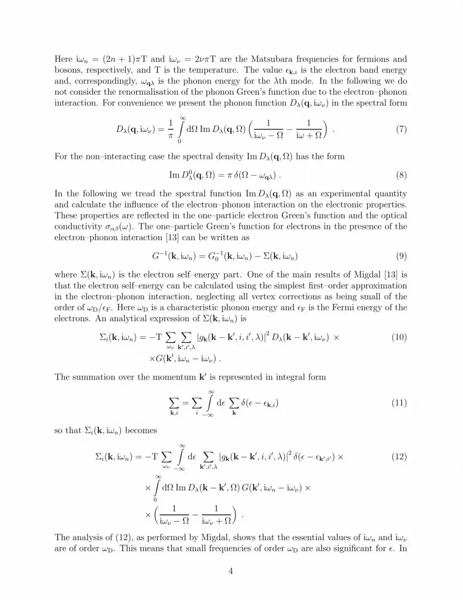
Firstly, we shall check the accuracy of the approximation of the expression (67) for σ(ω)by the “extended” Drude formula, Eq. (68). For that purpose we use the transport spectralfunction α2

tr(ω)F (ω) of the form shown in Fig. 1. A comparison between Eqs. (67) and (68)is shown in Fig. 2 for constants of coupling λtr = 1, where

λtr = 2

∞∫

0

dΩ

Ωα2

tr(Ω)F (Ω) . (72)

There are some differences in the low energy regime, ω <∼ 200 cm−1, shown in Fig. 3, especially

at low temperatures. One should be careful using the “extended” Drude formula in thiscase. However, even in this region the difference is rather small. The difference betweenthe conductivity calculated by the formulae (67) and (68) continues to be small even for aconstant of coupling λ ≃ 2.

The transport relaxation rate

1

τ ∗tr(ω)

=1

τtr(ω)

m

m∗(ω)(73)

13

has a universal behaviour for metals with different values of λ and different phonon density ofstates. Figure 4 shows the frequency dependence of the relaxation rate 1

τ∗

tr(ω)in dimensionless

form. Here ωm is the value of the maximum phonon frequency (i. e. the end of the phononspectrum). The six different curves plotted in Fig. 4 are indistinguishable as function of thedimensionless energy ω/ωm. The quantity 1

τ∗

tr(ω)is also rather universal as a function of the

dimensionless temperature T/πωm. Figure 5 shows 1τ∗

tr(ω)for T = 10 K and 100 K. Firstly, we

would like to emphasise the quasi–linear ω–dependence of 1τ∗

tr(ω)over a large energy interval,

0.5 ≤ ω ≤ (3− 4) ωm. The function 1τ∗

tr(ω)increases with increasing energy ω up to very high

values, ω ≃ 10 ωm. This contrasts strongly with the behaviour of the one–particle relaxationrate 1

τ(ω)defined by Eq. (31) and shown in the inset of Fig. 5. It is well known [17] that the

latter rapidly increases with energy and becomes constant for ω ≥ ωm. This difference inthe behaviour of the functions 1

τ∗

tr(ω)and 1

τ(ω)was first discussed in Ref. [6].

As mentioned above, there are only a few investigations [4,5] of the influence of theelectron–phonon interaction on the optical spectra of normal state metals where the fre-quency dependence of these effects was observed. Besides the reasons mentioned abovethere is another very important reason for the small number of such investigations. Namely,the absolute values of the frequency dependence of the discussed effects is determined bythe value of 1

τ∗

tr(ω)at ω →∞ [6]. This function can be written as

limω→∞

1

τ ∗tr(ω)

= πλ 〈ω〉 , (74)

where

λ 〈ω〉 = 2

∞∫

0

dω α2tr(ω)F (ω) . (75)

This value can be expressed as

1

τ ∗tr

≃ (1− 2) λωm , (76)

as can be seen from Figs. 4 and 5, and it is very small for ordinary metals. In lead, forexample, one finds λ 〈ω〉 ≈ 100 cm−1. It is extremely difficult to observe this phenomenain the usual reflection spectra. Therefore, the observation of Holstein processes in lead wasmade [4,5] using the light scattering inside a cavity whose walls hold the sample material.It was averaged over at least 100 such reflections to increase the accuracy of the experi-ment. It was shown [7,18] that a far–infrared measurement at low temperature, containingphonon–induced structure, can be inverted to give the spectral function of the electron–phonon interaction α2

tr(ω)F (ω). This function was obtained in Ref. [18] for lead in verygood agreement with experimental data from tunnelling measurements. We shall come backto discuss this observation in some more detail.

III. ELECTRON–PHONON INTERACTION AND OPTICAL SPECTRA OF

HTSC SYSTEMS

A large amount of work has been devoted to the study of optical spectra of HTSC systems(see for example the reviews [19,20]). Investigations include normal and superconducting

14

state properties, doping dependence, the effect of impurities, etc. . Here, we shall restrictour analysis to optimally doped HTSC in the normal state. In this case the optical spectraof all HTSC materials show quite similar behaviour: their reflectivity drops nearly linearlywith energy from R ≃ 1 down to R ≃ 0.1 at the plasma edge ω∗

p, where the values of ω∗p

vary for different HTSC materials, 1 eV ≤ ω∗p ≤ 1.8 eV [20]. Measurements for different

HTSC compounds further coincide in showing large values for the conductivity in the energyinterval 2 eV < ω < 15 eV and well developed charge fluctuation spectra (described by the

energy loss function −Im(

1ǫ(ω)

)

) in the energy interval 5 eV < ω < 40 eV [21]. The highenergy part of spectra above a few eV can be well described in terms of the usual bandstructure calculations [20,22]. Moreover, the calculations [22,23] can also describe quiteaccurately some low energy interband transitions in YBa2Cu3O7 [24].

The most unusual part of the optical spectra of HTSC systems is connected with thestrong decrease in reflectivity, almost linear in energy, in the region 0 ≤ ω ≤ ω∗

p ≃ 1 eV [25].This behaviour certainly cannot be explained with the simple Drude approach. Thomaset al [26] proposed two different ways of analysing such spectra. First, a one–componentFermi–liquid approach, using the “extended” Drude formula with frequency dependent massm∗(ω) and relaxation rate 1

τ(ω). This model successfully describes the heavy fermion sys-

tems [27]. Secondly, a two–component approach, where the spectrum is decomposed in twocomponents, the Drude part and a mid–infrared (MIR) absorption band. In the latter casethere is no unique way of separating the two components.

As we have discussed above, including the electron–phonon interaction in the consid-eration leads immediately to the representation of the optical conductivity in terms of the“extended” Drude formula. It has been shown earlier for some HTSC [6,8] that the existenceof strong electron–phonon coupling, including some amount of MIR excitations, can indeedexplain their optical conductivity. We now consider this approach in some more detail. Todescribe the optical spectra of HTSC systems we use the formulae obtained in section IIusing a transport spectral function α2

tr(ω)F (ω) of the form shown in Fig. 1, multiplied by ω2.This spectral function extends up to ωm = 735 cm−1 and well resembles the phonon spectraof HTSC systems. Generally, the optical properties do not depend on the actual shapeof α2

tr(ω)F (ω) but on some moments of it. Thus, we use the constant of electron–phononcoupling λtr as defined in Eq. (72) as fit parameter.

Figure 6 shows the reflectivity of optimally doped La2−xSrxCuO4 (LSCO) at room tem-perature. We have used the values ωp = 1.8 eV and ǫ∞ = 4.6 obtained by one of us [28] fromband structure calculations. The contribution of the electron–phonon coupling was supposedto be λtr = 2.5. The resulting reflectivity corresponds well to measurements on good qualityfilms [25]. The conductivity calculated in Ref. [28] describes well the optical spectra of LSCOat energies above ≈ 3 eV, as was confirmed by experiment [29]. Taking all this into account,we can conclude that the band structure approach joined with strong electron–phonon in-teraction can explain the overall behaviour of the optical spectrum of LSCO in the energyrange 0 < ω ≤ 40 eV. Moreover, this approach also explains the temperature dependenceof the optical spectrum of LSCO quite well. Figure 7 shows the reflectivity of LSCO in theFIR at temperatures T = 100, 200, 300 K. The agreement between experimental [30] andcalculated curves is good considering that the only fit parameter used was the constant ofcoupling λtr. In Fig. 8 we show the reflectivity for LSCO up to ω ≈ 1 eV for the sametemperatures. The agreement between calculated and measured curves is still quite good on

15

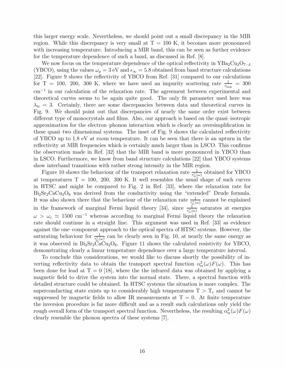
this larger energy scale. Nevertheless, we should point out a small discrepancy in the MIRregion. While this discrepancy is very small at T = 100 K, it becomes more pronouncedwith increasing temperature. Introducing a MIR band, this can be seen as further evidencefor the temperature dependence of such a band, as discussed in Ref. [8].

We now focus on the temperature dependence of the optical reflectivity in YBa2Cu3O7−δ

(YBCO), using the values ωp = 3 eV and ǫ∞ = 5.8 obtained from band structure calculations[22]. Figure 9 shows the reflectivity of YBCO from Ref. [31] compared to our calculationsfor T = 100, 200, 300 K, where we have used an impurity scattering rate 1

τimp= 300

cm−1 in our calculation of the relaxation rate. The agreement between experimental andtheoretical curves seems to be again quite good. The only fit parameter used here wasλtr = 3. Certainly, there are some discrepancies between data and theoretical curves inFig. 9. We should point out that discrepancies of nearly the same order exist betweendifferent type of monocrystals and films. Also, our approach is based on the quasi–isotropicapproximation for the electron–phonon interaction which is clearly an oversimplification inthese quasi–two dimensional systems. The inset of Fig. 9 shows the calculated reflectivityof YBCO up to 1.8 eV at room temperature. It can be seen that there is an upturn in thereflectivity at MIR frequencies which is certainly much larger than in LSCO. This confirmsthe observation made in Ref. [32] that the MIR band is more pronounced in YBCO thanin LSCO. Furthermore, we know from band structure calculations [22] that YBCO systemsshow interband transitions with rather strong intensity in the MIR region.

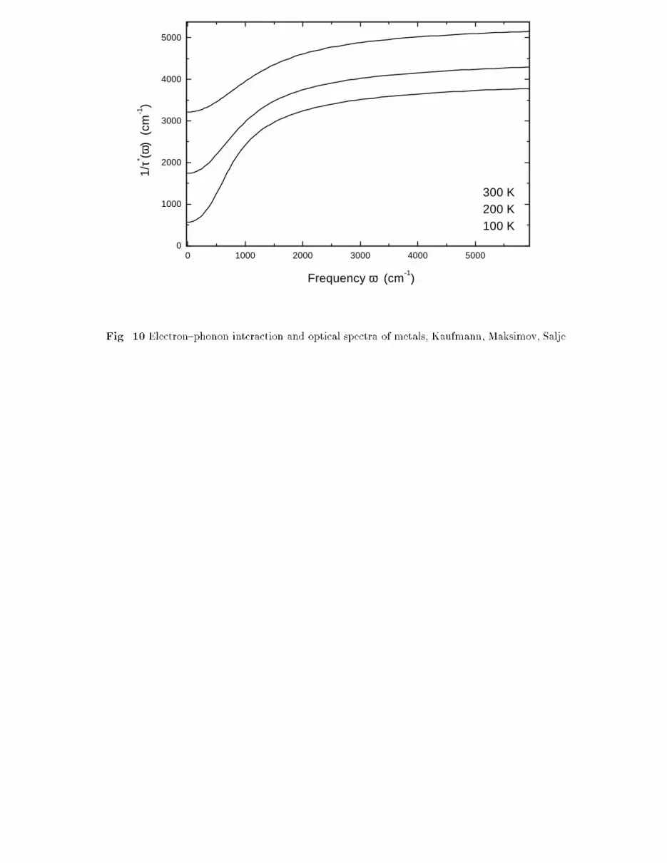
Figure 10 shows the behaviour of the transport relaxation rate 1τ∗

tr(ω)obtained for YBCO

at temperatures T = 100, 200, 300 K. It well resembles the usual shape of such curvesin HTSC and might be compared to Fig. 2 in Ref. [33], where the relaxation rate forBi2Sr2CaCu2O8 was derived from the conductivity using the “extended” Drude formula.It was also shown there that the behaviour of the relaxation rate 1

τ∗

tr(ω)cannot be explained

in the framework of marginal Fermi liquid theory [34], since 1τ∗

tr(ω)

saturates at energies

ω > ωc ≃ 1500 cm−1 whereas according to marginal Fermi liquid theory the relaxationrate should continue in a straight line. This argument was used in Ref. [33] as evidenceagainst the one–component approach to the optical spectra of HTSC systems. However, thesaturating behaviour for 1

τ∗

tr(ω)can be clearly seen in Fig. 10, at nearly the same energy as

it was observed in Bi2Sr2CaCu2O8. Figure 11 shows the calculated resistivity for YBCO,demonstrating clearly a linear temperature dependence over a large temperature interval.

To conclude this considerations, we would like to discuss shortly the possibility of in-verting reflectivity data to obtain the transport spectral function α2

tr(ω)F (ω). This hasbeen done for lead at T = 0 [18], where the the infrared data was obtained by applying amagnetic field to drive the system into the normal state. There, a spectral function withdetailed structure could be obtained. In HTSC systems the situation is more complex. Thesuperconducting state exists up to considerably high temperatures T > Tc and cannot besuppressed by magnetic fields to allow IR measurements at T = 0. At finite temperaturethe inversion procedure is far more difficult and as a result such calculations only yield therough overall form of the transport spectral function. Nevertheless, the resulting α2

tr(ω)F (ω)clearly resemble the phonon spectra of these systems [7].

16

IV. CONCLUSION

The results obtained in this work demonstrate clearly, that strong electron–phonon in-teraction, combined with band structure calculations, describe the overall behaviour of theoptical spectra and the main part of the transport properties of HTSC in a straightforwardmanner. However, we do not claim that this simple quasi–isotropic approach can explainall details of the behaviour of HTSC systems, even in the normal state, and even at optimaldoping. There are a number of open problems concerning the behaviour of the Hall coeffi-cient, the NMR relaxation rate of the copper sites. We would like to point out the existenceof at least two relaxation rates in the HTSC systems, namely the quasi–particle relaxationrate 1

τ(ω)and the transport 1

τ∗

tr(ω)which are very different over a large energy range. We

cannot rule out that the relaxation rate involved in the Hall current, due to strong and pos-sibly anisotropic electron–phonon interaction, will be different from the transport relaxationrate in those systems. This could lead to the observed temperature dependence of the Hallcoefficient.

Last but not least, we should point out that the simple approach presented here does notwork at low temperatures. It cannot properly describe the anisotropy of the superconductingorder parameter, although it yields the correct order of magnitude for the value of Tc. Thereare additional phenomena besides electron–phonon coupling which become important at lowtemperatures. There are a number of different models which combine a strong electron–phonon interaction with interband Coulomb interaction, with the existence of a Van Hovesingularity in the electron spectrum, etc., of which a detailed discussion is beyond the scopeof this work.

ACKNOWLEDGEMENT

The authors would like to thank O. Dolgov for many helpful discussions. They are alsograteful to S. Shulga for providing his program for this calculations. E. G. M. would like tothank the Royal Society and the Department of Earth Sciences, University of Cambridge,for their support and kind hospitality during his visit to Cambridge. He also acknowledgesthe RFBI for the financial support during the early stages of this work.

17

REFERENCES

[1] T. Holstein, Ann. Phys. (N.Y.) 29, 410, (1969)[2] P. B. Allen, Phys. Rev. B 3, 305 (1971)[3] G. B. Motulevich Sov. Phys. Uspekhi

[4] R. R. Joyce and P. L. Richards, Phys. Rev. Let. 24, 1007 (1970)[5] J. G. Bednorz and K. A. Muller, Z. Phys. B 64, 189 (1986)[6] S. V. Shulga, O. V. Dolgov, E. G. Maksimov, Physica C 178, 226 (1991)[7] O. V. Dolgov, S. V. Shulga, J. Supercond. 6, 611 (1995)[8] O. V. Dolgov, H. J. Kaufmann, E. K. H. Salje, and Y. Yagil Physica C 279, 113 (1997)[9] P. B. Allen, in Dynamical Properties of Solids, G. K. Horton, A. A. Maradudin, eds.

(Amsterdam, North Holland, 1980), Vol. 3, pp. 95[10] E. G. Maksimov, D. Yu Savrasov, and S. Yu Savrasov, Physics — Uspekhi 40, 337

(1997)[11] D. Rainer, in Progress in Low–Temperature Physics, D. F. Brewer, eds. (Amsterdam,

Elsevier, 1986), pp. 371[12] A. A. Abrikosov, L. P. Gor’kov, and I. E. Dzyaloshinski, Methods of Quantum Field

Theory in Statistical Physics, (Dover, New York, 1963)[13] A. B. Migdal, Sov. Phys. — JETP 39, 996 (1958)[14] P. B. Allen, Phys. Rev. B 13, 1416 (1976)[15] W. Lee, D. Rainer, and W. Zimmerman, Physica C 159, 535 (1989)[16] G. M. Eliashberg, Sov. Phys. — JETP 41, 1241 (1961)[17] P. B. Allen, B. Mitrovich, in Solid State Physics, M. Ehrenreich, F. Seitz, D. Turnball,

eds. (Academic Press, New York, 1982) Vol. 37[18] B. Farworth, T. Timusk, Phys. Rev. B 14, 5115 (1976)[19] D. B. Tanner, T. Timusk, in Properties of High Temperature Superconductors, D. M.

Ginsberg, ed. (World Scientific, Singapore, 1992) Vol. 3, pp. 363[20] S. Tajima, Superconductivity Review 2, 125 (1997)[21] N. Nucker, J. Fink, B. Renker, D. Everet, C. Politis, D. J. W. Weis, J. C. Fussle, Z.

Phys. B 67, 9 (1987)[22] E. G. Maksimov, S. N. Rashkeev, S. Yu Savrasov, and Y. A. Uspenskii, Phys. rev. Let.

13, 1880 (1989); Sov. Phys. — JETP 70, 952 (1990)[23] I. I. Mazin, D. Jepsen, O. K. Anderson, A. I. Leichtenstein, S. N. Reshkeev, Y. A.

Uspenskii, Phys. Rev. B 45, 5103 (1992)[24] B. Bucher, J. Karpinski, E. Kaldis, P. Wachter, Phys. Rev. B 45, 3026 (1992)[25] I. Bozovic, J. H. Klein, J. J. Harris Jr. E. S. Hellman, E. H. Hartferd, P. K. Chan, Phys.

Rev. B 46, 1182 (1992)[26] G. A. Thomas, J. Orenstein, D. H. Rapkine, D. H. Capizzi, A. J. Millis, R. N. Bhatt,

L. F. Schneemeyer, J. V. Waszczak Phys. Rev. Let. 61, 1313 1988[27] B. C. Webb, A. J. Sievers, T. Milalisin, Phys. Rev. Let. 57 1951 (1986)[28] I. I. Mazin, E. G. Maksimov, S. N. Rashkeev, S. Yu Savrasov, Y. A. Uspenskii, JETP

Letters 47, 113 (1988)[29] S. Uchida, K. Tamasaku, S. Tajima, Phys. Rev. B 53, 14558 (1996)[30] F. Gao, D. B. Romero, and D. B. Tanner, Phys. Rev. B 47, 1036 (1993)[31] J. Schutzmann, B. Gorshunov, K. F. Renk, J. Munzel, A. Zibold, H. P. Geserich, A.

Erb, G. Muller–Vogt, Phys. Rev. B 46, 512 (1992)

18

[32] Y. Yagil, F. Baudenbacher, M. Zhang, J. R. Birch, H. Kinder, E. K. H. Salje, Phys.

Rev. B 52, 15582 (1995)[33] D. B. Romero, C. D. Porter, D. B. Tanner, L. Forro, D. Mandrus, L. Mihaly, G. L.

Carr, G. P. Williams, Solid State Comm. 82, 183 (1992)[34] C. M. Varma, P. B. Littlewood, S. Schmitt–Rink, E. Abrahams, and A. E. Ruckenstein,

Phys. Rev. Lett. 63, 1996 (1989)

19

FIGURES

FIG. 1. Transport spectral function α2tr(ω)F (ω) used in the calculations.

FIG. 2. Comparison between the calculated optical conductivity (real part) σ1(ω) using Eq.

(67) (dashed line) and using the “extended” Drude formula, Eq. (68) (solid line).

FIG. 3. Same as Fig. 2 at low energies

FIG. 4. Transport relaxation rate 1τ∗

tr(ω) at T = 10 K for different constants of coupling,

λtr = 0.2, 0.6, 1.0, 1.4, and different phonon spectra with ωm = 612 cm−1, 735 cm−1, 882

cm−1, calculated using the “extended” Drude formula. In dimensionless units all curves fall on top

of each other.

FIG. 5. Transport relaxation rate 1τ∗

tr(ω) at T = 10 K and 100 K for λ = 1, ωm = 735 cm−1.

The inset shows the one–particle relaxation rate calculated for the same parameters.

FIG. 6. Calculated reflectivity for optimally doped LSCO at T = 300 K, using the “extended”

Drude formula with λ = 2.5, ωp = 1.8 eV, ǫ∞ = 4.6, 1/τimp = 100 cm−1.

FIG. 7. FIR reflectivity for LSCO from Gao et al at different temperatures compared to our

calculations.

FIG. 8. Same as Fig. 7 on a larger energy scale.

FIG. 9. FIR reflectivity for YBCO from Schutzmann et al at different temperatures compared

to our calculations, using λ = 3, ωp = 3 eV, ǫ∞ = 5.8, 1/τimp = 300 cm−1. The inset shows the

calculated curve at room temperature in a larger energy scale.

FIG. 10. Calculated transport relaxation rate 1τ∗

tr(ω) for YBCO at different temperatures.

FIG. 11. Calculated DC resistivity for YBCO as a function of temperature.

20

0 200 400 600 8000.0

0.2

α tr

2 ( ω)F

( ω)

Frequency ω (cm-1)Fig. 1 Electronphonon interaction and optical spectra of metals, Kaufmann, Maksimov, Salje

0 200 400 600 800 10000

10

20

30

40

50

100 K200 K300 K

σ 1(ω

) (

a.

u.)

Frequency ω (cm-1

)Fig. 2 Electronphonon interaction and optical spectra of metals, Kaufmann, Maksimov, Salje

0 100 2000

20

40

60

100 K200 K300 K

σ 1(ω

) (

a.

u.)

Frequency ω (cm -1)Fig. 3 Electronphonon interaction and optical spectra of metals, Kaufmann, Maksimov, Salje

0 2 4 6 80.0

0.2

0.4

0.6

0.8

1.0

10 K

1/τ* / λ

ωm

ω/ωmFig. 4 Electronphonon interaction and optical spectra of metals, Kaufmann, Maksimov, Salje

0 1 2 3 4 50.0

0.5

1.0 100 K 10 K

1/τ* / λ

ωm

ω/ωm

0.0 0.5 1.0 1.5 2.0 2.50.0

0.2

0.4

0.6

0.8

1.0

1.2

100 K 10 K

1/τ(

ω)/

ωm

ω/ωmFig. 5 Electronphonon interaction and optical spectra of metals, Kaufmann, Maksimov, Salje

0 2000 4000 6000 8000 10000 120000.0

0.2

0.4

0.6

0.8

1.0

300 K

Re

flect

ivity

R

Frequency ω (cm -1)Fig. 6 Electronphonon interaction and optical spectra of metals, Kaufmann, Maksimov, Salje

0 500 1000 1500 2000

0.7

0.8

0.9

1.0

100 K200 K300 K

Re

flect

ivity

R

Frequency ω (cm -1)Fig. 7 Electronphonon interaction and optical spectra of metals, Kaufmann, Maksimov, Salje

0 2000 4000 6000 8000

0.0

0.2

0.4

0.6

0.8

1.0

100 K200 K300 K

Re

flect

an

ce R

Frequency ω (cm -1)Fig. 8 Electronphonon interaction and optical spectra of metals, Kaufmann, Maksimov, Salje

0 5000 10000 15000

0.0

0.2

0.4

0.6

0.8

1.0

300 K

0 500 1000

0.85

0.90

0.95

1.00

100 K200 K300 K

Re

flect

an

ce R

Frequency ω (cm-1)Fig. 9 Electronphonon interaction and optical spectra of metals, Kaufmann, Maksimov, Salje

0 1000 2000 3000 4000 50000

1000

2000

3000

4000

5000

300 K200 K100 K

1/τ* ( ω

) (

cm-1)

Frequency ω (cm-1)Fig. 10 Electronphonon interaction and optical spectra of metals, Kaufmann, Maksimov, Salje

100 200 300 4000

20

40

60

80

100

120

140

Res

istiv

ity ρ

DC (

µΩcm

)

Temperature T (K)Fig. 11 Electronphonon interaction and optical spectra of metals, Kaufmann, Maksimov, Salje