arX

iv:0

804.

3509

v5 [

hep-

ex]

7 J

un 2

009

Electroproduction of η Mesons in the S11(1535) Resonance Region at High Momentum

Transfer

M.M. Dalton,1, ∗ G.S. Adams,2 A. Ahmidouch,3 T. Angelescu,4 J. Arrington,5 R. Asaturyan,6, †

O.K. Baker,7, 8 N. Benmouna,9 C. Bertoncini,10 W.U. Boeglin,11 P.E. Bosted,8 H. Breuer,12

M.E. Christy,7 S.H. Connell,13 Y. Cui,14 S. Danagoulian,3 D. Day,15 T. Dodario,14 J.A. Dunne,16

D. Dutta,16 N. El Khayari,14 R. Ent,8 H.C. Fenker,8 V.V. Frolov,17 L. Gan,18 D. Gaskell,8 K. Hafidi,5

W. Hinton,7, 8 R.J. Holt,5 T. Horn,12 G.M. Huber,19 E. Hungerford,14 X. Jiang,20 M.K. Jones,8

K. Joo,21 N. Kalantarians,14 J.J. Kelly,12, † C.E. Keppel,7, 8 V. Kubarovsky,8,2 Y. Li,7 Y. Liang,22

S. Malace,4 P. Markowitz,11 P. McKee,15 D.G. Meekins,8 H. Mkrtchyan,6 B. Moziak,2 T. Navasardyan,6

G. Niculescu,15 I. Niculescu,23 A.K. Opper,22 T. Ostapenko,24 P.E. Reimer,5 J. Reinhold,11 J. Roche,8

S.E. Rock,25 E. Schulte,5 E. Segbefia,7 C. Smith,15 G.R. Smith,8 P. Stoler,2 V. Tadevosyan,6 L. Tang,7, 8

V. Tvaskis,26 M. Ungaro,21 A. Uzzle,7 S. Vidakovic,19 A. Villano,2 W.F. Vulcan,8 M. Wang,25 G. Warren,8

F.R. Wesselmann,15 B. Wojtsekhowski,8 S.A. Wood,8 C. Xu,19 L. Yuan,7 X. Zheng,5 and H. Zhu15

1University of the Witwatersrand, Johannesburg, South Africa2Rensselaer Polytechnic Institute, Troy, New York 12180

3North Carolina A & T State University, Greensboro, North Carolina 274114Bucharest University, Bucharest, Romania

5Argonne National Laboratory, Argonne, Illinois 604396Yerevan Physics Institute, Yerevan, Armenia

7Hampton University, Hampton, Virginia 236688Thomas Jefferson National Accelerator Facility, Newport News, Virginia 23606

9The George Washington University, Washington, D.C. 2005210Vassar College, Poughkeepsie, New York 12604

11Florida International University, University Park, Florida 3319912University of Maryland, College Park, Maryland 2074213University of Johannesburg, Johannesburg, South Africa

14University of Houston, Houston, TX 7720415University of Virginia, Charlottesville, Virginia 22901

16Mississippi State University, Mississippi State, Mississippi 3976217LIGO Livingston Observatory, Livingston, LA 70754

18University of North Carolina Wilmington, Wilmington, North Carolina 2840319University of Regina, Regina, Saskatchewan, Canada, S4S 0A2

20Rutgers, The State University of New Jersey, Piscataway, New Jersey, 0885521University of Connecticut, Storrs, Connecticut 06269

22Ohio University, Athens, Ohio 4507123James Madison University, Harrisonburg, Virginia 22807

24Gettysburg College, Gettysburg, Pennsylvania 1810325University of Massachusetts Amherst, Amherst, Massachusetts 01003

26Nationaal Instituut voor Subatomaire Fysica, Amsterdam, The Netherlands(Dated: June 7, 2009)

The differential cross-section for the process p(e, e′p)η has been measured at Q2 ∼ 5.7 and 7.0(GeV/c)2 for centre-of-mass energies from threshold to 1.8 GeV, encompassing the S11(1535) reso-nance, which dominates the channel. This is the highest momentum transfer measurement of thisexclusive process to date. The helicity-conserving transition amplitude A1/2, for the production of

the S11(1535) resonance, is extracted from the data. Within the limited Q2 now measured, thisquantity appears to begin scaling as Q−3—a predicted, but not definitive, signal of the dominanceof perturbative QCD, at Q2 ∼ 5 (GeV/c)2.

PACS numbers: 14.20.Gk,13.60.Le,13.40.Gp,25.30.Rw

∗Electronic address: dalton@jlab.org†Deceased

I. INTRODUCTION

The goal of strong interaction physics is to understandhadrons in terms of their fundamental constituents, thequarks and gluons. Although these constituents are de-scribed by Quantum Chromodynamics (QCD), and per-turbative methods work well where applicable, mostly

2

the complexity of the theory precludes a description ofhadrons in terms of QCD. Various techniques are used tomake progress, such as numerical simulation of QCD andhadron models with effective QCD degrees of freedom.In this sense, the role of experiment is to make measure-ments which test the predictions of QCD-inspired quarkmodels. Most models can describe the static nucleonproperties and the baryon spectrum, and so other mea-surements, such as electromagnetic transition form fac-tors and strong decay amplitudes, are required.

A baryon’s quark substructure can be excited intoa resonance—an excited state of the quarks with well-defined baryon quantum numbers. The transition formfactor is the coupling (amplitude for the transition) fromone baryon state to another, as a function of the squaredinvariant momentum transferred to the baryon Q2. Themeasurements of couplings between baryon states andthe dependence of these on Q2, can be used as stringenttests of quark models. These couplings can be expressedin terms of the transition matrix elements between statesof definite helicity.

The difficulty in measuring baryon transition form fac-tors lies in isolating any of the multitude of wide and over-lapping resonant states. The S11(1535) is a baryon res-onance that can be accessed relatively easily. Althoughthere are many overlapping states in its mass region, itis very strongly excited over the accessible Q2 range andis the only resonance with a large branching fraction toη mesons [1], causing it to dominate the p(e, e′p)η chan-nel. This dominance is partly due to isospin conservation,since the proton has isospin= 1

2and the η has isospin=0,

only the N∗(I = 12) resonances can decay to a proton-η

final state—N∗(I = 32) resonances are forbidden.

As well as being accessible, the S11 is an interestingresonant state. It is the negative parity partner of thenucleon, they are both spin-half and isospin-half parti-cles. The transition form factor for the production ofthe S11 falls more slowly with Q2 than the dipole formfactor GD = (1 + Q2/0.71)−2, at least up to Q2 = 3.6GeV2 [2], and more slowly than the form factor for typ-ical baryons. An example is the D13(1520) [3], which isfrom the same SU(6)

⊗

O(3) multiplet and mass regionas the S11(1535). The S11(1535) branching fraction topη, at bη ∼ 50%, is anomalously high when compared tothat of the other N∗ resonances, a phenomenon which isnot well understood.

It is expected from helicity conservation in perturba-tive QCD (pQCD) that at sufficiently high Q2 the photo-coupling amplitude A1/2 will begin to scale as 1/Q3 [4],

or equivalently the quantity Q3A1/2 will flatten. The ob-servation of such scaling is thus a possible signal of thetransition to the dominance of hard processes. This mo-tivates the present experiment which studied exclusive ηproduction, allowing access to the amplitude A1/2 for the

S11 resonance, at the highest ever Q2 yet measured.The first measurement of η production at substantial

Q2 was published by Brasse et al. [5] in 1984 based onwork at DESY that went to Q2 = 2.0 and 3.0 GeV2.

This was the first indication that the S11(1535) falls farslower with Q2 than the D13(1520), and hence dominatesthe channel at high Q2.

In 1999, Armstrong et al. [2] published data obtainedin Hall C at Jefferson Lab at Q2 = 2.4 and 3.6 GeV2, thehighest until this work. The cross-section was found to beabout 30% lower than the DESY data and the full widthof the S11(1535) about twice as wide. By comparing withinclusive data, a lower bound was put on the branchingfraction S11 → ηp of bη > 0.45.

A recent paper by the CLAS collaboration from HallB at Jefferson Lab [6], published data for this process,at centre-of-mass (c.m.) energy W = 1.5 − 2.3 GeV andQ2 = 0.13 − 3.3 GeV2. The photocoupling amplitudeA1/2 of the proton to S11(1535) transition was extracted,and the anisotropies in the differential cross-section weremore precisely determined. The results for the magni-tude and width of the S11 resonance favoured the Arm-strong data over the older Brasse result. Evidence wasshown for a significant contribution to η electroproduc-tion due to a P -wave resonance with a mass around 1.7GeV.

This paper describes an experiment where electronswere scattered off free protons at high momentum trans-fer and both electron and proton were detected in co-incidence. In Sec. II the kinematics of the reaction arediscussed along with the formalities of the cross sectionand helicity amplitude for S11(1535) production. Sec. IIIdescribes the apparatus and methods used to acquire thedata. Sec. IV then goes on to present the processing ofthe data including corrections, calibration, cuts, MonteCarlo simulation, backgrounds and ultimately the crosssection extraction and error analysis. In Sec. V the η pro-duction differential cross section is plotted and fit withan angular dependence. A Breit-Wigner form is fitted tothe data and the S11 helicity amplitude and resonanceparameters are extracted. A brief summary is given inSec. VI. The appendix tabulates the extracted η produc-tion differential cross section.

II. FORMALISM

A. Kinematics

Figure 1 shows the one-photon exchange (Born) dia-gram for the resonance electroproduction process. Theincident electron ki scatters off the stationary protonpi with mass mp. We detect the scattered electron kf

and proton pf and reconstruct the undetected particle px

using the missing mass technique, evaluated from four-momentum conservation

m2x = (pi + ki − pf − kf )2. (1)

Using the symbols from the diagram and neglecting theelectron mass, the positive square of the four-momentum

3

q = (ν, ~q)

pi = (mp,~0)

ki = (E,~ki)

pf = (E′p, ~pf )

px = (Ex, ~px)

kf = (E′, ~kf )

1

FIG. 1: The one-photon exchange diagram of the resonanceelectroproduction process, where, for example, ki is the four-momentum vector of the incoming electron composed of en-

ergy E and momentum ~ki.

transferred from the lepton to hadron system is Q2 ≡−q2 = 4EE′sin2(θe/2). The mass of the resonant stateis W 2 = (q + pi)

2 = q2 + m2p + 2mpν.

Figure 2 shows the scattering and reaction plane coor-dinate systems: θe is the scattering angle of the electron;θpq the angle between the outgoing proton and the mo-mentum vector of the virtual photon, q; the polar andazimuthal angles of the missing momentum are θ∗x and φx

respectively, defined with respect to q and the electronscattering plane. A super-scripted * denotes measure-ment in the pη centre-of-momentum frame.

FIG. 2: The scattering and reaction plane coordinate systems.

B. Cross Section

The five-fold differential cross-section for the reactionmay be expressed as the product of the transverse virtualphoton flux ΓT and the centre-of-mass cross-section forthe electroproduction of the pη pair

d4σ

dWdQ2dφedΩ∗η

= ΓT (W, Q2)dσ

dΩ∗η

(γvp → pη), (2)

where the flux of transverse virtual photons in the Handconvention [7] is

ΓT (W, Q2) =α

4π2

W

mpE2

K

Q2

1

1 − ǫ, (3)

the longitudinal polarisation of the virtual photon isgiven by

ǫ =1

1 + 2 |q|2

Q2 tan2(θe/2), (4)

and the energy required by a real photon to excite aproton to a resonance of mass W is

K =W 2 − m2

p

2mp. (5)

The unpolarised virtual photon cross-section is writ-ten in terms of the transverse polarised virtual photondσT /dΩ∗

η, longitudinal polarised virtual photon dσL/dΩ∗η

and interference contributions, dσLT /dΩ∗η and dσTT /dΩ∗

η

in Eq. (6). Each of these four individual components areexpressed in terms of multipoles [8, 9], where El±, Ml±

and Sl± are the electric, magnetic and scalar multipolesrespectively; l is the orbital angular momentum, and ±indicates the total angular momentum via j = l ± 1

2. If

only terms with l ≤ 2 and either of the dominant isotropicmultipoles, E0+ or S0+, are retained, then Eqs. (7) areobtained [10].

The virtual photon cross-section is parametrised interms of its angular dependence as Eq. (8). The pa-rameters A−F are then given in terms of the truncatedmultipole expansion by the Eqs. (9).

dσ

dΩ∗η

(γvp → pη) =dσT

dΩ∗η

+ ǫdσL

dΩ∗η

+√

2ǫ(1 + ǫ)dσLT

dΩ∗η

cosφ∗η + ǫ

dσTT

dΩ∗η

cos2φ∗η (6)

dσT

dΩ∗η

=|p∗

η|WmpK

|E0+|2 − Re[

E∗0+

2cosθ∗ηM1− − (3cos2θ∗η − 1)(E2− − 3M2−)

]

;

dσL

dΩ∗η

=Q2

|q∗|2|p∗

η|WmpK

|S0+|2 + 2Re[

S∗0+

2cosθ∗ηS1− − 2(1 − 3cos2θ∗η)S2−

]

;

dσTL

dΩ∗η

=

√

Q2

|q∗|2|p∗

η|WmpK

− sinθ∗ηRe[

E∗0+(S1− + 6cosθ∗ηS2−) + S∗

0+

M1− + 3cosθ∗η(M2− − E2−)

]

;

4

dσTT

dΩ∗η

=|p∗

η|WmpK

− 3sinθ∗ηRe[

E∗0+(M2− + E2−)

]

; (7)

dσ

dΩ∗= A + B cosθ∗ + C cos2θ∗ + D sinθ∗cosφ∗ + E cosθ∗sinθ∗cosφ∗ + F sin2θ∗cos2φ∗ (8)

A =|p∗

η|WmpK

|E0+|2 + ǫQ2

|q∗|2 |S0+|2 −(

Re[

E∗0+(E2− − 3M2−)

]

+ 4ǫQ2

|q∗|2 Re[

S∗0+S2−

]

)

B =|p∗

η|WmpK

− 2Re[

E∗0+M1−

]

+ 2ǫQ2

|q∗|2 Re[

S∗0+S1−

]

C =|p∗

η|WmpK

3(

Re[

E∗0+(E2− − 3M2−)

]

+ 4ǫQ2

|q∗|2 Re[

S∗0+S2−

]

)

D =|p∗

η|WmpK

−√

2ǫ(ǫ + 1)

√

Q2

|q∗|2 Re[

E∗0+S1− + S∗

0+M1−

]

E =|p∗

η|WmpK

− 3√

2ǫ(ǫ + 1)

√

Q2

|q∗|2 Re[

2E∗0+S2− + S∗

0+(M2− − E2−)]

F =|p∗

η|WmpK

− 3ǫRe[

E∗0+(E2− + M2−)

]

(9)

C. Helicity Amplitude

The helicity amplitude is the matrix element that con-nects states of definite (the same or different) helicity. Assuch, it is a convenient measure of the coupling strengthbetween states and can be used to fundamentally testquark models. The amplitudes are labelled by the virtualphoton polarisation (either transverse A or longitudinalS) and the total γN helicity (1

2or 3

2). Spin- 1

2resonances

are therefore described only by A1/2 and S1/2.The helicity amplitude A1/2, for the process γvp →

S11(1535), can be obtained from the contribution of theS11(1535) to the E0+ multipole at the resonant massW = WR, using [11, 12]

A1/2 =

[

2π|p∗

η|RWR

mpK

WR

mp

ΓR

bη

]1/2

|E0+(WR)|. (10)

This requires, not only isolating the S11(1535) fromthe other resonances and the non-resonant background,but further isolating the E0+ multipole from the othermultipoles. In this case, for γvp → ηp at the S11(1535)resonance mass, such an isolation is almost implicit inthe measurement due to the dominance of the S11(1535).Being an S-wave resonance, implies a dominance of theisotropic multipoles—which has previously been seen inthe data [2, 5, 6, 13]. So too, among the isotropic con-tributions it appears that the transverse multipole E0+,dwarfs the longitudinal part S0+ [3, 6, 14].

Doing a longitudinal/transverse (LT ) separation re-quires measuring the cross-section for at least two values

of ǫ at the same Q2, which was not done in this exper-iment. Such separations performed in the late 1970’sare consistent with no longitudinal component. WhereR = σL/σT is the ratio of longitudinal to transversecross sections, Ref [14] found R = 0.23 ± 0.15 at Q2

= 0.4 GeV2 and Ref [3] found R = 0.22 ± 0.23 at Q2

= 0.6 GeV2 and R = -0.16 ± 0.16 at Q2 = 1 GeV2.Quark models [15] show this ratio decreasing with Q2.In angular fit to their recent data, Denizli [6] shows thatthe parameters of the P 1(cosθ∗η)cosφ components fluctu-ate around zero and are consistent with zero within ex-perimental uncertainty. These parameters measure thedσLT /dΩ component of dσ/dΩ, suggesting that the lon-gitudinal component is small—but since dσLT/dΩ∗ is asum of terms with possibly different signs, it is possiblethat S0+ is in fact comparable to E0+.

In this paper it is assumed that the longitudinal ampli-tudes are not significant for this reaction. The validity ofthis will become clear in the future when LT separationsare done at high Q2.

The cross-section can thus be written as dependingonly on the dominant E0+ multipole in the simple form

dσ

dΩ∗η

≈|p∗

η|WmpK

|E0+|2. (11)

The combination of Eq. (11) and Eq. (10) yields

A1/2(Q2) =

√

WRΓR

2mpbησR(Q2), (12)

the helicity amplitude as a function of σR ≡ σ(WR) [the

5

total cross-section of the S11(1535) resonance, measuredat the resonance mass WR.]

The E0+ multipole can be more reliably extracted froma fit to the angular dependence. Parameters A and C inEqs. (9) share some common terms, and a simple cancel-lation yields Eq. (13)—although in the absence of an LTseparation, it still must be assumed that S0+ is negligible.

A +1

3C =

|p∗η|W

mpK

|E0+|2 + ǫQ2

|q∗|2 |S0+|2

≈|p∗

η|WmpK

|E0+|2 (13)

Where possible in this work, the E0+ multipole is ex-tracted using both methods, but for consistency with pre-vious analyses the final result is quoted from the methodassuming isotropy.

III. THE EXPERIMENT

Cryogenictargets HMS

(protons)

SOS(electrons)

Beam

meters0 5 10

To BeamDump

Hall C

FIG. 3: A plan view of Hall C showing the beamline, targetand the SOS and HMS spectrometers which detected electronsand protons respectively. Figure from Ref. [2].

The experiment, measuring the unpolarised differentialcross-section for the process p(e, e′p)η, was performed inHall C (Fig. 3) of the Thomas Jefferson National Ac-celerator Facility, during May and June of 2003. TheShort Orbit Spectrometer (SOS) [16], a resistive QDD(quadrupole, dispersive dipole, anti-dispersive dipole)spectrometer, was used to detect scattered electrons. TheHigh Momentum Spectrometer (HMS) [17], with a su-perconducting QQQD configuration, detected the recoil

protons. The η particles were identified using the missingmass method.

Both spectrometers have a similar detector ensem-ble, including drift chambers for determining the track,scintillator arrays for triggering, an electromagneticcalorimeter for particle identification (PID) and a thresh-old gas Cerenkov also for PID and tuned to differentiatebetween pions and electrons in the SOS. Figure 4, show-ing the detector components, is representative of eitherdetector stack.

DC1

DC2S1X

S1Y

S2XS2Y

Pb-glassCalorimeter

x

zgas Cerenkov

FIG. 4: A side view of the HMS detector stack, which isalso representative of the SOS. The detected particles travelfrom left to right, encountering first the two drift chambers(DC) then the first two arrays of scintillators (S1) oriented inthe X and Y directions, then the gas Cerenkov detector, thethird and fourth scintillator arrays and finally the calorimeter.Figure from Ref. [2]

The Jefferson Laboratory’s superconducting radiofre-quency Continuous Electron Beam Accelerator Facility(CEBAF) provides multi-GeV continuous-wave beamsfor experiments at the nuclear and particle physics in-terface [18]. The accelerator consists of two anti-parallellinacs linked by nine recirculation beam lines in the shapeof a racetrack, for up to five passes. Beam energies up tonearly 6 GeV at 100 µA and > 75% polarization are pos-sible. For this experiment, the incident electrons had themaximum available energy: Ee = 5.500 GeV for most ofthe experiment and Ee = 5.491 GeV for an 11 day periodnear the beginning.

The target was liquid hydrogen maintained at a tem-perature of 19 K. The beam passes through 3.941 cmof liquid and through 0.12 mm of aluminium target cellwalls on entrance and exit. The beam was rastered withina square of ± 1 mm to minimise density changes due totarget boiling. A dummy target consisting of two alu-minium plates was used to simulate reactions within thetarget walls.

The trigger for the experiment was a coincidence be-tween pre-triggers (or singles triggers) from both of the

6

spectrometers. Both of the spectrometer pre-triggerswere the requirement of a signal in three out of the fourscintillator planes (SCIN). In addition to the coincidencetrigger, data were taken for singles triggers from both ofthe two spectrometers. This was pre-scaled according tothe rate so as not to interfere with the coincidence trigger.This singles data allowed the monitoring of the luminos-ity and the electron detection efficiency. The elastic scat-tering events within the SOS were used to monitor thebeam energy and the performance of the SOS magnets.

Blok et al. [19] is descriptive of the accelerator, beammonitoring equipment and current monitors, target ras-tering system, beam energy measurement and cryogenictarget. More detailed discussions are made of the twospectrometers, their detector packages, the trigger logicand data acquisition. Further references are provided forall covered topics, the interested reader is advised to con-sult that work.

The electron spectrometer was fixed in angle and mo-mentum, thereby defining a central three-momentumtransfer vector ~q for the virtual photon which mediatesthe reaction. Around this ~q vector is a cone of reac-tion products including the protons from the resonancedecay of interest in this measurement. The “kinematicfocusing” caused by the high momentum transfer of thereaction makes it possible to capture a large fraction ofcentre of mass decay solid angle in a spectrometer, as itcomes out as a “narrow” cone in the lab. The protonspectrometer was stepped in overlapping angle and mo-mentum steps to capture as much of this decay cone aspossible.

The exact choice of kinematics was based on a compro-mise between maximising the Q2 for the available beamenergy and detecting the full centre-of-mass decay conefor the p(e, e′p)π0 reaction to the highest possible W .This reaction, which was measured concurrently is re-ported on by Villano [20]. The maximum central mo-mentum of the SOS, 1.74 GeV, required increasing θSOS

to increase the Q2, while the minimum HMS angle of 10.5degrees required decreasing θSOS to extend the full angu-lar coverage to higher W . At θSOS = 47.5 degrees and themaximum SOS momentum, it was found that the kine-matic region from pion threshold to above the S11 massfell nicely within the best resolution region of the SOSspectrometer and full cosθ∗ coverage was possible for thepπ0 up to W = 1.4 GeV and pη up to W = 1.6 GeV,as shown in Fig. 5. These SOS central parameters cor-respond to a virtual photon with momentum 4.51 GeVand angle 16.5 degrees and Q2 ∼ 5.8 (GeV/c)2 at the S11

resonance mass.

In addition to data taken with these kinematics, it wasdecided to take a smaller set of data at even higher Q2,although the angular coverage would be incomplete. Inthis configuration the SOS was set with central momen-tum of 1.04 GeV and angle of 70 degrees, which givesa central virtual photon with |~q| = 5.24 GeV and angle10.8 degrees and Q2 ∼ 7.0 (GeV/c)2 at the S11 resonancemass. For the purposes of this paper, the first data set

FIG. 5: The W acceptance of the detector pair for thee(p, e′p)η reaction, in the lower-Q2 configuration, as a func-tion of the laboratory scattering angle and momentum of theproton. The contours are constant W of the hadronic sys-tem, for an electron at 47.5 degrees and momentum of 1.74GeV/c, for the full range of θ∗ and φ = 0 and 180 degrees.The solid central contour is W = 1.5 GeV, from which theyincrease in steps of 100 MeV to the outermost at W = 1.9GeV. In practice, the angle and momentum bite of the SOScauses the contours to be much broader. Each black box isthe acceptance of a particular HMS setting (†Table I). Thealternate settings are offset by 1.5 and are a 4.7% increasein momentum, so that they are approximately centred on thepoints where the boxes join.

will be called the ‘lower-Q2’ configuration and the seconddata set, the ‘higher-Q2’. The kinematic settings for theexperiment are summarised in Table I.

Electron Arm Proton ArmpSOS θSOS pHMS θHMS

GeV degrees GeV degrees

4.70 18.0, 15.04.50† 19.5, 16.5, 13.5, 11.23.90 21.0, 18.0, 15.0, 12.03.73† 22.5, 19.5, 16.5, 13.5, 11.2

1.74 47.5 3.24 24.0, 21.0, 18.0, 15.0, 12.03.10† 22.5, 19.5, 16.5, 13.5, 11.22.69 24.0, 21.0, 18.0, 15.0, 12.02.57† 22.5, 19.5, 16.5, 13.5, 11.22.23 21.0, 18.0, 15.0, 12.02.13† 22.5, 19.5, 16.5, 13.54.70 11.24.50 14.2

1.04 70.0 3.90 11.23.73 14.2, 11.23.24 11.2

TABLE I: The kinematic settings of the two spectrometers.

7

Data were taken at a mean beam current of 92 µA.The lower-Q2 configuration was run for 6 weeks, totaling127 C of electrons through the target from which about50,000 η particles were identified from proton-electroncoincidences, by missing mass reconstruction. Due toimproved accelerator operation, the one week of runningfor the higher-Q2 setting received 29 C of charge, butonly about 2,000 η particles were reconstructed.

IV. DATA ANALYSIS

The raw data as recorded by the electronics were re-played offline to produce PAW or root ntuples of cali-brated physics quantities. Corrections were made to thedata for inefficiencies, dead times and accidental coinci-dences. The detector response was simulated using theMonte Carlo technique (including multiple scattering inthe detector and nuclear reactions in the target walls)with one input model cross-section for the η productionsignal and another model for the multipion backgroundprocesses, described in detail in Sec. IVC. Using an it-erative procedure, a linear combination of the signal andbackground simulations was fitted to the data and theresult used to refine the simulation input model, untilthe simulation in each bin matched the data with a mul-tiplicative factor of close to unity.

A. Raw Data to Physical Quantities

The raw data from each trigger was stored onto tape.These data were “replayed” offline a number of times dur-ing the analysis, using the Hall C data reduction code, asthe calibration of the detectors was improved. For eachevent, a list of calibrated event properties including posi-tion and angles of the track, timing and energy depositioninformation were determined. So too were quantities forthe scattering including the centre-of-mass angles, invari-ant hadronic mass and the missing mass. For each runan ntuple of these event parameters was produced alongwith a file containing scaler information and calculatedefficiencies and dead times for that run.

The data were corrected on a run-by-run basis forthese inefficiencies and dead times during the fillingprocedure—each event passing the cuts was filled intothe histogram weighted by a run dependent correctionfactor. This included track reconstruction inefficienciesin the HMS and SOS spectrometers and computer andelectronic dead times. A summary of all the correctionsapplied to the data is given in Table II.

The pion form factor (Fπ) experiment [19, 21] was con-ducted in the same suite of experiments as the currentexperiment and this work makes reference to some analy-ses reported there. A detailed description of the fitting ofthe reconstruction matrix elements for the spectrometersis included there. A number of offsets and correctionswere determined by analysing singles elastic scattering

Effect lower-Q2 higher-Q2

Proton absorption +4 ± 1%†Computer DT +(1.0 − 19.1)% +(1.8 − 10.9)%†HMS tracking +(2.3 − 14.3)% +(3.3 − 7.4)%†SOS tracking +(0.3 − 0.9)% +(0.2 − 0.8)%†Electronics DT +(0.0 − 2.4)% +(0.0 − 0.6)%‡Random coincidence −(0.0 − 7.6)% −(0.0 − 1.2)%

TABLE II: Corrections applied to the data. For correctionsapplied †run-by-run or ‡bin-by-bin, the range of the size isindicated in parentheses.

and coincident 1H(e, e′p) events. From these kinemati-cally overdetermined reactions, it was possible to checkthe momentum p and angles θ and φ (in-plane and out-of-plane relative to the spectrometer central axis respec-tively) for both spectrometers, and the beam energy E.A fit was done to determine what offsets to these quanti-ties most accurately produced the required values for theinvariant hadronic mass, and missing mass and energyfor the elastic scattering. In the case of SOS momen-tum (equivalently the dipole field), there is a saturationas the current is increased due to the resistive nature ofthe magnets. A field dependent correction was thus de-termined. These offsets, summarised in Table III, wereused in the replay of the present data.

Quantity HMS SOSθ 0.0 ± 0.5 mrad 0.0 ± 0.5 mradφ +1.1 ± 0.5 mrad +3.2 ± 0.5 mradp (lower-Q2) −0.13 ± 0.05% −1.36 ± 0.05%p (higher-Q2) 0.00 ± 0.05%Ee 0.00 ± 0.05%

TABLE III: Nominal 2003 spectrometer offsets [19, 21] ap-plied to the data during the replay phase.

1. Trigger Efficiency

The HMS trigger was a three out of four coincidencebetween the four scintillator planes. A trigger inefficiencyfor proton detection in the HMS is produced by protonswhich are not detected in their interaction with the scin-tillator, and by protons that do not make it through allthe scintillators due to absorption.

A previous study of general HMS trigger efficiency [19,21] showed a strong dependence on relative particle mo-mentum δHMS. The momentum in the spectrometersis measured relative to the central momentum pset, sothat particles with the same δ = (p − pset)/pset are dis-persed by the same amount. The trigger efficiency wasmostly very high at 0.995 but dropped rapidly for mo-menta lower than δ ∼ −6%. The data was analysed with

8

a cut of δ > −6 resulting in an average increase in ex-tracted cross-section of 1.4%. No correction for this effectwas made, but this figure was used as an estimate of theerror due to the trigger efficiency.

The trigger requires hits in scintillator planes S1and S2, so another source of inefficiency is absorption,through nuclear reactions, of the proton in target or de-tector materials before the S2 plane. The total pp colli-sion cross-section, σpp, varies slightly from 47 to 42 mbfor proton lab momenta between 2 to 5 GeV/c [1] whichis the momentum range of this experiment. Therefore forthis experiment, the trigger efficiency due to absorptionis relatively independent of kinematic setting.

The primary sources of interacting material are the S1scintillator planes which had a thickness of 1 cm each andthe Aluminium windows of the gas Cerenkov and aerogeldetectors which had a total thickness of 0.51 cm. Theproton-nuclear cross-section was estimated as A0.7σpp.Combining interactions in all material, the trigger effi-ciency due to proton absorption is estimated to be 0.95.

To calculate the correction used in the experiment forthe trigger efficiency due to proton absorption, a studyof ep elastic events was done. The SOS was set for elec-trons at central angle = 50 and central momentum of1.74 GeV/c and the HMS was set for protons at centralangle of 18 and central momentum of 4.34 GeV/c at abeam energy of 5.247 GeV. For a point target, the SOShas an out-of-plane angular acceptance of ±37 mr andan in-plane angular acceptance of ±57 mr (the in andout-of-plane angles are relative to the central axis of thespectrometer), while the HMS has an out-of-plane angu-lar acceptance of ±70 mr and an in-plane angular accep-tance of ±27 mr. The ratio of electron to proton momen-tum is 0.4, so for the maximum SOS out-of-plane angle,the corresponding HMS out-of-plane angle is 15 mr. Themaximum SOS in-plane angle gives a corresponding HMSin-plane angle of 23 mr. The data acquisition is set-upto accept singles triggers from the SOS and HMS indi-vidually in addition to coincidence triggers between theHMS and SOS.

In offline analysis, the cuts described in Sec. IVB 1were used to identify electrons in the SOS. A good elasticevent in the SOS was identified by a cut of 0.9 < W <1.0 GeV and a cut on the SOS in-plane angle of ±50 mrwhich ensured that the proton would be within the HMSangular acceptance. The proton was selected by the time-of-flight between electron and the particle detected in theHMS. The raw number of coincident ep events was 2009and the number of single events was 205.

Some data were taken with an aluminium “dummy”target, which is intended to model an empty target cell,but is 7.78 times thicker in order to increase the countrate. Analysis of this data determined that the targetendcaps would contribute 12 ± 3 events to the raw co-incidence events and 123.0 ± 12 events to the raw singleevents. Therefore the proton trigger efficiency due toabsorption is 0.96 ± 0.01, in good agreement with theprediction. A 4% correction was applied to the data for

this effect.

2. Calibration of Simulation Resolution

As described in Section IVB3, the cross section is ob-tained by integrating over the η missing mass peak. Thesensitivity to the exact shape of the peak is thus smalland is minimised by matching the simulation resolutionto the data resolution as far as possible. This was donefor the elastic peak, following which the simulation of theeta peak was in agreement with the data width withoutfurther change.

The elastic scattering of electrons into the SOS andprotons into the HMS were compared to SIMC MonteCarlo simulations of the same. The invariant mass deter-mined from elastic scattering must be the proton mass,but is broadened due to resolution effects and radiativetails—which are included in the simulation. In both de-tectors it was found that the width of this peak predictedby the simulation was narrower than for the data. Theseresolution differences were taken into account by increas-ing the drift chamber resolutions in each spectrometer,from the nominal value of 300 µm. The resolution wasvaried, and the simulation repeated, until a Gaussian fit-ted to the simulated spectrum had the same width asa Gaussian (and polynomial background) fitted to thedata. It was found that the HMS needed a drift cham-ber resolution of 570 µm to match the data width of17.2 MeV, while in the SOS, the 30.1 MeV width wasachieved with a 350 µm resolution.

This method had the effect of degrading the optics ofthe simulation slightly to match the experimental trans-port matrix elements of the data, in a logical yet simplemanner. During the systematic error analysis process,described in Section IVF, the drift chamber resolutionswere varied by 10% and the integration limits were var-ied by 0.1 GeV2, characterising the sensitivity of the ex-tracted differential cross-sections and amplitudes.

3. Collimator Punch Through

A source of background is due to particles that interactwith the edges of the HMS collimator aperture, locatedjust before the first quadrupole magnet, whose kinemat-ics are thus changed. The collimator is made from 6.35cm thick HEAVYMET (machinable Tungsten with 10%CuNi; density=17 g/cm3.) For practical purposes elec-trons are stopped by the SOS collimator, but protonshave the possibility of “punching” through the collima-tor, undergoing multiple scattering and energy loss in thematerial, and still making it through the spectrometer tothe detectors. This process is modelled in the simulationof the experiment and additionally a loose cut, 3 cen-timeters outside the collimator edge, is used to eliminateunphysical reconstructions.

9

4. Data Cuts

The ‘standard’ cuts are listed in Table IV. The cutson relative electron momentum δSOS, and relative protonmomentum δHMS, are made to ensure that only parti-cles within the well understood region of the spectrom-eter momentum acceptance are used. The momentumin the spectrometers is measured relative to the cen-tral momentum pset, so that particles with the sameδ = (p − pset)/pset are dispersed by the same amount.

Some parts of the SOS spectrometer acceptance, dueto an ambiguity in the solution of the optics equations,do not reconstruct reliable tracks. The cuts on the SOSfocal plane position in the magnet dispersion direction,XSOS,f.p., are to eliminate these regions. The particleidentification cuts are described in Section IVB.

Quantity Variable CutElectron momentum δSOS < +20%

> −15%Proton momentum δHMS < +9%

> −9%SOS focal plane position XSOS,f.p. > −20 cm

dispersive direction < +22 cm†Coincidence time |tcoin − tcent| < 1.5 ns†SOS Cerenkov Np.e. > 0.5†SOS calorimeter Enorm > 0.7

TABLE IV: The set of ‘standard’ cuts applied to the data andto the simulations where applicable. †The Particle Identifica-tion cuts are not applied to the simulation.

5. Binning

The data were binned in W , cosθ∗η, φ∗η and m2

x, whereW is the invariant mass of the hadronic system, θ∗η isthe polar angle between the direction of the η and thethree-momentum transfer vector ~q in the centre-of-massof the resonance, φ∗

η is the azimuthal angle of the η with

respect to the electron scattering plane, and m2x is the

square of the missing mass for p(e, e′p)x.For the lower-Q2 data, this was done in 12 cosθ∗η-bins

and 8 φ∗η-bins, to maximise the angular resolution for

partial-wave analyses, necessitating m2x-bins of 0.1 GeV2

and W -bins of 30 MeV near the resonance and 40 MeV athigher W . The higher Q2 data, with far fewer detectedparticles, was binned with W -bins of 30 MeV, 6 cosθ∗η-

bins, 5 φ∗η-bins and m2

x-bins of 0.15 GeV2.Bins in (W , cosθ∗η, φ∗

η) were retained for the analysisif they passed the following three criteria. Firstly, in theregion of the η missing mass peak, the simulation was re-quired to predict a signal to background ratio of at least0.25. Secondly, the simulation needed to have predicteda minimum average number of η events in the peak of1.5 per missing mass squared channel. This criterion was

used instead of requiring a total number of predicted ηparticles because the resolution of the missing mass peakchanges substantially with cosθ∗η. The third criterion foracceptance was, following the subtraction of the all thebackgrounds, the sum of the data in the region of themissing mass peak was required to have a statistical un-certainty of less than 50%.

B. Particle Identification

1. Electron Identification

In the SOS spectrometer, the Cerenkov detector andthe electromagnetic calorimeter were used to identifyelectrons and reject pions. The Cerenkov detector wasfilled with Freon-13 at 1 atmosphere, yielding a veloc-ity threshold of βt = 1/n = 0.9992. The highest mo-menta detected by the SOS in this experiment was about2.09 GeV/c, corresponding to β = 0.9978 for pions, whichis below the threshold for detection while all electrons arewell above the threshold. Some pions make small signalsin the Cerenkov due to scintillation or “knock-on” elec-trons from atomic scattering. The detected signal wascalibrated into units of the number of photo-electrons,Np.e..

For each event, the signals from each of the 44 lead-glass blocks in the calorimeter were summed to obtain thetotal energy deposited, Etot. This energy was then nor-malised by the momentum of the particle as determinedby the tracking, ptrack, to obtain Enorm = Etot/ptrack.The 16 radiation lengths of lead-glass bring electrons toa stop, resulting in a peak at Enorm ∼ 1 due to elec-trons. The pions peak at about Enorm ∼ 0.25, but havea long tail to higher Enorm due to the charge exchangenuclear interaction π−p → π0nx, and subsequent decayπ0 → γγ.

Figure 6 shows the correlation between Enorm and Np.e.

for the lower-Q2 data. The electrons are clearly well sep-arated from the pions by these two detectors. In theanalysis, electrons are identified using two simple cuts,Np.e. > 0.5 and Enorm > 0.7, shown in the figure.

2. Proton Identification and Accidental CoincidenceSubtraction

Protons were separated from pions using time of flightconsiderations. The raw difference in arrival times, tdiff ,between the electron in the SOS and the positive particlein the HMS, were corrected event-by-event for differencesin path length of both particles through the detectorsand the variation in velocity β of the positive particle(all electrons having essentially the same velocity.) Thiscorrected coincidence time, tcoin, is plotted in Fig. 7 andshows peaks due to protons and π+ particles and a back-ground of accidental (or random) coincidences.

10

p.e.Cerenkov N0 5 10 15 20 25

norm

Cal

orim

eter

E

0

0.2

0.4

0.6

0.8

1

1.2

1

10

210

310

410

510−e

−π

FIG. 6: The correlation between Enorm and Np.e. for allthe lower-Q2 data. The particle ID cuts to select electrons,Np.e. > 0.5 and Enorm > 0.7, are visible as dashed lines inthe figure. All other cuts listed in Table IV have already beenapplied to the data.

The path taken is determined by the tracking algo-rithm from drift chamber hit positions while the velocityβ = (p2/(m2

p + p2))1/2 is calculated from the measuredmomentum p assuming the proton mass mp. For pro-tons the corrected coincidence time depends only on theactual difference in starting times of the particles in thetarget, causing a peak of real coincidences, which hasbeen shifted to zero in the figure. Particles with a dif-ferent mass, such as pions, have their coincidence timepeak shifted relative to the protons since for the samemomentum, they have a different velocity. The π+ peakis broader than the proton peak because tcoin is calcu-lated to remove the momentum dependence of the pro-tons but the pion locus remains momentum dependent.A much smaller number of kaons are detected and forma locus between the pions and protons, but remain dis-tinctly separable. It was then possible to select the pro-ton events and reject the pion and kaon events and mostof the accidental coincidences using one simple cut.

Accidental coincidences occur when both detectors aretriggered within the 100 ns coincidence time window,but the detected particles originate in different scatter-ing events. In the coincidence time spectrum of Fig. 7,the accidentals are the continuous background under thetwo main peaks. The 2 ns beam structure can clearly beseen in the spectrum. A 3 ns particle identification win-dow was used to select protons, but within this cut thereis still some background due to accidental coincidenceswhich must be subtracted.

For each bin in 4 dimensions (W , cosθ∗η, φ∗η and m2

x),the number of accidental coincidences inside the protoncut was estimated by determining the average numberof accidentals in the “wings” of the spectrum, −45 ns <tcoin < −5 ns and 15 ns < tcoin < 50 ns, away from locifor actual coincidences. This value was then normalised

[ns]coint-50 -40 -30 -20 -10 0 10 20 30 40 50

210

310

410

510p

+π

FIG. 7: Coincidence time spectrum for the lower-Q2 data withall of the ‘standard’ cuts except the coincidence time cut. Thedark grey shaded region represents the 3 ns wide proton cut.The 2 ns beam structure is clear in the accidental background.Data from the light grey shaded regions was used to estimatethe amount of accidentals in each (W , cosθ∗

η, φ∗η and m2

x) binunder the proton peak.

for the width of the proton cut and subtracted from thedata. The accidental correction is small for our kinemat-ics and rates, the weighted mean correction was 1.5%and the largest correction in any (W , cosθ∗η, φ∗

η) bin was7.6%.

3. η Identification

In the case of inelastic scattering, the detection of thescattered electron and recoil proton is not an exclusivemeasurement—there will be at least one other emittedparticle. If there is only one undetected particle it is pos-sible to fully reconstruct the kinematics of that particle.The data corresponding to such a channel, the p(e, e′p)ηin this case, is isolated by constructing the square of themissing mass m2

x, as given in Eq. (1).Figure 8 shows the m2

x distribution for the lower-Q2

data, with the π0, η and ω products are visible as peaks.The energy calibration of the data is done on the elasticpeak. A simple Gaussian and polynomial backgroundfitted to the eta peak is centered at 0.2993 GeV2, within0.2% of the nominal eta mass. The broadening is due toinstrumental resolution.

The actual extraction of the η particles is done by ap-plying a cut on m2

x around the η peak and subtractingthe background. The resolution of this peak varies as afunction of cosθ∗η and therefore so does the cut, which is

listed in Table V for the lower-Q2 data. The higher-Q2

data has very little coverage above cosθ∗η = 0 at any W ,

and larger m2x bins, so the cut was kept at a constant

0.255 GeV2 < m2x < 0.36 GeV2.

The continuous background, seen in Fig. 8, is due to

11

]2 [GeV2xm

-0.1 0 0.1 0.2 0.3 0.4 0.5 0.6 0.7 0.8 0.90

500

1000

1500

2000

2500

3000

3500

4000

4500

5000

η

0π

ω

ep elastic

multipion background

FIG. 8: Missing mass squared m2x, from Eq. (1), for all the

lower-Q2 data.

events with more than one undetected particle. In thiscase, the missing mass does not correspond to any phys-ical mass because the magnitude of the missing momen-tum is smaller than the sum of the magnitudes of theindividual momenta of the undetected particles. Thiseffect, predominantly due to the production of multiplepions, is the principle background in this experiment, andis treated in Section IVC 3.

PP

PP

PPP

cosθ∗η -0.917 -0.750 -0.583 -0.417 -0.250 -0.083

m2x min (GeV2) 0.27 0.27 0.27 0.26 0.26 0.25

m2x max (GeV2) 0.34 0.35 0.35 0.36 0.36 0.37

PP

PP

PPP

cosθ∗η 0.083 0.250 0.417 0.583 0.750 0.917

m2x min (GeV2) 0.25 0.25 0.25 0.25 0.25 0.25

m2x max (GeV2) 0.37 0.38 0.38 0.39 0.39 0.39

TABLE V: The m2x cuts used in each cosθ∗

η bin for the lower-Q2 data.

C. Monte Carlo Simulation of the Experiment

The Monte Carlo simulation of the experiment wasdone with SIMC [22], the Jefferson Lab Hall C in-housedetector simulation package. The simulation includes de-tailed models of both magnetic spectrometers and simu-lated the effects of radiative processes, multiple scatter-ing, and ionisation energy loss (due to material in thetarget and spectrometers). It was used to obtain the ex-perimental acceptance and radiative corrections for theresonance process under study, to simulate the multipionbackground to the resonance production and to study anumber of other processes serving to verify our under-standing of the apparatus.

SIMC as a package consists of an event generator,which is able to produce events from a variety of physi-cal scattering processes common in Hall C or from phasespace, and two ‘single arm’ spectrometer models, onefor each detector, to track the particles and determinewhether they are accepted by the detector. In each spec-trometer model, the particle is propagated from its initialposition in its initial direction with transport maps pro-duced by COSY Infinity [23], an arbitrary-order, beamdynamics simulation and analysis code, using the resultsof a field map of the magnetic elements. At points wherethere are apertures in the spectrometer such as collima-tors or the magnets themselves, the positions of the par-ticles are checked against these. For the magnets this isdone at the entrance, exit and at the maximum beam en-velope within the object. Particles making it into the de-tector hut underwent multiple scattering and energy lossin the air and other materials. Particles that didn’t con-form to the experimental trigger, such as passing throughthree of the scintillator hodoscopes, and for electrons theCerenkov and calorimeter, were considered undetected.Detected events were reconstructed back to the targetusing the COSY optics matrix.

SIMC was not used ‘out of the box’ for the presentanalysis, as it didn’t have physics models for either thep(e,e’p)η process or for multiple pion production. Forη production, a simple model of the S11 resonance wasadded to SIMC, which was then run to simulate the signalpart of the experiment. In the case of the multipions, an-other event generator was used and the resulting electronand proton pairs were propagated through the SIMC de-tector models to simulate their detection. Both the elas-tic ep and the π0 peaks have radiative tails that extendinto the region m2

x > 0.1 GeV2. A Monte Carlo simula-tion determined that this makes a negligible contributionto the η peak compared to the multipion background.

For both of the two Q2 configurations, the data aretaken in “settings” for which the HMS spectrometer an-gle and momentum is fixed. To limit file sizes and aidin online checking of the data, the data in each settingis taken in a number of “runs”. The simulation is per-formed on a run-by-run basis to match the data. Thedata and simulation are then binned into identical four-dimensional histograms.

1. Model for p(e,e’p)η

The model for η production used in the simulationand extraction of the cross-section is a single relativis-tic Breit-Wigner shape as a function of W multiplied bya exponential form factor depending on Q2. The formused for the Breit-Wigner resonance shape (from Christyand Bosted [24]) is given by

BW(W ) =KRKcm

R

K(W )Kcm(W )·

12

· ΓtotΓγ

Γ [(W 2 − W 2R)2 + (WRΓtot)2]

, (14)

where the equivalent photon energy in the lab frame is

K(W ) =(W 2 − m2

p)

2mp,

the equivalent photon energy in the center of mass (CM)frame is

Kcm(W ) =(W 2 − m2

p)

2W,

and KR and KcmR represent the same quantities evaluated

at the mass of the S11 resonance, WR. Γtot is the fulldecay width defined by

Γtot =∑

j

βjΓj , (15)

with βj the branching fraction to the jth decay mode andΓj the partial width for this decay mode. The partialwidths are determined from the intrinsic widths Γ, using

Γj = Γ

[

pcmj

pcmj |WR

]2L+1

·[

(pcmj |WR

)2 + X2

(pcmj )2 + X2

]L

, (16)

where pcmj is the momentum, in the center of mass, of

a meson produced by a system of invariant mass W andpcm

j |WRis the momentum of a meson from a system of the

nominal resonance invariant mass WR, L is the angularmomentum of the resonance, and X = 0.165 GeV is anempirical damping parameter. The model as used in thesimulation is then given by

dσ

dΩ∗η

=1

4πae−bQ2 · BW(W ). (17)

Although simplistic, the model describes the data well.The parameters a and b were obtained by fitting the form

ae−bQ2

to the cross-section at the S11 resonance mass,σR, of data taken by Armstrong et al. [2] and both of thepresent Q2 data sets. The parameters WR and ΓR wererefined using an iterative procedure in which the Breit-Wigner form was fitted to the angle-integrated lower-Q2

data, used to extract a new cross-section and then refit-ted. There was no explicit cosθ∗η or φ∗

η dependence in theinput model since the data showed very little anisotropy.The final model parameters are given in Table VI.

2. Model for Multipion Production

The multipion background was simulated using anevent generator from the Jefferson Lab Hall B (CLASdetector) simulation package, which takes as input theQ2 and W 2 ranges of the generation region and the re-actions, chosen from a list of possibilities, from which

Parameter Valuea 9.02 nbb −0.479 (GeV/c)−2

WR 1525 MeVΓR 133 MeVX 0.165 GeV

TABLE VI: The parameters of the S11 resonance-dominatedcross section model used for the final data extraction.

the events should be generated. Depending on the re-action, the events are then sampled from interpolateddata tables or according to a cross-section model—incontrast to SIMC behaviour which throws events uni-formly and weights them event-by-event. The generatoritself extrapolates the cross-section from where data ex-ists to higher Q2 using the square of the dipole form,(1 + Q2/0.71)−4. The reactions included in our simula-tion of the multipion background are given by Eqs. (18)and (19).

e + p → e′ + p + π+π− (model) (18)

e + p → e′ + p + π+π−π0

e + p → e′ + p + π+π−π+π− (tables) (19)

e + p → e′ + p + π+π−π+π−π0

The event generator was developed from an initial ver-sion for real photons [25]. In that version, for perfor-mance reasons, the cross-section is drawn from tabulateddata—either measured or generated from models in un-measured regions. In the current version, the pπ+π−

exit channel, Eq. (18), is now generated according to aphenomenological model [26], with parameters that havebeen fit to recent CLAS data [27] which measured theprocess ep → e′pπ+π− for 1.4 < W < 2.1 GeV and0.5 < Q2 < 1.5 GeV2/c2. The model is calculated forthe three intermediate channels π−∆++, π+∆0 and ρp.The amplitude is defined in the meson-baryon degreesof freedom, and is therefore not necessarily valid at thishigh momentum transfer Q2 <∼ 7 (GeV/c)2, where quark-gluon degrees of freedom may be the most appropriate.Radiative corrections are not implemented for the mul-tipion model. Despite these last two points, the resultsobtained are good enough to justify our implementationhere. The properties of the generated pions aren’t used,just the electron and proton pairs are propagated throughSIMC.

3. Multipion Background Subtraction

As can be seen in Fig. 8, the peak at m2x ∼ 0.3 GeV2,

corresponding to missing η particles, lies on a continuousbackground described in Sec. IVB 3. This background

13

was treated by simulating the m2x spectra of the back-

ground using SIMC with a model of the largest contribut-ing reactions, described in the previous section, and thensubtracting the simulation from the data.

The output of the simulation was a large set of multi-pion events that are accepted into our detectors. Theseevents are then filled into histograms of the same struc-ture as those of the data, yielding our approximation tothe shape of the multipion background, without an abso-lute normalisation. Since an absolute multipion cross-section is not being extracted, the shape is sufficientto subtract it from the data. It can be seen in Fig. 9,showing the data and associated simulations for one (W ,cosθ∗η) bin, that excellent agreement is obtained.

The simplest way to normalise the background to thedata is with a two-parameter fit in each (W , cosθ∗η, φ∗

η)

bin. The m2x spectra of the multipion background simu-

lation and the η production simulation would have beennormalised to minimise the χ2 difference between theirsum and data m2

x spectrum. In practice, due to dimin-ishing acceptance, the out-of-plane φ∗

η bins demonstratea phenomenon where the multipion background simula-tion and the η production simulation can have m2

x spec-tra similar enough to make a two-parameter fit unreli-able. This is typically the case for mid to large cosθ∗η andworsens as W increases. An example of such a case isillustrated in Fig. 10.

For this reason, the fit was constrained to have themultipion normalisation parameter constant over φ∗

η, asexpected physically. For each and all of the (W , cosθ∗η)bins, the fit had 9 parameters: one for the single mul-tipion normalisation over all the φ∗

η bins and one for ηproduction in each of the eight φ∗

η bins. The produc-

tion of π0 particles, seen as a peak at m2x ∼ 0.02 GeV2

in some panels of Figs. 10 and 12, produces a radiativetail which, in principle, extends under the η peak. Thesize of this effect is smaller than the uncertainty in themultipion background, and so was neglected.

This approach does a good job of reproducing theshape of the measured m2

x spectra. By eye, the sum ofthe normalised simulations seem to match the data welland in 94% of bins have a reduced χ2 of less than 2. A fewrepresentative spectra showing the W and cosθ∗η depen-

dence of the m2x distributions are shown in Figs. 11 and 12

respectively. The uncertainty in the normalised back-ground simulation was determined by adding the smallMonte Carlo statistical uncertainty to the Minuit [28] fituncertainty on the normalisation parameter in quadra-ture.

It should be noted that some structure is seen withinthe normalisation parameters of the background model inW and cosθ∗, illustrated in Figs. 13 and 14 respectively.The extracted fit parameters seem to rise smoothly andapproximately linearly with both increasing W and in-creasing cosθ∗. This is understandable since the multip-ion background model is produced from data with muchlower Q2. Overall, the variation in the parameters isabout a factor of 4.

]2 [GeV2xM

0 0.1 0.2 0.3 0.4 0.505

1015202530

= 0.393η

φ

(a)

]2 [GeV2xM

0 0.1 0.2 0.3 0.4 0.505

1015202530

= 1.178η

φ

(b)

]2 [GeV2xM

0 0.1 0.2 0.3 0.4 0.505

10152025

= 1.963η

φ

(c)

]2 [GeV2xM

0 0.1 0.2 0.3 0.4 0.505

1015202530

= 2.749η

φ

(d)

]2 [GeV2xM

0 0.1 0.2 0.3 0.4 0.505

1015202530

= 3.534η

φ

(e)

]2 [GeV2xM

0 0.1 0.2 0.3 0.4 0.505

101520253035

= 4.320η

φ

(f)

]2 [GeV2xM

0 0.1 0.2 0.3 0.4 0.505

10152025303540

= 5.105η

φ

(g)

]2 [GeV2xM

0 0.1 0.2 0.3 0.4 0.505

10152025303540

= 5.890η

φ

(h)

FIG. 9: (Colour online) The φη dependence of missing masssquared distributions for W = 1.5 GeV and cosθ∗

η = −0.916.The (green) points are the data while the solid fill is the sum ofthe simulations. The multipion background component is thelight grey filled area and η production simulation componenthas the darker grey fill. The dot-dashed lines shows the regionwithin which the background fit is done while the dashed linesshow the region within which the η cross-section is extracted

4. Target Window Background

No explicit subtraction for scattering off the aluminiumwalls of the target was performed. The data taken withthe dummy target in this experiment has too low statis-tics to be used for subtraction, and it was not taken at allof the experimental settings, but it is adequate for esti-mating the yield from the target walls and demonstratingthe shape of the missing mass distribution.

The size of the target wall effect is small and it hasa very similar shape to the multipion background, so it

14

]2 [GeV2xM

0 0.1 0.2 0.3 0.4 0.505

10152025303540

= 0.393η

φ

(a)

]2 [GeV2xM

0 0.1 0.2 0.3 0.4 0.505

1015202530354045

= 1.178η

φ

(b)

]2 [GeV2xM

0 0.1 0.2 0.3 0.4 0.505

1015202530

= 1.963η

φ

(c)

]2 [GeV2xM

0 0.1 0.2 0.3 0.4 0.505

10152025

= 2.749η

φ

(d)

]2 [GeV2xM

0 0.1 0.2 0.3 0.4 0.505

101520253035

= 3.534η

φ

(e)

]2 [GeV2xM

0 0.1 0.2 0.3 0.4 0.505

1015202530

= 4.320η

φ

(f)

]2 [GeV2xM

0 0.1 0.2 0.3 0.4 0.502468

10121416182022

= 5.105η

φ

(g)

]2 [GeV2xM

0 0.1 0.2 0.3 0.4 0.505

101520253035

= 5.890η

φ

(h)

FIG. 10: (Colour online) The φη dependence of missing masssquared distributions for W = 1.5 GeV and cosθ∗

η = 0.416.Symbols as in Fig. 10. Panels with φη = 1.178, 1.963, 4.320,and 5.105 are the out-of-plane φ bins where the simulationsof the signal and background are sufficiently similar to makea two-parameter bin-by-bin fit unreliable.

is therefore adequately accounted for in that backgroundsubtraction procedure. To first order, a nucleus is a bagof nucleons, and as such the multipion production fromthe aluminium target window has the same broad kine-matic distribution as from a free proton—the followinganalysis confirms this.

The dummy target produced 430 coincidences from abeam charge of 1.97 C giving an average yield, integratedover all angles and W up to 1.7 GeV, of about 0.2 countsper mC. The hydrogen target’s 64,000 multipion coinci-dences, estimated from the background subtraction pro-cedure, came at about 0.6 counts per mC, or three timesas fast. Taking into account the differences in thick-

ness between the dummy and the actual target walls,the multipion background is expected to have producedat least 20 times more background events than the tar-get walls. Figure 15 shows the similarity between missingmass spectra of the dummy data and the multipion back-ground simulation in three W bins.

5. Radiative Corrections

Radiative effects occur because photons are emittedin the interaction of the incoming and outgoing chargedparticles of the scattering. These real photons are eitherproduced within the field of the scattering nucleus itself,called internal radiation, or from the fields of other nu-clei in the propagation medium, called external radiation.This radiation causes there to be a difference between theactual momenta of the particles at the scattering vertexand the detected momenta, leading to measured valuesof W , Q2 and the c.m. angles cosθ∗η and φ, differentfrom that of the actual scattering. In order to extractmeaningful information from the detected particles, thisradiative contribution must be corrected for.

External radiation is small for the proton due to itshigh mass and can be handled essentially exactly for theelectron, both pre and post-scattering. Dealing with in-ternal radiation requires a knowledge of the coupling ofthe photon to the electron, which is well known, and tothe proton, which isn’t known analytically since it de-pends on its QCD structure. It is then further compli-cated by interference of the amplitudes for radiation fromeach of the particles of the scattering. The radiative cor-rections for this experiment are done within SIMC, withthe formalism of Ref. [29], which is a general frameworkfor applying radiative corrections in (e, e′p) coincidencereactions at GeV energies. This approach uses the anglepeaking approximation and takes into account higher-order bremsstrahlung effects, multiple soft photon emis-sion and radiation from the scattered hadron. Externalradiation is also included in the model.

The size of the radiative corrections implemented bySIMC is determined by running the full simulation withand without including radiative effects. In each bin, theratio of the number of events predicted by these two sim-ulations, after the ‘standard’ cuts of Table IV and themissing mass cuts of Sec. IVB 3, gives a number equiva-lent to the correction factor required to take account ofthe radiative effects. This radiative correction factor islisted for each bin in Tables XII and XIII along withthe extracted cross-sections. Using these values and thesize of the missing mass cuts given in Sec. IVB 3 onecan remove the effect of the radiative corrections on thecross-sections.

The correction factor is plotted for the lower-Q2 config-uration as a function of φ for different W bins and threecosθ∗η ranges in Figs. 16, 17 and 18. The points are plot-ted for the kinematic bins where the data are sufficientto extract a cross section. Much of the large kinematic

15

]2 [GeV2xM

0 0.1 0.2 0.3 0.4 0.50

5

10

15

20

25

30W = 1.500 GeV

(a)

]2 [GeV2xM

0 0.1 0.2 0.3 0.4 0.505

101520253035

W = 1.560 GeV

(b)

]2 [GeV2xM

0 0.1 0.2 0.3 0.4 0.50

10

20

30

40

50W = 1.625 GeV

(c)

]2 [GeV2xM

0 0.1 0.2 0.3 0.4 0.505

101520253035

W = 1.665 GeV

(d)

]2 [GeV2xM

0 0.1 0.2 0.3 0.4 0.505

101520253035

W = 1.705 GeV

(e)

]2 [GeV2xM

0 0.1 0.2 0.3 0.4 0.50

5

10

15

20

25

30

W = 1.745 GeV

(f)

FIG. 11: (Colour online) The W dependence of missing mass squared distributions for cosθ∗η = −0.916 and φ = 3.534 radians.

Symbols as in Fig. 10.

]2 [GeV2xM

0 0.1 0.2 0.3 0.4 0.505

1015202530354045

= −0.750ηθcos

(a)

]2 [GeV2xM

0 0.1 0.2 0.3 0.4 0.50

10

20

30

40

50

60 = −0.416ηθcos

(b)

]2 [GeV2xM

0 0.1 0.2 0.3 0.4 0.505

10152025303540

= −0.083ηθcos

(c)

]2 [GeV2xM

0 0.1 0.2 0.3 0.4 0.505

10152025303540

= 0.250ηθcos

(d)

]2 [GeV2xM

0 0.1 0.2 0.3 0.4 0.505

10152025303540

= 0.583ηθcos

(e)

]2 [GeV2xM

0 0.1 0.2 0.3 0.4 0.505

10152025303540

= 0.916ηθcos

(f)

FIG. 12: (Colour online) The cosθ∗η dependence of missing mass squared distributions for W = 1.5 GeV and φ = 3.534 radians.

Symbols as in Fig. 10. The vertical dashed lines, which show the region within which the η cross-section is extracted, vary withcosθ∗

η to accommodate the changing resolution.

W [GeV]1.5 1.55 1.6 1.65 1.7 1.75 1.8

Bac

kgro

und

norm

. (

Arb

. uni

ts)

0

0.5

1

1.5

2

2.5

3

3.5

4

= −0.250θcos

= −0.417θcos

= −0.583θcos

= −0.750θcos

= −0.917θcos

FIG. 13: (Colour online) The W dependence of the normali-sation coefficient of the multipion background simulation.

dependence in these plots comes about due to the lim-ited acceptance, which decreases with increasing W andcosθ∗η.

This approach does neglect 2-photon radiation, whichis expected to be about a factor of α = 1/137 smaller, andmakes approximations. The uncertainty in the radiative

θcos−1 −0.5 0 0.5 1

Bac

kgro

und

norm

. (

Arb

. uni

ts)

0

1

2

3

4

5

6W = 1.625 GeV

W = 1.570 GeV

W = 1.560 GeV

W = 1.530 GeV

W = 1.500 GeV

FIG. 14: (Colour online) The cosθ∗ dependence of the nor-malisation coefficient of the multipion background simulation.

corrections was estimated to be 2%.

16

]2 [GeV2xM

0 0.1 0.2 0.3 0.4 0.502468

10121416182022

(a)

1490 MeV < W < 1550 MeV

]2 [GeV2xM

0 0.1 0.2 0.3 0.4 0.502468

10121416182022

(b)

1550 MeV < W < 1610 MeV

]2 [GeV2xM

0 0.1 0.2 0.3 0.4 0.502468

10121416182022

(c)

1610 MeV < W < 1700 MeV

FIG. 15: (Colour online) The (green) points are the m2x dis-

tribution of the full set of data off the “dummy” target cell,and the grey filled histogram is the simulation of multipionbackground from Hydrogen. The simulation is arbitrarily nor-malised to match the data, with the same factor in all threepanels. Note the similarity in shape.

* (rad)φ1 2 3 4 5 6

radi

ativ

e co

rrec

tion

0.6

0.7

0.8

0.9

1

1.1

1.2

1.3

1.4

1.5

1.6

W = 1.500 GeVW = 1.530 GeVW = 1.560 GeVW = 1.590 GeVW = 1.625 GeVW = 1.665 GeVW = 1.705 GeVW = 1.745 GeVW = 1.785 GeV

FIG. 16: (Colour online) Radiative corrections for -1 < cosθη

< - 13. Uncertainty is due to Monte Carlo statistics only.

D. Extraction of the η Differential Cross-Section

The actual η cross-section extraction is done by com-paring the data, having had the randoms and multip-ion background already subtracted, with a Monte Carlosimulation of the experiment, produced using SIMC andthe η production model described previously. The com-parison is done for each (W , cosθ∗η, φ∗

η) bin. The m2x

dependence of both the subtracted data and the simula-tion is integrated out between two tight limits in m2

x thatcontain the missing η particle peak

N i =

jhigh∑

jlow

N ij ,

where i labels the (W, cosθ∗η, φ∗η) bins and j labels

the m2x bins so that N ij is the content of a certain

(W, cosθ∗η, φ∗η, m2

x) bin. The number of simulation events,

* (rad)φ1 2 3 4 5 6

radi

ativ

e co

rrec

tion

0.6

0.7

0.8

0.9

1

1.1

1.2

1.3

1.4

1.5

1.6

FIG. 17: (Colour online) Radiative corrections for - 13

< cosθη

< 13. Uncertainty is due to Monte Carlo statistics only. Sym-

bols as in Fig. 16.

* (rad)φ1 2 3 4 5 6

radi

ativ

e co

rrec

tion

0.6

0.7

0.8

0.9

1

1.1

1.2

1.3

1.4

1.5

1.6

FIG. 18: (Colour online) Radiative corrections for 13

< cosθη

< 1. Uncertainty is due to Monte Carlo statistics only. Sym-bols as in Fig. 16.

N iMC, is obtained by multiplying the yield output of

SIMC, in counts per mC, by the integrated beam cur-rent and then using the same filling procedure.

As can be seen in Fig. 12, the resolution of the experi-ment, and therefore the width of the η peak, depends oncosθ∗η. The integration limits, jlow and jhigh—the dashedlines in the figure, are also functions of cosθ∗η. The depen-dence of the extracted cross-sections on these integrationlimits is accounted for in the next section. The exper-imental cross-section is then obtained, from the modelcross-section at the centre of the bin σi

MC, using

17

σidata =

N idata

N iMC

σiMC. (20)

As with any measurement in which the events arehistogrammed, each bin represents a mean quantity,weighted by the distribution of the events within thatbin. In this experiment the cross-section changes rapidlyand non-linearly with W , especially going from thresh-old to maximum within just 50 MeV, and our W bins arerather large at 30 MeV.

The bin centering in W was done implicitly during thecross-section extraction, under the assumption that therelativistic Breit-Wigner model and SIMC are accuraterepresentations of the physics and detector response. Ifthe simulation experimental acceptance model is accu-rate, then the kinematic distribution of simulated parti-cles in each bin will mimic the population of data eventswithin that bin. So too if the physics model is good,then nonlinearities in the actual cross-section will be cor-rectly reproduced by the simulation. To the extent thatboth of these are true, the ratio of the data and MonteCarlo yields in each bin, N i

data/NiMC, directly connects

the number of detected particles with the input MonteCarlo model, σi

MC. The bin centring is then done byevaluating the simulation input model at the bin centre.

The bins in cosθ∗η and φ∗η are quite small, and where

there is full coverage, the extracted differential cross-sections are largely flat. It was decided not to attemptto incorporate nonlinear variation of the angular cross-section into the input model, and thus no implicit bincentering takes place.

The results are not quoted at fixed Q2. Since the eventsin every bin have a Q2 distribution, the cross-section re-sults are an average over the Q2 distribution of the bin.The weighted average Q2 of events in each bin 〈Q2

bin〉, istherefore quoted along with the extracted cross-sectionin Tables XII and XIII. In order to quote all the data ata single value of Q2, a model dependent correction wouldhave to be applied to the data, which can be done at alater stage.

E. Check of SOS acceptance

1. Coincident Elastic Scattering Cross-Section

For the SOS central momentum and angle setting ofθSOS = 47.5 and PSOS = 1.74 GeV/c, the scatteredprotons from elastic ep events will have a momentumof 4.44 GeV/c and angle of 18.3. The elastic electronscover an electron momentum range of 2.08 to 1.73 GeV/cand angular range of 44 to 51 which corresponds toa proton momentum range of 4.25 to 4.61 GeV/c andangular range of 19.8 to 17.0. The Q2 range is from6.4 to 7.1 (GeV/c)2.

During the experiment, the HMS was set at three com-binations of θHMS and PHMS at which elastic ep co-

incidence events were detected. At θHMS = 18 andPHMS = 4.7 GeV/c, the acceptance for elastic ep eventsis best matched. At θHMS = 19.5 and PHMS =4.5 GeV/c, the HMS in-plane angular acceptance reducesthe SOS in-plane angular range to 44 to 47.5. Whilefor θHMS = 16.5 and PHMS = 4.5 GeV/c, the HMS in-plane angular acceptance reduces the SOS in-plane an-gular range to 49 to 51.

To extract measured elastic ep yields, the same datacuts listed in Table IV were used with an additional cut of0.8 < W < 1.07 GeV to isolate elastic events. The datawere also corrected for tracking efficiency, trigger inef-ficiency, computer and electronic deadtime. The sameSIMC Monte Carlo was used with ep elastic cross sectioncalculated using the electric and magnetic form factorsfrom the fit of Bosted [30]. At this Q2 = 6.76 (GeV/c)2,the proton magnetic form factor is the dominant con-tribution to the elastic cross section and a conservativeestimated error on the predicted cross section is 4%.

45 46 47 48 49 50 51θ

e (deg)

0.5

0.6

0.7

0.8

0.9

1

1.1Y

ield

dat

a/ Y

ield

MC

θHMS

= 18.0o and p

HMS = 4.7 GeV/c

θHMS

= 19.5o and p

HMS = 4.5 GeV/c

θHMS

= 16.5o and p

HMS = 4.5 GeV/c

2468101214161820δ (%)

0.5

0.6

0.7

0.8

0.9

1

1.1

FIG. 19: (Colour online) Ratio of yield of elastic ep coin-cidence events to predicted yield from Monte Carlo (YieldData/Yield MC) plotted versus θe for θSOS = 47.5 and threedifferent combinations of θHMS and pHMS. The solid line isthe average ratio = 0.95 ± 0.01, of all points between θe =45.5 to 49.5. The corresponding value of electron δ for agiven θe is given by the upper x-axis.

In Fig. 19, the ratio of data yield to predicted MonteCarlo yield is plotted as a function of electron scatteringangle for all three settings. Between scattered electronangle of 45.5 to 49.5, the ratio is reasonably constantwith an average value of 0.95 ± 0.01 which indicate goodagreement with previous measurements. Below 45.5,the agreement falls off sharply and above 49.5 the ratiojumps to an average of 1.08 which demonstrate problemsin understanding the SOS acceptance in some areas.

On the other hand, Figure 19 shows that we are ableto reproduce a well known quantity, the elastic scatter-ing cross section, to within a few percent using our two

18

spectrometer coincidence configuration, and thus we de-velop some confidence in the main result of the paper.The elastic events are in the SOS relative momentumrange 10% < δ < 20%, while the p(e, ep)η cross sectionis extracted in the range −20% < δ < −5%, thus we can-not use this data to correct the η cross section. For thisreason a single arm comparison is best for checking theSOS acceptance. The ep coincidence comparison is use-ful as a check on the understanding of the experimentalluminosity and efficiency corrections.

2. Inclusive Elastic and Inelastic Cross-Section

In order to determine how accurately the SIMC sim-ulation package models the acceptance of the SOS spec-trometer, we extracted single-arm elastic and inelasticcross-sections from hydrogen and compared them witha fit to previous data. This inclusive analysis had thesame set of data runs, the same correction factors when-ever applicable, the same acceptance simulation code andthe same electron identification cuts, as the coincidenceanalysis.

In the inclusive case, corrections for the target end-caps were much larger than in the coincidence case, andan additional correction for pair-symmetric backgroundswas needed (up to 10% at the highest W ). These were de-termined using interpolated positron cross sections mea-sured in a previous experiment [31] with the same targetand beam energy, but slightly different scattering anglesat 45, 55, and 70 degrees. This correction is negligible forthe coincidence analysis due to the imposition of missingmass cuts.

Another difference is that radiative corrections weredone analytically, rather than in the Monte Carlo sim-ulation. For both elastic and inelastic scattering thesewere calculated using the formalism of Mo and Tsai [32].For the required elastic scattering cross-section model,we used the form factor parametrisation of Bosted [30],while for the inelastic cross-section model we used theMay 2007 fit of Christy and Bosted [24].

To obtain final radiated cross-section for a proton tar-get, the cross-sections from the Al dummy target weresubtracted with the appropriate scale factor to matchthe thickness of the endcaps. The small difference in ra-diative corrections between the endcaps and dummy wasnot taken into account.

The W dependence of the extracted inelastic cross-section, taken from the central region of the SOS spec-trometer is plotted in Fig. 20 along with the Christymodel. Generally, the W -dependence is in quite goodagreement with Christy fit, especially for 1.5 < W < 1.6GeV, which is the main focus of this paper. Based on thisanalysis, a systematic uncertainty of 3% was assigned tothe acceptance of the SOS spectrometer.

FIG. 20: (Colour online) Inclusive inelastic differential cross-sections as measured by the SOS spectrometer centered at47.5 and 70 degrees, as a function of W , with the angular cut−30 < dy/dz < 30 mr. The curves are from a fit to worlddata [24].

F. Systematic Error Analysis

Depending on the source of error, one of two differ-ent methods was used to account for it. Those errorsthat were independent of the kinematic variables of theextracted data, W , cosθ∗η and φ∗

η, were treated globallyand applied to the data overall. The sources of this kindof error are summarised in Table VII.

The pion contamination through the PID cut for elec-trons was calculated by Villano [20], using the data ofthis experiment, to be 1.6%. Most of these pions arefrom random coincidences and are effectively removedby the coincidence time cut—an analysis for the Fπ ex-periment [19, 21] shows the residual contamination to beabout 0.1%. The systemstic error in the target densityand charge measurement were also determined by theFπ analysis [19, 21]. The error in the HMS acceptanceis the quadrature sum of the 0.5% point-to-point errorand 0.8% normalisation error determined by Christy [33].The overall error of 4.2%, calculated as a sum in quadra-ture, is dominated by the uncertainty in the SOS accep-tance.

If a source of error was expected to be dependent onkinematics, then it was treated on a bin-by-bin basis.The Monte Carlo simulation was run with altered param-eters to mimic the uncertainty, and the subsequent anal-ysis was done to compare to the extracted cross-sectionand quantify the effect bin-by-bin. The parameters that

19

Parameter Uncertainty ReferenceSOS acceptance 3.0% Sec. IVE2Radiative Corrections 2.0% Sec. IVC 5Trigger efficiency 1.4% Sec. IVA 1Proton absorption 1.0% Sec. IVA 1HMS acceptance 1.0% Ref. [33]Target density 0.6% Ref. [19]Charge measurement 0.5% Ref. [19]Electron PID cut 0.1% Ref. [19, 20]TOTAL (quadrature sum) 4.2%

TABLE VII: The sources of global systematic error and theirestimated sizes.

were altered, listed in Table VIII, were those consideredimprecisely known or that affect the determination of thecross-section. The best choice set of parameters wereused for the standard analysis from which the final differ-ential cross-section was calculated. Each parameter wasthen varied and the complete analysis repeated, up tothe point of attaining the differential cross-section. Theparameters were not varied together, as would be done ina fit, since it was assumed that to first order they actedindependently and thus the prohibitive extra effort wasunnecessary.

The drift chamber resolutions, rDC, for the HMS andSOS spectrometers were calibrated as described in Sec-tion IVA2. In order to completely account for any er-ror, these parameters were arbitrarily increased by 10%for the variation procedure. The exact position of thetarget in the beam direction, ztarg, was only known towithin 3 mm. For the standard analysis, the middle po-sition of this uncertainty window, an offset of 1.5 mmfrom the nominal centre, was chosen. The variation usedfor this parameter was the maximum possible extent ofthe motion, 1.5 mm in either direction.

The SOS spectrometer was found to be somewhat out-of-plane, but the exact amount is uncertain. A surveyof the hall produced a value of x′

SOS = 2.62 mr, whichwas used in this extraction, while an analysis of ep co-incidence data by the Fπ experiment [19, 21] yieldedx′

SOS = 3.2 mr. The spectrometer offset was thus var-ied in both directions, to 1.5 mr and 3.5 mr, for thesystematic analysis.

The cut on missing mass squared m2x, is described in

Sec. IVB 3. The effect of this cut was taken into accountby including it as one of the parameters varied in thesystematic analysis. The variation chosen was to widenthis cut on both ends by 0.1 GeV2 and then subsequentlyto narrow it by the same amount.

If xi was the value of the differential cross-section in bini for the standard analysis and yv

i was for the analysis ofa certain variation v, then the systematic error for thatvariation in that bin was taken as half the difference,δvi = |xi − yv

i |/2.

For the purposes of conveying the size of each of thesystematic errors in Table VIII, a measure of the average

size 〈δv〉 is used. This is the mean systematic error for allbins, weighted by the statistical error of the measurementin each bin

〈δv〉 =

∑

i δvi /σ2

i∑

i 1/σ2i

,

where σi is the statistical error of the differential cross-section in bin i.

Parameter pstd pvar 〈δv〉HMS rDC (mm) 0.57 0.66 3.1%SOS rDC (mm) 0.35 0.39 3.7%x′

SOS offset (mr) 2.62 1.5 3.1%2.62 3.5 2.8%

ztarg offset (mm) 1.5 0.0 3.0%1.5 3.0 2.9%

m2x cut (GeV2) f(cosθ∗) fmax+0.1

min−0.1 3.5%f(cosθ∗) fmax−0.1

min+0.1 2.8%

TABLE VIII: The various sources of kinematic dependent sys-tematic errors considered in the analysis, the standard sim-ulation values pstd, the systematic variation pvar, and theweighted mean systematic error for all bins, 〈δv〉.

The total bin i systematic error, δtoti , was determined

by adding in quadrature the systematic error for eachvariation, δv

i , and the global systematic errors, δglo, to

give δtoti =

√

∑

v(δvi )2 +

∑

δ2glo.

V. RESULTS

A. Differential Cross-Section p(e, e′p)η

The differential cross-sections for the centre-of-massscattering angles of the η are extracted in the bins de-scribed in Section IVA5, with large W bins to allowmore angular bins. Figure 21 shows these data for thelower-Q2 setting. The diminishing experimental accep-tance as W increases, especially in out-of-plane φ∗

η bins,is evident. As seen in previous data [2, 5, 6, 13], a domi-nant isotropic, or S-wave, component is seen at W fromthreshold to the S11 resonance peak.

Equation (8) is the parametrisation of the virtual pho-ton cross-section in terms of its angular dependence.The extracted differential cross-section was fitted withEq. (8), for the lower W bins where there is sufficient an-gular acceptance for a fit, and is plotted in Fig. 21. Theparameters extracted from the fit are plotted in Fig. 22and listed in Table IX. Using the results of the fit, theanisotropy in the threshold to resonance region is shownto be at most about 15% for the lower-Q2 setting.

The results of this fit can be compared to similar stud-ies of the angular dependence of η production data. Therecent CLAS data [6] was also fit with Eq. (8). The termlinear in cosθ∗η shows definite structure at all measured

20

0.03

0.06

0.09

0.03

0.06

0.09

= 22.5 = 67.5 = 112.5 = 157.5 = 202.5 = 247.5 = 292.5

1500

MeV

= 347.5

0.03

0.06

0.09

0.03

0.06

0.09

1530

0.03

0.06

0.09

0.03

0.06

0.09

1560

0.03

0.06

0.09

0.03

0.06

0.09

1590

0.03

0.06

0.09

0.03

0.06

0.09

1625

0.01

0.02

0.03

0.01

0.02

0.03

1665

0.01

0.02

0.03

0.01

0.02

0.03

1705

0.01

0.02

0.03

0.01

0.02

0.03

1745

0.01

0.02

0.03

0.01

0.02

0.0317

85

0.01

0.02

0.03

0.01

0.02

0.03

-0.5 0.0 0.5-0.5 0.0 0.5 -0

.5 0.0 0.5-0

.5 0.0 0.5 -0.5 0.0 0.5-0.5 0.0 0.5 -0

.5 0.0 0.5-0

.5 0.0 0.5 -0.5 0.0 0.5-0.5 0.0 0.5 -0

.5 0.0 0.5-0

.5 0.0 0.5 -0.5 0.0 0.5-0.5 0.0 0.5

W=

1830

-0.5 0.0 0.5-0.5 0.0 0.5

∂σ/∂

Ω∗

(µb/s

r)

cosθ∗η

FIG. 21: (Colour online) Extracted ep → epη differential cross-sections for the lower-Q2 setting. The solid (blue) curve is afit of Eq. (8) to each W bin. The dashed curve is the eta-maid [34] isobar model for η-electroproduction from the nucleonat Q2 = 5 GeV2, projected to the appropriate Q2 for each W bin by the factor (5 GeV2/Q2(W ))3. The inner error bars arestatistical and the outer error bars, the quadrature sum of the statistical and systematic errors.

21

W = 1500 MeV W = 1530 MeV W = 1560 MeV W = 1590 MeV W = 1625 MeVA 63.34 ± 1.59 71.25 ± 1.53 47.75 ± 1.41 30.65 ± 1.50 19.84 ± 3.42B 2.70 ± 1.89 10.95 ± 1.88 7.54 ± 1.79 -1.74 ± 2.18 -5.53 ± 7.81C 7.27 ± 3.71 8.17 ± 3.62 21.37 ± 3.37 14.63 ± 3.66 7.88 ± 6.58D -2.53 ± 1.89 -0.57 ± 1.83 0.10 ± 1.66 1.67 ± 1.83 2.80 ± 5.06E -3.83 ± 4.16 -3.67 ± 4.04 4.11 ± 3.59 3.47 ± 3.83 4.01 ± 8.16F 4.86 ± 2.04 8.17 ± 1.96 5.06 ± 1.78 5.73 ± 1.86 4.53 ± 2.65

TABLE IX: The extracted angular parameters from a fit of Eq. (8) to the lower-Q2 extracted differential cross-section.

W [GeV]1.5 1.52 1.54 1.56 1.58 1.6 1.62

b/sr

]µ

[

Ω∂/σ∂

-0.01

0

0.01

0.02

0.03

0.04

0.05

0.06

0.07A (isotropic term)

term)θB (cos

term)θ2C (cos

term)φcosθD (sin

term)φcosθsinθE (cos

term)φcos2θ2F (sin

FIG. 22: (Colour online) Extracted parameters from fits ofEq. (8) to the lower-Q2 differential cross-section, shown ascurves in Fig. 21.

Q2. It was observed that as W increases above wherethe S11(1535) is expected to be dominant, the cosθ∗η de-pendence changes dramatically. At W = 1.66 GeV itdecreases monotonically with cosθ∗η, but by W = 1.72GeV the forward backward-asymmetry is reversed. Pre-vious experiments, at photoproduction [35] and at higherQ2 [5], have shown the same structure in the W depen-dence of B, with B/A appearing to be roughly indepen-dent of Q2 up to Q2 = 2.5 GeV2 [6].

The quantity B/A for the present work and previouslypublished data [2, 5, 6] is plotted in Fig. 23. Due todiminishing angular acceptance the present work doesnot extend above W ∼ 1.65 GeV where the ratio reachesits minimum and begins to make a rapid change fromnegative to positive. For W near the S11 resonance mass(black dotted line in figure), the B/A structure showssome difference between the CLAS data [6] which remainsnegative and data from the present work and others [2,5] which do go positive, but the trend is the same andcontinues to be approximately independent of Q2 up to∼5.8 GeV2.

The higher-Q2 setting data were not amenable to thefull angular fit, as can be seen in Fig. 24, so the fit func-tion was truncated to dσ/dΩ∗ = A + B cosθ∗ and fitted

W [GeV]1.5 1.55 1.6 1.65 1.7 1.75 1.8 1.85

B/A

-1.5

-1

-0.5

0

0.5

1

1.5

Denizli20.3 GeV Denizli20.8 GeV Denizli21.2 GeV Denizli21.7 GeV Denizli22.5 GeV Brasse22.0 GeV Brasse23.0 GeV Armstrong22.4 GeV Armstrong23.6 GeV This work25.7 GeV This work27.0 GeV

FIG. 23: (Colour online) The result of fits to the differen-tial cross-section, plotted as the ratio of the linear cosθ∗

η termto the isotropic component, for the present work and otherη-electroproduction data [2, 5, 6]. The black dotted line isdrawn at W = 1.535 GeV, the nominal mass for the S11 res-onance.

to the data. There is large uncertainty on the extractionof B/A for these data, and the results are consistent withno structure, as can be seen in Fig. 23.

Denizli et al. [6] show that the rapid change in signof B could be due to a P wave resonance at W ≈ 1.7GeV. Specifically, a simple resonance model incorporat-ing the P11(1710) could describe their data, but they doacknowledge that the P13(1720) is also a candidate. Theapproximate Q2 independence of the magnitude of thisfeature would imply that such a P wave falls similarlyslowly with Q2 as the S11(1535).

As can be seen in Fig. 22, the cos2θ∗η term in the angu-

lar fit to the lower-Q2 data is also quite significant for Wabove the resonance mass. In this case, the agreementwith [6] is not good, as can be seen in Fig. 25. This dis-agreement can also clearly be seen qualitatively in Fig. 21where the eta-maid [34] curves are concave down whilethe new data are concave up.

22

0.030.060.09

0.030.060.09

= 36.0 = 108.0 = 180.0 = 252.0

1500

MeV

= 324.0

0.030.060.09

0.030.060.09

1530

0.030.060.09

0.030.060.09

1560

0.030.060.09

0.030.060.09

1592

0.030.060.09

0.030.060.09

1635

0.010.020.03

0.010.020.03

-0.5 0.0 0.5-0.5 0.0 0.5 -0

.5 0.0 0.5-0

.5 0.0 0.5 -0.5 0.0 0.5-0.5 0.0 0.5 -0

.5 0.0 0.5-0

.5 0.0 0.5

W=

1685

-0.5 0.0 0.5-0.5 0.0 0.5

∂σ/∂

Ω∗

(µb/s

r)

cosθ∗η

FIG. 24: (Colour online) Extracted ep → epη differentialcross-sections for the higher-Q2 setting. The (blue) solidcurve is a fit to the data of the form dσ/dΩ∗ = A + B cosθ∗.The dashed curve is the eta-maid model [34] at Q2 = 5 GeV2,projected to the appropriate Q2 for each W bin by the factor(5 GeV2/Q2(W ))3. The inner error bars are statistical andthe outer error bars, the quadrature sum of the statistical andsystematic errors.

B. Total Cross-Section p(e, e′p)η

The total cross-section was determined from the differ-ential cross-section in two ways. Firstly, the total cross-section was obtained by taking the weighted mean of thedifferential cross-section in each W bin and multiplying itby 4π, where the uncertainty in the mean is the quadra-ture sum of the statistical and systematic errors from allthe bins. In W bins where there is full coverage, thisis equivalent to integrating the differential cross-section.The total cross-section found using this method is listedin Table X, along with the weighted average Q2 in eachW bin and the percentage of the 4π c.m. angular rangeaccepted in each W bin. Secondly, the fitted angular de-pendence, Eq. (8) with parameters given in Table IX, wasintegrated in each W bin. Here, the uncertainty was de-termined by fixing each of the six parameters to the highand low one-sigma Minuit fit values and then fitting theremaining five parameters and determining the integral.

W [GeV]1.5 1.55 1.6 1.65 1.7 1.75 1.8 1.85

C/A

-1

-0.8

-0.6

-0.4

-0.2

-0

0.2

0.4

0.6

0.8

1

FIG. 25: (Colour online) The ratio of the quadraticcos2θ∗

η term to the isotropic component for fits to the η-electroproduction differential cross-section, for the presentwork and other data [2, 6]. Symbols are the same as Fig. 23.

〈Q2〉 [GeV2

c2] W [GeV] σ [nb]

∑

Ω∗η/4π

5.802 1.50 831.9 ± 19.7 100.0%5.764 1.53 926.5 ± 20.9 100.0%5.704 1.56 681.5 ± 17.1 100.0%5.636 1.59 461.0 ± 15.0 93.8%5.554 1.62 336.1 ± 14.4 45.8%5.456 1.67 247.8 ± 14.7 29.2%5.353 1.71 239.0 ± 17.1 18.8%5.248 1.75 175.6 ± 17.8 16.7%5.136 1.78 160.3 ± 31.7 5.2%5.022 1.83 162.9 ± 27.2 7.3%

7.064 1.50 482.1 ± 33.3 43.3%7.011 1.53 482.4 ± 30.5 36.7%6.943 1.56 437.4 ± 28.5 33.3%6.857 1.59 282.6 ± 25.0 23.3%6.746 1.64 228.9 ± 26.9 16.7%6.602 1.69 168.1 ± 37.5 10.0%6.462 1.74 230.3 ± 60.3 3.3%

TABLE X: Table of the total cross section, determined fromthe weighted average of extracted differential cross section.The weighted average Q2 and the percentage of angular cov-erage for each W bin are also indicated. The errors are sta-tistical and systematic added in quadrature, and do not takeinto account the angular acceptance.

The maximum and minimum values of the integral so de-termined were used to estimate the error. This secondprocedure couldn’t be applied to the higher-Q2 settingbecause the sparsity of the data precluded the fitting ofthe full angular dependence. The total cross sections de-termined in this way for each of the settings still have aQ2 which varies with W .

The value of σR was obtained by fitting a relativis-tic Breit-Wigner to the total cross-section and evaluat-

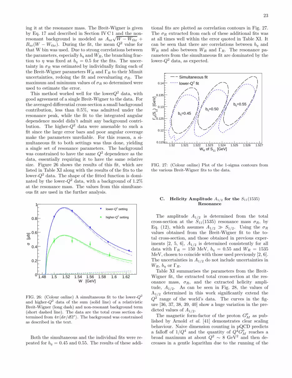
23

ing it at the resonance mass. The Breit-Wigner is givenby Eq. 17 and described in Section IVC 1 and the non-resonant background is modeled as Anr

√W − Wthr +

Bnr(W − Wthr). During the fit, the mean Q2 value forthat W bin was used. Due to strong correlations betweenthe parameters, especially bη and WR, the branching frac-tion to η was fixed at bη = 0.5 for the fits. The uncer-tainty in σR was estimated by individually fixing each ofthe Breit-Wigner parameters WR and ΓR to their Minuituncertainties, redoing the fit and reevaluating σR. Themaximum and minimum values of σR so determined wereused to estimate the error.

This method worked well for the lowerQ2 data, withgood agreement of a single Breit-Wigner to the data. Forthe averaged differential cross-section a small backgroundcontribution, less than 0.5%, was admitted under theresonance peak, while the fit to the integrated angulardependence model didn’t admit any background contri-bution. The higher-Q2 data were amenable to such afit since the large error bars and poor angular coveragemake the parameters unreliable. For this reason, a si-multaneous fit to both settings was thus done, yieldinga single set of resonance parameters. The backgroundwas constrained to have the same Q2 dependence as thedata, essentially requiring it to have the same relativesize. Figure 26 shows the results of this fit, which arelisted in Table XI along with the results of the fits to thelower-Q2 data. The shape of the fitted function is domi-nated by the lower-Q2 data, with a background of 1.2%at the resonance mass. The values from this simultane-ous fit are used in the further analysis.

W [GeV]1.48 1.5 1.52 1.54 1.56 1.58 1.6 1.62

b]µ

[σ

0

0.2

0.4

0.6

0.8

1 setting2lower-Q

setting2higher-Q

FIG. 26: (Colour online) A simultaneous fit to the lower-Q2

and higher-Q2 data of the sum (solid line) of a relativisticBreit-Wigner (long dash) and non-resonant background term(short dashed line). The data are the total cross section de-termined from 4π〈dσ/dΩ∗〉. The background was constrainedas described in the text.

Both the simultaneous and the individual fits were re-peated for bη = 0.45 and 0.55. The results of these addi-

tional fits are plotted as correlation contours in Fig. 27.The σR extracted from each of these additional fits wasat all times well within the error quoted in Table XI. Itcan be seen that there are correlations between bη andWR and also between WR and ΓR. The resonance pa-rameters from the simultaneous fit are dominated by thelower-Q2 data, as expected.

[GeV]11 of SRW1.52 1.521 1.522 1.523 1.524 1.525 1.526 1.527

) [G

eV]

11(S

RΓ

0.115

0.12

0.125

0.13

0.135

0.14

Simultaneous fit

fit2lower-Q

=0.55ηb

=0.45ηb=0.50ηb

FIG. 27: (Colour online) Plot of the 1-sigma contours fromthe various Breit-Wigner fits to the data.

C. Helicity Amplitude A1/2 for the S11(1535)Resonance

The amplitude A1/2 is determined from the totalcross-section at the S11(1535) resonance mass σR, byEq. (12), which assumes A1/2 ≫ S1/2. Using the σR

values obtained from the Breit-Wigner fit to the to-tal cross-section, and those obtained in previous exper-iments [2, 5, 6], A1/2 is determined consistently for alldata with ΓR = 150 MeV, bη = 0.55 and WR = 1535MeV, chosen to coincide with those used previously [2, 6].The uncertainties in A1/2 do not include uncertainties inWR, bη or ΓR.

Table XI summarises the parameters from the Breit-Wigner fit, the extracted total cross-section at the res-onance mass, σR, and the extracted helicity ampli-tude, A1/2. As can be seen in Fig. 28, the values ofA1/2 determined in this work significantly extend the

Q2 range of the world’s data. The curves in the fig-ure [36, 37, 38, 39, 40] show a huge variation in the pre-dicted values of A1/2.

The magnetic form-factor of the proton GpM as pub-

lished by Arnold et al. [41] demonstrates clear scalingbehaviour. Naive dimension counting in pQCD predictsa falloff of 1/Q4 and the quantity of Q4Gp

M reaches abroad maximum at about Q2 ∼ 8 GeV2 and then de-creases in a gentle logarithm due to the running of the

24

Q2(WR) WR ΓR σR A1/2

[GeV2/c2] [GeV] [GeV] [µb] [×10−3 GeV5/2]∫

dσ/dΩ∗|model indiv. 5.79 1.523 ± 0.001 0.125 ± 0.003 0.976 ± 0.007 23.62 ± 0.094π〈dσ/dΩ∗〉 5.79 1.523 ± 0.001 0.128 ± 0.010 0.977 ± 0.024 23.63 ± 0.304π〈dσ/dΩ∗〉 simul. Fig. 26 5.79 1.522 ± 0.001 0.128 ± 0.009 0.943 ± 0.015 23.22 ± 0.184π〈dσ/dΩ∗〉 Fig. 26 7.04 0.553 ± 0.020 17.79 ± 0.33

TABLE XI: Parameters extracted from a relativistic Breit-Wigner fit to the data. The values for A1/2(Q2) are determined

from σR, assuming A1/2 ≫ S1/2, with parameters WR = 1.53 GeV, ΓR = 150 MeV and bη = 0.55.

]2/c2 [GeV2Q0 1 2 3 4 5 6 7

]-1

/2

[GeV

1/2

A

0

0.02

0.04

0.06

0.08

0.1

0.12 Brasse (DESY) 1984Armstrong (JLab Hall C) 1999Denizli (JLab Hall B) 2007This work (JLab Hall C) 2007Aiello, Giannini and SantopintoCapstick and Keister, non-relCapstick and Keister, relKonen and WeberLi and ClosePace, Salme and Simula

FIG. 28: (Colour online) Values for A1/2(Q2) determined

from σR for the present and other data [2, 5, 6] (consistentlywith WR = 1.53 GeV, ΓR = 150 MeV and bη = 0.55). Thecurves are from Refs. [36, 37, 38, 39, 40].

strong coupling constant αs. The same arguments pre-dict that the helicity amplitude for the S11(1535) de-creases with 1/Q3. Figure 29 is a plot of Q3A1/2, showing

that the quantity Q3A1/2 appears to begin flattening ata photon momentum transfer broadly within the rangeof this work, Q2 ∼ 5 − 7 GeV2, a possible signal of theonset of pQCD scaling. A pQCD calculation by Carl-son and Poor [4], of the magnitude of this quantity, isplotted and is a factor of ∼ 3 smaller than the data. Ithas also been pointed out that such scaling may have anon-perturbative explanation [42, 43].

In order to compare the behaviour of A1/2 with the

approach of GpM to scaling, the quantity Q3A1/2/Q4Gp

Mis plotted in Fig. 30. The form of Gp

M is taken from the fitby Bosted [30]. The figure shows that the two quantitiesdon’t have the same form at low Q2, and the data doesn’tgo high enough in Q2 to know whether the two quantitiesbegin behaving equivalently.

]2/c2 [GeV2Q0 1 2 3 4 5 6 7

]5/

2

[GeV

1/2

A3Q

0

0.05

0.1

0.15

0.2

0.25

0.3

0.35

0.4Brasse (DESY) 1984Armstrong (JLab Hall C) 1999Denizli (JLab Hall B) 2007This work (JLab Hall C) 2008

FIG. 29: (Colour online) The Q2 dependence of Q3A1/2 forη-production. Scaling in this quantity appears to begin at aphoton momentum transfer of Q2 ∼ 5 GeV2. The dashed linesare a high Q2, pQCD calculation from Carlson and Poor [4]using three different nucleon distribution amplitudes.

]2/c2 [GeV2Q0 1 2 3 4 5 6 7

p MG4

) / Q

11(S

1/2

A3Q

0

0.05

0.1

0.15

0.2

0.25

0.3

Brasse (DESY) 1984

Armstrong (JLab Hall C) 1999

Denizli (JLab Hall B) 2007

This work (JLab Hall C) 2008

FIG. 30: (Colour online) The Q2 dependence ofQ3A1/2(S11)/Q4Gp

M for η-production.

25

VI. CONCLUSIONS

We have presented the results of a precise, high statis-tics measurement of the differential cross-section for theep → e′pη exclusive process. This is done at the highestmomentum transfer to date, namely, Q2 = 5.8 and 7.0(GeV/c)2 at the S11 resonance mass, which is a signif-icant extension from the previous highest at Q2 = 3.6GeV2. Data were obtained from threshold to W = 1.8GeV, the S11(1535) dominating the channel as expected.In the region from threshold to the S11(1535) resonancemass, the differential cross-section is largely isotropic—consistent with previous measurements.

The interference phenomenon in the linear cosθ∗η term

at W of the S11(1535) resonance mass, seen in lower Q2

and photoproduction data is observed here with simi-lar strength. The present data doesn’t have sufficientangular coverage at W ∼ 1.7 GeV to comment mean-ingfully on the strong presence of a P wave resonancethere. The curvature in the cosθ∗η dependence of the dif-ferential cross-section is opposite to that of the data atlower-Q2. The helicity-conserving transition amplitudeA1/2, is extracted from the data assuming no longitu-

dinal component (A1/2 ≫ S1/2). The Q2 dependence of

Q3A1/2 seems to be flattening, consistent with the pQCD

prediction, although the range of Q2 is too small to verifythe exact dependence. Even if the data scale as predictedby pQCD, that is not conclusive evidence for the onsetof pQCD.

On the theoretical front, the differential cross-sectionwill be incorporated into multi-channel, multi-resonancemodels, such as those by the maid and ebac groups,which should maximize the physics impact coming fromthese data. Also, the inability for any one calculationto adequately describe the Q2 dependence of A1/2 leavesmuch to be done in understanding the structure of theS11(1535). On the experimental front, more data arerequired to further address the questions in this paper.

It would be nice to fill the data gap in the region be-tween Q2 ∼ 4 and 5.8 GeV2 to analyse the apparentchange of differential cross-section shape. Extending thedata to Q2 much higher than 7 GeV2 will complete thestudy of the transition to hard-scale scattering. Obtain-ing LT separated data at high Q2 will enable checkingof the assumption, made in this work and in the litera-ture, that the longitudinal component is negligible. Theplanned upgrade of the Jefferson Lab accelerator, to en-ergies as high as 11 GeV, will allow exclusive η electro-production data to be obtained to Q2 ∼ 14 GeV2, andLT separations at least to the Q2 of this experiment.

Acknowledgments

We would like to acknowledge the support of staff andmanagement at Jefferson Lab.

This work is supported in part by research grants from

the U.S. Department of Energy (including grant DE-AC02-06CH11357), the U.S. National Science Founda-tion and the South African National Research Founda-tion.

The Southeastern Universities Research Associationoperates the Thomas Jefferson National Accelerator Fa-cility under the U.S. Department of Energy contractDEAC05-84ER40150.

APPENDIX: TABLES OF DIFFERENTIAL

CROSS-SECTIONS

TABLE XII: Lower-Q2 extracted differential cross-section.

W cosθ∗η φη 〈Q2

bin〉 〈ǫ〉 rad.corr.

d2σdΩ∗

ηδstat δsyst

[GeV] [deg.] [GeV2

c2] [nb

sr] [nb

sr] [nb

sr]

1.500 -0.917 22.5 5.80 0.427 1.51 60.6 8.3 3.61.500 -0.917 67.5 5.80 0.427 1.52 72.8 9.2 6.91.500 -0.917 112.5 5.80 0.426 1.49 59.1 8.0 4.61.500 -0.917 157.5 5.80 0.427 1.52 72.3 8.9 5.21.500 -0.917 202.5 5.80 0.426 1.50 65.1 8.5 5.51.500 -0.917 247.5 5.80 0.427 1.52 72.3 8.8 6.01.500 -0.917 292.5 5.80 0.426 1.52 67.0 8.4 6.21.500 -0.917 337.5 5.80 0.426 1.49 77.8 9.4 7.01.500 -0.750 22.5 5.80 0.427 1.53 85.5 9.8 5.21.500 -0.750 67.5 5.80 0.427 1.53 69.9 8.6 6.51.500 -0.750 112.5 5.81 0.426 1.48 59.2 7.9 4.71.500 -0.750 157.5 5.81 0.425 1.53 61.5 8.3 6.11.500 -0.750 202.5 5.79 0.427 1.52 62.3 8.0 4.51.500 -0.750 247.5 5.79 0.428 1.49 67.3 8.1 4.61.500 -0.750 292.5 5.80 0.427 1.51 70.8 8.4 3.71.500 -0.750 337.5 5.80 0.427 1.55 64.3 8.3 5.01.500 -0.583 22.5 5.80 0.427 1.54 57.7 8.4 4.01.500 -0.583 67.5 5.79 0.428 1.46 61.9 8.4 5.21.500 -0.583 112.5 5.80 0.427 1.53 60.1 8.2 6.31.500 -0.583 157.5 5.79 0.428 1.51 76.2 9.3 6.41.500 -0.583 202.5 5.78 0.428 1.46 71.0 8.6 3.81.500 -0.583 247.5 5.80 0.427 1.52 52.4 7.2 6.01.500 -0.583 292.5 5.79 0.428 1.51 66.9 8.7 7.21.500 -0.583 337.5 5.80 0.428 1.60 71.4 9.0 3.91.500 -0.417 22.5 5.81 0.426 1.53 52.3 8.6 3.11.500 -0.417 67.5 5.80 0.426 1.51 63.6 8.7 4.51.500 -0.417 112.5 5.80 0.427 1.53 54.9 7.9 5.21.500 -0.417 157.5 5.80 0.427 1.49 61.3 8.2 6.11.500 -0.417 202.5 5.79 0.428 1.48 58.3 8.1 3.21.500 -0.417 247.5 5.80 0.427 1.46 59.1 7.7 3.41.500 -0.417 292.5 5.80 0.427 1.51 62.2 7.8 6.81.500 -0.417 337.5 5.80 0.426 1.53 57.4 8.4 3.41.500 -0.250 22.5 5.81 0.426 1.52 78.5 9.9 6.91.500 -0.250 67.5 5.80 0.427 1.51 71.6 9.4 4.61.500 -0.250 112.5 5.80 0.427 1.48 83.6 9.6 7.31.500 -0.250 157.5 5.80 0.427 1.46 77.7 9.7 5.51.500 -0.250 202.5 5.79 0.428 1.47 76.3 9.2 6.61.500 -0.250 247.5 5.79 0.428 1.46 49.4 7.0 4.11.500 -0.250 292.5 5.80 0.428 1.53 42.5 6.7 4.41.500 -0.250 337.5 5.80 0.427 1.54 68.7 9.7 6.21.500 -0.083 22.5 5.82 0.424 1.56 67.9 10.1 3.71.500 -0.083 67.5 5.81 0.425 1.52 59.4 8.5 4.51.500 -0.083 112.5 5.81 0.424 1.46 59.1 8.1 4.51.500 -0.083 157.5 5.81 0.425 1.50 71.5 9.6 4.2

26

W cosθ∗η φη 〈Q2

bin〉 〈ǫ〉 rad.corr.

d2σdΩ∗

ηδstat δsyst

[GeV] [deg.] [GeV2

c2] [nb

sr] [nb

sr] [nb

sr]

1.500 -0.083 202.5 5.81 0.425 1.47 76.9 9.7 7.71.500 -0.083 247.5 5.80 0.426 1.49 59.1 7.4 4.71.500 -0.083 292.5 5.81 0.426 1.49 64.9 8.3 4.91.500 -0.083 337.5 5.81 0.426 1.51 64.3 9.6 5.81.500 0.083 22.5 5.82 0.424 1.53 82.9 10.8 7.51.500 0.083 67.5 5.81 0.426 1.49 60.9 8.7 3.91.500 0.083 112.5 5.81 0.426 1.50 74.4 9.3 4.71.500 0.083 157.5 5.80 0.426 1.47 81.2 10.5 5.21.500 0.083 202.5 5.80 0.427 1.47 64.9 9.3 5.31.500 0.083 247.5 5.81 0.426 1.49 65.1 8.1 6.31.500 0.083 292.5 5.81 0.425 1.49 58.6 8.4 3.51.500 0.083 337.5 5.82 0.424 1.51 54.2 9.2 3.31.500 0.250 22.5 5.81 0.427 1.51 68.9 10.4 6.61.500 0.250 67.5 5.80 0.428 1.48 57.7 9.0 3.81.500 0.250 112.5 5.80 0.427 1.43 70.0 9.5 4.61.500 0.250 157.5 5.79 0.429 1.46 77.5 10.3 6.51.500 0.250 202.5 5.80 0.427 1.47 70.5 9.7 3.41.500 0.250 247.5 5.80 0.427 1.48 49.6 7.9 4.51.500 0.250 292.5 5.80 0.427 1.49 61.3 9.3 4.61.500 0.250 337.5 5.81 0.426 1.51 62.4 10.2 6.31.500 0.417 22.5 5.81 0.427 1.52 60.4 10.1 4.21.500 0.417 67.5 5.80 0.428 1.50 73.5 10.1 5.91.500 0.417 112.5 5.80 0.427 1.47 71.5 8.9 5.61.500 0.417 157.5 5.80 0.427 1.45 61.7 9.9 5.41.500 0.417 202.5 5.81 0.426 1.43 66.3 9.7 3.61.500 0.417 247.5 5.81 0.427 1.49 63.3 8.5 4.91.500 0.417 292.5 5.80 0.428 1.48 45.4 8.4 2.91.500 0.417 337.5 5.81 0.426 1.51 66.4 10.6 4.41.500 0.583 22.5 5.81 0.427 1.50 61.9 10.2 5.61.500 0.583 67.5 5.81 0.427 1.47 73.6 9.8 4.41.500 0.583 112.5 5.81 0.426 1.45 66.9 9.0 5.11.500 0.583 157.5 5.80 0.427 1.45 66.1 9.7 4.31.500 0.583 202.5 5.80 0.427 1.46 80.5 10.5 5.21.500 0.583 247.5 5.81 0.426 1.47 79.9 9.7 4.01.500 0.583 292.5 5.80 0.428 1.47 66.9 9.7 4.11.500 0.583 337.5 5.81 0.426 1.48 71.5 10.8 5.01.500 0.750 22.5 5.81 0.427 1.43 63.0 10.6 4.61.500 0.750 67.5 5.80 0.428 1.47 50.8 8.8 3.71.500 0.750 112.5 5.80 0.427 1.42 70.3 9.4 5.81.500 0.750 157.5 5.81 0.426 1.43 68.3 9.9 5.21.500 0.750 202.5 5.81 0.426 1.42 70.6 10.3 5.21.500 0.750 247.5 5.81 0.425 1.46 66.5 9.5 4.51.500 0.750 292.5 5.80 0.427 1.45 87.3 10.6 5.61.500 0.750 337.5 5.80 0.427 1.48 75.8 11.4 4.01.500 0.917 22.5 5.79 0.429 1.47 77.5 11.2 4.41.500 0.917 67.5 5.81 0.427 1.44 79.6 10.8 5.71.500 0.917 112.5 5.81 0.426 1.45 70.1 10.5 4.51.500 0.917 157.5 5.81 0.426 1.40 80.2 10.7 6.41.500 0.917 202.5 5.81 0.427 1.44 73.0 10.6 4.11.500 0.917 247.5 5.81 0.426 1.42 70.4 10.2 5.41.500 0.917 292.5 5.80 0.427 1.45 60.6 10.2 4.21.500 0.917 337.5 5.80 0.427 1.47 65.8 11.3 4.51.530 -0.917 22.5 5.75 0.426 1.44 74.6 7.8 5.41.530 -0.917 67.5 5.76 0.425 1.40 62.4 6.9 7.51.530 -0.917 112.5 5.76 0.424 1.38 64.0 7.2 4.71.530 -0.917 157.5 5.76 0.424 1.41 57.9 6.6 6.51.530 -0.917 202.5 5.76 0.424 1.37 62.1 6.9 5.31.530 -0.917 247.5 5.76 0.424 1.40 70.1 7.1 4.21.530 -0.917 292.5 5.76 0.424 1.42 74.3 7.6 5.01.530 -0.917 337.5 5.75 0.425 1.42 70.1 7.5 4.11.530 -0.750 22.5 5.77 0.423 1.42 72.1 7.4 5.3

W cosθ∗η φη 〈Q2

bin〉 〈ǫ〉 rad.corr.

d2σdΩ∗

ηδstat δsyst

[GeV] [deg.] [GeV2

c2] [nb

sr] [nb

sr] [nb

sr]

1.530 -0.750 67.5 5.76 0.425 1.42 62.8 7.0 4.11.530 -0.750 112.5 5.75 0.424 1.38 78.2 7.6 4.61.530 -0.750 157.5 5.75 0.425 1.36 68.8 7.0 5.91.530 -0.750 202.5 5.75 0.425 1.34 71.7 7.1 4.41.530 -0.750 247.5 5.76 0.424 1.38 51.4 6.0 3.91.530 -0.750 292.5 5.76 0.424 1.37 67.9 7.0 3.91.530 -0.750 337.5 5.77 0.423 1.41 64.3 6.9 4.81.530 -0.583 22.5 5.77 0.422 1.41 74.2 8.1 4.31.530 -0.583 67.5 5.76 0.424 1.40 63.9 7.7 4.01.530 -0.583 112.5 5.76 0.424 1.38 68.0 7.8 5.51.530 -0.583 157.5 5.75 0.425 1.36 74.9 7.5 5.01.530 -0.583 202.5 5.75 0.425 1.36 60.9 6.7 4.41.530 -0.583 247.5 5.75 0.425 1.34 69.1 7.1 5.91.530 -0.583 292.5 5.77 0.423 1.38 69.1 7.5 4.31.530 -0.583 337.5 5.77 0.422 1.42 61.9 7.3 4.31.530 -0.417 22.5 5.76 0.424 1.40 79.8 8.6 5.41.530 -0.417 67.5 5.76 0.423 1.37 60.0 7.7 2.91.530 -0.417 112.5 5.76 0.424 1.34 63.7 7.5 6.01.530 -0.417 157.5 5.76 0.424 1.36 84.9 8.4 5.71.530 -0.417 202.5 5.76 0.424 1.32 77.4 7.7 4.11.530 -0.417 247.5 5.75 0.425 1.33 75.3 7.6 4.71.530 -0.417 292.5 5.77 0.423 1.33 81.2 8.3 4.41.530 -0.417 337.5 5.76 0.423 1.41 70.9 8.0 5.01.530 -0.250 22.5 5.75 0.425 1.43 88.8 9.9 5.21.530 -0.250 67.5 5.77 0.422 1.38 56.2 7.7 4.61.530 -0.250 112.5 5.77 0.422 1.32 68.2 8.3 4.21.530 -0.250 157.5 5.76 0.423 1.32 69.0 8.2 4.11.530 -0.250 202.5 5.76 0.423 1.35 77.5 8.2 4.91.530 -0.250 247.5 5.76 0.424 1.30 70.0 7.8 4.81.530 -0.250 292.5 5.77 0.422 1.34 69.2 8.0 3.61.530 -0.250 337.5 5.75 0.425 1.44 77.0 9.1 4.61.530 -0.083 22.5 5.76 0.424 1.42 69.7 9.9 4.21.530 -0.083 67.5 5.78 0.421 1.33 70.4 8.9 4.31.530 -0.083 112.5 5.78 0.421 1.30 58.1 7.7 3.31.530 -0.083 157.5 5.76 0.423 1.33 93.8 10.0 4.51.530 -0.083 202.5 5.76 0.423 1.33 72.1 8.6 3.71.530 -0.083 247.5 5.76 0.424 1.31 58.3 7.7 3.81.530 -0.083 292.5 5.77 0.423 1.32 62.1 8.1 3.21.530 -0.083 337.5 5.76 0.424 1.42 86.4 10.6 6.01.530 0.083 22.5 5.76 0.426 1.38 70.9 10.6 3.71.530 0.083 67.5 5.77 0.424 1.34 48.5 8.5 2.41.530 0.083 112.5 5.76 0.425 1.28 68.4 8.9 4.01.530 0.083 157.5 5.76 0.423 1.33 66.5 9.4 4.01.530 0.083 202.5 5.77 0.422 1.30 68.4 8.8 5.11.530 0.083 247.5 5.77 0.423 1.26 60.9 8.2 3.71.530 0.083 292.5 5.77 0.423 1.33 67.5 9.5 3.61.530 0.083 337.5 5.77 0.424 1.39 70.4 10.1 4.21.530 0.250 22.5 5.76 0.425 1.38 93.6 10.9 5.11.530 0.250 67.5 5.77 0.423 1.30 68.2 9.8 4.11.530 0.250 112.5 5.77 0.423 1.29 77.7 9.6 4.01.530 0.250 157.5 5.76 0.423 1.30 73.4 9.8 3.61.530 0.250 202.5 5.76 0.424 1.29 76.9 9.7 3.91.530 0.250 247.5 5.77 0.423 1.27 70.3 9.1 3.31.530 0.250 292.5 5.77 0.423 1.31 67.2 9.7 3.41.530 0.250 337.5 5.76 0.425 1.40 81.6 10.4 3.91.530 0.417 22.5 5.76 0.425 1.37 72.1 9.4 4.51.530 0.417 67.5 5.77 0.423 1.30 59.6 8.7 3.51.530 0.417 112.5 5.77 0.423 1.27 68.0 8.6 3.21.530 0.417 157.5 5.77 0.423 1.30 95.3 9.9 6.31.530 0.417 202.5 5.77 0.423 1.30 91.2 9.6 5.81.530 0.417 247.5 5.77 0.422 1.29 75.0 8.5 4.4

27

W cosθ∗η φη 〈Q2

bin〉 〈ǫ〉 rad.corr.

d2σdΩ∗

ηδstat δsyst

[GeV] [deg.] [GeV2

c2] [nb

sr] [nb

sr] [nb

sr]

1.530 0.417 292.5 5.77 0.423 1.32 84.1 9.7 5.01.530 0.417 337.5 5.77 0.424 1.38 94.7 10.3 4.81.530 0.583 22.5 5.77 0.423 1.36 77.4 11.2 5.61.530 0.583 67.5 5.77 0.423 1.27 81.7 10.4 4.71.530 0.583 112.5 5.77 0.422 1.28 63.0 8.8 4.71.530 0.583 157.5 5.77 0.422 1.30 84.8 10.5 4.61.530 0.583 202.5 5.77 0.423 1.30 95.2 11.1 4.61.530 0.583 247.5 5.77 0.423 1.29 94.1 10.2 5.41.530 0.583 292.5 5.76 0.424 1.32 84.2 10.8 6.01.530 0.583 337.5 5.77 0.423 1.40 72.9 10.5 3.71.530 0.750 22.5 5.79 0.421 1.33 87.7 12.3 4.71.530 0.750 67.5 5.77 0.423 1.31 73.2 11.0 4.41.530 0.750 112.5 5.77 0.423 1.28 75.5 10.6 3.71.530 0.750 157.5 5.77 0.422 1.29 93.1 11.7 7.21.530 0.750 202.5 5.77 0.423 1.32 77.5 10.8 4.31.530 0.750 247.5 5.77 0.423 1.32 82.0 10.1 4.61.530 0.750 292.5 5.77 0.423 1.32 68.4 10.8 5.01.530 0.750 337.5 5.79 0.421 1.35 78.4 11.3 6.31.530 0.917 22.5 5.78 0.423 1.31 94.7 12.6 7.51.530 0.917 67.5 5.76 0.425 1.31 86.5 11.8 5.71.530 0.917 112.5 5.77 0.424 1.31 104.3 11.6 6.21.530 0.917 157.5 5.77 0.423 1.30 77.4 10.5 5.21.530 0.917 202.5 5.77 0.423 1.31 106.5 11.6 5.91.530 0.917 247.5 5.77 0.423 1.31 102.1 11.5 5.11.530 0.917 292.5 5.77 0.424 1.31 77.8 11.2 4.61.530 0.917 337.5 5.77 0.423 1.31 106.0 12.8 7.41.560 -0.917 22.5 5.70 0.421 1.38 67.3 7.1 4.71.560 -0.917 67.5 5.70 0.421 1.36 62.2 7.0 3.71.560 -0.917 112.5 5.70 0.420 1.35 62.5 7.0 4.41.560 -0.917 157.5 5.69 0.422 1.33 67.8 7.0 4.41.560 -0.917 202.5 5.69 0.422 1.32 55.5 6.2 3.21.560 -0.917 247.5 5.70 0.421 1.34 59.5 6.2 4.31.560 -0.917 292.5 5.69 0.422 1.36 54.1 6.1 3.51.560 -0.917 337.5 5.70 0.420 1.38 55.7 6.6 3.21.560 -0.750 22.5 5.70 0.422 1.34 60.3 6.6 2.91.560 -0.750 67.5 5.69 0.422 1.32 53.6 6.3 3.81.560 -0.750 112.5 5.69 0.423 1.28 50.0 5.9 4.61.560 -0.750 157.5 5.68 0.423 1.25 54.2 6.1 3.81.560 -0.750 202.5 5.69 0.422 1.24 50.9 5.6 3.11.560 -0.750 247.5 5.69 0.422 1.31 54.6 5.9 2.81.560 -0.750 292.5 5.70 0.420 1.32 50.1 5.8 3.11.560 -0.750 337.5 5.70 0.421 1.35 52.9 6.1 2.81.560 -0.583 22.5 5.69 0.423 1.39 49.3 6.5 2.61.560 -0.583 67.5 5.71 0.420 1.34 46.8 6.9 2.91.560 -0.583 112.5 5.70 0.422 1.24 44.9 6.6 3.91.560 -0.583 157.5 5.70 0.421 1.27 49.4 6.1 3.41.560 -0.583 202.5 5.69 0.421 1.24 54.0 6.0 2.81.560 -0.583 247.5 5.70 0.421 1.26 42.0 5.8 2.51.560 -0.583 292.5 5.71 0.419 1.30 55.6 6.8 2.81.560 -0.583 337.5 5.69 0.422 1.36 52.5 6.4 2.81.560 -0.417 22.5 5.68 0.425 1.33 45.1 7.4 2.81.560 -0.417 67.5 5.72 0.419 1.26 49.9 7.7 2.91.560 -0.417 112.5 5.70 0.421 1.23 43.7 7.0 2.71.560 -0.417 157.5 5.69 0.421 1.26 53.6 6.9 3.01.560 -0.417 202.5 5.70 0.420 1.24 57.5 6.8 3.71.560 -0.417 247.5 5.69 0.422 1.17 38.6 6.3 3.01.560 -0.417 292.5 5.72 0.419 1.24 46.3 6.9 3.11.560 -0.417 337.5 5.68 0.425 1.30 52.6 7.5 2.91.560 -0.250 22.5 5.68 0.424 1.28 54.9 9.1 2.91.560 -0.250 67.5 5.71 0.419 1.20 42.9 7.5 3.11.560 -0.250 112.5 5.70 0.420 1.16 40.5 7.2 2.1

W cosθ∗η φη 〈Q2

bin〉 〈ǫ〉 rad.corr.

d2σdΩ∗

ηδstat δsyst

[GeV] [deg.] [GeV2

c2] [nb

sr] [nb

sr] [nb

sr]

1.560 -0.250 157.5 5.69 0.421 1.22 56.5 7.6 2.71.560 -0.250 202.5 5.70 0.420 1.23 59.6 7.1 4.31.560 -0.250 247.5 5.71 0.419 1.16 51.1 7.2 2.91.560 -0.250 292.5 5.72 0.419 1.20 40.8 6.9 4.51.560 -0.250 337.5 5.68 0.425 1.30 41.6 8.1 3.11.560 -0.083 22.5 5.70 0.422 1.27 54.3 10.3 3.61.560 -0.083 67.5 5.73 0.417 1.15 32.9 8.1 2.21.560 -0.083 112.5 5.72 0.419 1.06 38.8 7.5 4.11.560 -0.083 157.5 5.71 0.419 1.21 64.5 8.7 4.11.560 -0.083 202.5 5.70 0.420 1.19 57.9 7.9 3.31.560 -0.083 247.5 5.72 0.420 1.07 70.5 9.5 3.91.560 -0.083 292.5 5.72 0.420 1.17 51.9 8.8 3.41.560 -0.083 337.5 5.69 0.423 1.26 41.8 8.8 2.91.560 0.083 22.5 5.68 0.426 1.24 61.5 10.1 3.21.560 0.083 67.5 5.72 0.420 1.10 48.4 10.5 2.81.560 0.083 112.5 5.72 0.419 1.00 50.7 10.3 5.61.560 0.083 157.5 5.69 0.421 1.19 56.0 9.2 3.31.560 0.083 202.5 5.70 0.420 1.19 60.6 8.7 3.31.560 0.083 247.5 5.74 0.418 1.02 44.3 8.9 3.31.560 0.083 292.5 5.73 0.419 1.11 54.5 10.2 3.21.560 0.083 337.5 5.69 0.424 1.27 56.8 9.7 3.41.560 0.250 22.5 5.69 0.424 1.23 44.5 9.0 2.51.560 0.250 67.5 5.73 0.419 1.06 30.8 9.7 2.01.560 0.250 112.5 5.74 0.417 0.98 47.0 9.9 2.71.560 0.250 157.5 5.70 0.420 1.14 43.3 8.8 2.61.560 0.250 202.5 5.70 0.421 1.16 48.1 8.4 3.21.560 0.250 247.5 5.74 0.417 0.99 51.9 9.4 2.71.560 0.250 292.5 5.74 0.418 1.07 55.8 10.8 2.81.560 0.250 337.5 5.69 0.424 1.25 47.9 9.1 2.21.560 0.417 22.5 5.69 0.424 1.20 49.5 9.5 2.61.560 0.417 67.5 5.73 0.418 1.05 49.8 10.7 3.11.560 0.417 112.5 5.73 0.418 1.00 48.4 9.4 4.81.560 0.417 157.5 5.70 0.420 1.13 51.8 9.3 3.11.560 0.417 202.5 5.70 0.420 1.13 50.0 8.8 4.81.560 0.417 247.5 5.73 0.418 1.01 53.0 9.4 4.11.560 0.417 292.5 5.73 0.418 1.10 55.3 10.3 3.61.560 0.417 337.5 5.69 0.424 1.25 64.1 9.7 3.71.560 0.583 22.5 5.71 0.420 1.17 65.6 11.9 4.31.560 0.583 67.5 5.74 0.416 1.05 61.8 11.8 4.01.560 0.583 112.5 5.72 0.418 1.03 53.2 10.8 2.91.560 0.583 157.5 5.71 0.419 1.11 56.0 11.3 4.51.560 0.583 202.5 5.71 0.419 1.13 53.0 10.3 2.51.560 0.583 247.5 5.72 0.418 1.05 44.3 10.1 3.81.560 0.583 292.5 5.74 0.417 1.08 54.8 11.3 3.41.560 0.583 337.5 5.71 0.421 1.21 63.4 11.0 3.31.560 0.750 22.5 5.71 0.421 1.12 75.8 14.4 5.61.560 0.750 67.5 5.70 0.422 1.09 67.5 13.0 4.21.560 0.750 112.5 5.70 0.421 1.08 62.0 11.2 4.21.560 0.750 157.5 5.71 0.420 1.14 60.4 10.6 2.81.560 0.750 202.5 5.71 0.420 1.15 67.9 10.3 3.51.560 0.750 247.5 5.72 0.419 1.12 67.2 10.1 5.51.560 0.750 292.5 5.71 0.420 1.13 65.2 11.6 4.21.560 0.750 337.5 5.73 0.419 1.12 86.2 13.5 4.01.560 0.917 22.5 5.69 0.424 1.19 88.8 14.5 4.31.560 0.917 67.5 5.69 0.424 1.17 87.7 13.1 4.91.560 0.917 112.5 5.70 0.422 1.17 65.3 11.6 4.41.560 0.917 157.5 5.70 0.422 1.18 72.7 11.8 3.61.560 0.917 202.5 5.70 0.421 1.17 67.3 11.2 3.81.560 0.917 247.5 5.70 0.422 1.19 64.9 11.1 4.41.560 0.917 292.5 5.69 0.424 1.18 81.9 12.9 4.51.560 0.917 337.5 5.69 0.425 1.21 77.9 14.3 4.5

28

W cosθ∗η φη 〈Q2

bin〉 〈ǫ〉 rad.corr.

d2σdΩ∗

ηδstat δsyst

[GeV] [deg.] [GeV2

c2] [nb

sr] [nb

sr] [nb

sr]

1.590 -0.917 22.5 5.64 0.417 1.41 61.2 6.6 3.91.590 -0.917 67.5 5.63 0.418 1.37 46.9 6.2 2.61.590 -0.917 112.5 5.63 0.418 1.32 63.8 7.2 5.01.590 -0.917 157.5 5.63 0.419 1.33 37.4 5.8 2.91.590 -0.917 202.5 5.63 0.419 1.32 45.1 5.8 3.01.590 -0.917 247.5 5.63 0.418 1.29 41.3 5.5 2.31.590 -0.917 292.5 5.63 0.420 1.34 42.4 5.6 2.71.590 -0.917 337.5 5.64 0.417 1.38 42.5 5.5 2.61.590 -0.750 22.5 5.62 0.421 1.31 49.0 6.2 2.81.590 -0.750 67.5 5.64 0.418 1.29 47.8 6.3 3.21.590 -0.750 112.5 5.63 0.418 1.24 49.0 6.3 2.91.590 -0.750 157.5 5.63 0.419 1.21 47.4 5.8 2.61.590 -0.750 202.5 5.63 0.419 1.22 40.4 5.1 3.11.590 -0.750 247.5 5.63 0.419 1.22 29.3 4.8 2.11.590 -0.750 292.5 5.64 0.417 1.28 30.0 4.8 1.51.590 -0.750 337.5 5.62 0.420 1.32 37.9 5.2 2.31.590 -0.583 22.5 5.61 0.422 1.31 45.4 6.8 2.41.590 -0.583 67.5 5.64 0.418 1.28 34.8 6.1 2.91.590 -0.583 112.5 5.64 0.417 1.25 32.8 5.9 3.51.590 -0.583 157.5 5.63 0.418 1.22 38.8 5.5 2.81.590 -0.583 202.5 5.63 0.418 1.22 33.6 5.1 2.81.590 -0.583 247.5 5.63 0.419 1.19 43.3 6.6 3.31.590 -0.583 292.5 5.64 0.418 1.24 39.1 6.2 2.61.590 -0.583 337.5 5.62 0.421 1.34 39.1 6.3 2.31.590 -0.417 22.5 5.62 0.421 1.27 35.5 8.0 3.71.590 -0.417 67.5 5.65 0.417 1.15 16.3 5.9 1.81.590 -0.417 112.5 5.64 0.418 1.09 23.0 6.0 2.71.590 -0.417 157.5 5.63 0.417 1.19 43.1 6.4 3.91.590 -0.417 202.5 5.63 0.419 1.19 37.9 6.0 2.81.590 -0.417 247.5 5.65 0.416 1.08 36.5 7.2 2.31.590 -0.417 292.5 5.65 0.417 1.16 30.9 6.9 1.91.590 -0.417 337.5 5.62 0.421 1.29 33.5 7.5 2.41.590 -0.250 22.5 5.61 0.423 1.26 32.9 9.6 2.41.590 -0.250 67.5 5.66 0.416 1.08 21.6 7.8 2.11.590 -0.250 112.5 5.65 0.416 1.06 22.7 7.1 2.91.590 -0.250 157.5 5.63 0.418 1.18 35.6 7.0 2.11.590 -0.250 202.5 5.62 0.419 1.15 33.2 6.6 2.11.590 -0.250 247.5 5.66 0.415 1.01 31.9 7.8 4.01.590 -0.250 292.5 5.65 0.417 1.11 38.7 8.7 4.11.590 -0.250 337.5 5.61 0.424 1.27 35.7 9.0 2.41.590 -0.083 22.5 5.59 0.427 1.18 21.0 9.2 3.21.590 -0.083 67.5 5.65 0.417 0.95 19.3 9.2 1.21.590 -0.083 112.5 5.68 0.414 0.86 22.3 8.9 2.01.590 -0.083 157.5 5.64 0.416 1.13 32.4 7.7 1.91.590 -0.083 202.5 5.63 0.418 1.12 40.1 7.2 2.91.590 -0.083 247.5 5.67 0.416 0.89 32.8 9.7 4.31.590 -0.083 292.5 5.67 0.415 0.98 27.1 9.3 5.01.590 -0.083 337.5 5.59 0.427 1.21 33.4 9.9 3.11.590 0.083 22.5 5.58 0.431 1.15 29.2 9.9 1.91.590 0.083 112.5 5.64 0.419 0.75 26.2 11.5 6.01.590 0.083 157.5 5.63 0.419 1.12 33.7 8.3 2.31.590 0.083 202.5 5.63 0.417 1.11 35.6 8.1 1.91.590 0.083 247.5 5.68 0.415 0.79 35.4 13.2 4.71.590 0.083 292.5 5.67 0.417 0.88 48.8 14.3 5.71.590 0.083 337.5 5.57 0.431 1.16 55.6 11.9 5.31.590 0.250 22.5 5.58 0.431 1.07 30.3 11.5 4.61.590 0.250 112.5 5.65 0.417 0.66 24.2 13.1 4.11.590 0.250 157.5 5.63 0.417 1.05 25.0 8.9 3.71.590 0.250 202.5 5.63 0.418 1.06 36.7 8.7 3.31.590 0.250 247.5 5.67 0.416 0.70 37.9 13.0 3.81.590 0.250 292.5 5.68 0.415 0.87 22.7 11.0 2.2

W cosθ∗η φη 〈Q2

bin〉 〈ǫ〉 rad.corr.

d2σdΩ∗

ηδstat δsyst

[GeV] [deg.] [GeV2

c2] [nb

sr] [nb

sr] [nb

sr]

1.590 0.250 337.5 5.59 0.429 1.08 41.8 11.4 3.91.590 0.417 22.5 5.59 0.429 1.09 45.2 13.0 3.11.590 0.417 67.5 5.68 0.414 0.77 39.0 14.3 4.01.590 0.417 112.5 5.67 0.415 0.68 39.2 13.8 5.51.590 0.417 157.5 5.65 0.416 1.05 27.4 9.9 2.41.590 0.417 202.5 5.65 0.416 1.07 40.7 9.8 2.51.590 0.417 247.5 5.64 0.419 0.75 25.8 12.8 2.41.590 0.417 292.5 5.67 0.417 0.86 52.8 14.9 5.91.590 0.417 337.5 5.58 0.431 1.06 48.7 12.7 3.71.590 0.583 22.5 5.65 0.419 0.92 51.5 17.1 4.51.590 0.583 67.5 5.71 0.411 0.71 38.5 16.7 4.71.590 0.583 112.5 5.67 0.415 0.67 34.2 14.7 4.91.590 0.583 157.5 5.64 0.417 1.00 38.1 11.8 3.51.590 0.583 202.5 5.64 0.417 1.02 31.6 10.3 2.11.590 0.583 247.5 5.66 0.415 0.76 47.7 14.8 4.01.590 0.583 292.5 5.71 0.410 0.81 52.4 17.0 4.11.590 0.583 337.5 5.65 0.420 0.95 31.3 13.1 5.41.590 0.750 22.5 5.60 0.426 0.92 58.3 22.2 13.01.590 0.750 67.5 5.63 0.420 0.85 29.3 15.9 4.11.590 0.750 112.5 5.65 0.417 0.89 30.4 11.5 4.01.590 0.750 157.5 5.64 0.417 1.05 29.7 11.1 2.81.590 0.750 202.5 5.64 0.417 1.05 35.4 10.1 2.61.590 0.750 247.5 5.65 0.416 0.94 39.1 11.9 3.11.590 0.750 292.5 5.63 0.421 0.92 61.9 16.8 3.51.590 0.750 337.5 5.61 0.426 0.91 67.8 20.9 7.21.590 0.917 67.5 5.66 0.415 1.03 25.0 14.4 4.01.590 0.917 112.5 5.66 0.415 1.03 23.5 12.8 2.41.590 0.917 247.5 5.65 0.417 1.05 24.6 12.1 1.61.590 0.917 337.5 5.64 0.421 1.05 39.8 18.0 3.01.625 -0.917 22.5 5.56 0.414 1.41 33.6 4.7 2.21.625 -0.917 67.5 5.56 0.415 1.36 33.2 4.8 3.31.625 -0.917 112.5 5.55 0.416 1.34 36.3 5.0 2.11.625 -0.917 157.5 5.55 0.415 1.32 24.5 4.4 1.81.625 -0.917 202.5 5.55 0.416 1.30 33.9 4.6 2.21.625 -0.917 247.5 5.55 0.415 1.32 23.4 4.0 1.71.625 -0.917 292.5 5.55 0.416 1.33 32.2 4.4 2.01.625 -0.917 337.5 5.56 0.415 1.40 28.2 4.3 2.81.625 -0.750 22.5 5.54 0.419 1.35 37.2 5.5 2.21.625 -0.750 67.5 5.56 0.414 1.30 27.7 4.8 1.71.625 -0.750 112.5 5.56 0.415 1.24 37.3 5.5 2.91.625 -0.750 157.5 5.55 0.415 1.23 35.4 4.9 2.51.625 -0.750 202.5 5.55 0.415 1.21 24.8 4.1 1.31.625 -0.750 247.5 5.55 0.416 1.21 36.4 4.9 2.61.625 -0.750 292.5 5.57 0.414 1.28 23.5 4.2 1.81.625 -0.750 337.5 5.54 0.419 1.33 30.4 4.8 1.71.625 -0.583 22.5 5.53 0.420 1.33 35.0 6.3 2.21.625 -0.583 67.5 5.57 0.415 1.24 25.6 5.9 3.61.625 -0.583 112.5 5.55 0.417 1.17 23.1 5.4 2.31.625 -0.583 157.5 5.54 0.417 1.20 34.6 4.9 2.31.625 -0.583 202.5 5.55 0.415 1.21 30.9 4.6 1.91.625 -0.583 247.5 5.56 0.415 1.13 18.2 4.7 2.21.625 -0.583 292.5 5.56 0.416 1.21 18.3 4.9 1.31.625 -0.583 337.5 5.54 0.419 1.30 29.5 6.1 2.51.625 -0.417 22.5 5.52 0.423 1.25 22.3 7.7 1.71.625 -0.417 157.5 5.55 0.415 1.14 28.7 5.6 1.71.625 -0.417 202.5 5.55 0.416 1.15 23.3 5.1 1.21.625 -0.417 247.5 5.57 0.415 0.93 23.8 6.7 3.11.625 -0.417 292.5 5.57 0.414 1.06 14.9 6.5 2.11.625 -0.417 337.5 5.52 0.423 1.29 22.7 7.6 1.61.625 -0.250 67.5 5.57 0.417 0.90 16.6 8.9 3.21.625 -0.250 157.5 5.56 0.414 1.15 25.5 6.6 1.4

29

W cosθ∗η φη 〈Q2

bin〉 〈ǫ〉 rad.corr.

d2σdΩ∗

ηδstat δsyst

[GeV] [deg.] [GeV2

c2] [nb

sr] [nb

sr] [nb

sr]

1.625 -0.250 202.5 5.56 0.414 1.10 23.1 5.8 1.21.625 -0.250 247.5 5.56 0.416 0.85 38.6 10.8 5.01.625 -0.250 292.5 5.56 0.417 0.96 21.7 9.3 2.51.625 -0.083 157.5 5.57 0.412 1.08 15.5 7.1 1.01.625 -0.083 202.5 5.57 0.413 1.07 14.4 6.5 1.51.625 0.083 157.5 5.56 0.415 1.05 13.5 8.3 1.11.625 0.083 202.5 5.56 0.414 1.07 18.8 7.6 1.41.625 0.250 157.5 5.56 0.414 1.02 15.9 8.9 2.41.625 0.250 202.5 5.56 0.414 1.00 19.2 8.7 1.61.625 0.417 202.5 5.57 0.412 0.98 23.7 9.9 2.01.625 0.583 202.5 5.57 0.413 0.96 20.3 10.7 1.31.625 0.750 112.5 5.62 0.409 0.63 23.3 13.3 1.71.665 -0.917 22.5 5.46 0.413 1.39 24.6 4.6 2.01.665 -0.917 67.5 5.46 0.412 1.38 20.6 4.7 1.51.665 -0.917 112.5 5.45 0.413 1.34 19.3 4.7 2.01.665 -0.917 157.5 5.45 0.413 1.32 26.1 4.6 1.71.665 -0.917 202.5 5.45 0.413 1.33 15.3 4.0 2.01.665 -0.917 247.5 5.45 0.413 1.33 23.9 4.6 1.91.665 -0.917 292.5 5.46 0.412 1.35 31.3 4.9 3.41.665 -0.917 337.5 5.46 0.413 1.37 21.6 4.3 2.01.665 -0.750 22.5 5.45 0.415 1.34 26.5 6.1 1.71.665 -0.750 67.5 5.46 0.412 1.31 14.8 4.7 1.71.665 -0.750 112.5 5.46 0.412 1.23 17.3 4.7 1.51.665 -0.750 157.5 5.46 0.412 1.23 21.8 4.6 1.71.665 -0.750 202.5 5.46 0.412 1.23 22.2 4.3 1.51.665 -0.750 247.5 5.45 0.412 1.20 24.8 4.9 1.91.665 -0.750 292.5 5.46 0.412 1.25 25.6 4.8 1.61.665 -0.750 337.5 5.44 0.416 1.33 22.7 5.5 2.51.665 -0.583 22.5 5.42 0.421 1.31 17.6 7.4 2.81.665 -0.583 67.5 5.48 0.412 1.18 16.2 7.2 3.01.665 -0.583 112.5 5.48 0.410 1.17 12.7 5.7 2.91.665 -0.583 157.5 5.45 0.413 1.21 16.6 5.0 2.01.665 -0.583 202.5 5.45 0.413 1.19 18.4 4.7 1.01.665 -0.583 247.5 5.49 0.408 1.11 14.0 5.9 1.71.665 -0.583 292.5 5.46 0.413 1.19 21.3 7.3 2.01.665 -0.583 337.5 5.42 0.420 1.29 17.2 7.4 1.61.665 -0.417 157.5 5.46 0.411 1.15 15.2 5.6 1.21.665 -0.417 202.5 5.46 0.411 1.16 13.1 5.2 1.11.665 -0.250 157.5 5.47 0.409 1.12 11.4 6.4 2.01.665 -0.250 202.5 5.47 0.410 1.10 10.4 5.9 2.01.705 -0.917 22.5 5.35 0.411 1.39 20.8 5.0 1.41.705 -0.917 67.5 5.36 0.409 1.35 18.4 5.1 1.61.705 -0.917 112.5 5.36 0.409 1.35 21.2 5.5 1.81.705 -0.917 157.5 5.35 0.410 1.33 22.0 4.8 1.51.705 -0.917 202.5 5.35 0.410 1.32 21.2 4.6 1.41.705 -0.917 247.5 5.35 0.410 1.31 26.5 5.3 2.01.705 -0.917 292.5 5.35 0.409 1.33 18.5 4.5 1.21.705 -0.917 337.5 5.35 0.411 1.38 24.6 4.8 1.81.705 -0.750 22.5 5.34 0.412 1.36 22.7 7.4 1.71.705 -0.750 67.5 5.36 0.409 1.27 12.1 5.2 1.61.705 -0.750 112.5 5.36 0.408 1.23 15.9 5.3 2.21.705 -0.750 157.5 5.35 0.409 1.24 20.6 5.0 1.41.705 -0.750 202.5 5.35 0.409 1.24 11.9 4.3 1.51.705 -0.750 247.5 5.35 0.409 1.19 17.2 5.3 2.81.705 -0.750 292.5 5.35 0.410 1.26 23.2 5.4 1.61.705 -0.750 337.5 5.34 0.412 1.35 21.8 6.5 3.11.705 -0.583 157.5 5.35 0.410 1.21 13.8 5.8 1.11.705 -0.583 202.5 5.35 0.410 1.19 11.9 5.4 1.81.745 -0.917 22.5 5.25 0.408 1.41 19.0 5.1 2.11.745 -0.917 67.5 5.25 0.407 1.36 16.6 5.3 2.11.745 -0.917 112.5 5.25 0.407 1.34 8.2 4.7 1.1

W cosθ∗η φη 〈Q2

bin〉 〈ǫ〉 rad.corr.

d2σdΩ∗

ηδstat δsyst

[GeV] [deg.] [GeV2

c2] [nb

sr] [nb

sr] [nb

sr]

1.745 -0.917 157.5 5.24 0.408 1.32 13.5 4.7 1.31.745 -0.917 202.5 5.24 0.407 1.32 13.3 4.6 1.51.745 -0.917 247.5 5.25 0.407 1.34 18.7 5.0 2.61.745 -0.917 292.5 5.25 0.407 1.37 15.5 4.7 1.21.745 -0.917 337.5 5.24 0.409 1.38 17.4 4.8 1.31.745 -0.750 22.5 5.22 0.412 1.42 20.9 8.6 4.11.745 -0.750 67.5 5.26 0.406 1.29 16.0 5.8 2.21.745 -0.750 112.5 5.26 0.407 1.28 12.7 5.5 1.01.745 -0.750 157.5 5.25 0.406 1.26 14.1 5.0 1.61.745 -0.750 202.5 5.25 0.407 1.24 9.0 4.4 0.71.745 -0.750 247.5 5.25 0.407 1.15 9.2 5.2 0.91.745 -0.750 292.5 5.25 0.408 1.22 13.7 5.7 2.41.745 -0.750 337.5 5.23 0.412 1.33 16.2 8.2 4.71.785 -0.917 22.5 5.13 0.407 1.37 19.2 5.6 4.41.785 -0.917 112.5 5.14 0.405 1.36 11.5 5.4 1.01.785 -0.917 247.5 5.14 0.406 1.31 8.8 4.8 0.71.785 -0.917 337.5 5.13 0.407 1.38 13.5 5.1 1.91.785 -0.750 157.5 5.14 0.404 1.26 14.3 5.4 1.31.830 -0.917 22.5 5.02 0.406 1.37 18.4 5.9 1.71.830 -0.917 67.5 5.03 0.404 1.37 12.5 5.0 1.41.830 -0.917 112.5 5.03 0.404 1.35 17.8 6.2 1.81.830 -0.917 247.5 5.02 0.405 1.29 13.4 5.6 1.31.830 -0.917 292.5 5.02 0.405 1.35 10.4 5.0 1.21.830 -0.917 337.5 5.02 0.405 1.38 9.0 5.1 2.41.830 -0.750 157.5 5.03 0.403 1.27 11.4 5.8 0.8

TABLE XIII: Higher-Q2 extracted differential cross-section.

W cosθ∗η φη 〈Q2

bin〉 〈ǫ〉 rad.corr.

d2σdΩ∗

ηδstat δsyst

[GeV] [deg.] [GeV2

c2] [nb

sr] [nb

sr] [nb

sr]

1.500 -0.833 36.0 7.04 0.216 1.52 49.4 14.2 3.41.500 -0.833 108.0 7.06 0.211 1.56 32.7 7.6 1.51.500 -0.833 180.0 7.07 0.210 1.57 36.9 7.8 2.01.500 -0.833 252.0 7.06 0.210 1.54 38.9 7.8 2.31.500 -0.833 324.0 7.04 0.216 1.53 36.4 12.3 2.01.500 -0.500 108.0 7.06 0.211 1.53 35.8 8.1 2.01.500 -0.500 180.0 7.07 0.210 1.53 36.5 7.8 1.81.500 -0.500 252.0 7.06 0.211 1.53 42.6 7.9 2.11.500 -0.167 108.0 7.07 0.210 1.52 33.8 9.0 1.91.500 -0.167 180.0 7.08 0.208 1.50 40.8 10.5 2.51.500 -0.167 252.0 7.07 0.209 1.52 50.0 10.0 3.31.500 0.167 180.0 7.07 0.209 1.45 38.0 15.3 2.71.500 0.167 252.0 7.06 0.212 1.48 38.5 13.6 2.21.530 -0.833 36.0 6.97 0.216 1.30 24.2 11.3 2.11.530 -0.833 108.0 7.01 0.209 1.40 38.5 6.6 2.31.530 -0.833 180.0 7.01 0.208 1.37 42.6 6.5 2.31.530 -0.833 252.0 7.01 0.209 1.38 55.2 7.4 2.71.530 -0.833 324.0 6.97 0.216 1.31 43.4 14.2 2.91.530 -0.500 108.0 7.00 0.210 1.38 43.1 7.8 1.91.530 -0.500 180.0 7.01 0.208 1.36 34.8 6.7 1.91.530 -0.500 252.0 7.01 0.210 1.37 31.6 6.3 1.51.530 -0.167 108.0 7.02 0.208 1.38 37.4 8.5 1.81.530 -0.167 180.0 7.05 0.204 1.33 47.1 10.5 2.31.530 -0.167 252.0 7.02 0.208 1.37 28.7 7.3 1.71.560 -0.833 108.0 6.93 0.208 1.27 34.5 6.0 1.61.560 -0.833 180.0 6.94 0.207 1.26 42.4 6.0 2.11.560 -0.833 252.0 6.93 0.208 1.26 37.9 5.8 1.9

30

W cosθ∗η φη 〈Q2

bin〉 〈ǫ〉 rad.corr.

d2σdΩ∗

ηδstat δsyst

[GeV] [deg.] [GeV2

c2] [nb

sr] [nb

sr] [nb

sr]

1.560 -0.500 108.0 6.94 0.207 1.25 35.6 6.5 1.71.560 -0.500 180.0 6.95 0.206 1.24 37.5 6.2 1.71.560 -0.500 252.0 6.94 0.208 1.22 40.9 6.6 1.91.560 -0.167 108.0 6.95 0.205 1.22 21.8 7.4 1.21.560 -0.167 180.0 6.96 0.204 1.25 33.0 10.9 2.11.560 -0.167 252.0 6.96 0.205 1.24 22.3 6.8 1.11.560 0.167 252.0 6.97 0.203 1.03 50.8 19.5 9.11.592 -0.833 108.0 6.85 0.207 1.18 19.3 4.5 1.31.592 -0.833 180.0 6.86 0.206 1.16 27.5 4.6 1.21.592 -0.833 252.0 6.85 0.207 1.17 20.5 4.3 0.91.592 -0.500 108.0 6.86 0.205 1.19 19.8 5.1 1.01.592 -0.500 180.0 6.87 0.204 1.19 24.1 5.1 1.21.592 -0.500 252.0 6.86 0.205 1.16 22.6 5.7 1.4

1.592 -0.167 108.0 6.89 0.202 1.05 29.5 10.1 1.51.635 -0.833 108.0 6.74 0.205 1.15 28.0 5.4 1.51.635 -0.833 180.0 6.75 0.203 1.15 21.8 4.3 1.11.635 -0.833 252.0 6.74 0.205 1.17 16.9 4.2 0.91.635 -0.500 108.0 6.76 0.203 1.13 16.5 5.3 0.91.635 -0.500 180.0 6.75 0.203 1.18 10.3 4.6 0.61.685 -0.833 108.0 6.60 0.203 1.26 11.8 5.6 0.71.685 -0.833 252.0 6.60 0.203 1.27 12.0 4.9 0.91.685 -0.500 180.0 6.60 0.202 1.19 15.8 4.9 0.71.740 -0.833 180.0 6.46 0.201 1.30 18.3 4.7 1.0

[1] W. M. Yao et al. (Particle Data Group), J. Phys. G33,1 (2006).

[2] C. S. Armstrong, P. Stoler, et al., Phys. Rev. D60,052004 (1999).

[3] F. W. Brasse et al., Nucl. Phys. B139, 37 (1978).[4] C. E. Carlson and J. L. Poor, Phys. Rev. D38, 2758

(1988).[5] F. W. Brasse et al., Z. Phys. C22, 33 (1984).[6] H. Denizli et al. (CLAS), Phys. Rev. C76, 015204 (2007),

arXiv:0704.2546 [nucl-ex].[7] L. N. Hand, Phys. Rev. 129, 1834 (1963).[8] R. L. Walker, Phys. Rev. 182, 1729 (1969).[9] M. Warns, H. Schroder, W. Pfeil, and H. Rollnik, Z.

Phys. C45, 627 (1990).[10] G. Knochlein, D. Drechsel, and L. Tiator, Z. Phys. A352,

327 (1995), nucl-th/9506029.[11] D. Drechsel and L. Tiator, J. Phys. G18, 449 (1992).[12] Particle Data Group, Rev. Mod. Phys. 48, S157 (1976).[13] B. Krusche et al., Phys. Rev. Lett. 74, 3736 (1995).[14] H. Breuker et al., Phys. Lett. B74, 409 (1978).[15] F. Ravndal, Phys. Rev. D4, 1466 (1971).[16] R. M. Mohring, Ph.D. thesis, University of Maryland

(1999), uMI-99-57190.[17] J. R. Arrington, Ph.D. thesis, California Institute of

Technology (1998), nucl-ex/0608013.[18] C. W. Leemann, D. R. Douglas, and G. A. Krafft, Ann.

Rev. Nucl. Part. Sci. 51, 413 (2001).[19] H. P. Blok et al. (Jefferson Lab), Phys. Rev. C78, 045202

(2008), 0809.3161.[20] A. Villano, Ph.D. thesis, Rensselaer Polytechnic Institute

(2007).[21] T. Horn, Ph.D. thesis, University of Maryland (2006).[22] J. Arrington, Hall C in house publication, A-B-SIMC

(2001).[23] K. Makino and M. Berz, Nucl. Instrum. Meth. A558,

346 (2006).[24] M. E. Christy and P. B. Bosted (2007), arXiv:0712.3731

[hep-ph].[25] P. Corvisiero et al., Nucl. Instrum. Meth. A346, 433

(1994).[26] V. I. Mokeev et al., Phys. Atom. Nucl. 64, 1292 (2001).[27] M. Ripani et al., Phys. Rev. Lett. 91, 022002 (2003).[28] F. James and M. Roos, Comput. Phys. Commun. 10, 343

(1975).[29] R. Ent et al., Phys. Rev. C64, 054610 (2001).[30] P. E. Bosted, Phys. Rev. C51, 409 (1995).[31] S. Malace, Ph.D. thesis, Hampton University (2006).[32] L. W. Mo and Y.-S. Tsai, Rev. Mod. Phys. 41, 205

(1969).[33] M. E. Christy et al. (E94110), Phys. Rev. C70, 015206

(2004), nucl-ex/0401030.[34] W.-T. Chiang, S.-N. Yang, L. Tiator, and D. Drechsel,

Nucl. Phys. A700, 429 (2002), nucl-th/0110034.[35] F. Renard et al. (GRAAL), Phys. Lett. B528, 215

(2002), hep-ex/0011098.[36] M. Aiello, M. M. Giannini, and E. Santopinto, J. Phys.

G24, 753 (1998), nucl-th/9801013.[37] S. Capstick and B. D. Keister, Phys. Rev. D51, 3598

(1995), nucl-th/9411016.[38] Z.-p. Li and F. E. Close, Phys. Rev. D42, 2207 (1990).[39] W. Konen and H. J. Weber, Phys. Rev. D41, 2201

(1990).[40] E. Pace, G. Salme, and S. Simula, Few Body Syst. Suppl.

10, 407 (1999), nucl-th/9810053.[41] R. G. Arnold et al., Phys. Rev. Lett. 57, 174 (1986).[42] A. V. Radyushkin, Nucl. Phys. A527, 153c (1991).[43] N. Isgur and C. H. Llewellyn Smith, Phys. Rev. Lett. 52,

1080 (1984).