arX

iv:0

704.

2546

v1 [

nucl

-ex]

19

Apr

200

7

Q2 dependence of the S11(1535) Photocoupling and Evidence for a

P -wave resonance in η electroproduction

H. Denizli,32, 1 J. Mueller,32 S. Dytman,32 M.L. Leber,32 R.D. Levine,32 J. Miles,32

K.Y. Kim,32 G. Adams,33 M.J. Amaryan,31 P. Ambrozewicz,14 M. Anghinolfi,20

B. Asavapibhop,26 G. Asryan,42 H. Avakian,19, 37 H. Bagdasaryan,31 N. Baillie,41

J.P. Ball,3 N.A. Baltzell,36 S. Barrow,15 V. Batourine,24 M. Battaglieri,20 K. Beard,23

I. Bedlinskiy,22 M. Bektasoglu,31, ∗ M. Bellis,6 N. Benmouna,16 N. Bianchi,19

A.S. Biselli,33, 13 B.E. Bonner,34 S. Bouchigny,37, 21 S. Boiarinov,22, 37 R. Bradford,6

D. Branford,12 W.J. Briscoe,16 W.K. Brooks,37 S. Bultmann,31 V.D. Burkert,37

C. Butuceanu,41 J.R. Calarco,28 S.L. Careccia,31 D.S. Carman,37 C. Cetina,16

S. Chen,15 P.L. Cole,37, 18 A. Coleman,41, † P. Collins,3 P. Coltharp,15 D. Cords,37, ‡

P. Corvisiero,20 D. Crabb,40 V. Crede,15 J.P. Cummings,33 N. Dashyan,42 R. De Vita,20

E. De Sanctis,19 P.V. Degtyarenko,37 L. Dennis,15 A. Deur,37 K.S. Dhuga,16 R. Dickson,6

C. Djalali,36 G.E. Dodge,31 J. Donnelly,17 D. Doughty,9, 37 P. Dragovitsch,15 M. Dugger,3

O.P. Dzyubak,36 H. Egiyan,41, 37, § K.S. Egiyan,42, ‡ L. El Fassi,2 L. Elouadrhiri,9, 37

A. Empl,33 P. Eugenio,15 L. Farhi,8 R. Fatemi,40 G. Fedotov,27 G. Feldman,16

R.J. Feuerbach,6 T.A. Forest,31 V. Frolov,33 H. Funsten,41 S.J. Gaff,11 M. Garcon,8

G. Gavalian,42, 31, § G.P. Gilfoyle,35 K.L. Giovanetti,23 P. Girard,36 F.X. Girod,8

J.T. Goetz,4 A. Gonenc,14 R.W. Gothe,36 K.A. Griffioen,41 M. Guidal,21 M. Guillo,36

N. Guler,31 L. Guo,37 V. Gyurjyan,37 K. Hafidi,2 H. Hakobyan,42 R.S. Hakobyan,7

J. Hardie,9, 37 D. Heddle,9, 37 F.W. Hersman,28 K. Hicks,30 I. Hleiqawi,30 M. Holtrop,28

J. Hu,33 C.E. Hyde-Wright,31 Y. Ilieva,16 D.G. Ireland,17 B.S. Ishkhanov,27 E.L. Isupov,27

M.M. Ito,37 D. Jenkins,39 H.S. Jo,21 K. Joo,40, 10 H.G. Juengst,31 N. Kalantarians,31

J.H. Kelley,11 J.D. Kellie,17 M. Khandaker,29 K. Kim,24 W. Kim,24 A. Klein,31

F.J. Klein,37, 7 M. Klusman,33 M. Kossov,22 L.H. Kramer,14, 37 V. Kubarovsky,33 J. Kuhn,6

S.E. Kuhn,31 S.V. Kuleshov,22 J. Lachniet,31 J.M. Laget,8, 37 J. Langheinrich,36

D. Lawrence,26 K. Livingston,17 H.Y. Lu,36 K. Lukashin,37, ¶ M. MacCormick,21

J.J. Manak,37 N. Markov,10 S. McAleer,15 B. McKinnon,17 J.W.C. McNabb,6

B.A. Mecking,37 M.D. Mestayer,37 C.A. Meyer,6 T. Mibe,30 K. Mikhailov,22 R. Minehart,40

1

M. Mirazita,19 R. Miskimen,26 V. Mokeev,27, 37 K. Moriya,6 S.A. Morrow,8, 21

M. Moteabbed,14 V. Muccifora,19 G.S. Mutchler,34 P. Nadel-Turonski,16 J. Napolitano,33

R. Nasseripour,36 S.O. Nelson,11 S. Niccolai,21 G. Niculescu,30, 23 I. Niculescu,16, 23

B.B. Niczyporuk,37 M.R. Niroula,31 R.A. Niyazov,31, 37 M. Nozar,37 G.V. O’Rielly,16

M. Osipenko,20, 27 A.I. Ostrovidov,15 K. Park,24 E. Pasyuk,3 C. Paterson,17 G. Peterson,26

S.A. Philips,16 J. Pierce,40 N. Pivnyuk,22 D. Pocanic,40 O. Pogorelko,22 E. Polli,19

S. Pozdniakov,22 B.M. Preedom,36 J.W. Price,5 Y. Prok,40, ∗∗ D. Protopopescu,17

L.M. Qin,31 B.A. Raue,14, 37 G. Riccardi,15 G. Ricco,20 M. Ripani,20 B.G. Ritchie,3

F. Ronchetti,19 G. Rosner,17 P. Rossi,19 D. Rowntree,25 P.D. Rubin,35 F. Sabatie,31, 8

K. Sabourov,11 J. Salamanca,18 C. Salgado,29 J.P. Santoro,39, 37, ¶ V. Sapunenko,20, 37

R.A. Schumacher,6 V.S. Serov,22 A. Shafi,16 Y.G. Sharabian,42, 37 J. Shaw,26

N.V. Shvedunov,27 S. Simionatto,16, †† A.V. Skabelin,25 E.S. Smith,37 L.C. Smith,40

D.I. Sober,7 D. Sokhan,12 M. Spraker,11 A. Stavinsky,22 S.S. Stepanyan,24 S. Stepanyan,37, 42

B.E. Stokes,15 P. Stoler,33 I.I. Strakovsky,16 S. Strauch,36 M. Taiuti,20 S. Taylor,34

D.J. Tedeschi,36 U. Thoma,37, ‡‡ R. Thompson,32 A. Tkabladze,16, ∗ S. Tkachenko,31

C. Tur,36 M. Ungaro,10 M.F. Vineyard,38, 35 A.V. Vlassov,22 K. Wang,40 D.P. Watts,17, §§

L.B. Weinstein,31 H. Weller,11 D.P. Weygand,37 M. Williams,6 E. Wolin,37 M.H. Wood,36, ¶¶

A. Yegneswaran,37 J. Yun,31 L. Zana,28 J. Zhang,31 B. Zhao,10 and Z.W. Zhao36

(The CLAS Collaboration)

1Abant Izzet Baysal University, Bolu 14280, Turkey

2Argonne National Laboratory, Argonne, Illinois 60439

3Arizona State University, Tempe, Arizona 85287-1504

4University of California at Los Angeles, Los Angeles, California 90095-1547

5California State University, Dominguez Hills, Carson, CA 90747

6Carnegie Mellon University, Pittsburgh, Pennsylvania 15213

7Catholic University of America, Washington, D.C. 20064

8CEA-Saclay, Service de Physique Nucleaire, 91191 Gif-sur-Yvette, France

9Christopher Newport University, Newport News, Virginia 23606

10University of Connecticut, Storrs, Connecticut 06269

11Duke University, Durham, North Carolina 27708-0305

2

12Edinburgh University, Edinburgh EH9 3JZ, United Kingdom

13Fairfield University, Fairfield CT 06824

14Florida International University, Miami, Florida 33199

15Florida State University, Tallahassee, Florida 32306

16The George Washington University, Washington, DC 20052

17University of Glasgow, Glasgow G12 8QQ, United Kingdom

18Idaho State University, Pocatello, Idaho 83209

19INFN, Laboratori Nazionali di Frascati, 00044 Frascati, Italy

20INFN, Sezione di Genova, 16146 Genova, Italy

21Institut de Physique Nucleaire ORSAY, Orsay, France

22Institute of Theoretical and Experimental Physics, Moscow, 117259, Russia

23James Madison University, Harrisonburg, Virginia 22807

24Kyungpook National University, Daegu 702-701, South Korea

25Massachusetts Institute of Technology, Cambridge, Massachusetts 02139-4307

26University of Massachusetts, Amherst, Massachusetts 01003

27Moscow State University, Skobeltsyn Nuclear Physics Institute, 119899 Moscow, Russia

28University of New Hampshire, Durham, New Hampshire 03824-3568

29Norfolk State University, Norfolk, Virginia 23504

30Ohio University, Athens, Ohio 45701

31Old Dominion University, Norfolk, Virginia 23529

32University of Pittsburgh, Pittsburgh, Pennsylvania 15260

33Rensselaer Polytechnic Institute, Troy, New York 12180-3590

34Rice University, Houston, Texas 77005-1892

35University of Richmond, Richmond, Virginia 23173

36University of South Carolina, Columbia, South Carolina 29208

37Thomas Jefferson National Accelerator Facility, Newport News, Virginia 23606

38Union College, Schenectady, NY 12308

39Virginia Polytechnic Institute and State University, Blacksburg, Virginia 24061-0435

40University of Virginia, Charlottesville, Virginia 22901

41College of William and Mary, Williamsburg, Virginia 23187-8795

42Yerevan Physics Institute, 375036 Yerevan, Armenia

(Dated: February 1, 2008)

3

Abstract

New cross sections for the reaction ep → e′ηp are reported for total center of mass energy W=1.5–

2.3 GeV and invariant squared momentum transfer Q2=0.13–3.3 GeV2. This large kinematic range

allows extraction of new information about response functions, photocouplings, and ηN coupling

strengths of baryon resonances. A sharp structure is seen at W ∼ 1.7 GeV. The shape of the

differential cross section is indicative of the presence of a P -wave resonance that persists to high

Q2. Improved values are derived for the photon coupling amplitude for the S11(1535) resonance.

The new data greatly expands the Q2 range covered and an interpretation of all data with a

consistent parameterization is provided.

PACS numbers: PACS : 13.30.Eg, 13.60.Le, 14.20.Gk

∗Current address:Ohio University, Athens, Ohio 45701†Current address:Systems Planning and Analysis, Alexandria, Virginia 22311‡deceased§Current address:University of New Hampshire, Durham, New Hampshire 03824-3568¶Current address:Catholic University of America, Washington, D.C. 20064∗∗Current address:Massachusetts Institute of Technology, Cambridge, Massachusetts 02139-4307††Current address:San Paulo University, Brazil‡‡Current address:Physikalisches Institut der Universitaet Giessen, 35392 Giessen, Germany§§Current address:Edinburgh University, Edinburgh EH9 3JZ, United Kingdom¶¶Current address:University of Massachusetts, Amherst, Massachusetts 01003

4

I. INTRODUCTION

Photoproduction and electroproduction experiments on the nucleon provide a clean probe

of nucleon structure since Quantum Electrodynamics is well understood. As a result, the

matrix elements for γN → N∗, ∆∗ transitions, commonly called the photon coupling am-

plitudes, are sensitive to the nucleon and N∗ quark-level wave function. These amplitudes

have traditionally been calculated using quark models [1, 2, 3], but recently progress has

been made in applying the techniques of Lattice QCD [4, 5, 6]. Experimental measurements

are currently being made of a number of different baryon resonances in several different final

states. For a review of the current status, see Reference [7, 8].

Disentangling the wide and overlapping states that populate reaction data has been a

long-lasting problem. In the mass region above total center of mass (c.m.) energy (W ) of

1.5 GeV, many overlapping baryon states are present and some are not well known. The

reaction ep → e′ηp is especially clean, since processes involving ηN final states couple only

to isospin 12

resonances, simplifying the analysis. A prominent peak in the total cross section

is seen for η production at W = 1.535 GeV in both γN and πN experiments. This is widely

interpreted as the excitation of a single resonance, the spin 12, negative parity, isospin 1

2state

S11(1535) [9]. This state has a branching ratio to ηN of 45-60% compared to at most a few

percent [9, 10] for other states. This is a very interesting and unusual pattern.

Eta photoproduction experiments have reaffirmed the strong energy dependence and S-

wave (isotropic) character close to threshold [11]. Using polarized photons [12], new values

for ηN decay branching ratios of other resonances have been determined through interference

with the dominant S11(1535).

Electroproduction cross sections can be used to extract the photocoupling amplitude for

non-zero values of the squared momentum transfer (Q2) from the electron to the resonance.

Using η electroproduction [13, 14, 15, 16, 17, 18, 19], an unusually flat Q2 dependence of

the photocoupling amplitude was found for the S11(1535) in contrast to the nucleon form

factors and photon coupling amplitudes of other established resonances, e.g. P33(1232) [20].

Although previous η angular distributions were largely isotropic at all Q2, no detailed re-

sponse functions were extracted because of the poor angular coverage using traditional

magnetic spectrometers. Although the Q2 dependence was clearly different than for other

resonances, the results were comprised of many different experiments whose results appeared

5

to be inconsistent with each other. An analysis by Armstrong et al. [19] showed that much

of the inconsistency was due to different assumptions about S11(1535) properties used by

the individual experiments.

In our previous publication [21] we presented results on η electroproduction based on the

first data taken with the CEBAF Large Acceptance Spectrometer (CLAS) [22] at Jefferson

Lab. We extracted the photocoupling amplitude (A 1

2

) for the S11(1535) over the range 0.25

GeV2 < Q2 <1.5 GeV2 from our data. In addition, we observed indication of a structure at

W ≈ 1.7 GeV in the total cross section which is also seen as a change in the shape of the

differential cross section at the same energy.

The energy region around W ≈ 1.7 GeV has received significant attention lately. A

CLAS π+π− electroproduction experiment [23] found excess strength at the same energy

beyond theoretical predictions based on previous data. This excess strength was tentatively

identified as a P -wave resonance; either the decay properties of P13(1720) change significantly

or there is a new spin 32

+state. A recent η photoproduction experiment at Bonn [24] provides

a comprehensive set of cross section data from near threshold to well beyond the resonance

region. In the same paper [24] a partial wave analysis of these and other η electroproduction

data finds strong excitation of a J = 3/2+ state at 1775 MeV which they identify with

the P13(1720). Although previous analyses [9] found weak evidence for any ηN decay of

resonances at W ∼1.7 GeV, the new data is of much higher quality than the older data.

The data and analysis reported here use a data set taken with the same apparatus (CLAS)

as used in our first publication [21]. The new data have an order of magnitude more η events

than in that previous paper and a much larger kinematic range. Therefore, the new values

presented here supersede the previously published data. Our reach in Q2 (0.13 GeV2–3.3

GeV2) is more than twice as large as in our first publication. This allows a large extension

of the Q2 range where we can extract the photocoupling amplitude A 1

2

of the proton to

S11(1535) transition. We also more precisely determine the non-isotropies in the differential

cross section and show evidence for a significant contribution to η electroproduction due to

a P -wave resonance with a mass around 1.7 GeV.

The paper first presents some formalism needed to understand the measurement and its

analysis, followed by details of the experiment. We then present results for the inclusive and

exclusive analyses. Discussion of these results with a Breit-Wigner model and conclusions

complete the paper.

6

II. FORMALISM

The kinematics for the ep → e′ηp reaction are shown in Figure 1. It can be characterized

in terms of the squared 4-momentum transfer between the electron and proton (−Q2) carried

by the virtual photon (γv), the invariant mass of the γv − p system (W ), and the scattering

angles of the final state η in the rest frame of the γv − p system (θ∗, φ∗). These angles

are also the decay angles of the resonance in its rest frame. We use the superscript * for

quantities evaluated in this frame. The five-fold unpolarized differential cross section for

φ

ψ

θe

e'

p

η

ki

kf

γ

pη*

q*

pf*

pi*

Scattering plane Reaction plane

v

*

*

FIG. 1: The reaction is depicted in the center of mass system, where the resonance is at rest. The

meson decay polar angle is defined relative to the virtual photon momentum, and the azimuthal

angle is defined relative to the the electron scattering plane.

the ep → e′ηp process at a specific energy (E) may be expressed as the product of the

transverse virtual photon flux (Γγ) in the Hand convention [25] and the c.m. cross section

for virtual-photoproduction of the pη pair:

d5σ

dWdQ2dΩ∗η

= Γγ(E, W, Q2)d2σ

dΩ∗η

(γvp −→ ηp). (1)

The cross section for the virtual reaction γvp −→ ηp is written by convention to explicitly

display the dependence on φ∗.

d2σ

dΩ∗η

(γvp −→ ηp) = σT + ǫσL +

√

2ǫ(1 + ǫ)σLT cos φ∗η +

ǫσTT cos 2φ∗η, (2)

7

where ǫ is the longitudinal degree of polarization of the virtual photon and is given by

ǫ =

[

1 + 2(1 +q2

Q2) tan2

(

Ψ

2

)]−1

, (3)

where q is the magnitude of the 3-momentum of the virtual photon and Ψ is the electron

scattering angle. Since ǫ is invariant under collinear transformations, q and Ψ may be

expressed either in the lab or c.m. frame. The cross sections for transverse and longitudinal

photon are represented by σT and σL, respectively. In addition, σLT is a contribution

due to interference between transverse and longitudinal amplitudes and σTT describes the

interference between amplitudes for the two different transverse polarizations, either aligned

or anti-aligned with the spin of the target proton. All four of these terms depend on W , Q2,

and cos θ∗.

In order to identify individual baryon resonances, the cross section should be decomposed

into partial wave amplitudes. These amplitudes are most often labeled by the electromag-

netic multipole notation [26]. Multipoles are commonly labeled El±, Ml±, and Sl±, where

l is the orbital angular momentum of the final ηp system and ± denotes whether the total

angular momentum is l ± 12. E and M refer to electric and magnetic transitions involv-

ing transverse virtual photons, while the longitudinal (S) transitions involve longitudinal

photons.

The response functions and multipoles have contributions from underlying resonant and

nonresonant reaction mechanisms. When evaluated at the peak of the resonance, the mul-

tipole is expressed in terms of both the photocoupling amplitude and the hadronic decay

properties of the individual resonances in a commonly accepted way [27]. The photocoupling

amplitudes are labeled by the γN total helicity (12

or 32) and the virtual photon polarization

(transverse or longitudinal) and depend on the invariant squared momentum transfer to the

resonance (Q2). The shape of the resonance determines the W dependence of the resonant

part of the multipole. Spin-12

resonances will be described by one transverse amplitude

(A 1

2

) and one longitudinal amplitude (S 1

2

). In terms of multipoles, an S11 resonance has

an E0+ (electric dipole) and a S0+ transition; a P11 has M1− and S1− transitions. Higher

spin resonances will be described by both A 1

2

and A 3

2

photocouplings (and both E and M

multipoles). Extraction of the multipole amplitudes from the cross section data, see e.g.

[28], is not unique because more than one bilinear combination of multipoles have identical

angular distributions. We therefore choose simplified methods (discussed below) to analyze

8

the data.

The differential cross sections can be calculated with a model of resonance produc-

tion/decay and the nonresonant processes. This cannot yet be done from a fundamental

field theory such as Quantum Chromodynamics (QCD). Instead, models are used that have

parameters determined from data. The η-MAID [29] model uses an isobar model [30] to

construct the cross section for η photo- and electroproduction; parameters are fit by com-

parisons with previous results [11, 21, 31]. We have calculations from the MAID code for

our kinematics. To further understand our data, we also do Legendre polynomial fits to the

angular distributions. Both these results are described in Sect. IVB.

To analyze our angle-integrated cross sections, we make a further simplification which is

possible because the S11(1535) resonance is dominant near threshold. Therefore, we ignore

the nonresonant amplitude. If one can isolate the contribution of a single S11 resonance to

the E0+ multipole, the cross section takes a simple form,

dσ

dΩ∗η

=p∗ηW

mpK|E0+(W )|2, (4)

where K = (W 2 − m2p)/(2mp) is the equivalent real photon energy, p∗η is the momentum of

the outgoing η in the S11 rest frame, and mp is the proton mass. The longitudinal multipole,

S0+, in principal contributes and we do not have the data to make the separation. However,

S0+ has been found to be small [17], and it was therefore ignored in previous analyses [11, 13,

14, 16, 17, 18, 19, 21]. An isobar model analysis of ηp, π0p, and π+n CLAS electroproduction

data [41] confirms the assumption of a small longitudinal component. In this analysis, the

value of S 1

2

/A 1

2

is about 15-20%; this translates to a few percent contribution to the cross

sections measured here. With the assumption that a single resonance dominates the cross

section and S 1

2

is small, A 1

2

for γp → S11(1535) can be determined from [27]

A 1

2

=

√

2πp∗ηW

2RΓR

Km2pbη

Im(E0+(WR)), (5)

where E0+ refers only to the contribution from the resonance which is evaluated at the peak

of the resonance. If there are other contributions to E0+, a model is needed to extract

the resonance contribution. This formula contains terms related to the final state decay

of the S11: ΓR (the total width of the S11(1535)), bη (the branching fraction into the ηp

final state), and p∗η are all calculated at the mass of the S11 (WR). Our current lack of

9

knowledge of these parameters leads to a model dependence in the extracted values for A 1

2

.

This prompted Benmerrouche et al. [32] to propose using a quantity for each resonance with

less model dependence

ξ 1

2

=

√

m2pKbη

W 2Rp∗ηΓR

A 1

2

. (6)

A 1

2

depends on the matrix element for the initial state γN → N∗ transition, while ξ 1

2

is proportional to the product of the matrix elements for the γN → N∗ and N∗ → ηp

transition. For S11(1535), ξ 1

2

=√

2πIm(E0+(WR)). Although ξ 1

2

is more closely related

to experimental values, A 1

2

is more easily determined from calculations, e.g. using quark

models. Whichever quantity is used, the model dependence still exists when comparing

calculations to experiment.

We use the same resonance parameterization in all our calculations. The relativistic

Breit-Wigner form is taken from previous η photoproduction work [33, 34] and extended to

non-zero angular momentum as:

dσBW

dΩ∗η

(W ) =p∗ηq∗∣

∣T ℓBW (W )

∣

∣

2(7)

T ℓBW (W ) =

aWRΓη

(W 2R − W 2) − iWRΓtot

, (8)

where a is a constant that contains the photon coupling amplitude and kinematic factors, q∗

is the photon 3-momentum in the resonance rest frame, Γη is the partial width for N∗ → ηp

decay, and Γtot is the total width,

Γη =Bℓ(p

∗η)

Bℓ(p∗η,R)ΓR (9)

Γtot =

(

0.5p∗η

p∗η,R

Bℓ(p∗η)

Bℓ(p∗η,R)

+ 0.4p∗π

p∗π,R

Bℓ(p∗π)

Bℓ(p∗π,R)

+ 0.1

)

ΓR. (10)

ΓR is the bare width and Bℓ(p∗) is a Blatt-Weisskopf penetration factor [35]. If ℓ=0, this

factor is equal to 1. The momentum ratios [34] approximately account for proper phase space

effects for the various final states (πN , ηN , and ππN where the phase space factors for the

ππN final state are ignored). They are weighted according to estimates of the branching

fractions to each final state. This form has been successful in matching data, but is not

unique.

10

III. DETECTOR AND ANALYSIS

The CLAS facility [22] was designed for efficient detection of multi-particle final states.

The data used for this measurement was taken in 1999 at electron beam energies of 1.5,

2.5 and 4.0 GeV. A cylinder of liquid hydrogen was used as the target. Two different

targets were used, 5.0 and 3.8 cm long. Toroidal magnet coils separate CLAS into 6 largely

identical sectors, each covering roughly 54 in azimuthal angle φ (with smaller coverage at

smaller polar angle). Tracking drift chambers (DC) in CLAS measure angles and momenta

of charged particles for lab polar angles in the range 8 < θ < 142. Outside the DC,

scintillation counters (SC) provide time-of-flight measurements with which we can separate

the charged hadrons into pions, kaons, and protons. For lab angles θ < 48, threshold

Cerenkov counters (CC) and Electromagnetic Calorimeters (EC) distinguish electrons from

charged hadrons.

For this analysis, events were selected with an identified electron and proton. Since the

momentum 4-vectors of the beam and target are known, the 4-vector for the putative η can

be determined from these two final state particles. A fiducial cut on these particles was

applied to avoid the regions near the magnetic coils and the edges of the CC where the

acceptance is changing rapidly. The momentum of the electron was required to be above

400 MeV in order to be well above the trigger threshold.

Cross sections were calculated as a function of Q2 and W for the angle-integrated data

analysis and as a function of Q2, W , cos θ∗, and φ∗ for the differential data analysis. Cross

sections are determined in a standard way by determining the yield in each of many bins,

correcting for detector acceptance, and normalizing by the beam intensity measured with a

Faraday cup and the calculated target thickness.

As discussed in Sect. II, the extraction of resonance properties comes from an analysis

of the cos θ∗, φ∗ distributions at specific values of W and Q2. Distributions of these vari-

ables covered by the apparatus are determined by geometry. The large acceptance of CLAS

guarantees almost complete coverage in cos θ∗ and φ∗. The beam energies of the experi-

ment coupled with CLAS provided data at a wide range of Q2 and W . We compare the

kinematic range for the new experiment with that available for the previously published η

electroproduction data in Table I.

Events were divided into separate kinematic bins as detailed in Sec. IV. For each bin

11

Experiments W (GeV) Q2 (GeV2) cosθ∗ φ∗ (deg)

Daresbury[13] 1.51 → 1.55 0.15 → 1.5 not given not given

Bonn[14] 1.51 → 1.56 0.2 → 0.4 −0.766 → 0.939 ∼0

DESY[15] 1.5 → 1.7 0.22 → 1.0 −1 → 1 0 → 180

DESY[16] 1.49 → 1.58 0.6, 1.0 −1 → 1 15 → 90

Bonn[17] 1.44 → 1.64 0.4 −0.643 → 0.866 −40 → 40

DESY[18] 1.49 → 1.8 2.0, 3.0 −1 → 1 0 → 120

JLab[19] 1.48 → 1.62 2.4, 3.6 −1 → 1 0 → 360

JLab[21] 1.5 → 1.86 0.375 → 1.5 −1 → 1 0 → 360

this experiment 1.5 → 2.3 0.13 → 3.3 −1 → 1 0 → 360

TABLE I: Summary of the kinematic ranges of previously published data compared to this experi-

ment. This experiment is an extension of Ref. [21]. Values given are the maximum ranges for each

experiment.

the η yield was determined by fitting the distribution of missing mass recoiling against the

outgoing e-p system. An example fit in one bin is shown in Figure 2.

The fit is the sum of a signal at the η mass and a background function. The signal shape

has a radiative tail and is corrected for experimental resolution; the background function

is a polynomial. We use the data to determine both shapes. Both functions must then be

modified by the geometric acceptance for this reaction because it has a rapid variation with

respect to the kinematic parameters. This method is an extension of what was used in the

previous CLAS data analysis [21].

The shape of the signal was modeled in 2 steps to reproduce all features seen in the data.

It is first described by a delta function at the η mass (mη) plus an exponential above mη

representing the radiative tail,

S(m) = (1 − f)δ(m − mη) + fΘ(m − mη)e−α(m−mη).

The fraction of events in the radiative tail (f), and a parameter describing the slope in

the exponential (α) were determined for each W -Q2 bin from Monte Carlo generator events

containing radiative effects [36, 37]. This signal shape was then convoluted with a Gaussian

representing the experimental resolution to obtain the final signal shape (an analytic func-

12

FIG. 2: Sample missing mass (MX) spectrum for ep → epX. The bin shown is for W=1.535 GeV

and Q2= 0.6 GeV2. The dashed line (right scale) shows the acceptance that is calculated with a

Monte Carlo program. The sum of the η signal shape and the raw background function modified

by the acceptance function is then fit to the missing mass spectrum for each bin. In the figure, the

dot-dashed curve is the raw background function, Dbkg from this fit, while the dotted curve shows

those same values when multiplied by the acceptance function. The solid curve shows the full fit.

tion) used to fit for the η yield. In the fit to obtain the yields, only the magnitude of the

signal and background functions were free. All other parameters were determined separately.

The rms resolution for the missing mass peak ranged from 4 MeV in the low Q2 bins up to

12 MeV at the highest Q2. The experimental η mass, experimental resolution width, f , and

α were first fit to simple functions of Q2 and W for both data and Monte Carlo to smooth

out statistical variations. The experimental η mass was found to be within 1 MeV of the

accepted value. Estimated contributions to the systematic uncertainty by these choices of

parameters were evaluated in a later step.

The background comes from ππ production. Although it has a smooth dependence on

MX , no models are available. We fit the background with a simple polynomial (Dbkg) in the

missing mass (MX) constrained to be zero at the kinematic limit (mmax) as required by the

decreasing phase-space,

Dbkg(MX) = b0

(

2√

∆m′∆m − ∆m)

, (11)

where ∆m = mmax − MX and b0 is the overall strength. One example of this function is

13

shown in Fig. 2. At the highest beam energy, a slightly more complicated function was used.

Both forms contained one parameter (∆m′) that was determined from our data by fitting

to a polynomial in W . As with the peak shape function parameters, these fit parameters

were included in the systematic uncertainty determination.

The main structure in the background fit function comes from the variation of the ge-

ometric acceptance of the detector as a function of missing mass. We found that proper

modeling of this acceptance was very important. We determined this acceptance using a

separate Monte Carlo program that generated ep → epX events with the X mass thrown

randomly across the fit region. After requiring the scattered electron and proton to be in

the fiducial volume of CLAS, we compared the generated and accepted events in order to

calculate the background acceptance function. We multiply our simple background func-

tion with the calculated acceptance function to obtain the final background used in the fit.

Examples of all three of these curves are shown in Fig. 2.

In a small number of bins where the cross section is low, statistical fluctuations in the

background can lead to a best fit value for the number of η’s that is negative. In this case

we follow the suggestion of the Particle Data Group (PDG) [9] and report a negative value

with error bars for the cross section. This provides sufficient information for constraints

from these bins to be combined with nearby bins in comparing to theoretical predictions.

Acceptance for the ep → eηp reaction was calculated using a GEANT-based Monte Carlo

simulation [38]. The event generator included radiative effects using the peaking approxi-

mation [36, 37], and the cross sections have been corrected for radiation. When making a

major improvement in published cross sections, development of an appropriate event gener-

ator is important. We use the data as a guide; the final cross section is dominated by S and

P waves with the S11(1535) the dominant structure seen. An iterative procedure matching

analyzed Monte Carlo to real data was used to develop the event generator. The same fitting

procedure used on data was applied to Monte Carlo events to calculate acceptance. The

acceptance has significant variation across the bins with a maximum value of about 60%.

When approaching the kinematic limit, the acceptance falls off rapidly. At the higher values

of W , the proton goes forward where there is a hole in the CLAS acceptance. This causes

problems for φη ∼ 180. We only report results in bins where the acceptance is greater than

3% and where it is not changing rapidly.

A detailed study of potential sources of systematic uncertainty was made. Since the η

14

peak shape and the background shape included various parameters, all were studied. The

parameters were varied within the error bars determined in the fit for each cross section value.

Additional tests were made for variations in particle identification and in the momentum

scale. The momentum uncertainty arose from uncertainty in the details of both the magnetic

field map and the alignments of the various tracking chambers. Sensitivity to momentum

determination was largest close to threshold and falls off with increasing W . Since most

of the η events are produced near threshold, this source dominates the average systematic

uncertainty. Cross sections were recalculated with slightly tighter fiducial cuts and this

variation was considered as a systematic uncertainty estimate. A variety of underlying

physics models were used for evaluating the systematic on the radiative correction: using a

single S-wave resonance or two, varying the mass and width of a single S-wave, or including

a P -wave resonance. The quoted systematic uncertainty on the radiative correction includes

these effects, but is dominated by Monte Carlo statistics in the calculation. The total

systematic uncertainty for each bin in W , Q2, and c.m. scattering angles was the sum

of all the components added in quadrature. The average total systematic uncertainty for

the angle-integrated cross sections was 3.3%, 3.9%, and 7.1% for data at 1.5, 2.5 and 4.0

GeV, respectively. The corresponding average estimated systematic uncertainties for the

differential cross sections were 5.1%, 5.2%, and 7.6%. The breakdown by source for the 2.5

GeV data (the set from which the largest number of data points come) is given in Table II.

The estimated systematic uncertainties for individual data points were seldom larger than

the estimated statistical uncertainty.

IV. RESULTS

A. Angle-integrated Cross Sections

To get the angle-integrated cross sections, the events were binned in W and Q2, as shown

in Table III. The 1.5 GeV beam energy data covers the Q2 range from 0.13 to 0.4 GeV2,

while the upper two beam energies cover from 0.6 to 3.3 GeV2. Each bin is labeled by

its centroid. Results are tabulated in the CLAS database [39]. These cross sections are

presented in Fig. 3. The prominent peak at W ∼ 1.5 GeV is primarily populated through

intermediate excitation of the S11(1535) resonance. Fits to a Breit-Wigner relativistic form

15

Sys Err Source Angle-integrated (int) Differential (diff)

Mη 0.03% 0.06%

ση 0.4% 0.7%

f 1.3% 1.4%

α 0.1% 0.1%

Dbkg(MX) 0.1% 0.1%

fiducial cut 0.6% 2.3%

radiative corr. 1.0% 1.0%

momentum scale 2.6% 4.4%

total 3.9% 5.2%

TABLE II: Summary of systematic uncertainties for the angle-integrated and differential cross

section analysis. Mη, ση, f , α, and “radiative corr.” describe the η missing mass peak shape; Dbkg

is the background missing mass function; other entries parameterize various detector properties.

See text for details.

with an energy-dependent width, Eq. (8) are used to fit the low W region. Various model

calculations [32] in the past have found a small nonresonant contribution to the cross sec-

tion and none is needed here. The simple shape describes the low W region well, but

there are deviations for W > 1.6 GeV, presumably due to interference between S11(1535),

S11(1650), and nonresonant processes. Although the higher mass resonance is very near

to the state we seek to describe, all analyses [9] find a very small ηN branching fraction

for S11(1650). Therefore, we restrict the fit to W values less than 1.6 GeV. Two previous

experiments [16, 17] performed longitudinal/transverse separations in the late 1970’s. Their

results are consistent with no longitudinal component, albeit with large uncertainties. For

the results presented here, the different beam energies have insufficient overlap in W and Q2

to separate these components. Under the assumption that the cross section is dominated

by a single resonance and that S 1

2

is small, we can relate the A 1

2

to the peak cross sections

extracted from the fit (see Eqs. (4),(5)):

A 1

2

(Q2) =

[

WRΓR

2mpbησ(WR, Q2)

]1/2

. (12)

16

TABLE III: Binning details for the angle-integrated cross sections. For each Q2 bin, we show the

minimum and maximum values of Q2, the energy of the electron beam for the data set, and the

maximum value of W probed. The W bin width in all cases was 10 MeV.

Q2min(GeV 2) Q2

max(GeV 2) Ebeam(GeV ) Wmax(GeV )

0.13 0.2 1.5 1.66

0.2 0.3 1.5 1.64

0.3 0.4 1.5 1.61

0.6 0.8 2.5 2.00

0.8 1.0 2.5 1.90

1.0 1.2 2.5 1.81

1.2 1.4 2.5 1.69

1.3 1.7 4.0 2.30

1.7 2.1 4.0 2.30

2.1 2.5 4.0 2.13

2.5 2.9 4.0 1.93

2.9 3.3 4.0 1.72

Consistent with Armstrong et al. [19], a value of the full width of 150 MeV and an S11 → ηN

branching ratio of 0.55 were used. The results of this determination of A 1

2

are shown

in Fig. 4 along with some previous results converted to be consistent with our choice of

ΓR and bη. The precise normalization of A 1

2

depends on the choice of parameters for the

contributing resonances, which are, as yet, not well determined. For instance, using the

range of values listed in PDG for ΓR and bη leads to a 11% systematic uncertainty on A 1

2

.

While these uncertainties affect the absolute value of A 1

2

, the shape of the Q2 dependence

is much better determined. More detailed understanding of this state is required to better

determine absolute values of A 1

2

and estimate the model dependence of those values. Using

the choice of Γ and bη described above, our extracted values are consistent with the previous

values at low Q2 [13, 14, 16, 17], but with smaller uncertainties. At high Q2, there is

moderate disagreement between the previously published results of Brasse et al. [18] (at

Q2 = 2.0 and 3.0 GeV2) and Armstrong et al. [19] (at 2.4 and 3.6 GeV2). Our results match

up nicely with Armstrong et al. and provide a precise determination of the shape of the Q2

17

tot(

b)

W (GeV)1.6 1.8 2.0 2.2

Q2=3.100

1.6 1.8 2.0 2.2

Q2=2.700

1.6 1.8 2.0 2.20.0

4.0

8.0

12.0 Q2=2.300

Q2=1.900Q

2=1.500

0.0

4.0

8.0

12.0 Q2=1.300

Q2=1.100Q

2=0.900

0.0

4.0

8.0

12.0 Q2=0.700

Q2=0.350Q

2=0.250

0.0

4.0

8.0

12.0 Q2=0.165

FIG. 3: Angle-integrated cross sections (σ(γvp → ηp)) measured in all Q2 bins. Only statistical

uncertainties are included in the data points. Systematic uncertainties are small compared to

statistical errors and are not shown. The line represents the single Breit-Wigner fit.

dependence of A 1

2

from low Q2 up to their high Q2 determinations.

The literature has various theoretical calculations of the photon coupling amplitude

within the Constituent Quark Model (CQM). Matching the slow falloff with Q2 has been

difficult. We show two recent calculations [2, 40]. Aiello, Giannini, and Santopinto [40] use a

hypercentral CQM and emphasize the importance of the 3-body quark force. Although this

prediction gives the best agreement with our data of all the calculations, it falls off more

rapidly with Q2 than the data. The Capstick and Keister calculation [2] starts with the

more traditional CQM, but use relativistic dynamics in a light-front framework. Although

the two calculations use different approaches, the CQM is not well-defined and many other

results are given in the literature.

18

0 1 2 3

Q2

(GeV2)

0

20

40

60

80

100

120

A1/

2(1

0-3G

eV-1

/2)

FIG. 4: Extracted values for A 1

2

for γp → S11(1535) transition for this experiment (filled squares).

There are overlapping data points at Q2 = 0.25 and 0.35 GeV2 coming from data taken with two

different magnetic field settings. Filled circles show results from our previous smaller data set [21].

JLab results from Armstrong et al. [19] are shown as crosses. The open circles are results from

earlier publications [11, 13, 14, 16, 17, 18]. All results have been converted to represent a common

width and branching ratio for S11(1535) → ηp. The theoretical models are from constituent quark

models of Capstick and Keister [2] (solid line) and Aiello, Gianinni, and Santopinto [40] (dotted

curve).

B. Differential Cross Sections

For larger bins in W and Q2 (see Table IV), we extract differential cross sections versus

center-of-mass scattering angles of the η (cos θ∗ and φ∗). Each bin is labeled by its centroid.

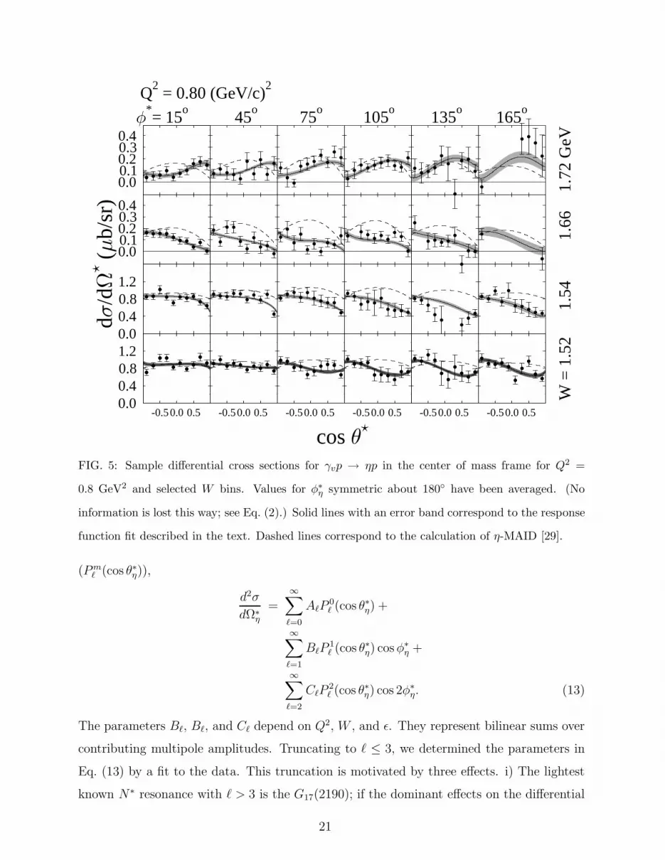
Results from this experiment are tabulated in the CLAS database [39]. For the Q2 = 0.8

GeV2 bin, Figure 5 shows sample cross sections for four W bins. The first two W bins,

W = 1.52 and 1.54 GeV are at the peak of the S11(1535) resonance. They show a dominant

19

TABLE IV: Binning details for the differential cross sections. For each Q2 bin, we show the

minimum and maximum values of Q2, the energy of the electron beam for the data set, the

maximum value of W probed, and the bin width in cos θ∗. The W bin widths in all cases were 20

MeV, while the φ∗ bins were 30 wide.

Q2min Q2

max Ebeam Wmax ∆ cos θ∗

(GeV2) (GeV2) (GeV) (GeV)

0.2 0.4 1.5 1.60 0.2

0.6 1.0 2.5 1.80 0.2

1.0 1.4 2.5 1.74 0.2

1.3 2.1 4.0 2.00 0.4

2.1 2.9 4.0 1.92 0.4

isotropic component due to the S11(1535) → ηp process, but deviations from isotropy can

be seen, especially at large φ∗. By W = 1.66 GeV, the non-isotropy is quite evident. The

cross section falls monotonically as a function of cos θ∗, with the cross section for forward

η production consistent with zero. As W increases this feature changes dramatically. At

W = 1.72 GeV, the forward-backward asymmetry of the distributions has reversed, with

forward η production favored, while backward production is close to zero.

The η-MAID model [29], based on the MAID formalism [30], has been developed for η

electro- and photoproduction. This is an isobar model using a relativistic Breit-Wigner W

dependence with form factors. Eight PDG 3* and 4* resonances of mass less than 1.8 GeV

and nonresonant processes are included at the amplitude level. They fit the photoproduction

data [11, 12, 42] and the Q2 dependence of the total cross section from electroproduction

data [19, 21] in the S11(1535) region. The results of a calculation implementing this model

are included in Figure 5. These calculations roughly match the observed cross sections.

However, the angular dependence predicted by η-MAID does not agree with our data at W

above the S11(1535) region. The model was not fit to the differential cross sections of our

previous work and the Q2 dependence of the higher mass resonances, e.g. D15(1675), was

taken from a quark model calculation rather than from data.

For each W and Q2 bin, the differential cross sections are fit to a form that comes from an

expansion of the response functions from Eq. (2) in terms of associated Legendre polynomials

20

cos

d/d

(b/

sr)

*= 15

o45

o75

o105

o135

o165

o

W=

1.52

1.54

1.66

1.72

GeV

Q2

= 0.80 (GeV/c)2

-0.50.0 0.50.00.40.81.2

-0.50.0 0.5 -0.50.0 0.5 -0.50.0 0.5 -0.50.0 0.5 -0.50.0 0.5

0.00.40.81.2

0.00.10.20.30.4

0.00.10.20.30.4

FIG. 5: Sample differential cross sections for γvp → ηp in the center of mass frame for Q2 =

0.8 GeV2 and selected W bins. Values for φ∗η symmetric about 180 have been averaged. (No

information is lost this way; see Eq. (2).) Solid lines with an error band correspond to the response

function fit described in the text. Dashed lines correspond to the calculation of η-MAID [29].

(P mℓ (cos θ∗η)),

d2σ

dΩ∗η

=∞∑

ℓ=0

AℓP0ℓ (cos θ∗η) +

∞∑

ℓ=1

BℓP1ℓ (cos θ∗η) cos φ∗

η +

∞∑

ℓ=2

CℓP2ℓ (cos θ∗η) cos 2φ∗

η. (13)

The parameters Bℓ, Bℓ, and Cℓ depend on Q2, W , and ǫ. They represent bilinear sums over

contributing multipole amplitudes. Truncating to ℓ ≤ 3, we determined the parameters in

Eq. (13) by a fit to the data. This truncation is motivated by three effects. i) The lightest

known N∗ resonance with ℓ > 3 is the G17(2190); if the dominant effects on the differential

21

cross section arise from interference with the dominant ℓ = 0 partial wave, terms above

l = 3 should be negligible. ii) Fits to the η-MAID predicted cross sections yield negligible

contributions for terms higher than ℓ = 3. iii) Good fits to the data are obtained with the

truncated sum.

FIG. 6: Results from fitting the angular distribution data of this experiment to Eq. (13). Coeffi-

cients of the φ∗ independent terms are shown, i.e. those that contribute to σT +ǫσL. Contributions

from both statistical and systematic sources are displayed. The dashed line is the η-MAID predic-

tion [29] and the solid line is a four resonance fit to these terms.

Results are shown versus W in Figures 6, 7, and 8. The quoted uncertainties contain

both statistical and systematic uncertainties. We repeated the fit taking into account shifts

in the cross section for each of the sources of systematic uncertainty studied in Section III.

The total systematic uncertainty on the extracted parameters is the sum in quadrature of all

22

FIG. 7: Same as Figure 6, but showing the parameters corresponding to σLT . For the four resonance

fit, these parameters are all zero.

individual sources. We normalize our fitted A1, A2, etc. to the isotropic term (A0) in order

to more clearly show the W and Q2 dependence of the shape of the differential cross section.

For the ratios the resulting uncertainty is dominated by the uncertainty on the numerators.

The isotropic component (A0 = σtot/4π) shows the same features as the angle-integrated

cross sections: a dominant peak from the S11(1535) with additional structure above W = 1.6

GeV. The other prominent term in the fit is A1, which represents the slope of the differential

cross section versus cos θ∗η. A structure in the W dependence of A1 was first seen in our

previous publication [21] and is also seen by the GRAAL photoproduction experiment [42].

By examining the ratio A1/A0 in the new data, we can study this structure in more detail.

Two features stand out in this ratio:

1. The ratio A1/A0 is large and makes a rapid change from negative to positive values at

W ≈ 1.7 GeV.

2. This structure is roughly independent of Q2 up to 2.5 GeV2.

23

FIG. 8: Same as Figure 6, but showing the parameters corresponding to σTT . For the four resonance

fit, these parameters are all zero.

The simplest description for A1 is in terms of interference between S and P waves. In that

case the rapid change in A1 between W = 1.66 and 1.72 GeV could be caused by one of the

waves passing through a resonance. There are 2 P -wave resonances in this region, P11(1710)

and P13(1720). The former is rated 3∗ by the PDG [9], but its properties are very difficult

to extract from data and is therefore controversial [43]. The latter is rated 4∗, but is also

poorly understood [10]. Fits to CLAS π+π− electroproduction data [23] provided evidence

that the existing baryon structure at W ∼ 1.7 GeV should be changed. Their fits prefer

either a greatly reduced ρN decay branch for the existing P13(1720) resonance or a new 32

+

state. In the present data, we cannot couple to a T = 3/2 state and are unable to distinguish

between P11 and P13 states; we choose to use only a P11 state. If one describes the cross

section using only S11 and P11 partial waves,

A1

A0=

2ℜ(E∗0+M1−)

|E0+|2 + |M1−|2. (14)

In this case, the rapid shift from backward to forward peaked cross sections would be due to

a rapid change in the relative phase of the E0+ and M1− multipoles because one of them is

passing through resonance. The observation that this structure in A1/A0 is approximately Q2

independent would then imply that S11 and P11 partial waves have a similar Q2 dependence.

The values of Bℓ shown in Fig. 7 are consistent with zero. These parameters measure

24

the σLT component of dσdΩ

, indicating that longitudinal amplitudes are not significant for this

reaction (as was assumed in Section IVA). The Cl parameters in Fig. 8 measure the σTT

component of dσdΩ

. They are small indicating the A3/2 components are also small for these

values of Q2.

To better understand the content of the η-MAID model, we also fit the parameters in

Eq. (13) to the predicted cross sections from that model. The extracted parameters are also

included in Figures 6, 7, and 8 as dashed lines. The prediction has a broader S11 peak than

is seen in our data. Some structure is predicted in A1 arising from the P11(1710), but the

size of this effect is not nearly enough to match our data. At high W , η-MAID predicts a

negative A1 in contrast to the significant positive value we observe. The model value of bηN

for P11(1710) is much larger than the PDG value. Our data indicates the model value is

incorrect. η-MAID contains many sources of D-wave contributions: D13(1520), D13(1700),

and D15(1675) in addition to nonresonant amplitudes. This produces a value for A2/A0 that

matches our data for W < 1.6 GeV, where the D13(1520) is the leading contribution. At

larger W , agreement is poor. The model value of bηN for D15(1675) is much larger than the

PDG value; our data indicates this is incorrect. The prediction for A3/A0 is near zero, as

are our measurements.

Predictions for the σLT and σTT terms are consistent with our measurements. C2 is the

only term that is not negligible in η-MAID for our values of Q2. It arises from the A3/2

amplitudes of the D-wave resonances interfering with the larger S-wave amplitude. Our

data agrees with this general trend, but the effect is small compared to the uncertainties.

To gain further understanding of the resonance content of our data, we did an additional

fit to the differential cross section data using relativistic Breit-Wigner resonances according

to Eqs. (7)-(10). We fit the extracted parameters, up to W = 1.8 GeV, to a sum of four

amplitudes for the following resonances: S11(1525), S11(1650), P11(1710), and D13(1520).

This set of resonances was determined empirically as the minimal set required to fit the

general features of our data. Although the properties of P11(1710) are very uncertain, it is

an important contributor to this fit. We label it as P11, but we cannot distinguish between

P11 and P13(1720) in our data set; specifically, a P13 resonance would also give a rapid

energy dependence in either A2 or C2 which we are unable to exclude with current statistical

accuracy. Only the transverse response function, σT is modeled, i.e. the Ai parameters. For

the resonances with small contributions (S11(1650) and D13(1520)), we fixed the resonance

25

parameters to values obtained elsewhere. Masses and widths were set to average values

from the Particle Data Group. For the D13(1520) we used the Q2 dependence of η-MAID.

Following the assumption of the single quark transition model [44], the ratio of the strength

of the S11(1650) to that of the S11(1535) was taken to be independent of Q2. Motivated

by the Q2 independence of A1/A0 in our data, we assumed the P11(1710) had the same Q2

dependence as the S11 states. This left 12 variables in the fit: the masses and widths of

the S11(1535) and P11(1710), the relative strengths of the S11(1650) and P11(1710) to that

of the S11(1535), an overall strength of the D13(1520), and the absolute strength of the

S11(1535) in each of the five Q2 bins. We view this as a simple fit. Our results should not be

interpreted as a precise determination of resonance parameters, but rather as an indication

of the dominant components needed in any future theoretical work.

The results of this fit are also shown in Figure 6. The fit yields a reasonable, though

not perfect description of our data. The isotropic term A0 is described by the dominant

S11(1535) peak, modified by the smaller S11(1650). The deviation from a simple Breit-

Wigner is described as a combination of destructive interference between the S11(1535) and

S11(1650), and a small contribution from the P11(1710). Including the S11(1650) results in

an extracted value of A 1

2

for the S11(1535) which is 7% higher than that obtained with a

single Breit-Wigner. The fitted width of the P11(1710) is 100 MeV, which is consistent with

the central (but very uncertain) PDG value. We cannot isolate the P11(1710) photocoupling

from that state’s branching ratio into ηp; we can only quote a ratio of ξ values (Eq. (6)).

The extracted value of ξ1710/ξ1535 is 0.22, which is about twice as large as in η-MAID, and

nearly an order of magnitude larger than that extracted from parameters of the P11(1710) in

the PDG. The D13(1520) primarily effects the quadratic term A2. Including this resonance

is enough to give a reasonable description of the W dependence of A2. Our data do not

require significant contributions from higher D-wave states present in the η-MAID model.

We fit the structure in A1/A0 with a smooth S-wave and a rapidly changing P -wave.

One could also describe this structure in terms of a new S-wave resonance interfering with

P -wave component as in the model of Saghai and Li [45]. However, the amplitudes for the

new resonance and the P -wave component must both fall off slowly with Q2 to reproduce

the data.

We also fit the φ dependence of the differential cross sections directly to Eq. (2) in order

to obtain σT + ǫσL, σLT , and σTT as a function of W , Q2 and cos θ∗. We choose to fit

26

the φ∗ dependence in terms of the parallel/perpendicular asymmetry (AsymTT ) and the

parallel/anti-parallel asymmetry (AsymLT ).

AsymTT =σ|| − σ⊥

σ|| + σ⊥

, (15)

where

σ|| =1

2(σ(φ = 0) + σ(φ = π)) (16)

and

σ⊥ =1

2(σ(φ = π/2) + σ(φ = 3π/2)) . (17)

AsymLT =σ(φ = 0) − σ(φ = π)

σ(φ = 0) + σ(φ = π). (18)

FIG. 9: Extracted values for σT + ǫσL, AsymLT , and AsymLT as a function of cos θ∗ for four

selected W bins with Q2 = 0.8 GeV2.

27

For photoproduction, σL and σLT don’t contribute. A common polarization parameter

is the parallel/perpendicular asymmetry, Σ. It is defined by AsymTT = ǫΣ; note also that

Σ = σTT /σT . In electroproduction, the possible presence of a longitudinal term makes the

relationships more complicated:

AsymTT =ǫσTT

σT + ǫσL(19)

AsymLT =

√

2ǫ(ǫ + 1)σLT

σT + ǫσL + ǫσTT. (20)

The data was analyzed in terms of these 3 response function combinations. A treatment

of systematic uncertainties similar to that used for differential cross sections was applied.

Figure 9 shows the values extracted from these fits for the same W and Q2 shown in Figure

5. Error bars display the systematic and statistical uncertainties. The quantity σT + ǫσL,

shows the same features we have discussed earlier. The values for AsymTT are consistent

with zero in all distributions, but the size of the estimated error bars are a strong function of

W . For W > 1.6, the total cross section is smaller than where the S11 resonance dominates.

Extraction of meaningful values for the φ dependence in this manner is therefore difficult.

V. CONCLUSIONS

Our extractions of A 1

2

for the excitation of the S11(1535) cover a large range and match

up well with Armstrong’s results [19] at higher Q2. It should be noted again that there

are significant model dependencies on describing the mass, width and branching ratio into

ηp. These uncertainties lead to significant systematic uncertainties on the absolute scale of

A 1

2

. These uncertainties are common to all points currently determined, so the shape of the

distribution is well determined. It becomes a significant challenge for theory to reproduce

this shape. No existing model is able to describe the full range.

Knowledge of the N∗ resonances in the region W ∼ 1700 MeV is presently weak because

the quality of older πN → ππN and πN → ηN data is poor. The coupling of known

P -wave resonances to ηN is thought to be very small. In this experiment, rapid energy

dependence in the strength in the P -wave for coupling to ηN final states is found. With

a simple resonance model, we are able to describe these data with significant coupling of a

P -wave resonance to ηN . As with S11(1535), the falloff of this coupling must be very slow.

28

Although we can describe our measurements in terms of the P11(1710), we cannot dis-

tinguish between that or the P13(1720) with these data . Either resonance could produce

the effect seen in A1/A0. The P11(1710) is more poorly understood than the P13(1720), so

it is easier to accommodate our data by altering the partial widths of the P11 rather than

the P13. A large P13 could also produce effects in other terms. For instance, interference

with a D-wave, would give a small contribution to A 3

2

, but not significant compared to

our uncertainties. A P13 resonance would have an A 3

2

photo-excitation as well as A 1

2

. Our

determination of A1/A0 is sensitive to the A 1

2

amplitude; a significant A 3

2

amplitude could

also lead to large effects in σTT .

Evidence for possible alterations in N∗ P -wave resonances at masses about 1.7 GeV is

accumulating. In addition to what is found in this experiment, double-pion production

experiments in this same mass range [23, 46] are also unable to be described with models

using existing information. Since different models are used to describe the different data

sets, it is important to use a common model to describe the combined measurements from

these (and other) reactions. Such a program may allow us to accurately determine the

properties of the P -wave resonances in this region.

VI. ACKNOWLEDGMENTS

We acknowledge the outstanding efforts of the staff of the Accelerator and the Physics

Divisions at JLab that made this experiment possible. This work was supported in part

by the U.S. Department of Energy, the National Science Foundation, the Istituto Nationale

di Fisica Nucleare, the French Centre National de la Recherche Scientifique, the French

Commissariat a l’Energie Atomique, and the Korea Science and Engineering Foundation.

Jefferson Science Associates (JSA) operates the Thomas Jefferson Science Facility for the

United States Department of Energy under contract DE-AC05-06OR23177.

[1] W. Konen and H. J. Weber, Phys. Rev. D 41, 2201 (1990).

[2] S. Capstick and B. D. Keister, Phys. Rev. D 51, 3598 (1995).

[3] F. E. Close and Z.-P. Li, Phys. Rev. D 42, 2194 (1990).

29

[4] C. Alexandrou, P. de Forcand, H. Neff, J. Negele, W. Schroers, and A. Tsapalis, Phys. Rev.

Lett. 94, 021601 (2005).

[5] J. M. Zanotti, D. B. Leinweber, A. G. Williams, and J. B. Zhang, Nucl. Phys. Proc. Suppl.

129, 287 (2004).

[6] S. Basak et al. (2006), ArXiv:hep-lat/0609072.

[7] B. Krusche and S. Schadmand, Prog. Part. Nucl. Phys. 51, 399 (2003).

[8] V. D. Burkert and T. S. H. Lee, Int. J. Mod. Phys. E 13, 1035 (2004).

[9] W.-M. Yao, C. Amsler, D. Asner, R. Barnett, J. Beringer, P. Burchat, C. Carone, C. Caso,

O. Dahl, G. D’Ambrosio, et al., Journal of Physics G 33, 1 (2006).

[10] T. P. Vrana, S. A. Dytman, and T. S. H. Lee, Phys. Rept. 328, 181 (2000).

[11] B. Krusche, et al., Phys. Rev. Lett. 74, 3736 (1995).

[12] J. Ajaka, et al., Phys. Rev. Lett. 81, 1797 (1998).

[13] P. S. Kummer, et al., Phys. Rev. Lett. 30, 873 (1973).

[14] U. Beck et al., Phys. Lett. B 51, 103 (1974).

[15] J. C. Alder, et al., Nucl. Phys. B 91, 386 (1975).

[16] F. W. Brasse et al., Nucl. Phys. B 139, 37 (1978).

[17] H. Breuker et al., Phys. Lett. B 74, 409 (1978).

[18] F. W. Brasse et al., Z. Phys. C 22, 33 (1984).

[19] C. S. Armstrong et al. (Jefferson Lab E94014), Phys. Rev. D 60, 052004 (1999).

[20] M. Ungaro et al. (CLAS Collaboration), Phys. Rev, Lett 97, 112003 (2006).

[21] R. Thompson et al. (CLAS Collaboration), Phys. Rev. Lett. 86, 1702 (2001).

[22] B. A. Mecking et al. (CLAS Collaboration), Nucl. Instrum. Meth. A 503, 513 (2003).

[23] M. Ripani et al. (CLAS Collaboration), Phys. Rev. Lett. 91, 022002 (2003).

[24] V. Crede et al. (CB-ELSA Collaboration), Phys. Rev. Lett. 94, 012004 (2002).

[25] L. N. Hand, Phys. Rev. 129, 1834 (1963).

[26] G. Chew, M. Goldberger, F. Low, and Y. Nambu, Phys. Rev. 106, 1345 (1957).

[27] T. Trippe et al. (Particle Data Group), Rev. Mod. Phys. 48, S157 (1976).

[28] R. Arndt, W. Briscoe, I. Strakovsky, and R. Workman, Phys. Rev. C 66, 055213 (1990).

[29] W.-T. Chiang, S.-N. Yang, L. Tiator, and D. Drechsel, Nucl. Phys. A 700, 429 (2002).

[30] D. Drechsel, O. Hanstein, S. S. Kamalov, and L. Tiator, Nucl. Phys. A 645, 145 (1999).

[31] M. Dugger et al. (CLAS Collaboration), Phys. Rev. Lett. 89, 222002 (2002).

30

[32] M. Benmerrouche, N. C. Mukhopadhyay, and J. F. Zhang, Phys. Rev. D 51, 3237 (1995).

[33] B. Krusche, N. Mukhopadhyay, J. Zhang, and M. Benmerrouche, Phys. Lett. B 397, 171

(1997).

[34] G. Knochlein, D. Drechsel, and L. Tiator, Z. Phys. A 352, 327 (1995).

[35] J. Blatt and V. Weisskopf, Theoretical Nuclear Physics (Dover, 1991).

[36] R. Ent, B. Fillipone, N. Makins, R. Milner, T. O’Neill, and D. Wasson, Phys. Rev. C 64,

054610 (2001).

[37] L. Mo and Y. Tsai, Rev. Mod. Phys. 41, 205 (1969).

[38] GEANT Detector Description and Simulation Tool, CERN, Geneva, w5013 ed. (1993).

[39] physics database of CLAS collaboration, http://clasweb.jlab.org/physicsdb.

[40] M. Aiello, M. M. Giannini, and E. Santopinto, J. Phys. G 24, 753 (1998).

[41] I. Aznauryan, V. Burkert, G. Fedotov, B. Ishkhanov, and V. Mokeev, Phys. Rev. C 72, 045201

(2005).

[42] F. Renard et al. (GRAAL Collaboration), Phys. Lett. B 528, 215 (2002).

[43] R. Arndt, Y. Azimov, M. Polyakov, I. Strakovsky, and R. Workman, Phys. Rev. C 69, 035208

(2004).

[44] A. Hey and J. Weyers, Phys. Lett. B 48, 69 (1974).

[45] B. Saghai and Z.-P. Li, Eur. Phys. J. A 11, 217 (2001).

[46] Y. Assafiri et al., Phys. Rev. Lett. 90, 222001 (2003).

31