Elevation dependency of mountain snow depth

TCD4, 1–30, 2010

Variability of snowdepth and SWE in a

small mountaincatchment

T. Grunewald et al.

Title Page

Abstract Introduction

Conclusions References

Tables Figures

J I

J I

Back Close

Full Screen / Esc

Printer-friendly Version

Interactive Discussion

The Cryosphere Discuss., 4, 1–30, 2010www.the-cryosphere-discuss.net/4/1/2010/© Author(s) 2010. This work is distributed underthe Creative Commons Attribution 3.0 License.

The CryosphereDiscussions

This discussion paper is/has been under review for the journal The Cryosphere (TC).Please refer to the corresponding final paper in TC if available.

Spatial and temporal variability of snowdepth and SWE in a small mountaincatchmentT. Grunewald, M. Schirmer, R. Mott, and M. Lehning

WSL Institute for Snow and Avalanche Research SLF, 7260 Davos Dorf, Switzerland

Received: 22 December 2009 – Accepted: 23 December 2009 – Published: 13 January 2010

Correspondence to: T. Grunewald ([email protected])

Published by Copernicus Publications on behalf of the European Geosciences Union.

1

http://www.the-cryosphere-discuss.net

http://www.the-cryosphere-discuss.net/4/1/2010/tcd-4-1-2010-print.pdf

http://www.the-cryosphere-discuss.net/4/1/2010/tcd-4-1-2010-discussion.html

http://creativecommons.org/licenses/by/3.0/

TCD4, 1–30, 2010



T. Grunewald et al.

Title Page



Tables Figures

J I

J I

Back Close

Full Screen / Esc



Abstract

The spatio-temporal variability of the mountain snow cover determines the avalanchedanger, snow water storage, permafrost distribution and the local distribution of faunaand flora. Using a new type of terrestrial laser scanner (TLS), which is particularlysuited for measurements of snow covered surfaces, snow depth, snow water equiv-5

alent (SWE) and melt rates have been monitored in a high alpine catchment duringan ablation period. This allowed for the first time to get a high resolution (2.5 m cellsize) picture of spatial variability and its temporal development. A very high variabilityin which maximum snow depths between 0–9 m at the end of the accumulation seasonwas found. This variability decreased during the ablation phase, although the domi-10

nant snow deposition features remained intact. The spatial patterns of calculated SWEwere found to be similar to snow depth. Average daily melt rate was between 15 mm/dat the beginning of the ablation period and 30 mm/d at the end. The spatial variationof melt rates increased during the ablation rate and could not be explained in a simplemanner by geographical or meteorological parameters, which suggests significant lat-15

eral energy fluxes contributing to observed melt. It could be qualitatively shown that theeffect of the lateral energy transport must increase as the fraction of snow free surfacesincreases during the ablation period.

1 Introduction

The largest part of annual winter-precipitation in the Alps above 1000 m a.s.l. falls as20

snow and most of it is stored for the season in the snow cover. When snow melt startsat the end of the accumulation season, the water is returned to the hydrologic cycle.Amount and timing of the melt strongly depend on thickness and spatial distribution ofthe snow cover. Hence the spatial and temporal variability of the snow cover has a highimpact on the alpine water balance and strongly affects nature and mankind (Elder et25

al., 1998). For instance, the supply with drinking water and energy, agriculture and

2





TCD4, 1–30, 2010



T. Grunewald et al.

Title Page



Tables Figures

J I

J I

Back Close

Full Screen / Esc



vegetation growth, all strongly depend on snow cover and alpine water storage (e.g.Armstrong and Brown, 2008; Jones et al., 2001; Keller et al., 2000). On the other hand,rapid melting can cause flooding and increased erosion (e.g. Pomeroy and Gray, 1995;Male and Gray, 1981). Furthermore, winter tourism with its high economic importancein many alpine regions, strongly depends on snow reliability and snow cover duration5

(e.g. Beniston, 2000; Haefner et al., 1997; Lopez-Moreno and Nogues-Bravo, 2006;Fazzini et al., 2004; Marty, 2008).

To make reliable assessments of current and future snow dynamics, it is essential toobtain a better understanding of the total amount of snow stored in a catchment andhow snow cover changes in space and time, especially in the ablation period.10

A lot of work has been carried out on the spatial variability of snow depth and snowwater equivalent (SWE) and how it is influenced by meteorological and topographicalfactors on different scales (e.g. Bloschl, 1999; Merz et al., 2009; Liston and Sturm,2002; Balk and Elder, 2000; Pomeroy et al., 2003; Deems et al., 2006; Trujillo et al.,2007; Mott et al., 2008; Dadic et al., 2010). In particular, snow deposition and snow15

transport due to wind have been investigated in much detail (e.g. Doorschot et al.,2001; Lehning et al., 2008) and it has been shown that snow distribution influencesrunoff dynamics in mountain catchments (Lehning et al., 2006). Many of these efforts,however, are based on model studies and suffer from insufficient validation againstmeasurements. Very often, limited snow depth and SWE observations are extrapolated20

to large areas using statistical models (e.g. Lopez-Moreno and Nogues-Bravo, 2006;Marchand and Killingtveit, 2004; Chang and Li, 2000; Luce et al., 1999; Erickson et al.,2005).

A promising attempt to gain area-wide high resolution snow depth data is the intro-duction of lidar altimetry to snow sciences. Airborne laser scanning (ALS) was proofed25

to be an appropriate and accurate method for gathering area-wide snow depth mea-surements (Deems and Painter, 2006; Hopkinson et al., 2001). ALS data was used toinvestigate spatial variability and scale invariance of snow depth and its relationship towind direction, vegetation and topography for several mountainous test sites (Deems

3





TCD4, 1–30, 2010



T. Grunewald et al.

Title Page



Tables Figures

J I

J I

Back Close

Full Screen / Esc



et al., 2006; Trujillo et al., 2007).In recent years, the introduction of terrestrial laser scanning (TLS) to snow science

has given a further push forwards as this technology provides the possibility to domore cost effective and flexible area-wide snow depth observations with high spatialresolution (Bauer and Paar, 2004; Jorg et al., 2006; Prokop, 2008). Prokop et al. (2008)5

and Schaffhauser et al. (2008) performed detailed investigations on the accuracy ofTLS for measuring snow depth. Both studies arrive at the conclusion that TLS is anappropriate tool for mapping snow depth with high accuracy.

However, no studies exist which use this promising technique to focus on snowdepth and SWE distribution and their time development for a catchment. By per-10

forming repeated TLS measurement campaigns in the Albertibach-catchment (Davos,Switzerland) for the whole ablation season of winter 2007/08, we present a uniquedata set of snow depth and SWE variability in a high mountain setting: the repeatedcatchment-wide measurement campaigns offer the possibility to investigate seasonalsnow cover changes by looking at snow depth changes (mostly depletion) during the15

ablation phase.This paper presents a first qualitative and quantitative investigation of this unique

dataset. We first give an overview on the study site and the methods used for collecting,processing and analysing the data in the method and data section. Then a section onresults and discussion of the data and findings is given before ending the paper with20

a conclusion of the main results of the study and a short outlook on future tasks andchallenges.

2 Method and data

2.1 Site description

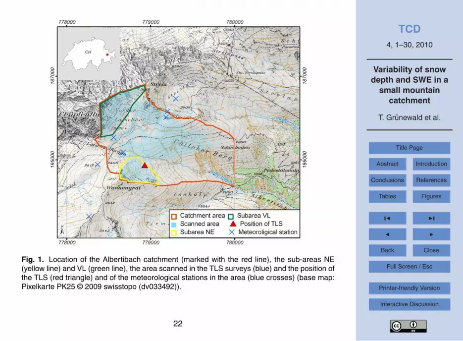
The area of investigation is a small high mountain catchment located in the region of25

Davos (Switzerland) (Fig. 1). The area of interest is defined by the drainage area of

4





TCD4, 1–30, 2010



T. Grunewald et al.

Title Page



Tables Figures

J I

J I

Back Close

Full Screen / Esc



the Albertibach, which discharges in an easterly direction and is surrounded by steepmountain ridges to the North and South. The elevation of the area ranges from 1940to 2658 m a.s.l. and is located above the local tree line. The total size of the catchmentarea is 1.3 km2, of which we covered 0.6 km2 (46%) in the laser surveys. The scannedarea can be regarded as representative for the whole catchment in terms of elevation5

range, aspect, and slope.The site is well equipped with a dense network of seven meteorological stations,

which provide a continuous series of meteorological data.

2.2 Measurement methodology and accuracy assessment

We carried out four measuring campaigns to collect the data used in this study in10

winter 2007/08. The first survey was made at the end of the accumulation season(26 April 2008) and we continued at intervals of about two weeks until the end of themelting season (13 May, 2 June and 10 June 2008).

To investigate area wide snow depth, we used a Riegl LPM 321 terrestrial laser scan-ner (Riegl, 2008). With a wavelength of 905 nm, the LPM 321 operates in a wavelength15

where the reflectivity of snow is very high. As the maximal distances we measuredwere below 1000 m, it was possible to scan in the LPM ’s near range mode (up to1500 m), which provides the best spatial resolution and accuracy. Detailed informationhow to measure snow depth with TLS can be found in Prokop (2008).

We subjected all laser data to a variety of quality checks, in particular, we compared20

the laser measurements with measurements obtained from a tachymeter, as describedin Prokop et al. (2008). The quality control revealed that snow depths showed meandeviations in z-direction of less than 4 cm and standard deviations of less then 5 cmat distances of up to 250 m. This is a higher level of accuracy than that publishedby Prokop et al. (2008) and more than sufficient for our purposes. Furthermore, an25

airborne laser scan (ALS) is available for the end of the accumulation season usingan independent helicopter based technology (Skaloud et al., 2006; Vallet et al., 2005).With this data, it was possible to investigate whether there are systematic errors in the

5





TCD4, 1–30, 2010



T. Grunewald et al.

Title Page



Tables Figures

J I

J I

Back Close

Full Screen / Esc



terrestrial scans. The analysis showed that the ALS had a mean deviation of less than5 cm against the tachymeter survey, which took place at the same time. The standarddeviation was 6 cm. The spatial distribution of the deviation in z-direction between theALS and the TLS survey for 26 April is shown in Fig. 2. Comparing TLS and ALS gavea mean deviation of 10 cm and a standard deviation of 13 cm. The difference between5

TLS and ALS increased with the distance measured by the TLS as is clearly visiblein Fig. 2 (blue colours). This might be due to the TLS being less accurate over longdistances but the accuracy is still more than sufficient for the analysis presented here.

2.3 Data processing

TLS does not measure snow depth directly but the point distances from the scanner to10

the surface of the targets (snow surface) with high spatial resolution and accuracy. Toget absolute snow depths, the scans must be subtracted from a digital elevation model(DEM). The DEM used in this study was created from a summer TLS survey using thesame technology.

We produced raster maps of snow depth data with a cell size of 2.5 m for each15

survey. Furthermore, we calculated the average daily snow depth change between twosucceeding surveys for every raster cell. To avoid erroneous daily snow depth changesfor pixels which showed a complete melt out before the later survey, we removed thosecells from the analysis. This was done by creating a binary raster mask from the colourinformation in the orthophotos, which were also taken during the TLS surveys. These20

masks were then applied to maps of snow depth and snow depth change which areanalyzed below.

To calculate SWE from snow depth data, average snow cover density estimationsare necessary. Many studies have found that the spatial variability of SWE is rela-tively small in comparison to snow depth (e.g. Pomeroy and Gray, 1995; Marchand and25

Killingtveit, 2004; Dickinson and Whiteley, 1971). Consequently, it is common to esti-mate areal SWE with a small number of representative density measurements and ahigh number of snow depth data (e.g. Rovansek et al., 1993; Elder et al., 1998; Jonas

6





TCD4, 1–30, 2010



T. Grunewald et al.

Title Page



Tables Figures

J I

J I

Back Close

Full Screen / Esc



et al., 2009). Thus, we calculated SWE based on a small number of well selected den-sity measurements. Depth-average snow density is often assumed to be controlled bya small number of topographical and meteorological parameters which are total snowdepth, elevation, solar radiation, climatic region and vegetation patterns (e.g. Jonaset al., 2009; Anderton et al., 2004). Because of the limited extent of the investigation5

area, we only focus on snow depth and solar radiation in this study.To ascertain wether there was a significant dependency between the snow den-

sity (ρ) and solar radiation, we classified the investigation area into three sub-areasusing total potential incoming solar radiation for the particular time periods betweentwo investigations, as simulated with the physical based model Alpine3D (Lehning10

et al., 2006; Helbig et al., 2009). For each radiation class, we took three manualSWE-measurements at locations with different snow depths (HS) (<50 m, 50–100 cm,>120 cm). Thus we obtained a depth dependent average density, ρ(R,t), for each ra-diation class (R) and each time step (t). To test the significance of the dependenciesρ(R) and ρt we used the Kruskal-Wallis test. The tests showed that there were sig-15

nificant differences for the specific time steps ρ(t) but no significant dependency onradiation class ρ(R) could be found. We also investigated if a direct relationship be-tween HS and ρ(t) was obvious from the measurements but no general trend could befound. We hence decided to use a single ρ(t) for each time step which translates snowdepth to SWE:20

SWE = ρ(t)HS (1)

where SWE is in mm and HS in m. A summary of the calculated ρ(t) values are givenin Table 1.

As a next step, we produced maps with the total SWE using Eq. (1) and averagedaily “melt rate”, which is simply taking the SWE rate of change between consecutive25

laser scans. The so called melt rate can include contributions from snow falls, settling,snow transport, snow sublimation and true melting. As the SWE maps are the resultsof a simple linear relationship as given in Eq. (1), the patterns of the snow depth maps

7





TCD4, 1–30, 2010



T. Grunewald et al.

Title Page



Tables Figures

J I

J I

Back Close

Full Screen / Esc



and the SWE maps are identical for each single time step. Hence we will focus ouranalysis on SWE-maps only and give the values for snow depth in brackets whereappropriate. Since ρ is time dependent, the melt rate and snow depth change mapsdid not show exactly the same patterns. But as there were no relevant differences inthe characteristic features we only show the results obtained from the daily melt rates5

in what follows.To refine the analysis, we separated two sub-areas from the investigation area

(Fig. 1) based on the visual impression that two different snow distribution patternsmay dominate these two sub-areas: the first covers the north-easterly exposed slopesof Wannengrat, and will be referred to as NE in the following. It is characterized by10

a highly variable snow deposition on a rather large scale. The second sub-area con-sists of the south-facing slopes of the Vordere Latschuel (VL), which appears to havea rather homogeneous snow distribution.

2.4 Data analysis

A quantitative analysis of the raster maps allowed a detailed evaluation of the spatial15

and temporal variability of SWE, on the one hand, and the average melt rates, on theother hand. We first visually interpreted the maps to identify obvious surface structuresand characteristics. To quantify the spatial variability and changes in time, histogramplots for the distribution of SWE and the average melt rates between the individualscans were examined. Furthermore, we investigated basic statistics such as mean20

(µ), standard deviation (σ) and total snow volume for each time period. As describedabove, the statistical parameters always refer to the snow-covered area. We then fo-cused on possible statistical dependencies of the melt rate in the investigation areaon topographic and meteorological parameters. For this purpose, the Pearson’s lin-ear correlation coefficient for the melt rate as dependent variable.was calculated. As25

independent variables we used:

– Topographical parameters derived from the DEM: altitude, slope, northing (differ-

8





TCD4, 1–30, 2010



T. Grunewald et al.

Title Page



Tables Figures

J I

J I

Back Close

Full Screen / Esc



ence in degrees from north).

– Mean daily sum of incoming solar radiation, simulated with the physical basedmodel Alpine3D (Lehning et al., 2006; Helbig et al., 2009), for each period of twosucceeding surveys. As input data for the model, we used data derived from anautomatic weather and snow station located in the catchment. The model then5

produced hourly output for incoming shortwave radiation for each grid-cell of a10 m-raster. We then averaged the output to one mean radiation day for each ofthe three periods.

– SWE at the end of the accumulation season (SWEmax) derived from TLS survey.

– Local windspeed obtained from high resolution flow fields; simulated with the10

mesoscale atmospheric model ARPS (Xue et al., 2000; Mott et al., 2008; Rader-schall et al., 2008; Mott and Lehning, 2010). The three-dimensional windspeedwas modelled on a horizontal grid resolution of 5 m. The local flow fields werecalculated for a north-westerly and a south-westerly wind situation, which wereobserved to be the predominant wind directions for the three periods between the15

scans. Note that for the first period both wind situations occurred but the north-westerly situation dominated. In contrast, in the second period, both prevailingwind direction occurred with a similar frequency. A major foehn event occurredin beginning of this period. In the third period only north-westerly wind situationswere observed.20

To account for possible interactions between these parameters, we combined the vari-ables mentioned above, in multiple linear regression models. Only the models whichperformed best will be shown in the following.

9





TCD4, 1–30, 2010



T. Grunewald et al.

Title Page



Tables Figures

J I

J I

Back Close

Full Screen / Esc



3 Results and discussion

3.1 Time development of SWE distribution

A map of the spatial SWE distribution in the investigation area for the end of the accu-mulation season (26 April) is shown in Fig. 3a. At that point of time, the whole catch-ment was snow covered, with exception of small snow-free patches in the steep rock5

faces in the south and north-west of the area. SWE averaged to 696 mm (HS 2.0 m)and peak SWE was 3120 mm (HS 9.0 m). Those exceptional large snow depths weremainly located at two cornice-like drifts which had formed at the steep north-easterlyexposed slopes of the Wannengrat summit due to drifting and blowing snow. Areas withabove average SWE could also be found in the steep south facing slopes of the Vordere10

Latschuel (VL). The flatter areas of the Chilcher Berg clearly showed average or belowaverage SWE. But line-like features with above average SWE were also clearly visiblein that area. From the DEM and a topographic map we could identify those featuresas ditches which were packed with snow probably due to snow transport processes(Lehning et al., 2008).15

The following scan, 17 days later, showed predominantly unchanged spatial patterns(Fig. 3b): the cross-slope accumulation zones in the NE remained the dominant featuretill the end of the ablation season while snow depth in the VL suffered stronger decreasethan average (Fig. 3c, d; see also Fig. 6). A significant number of snow-free patchesemerged especially on the knolls and ridges where SWE was lowest in the beginning of20

the ablation season. Complete melt out propagated quickly from those first snow-freeareas in the course of time. This may be because of lower snow depths at the edgesof the snow patches or because of lateral advective transport of heat from the warmersnow-free surfaces onto the colder snow cover (Essery and Pomeroy, 2004), which willbe discussed in detail below.25

Histogram representations of the distributions of SWE at the time of each scan areshown in Fig. 4. Mean snow depth was decreasing continuously (26 April=2.0 m,13 May=1.5 m , 2 June=1.3 m, 10 June=1.1 m) but mean SWE values remained on

10





TCD4, 1–30, 2010



T. Grunewald et al.

Title Page



Tables Figures

J I

J I

Back Close

Full Screen / Esc



a similar level for all time steps (26 April=697 mm, 13 May=569 mm , 2 June=570 mm,10 June=559 mm), which is interesting and counter-intuitive at first. This finding is, toa smaller degree, explained by the increasing snow densities (Table 1), which partlybalanced the effect of decreasing mean snow depth for the last three surveys. Theincrease in snow density can be explained by processes like settling, moisture pen-5

etration or melt – refreeze processes of the snow cover. More importantly, however,the snow covered area, to which the statistics are referring to, changed in time – thelater in the season, the smaller was the snow-covered area due to melt out of signif-icant portions of the catchment. Areas which only had a shallow snow cover at peakaccumulation were lowering the mean SWE at that time in comparison to the later sur-10

veys when those areas were bare and did no longer contribute to the statistics. Ananalysis of the statistics, which only include those raster cells which were still snowcovered in the last survey, confirmed this hypothesis: the mean SWE values werenow much higher at the peak of snow accumulation (Fig. 4b) and decreased with time(26 April=1248 mm, 13 May=1025 mm , 2 June=769 mm, 10 June=581 mm).15

This effect of snow density and snow covered area at the time of each scan wasalso visible in the standard deviation values (σ), which were used to quantify the spa-tial variability of the data: σ of snow depth, referring to the snow covered area, was1.3 m at the end of the accumulation season and decreased continuously (13 May=1.1,2 June=1.0) to 0.9 m at the end of the ablation season whereas σ-values for SWE20

(450–460 mm) remained similar until the last survey. Nevertheless, it can be seen thatthe spatial variability of both, snow depth and SWE was high for all time steps.

Figure 4b also shows that the histogram graphs for SWE are characterized by similarshape for all time steps and that the only change was a shift towards smaller values.This means that the variability of SWE remained constant while mean SWE decreased25

when only considering the areas which had not melted out completely at the time ofthe last survey. Looking again at the histogram graphs which contain the completearea, which was snow-covered at the time of the respective survey, clearly indicatesa different behaviour with a changing shape of the SWE distribution (Fig. 4a) as an

11





TCD4, 1–30, 2010



T. Grunewald et al.

Title Page



Tables Figures

J I

J I

Back Close

Full Screen / Esc



effect of the difference in snow-covered area. The decrease in snow-covered area hada major effect on the volume of SWE stored in the catchment, which was 3.3×105 m3

at 26 April and steadily depleted to 0.7×105 m3 at 10 June.Comparing the two sub-areas, VL and NE, clearly shows differences in the distribu-

tions of SWE (Fig. 5a, b). The cross-slope accumulation zones (discussed above)5

which featured the areas maximums SWE were located in NE. Mean SWE with1059 mm (HS=3.1 m) were therefore larger in the NE than in the VL with 919 mm(2.7 m) at the end of the accumulation season. A higher variability could also be ob-served in the NE (σ=569 mm/1.7 m) than in the VL (σ=335 mm /1.0 m) at the end offthe accumulation season. This finding is also obvious from Fig. 3, where the more10

homogenous snow depth values in the VL are clearly visible. The context of highervariability and higher mean SWE in the NE remained dominant during the whole abla-tion season.

3.2 Spatio-temporal variability of melt rates and their correlation with simpleweather and terrain parameters15

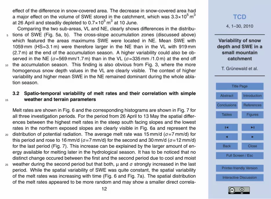
Melt rates are shown in Fig. 6 and the corresponding histograms are shown in Fig. 7 forall three investigation periods. For the period from 26 April to 13 May the spatial differ-ences between the highest melt rates in the steep south facing slopes and the lowestrates in the northern exposed slopes are clearly visible in Fig. 6a and represent thedistribution of potential radiation. The average melt rate was 15 mm/d (σ=7 mm/d) for20

this period and rose to 16 mm/d (σ=7 mm/d) for the second and 30 mm/d (σ=12 mm/d)for the last period (Fig. 7). This increase can be explained by the larger amount of en-ergy available for melting later in the hydrological season. It has to be noticed that nodistinct change occured between the first and the second period due to cool and moistweather during the second period but that both, µ and σ strongly increased in the last25

period. While the spatial variability of SWE was quite constant, the spatial variabilityof the melt rates was increasing with time (Fig. 6 and Fig. 7a). The spatial distributionof the melt rates appeared to be more random and may show a smaller direct correla-

12





TCD4, 1–30, 2010



T. Grunewald et al.

Title Page



Tables Figures

J I

J I

Back Close

Full Screen / Esc



tion with topographic factors. This temporal change in variability and spatial patternsmight be explained by a shift of the dominating processes which had an impact on themelting: in the first two periods, the energy available for melting was dominated byshortwave radiation which is also indicated by the relatively strong correlation coeffi-cient for shortwave radiation (r=0.3) described below. Later in the hydrological season5

the rapidly increasing fraction of snow free areas leads to changes in the energy bal-ance: the surface albedo of snow free patches is small and causes higher surfacetemperatures and higher values of lateral sensible heat fluxes and longwave radiation,which then lead to increased melting of the surrounding snow patches (Essery andPomeroy, 2004) especially at the edges of the patches. Thus, big differences in melt-10

ing between small and larger snow patches may occur. Nonetheless, a comparison ofcoefficient of variation values (CV=σ/µ) showed that the spatial variability of the meltrates with CV – values of 0.4–0.5 was lower than the spatial variability of snow depthand SWE (CV=0.6–0.8), even for the latest time period, where the scatter in melt rateswas largest. As can be seen in Fig. 3, as the consequence, the relatively low variabil-15

ity of the melt rates cannot substantially alter the spatial structure of SWE, which wasdetermined during the accumulation season. As an example, both pronounced accu-mulation zones in sub-area NE remained visible for the whole period of investigation.Thus, the effects of spatially variable melting on snow depletion are smaller than theeffect of the snow distribution at the end of the accumulation season. Snow remains20

there, where most snow was accumulated during the accumulation season. This inter-pretation is consistent to the findings of Anderton et al. (2004), who stated that spatialpatterns of snow disappearance were largely determined by the distribution of SWE atthe start of the melt season, rather than by spatial variability in melt rates during themelt season. Their results based on manual surveys are now confirmed by our more25

detailed dataset.Similar to the study of Anderton et al. (2004), we could only identify weak correla-

tions between the melt rates on the one hand, and the explanatory topographic andmeteorological parameters, on the other hand. Pearson’s linear correlation coefficients

13





TCD4, 1–30, 2010



T. Grunewald et al.

Title Page



Tables Figures

J I

J I

Back Close

Full Screen / Esc



are shown in Fig. 8 for all parameters and each time interval: altitude, slope, northing(each r=0.4), solar radiation (r=0.3) and windspeedSW (r=0.3) provided the best cor-relations for the first period (26 April–13 Mai). For the second period (13 May–2 June)all high correlations from the first period strongly decreased (slope: r=0.3, altitude, nor-thing each r=0.1, radiation r=0, windspeedSW=0.2) whereas SWEmax gave the best5

correlation with r=−0.4. In the final period (2 June–10 June) all correlations becamevery weak. This finding again suggests that the factors which dominate melt changein time. The strong decrease of the correlation is in this context attributed to the rais-ing heterogeneity of the surface and of its energy balance which we already describedabove. The later in the ablation season, the smaller the direct influence of the pa-10

rameters and the more “random” the melt pattern appears. It is important to note thatthe melt pattern is not really random but determined by the distribution of snow freepatches in the vicinity, which is not represented in local correlations. A further surpris-ing outcome is the decrease of the correlation coefficient for windspeedSW, althougha major foehn event occurred in the second period. Local high windspeeds promote15

turbulent fluxes and therefore affect the local energy balance. But advective effectsas discussed above would not show up in such a local analysis and require a moreinvolved analysis, which we plan to carry out in future.

The weak correlations become even more clearly when analysing the scatterplots ofthe melt rates against the predicting parameters. A scatter plot of melt rates against20

slope angle is shown in Fig. 9. The massive scattering of the data clearly illustratesthat high statiscical correlations can not be expected form these data.

These findings lead to the conclusion that none of the simple univariate parameterswas adequate to explain spatial melting characteristics in a satisfactory degree. Apossible additional factor other than lateral energy transport discussed above may be25

that the spatial resolution of 2.5 m, may still be too coarse. Windspeed was modelled ona spatial resolution of 5 m. A smaller horizontal resolution would strongly influence thelocal windspeed distribution (Mott and Lehning, 2010). Patterns which were causedby the micro-relief are not captured by that resolution. Furthermore, there may be

14





TCD4, 1–30, 2010



T. Grunewald et al.

Title Page



Tables Figures

J I

J I

Back Close

Full Screen / Esc



differences between the modelled meteorological variables and the true distribution,e.g. incoming radiation neglects frequent convective clouds over mountain tops.

To examine if interactions between the topographical and meteorological parame-ters might play a role, we built several multiple linear regression models, for which wetested different factor combinations. For the construction of the regression models, the5

variables were scaled linearly to [−1;1], to allow a direct comparison of the coefficients.Similar to the univariate correlation analysis, different models performed best for theindividual periods: the best fit for the first period is given in Eq. (2) and resulted in anr2 of 0.4. Additional factors and factor combinations could not significantly improve thefit.10

rate1 = 4.2 ·altitude+7.6 ·slope+5.6 ·northing+3.8 · radiation+12.2 (2)

For the second period an r2 of 0.3 was obtained from the model described in Eq. (3).Most variables which performed best in linear correlation analysis were also show-ing up in the multiple regression model, but in slightly different order. Slope was themost important variable in Eq. (2) and SWEmax accounted for the highest coefficient in15

Eq. (3).

rate2 =−2.1 ·altitude−8.8 ·slope−13.6 ·SWEmax+7.9 ·windspeedNW+18.2 (3)

The last period did not give remarkable correlations as discussed above. Like alreadyseen in the univariate correlations, we could observe a decrease in correlation withtime and this was confirmed by the multiple regressions. Therefore, the influence of20

topography and meteorology on melt rates gets consistently weaker later in the abla-tion season. Using f-test, all regressions were found to be highly significant (p<0.001)which is not surprising when taking the large size of the sample (N>18 000) into ac-count.

15





TCD4, 1–30, 2010



T. Grunewald et al.

Title Page



Tables Figures

J I

J I

Back Close

Full Screen / Esc



4 Conclusions

This contribution presents first results from a rich data set on the spatio-temporal vari-ability of snow depth. It is assumed that a high correlation between SWE and snowdepth (HS) allows a simple interpretation of snow depth in terms of SWE (Eq. 1) andtherefore most of the analysis is presented for calculated SWE maps and their tempo-5

ral changes, which are named “melt rate” maps although they are strictly the sum ofreal melt, sublimation and occasional smaller snowfalls.

Quality checks of the TLS measurement system against independent tachymeterand airborne laser scanning measurements have shown good accuracy of the snowdepth measurements such that the analysis presented appears not to be limited by10

measurement problems.A striking result from the analysis of SWE development during the ablation phase

is that a very variable distribution of “melt rates” is observed. We conclude that qual-itatively advective transport of melt energy from snow free areas to remaining snowpatches is a major source for this variability and leads to accelerated melt in the course15

of the ablation period in agreement with earlier results, which have been based on the-oretical considerations (Essery and Pomeroy, 2004). This conclusion is consistent withthe observation that initial weak correlations of melt rates with obvious meteorologicaland terrain parameters become even weaker towards the end of the ablation period.

Beyond the first analysis presented here, the data set allows significant further20

and more in depth work, which we are currently undertaking. A major effort is de-voted to a more quantitative understanding of lateral energy transport discussed aboveby using a combination of a meteorological with a detailed surface process model(ARPS/Alpine3D: Mott and Lehning, 2010). The most direct application is an assess-ment of total snow water storage as compared to interpolations made from flat field25

snow stations (e.g. Bocchiola et al., 2008; Janetti et al., 2008) and the validation ofsnow deposition and snow transport models (Lehning et al., 2008). A further interest-ing aspect is the development of surface roughness as a function of the variable snow

16





TCD4, 1–30, 2010



T. Grunewald et al.

Title Page



Tables Figures

J I

J I

Back Close

Full Screen / Esc



cover.

Acknowledgements. We thank all people who helped during the extensive field work and indata processing. Part of the work has been funded by the Swiss National Science Foundationand the European Community. This work would not have been possible without all colleaguesfrom SLF who contributed to this work in various ways.5

References

Anderton, S. P., White, S. M., and Alvera, B.: Evaluation of spatial variability in snow waterequivalent for a high mountain catchment, Hydrol. Process., 18, 435–453, 2004.

Armstrong, R. L. and Brown, R.: Introduction, in: Snow and climate, edited by: Armstrong, R.L. and Brun, E., Cambridge University Press, Cambridge, 1–11, 2008.10

Balk, B. and Elder, K.: Combining binary decision tree and geostatistical methods to estimatesnow distribution in a mountain watershed, Water Resour. Res., 36, 13–26, 2000.

Bauer, A. and Paar, G.: Monitoring von Schneehohen mittels terrestrischem Laserscanner zurRisikoanalyse von Lawinen, 14th International Course on Engineering Surveying, Zurich,15–19 March 2004.15

Beniston, M.: Environmental change in mountains and uplands, London UK and Oxford Uni-versity Press, New York, 2000.

Bloschl, G.: Scaling issues in snow hydrology, Hydrol. Process., 13, 2149–2175, 1999.Bocchiola, D., Bianchi Janetti, E., Gorni, E., Marty, C., and Sovilla, B.: Regional evaluation

of three day snow depth for avalanche hazard mapping in Switzerland, Nat. Hazards Earth20

Syst. Sci., 8, 685–705, 2008,http://www.nat-hazards-earth-syst-sci.net/8/685/2008/.

Chang, K. T. and Li, Z.: Modelling snow accumulation with a geographic information system,Int. J. Geogr. Inf. Sci., 14, 693–707, 2000.

Dadic, R., Mott, R., Lehning, M., and Burlando, P.: Wind influence on snow distribution and25

accumulation over glaciers, J. Geophys. Res., doi:10.1029/2009JF001261, in press, 2010.Deems, J. S., Fassnacht, S. R., and Elder, K. J.: Fractal distribution of snow depth from lidar

data, J. Hydromet., 7, 285–297, 2006.Deems, J. S. and Painter, T. H.: Lidar measurement of snow depth: Accuracy and error sources,

17





http://www.nat-hazards-earth-syst-sci.net/8/685/2008/

TCD4, 1–30, 2010



T. Grunewald et al.

Title Page



Tables Figures

J I

J I

Back Close

Full Screen / Esc



in: Proceedings of the International Snow Science Workshop ISSW, Telluride, CO, USA, 1–6October 2006, 384–391, 2006.

Doorschot, J., Raderschall, N., and Lehning, M.: Measurements and one-dimensional modelcalculations of snow transport over a mountain ridge, Ann. Glaciol., 32, 53–158, 2001.

Elder, K., Rosenthal, W., and Davis, R. E.: Estimating the spatial distribution of snow water5

equivalence in a montane watershed, Hydrol. Process., 12, 1793–1808, 1998.Erickson, T. A., Williams, M. W., and Winstral, A.: Persistence of topographic controls on the

spatial distribution of snow in rugged mountain terrain, Colorado, United States, Water Re-sour. Res., 41, W04014, doi:10.1029/2003WR002973, 2005.

Essery, R. and Pomeroy, J.: Implications of spatial distributions of snow mass and melt rate for10

snow-cover depletion: theoretical considerations, Ann. Glaciol., 38, 261–265, 2004.Fazzini, M., Fratianni, S., Biancotti, A., and Billi, P.: Skiability conditions in several skiing com-

plexes on Piedmontese and Dolomitic Alps, Meteorol. Z., 13, 253–258, 2004.Haefner, H., Seidel, K., and Ehrler, H.: Applications of snow cover mapping in high mountain

regions, Phys. Chem. Earth, 22, 275–278, 1997.15

Helbig, N., Lowe, H., and Lehning, M.: Radiosity approach for the shortwave surface radiationbalance in complex terrain, J. Atmos. Sci., 66, 2900–2912, 2009.

Hopkinson, C., Sitar, M., Chasmer, L., Gynan, C., Agro, D., Enter, R., Foster, J., Heels, N.,Hoffnan, C., Nillson, J., and St.Pierre, R.: Mapping the spatial distribution of snowpack depthbeneath a variable forest canopy using airborne laser altimetry, Proceedings of the 58th20

Eastern Snow Conference, 17–19 May 2001, Ottawa, Ontario, Canada, 2001.Janetti, E. B., Gorni, E., Sovilla, B., and Bocchiola, D.: Regional snow-depth estimates for

avalanche calculations using a two-dimensional model with snow entrainment, Ann. Glaciol.,49, 63–70, 2008.

Jonas, T., Marty, C., and Magnusson, J.: Estimating the snow water equivalent from snow depth25

measurements in the Swiss Alps, J. Hydrol., 378, 161–167, 2009.Jones, H. G., Pomeroy, J. W., Walker, D. A., and Hoham, R. W.: Snow ecology: An interdisci-

plinary examination of snow-covered ecosystems, Cambridge University Press, Cambridge,UK, 378 pp., 2001.

Jorg, P., Fromm, R., and Sailer, R. S. A.: Measuring snow depth with a terrestrial laser ranging30

system, Proceedings International Snow Science Workshop ISSW 2006, Telluride, CO, USA,1–6 October 2006, 452–460, 2006.

Keller, F., Kinast, F., and Beniston, M.: Evidence of the response of vegetation to environmental

18





TCD4, 1–30, 2010



T. Grunewald et al.

Title Page



Tables Figures

J I

J I

Back Close

Full Screen / Esc



change at high elevation sites in the Swiss Alps, Regional Env. Change, 1, 70–77, 2000.Lehning, M., Volksch, I., Gustafsson, D., Nguyen, T. A., Stahli, M., and Zappa, M.: Alpine3d: A

detailed model of mountain surface processes and its application to snow hydrology, Hydrol.Process., 20, 2111–2128, 2006.

Lehning, M., Lowe, H., Ryser, M., and Radschall, N.: Inhomogeneous precipitation5

distribution and snow transport in steep terrain, Water Resour. Res., 44, W07404,doi:10.1029/2007WR006545, 2008.

Liston, E. G. and Sturm, M.: Winter precipitation patterns in arctic Alaska determined from ablowing-snow model and snow-depth observations, J. Hydrometeorol., 3(4), 646–659, 2002.

Lopez-Moreno, J. I. and Nogues-Bravo, D.: Interpolating local snow depth data: An evaluation10

of methods, Hydrol. Process., 20, 2217–2232, 2006.Luce, C. H., Tarboton, D. G., and Cooley, K. R.: Sub-grid parameterization of snow distribution

for an energy and mass balance snow cover model, Hydrol. Process., 13, 1921–1933, 1999.Male, D. H. and Gray, D. M.: Snowcover ablation and runoff, in: Handbook of snow, edited by:

Gray, D. M. and Male, D. H., Pergamon Press, Toronto, CA, 360–436, 1981.15

Marchand, W. D. and Killingtveit, A.: Statistical properties of spatial snowcover in mountainouscatchments in Norway, Nord. Hydrol., 35, 101–117, 2004.

Marty, C.: Regime shift of snow days in Switzerland, Geophys. Res. Lett., 35, L12501,doi:10.1029/2008GL033998, 2008.

Merz, R., Parajka, J., and Bloschl, G.: Scale effects in conceptual hydrological modeling, Water20

Resour. Res., 45, W09405, doi:10.1029/2009WR007872, 2009.Mott, R., Faure, F., Lehning, M., Lowe, H., Hynek, B., Michlmayr, G., Prokop, A., and Schoner,

W.: Simulation of seasonal snow-cover distribution for glacierized sites on Sonnblick, Austria,with Alpine 3D model, Ann. Glaciol., 49, 155–160, 2008.

Mott, R. and Lehning, M.: Meteorological modelling of very high resolution wind fields and snow25

deposition for mountains, J. Hydromet., in review, 2010.Pomeroy, J. W. and Gray, D. M.: Snowcover accumulation, relocation and management, Saska-

toon, 1995.Pomeroy, J. W., Toth, B., Granger, R. J., Hedstrom, N. R., and Essery, R. L. H.: Variation

in surface energetics during snowmelt in a subarctic mountain catchment, J. Hydromet., 4,30

702–719, 2003.Prokop, A.: Assessing the applicability of terrestrial laser scanning for spatial snow depth mea-

surements, Cold Reg. Sci. Technol., 54, 155–163, 2008.

19





TCD4, 1–30, 2010



T. Grunewald et al.

Title Page



Tables Figures

J I

J I

Back Close

Full Screen / Esc



Prokop, A., Schirmer, M., Rub, M., Lehning, M., and Stocker, M.: A comparison of measure-ment methods: Terrestrial laser scanning, tachymetry and snow probing, for the determina-tion of spatial snow depth distribution on slopes, Ann. Glaciol., 49, 210–216, 2008.

Raderschall, N., Lehning, M., and Schar, M.: Fine-scale modeling of the bound-ary layer with wind field over steep topography, Water Resour. Res., 44, W09425,5

doi:10.1029/2007WR006545, 2008.Riegl Laser Measurement Systems, G.: Long-range laser profile measuring system LPM-321:

Technical documentation & user’s instructions, 2008.Rovansek, R. J., Kane, D. L., and Hinzman, L. D.: Improving estimates of snowpack water

equivalent using double sampling, Proceedings of the 61st Western Snow Conference, 8–1010

June 1993, Queebeck City, Canada, 1993.Schaffhauser, A., Fromm, R., Jorg, P., Luzi, G., Noferini, L., and Sailer, R.: Remote sensing

based retrieval of snow cover properties, Cold Reg. Sci. Technol., 54, 164–175, 2008.Skaloud, J., Vallet, J., Keller, K., Veyssiere, G., and Kolbl, O.: An eye for landscapes – rapid

aerial mapping with handheld sensors, GPS World, 17, 26–32, 2006.15

Trujillo, E., Ramirez, J. A., and Elder, K. J.: Topographic, meteorologic, and canopy controlson the scaling characteristics of the spatial distribution of snow depth fields, Water Resour.Res., 43, W07409, doi:10.1029/2006WR005317, 2007.

Vallet, J. and Skaloud, J.: Helimap: Digital imagery/lidar handheld airborne mapping systemfor natural hazard monitoring, 6 setmana Geomatica, Barcelona, 1–10 February 2005.20

Xue, M., Droegemeier, K. K., and Wong, V.: The advanced regional prediction system (ARPS)- a multi-scale nonhydrostatic atmospheric simulation model. Part I: Model dynamics andverification, Meteorol. Atmos. Phys., 75, 161–193, 2000.

20





TCD4, 1–30, 2010



T. Grunewald et al.

Title Page



Tables Figures

J I

J I

Back Close

Full Screen / Esc



Table 1. Depth-averaged snow density values ρ(t) kgm3 [kg/m2] for each time step.

26 Apr 13 May 2 Jun 10 Jun

ρ(t) 345.2 388.6 477.4 500.7

21





TCD4, 1–30, 2010



T. Grunewald et al.

Title Page



Tables Figures

J I

J I

Back Close

Full Screen / Esc



Copernicus Publications Bahnhofsallee 1e 37081 Göttingen Germany Martin Rasmussen (Managing Director) Nadine Deisel (Head of Production/Promotion)

Contact [email protected] http://publications.copernicus.org Phone +49-551-900339-50 Fax +49-551-900339-70

Legal Body Copernicus Gesellschaft mbH Based in Göttingen Registered in HRB 131 298 County Court Göttingen Tax Office FA Göttingen USt-IdNr. DE216566440

Page 1/1

Fig. 1. Location of the Albertibach catchment (marked with the red line), the sub-areas NE(yellow line) and VL (green line), the area scanned in the TLS surveys (blue) and the position ofthe TLS (red triangle) and of the meteorological stations in the area (blue crosses) (base map:Pixelkarte PK25 © 2009 swisstopo (dv033492)).

22





TCD4, 1–30, 2010



T. Grunewald et al.

Title Page



Tables Figures

J I

J I

Back Close

Full Screen / Esc



Fig. 2. Spatial distribution of the deviation in z-direction [m] between ALS and TLS survey for26 April 2008.

23





TCD4, 1–30, 2010



T. Grunewald et al.

Title Page



Tables Figures

J I

J I

Back Close

Full Screen / Esc



Fig. 3. SWE maps for 26 April (a), 13 May (c), 2 June (c) and 10 June (d). The black arrowsmark examples for snow filled ditches and cornice-like drifts (base map: Pixelkarte PK25 ©2009 swisstopo (dv033492)).

24





TCD4, 1–30, 2010



T. Grunewald et al.

Title Page



Tables Figures

J I

J I

Back Close

Full Screen / Esc



Fig. 4. Histograms of SWE for the snow covered area at the time of each scan (a) and for thosefractions only which had still snow at 10 June (b). Interval size: 63.

25





TCD4, 1–30, 2010



T. Grunewald et al.

Title Page



Tables Figures

J I

J I

Back Close

Full Screen / Esc



Fig. 5. Histograms of SWE for the sub-areas NE (a) and VL (b). Interval size for (a): 63, intervalsize for (b): 53.

26





TCD4, 1–30, 2010



T. Grunewald et al.

Title Page



Tables Figures

J I

J I

Back Close

Full Screen / Esc



Copernicus Publications Bahnhofsallee 1e 37081 Göttingen Germany Martin Rasmussen (Managing Director) Nadine Deisel (Head of Production/Promotion)

Contact [email protected] http://publications.copernicus.org Phone +49-551-900339-50 Fax +49-551-900339-70

Legal Body Copernicus Gesellschaft mbH Based in Göttingen Registered in HRB 131 298 County Court Göttingen Tax Office FA Göttingen USt-IdNr. DE216566440

Page 1/1

Fig. 6. Daily melt rates averaged for the time periods 26 April–13 May (a), 13 May–2 June (b)and 2 June–10 June (c) (base map: Pixelkarte PK25 © 2009 swisstopo (dv033492)).

27





TCD4, 1–30, 2010



T. Grunewald et al.

Title Page



Tables Figures

J I

J I

Back Close

Full Screen / Esc



Fig. 7. Histograms of daily melt rate for the whole catchment area. Interval size: 124.

28





TCD4, 1–30, 2010



T. Grunewald et al.

Title Page



Tables Figures

J I

J I

Back Close

Full Screen / Esc



Fig. 8. Coefficient of correlation (Pearson) for daily melt rates for each time period againstaltitude, slope, northing, SWE at the end of the accumulation season (SWEmax), incomingshortwave radiation for each period (ISWR) and windspeed for prevailing wind direction north-west (windspeedNW) and south-west (windspeedSW).

29





TCD4, 1–30, 2010



T. Grunewald et al.

Title Page



Tables Figures

J I

J I

Back Close

Full Screen / Esc



Fig. 9. Scatterplot of SWE melt rates (26 April–13 May) and slope angle. The solid line drawsthe linear fit function derived from the univariate regression analysis.

30





Documents

Elevation dependency of mountain snow depth