Seediscussions,stats,andauthorprofilesforthispublicationat:https://www.researchgate.net/publication/260285715

ElicitingSubjectiveProbabilitieswithBinaryLotteries

ARTICLEinJOURNALOFECONOMICBEHAVIOR&ORGANIZATION·MAY2014

ImpactFactor:1.01·DOI:10.1016/j.jebo.2014.02.011

CITATIONS

6

READS

35

3AUTHORS,INCLUDING:

GlennHarrison

GeorgiaStateUniversity

235PUBLICATIONS7,832CITATIONS

SEEPROFILE

JimmyMartinez-Correa

CopenhagenBusinessSchool

7PUBLICATIONS25CITATIONS

SEEPROFILE

Allin-textreferencesunderlinedinbluearelinkedtopublicationsonResearchGate,

lettingyouaccessandreadthemimmediately.

Availablefrom:JimmyMartinez-Correa

Retrievedon:05February2016

Eliciting Subjective Probabilities with Binary Lotteries

by

Glenn W. Harrisona, Jimmy Martínez-Correab,* and J. Todd Swarthoutc

Forthcoming Journal of Economic Behavior and Organization

February 2014

ABSTRACT.

We evaluate a binary lottery procedure for inducing risk neutral behavior in a subjective beliefelicitation task. Prior research has shown this procedure to robustly induce risk neutrality whensubjects are given a single risk task defined over objective probabilities. Drawing a sample from thesame subject population, we find evidence that the binary lottery procedure also induces linear utilityin a subjective probability elicitation task using the Quadratic Scoring Rule. We also show that thebinary lottery procedure can induce direct revelation of subjective probabilities in subjects withpopular Non-Expected Utility preference representations that satisfy weak conditions.

Keywords: Subjective probability elicitation, binary lottery procedure, experimental economics, riskneutrality

JEL classification: C81, C91.

† We are grateful for comments from two referees and participants at the Foundations and Applications of Utility, Riskand Decision Theory Conference, Georgia State University, Atlanta, 2012. We are also grateful to the Society ofActuaries and the Center for Actuarial Excellence Research Fund for financial support. Appendices are available inCEAR Working Paper 2012-09 at http://cear.gsu.edu.a Department of Risk Management & Insurance and Center for the Economic Analysis of Risk, Robinson College ofBusiness, Georgia State University, P.O. Box 4036, Atlanta, Georgia 30302-4036, USA. b Department of Economics, Copenhagen Business School, Porcelaenshaven 16A, 3.57, DK-2000 Frederiksberg,Denmark.c Department of Economics, Andrew Young School of Policy Studies, Georgia State University, P.O. Box 3992, Atlanta,Georgia, 30302-3992, USA.* Corresponding author. Tel.: + 45 3815 2349.E-mail addresses: gharrison@gsu.edu (G.W. Harrison), jima.eco@cbs.dk (J. Martínez-Correa) swarthout@gsu.edu (J. T.Swarthout).

The Quadratic Scoring Rule (QSR) directly elicits subjective probabilities so long as subjects

behave as if they are risk neutral. However, there is systematic evidence that subjects behave as if

they are risk averse, even when facing the relatively small stakes normally used in the laboratory. We

consider a procedure that should, theoretically, induce linear utility in applications of the QSR to

directly elicit subjective probabilities. Our controlled experiment leads us to conclude that this

procedure does indeed induce linear utility and accurately reveal latent subjective probabilities.

There are several ways to control for risk attitudes and recover underlying subjective

probabilities. Andersen et al. (2014) illustrate how one can jointly estimate risk attitudes and

subjective beliefs using a structural estimation approach.1 There also exist other mechanisms for

eliciting subjective probabilities without correcting for risk attitudes, such as the procedures

proposed by Grether (1992), Köszegi and Rabin (2008, p.199), Offerman et al. (2009), Karni (2009)

and Holt and Smith (2009).

We consider the use of proper scoring rules, such as the popular QSR, combined with a

Binary Lottery Procedure (BLP) to induce linear utility in subjects. Binary lottery procedures to

induce linear utility functions have a long history, with the major contributions being Smith (1961),

Roth and Malouf (1979) and Berg et al. (1986).2 The consensus appears to be that these procedures

may be fine in theory, but behaviorally they just do not work as advertized (e.g., Cox and Oaxaca,

1995, and Selten et al., 1999). However, Harrison et al. (2013) show that the BLP induces linear

utility over objective probabilities when contaminating factors such as strategic equilibrium concepts

and traditionally used payment protocols are avoided. They find that the BLP induces risk neutrality

when subjects are given one binary lottery choice over objective probabilities, and that it also works

1 The need to do this jointly is in fact central to the operational definition of subjective probabilityprovided by Savage (1954): under certain postulates, he showed that there existed a subjective probability anda utility function that could rationalize observed choices under subjective risk.

2 See Harrison et al. (2013) for a detailed discussion on the literature of the BLP.

-1-

well when subjects are given more than one binary choice.

Our goal is to determine whether the BLP induces risk neutrality in simple binary choices

defined over subjective probability elicitation tasks. We examine the ability of the QSR, combined with

the BLP, to directly elicit subjective probabilities without controlling for risk attitudes. The first

statements of this mechanism, joining the QSR and the BLP, appear to be Allen (1987) and

McKelvey and Page (1990).3 Schlag and ven der Weel (2013) and Hossain and Okui (2013) examine

the same extension of the QSR, along with certain generalizations, calling it a “randomized QSR”

and “binarized scoring rule,” respectively. Hossain and Okui (2013) test their theoretical results on

scoring rules and subjective probability elicitation with an experimental design that has the drawback

that they elicit beliefs about the composition of an urn that has probabilities that are objectively known

by the subjects. A proper test of the ability of BLP to recover subjective probabilities should involve

random processes that are not objectively known by subjects, and of course that provides a

methodological challenge since one must simultaneously control subjective probabilities about some

event and test if elicited responses are closer to these probabilities with the help of the BLP. Our

experimental design captures this critical feature.

Using non-parametric statistical tests we find evidence that the BLP mitigates the distortion

in reports introduced by risk aversion. Inferred subjective probabilities under the BLP robustly shift

in the direction predicted under the plausible, empirically supported assumption that subjects are

risk averse and that the BLP reduces the contaminating factor of risk aversion on optimal reports.

Structural econometric estimations provide further evidence consistent with the hypothesis that the

3 There is no shortage of theoretical procedures to elicit subjective probabilities, and one naturalquestion is which procedure generates them most reliably from a behavioral perspective. For example,Trautmann and van de Kuilen (2011) compare several incentivized procedures in the context of eliciting own-beliefs in a two-person game, and find few behavioral differences between the procedures. That elicitationcontext, while important, is complex, as stressed by Rutström and Wilcox (2009).

-2-

risk-attitudes-adjusted underlying subjective probabilities of subjects not exposed to the BLP are equal

to the raw average reports of subjects exposed to the BLP.

1. Theoretical Issues

We review below the background theory that explains why the BLP, in conjunction with the

QSR, induces subjects to directly report subjective probabilities. Our theoretical treatment of belief

elicitation is framed in the terms used in the actual experiment and therefore provides a more direct

translation from the theory to the experiment. Morever, it allows us to derive conclusions that

should prove useful for belief elicitation applications.

1.1. The Binary Lottery Procedure Under Subjective Expected Utility

The BLP induces linear utility functions in subjects if one assumes Subjective Expected

Utility (SEU). The central insight when operationalizing the BLP is to define the payoffs in the QSR

as points that define the probability of winning either a high or a low amount of money in some

subsequent lottery defined over two known prizes. For example, set the high and the low payoff of

this binary lottery to be $50 and $0. In theory the BLP induces subjects to report the true subjective

probability of some event independently of the shape of the utility function.

In our experiment there are two events: a ball drawn from a Bingo Cage is either Red (R) or

White (W). The subject bets on R and W. A subject betting on event R might estimate that it occurs

with subjective probability ð R, and that W will occur with subjective probability ð W = (1-ð R).4 The

4 The elicitor or experimenter does not need to know the latent subjective probability in order todefine and pose a lottery that uses it. For instance, if I tell you that you can bet on whether you have gained orlost weight overnight, and that you get $100 if you are correct and $0 otherwise, I have defined a lotterywhose valuation depends on your subjective probability about having gained weight. Your response to thissingle question will only tell me the sign of your subjective probability, not its value. For that one needsseveral well-defined lotteries, determined by appropriate scoring rules.

-3-

popular QSR for binary events determines the reward the subject gets and a penalty for error.

Assume that è is the reported probability for R, and that È is the true binary-valued outcome for R.

Hence È=1 if R occurs, and È=0 if W occurs. The QSR will pay subjects S(è|R) = á - â(È-è)2 = á -

â(1-è)2 if event R occurs and S(è|W) = á - â(È-è)2 = á - â(0-è)2 if W occurs. Additionally, set the

parameters of the QSR to be á = â = 100.

Since we are using the BLP, subjects earn points in the QSR that give higher chances of

winning the binary lottery. If a subject reports è and event R is realized, he wins S(è|R) = 100 -

100(1-è/100)2 points. For practical purposes in the experiment subjects can make reports in

increments of single percentage points. Similarly, if event W is realized and a subject reports è, he

wins S(è|W) = 100 - 100(0-è/100)2 points.

Suppose a subject reports è=30. This implies that he would win 51 points if event R is

realized and 91 points if event W is realized. The BLP implies that a subject would then play a binary

lottery where the probabilities of winning are defined by the points earned. If the realized event is R,

then the individual would play a lottery that pays $50 with probability 0.51 and $0 with probability

0.49.5 Define p R(è)= S(è|R)/100 as the objective probability of winning $50 in the binary lottery

induced by the points earned in the scoring rule task when the report is equal to è and event R is

realized. The objective probability p W(è)= S(è|W)/100 is similarly defined for event W. In the

example, p R(30) = 0.51 and p W(30)= 0.91. Figure 1 represents the subjective compound lottery and

the actuarially-equivalent simple lottery induced by report è = 30.

In the QSR a subject may choose any possible Subjective Compound Lotteries (SCL) of the

type depicted in Figure 1. In these SCLs, the first stage involves subjective probabilities while the

second stage involves objective probabilities defined by the points earned in the first stage.

5 These were the actual stakes in our experiment where a subject could win up to $50 in the task.

-4-

If the subject maximizes SEU, and therefore satisfies the Reduction of Compound Lotteries

(ROCL) axiom, the valuation of each report è will be given by

SEU(è) = ð R×{p R(è)×U($50) + (1-p R(è))×U($0)}

+ (1- ð R)×{p W(è)×U($50) + (1-p W(è)×U($0)} (1)

and the subject chooses the report è* that maximizes (1) conditional on the subjective belief ð R.

Because U(.) is unique up to an affine positive transformation under SEU we can normalize

U($50)=1 and U($0)=0. Thus the SEU(è) in (1) can be simplified to

SEU(è) = ð R×p R(è) + (1- ð R)×p W(è) = Q(è). (1N)

We rename SEU(è) as Q(è) to emphasize that the subject’s valuation of the SCL induced by è can be

interpreted as the subjective average probability Q(è) of winning the high $50 amount in the binary

lottery.

One can easily show, using the first order and second order conditions QN(è)=0 and

QNN(è)<0, that the report that maximizes (1N) is è* = ð R×100, which implies that the QSR combined

with the BLP provides incentives to report the true subjective probability directly. The existence of a

unique maximum is guaranteed because the function Q(.) is strictly concave, due to the strict

concavity of the QSR, because these objective probabilities are a function of the scoring rule.

For comparison, with the QSR payouts defined directly in dollars, denoted by $S(è|.) , the

subject would choose a report è that maximizes the following valuation

SEU(è, U(.)) = ð R×U( $S(è|R) ) + (1- ð R)×U( $S(è|W) ). (3)

A sufficiently risk averse individual would be drawn to make a report of 50, independent of his

subjective probability, because this report provides the same payoff under each event. In other

words, the subject has incentives to smooth out the potential outcomes.

A proper scoring rule provides incentives to a subject to optimally choose one distinct report

equal to her subjective probability. The uniqueness of the optimal report induced by the scoring rule

-5-

can be achieved by guaranteeing that the scoring rule induces strict quasi-concavity in the subject’s

valuation of choices in the belief elicitation task. This principle can be used to show that under

certain conditions the BLP can help the QSR to elicit subjective probabilities of subjects with certain

non-EUT preferences.

1.2. The Binary Lottery Procedure for Non-Expected Utility Individuals

We can show that a subject who follows the Rank-Dependent Utility (RDU) model will

directly report his subjective probability under relatively weak conditions. These conditions are (i)

ROCL for binary lotteries, (ii) probabilistic sophistication as defined by Machina and Schmeidler

(1992, 1995), (iii) uniqueness of U(.) up to an affine positive transformation and U(.) increasing, (iv)

a strictly increasing probability weighting function, and (v) a strictly concave scoring rule. Of course,

there are many other ways in which SEU can be violated other than RDU, but RDU is an obvious

and important alternative to consider.6 SEU is violated under RDU, because the Compound

Independence Axiom is violated, but none of the axioms needed for the BLP to induce linear utility

are violated provided that the prizes of the BLP are non-stochastic as is customary.

A decision maker with RDU preferences assigns to the higher prize a decision weight w(p),

where p is the probability of the higher prize, and the lower prize receives decision weight 1-w(p). In

our experiment the high prize was $50 and the low prize was $0. Notice that binary ROCL implies

that the probability weighting is applied to the reduced compound probability Q(è), the subjective

6 We certainly encourage examination of other non-EUT models. One alternative might be“reference dependent” models of behavior towards risk, such as the Disappointment Aversion model of Gul(1991). Since the reference point for this model is the Certainty-Equivalent, it is not obvious how it wouldgenerate any biases in elicited subjective beliefs. Of course, if one is instead free to pick a reference point toexplain any observed data, nothing is gained from such models in this application, or in general.

-6-

average probability of winning $50 in the QSR task that uses the BLP.7 Therefore the weights for

the high and the low prizes in the belief elicitation task are w(Q(è)) and (1-w(Q(è))), respectively.

Consequently, an individual with RDU preferences will have a QSR valuation induced by any

report è of

RDU(è) = w(Q(è)) ×U($50) + (1-w(Q(è))) ×U($0). (4)

Since U(.) is unique up to an affine positive transformation and increasing in the RDU model, we

can also normalize U($50)=1 and U($0)=0 and the valuation of the individual is reduced to

RDU(è) = w(Q(è)) (4N)

An individual with RDU preference will then maximize (4N) by choosing an optimal report è* that

we characterized below. An RDU maximizer and a SEU maximizer, each with subjective probability

ð R would have incentives, under certain conditions, to make exactly the same optimal report è* = ð R

× 100. This follows from the first order condition on the subject’s valuation of report è,

RDUN(è*) = wN(Q(è*)) × QN(è* ) =0.

This condition is satisfied when QN(è*)=0, exactly equal to the first order condition of an SEU

maximizer, given that wN(Q(è))>0 is assumed. The solution to the maximization of valuation

RDU(è) in (4N) is unique because it is assumed that w(.) is strictly increasing and Q(.) is strictly

concave, which implies that w(Q(.)) is a strictly quasi-concave function.8 Therefore the RDU

maximizer would optimally make the same report as a SEU maximizer with the same beliefs, and

both would have incentives to directly report their true subjective probability. Consequently, the

QSR using the BLP is proper also in the case of an RDU maximizer when conditions (i)-(v) are

7 The probabilistic sophistication assumption is used here because we are assuming that there exist aprobability measure Q(è) over the possible outcomes of the scoring rule. This is a plausible assumption sincethe QSR is designed, after all, to elicit subjective probabilities, and therefore it is implicitly assuming that thisprobability measure exists.

8 This is a simple mathematical fact for which we provide a simple proof in Appendix D of theworking paper version available at http://cear.gsu.edu/category/working-papers/wp-2012/.

-7-

satisfied.

Hossain and Okui (2013) independently proved a related result with respect to non-expected

utility models, but our version of the result gives guidelines on how to choose scoring rules to

provide better incentives in belief elicitation tasks. For instance, our analysis suggests that a Linear

Scoring Rule (LSR)9 cannot be used in conjunction with the BLP if the probability weighting

function of an RDU maximixer is strictly increasing. The reason is that the BLP induces risk

neutrality over money in subjects and a LSR does not allow one to directly identify subjective

probabilities from reports because the optimal report would be either 0 or 100, depending on

whether the true latent subjective probability was less than ½ or greater than ½, respectively.10

Therefore, one has to make sure that w(Q(è)) is strictly quasiconcave for the scoring rule using the

BLP to be proper. A similar conclusion applies with greater strength to the elicitation of beliefs of

SEU maximizers11 because the BLP converts them into expected value maximizers, and hence the

LSR would only provide incentives to make reports of 0 or 1.

In summary, our analysis implies that appropriate scoring rules have the ability to induce

concavity12 in the subject’s belief task valuation, since the SEU and RDU valuation functions of the

elicitation task (i.e., SEU(è) = Q(è) and RDU(è) = w(Q(è))) are functions of the scoring rule

9 A Linear Scoring Rule defines the scores for events A and B as S( è|A) = á - â |1- è| if event Aoccurs and S( è|B) = á - â |0- è| if B occurs.

10 However, the LSR can be used to elicit subjective probabilities when a subject displays riskaversion through a concave utility function. The LSR results in a valuation that is concave in the report if theutility function is concave. Andersen et al. (2013) show how one can infer true subjective probabilities withthe LSR if one also knows the risk attitudes of subjects, even when they behave consistently with RDU.

11 Notice they can be equivalently analyzed as RDU maximizers with a linear probability weightingfunction.

12 In our arguments we assume strict quasi-concavity. However, one could also assume, the desirablefor many applications but stronger, strict concavity which is guaranteed by the following second ordercondition: RDUNN(è) < 0.The conclusions would remain the same except that strict quasi-concavity would be replaced by strictconcavity. Therefore, in this final paragraph of the section, we loosely use the term concavity to refer to themathematical definitions of strict quasi-concavity and strict concavity.

-8-

themselves. Therefore, one can potentially use this property to find scoring rules that induce enough

concavity in the valuation function, and therefore provide more salient incentives for non-trivial

belief elicitation problems such as the elicitation of very low subjective probabilities. One of the

challenges with low subjective probabilities is that commonly used scoring rules do not provide

enough incentives at the corners of the probability interval. One could potentially design scoring

rules that sufficiently concavify the valuation of the subject such that incentives at these extremes are

more powerful.13

2. Experiment

2.1. Experimental Design

Our experiment elicits beliefs from subjects over the composition of a Bingo cage containing

both red and white ping-pong balls. Subjects did not know with certainty the proportion of red and

white balls, but they did receive a noisy signal from which to form beliefs before making choices.

Table 1 summarizes our experimental design and sample sizes.14

A critical element of our experimental design was for subjects in each treatment to see the

same observable physical stimuli (i.e., the compositions of red and white balls in a bingo cage).

13 More generally, our theoretical treatment suggests that belief elicitation with scoring rules can bestudied from a functional analysis point of view. This could potentially be an interesting avenue of research.For instance, one could study the general existence of proper scoring rules for a particular type of preferencerepresentation. More pragmatically, one could study scoring rules that provide salient incentives to deal withnon-trivial belief elicitation problems such as low probability elicitation.

14 Given concerns about the Random Lottery Incentive Method, documented in Cox et al. (2011) andHarrison and Swarthout (2012), each subject was presented with only one belief elicitation decision to make,and subjects made no other decision in the experiment. In brief, these concerns are that the payment protocolin which one asks the subject to make K>1 choices, and pick 1 of the K at random for payment at the end,requires that the Independence axiom apply. But then one cannot use those data to estimate models ofdecision-making, such as RDU, that assume the invalidity of that axiom. The only reliable payment protocolin this case is to ask subjects to only make one choice, and pay them for it.

-9-

Since the stimulus shown in a given session was the outcome of a random event, we could not

control the stimuli across sessions. Instead, we split subjects in a given session into each treatment,

so that the session-specific stimulus was shown to subjects in each treatment.

Subjects were seated randomly within the laboratory at numbered stations, signed the

informed consent document, and were given printed introductory instructions.15 A Verifier was

randomly selected for the sole purpose of verifying that the procedures of the experiment were

carried out according to the instructions, and was paid only a fixed amount for this task.

Each subject was assigned to one of two treatments depending on whether her seat number

was even or odd.16 Treatment groups took turns to go out of the laboratory under experimenter

supervision, and waited for the other group to go over their treatment-specific instructions. Subjects

waiting outside the laboratory had the chance to read the instructions individually. This procedure

avoids subject confusion that may arise from hearing the other treatment’s instructions. Once all

instructions were finished, we proceeded with the remainder of the experiment with all subjects

from both treatments in the laboratory together.

We implemented two treatments. In treatment M subjects are presented with only one

belief elicitation question using the QSR with monetary scores. In treatment P subjects are also

presented with only one belief elicitation question using the QSR, but the scores are denominated in

points that subsequently determined the objective probability of winning a binary lottery. So

treatment P implements the QSR with the BLP, and treatment M is the control.17

15 Complete subject instructions are provided in Appendix A of the working paper.16 We assign subjects to treatments according to their station number in the laboratory to avoid

potential confounds due to subjects in each treatment having very different vantage points from which toobserve the stimulus.

17 A referee also suggests an additional control, in which subjects play for points but these areconverted at the end of the experiment using some fixed, announced exchange rate. This suggestion has theadvantage of controlling for any possible framing effects from using points, as distinct from the joint effect ofusing points and the binary lottery procedure for converting points into money.

-10-

We used two bingo cages: Bingo Cage 1 and Bingo Cage 2. Bingo Cage 1 was loaded with

balls numbered 1 to 99 in front of everyone.18 A numbered ball was drawn from Bingo Cage 1, but

the draw took place behind a divider. The outcome of this draw was not verified in front of subjects

until the very end of the experiment, after their decisions had been made. The number on the

chosen ball from Bingo Cage 1 was used to construct Bingo Cage 2 behind the divider. The total

number of balls in Bingo Cage 2 was always 100: the number of red balls matched the number

drawn from Bingo Cage 1, and the number of white balls was 100 minus the number of red balls.

Since the actual composition of Bingo Cage 2 was only revealed and verified in front of everybody at

the end of the experiment, the Verifier’s role was to confirm that the experimenter constructed

Bingo Cage 2 according to the randomly chosen numbered ball. Once Bingo Cage 2 was

constructed, the experimenter put the chosen numbered ball in an envelope and affixed it to the

front wall of the laboratory, in full view of all subjects at all times.

Bingo Cage 2 was covered and placed on a platform in the front of the room. Bingo Cage 2

was uncovered for subjects to see, spun for 10 turns, and covered again. Subjects then made their

decisions about the number of red and white balls in Bingo Cage 2. After choices were made and

subjects completed a non-salient demographic survey, the experimenter drew a ball from Bingo

Cage 2. Then the sealed envelope was opened and the chosen numbered ball was shown to

everyone, and the experimenter publicly counted the number of red and white balls in Bingo Cage 2.

The final step during the session was to determine individual earnings. An experimenter

approached each subject and recorded earnings according to the betting choices made and the ball

drawn from Bingo Cage 2. If subjects were part of treatment M their earnings were directly

18 When shown in public, Bingo Cage 1 and 2 were always displayed in front of the laboratory whereeveryone could see them. We also used a high resolution video camera to display the bingo cages on three flatscreen TVs distributed throughout the laboratory, and on the projection screen at the front of the room. Ourintention was for everyone to have a roughly equivalent view of the bingo cages.

-11-

determined by the report and the corresponding score in dollars of the QSR. If subjects were in

treatment P the number of points they earned in the belief elicitation task was recorded. The

subjects in treatment P then rolled two 10-sided dice, and if the outcome was less or equal to the

number of points earned they won $50, otherwise they earned $0. Finally, all subjects left the

laboratory and were privately paid their earnings, and also a $7.50 participation payment. Each

verifier was paid $25 plus the participation payment. Subjects earned $45.60 on average, including

the participation payment.

Several of our procedures are designed specifically to avoid trust issues the subjects may

have with the experimenter, which can be source of significant potential confounds in subjective

belief elicitation tasks. Our random selection of a Verifier makes it transparent to the subjects that

any one of them could have been selected, and thus we are not employing a confederate. Further,

by taking the time at the end of the session to publicly verify the previous private random draws, we

are able to more credibly emphasize in the instructions that any composition of Bingo Cage 2 was

equally likely, thus minimizing any prior beliefs that particular compositions may be more likely.

We used software we created to present the QSR to subjects and record their choices.

Figures 2 and 3 illustrate the scoring rule task faced by subjects in treatments M and P, respectively,

which are variants on the “slider interface” proposed by Andersen et al. (2014). Subjects can move

one or other of two sliders, and the other slider changes automatically so that 100 tokens are

allocated. The main difference between Figures 2 and 3 is that the payoffs of the scoring rule are

denominated in dollars in the case of Figure 2, and determined in points in Figure 3. Subjects can

earn up to $50 in treatment M and either $50 or $0 in treatment P.

A natural question to ask is whether subjects understood the BLP in treatment P? Of course,

this question can and should be asked for any new procedure, particularly if the BLP has historically

been “under suspicion” by experimental economists. In large measure we regard the tests of the

-12-

BLP with objective probabilities, reported in Harrison et al. (2013), as convincing evidence that it was

understood in general by our population of subjects. Indeed, we would not have considered its

application to subjective probabilities if it had not passed those tests with objective probabilities.

Some experimenters have de-briefing questions after the task, as well as some test questions at the

outset. We are not confident that any hypothetical questions after the session could reliably recover

understanding, rather than subjects telling the experimenter what they think the experimenter wants

to hear, and prefer to use hypotheses applied to incentivized data as the test of understanding. We

were also concerned that adding some test questions about the BLP prior to the task might have an

effect on behavior itself, just as one always wants to avoid instructions that guide subjects to behave

in a certain way.

2.2. Evaluation of Hypotheses

We want to test if the BLP induces linear utility, providing incentives for subjects to report

truthfully and directly their underlying subjective probabilities. In our tests we assume homogeneity

of risk attitudes and subjective probabilities across subjects in the two treatments. Therefore any

observed difference in reports would be a result of BLP affecting subjects’ behavior.19 We have three

ways of testing our hypothesis: the first two are non-parametric statistical tests designed to find

19 We developed our experimental procedures to avoid as much as possible perceptual confoundsand to minimize perceptual differences across treatments. In each session we were careful to have roughly a50/50 distribution among our two treatments, so our procedure of odd/even set number assignments wouldresult in an alternating seating arrangement with an M-subject beside a P-subject, who was in turn seatedbeside another M-subject, and so on. Our computer stations have high division panels that prevent a subjectlooking at another subject’s computer. Also, we had enough high-resolution displays such that no matterwhere one was seated in the laboratory, there was a clear view of the Bingo cages. These measures were takento ensure that the experimental protocol did not create any perceptual advantage to any treatment and that ifthere is any difference in subject’s vantage point then this difference was common across treatments.However, we do have to assume that if there is heterogeneity in perceptual abilities that can create noise in thereports, then those abilities are similarly distributed in both treatments. We believe that this is a reasonableassumption since all subjects are randomly sampled from the same population and subjects are then randomlyassigned to each treatment.

-13-

treatment effects, and the third is a structural econometric approach that recovers the underlying

subjective probabilities of M subjects that are then compared with the raw average reports of P

subjects.

Hypothesis 1: If subjects are risk averse and the BLP induces linear utility, then subjects in treatment M

make reports closer to 50, on average, than subjects in treatment P. To evaluate this hypothesis we need not

know anything about the underlying subjective probabilities of the subjects. Rather, we need only to

know that they are risk averse. And indeed, our subject population is risk averse.20 A risk averse

subject, independent of her subjective probability, will be drawn to make reports closer to 50 than a

risk neutral individual with the same subjective belief. We test this hypothesis by calculating the

absolute value of the distance between each report and 50. If the underlying subjective probability is

close to 50%, there would be an identification problem because subjects in both treatments have

strong incentives to make a report close to 50. This is likely in situations where the Bingo cage

composition of red and white balls is close to 50:50, which was indeed the case in one of our

sessions. Similarly, if the underlying subjective probability is close to 0% or 100% we would also

have an identification issue. This was a risk that we had to take in order to ensure transparency of

the process generating the random stimuli.

Hypothesis 2: If subjects are risk averse and the BLP induces linear utility, then subjects in treatment P

make reports that are closer, on average, to the true number of red balls in Bingo Cage 2 than subjects in treatment M.

To evaluate this test we again employ a measure of distance but, instead of using 50 as a point of

reference, we use the true number of red balls in the Bingo Cage 2 each subject faced. We assume

20 Evidence from previous experiments with subjects from the same population, such as Holt andLaury (2002) and Harrison et al. (2013), show that the subject pool at Georgia State University is indeed riskaverse, on average, over money. Therefore, we use this knowledge to hypothesize how subjects behave ineach treatment. Similarly, Hypothesis 2 also takes advantage of what we know about our subjects’ riskattitudes.

-14-

this same value, which we know as experimenters, as a proxy for the underlying subjective

probability. The comparison across treatments of this measure of distance, which we call report

distance, also provides a test of the relative accuracy of reports. Even though it is interesting in its

own right, it is not our primary objective to assess the perceptual accuracy of subjects.21

An ideal test of hypothesis 2 would involve comparing the reports in treatment P with the

underlying subjective probabilities of subjects in treatment M, and we do this in the following

structural econometric test.

Hypothesis 3: If the BLP induces linear utility then the risk-attitudes-adjusted subjective probabilities in

the M treatment are equal to the raw average report of subjects in treatment P. If BLP induces linear utility in

the P subjects, they should directly report their true underlying subjective probability, which should

in turn be equal to the underlying estimated probabilities for M subjects. We estimate a structural

model, both assuming EUT and RDU preferences, that jointly estimates risk attitudes and the

underlying subjective probabilities of subjects in treatment M, and then we compare those estimated

subjective probabilities with the raw average reports in treatment P. We pool data across sessions,

but also analyze data from each individual session.

3. Results

3.1. Hypothesis 1: The BLP Mitigates the Effects of Risk Aversion.

We find evidence of a treatment effect which supports the hypothesis that the BLP induces

linear utility in our belief elicitation tasks. Pooling across sessions, there were 68 subjects in

treatment M and 70 in treatment P. Figure 4 shows the frequency of reports in each treatment, by

21 In fact there might be some visual saliency of red balls that might have induced subjects to makereports higher than if we had used balls of different colors.

-15-

session. Figure 5 displays, again by session and for illustrative purposes, the estimated densities of

the reports, the correct number of red balls in Bingo Cage 2, and the mean report in each treatment.

In session 1 the average reports for treatments M and P are 34.2 and 30.8, respectively. Excluding

one subject who gave an idiosyncratic report of 100 red balls, the average report for treatment P in

session 1 is decreased to 26.8.22 The average reports from treatments M and P are 59.7 and 65.8,

respectively, for session 2. The panels for sessions 1 and 2 in Figure 5 are illustrative, although not

statistical evidence yet, of a treatment effect consistent with risk aversion: the mass of the estimated

densities for treatment M is closer to the middle of the report interval than for the case of treatment

P. This feature is not readily seen in the case of sessions 3 and 4, and that is why we present below

non-parametric statistics to test the statistical significance of this treatment effect across sessions.

In support of Hypothesis 1, we find evidence that subjects in treatment M tend to make

reports closer to 50 than subjects in treatment P. Across all sessions, the average of the distance

reports is 14.2 and 18.7 for treatments M and P, respectively. On average subjects in treatment M

tend to make reports closer to 50 as suggested by the p-value of 0.02 of the one-sided Fisher-Pitman

permutation test. We present non-parametric test results with and without session 3 since the ratio

of red and white balls in Bingo Cage 2 was randomly chosen close to 50:50, precisely where we

predict this treatment effect test would have low power. Figure 6 shows the cumulative distribution

of our measure of distance of reports from 50 for sessions 1, 2 and 4 and for all sessions pooled.

When we exclude session 3, we find evidence that subjects in treatment M tend to provide reports

closer to 50 as suggested by a p-value of 0.02 of the one-sided (directional) Kolmogorov-Smirnov

test.23

22 This subject’s reporting behavior was certainly puzzling and idiosyncratic, but can be rationalizedby non-EU preferences. A simpler explanation is that the subject had a strong preference for the color red.

23 When we pool all the sessions, the p-value increases to 0.23, which was expected given that this testof the hypothesis has low power in cases where the composition of the Bingo cage is close to 50:50.

-16-

3.2. Hypothesis 2: The BLP Improves Accuracy.

Subjects from treatment P tend to make reports closer to the correct number of red balls in

Bingo Cage 2. This could be interpreted as better accuracy from the part of subjects in treatment P.

However, since our experiment was designed to avoid creating any perceptual advantages for either

treatment, there are no a priori reasons to believe that P subjects were superior at identifying the right

number of red balls. Thus we interpret this result as evidence that the BLP induces linear utility in

subjects and provides incentives to reveal directly the true latent subjective probability, thus

mitigating the distortion in reports introduced by risk attitudes.

There were 68 subjects in treatment M whose average report distance was 15.2, while there

were 70 subjects in treatment P whose average report distance was 12.8. Excluding the subject in

session 1 that idiosyncratically reported 100 red balls when the stimuli was 17 red balls, the average

report distance for treatment P was instead 11.8. On average subjects in treatment P tend to make

reports closer to the actual number of red balls in the Bingo cage as suggested by the p-value of 0.02

of the one-sided Fisher-Pitman permutation test. Figure 7 shows the distribution of the absolute

value of differences between reports and the correct number of red balls, pooling over all sessions.

The cumulative distribution of treatment P is dominated by the distribution of treatment M, which

implies that distances are smaller in treatment P. This is supported by a p-value of 0.04 of the one-

sided (directional) Kolmogorov-Smirnov test, which is consistent with the Fisher-Pitman

permutation test.

3.3. Hypothesis 3: Subjects Report Underlying Subjective Probabilities with the BLP.

To reinforce the above results, and as a robustness check, we estimate the subjective

probabilities of M subjects and compare them to the raw reports of the P subjects both assuming

EUT and RDU, which should be equal if BLP works as suggested by theory.

-17-

3.3.1. Subjective Expected Utility Case

Following Andersen et al. (2013), we develop a structural econometric model to estimate the

underlying subjective probabilities of subjects in the M treatment and compare these estimates with

the raw reports of P subjects. We find that after controlling for risk attitudes, the adjustment on

probability reports in the M treatment is in the expected direction (closer to the mean reports in

treatment P), and we cannot reject the hypothesis that the underlying subjective probabilities of M

subjects are equal to the mean reports of P subjects.

The objective of the structural estimation is to jointly estimate risk attitudes and the

underlying subjective probabilities in the M treatment. Responses from the M treatment in the belief

elicitation task identify the subjective probabilities. Since we do not collect lottery choices under risk

from these subjects, we cannot identify their risk attitudes. Instead, we pool observations from prior

experiments24 with different subjects to identify risk attitudes. These pooled observations were

sampled from the same subject population and in the same manner as the present study.25

Conditional on EUT and the assumption of a CRRA utility function being the model that

characterizes individual decision under risk in our sample,26 we maximize the joint likelihood of

24 We use choices from two other experiments, reported in Harrison and Swarthout (2012) andHarrison et al. (2012), that collect responses to binary choices between lotteries with objective probabilities.Each subject in these two studies made one, and only one, choice and was paid for it. Subjects in all taskswere sampled from the same population and there were 160 observations. Payoffs were roughly the same.

25 We use the same subject pool and sampling procedures for all experiments under discussion,resulting in samples with very similar characteristics. For instance, the female to male ratio was 61:39 in thethe risk attitudes experiments and the ratio was 62:38 in the present belief elicitation experiment. This is to beexpected, since each session was recruited as follows: 1. a random sample was drawn from a database of over2,000 Georgia State University undergraduate students who had previously registered in the web-basedrecruiting system; 2. an invitation email was sent to each student in the random sample; and 3. the first 40students who logged into the system and confirmed their availability were the people ultimately selected toparticipate in the given session.

26 Our objective is simply to find a way of characterizing risk attitudes to illustrate how the estimatedand risk-attitudes-adjusted subjective probabilities in the M treatment compare to the average raw elicitedreports in the P treatment. We can therefore remain agnostic as to the “true” model of behavior towards risk.Nevertheless, we also estimate the structural model in the next subsection assuming that risk attitudes arecharacterized by the RDU model.

-18-

observed choices in the risk task and the belief elicitation task in the treatment M by pooling the

observations. The solution to this maximization yields estimates of risk attitudes and subjective

probabilities that best explain observed choices in the belief elicitation task as well as observed

choices in the lottery tasks.27 We are mainly concerned with inferences about average risk attitudes

and average subjective probabilities, therefore we present results assuming homogeneity across

subjects in both dimensions.28 Nevertheless, we can control for demographic characteristics to

provide a richer characterization of risk attitudes and subjective probabilities, and we obtain virtually

the same results as in the homogenous case.

In sessions 1 and 4 the estimated subjective probabilities were, respectively, equal to 30.2%

with a p-value of 0.011 and 70.7% with p-value less than 0.001.29 We conclude that we cannot reject

the hypothesis that each of these estimates is equal to the average raw reports of P subjects. In session

1 (4) a test for the null hypothesis that the probability estimate is equal to the average report of P

subjects of 26.8% (75.8%) results in a p-value equal to 0.77 (0.66). Similarly, in session 2 a test for

the hypotheses that the estimated subjective probability of 62.1% for M subjects is equal to the P

subjects’ average report of 65.8 P results in a p-value equal to 0.74. Finally, the p-value for the

27 Appendix B of our working paper ( http://cear.gsu.edu/category/working-papers/wp-2012/)provides a more detailed explanation of the estimation procedures and Appendix C shows the estimationresults. We estimate two models, one for sessions 1 and 4 and another for sessions 2 and 3. In sessions 1 and4 the stimuli were closer to 0 and 100, respectively, while in sessions 2 and 3 the stimuli were clearly closer to50. Assuming homogenous preferences and EUT preferences, the estimated risk aversion parameter wasvirtually the same in both models and equal to 0.61 with p-values on the null hypothesis of risk-neutrality lessthan 0.001.

28 It is not possible to estimate risk attitudes for an individual and then use those estimates tocondition the inferences about subjective probabilities of the same individual. First, the same individual didnot participate in both the risk aversion and subjective probabilities tasks. Second, each individual only made asingle choice in each, so there are no “degrees of freedom” to estimate for that individual alone. We must useestimation for the pooled sample. This is a deliberate design choice, given our theoretical and behavioralconcerns with the Random Lottery Incentive Method, and not something we decided to do after the fact.

29 For the estimation we drop two subjects from session 1, where the number of red balls in theBingo Cage was 17. One of the subjects was from the M treatment who made a report of 60, and the otherwas from the P treatment and made a report of 100. Our overall conclusions are not affected by droppingthese outliers.

-19-

equivalent null hypothesis for session 3 is equal to 0.84; however, although consistent with our

overall conclusions, the choices from this session are not particularly informative because subjects in

both treatments had strong incentives to make a report of 50 given that the stimulus was very close

to this number.

3.3.2. Rank-Dependent Utility Case

If risk attitudes are characterized by the RDU model there is probability weighting, we

showed earlier that the BLP should still induce truthful revelation under some weak conditions. The

reason is that when the BLP is applied, the RDU model collapses to the Dual Theory model of

Yaari (1987), since utility is linear in the monetary payoffs of the binary lottery. Hence the responses

in the P treatment will, in theory, generate directly the true, latent subjective probability. When we

risk-calibrate the responses in the M treatment, however, we need to correct for probability

weighting and for the utility curvature. We estimate this model assuming a CRRA utility function

and the probability weighting function popularized by Tversky and Kahneman (1992), with

curvature parameter ã, w(p) = pã /(pã+(1-p)ã)1/ã.30

We cannot reject the hypothesis that the estimated subjective probability for each session is equal

to the session’s average raw report of the P subjects. In sessions 1 and 2 the estimated subjective

probabilities are, respectively, equal to 22.3% with a p-value of 0.077 and 64.9% with p-value less

than 0.001. Meanwhile, in sessions 3 and 4 the subjective probabilities are, respectively, 52.5% and

30 As required by the BLP to work under non-EUT preferences, this probability weighting function isstrictly increasing for the levels of the parameter ã observed in the laboratory. In fact, this function is strictlyincreasing in the domain of the probability interval and of parameter ã except for a small region in which ã isroughly below 0.28. Our estimates of ã are outside this region. When we pool sessions 1 and 2, the estimatesfor the utility and the probability weighting function parameters were equal to 0.26 (p-value = 0.12) and 0.49(p-value < 0.001), respectively. For sessions 3 and 4, the same estimates were equal to 0.25 (p-value = 0.19)and 0.47 (p-value < 0.001), respectively.

-20-

81.5% with p-values less or equal to 0.001 . In session 1 (2) a test of the null hypothesis that the

probability estimate is equal to the average report of P subjects of 26.8% (65.8%) results in a p-value

equal to 0.72 (0.95). Similarly, in session 4 a test of the hypotheses that the estimated subjective

probability of 81.5% for M subjects is equal to the P subjects’ average report of 75.8% results in a p-

value equal to 0.64. Finally, the p-value for the equivalent null hypothesis for session 3 is equal to

0.94. These results emphasize that the BLP is robust to certain violations of the axioms of SEU.

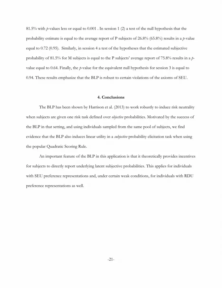
4. Conclusions

The BLP has been shown by Harrison et al. (2013) to work robustly to induce risk neutrality

when subjects are given one risk task defined over objective probabilities. Motivated by the success of

the BLP in that setting, and using individuals sampled from the same pool of subjects, we find

evidence that the BLP also induces linear utility in a subjective probability elicitation task when using

the popular Quadratic Scoring Rule.

An important feature of the BLP in this application is that it theoretically provides incentives

for subjects to directly report underlying latent subjective probabilities. This applies for individuals

with SEU preference representations and, under certain weak conditions, for individuals with RDU

preference representations as well.

-21-

Figure 1: Binary Scoring Rule Using the Binary Lottery Procedure

-22-

Table 1: Experimental Design

Treatment M Treatment P Total

Session 1 17 18 35

Session 2 16 17 33

Session 3 17 16 33

Session 4 18 19 37

Total 68 70 138

Figure 2: Subject Display for Treatment M

-23-

Figure 3: Subject Display for Treatment P

Figure 4: Frequency of Reports by Session

-24-

Figure 5: Estimated Densities of Reports by Session

-25-

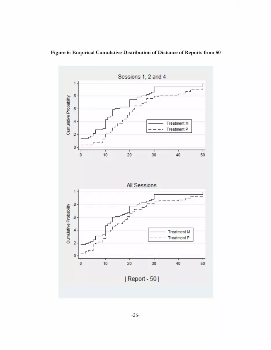
Figure 6: Empirical Cumulative Distribution of Distance of Reports from 50

-26-

Figure 7: Empirical Cumulative Distribution of Distance Pooling Data From All Sessions

-27-

References

Allen, F., 1987. Discovering personal probabilities when utility functions are unknown. ManagementScience 33, 452-454.

Andersen, S., Fountain, J., Harrison, G. W., Rutström, E. E., 2014. Estimating subjectiveprobabilities. Journal of Risk and Uncertainty, forthcoming.

Berg, J. E., Daley, L. A., Dickhaut, J. W., O’Brien, J. R., 1986. Controlling preferences for lotterieson units of experimental exchange. Quarterly Journal of Economics 101, 281-306.

Cox, J. C., Oaxaca, R. L., 1995. Inducing risk-neutral preferences: Further analysis of the data.Journal of Risk and Uncertainty 11, 65-79.

Cox, J. C., Sadiraj, V., Schmidt, U., 2011. Paradoxes and mechanisms for choice underrisk. Working Paper 2011-12, Center for the Economic Analysis of Risk, Robinson Collegeof Business, Georgia State University.

Grether, D. M., 1992. Testing Bayes rule and the representativeness heuristic: Some experimentalevidence. Journal of Economic Behavior and Organization 17, 31-57.

Gul, F., 1991. A theory of disappointment aversion. Econometrica 59, 667-686.

Harrison, G. W., Martínez-Correa, J., Swarthout, J. T., 2012. Reduction of compound lotteries withobjective probabilities: Theory and evidence. Working Paper 2012-05, Center for theEconomic Analysis of Risk, Robinson College of Business, Georgia State University.

Harrison, G. W., Martínez-Correa, J., Swarthout, J. T., 2013. Inducing risk neutral preferences withbinary lotteries: A reconsideration. Journal of Economic Behavior and Organization 94, 145-159.

Harrison, G. W., Swarthout, J. T., 2012. Experimental payment protocols and the bipolarbehaviorist. Working Paper 2012-01, Center for the Economic Analysis of Risk, RobinsonCollege of Business, Georgia State University.

Holt, C. A., Laury, S. K., 2002. Risk aversion and incentive effects. American Economic Review 92,1644-1655.

Holt, C. A., Smith, A. M., 2009. An update on Bayesian updating. Journal of Economic Behaviorand Organization 69, 125-134.

Hossain, T., Okui, R., 2013. The binarized scoring rule. Review of Economic Studies 80, 984-1001.

Karni, E., 2009. A mechanism for eliciting probabilities. Econometrica 77, 603-606.

-28-

Köszegi, B., Rabin, M., 2008. Revealed mistakes and revealed preferences. In: Caplin, A., Schotter,A. (Eds.). The Foundations of Positive and Normative Economics: A Handbook. NewYork: Oxford University Press, 193-209.

Machina, M. J., Schmeidler, D., 1992. A More robust definition of subjective probability.Econometrica 60, 745-780.

Machina, M. J., Schmeidler, D., 1995. Bayes without bernoulli: Simple conditions forprobabilistically sophisticated choice. Journal of Economic Theory 67, 106-128.

McKelvey, R. D., Page, T., 1990. Public and private information: An experimental study ofinformation pooling. Econometrica 58, 1321-1339.

Offerman, T., Sonnemans, J., van de Kuilen, G., Wakker, P. P., 2009. A truth-serum for non-bayesians: Correcting proper scoring rules for risk attitudes. Review of Economic Studies 76,1461-1489.

Roth, A. E., Malouf, M. W. K., 1979. Game-theoretic models and the role of information inbargaining. Psychological Review 86, 574-594.

Rutström, E. E., Wilcox, N. T., 2009. Stated beliefs versus inferred beliefs: A methodological inquiryand experimental test. Games and Economic Behavior 67, 616-632.

Savage, L. J., 1954. The Foundations of Statistics. New York: John Wiley and Sons.

Schlag, K. H., van der Weele, J., 2013. Eliciting probabilities, means, medians, variances andcovariances without assuming risk-neutrality. Theoretical Economics Letters 3, 38-42.

Selten, R., Sadrieh, A., Abbink, K., 1999. Money does not induce risk neutral behavior, but binarylotteries do even worse. Theory and Decision 46, 211-249.

Smith, C. A.B., 1961. Consistency in statistical inference and decision. Journal of the Royal StatisticalSociety 23, 1-25.

Trautmann, S. T., van de Kuilen, G., 2011. Belief elicitation: A horse race among truth serums.CentER Working Paper 2011-117, Tilburg University.

Tversky, A., Kahneman, D., 1992. Advances in prospect theory: Cummulative representation ofuncertainty. Journal of Risk and Uncertainty 5, 297-323.

Yaari, M. E., 1987. The dual theory of choice under risk. Econometrica 55, 95-115.

-29-