arX

iv:q

uant

-ph/

0609

021v

1 4

Sep

200

6

Quantum probabilities for time-extended

alternatives

Charis Anastopoulos∗

Department of Physics, University of Patras, 26500 Patras, Greece

and

Ntina Savvidou †

Theoretical Physics Group, Imperial College, SW7 2BZ, London, UK

February 1, 2008

Abstract

We study the probability assignment for the outcomes of time-extended

measurements. We construct the class-operator that incorporates the in-

formation about a generic time-smeared quantity. These class-operators

are employed for the construction of Positive-Operator-Valued-Measures

for the time-averaged quantities. The scheme highlights the distinction

between velocity and momentum in quantum theory. Propositions about

velocity and momentum are represented by different class-operators, hence

they define different probability measures. We provide some examples,

we study the classical limit and we construct probabilities for generalized

time-extended phase space variables.

1 Introduction

In this article we study the probability assignment for quantum measurementsof observables that take place in finite time. Usually measurements are treatedas instantaneous. One assumes that the duration of interaction between themeasured system and the macroscopic measuring device is much smaller thanany macroscopic time scale characterising the behaviour of the measurement de-vice. Although this is a reasonable assumption, measurements that take placein a macroscopically distinguishable time interval are theoretically conceivable,too. In the latter case one expects that the corresponding probabilities wouldbe substantially different from the ones predicted by the instantaneous approx-imation. Moreover, the consideration of the duration of the measurement as

∗anastop@physics.upatras.gr†ntina@imperial.ac.uk

1

a determining parameter allows one to consider observables whose definitionexplicitly involves a finite time interval. Such observables may not have a nat-ural counterpart when restricted to single-time alternatives. In what follows,we also study physical quantities whose definition involves time-derivatives ofsingle-time observables.

There are different procedures we can follow for the study of finite-timemeasurements. For example, one may employ standard models of quantummeasurement and refrain from taking the limit of almost instantaneous interac-tion between the measuring system and the apparatus [1]. However, there is anobvious drawback. For example, a measurement of momentum can be imple-mented by different models for the measuring device. They all give essentiallya probability that is expressed in terms of momentum spectral projectors (moregenerally positive operators). However, if one considers a measurement of finiteduration, it is not obvious to identify the physical quantity of the measuredsystem to which the resulting probability measure corresponds.

This problem is especially pronounced when one considers measurements ofrelatively large duration. For the reason above, we choose a different startingpoint: we identify time-extended classical quantities and the we construct cor-responding operators that act on the Hilbert space of the measured system.A special case of such observables are quantities that are smeared in time. Ifan operator A has (generalised) eigenvalues a, then we identify a probability

density for its time-smeared values 〈a〉f =∫ T

0dt atf(t). Here f(t) is a positive

function defined on the interval [0, T ]. The special case f(t) = 1T corresponds

to the usual notion of time-averaging.Having identified the operators that represent the time-extended quantities,

it is easy to construct the corresponding probability measure for such observablesusing for example, simple models for quantum measurement.

Our analysis is facilitated by a comparison with the decoherent histories ap-proach to quantum mechanics [2, 3, 4, 5]. The identification of operators thatcorrespond to time-extended observables is structurally similar to the descrip-tion of temporally extended alternatives in the decoherent histories approach[6, 7, 8, 9, 10, 11, 12]. The physical context is different, in the sense that the de-coherent histories scheme attempts the description of individual closed systems,while the study of measurements we undertake here involves—by necessity—theconsideration of open systems. However, the mathematical descriptions are veryclosely related.

A history is defined as a sequence of propositions about the physical systemat successive moments of time. A proposition in quantum mechanics is repre-sented by a projection operator; hence, a general n-time history α correspondsto a string of projectors {Pt1 , Pt2 , . . . , Ptn

}. To determine the probabilities as-sociated to these histories we define the class operator Cα,

Cα = U †(t1)Pt1 U(t1) . . . U†(tn)Ptn

U(tn), (1)

2

where U(t) = e−iHt is the evolution operator for the system. For a pair ofhistories α and α′, we define the decoherence functional

d(α, α′) = Tr(

C†αρ0Cα′

)

. (2)

A key feature of the decoherent histories scheme is that probabilities can beassigned to an exclusive and exhaustive set of histories only if the decoherencecondition

d(α, α′) = 0, α 6= α′ (3)

holds. In this case one may define a probability measure on this space of histories

p(α) = Tr(

C†αρCα

)

. (4)

One of the most important features of the decoherent histories approach is itsrich logical structure: logical operations between histories can be representedin terms of algebraic relations between the operators that represent a history.This logical structure is clearly manifested in the History Projection Operator(HPO) formulation of decoherent histories [13]. In this paper we will make useof the following property. If {αi} is a collection of mutually exclusive histories,each represented by the class operator Cαi

then the coarse-grained history thatcorresponds to the statement that any one of the histories i has been realisedis represented by the class operator

∑

i Cαi. This property has been employed

by Bosse and Hartle [12], who define class operators corresponding to time-averaged position alternatives using path-integrals. A similar construction in aslightly different context is given by Sokolovski et al [14, 15]—see also Ref. [16].

Our first step is to generalise the results of [12] by constructing such classoperators for the case of a generic self-adjoint operator A that are smeared withan arbitrary function f(t) within a time interval [0, T ]. This we undertake insection 2.

In section 3, we describe a toy model for a time-extended measurement. Itleads to a probability density for the measured observable that is expressed solelyin terms of the class operators Cα. The same result can be obtained withoutthe use of models for the measurement device through a purely mathematicalargument. We identify generic Positive-Operator-Valued Measure (POVM) thatis bilinear with respect to the class operators Cα and compatible with Eq. (4).

The result above implies that Cα can be employed in two different roles:first, as ingredients of the decoherence functional in the decoherent historiesapproach and second, as building block of a POVM in an operational approachto quantum theory. The same mathematical object plays two different roles: in[12] class operators corresponding to time-average observables are constructedfor use within the decoherent histories approach, while the same objects areused in [15] for the determination of probabilities of time-extended positionmeasurements.

3

The approach we follow allows the definition of more general observables.Within the context of the HPO approach, velocity and momentum are rep-resented by different (non-commuting) operators: they are in principle distin-guishable concepts [9].

In section 4, we show that indeed one may assign class operators to alter-natives corresponding to values of velocity that are distinct from those corre-sponding to values of momentum. These operators coincide at the limit of largecoarse-graining (which often coincides with the classical limit). In effect, twoquantities that coincide in classical physics are represented by different objectsquantum mechanically. It is quite interesting that the POVMs correspondingto velocity are substantially different from those corresponding to momentum.At the formal level, it seems that quantum theory allows the existence of instru-ments which are able to distinguish between the velocity and momentum of aquantum particle. A priori, this is not surprising: in single-time measurements,velocity cannot be defined as an independent variable. For extended-in-timemeasurements, it is not inconceivable that one type of detector responds to therate of change of the position variable and another to the particle’s momen-tum. Whether this result is a mere mathematical curiosity, or whether onecan design experiments that will demonstrate this difference completely will beaddressed in a future publication. In section 4 we also study more general time-extended measurements, namely ones that correspond to time-extended phasespace properties of the quantum system.

2 Operators representing time-averaged quanti-

ties

2.1 The general form of the class operators

We construct the class operators that correspond to the proposition “the valueof the observable A, smeared with a function f(t) within a time interval [0, T ],takes values in the subset U of the real line R.”

We denote by at a possible value of the observable A at time t. Then at the

continuous-time limit the time-smeared value Af of A reads Af :=∫ T

0 atf(t)dt.

Note that for the special choice f(t) = 1T χ[0,T ](t), where χ[0,T ] is the characteris-

tic function of the interval [0, T ], we obtain the usual notion of the time-averagedvalue of a physical quantity.

There are two benefits from the introduction of a general function f(t). First,it can be chosen to be a continuous function of t, thus allowing the considerationof more general ‘observables’; for example observables that involve the timederivatives of at. Second, when we consider measurements, the form of f(t)may be determined by the operations we effect on the quantum system. Forexample, f(t) may correspond to the shape of an electromagnetic pulse actingupon a charged particle during measurement.

4

To this end, we construct the relevant class operators in a discretised form.We partition the interval [0, T ] into n equidistant time-steps t1, t2, . . . , tn. The

integral∫ T

0dtf(t)at is obtained as the continuous limit of δt

∑

i f(ti)ati=

Tn

∑

i f(ti)ati.

For simplicity of exposition we assume that the operator A has discretespectrum, with eigenvectors |ai〉 and corresponding eigenvalues ai

1. We writePai

= |ai〉〈ai|. By virtue of Eq. (1) we construct the class operator

Cα = eiHT/n|a1〉〈a1|eiHT/n|a2〉〈a2| . . . 〈an−1|eiHT/n|an〉〈an| (5)

that represents the history α = (a1, . . . , an).The proposition “the time-averaged value of A lies in a subset U of the real

line” can be expressed by summing over all operators of the form of Eq. (5),for which T

n

∑

i f(ti)ai ∈ U ,

CU =∑

a1,a2,...,an

χU

(

T

n

∑

i

f(ti)ai

)

× eiHT/n|a1〉〈a1|eiHT/n|a2〉〈a2| . . . 〈an−1|eiHT/n|an〉〈an|. (6)

If we partition the real axis of values of the time-averaged quantity Af intomutually exclusive and exhaustive subsets Ui, the corresponding alternatives forthe value of Af will also be mutually exclusive and exhaustive.

Next, we insert the Fourier transform χU of χU defined by

χU (x) :=

∫

dk

2πeikxχU (k) (7)

into Eq. (6). We thus obtain

CU =

∫

dk

2πχU (k)e−iHT/n

(

∑

a1

e−ikTf(t1)a1/n|a1〉〈a1|)

eiHT/n . . .

×eiHT/n

(

∑

an

e−ikTf(tn)an/n|an〉〈an|)

. (8)

By virtue of the spectral theorem we have∑

ai

eikTf(ti)ai/n|ai〉〈ai| = eikf(ti)A/n. (9)

Hence,

CU =

∫

dk

2πχU (k)

n∏

i=1

[eiHT/neikf(ti)AT/n]. (10)

1The generalization of our results for continuous spectrum is straightforward.

5

From Eq. (10) we obtain

CU =

∫

U

da C(a), (11)

where

C(a) :=

∫

dk

2πe−ikaUf (T, k), (12)

and where

Uf(T, k) := limn→∞

n∏

i=1

[eiHT/ne−ikf(ti)AT/n]. (13)

The operator Uf is the generator of an one-parameter family of transformations

−i ∂∂sUf (s, k) = [H + kf(s)A]Uf(s, k). (14)

This implies that

Uf (T, k) = T ei∫

T

0dt(H+kf(t)A)

, (15)

where T signifies the time-ordered expansion for the exponential. The construc-tion of CU then is mathematically identical to the determination of a propagatorin presence of a time-dependent external force proportional to A.

For f(t) = 1T χ[0,T ](t) we obtain

CU =

∫

dk

2πχU (k)eiHT+ikA, (16)

that has been constructed through path-integrals for specific choices of the op-erator A in [14, 15, 12].

If f(t) has support in the interval [t, t′] ⊂ [0, T ] then

CU = e−iHt

∫

U

da

(∫

dk

2πe−ikaT ei

∫

t′

tds(H+kf(s)A)

)

eiH(T−t′). (17)

We note that outside the interval [t, t′] only the Hamiltonian evolution con-tributes to CU outside the interval [t, t′].

It will be convenient to represent the proposition about the time-averagedvalue of A by the operator

D(a) := e−iHT C(a), (18)

or else

D(a) =

∫

dk

2πe−ika T eik

∫

T

0dtf(t)A(t)

, (19)

6

where A(t) is the Heisenberg-picture operator eiHtAe−iHt.If [H, A] = 0, then

Uf (T, k) = eiA∫

T

0dtf(t)

. (20)

Hence,

DU :=

∫

U

daD(a) = χU [A

∫ T

0

dtf(t)]. (21)

When we use f(t) to represent time-smearing, it is convenient to require that∫ T

0 dtf(t)) = 1 in order to avoid any rescaling in the values of the observable.

Then DU = χU (A). We conclude therefore that the operator representing time-averaged value of A coincides with the one representing a single-time value ofA.

The limit of large coarse-graining. If we integrate D(a) over a relativelylarge sample set U the integral over dk is dominated by small values of k. Tosee this, we approximate the integration over a subset of the real line of width∆ centered around a = a0, by an integral with a smeared characteristic functionexp[−(a− a0)

2/2∆2]. This leads to

DU =√

2π∆

∫

dk

2πe−∆2k2/2 T ei

∫

T

0dtf(t)A(t)

(22)

that is dominated by values of k ∼ ∆−1 .The term kf(t) in the time-ordered exponential of Eq. (19) is structurally

similar to a coupling constant. Hence, for sufficiently large values of ∆ we write

T ei∫

T

0dtf(t)A(t) ≃ e

i∫

T

0dtf(t)A(t)

, (23)

i.e., the zero-th loop order contribution to the time-ordered exponential domi-nates. We therefore conclude that

DU ≃ χU

[

∫ T

0

dtf(t)A(t)

]

. (24)

DU is almost equal to a spectral element of the time-averaged Heisenberg-picture

operator∫ T

0dtf(t)A(t). This generalises the result of [12], which was obtained

for configuration space variables at the limit h→ 0.We estimate the leading order correction to the approximation involved in

Eq. (24). The immediately larger contribution to the time-ordered exponentialof Eq. (19) is

k2

2

∫ T

0

ds

∫ s

0

ds′ f(s)f(s′) [A(s), A(s′)]. (25)

7

The contribution of this term must be much smaller than the first term in theexpansion of the time-ordered exponential’s, namely k

∫ T

0dsf(s)A(s). We write

the expectation values of these operators on a vector |ψ〉 in order to obtain thefollowing condition

|∫ T

0

ds

∫ s

0

ds′f(s)f(s′)〈ψ|[A(s), A(s′)]|ψ〉| << ∆ |∫ T

0

ds〈ψ|A(s)|ψ〉|. (26)

The above condition is satisfied rather trivially for bounded operators if||A|| << ∆. In that case, the operator CU captures little, if anything, from thepossible values of A. In the generic case however, Eq. (26) is to be interpretedas a condition on the state |ψ〉. Eq. (24) provides a good approximation if thetwo-time correlation functions of the system are relatively small.

Furthermore, if the function f(t) corresponds to weighted averaging, i.e., if

f(t) ≥ 0, and if f does not have any sharp peaks, then the condition∫ T

0 dtf(t) =

1 implies that the values of f(t) are of the order 1T .

We denote by τ the correlation time of A(s), i.e. the values of |s − s′| forwhich |〈ψ|[A(s), A(s′)]|ψ〉| is appreciably larger than zero. Then at the limit

T >> τ the left-hand side of Eq. (26) is of the order O(

τ2

T 2

)

. Hence, for

sufficiently large values of T one expects that Eq. (24) will be satisfied with afair degree of accuracy.

The argument above does not hold if f is allowed to take on negative values,which is the case for the velocity samplings that we consider in section 4.

2.2 Examples

We study some interesting examples of class operators corresponding to time-smeared quantities. In particular, we consider the time-smeared position for aparticle.and a simple system that is described by a finite-dimensional Hilbertspace.

2.2.1 Two-level system

In a two-level system described by the Hamiltonian H = ωσz, we considertime-averaged samplings of the values of the operator A = σx. We compute

U(k, T ) = cos√

k2 + ω2T 2 1 + isin

√k2 + ω2T 2

√k2 + ω2T 2

(kσx + ωT σz). (27)

Then the class operator C(a) is

C(a) =ωT

2√

1 − a2J1(ωT

√

1 − a2) 1 +aωT

2√

1 − a2J1(ωT

√

1 − a2)σx

+iωT

2J0(ωT

√

1 − a2)σz , (28)

8

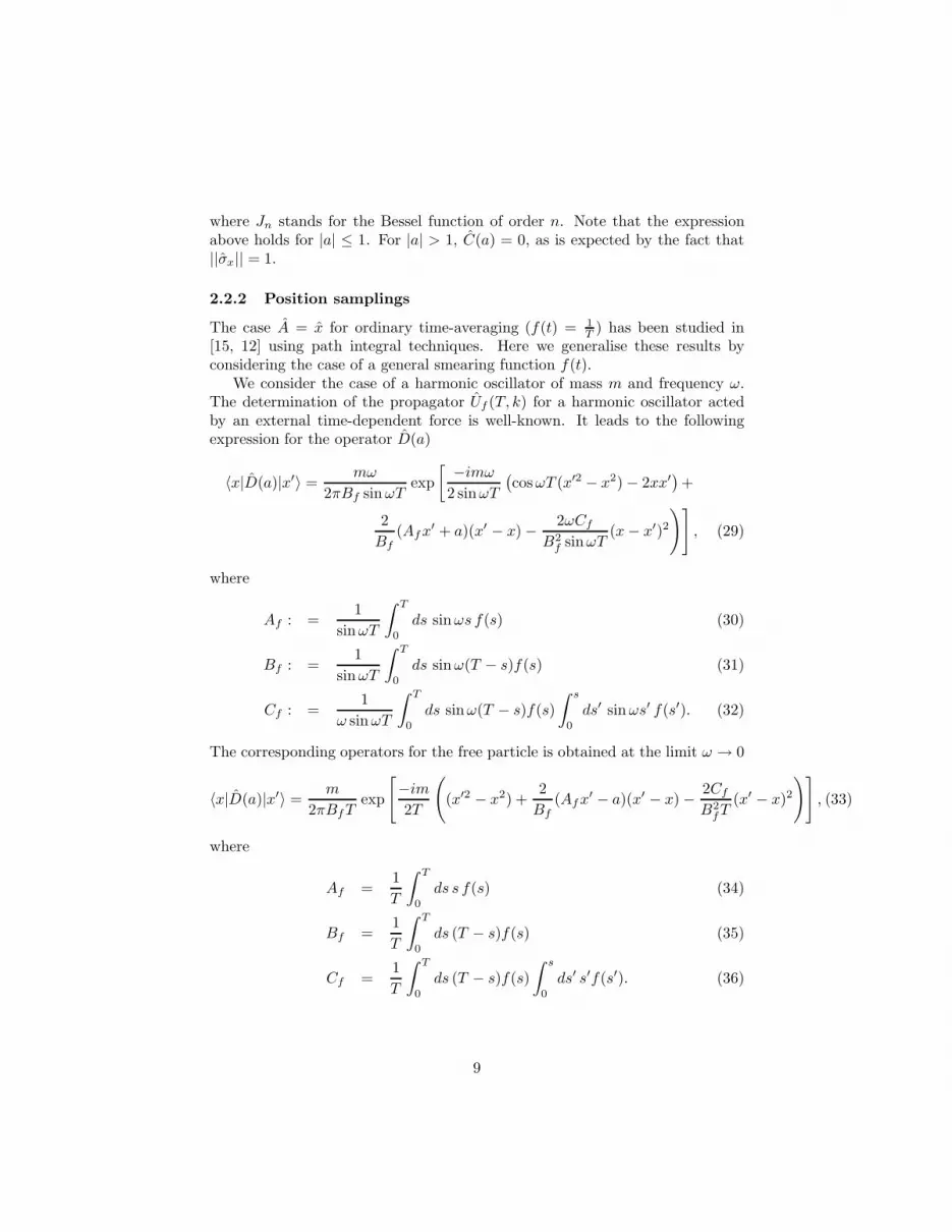
where Jn stands for the Bessel function of order n. Note that the expressionabove holds for |a| ≤ 1. For |a| > 1, C(a) = 0, as is expected by the fact that||σx|| = 1.

2.2.2 Position samplings

The case A = x for ordinary time-averaging (f(t) = 1T ) has been studied in

[15, 12] using path integral techniques. Here we generalise these results byconsidering the case of a general smearing function f(t).

We consider the case of a harmonic oscillator of mass m and frequency ω.The determination of the propagator Uf (T, k) for a harmonic oscillator actedby an external time-dependent force is well-known. It leads to the followingexpression for the operator D(a)

〈x|D(a)|x′〉 =mω

2πBf sinωTexp

[ −imω2 sinωT

(

cosωT (x′2 − x2) − 2xx′)

+

2

Bf(Afx

′ + a)(x′ − x) − 2ωCf

B2f sinωT

(x− x′)2

)]

, (29)

where

Af : =1

sinωT

∫ T

0

ds sinωs f(s) (30)

Bf : =1

sinωT

∫ T

0

ds sinω(T − s)f(s) (31)

Cf : =1

ω sinωT

∫ T

0

ds sinω(T − s)f(s)

∫ s

0

ds′ sinωs′ f(s′). (32)

The corresponding operators for the free particle is obtained at the limit ω → 0

〈x|D(a)|x′〉 =m

2πBfTexp

[

−im2T

(

(x′2 − x2) +2

Bf(Afx

′ − a)(x′ − x) − 2Cf

B2fT

(x′ − x)2

)]

, (33)

where

Af =1

T

∫ T

0

ds s f(s) (34)

Bf =1

T

∫ T

0

ds (T − s)f(s) (35)

Cf =1

T

∫ T

0

ds (T − s)f(s)

∫ s

0

ds′ s′f(s′). (36)

9

3 Probability assignment

3.1 The decoherence functional

For a pair of histories (U,U ′) that correspond to different samplings of thetime-smeared values of A the decohrence functional d(U,U ′) is

d(U,U ′) = Tr(

D†Ue

−iHT ρ0eiHT DU ′

)

. (37)

From the expression above, we can read the probabilities that are associatedto any set of alternatives that satisfies the decoherence condition. In section 2,we established that in the limit of large coarse-graining, or for very large valuesof time T , the operators DU approximate projection operators. Hence, if wepartition the real line of values of Af into sufficiently large exclusive sets Ui thedecoherence condition will be satisfied. A probability measure will be thereforedefined as

p(Ui) = Tr

[

χUi

(

∫ T

0

dtf(t)A(t)

)

e−iHT ρ0eiHT

]

. (38)

This is the same as in the case of a single-time measurement of the observable∫ T

0dtf(t)A(t) taking place at time t = T . For further discussion, see [12].

3.2 Probabilities for measurement outcomes

Next, we show that the class operators C(a) can be employed in order to define aPOVM for a measurement with finite duration. For this purpose, we consider asimple measurement scheme. We assume that the system interacts with a mea-surement device characterised by a continuous pointer basis |x〉. For simplicity,we assume that the self-dynamics of the measurement device is negligible. Theinteraction between the measured system and the apparatus is described by aHamiltonian of the form

Hint = f(t)A⊗ K, (39)

where K is the ‘conjugate momentum’ of the pointer variable x

K =

∫

dk k |k〉〈k|, (40)

where 〈x|k〉 = 1√2πe−ikx. The initial state of the apparatus (at t = 0) is

assumed to be |Ψ0〉 and the initial state of the system corresponds to a densitymatrix ρ0.

With the above assumptions, the reduced density matrix of the apparatusat time T is

ρapp(T ) =

∫

dk

∫

dk′ Tr(

U †f (T, k)ρ0Uf (T, k′)

)

〈k|Ψ0〉〈Ψ0|k′〉 |k〉〈k′|, (41)

10

where Uf (T, k) is given by Eq. (15). Then, the probability distribution over thepointer variable x (after reduction) is

〈x|ρapp(T )|x〉 =

∫

dkdk′

2πe−i(k−k′)x〈k|Ψ0〉〈Ψ0|k′〉 Tr

(

U †f (T, k)ρ0Uf(T, k′)

)

. (42)

The probability that the pointer variable takes values within a set U is

p(U) = tr(

e−iHT ρ0eiHT ΠU

)

, (43)

where

ΠU =

∫

U

dx D(w∗x)D†(wx) :=

∫

U

dx Πx, (44)

where wx(a) := 〈x− a|Ψ0〉 and where we employed the notation

D(wx) =

∫

dawx(a)D(a), (45)

The operators ΠU define a POVM for the time-extended measurement of A:they are positive by construction, they satisfy the property ΠU1∪U2

= ΠU1+ΠU2

,for U1 ∩ U2 = ∅ and they are normalised to unity

ΠR =

∫

R

dx Πx = 1. (46)

Note that the smearing of the class-operators is due to the spread of thewave function of the pointer variable.

In what follows we employ for convenience a Gaussian function

w(a) =1

(2πδ2)1/4e−

a2

4δ2 . (47)

In the free-particle case, the class operators in Eq. (33) lead to the followingPOVM

〈y|Πx|y′〉 =m√

2πAfTexp

[

−(

m2δ2

2A2fT

2+A2

f

8δ2(1 − 2Cf

A2fT

)2

)

(y − y′)2 +im

AfTx(y′ − y)

]

. (48)

In Eq. (48), we chose an even time-averaging function, i.e. f(s) = f(T − s),in which case Af = Bf .

The POVM in Eq. (44) may also be constructed without reference to a spe-cific model for the measurement device. In particular, we partition the space ofvalues for Af into sets of width δ and employ the expression Eq. (4) for the ensu-ing probabilities. It is easy to show that these probabilities are reproduced—up

11

to terms of order O(δ)—by a POVM of the form Eq. (44), with the smearingfunction w of Eq. (47) 2.

If we restrict our considerations to the above measurement model, then thereis no way we can interpret the POVM of Eq. (44) as corresponding to valuesof Af , This interpretation is possible by the explicit construction and by the

identification (see Sec. 2) of the class operators C(a) as the only mathematicalobjects that correspond to such time-averaged alternatives.

4 More general samplings

4.1 Velocity Vs momentum

Within the context of the History Projection Operator scheme, Savvidou showedthat histories of momentum differ in general from histories of velocity, in thesense that they are represented by different mathematical objects [9]. Thecorresponding probabilities are also expected to be different. In single-timequantum theory the notion of velocity (that involves differentiation with respectto time) cannot be distinguished from the notion of momentum. However,when we deal with histories, time differentiation is defined independently ofthe evolution laws. One may therefore consider alternatives corresponding todifferent values of velocity.

In particular, if xf =∫ T

0 dtxtf(t) denotes the time-smeared value of theposition variable, we define the time-smeared value of the corresponding velocityvariable as

xf := −xf , (49)

provided that the function f satisfies f(0) = f(T ) = 0.Notice here that when we measure the time-averaged value of an observable

within a time-interval [0, T ], we employ positive functions f(t) that are ∩-shaped

and that they satisfy∫ T

0dtf(t) = 1. Such functions correspond to the intuitive

notions of averaging the value of a quantity with a specific weight.However, to determine the time-average velocity—weighted by a positive

and normalised function f—one has to smear the corresponding position vari-able with the function f(t) that in the general case is neither positive nor nor-malised. Therefore the form of the smearing function determines the physical

interpretation of the observable we consider [18].Next, we compare the class operators corresponding to the average of velocity

and of momentum, with a common weight f . We denote the velocity classoperator as

Dx(a) =

∫

dk

2πe−ikaT ei

∫

T

0dt f(t)x(t)

, (50)

2The proof follows closely an analogous one in [17]).

12

and the momentum class operators as

Dp(a) =

∫

dk

2πe−ikaT ei

∫

T

0dt f(t)p(t)

. (51)

At the limit of large coarse-graining, the operator DxU :=

∫

U da Dx(a) is

approximately equal to

DxU = χU (

∫ T

0

dtf(t)x(t)) = χU (1

m

∫ T

0

dt f(t)p(t)), (52)

i.e., the class-operator for time-averaged momentum coincides with that fortime-averaged velocity. This result reproduces the classical notion that p = mx.However, the limit of large coarse-graining may be completely trivial if thetemporal correlations of position are large.

For the case of a free particle, with the convenient choice f(t) = πT sin πt

T ,we obtain

DpU =

∫

U

dp |p〉〈p|, (53)

DxU =

∫

U

da

(

√

4imT

π3

∫

dp ei 4mT

π2(a−p/m)2 |p〉〈p|

)

. (54)

It is clear that the alternatives of time-averaged momentum are distinct fromthose of time-averaged velocity. Still, at the limit T → ∞, Dp

U = mDxU .

The POVM corresponding to Eq. (54) is

Πx(v) =1

√

2πσ2(T )

∫

dp exp

[

− 1

2σ2v(T )

(v − p/m)2]

|p〉〈p|, (55)

where σ2v(T ) = δ2 + π4

28m2T 2δ2 .The POVM of Eq. (55) commutes with the momentum operator. One could

therefore claim that it corresponds to an unsharp measurement of momentum.However, the commutativity of this POVM with momentum follows only fromthe special symmetry of the Hamiltonian for a free-particle, it does not hold ingeneral. Moreover, at the limit of small T , the distribution corresponding to Eq.(55) has a very large mean deviation. Hence, even for a wave-packet narrowlyconcentrated in momentum, the spread in measured values is large. Note that atthe limit T → 0, the deviation σ2

v(T ) → ∞ and the POVM (55) tends weakly tozero. For T >> (mδ2)−1, then σ2

v(T ) ≃ δ2 and the velocity POVM is identicalto one obtained by an instantaneous momentum measurement.

The results of section 3.2 suggest the different measurement schemes thatare needed for the distinction of velocity and momentum. For a momentummeasurement the interaction Hamiltonian should be of the form

Hpint = f(t) p ⊗ K, (56)

13

where f(t) is a ∩-shaped positive-valued function. For a velocity measurementthe interaction Hamiltonian is

H xint = −f(t) x⊗ K. (57)

The two Hamiltonians differ not only on the coupling but also on the shapeof the corresponding smearing functions: f(t) takes both positive and negative

values and by definition it satisfies∫ T

0f(t) = 0. The description above suggests

that momentum measurements can be obtained by coupling a charged particleto a magnetic field pulse, while velocity measurements can be obtained by acoupling to an electric field pulse of a different shape. The possibility of design-ing realistic experiments that could distinguish between the momentum and thevelocity content of a quantum state will be discussed elsewhere.

4.2 Lagrangian action

One may also consider samplings corresponding to the values of the Lagrangian

action of the system∫ T

0dtL(x, x), where L is the Lagrangian. In this case

the results can be easily expressed in terms of Feynman path integrals: it isstraightforward to demonstrate—see Ref. [14]—that these coincide with sam-plings of the Hamiltonian, and that the corresponding POVM is that of energymeasurements.

4.3 Phase space properties

It is possible to construct class-operators (and corresponding POVMs) for moregeneral alternatives that involve phase-space variables. To see this, we considera set of coherent states |z〉 on the Hilbert space, where z denotes points of thecorresponding classical phase space. The finest-grained histories correspondingto an n-time coherent state path z0, t0, z1, t1, . . . zn, tn, with ti − ti−1 = δt arerepresented by the class operator

Cz0,t0;z1,t1;...;zn,tn= |z0〉〈z0|eiHδt|z1〉〈z1|eiHδt|z2〉 · · · 〈zn−1|eiHδt|zn〉〈zn|. (58)

We use the standard Gaussian coherent states, which are defined through aninner product

〈z|z′〉 = e−|z|2

2− |z′|2

2+z∗z′

. (59)

Then, at the limit of small δt

Cz1,t1;z2,t2;...;zn,tn= |z0〉〈zn| exp

(

|zn|22

− |z0|22

−n∑

i=1

z∗i (zi − zi−1) + iδt h(z∗i , zi−1)

)

, (60)

where h(z∗, z) = 〈z|H|z〉. Following the same steps as in section 2.1 we con-struct the class operator corresponding to different values of an observable

14

A(z0, z1, . . . , zn). If the observable is ultra-local, i.e., if it can be written inthe form

∑

i f(ti)a(zi), then the results reduce to those of section 2.1 for thetime-smeared alternatives of an operator.

However, the function in question may involve time derivatives of phase spacevariables (at the continuous limit), in which case it will be rather different fromthe ones we considered previously. For a generic function F (zi) we obtain thefollowing class operator that corresponds to the value F = a

〈z0|C(a)|zf 〉 =

∫

dk

2πe−ika lim

n→∞

∫

[dz1] . . . [dzn−1]

× exp

[

|zn|22

− |z0|22

+∑

i

zi(z∗i − z∗i−1) + iδt h(z∗i , zi−1) − ikF [zi]

]

. (61)

The integrations over [dzi] defines a coherent-state path-integral at the continu-ous limit. However, if F [zi] is not an ultra-local function, the path integral does

not correspond to a unitary operator of the form T e∫

T

0dtKt , for some family of

self adjoint operators Kt. In this sense, the consideration of phase space pathsprovides alternatives that do not reduce to those studied in Section 2. Notehowever, that these alternatives cannot be defined in terms of projection oper-ators; nonetheless the corresponding class operators can be employed to definea POVM using Eq. (44).

The simplest non-trivial example of a non-ultralocal function is the Liouvilleterm of the phase space action ( for its physical interpretation in the historiestheory see [9])

V := i

∫ T

0

dtz∗z. (62)

It is convenient to employ the discretised expression V = i∑n

i=1 zi(z∗i − z∗i−1).

Its substitution in Eq. (61) effects a multiplication of the Liouville term in theexponential by a factor of 1 + k.

For an harmonic oscillator Hamiltonian h(z∗, z) = ωz∗z, and the path inte-

gral can be explicitly computed yielding the unitary operator ei

1+kHT . Hence,

C(a) =

∫

dk

2πe−ikae

i

1+kHT = sa(H), (63)

where sa(x) :=∫

dk2π e

−ika+i x

1+k . The class-operator C(a) corresponding tothe values of the function V is then a function of the Hamiltonian.

5 Conclusions

We studied the probability assignment for time-extended measurements. Weconstructed of the class operators C(a), which correspond to time-extended

15

alternatives for a quantum system. We showed that these operators can beemployed to construct POVMs describing the probabilities for time-averagedvalues of a physical quantity. In light of these results, quantum mechanicshas room for measurement schemes that distinguish between momentum andvelocity. Finally, we demonstrated that a large class of time-extended phasespace observables may be explicitly constructed.

Acknowledgements

C.A. was funded by a Pythagoras II grant (EPEAEK). N.S. acknowledges sup-port from the EP/C517687 EPSRC grant.

References

[1] A. Peres and W. K. Wooters, Phys. Rev. D32, 1968 (1985); A. Peres, Phys.Rev. A61, 022116 (2000).

[2] R. Griffiths, J. Stat. Phys. 36, 219 (1984).

[3] R. Omnes, J. Stat. Phys. 53, 893 (1988); The Interpretation of Quantum

Mechanics, (Princeton University Press, Princeton, 1994); Rev. Mod. Phys.64, 339 (1992).

[4] M. Gell-Mann and J. B. Hartle, in Complexity, Entropy and the Physics of

Information, edited by W. Zurek, (Addison Wesley, Reading, 1990); Phys.Rev. D 47, 3345 (1993).

[5] J. B. Hartle, Spacetime Quantum Mechanics and the Quantum Mechanics

of Spacetime, in Proceedings on the 1992 Les Houches School, Gravitationand Quantisation, 1993.

[6] J. B. Hartle, Phys. Rev. D44, 3173 (1991).

[7] N. Yamada and S. Tagaki, Prog. Theor. Phys. 85, 985 (1991); 86, 599 (1991);87, 77 (1992).

[8] C. J. Isham and N. Linden, J. Math. Phys. 36, 5392 (1995); C. J. Isham, N.Linden, K. Savvidou and S. Schreckenberg, J. Math. Phys. 39, 1818 (1998).

[9] K. Savvidou, J. Math. Phys. 40, 5657 (1999).

[10] R. J. Micanek and J. B. Hartle, Phys. Rev. A 54, 37953800 (1996).

[11] J. J. Halliwell, Decoherent Histories for Space-Time Domains, LectureNotes in Physics (Springer Berlin / Heidelberg, 2002).

[12] A. W. Bosse and J. B. Hartle, Phys. Rev. A 72, 022105 (2005).

16

[13] C. J. Isham, J. Math. Phys. 35, 2157 (1994); C. J. Isham and N. Linden,J. Math. Phys. 35, 5452 (1994).

[14] D. Sokolovski, Phys. Rev. A 57, R1469 (1998); Phys. Rev. A 59, 1003(1999).

[15] Y. Liu and D. Sokolovski, Phys. Rev. A 63, 014102 (2001).

[16] C. Caves, Phys. Rev. D33, 1643 (1986).

[17] C. Anastopoulos, quant-ph/0509019.

[18] N. Savvidou, Braz. J. Phys. 35, 307 (2005).

17