EMIC Intercomparison Project (EMIP–CO2): comparative analysis of EMIC simulations of climate, and of equilibrium and transient responses to atmospheric CO2 doubling

ORIGINAL ARTICLE

V. Petoukhov Æ M. Claussen Æ A. Berger Æ M. Crucifix

M. Eby Æ A. V. Eliseev Æ T. Fichefet Æ A. Ganopolski

H. Goosse Æ I. Kamenkovich Æ I. I. Mokhov

M. Montoya Æ L. A. Mysak Æ A. Sokolov Æ P. StoneZ. Wang Æ A. J. Weaver

EMIC Intercomparison Project (EMIP–CO2): comparative analysisof EMIC simulations of climate, and of equilibrium and transientresponses to atmospheric CO2 doubling

Received: 4 February 2005 / Accepted: 2 May 2005 / Published online: 23 July 2005� Springer-Verlag 2005

Abstract An intercomparison of eight EMICs (Earthsystem Models of Intermediate Complexity) is carriedout to investigate the variation and scatter in the

results of simulating (1) the climate characteristics atthe prescribed 280 ppm atmosphere CO2 concentration,and (2) the equilibrium and transient responses to CO2

doubling in the atmosphere. The results of the first partof this intercomparison suggest that EMICs are inreasonable agreement with the present-day observa-tional data. The dispersion of the EMIC results by andlarge falls within the range of results of General Cir-culation Models (GCMs), which took part in theAtmospheric Model Intercomparison Project (AMIP)and Coupled Model Intercomparison Project, phase 1(CMIP1). Probable reasons for the observed discrep-ancies among the EMIC simulations of climate char-acteristics are analysed. A scenario with gradualincrease in CO2 concentration in the atmosphere (1%per year compounded) during the first 70 years fol-lowed by a stabilisation at the 560 ppm level during aperiod longer than 1,500 years is chosen for the secondpart of this intercomparison. It appears that the EMICresults for the equilibrium and transient responses toCO2 doubling are within the range of the correspond-ing results of GCMs, which participated in the atmo-sphere-slab ocean model intercomparison project andCoupled Model Intercomparison Project, phase 2(CMIP2). In particular EMICs show similar tempera-ture and precipitation changes with comparable mag-nitudes and scatter across the models as found in theGCMs. The largest scatter in the simulated response ofprecipitation to CO2 change occurs in the subtropics.Significant differences also appear in the magnitude ofsea ice cover reduction. Each of the EMICs partici-pating in the intercomparison exhibits a reduction ofthe strength of the thermohaline circulation in theNorth Atlantic under CO2 doubling, with the maxi-mum decrease occurring between 100 and 300 yearsafter the beginning of the transient experiment. Afterthis transient reduction, whose minimum notably varies

V. Petoukhov (&) Æ M. Claussen Æ A. GanopolskiPotsdam Institute for Climate Impact Research,GermanyE-mail: [email protected]: +49-331-2882570

A. Berger Æ M. Crucifix Æ T. Fichefet Æ H. GoosseInstitut d‘Astronomie et de Geophysique Georges Lemaıtre,Universite Catholique de Louvain, Belgium

Present address: M. CrucifixHadley Centre for Climate Prediction and Research,Met Office, Exeter, Devon, UK

M. Eby Æ A. J. WeaverSchool of Earth and Ocean Sciences,University of Victoria, Canada

A. V. Eliseev Æ I. I. MokhovA.M.Obukhov Institute of Atmospheric Physics,Russian Academy of Sciences, Russia

I. KamenkovichDepartment of Atmospheric Sciences,Joint Institute for the Study of the Atmosphere and the Oceans,University of Washington, Seattle, USA

M. MontoyaDpto. Astrofisica y Ciencias de la Atmosfera,Facultad de Ciencias Fisicas,Universidad Complutense de Madrid, Spain

L. A. Mysak Æ Z. WangDepartment of Atmospheric and Oceanic Sciences,McGill University, Montreal, Canada

A. SokolovJoint Program on the Science and Policy of Global Change,Massachusetts Institute of Technology, USA

P. StoneDepartment of Earth, Atmosphere and Planetary Science, Massa-chusetts Institute of Technology, USA

Climate Dynamics (2005) 25: 363–385DOI 10.1007/s00382-005-0042-3

from model to model, the strength of the thermohalinecirculation increases again in each model, slowly risingback to a new equilibrium.

1 Introduction

Current studies in the field of climate modelling arecarried out using tools of different complexity, from thesimplest conceptual models up to the highly sophisticated3-D General Circulation Models (GCMs). Earth systemModels of Intermediate Complexity (EMICs, Claussenet al. 2002) are a category of climate models, which oc-cupy an intermediate position in the spectrum of climatesystem models with respect to the degree of complexity inthe description of climatic processes and not infrequentlyinclude more climatic variables than coupled GCMs. Aspecific feature of EMICs, which differentiates them fromother categories of climate models, is that they comprise,in an interactive mode, all the basic components of theglobal climate system, including the atmosphere, ocean,cryosphere (with sea ice, continental ice and permafrostareas accounted for) and land masses (with different soil/vegetation and land-use patterns), over a very wide rangeof temporal scales, from a season to hundred thousandand even million years. This allows one to explore thecomplex behaviour of the Earth’s climate system as anintegrated multi-component system with multi-scale,nonlinearly coupled processes.

EMICs are now widely employed in the analysis of avariety of climate mechanisms and feedbacks (Opsteeghet al. 1998; Rahmstorf and Ganopolski 1999; Goosseet al. 2001; Wang and Mysak 2002; Eliseev and Mokhov2003) as well as in the assessment of future climateprojections (Alcamo et al. 1996; Prinn et al. 1999;Ganopolski et al. 2001; Demchenko et al. 2002; Mokhovet al. 2002, 2005; Ewen et al. 2004) and in paleoclimatereconstructions (Stocker et al. 1992; Ganopolski et al.1998; Weaver et al. 1998; Crucifix et al. 2002; Renssenet al. 2002; Schmittner et al. 2002). EMICs represent acompromise between the integral approach to the studyof the Earth’s climate—which means the incorporationinto the models of almost all the climate componentsand their interactions—and the fast turn-around time ofintegration. This last feature makes EMICs one of themore promising instruments for exploring the Earth’sclimate evolution on a wide range of temporal andspatial scales. In this way, EMICs have to be usedalongside with other types of climate models, specificallymodern global coupled ocean-atmosphere GCMs, whichinclude interactive sea ice. These latter state-of-the-artclimate models provide the most physically based cli-mate simulations and, unlike EMICs, describe explicitly,and not in a parameterised form, the intra-seasonal (e.g.weather) processes. Furthermore, the GCM approach isthe only way to downscale the produced climatic infor-mation and therefore is one of the reasons for keepingGCMs more and more detailed.

Historically, the present-day EMICs stem from aclass of the statistical-dynamical climate models (see, e.g.Saltzman and Vernekar 1971, 1972; Stone 1972; Petuk-hov and Feygel’son 1973). These latter models explicitlydescribed long-term atmospheric statistical characteris-tics, e.g. monthly or longer normals and normal vari-ances. An excellent review of statistical-dynamicalclimate models—which, by the way, were the result ofthe modification and generalisation of Budyko-Sellers-type energy balance models—is given in Saltzman(1978). The first prototypes for the modern EMICs thatalready included—although in a simplified form—all thebasic coupled components of the Earth’s climate system(except for biosphere) were proposed in Petoukhov(1980), Chalikov and Verbitsky (1984), Gallee et al.(1991) and Petoukhov (1991). The models of Petoukhov(1980) and Chalikov and Verbitsky (1984) involved, inparticular, ice mass balance equations. [Later on, Ver-bitsky and Chalikov (1986) extended their model byincluding the asthenosphere compartment, in order totreat some of the ultra-long climate processes.] TheGallee et al. (1991) and Petoukhov (1991) models con-tained modules of the continental ice sheets, with dif-ferent degrees of detail as to the ice-sheet processes. InOglesby and Saltzman (1990), the above-mentionedzonally averaged Saltzman and Vernekar (1972) statis-tical-dynamical climate model has been extended toaccounting for some important oceanic processes, exceptfor ocean dynamics. Stocker et al. (1992) and Harvey(1992), however, developed climate models whichincorporated fully coupled zonally averaged dynamicalocean and atmospheric components.

Unlike in the case of GCMs, there has not yet beenany intercomparison study of EMICs, a process whichcould help to substantially upgrade the performance ofthese models and raise the degree of confidence of theirresults. This paper is the first attempt to fill this gap inthe literature. In Sect. 2, the results are shown of theintercomparison of eight EMICs (see Tables 1, 2, 3, 4)on modelling the climate with (pre-industrial) 280 ppmatmospheric CO2 concentration (hereafter referred to asthe ‘‘Equilibrium 1·CO2’’ run 1). In Sect. 2, EMIC re-sults are also compared with the relevant present-dayobservational data and, wherever possible, with resultsobtained from GCMs which took part in the Atmo-spheric Model Intercomparison Project (AMIP, seeGates et al. 1999) and the first phase (simulation of thepresent-day climate) of the Coupled Model Intercom-parison Project (CMIP1, see Covey et al. 2000, 2003;Lambert and Boer 2001). Thirty one atmospheric gen-eral circulation models (AGCMs), which participated inthe AMIP, simulated the evolution of the climate duringthe decade 1979–1988, under the observed monthlyaverage sea surface temperature and sea ice and a pre-scribed atmospheric CO2 concentration and solar con-stant (Gates et al. 1999). In Lambert and Boer (2001),the climates are intercompared in fifteen coupled atmo-sphere-ocean-sea ice general circulation models(AOGCMs) that participated in the CMIP1. Covey et al.

364 Petoukhov et al.: Comparative analysis of EMIC simulations of climate, and of equilibrium and transient responses

(2003) reported on the results from the extended set of18 AOGCMs which took part in the CMIP1.

In Sect. 3 of this paper, the results of modelling theequilibrium (‘‘Equilibrium 2·CO2’’ run 3, with 560 ppmatmospheric carbon dioxide concentration) response ofthe same eight EMICs to a CO2 doubling in the atmo-sphere are shown. In Sect. 4, the results of the transient(‘‘Transient 2·CO2’’ run 2, with 1% per year increasingatmospheric carbon dioxide concentration) and thecombined ‘‘Transient’’ and ‘‘Equilibrium’’ 2·CO2 runs 2

and 3 in the aforementioned eight EMICs are described.The EMIC performance is compared with that of theGCMs that were analysed, basically, in the reviews byCovey et al. (2000, 2003) and Le Treut and McAvaney(2000). Covey et al. (2000) display, in particular, equi-librium globally averaged mean annual surface airtemperature warming due to doubled atmospheric CO2

in seventeen coupled AOGCMs that participated in thesecond phase of CMIP (1% per year increasing atmo-spheric carbon dioxide simulations, CMIP2), while in Le

Table 2 List of EMICs participating in the intercomparison (continued from Table 1)

Model key references Basic module structure Interactive variables Specified variables

CLIMBER-3aMontoya et al. (2004)

Modified version ofCLIMBER-2, with AM,ISM, SMM and VLM fromCLIMBER-2, 3-D generalcirculation model (MOM-3)as OM, ISIS (Fichefet andMorales-Maqueda 1997) asSIM, and a spatial resolutionhigher than in CLIMBER-2

Large-scale long-term T a, qand Da, 2-type 1-layer C;Fa

sh, Fasz, (Y

as)2; To, S, Do;

H is, nis, T is, Dis; H ic, T ic, Dic;Ws; 3-type Vf; C

oc; C

lc

GHGs (except for CO2); Ae

EcBilt-CLIOGoosse et al. (2001)

3-D quasi-geostrophic (QG)general circulation AM; 3-Dgeneral circulation OM;comprehensive-dynamicthermodynamic SIM with thesea-ice rheology allowed for;3-D polythermal ISM;bucket-type SMM;VECODE as VLM

Ta, q, Da; To, S, Do; H is, nis,T is, Dis; H ic, T ic, Dic; Ws;3-type Vf; C

oc; C

lc

present-day climatological C;GHGs (except for CO2); no Ae

IAP RASPetoukhov et al. (1998),Mokhov et al. (2002)

2.5-D (/,k, multi-layer inz coordinate) SD AM, with7-layer stratospheric sub-module;nonzonal 4-layer OM; diagnosticthermodynamic SIM with no seaice advection and dynamics;mass/energy-balance ISM; BATS(Dickinson et al. 1986) as SMM

Large-scale long-term Ta, qand Da, 2-type 3-layer C;Fa

sh, Fasz, (Y

as)2; To, Do;

H is, T is, nis; H ic, T ic; Ws

S; Vf; GHGs; Ae

Table 1 List of EMICs participating in the intercomparison (Continued in Tables 2, 3, 4)a


CLIMBER-2Petoukhov et al. (2000),Ganopolski et al. (2001)

2.5-D (/,k, multi-layer inz coordinate, withparameterised verticalstructure) statistical-dynamical(SD) atmospheric module (AM);2-D (/, z) zonally averaged3-basin oceanic module (OM);thermodynamic sea ice module(SIM) with the bulk advectionand sea ice dynamics;3-D polythermal ice sheetmodule (ISM); 2-layer soilmoisture module (SMM); VECODE(Brovkin et al. 1997) as thevegetation/land-covermodule (VLM)

Large-scale long-termTa, q and Da, 2-type1-layer C; Fa

sh, Fasz, (Y

as)2;

To, S, Do; H is, nis, T is, Dis;Hic, T ic, Dic; Ws;3-type Vf; C

oc; C

lc

GHGs (except for CO2); Ae

a In Tables 1, 2, 3, 4, Ta(To, T is, T ic) and Da(Do,Dis,Dic)-atmospheric (oceanic, sea ice, continental ice) temperature and dynamics, q-atmospheric specific humidity, C-cloudiness, Fa

sh(Fasz) and (Ya

s)2-atmospheric eddy-ensemble horizontal (vertical) fluxes and variances,

S-oceanic salinity, His(Hic)-sea (continental) ice thickness, nis-sea ice concentration (the percentage of area covered by ice), Ws-soilmoisture, Vf-vegetation fraction, Co

c(Clc)-oceanic (terrestrial) carbon content, GHGs(Ae)- atmospheric greenhouse gas(aerosol) con-

centrations

Petoukhov et al.: Comparative analysis of EMIC simulations of climate, and of equilibrium and transient responses 365

Treut and McAvaney (2000) an intercomparison is car-ried out to investigate the scatter in the simulatedequilibrium response to a CO2 doubling in 11 AGCMscoupled to a slab ocean. Covey et al. (2003) summarisedthe results from the latest versions of 18 coupledAOGCMs participating in CMIP2.

Specifically, in this paper the scatter of the EMICresults when modelling a particular climate variable iscompared with the range of GCM results for the samevariable, which we define as a continuum of values forthis variable enclosed by the minimum and maximumvalues produced by a set of GCMs that is used for thecomparison with EMIC results. In some special cases,the EMIC results exhibited in Sects. 2, 3, and 4 arecompared with individual GCM data presented in thereports of the Intergovernmental Panels on ClimateChange (IPCC 1990, 1995, 2001).

In Claussen et al. (2002) a table is given (see Table 2from their cited paper) of the climate system interactive

components implemented into the EMICs under con-sideration. For a better understanding and interpreta-tion of the EMIC results displayed below in Sects. 2, 3,and 4 of this paper, Tables 1, 2, 3, and 4 illustrate somespecific features of the design of the later versions of theEMICs participating in the intercomparison. From thesetables it should be noted that all EMICs include thewater vapour, surface (in particular, sea ice) albedo andsurface temperature feedbacks—according to Colmanet al. (2001) nomenclature—and contain the soil mois-ture as an interactive climate component. Not all EMICs(e.g. CLIMBER-3a, EcBilt-CLIO, IAP RAS, MIT andUVic) use a zonally averaged ocean model. TheCLIMBER-2, CLIMBER-3a, IAP RAS and MITmodels include interactive cloudiness and contain mostof the cloud feedbacks mentioned in Colman et al.(2001) (i.e., the cloud amount, height, physical thicknessand convective cloud fraction feedbacks), while CLIM-BER-2, CLIMBER-3a, EcBilt-CLIO, IAP RAS, MIT

Table 3 List of EMICs participating in the intercomparison (continued from Tables 1, 2)


MITPrinn et al. (1999),Kamenkovich et al.(2002)

2-D (/, z) SD AM with2-D (/, z) atmospherechemistry sub-module;3-D OM; thermodynamicSIM with no sea iceadvection and dynamics;simplified energy-balanceISM; SMM

Ta, q, 2-type multi-layerC, Da; Fa

sh, Fasz, (Y

as)2;

To, S, Do; H is, T is; T ic;Ws; C

oc; C

lc; GHGs; Ae

H ic; Vf

MoBidiCCrucifix et al. (2002)

2-D (/, z) QG 2-layer AMwith two(Hadley)-cell meanmeridional circulation;2-D (/, z) zonally averaged3-basin OM; thermodynamicSIM with the bulk advectionand sea ice dinamics; 1-D (/)with plastic assumption inzonal direction isothermal ISM;SMM; VECODE as VLM

Da, Ta, q; Fash; T

o, S, Do;H is, nis, T is, Dis; Hic, T ic, Dic;Ws; 3-type Vf

1-layer seasonal C;GHGs; Ae

MPMWang and Mysak(2000, 2002)

1.5-D (/,k) energy-moisturebalance (EMB) AM withland/ocean boxes; 2-D (/, z)3-basin OM; thermodynamicSIM with prescribed advection(but note, no Arctic ocean inthe model); 1-D (/) with plasticassumption in zonal directionisothermal ISM; SMM;VECODE as VLM

Ta, q, Da; Fash; T

o, S, Do;His, nis, Tis; Hic, Tic, Dic; Ws

Albedo and absorptionof the atmosphere; Dis;GHGs; no Ae

Table 4 List of EMICs participating in the intercomparison (continued from Tables 1, 2, 3)


UVicWeaver et al. (2001)

Modular structure withmulti-optional descriptionof the model subcomponents;2-D (/,k) EMB AM with adiffision scheme for theatmosphere heat transport;3-D OM; highly sophisticatedSIM; 3-D polythermal ISM;SMM; VLM

Ta, q, atmosphericsurface winds; To, S, Do;His, nis, T is, Dis;H ic, T ic, Dic; Ws, Vf; C

oc; C

lc

Atmospheric wind datafor the transport of watervapour; atmosphere/cloudalbedo and absorption;GHGs (except for CO2);no Ae


and MoBidiC capture the lapse rate feedback (see Col-man et al. 2001). All EMICs participating in the inter-comparison, except for IAP RAS, comprise aninteractive vegetation/land cover module, in their latestversion.

In the context of the specific features of the EMICsgiven in Tables 1, 2, 3, and 4, it should also bementioned that the UVic model is highly modularwith numerous options for various subcomponentmodels and physical parameterisations. The sea icemodule of UVic incorporates an elastic-viscous-plasticrheology representation of dynamics and ice/snowthermodynamics. Two different land surface modulesare implemented in the model: one is a simple bucketmodel (Matthews et al. 2003), which is used in thispaper, and another is a simplified one-layer version ofthe Hadley Centre MOSES surface scheme. Althoughnot utilised in the presented runs, the UVic model alsoincludes, in its latest version, an interactive vegetationmodule [the Hadley Centre dynamic global vegetationmodule (TRIFFID), see Cox et al. (2000); Cox (2001);Meissner et al. (2003)], and TEOCARD (TRIFFIDand Ocean Chemisty/Biology model). CLIMBER-3aemploys MOM-3 (GFDL, Princeton) as the oceanicmodule, with a free upper boundary condition in theoceanic dynamical sub-module (Levermann et al.2005), and ISIS (Ice and Snow Interface model,Fichefet and Morales-Maqueda 1997) as the sea icemodule.

We note that, for a higher consistency with each otherand GCMs in the setup of the climate simulations, allthe EMICs participating in the intercomparison (exceptfor MPM) conducted the above-mentioned runs 1 to 3with a specified (present-day) vegetation/land covermask. We note, however, that in the current version ofthe MPM, a modified form of VECODE (Brovkin et al.1997) is used as the vegetation/land cover module. Also,in all EMICs participating in the intercomparison thepresent-day solar constant and land ice mask werespecified in the runs 1 to 3.

In the Conclusions, the basic implications forthe results of the intercomparison are presented. Thestrengths and weaknesses of EMICs, with respect to thedescription of individual climate variables, mechanismsand feedbacks, are analysed, as well as the possible linesof attack on the unsolved problems.

2 ‘‘Equilibrium 1·CO2’’ run 1 with pre-industrial CO2

concentration in the atmosphere

In this section, the intercomparison of the EMIC resultsare presented for the variables averaged over the last10 years of the run that is described in the Introductionas ‘‘Equilibrium 1·CO2’’ run 1, under constant (pre-industrial) 280 ppm atmosphere CO2 concentration. Theduration of the run 1 was long enough to reach an‘‘equilibrium’’, in all the EMICs.

The reason for comparing the results of simulationsof the pre-industrial climate with 280 ppm atmosphereCO2 concentration in all models is to avoid the uncer-tainty in the setup of the experiments in different modelsthat usually occurs in the simulations of the present-dayclimate. An example of such a problem occurred in theCMIP1 project where the prescribed atmosphere CO2

concentration in the control run for the present-dayclimate varied from model to model over a wide range inorder to get as close an agreement with a broad set of thepresent-day observational data as possible (Gates et al.1992; Covey et al. 2003). Meanwhile, the scatter in theresults of the above-mentioned control runs in differentCMIP1 GCMs, e.g. for the present-day zonally averagedsurface air temperatures (see Fig. 1a, b), is in some lat-itudinal belts far beyond the values of the observedtrends of these characteristics from the pre-industrialtimes to present.

2.1 Surface air temperature

The curves in Fig. 1a, b show the latitudinal distributionof the zonally averaged surface air temperature (SAT)for DJF (panel a) and JJA (panel b) simulated by eightEMICs. In the same figure, for comparative purposes,the observational curves merged from the closely pat-ched data of Jennings (1975), Jones (1988), Schubertet al. (1992), da Silva et al. (1994), and Fiorino (1997)are also shown for the present-day climate conditions.From Fig. 1a, b we note that the results of EMICs are ina rather good agreement with each other, except for thepolar latitudes in the Northern (NH) and Southern (SH)Hemisphere, where the results from the total set of theAMIP (with prescribed sea surface temperature and seaice) and CMIP1 (with coupled oceanic, atmospheric andsea ice modules) GCMs for the present-day climateconditions also show a marked scatter and deviatenoticeably from the observed values. As seen fromFig. 1a, b for both seasons and in all the latitudinalbelts, the scatter of EMIC curves, on the whole, is notlarger than the range of GCM results (as defined abovein the Introduction) for the AMIP and CMIP1 GCMs.We note that the ‘‘present-day’’ CO2 concentrations inthe CMIP1 GCMs varied over a wide range, from 290 to345 ppm (Gates et al. 1992; Covey et al. 2003). In gen-eral, the latitudinal distributions of the EMIC simulatedsurface air temperatures in the NH for DJF exhibit alarger scatter than those for JJA. This is basically due todifferences in the modelled annual cycle of sea ice coverin the presented EMICs, part of which (see Tables 1, 2,3, 4) include zonal oceanic modules (for details, seesubsection ‘‘Sea ice area’’ in this section).

2.2 Planetary albedo

Figure 1c, d shows the DJF (panel c) and JJA (panel d)pole-to-pole distribution of the zonally averaged


planetary albedo in the EMICs, along with the obser-vational data on this characteristic from Campbell andVonder Haar (1980) and Harrison et al. (1990). Essen-tially at all the latitudes, the results of the EMICs arewithin the range of GCM results obtained in the AMIPGCMs (see Fig. 1c, d); however, the MPM curve is

somewhat ‘‘flat’’ in the middle latitudes of the SH inJJA, apparently, due to the prescribed symmetric (withrespect to the equator) latitudinal distribution of theatmospheric albedo, see Table 3 and Wang and Mysak(2000). Also, the MIT model slightly underestimates theplanetary albedo in the middle and subpolar latitudes ofthe NH for the same season, which could be a conse-quence of somewhat low values of the total cloudamount and sea ice cover for this season in the model(see Fig. 4a, b, Table 7 below).

2.3 Outgoing longwave radiation

In Fig. 1e, f, the latitudinal distribution of the zonallyaveraged outgoing longwave radiation (OLR) in theEMICs is shown in comparison with data from Harrisonet al. (1990) and the merged data from Campbell andVonder Haar (1980) and Hurrel and Campbell (1992).Obviously, CLIMBER-2, CLIMBER-3a, EcBilt-CLIO,MIT and MoBidiC resolve the bimodal structure ofOLR in the tropical region for both the boreal winter(panel e) and summer (panel d) rather successfully. Thisstructure is associated with the latitudinal distribution inthe area of the ‘‘effective cloud top’’ temperature of thetropical cloud system which, to a first approximation,follows the latitudinal structure of the vertical motionsin the Hadley cells in the NH and SH. [Let us recall thatthe climatological mean annual (seasonal) cloudiness isprescribed in EcBilt-CLIO (MoBidiC), see Tables 2 and3]. This OLR structure is less pronounced in the IAPRAS model. It is not seen in UVic and MPM models,since there is no explicit module of the cloudiness inthese two EMICs (see Tables 3, 4 and the accompanyingtext to Fig. 1c, d above). In regard to the overall lati-tudinal structure of OLR, the EMICs by and largematch the observed data with reasonable accuracy andfall within the limits of the range of GCM results for theAMIP climate models (see Fig. 1e, f).

2.4 Precipitation

Being one of the most important climate variables,precipitation (P) affects—along with the temperature,

Table 7 Present-day NH and SH sea ice cover from the observationally based estimates (Robock 1980; Ropelewski 1989) and sea ice areasfrom seven EMICs for the ‘‘Equilibrium 1·CO2’’ run 1 (in 106 km2)

NHI, DJF NHI, JJA NHImax NHImin SHI, DJF SHI, JJA SHImax SHImin

Robock (1980) 13.3 8.8 14.1 7.2 6.9 16.3 19.1 4.3Ropelewski (1989) 13.4 11.3 15.2 8.0 11.7 15.9 20.7 6.0CLIMBER-2 12.8 8.5 16.5 4.2 8.1 16.6 18.2 5.1CLIMBER-3a 12.2 4.3 14.3 1.9 14.6 28.8 30.9 9.2EcBilt-CLIO 14.2 9.4 15.3 8.6 4.6 15.8 16.4 4.0MIT 9.6 6.4 9.9 4.6 8.0 13.1 13.7 3.2MoBidiC 15.0 4.0 15.6 0.3 1.4 10.9 13.9 0.03MPM 11.3 14.2 16.8 9.4UVic 14.1 7.5 15.2 3.9 6.0 18.6 21.7 3.0

Table 5 Maximum value of the North Atlantic overturningstreamfunction (MAOSF, in Sv) from five observationally basedestimates, and from seven GCMs for the present-day climatecondition and seven EMICs for the ‘‘Equilibrium 1·CO2’’ run 1

Data/model MAOSF

Schmitz and McCartney (1993) 13Dickson and Brown (1994) 13Schmitz (1995) 14Ganachaud and Wunsch (2000) 15Talley et al. (2003) 18GFDL, Manabe and Stouffer (1988) 12University of Sydney GCM, England (1993) 18Hamburg LSG GCM, Maier-Reimer et al. (1993) 22GFDL, Manabe and Stouffer (1999) 16GFDL LVD, Manabe and Stouffer (1999) 28CCSR GCM, Oka et al. (2001) 18CGCM2, Kim et al. (2002) 12CLIMBER-2 21CLIMBER-3a 12EcBilt-CLIO 17MIT 25MoBidiC 19MPM 19UVic 17

Table 6 North Atlantic annual mean heat flux Fhm (in PW) at thelatitude / hm of its maximum and the freshwater flux Ffw (in Sv) inthe Atlantic Ocean at 30�S in EMICs for the ‘‘Equilibrium 1·CO2’’run 1

Model Fhm / hm Ffw

CLIMBER-2 1.10 20�N 0.25CLIMBER-3a 0.80 15�N 0.19EcBilt-CLIO 0.71 25�N 0.55IAP RAS - - 0.25MIT 1.06 16�N 0.63MoBidiC 0.93 25�N 0.30MPM 0.96 25�N 0.30UVic 0.73 22.5�N 0.18


soil moisture and radiation—the life cycle of the vege-tation patterns over the land, and—along with theevaporation and runoff—the freshwater flux to theoceans. This latter quantity is recognised to be one ofthe major influences on the global oceanic thermohalinecirculation. The majority of the EMICs (see Fig. 2a, b)satisfactorily mimics the general structure of the

observed zonally averaged P from Jager (1976) and Xieand Arkin (1997), with the local maxima and minima,respectively, in the middle latitudes and subtropics ofboth hemispheres and the absolute maximum in thetropics. It is worth noting that there is a pronounceddiscrepancy between two sets of observational data atthe middle latitudes of the SH for DJF and JJA. For

Fig. 1 Latitudinal distribution of simulated zonally averagedsurface air temperature (SAT, in �C) (a, b), planetary albedo (A,as a fraction of unity) (c, d) and outgoing longwave radiation(OLR, in W/m2) (e, f) in the EMICs for DJF (a, c, e) and JJA (b, d,f). In a and b the present-day observational data on SAT as mergedfrom Jennings (1975), Jones (1988), Schubert et al.(1992), da Silvaet al. (1994) and Fiorino (1997) are shown by open circles; thevertical bars designate the range of GCM results (as defined in theIntroduction section) in the simulations of the present-day SAT ina full set of GCMs that took part in the AMIP and CMIP1intercomparison projects analysed in Gates et al. (1999) andLambert and Boer (2001), respectively. In c and d, the present-dayobservational data on A are displayed from Campbell and Vonder

Haar (1980) (open circles) and Harrison et al. (1990) (crosses); thevertical bars in c and d label the range of GCM results in thesimulated present-day A for DJF and JJA in the NCAR, GISS,CCC, GFHI and UKHI climate models which took part in theAMIP, as displayed in IPCC (1990). In panels e and f, theobservational data on OLR are depicted from Harrison et al.(1990) (crosses) and the merged data from Campbell and VonderHaar (1980) and Hurrel and Campbell (1992) (open circles); therange of GCM results for OLR in e and f is marked by the verticalbars as derived from the results for the AMIP models presented inIPCC (1995) and Gates et al. (1999). [See legend to the figure forEMIC identification.]


most latitudes the results of all the EMICs are within therange of GCM results inherent in the entire set of theAMIP and CMIP1 models (see Fig. 2a, b), except formiddle latitudes of the NH where the IAP RAS modelgives somewhat low values of P for DJF.

The underestimation of the amount of precipitationin the IAP RAS model in the middle latitudes of the NHin winter is attributed to the relatively low value of thetotal cloud amount in the model for this season in theNH (see Fig. 4a, b below). Basically, this is caused bysome overestimation (underestimation) of the intensityof the descending (ascending) branch of the Hadley(Ferrel) cell in the NH winter in the IAP RAS model, aswell as by the underestimation of the swing of the sea-sonal variations of the synoptic activity in the model. Inthis context, the principle background problem is the

adequate simulation in the EMICs (e.g. in CLIMBER-2,CLIMBER-3a, IAP RAS and MIT) of a delicate linkageamong the spatial and seasonal distributions of theatmosphere angular momentum, heat and moisturefluxes, large-scale free and forced convection patternsand the atmosphere temperature and moisture. Theabove-mentioned distributions of the atmospheric tem-perature and moisture regulate, in particular, the staticstability parameter of the atmosphere and the horizontaland vertical gradients of the (virtual) potential temper-ature. These two enter the parameterisation formulas forthe synoptic-scale eddy momentum, heat and moisturefluxes which strongly influence, specifically, the intensityof the atmospheric mean meridional circulation cells inthe above-mentioned EMICs. In this context, we notealso the second maximum of P in the NH tropics for

Fig. 2 Zonally averagedprecipitation (P, in mm/day)(a, b), evaporation (E, in mm/day) (c, d), and precipitationminus evaporation (P�E, inmm/day) (e, f) in the EMICs asa function of latitude for DJF(a, c, e) and JJA (b, d, f).In a and b, the observationaldata on P are shown from Jager(1976) (crosses) and Xie andArkin (1997) (open circles); thevertical bars mark the range ofGCM results as derived fromthe entire set of the results ofthe AMIP (Gates et al. 1999)and CMIP1 (Lambert and Boer2001) intercomparison projects.In c and d, the empirical dataon E are depicted from Kessler(1968) (open circles) and NCEP-NCAR reanalysis given onhttp://iridl.ldeo.columbia.edu/SOURCES/.NOAA/.NCEP-NCAR/.CDAS-1/.MONTHLYwebsites [see also Kalnay et al.(1996)] (solid circles). In e and f,the empirical data on P�E aredisplayed from Peixoto andOort (1983) (open circles). [Seelegend to the figure for EMICidentification.]


DJF and JJA, and in the SH tropics for JJA in theMoBidiC model; this could be attributed to a specialscheme of calculation of the ‘‘macroturbulent diffusion’’coefficient Ke in the parameterisation formulas for thesynoptic-eddy heat and moisture fluxes applied in themodel (see Fig. 3a, b and the accompanying text below).We note that, unlike all the other presented EMICs, theEcBilt-CLIO model explicitly resolves the weather pat-terns (see Table 2) and does not employ, in particular,the parameterisation schemes for the description of thesynoptic-scale ensemble momentum, heat and moisturefluxes.

For now, there exist no generally accepted unifiedconceptual theories treating the ensembles of the tran-sient synoptic-scale eddies/waves and the ageostrophic(e.g. the mean meridional circulation, the monsoon cir-culation, etc.) patterns of the large-scale long-termatmospheric motion. This problem is of crucial impor-tance, specifically in modelling climates somewhat farfrom the present-day conditions. With regard to the usedin the majority of EMICs ensemble method for thedescription of the synoptic eddies/waves, a nontrivialproblem is the elucidation of the range of accuracy withwhich the synoptic eddy/wave ensembles can be repre-sented in terms of the ‘‘macrodiffusion’’ process. Thislatter assumption forms the basis for parameterisationsof the synoptic component in most EMICs. [We notehere that one of the first parameterisations for the syn-optic eddy/wave transport of heat and momentum interms of the climate variables, similar to those used inmost EMICs described in this study, was proposed

in Saltzman and Vernekar (1968, 1971, 1972).] Theencouraging circumstance, however, is that the corre-sponding formulas, e.g. in the CLIMBER-2, CLIM-BER-3a, EcBilt-CLIO, IAP RAS, MIT and MoBidiCmodels, are not empirical curve fitting formulas but theintrinsic attributes of the background concepts andtheories which are applied for the description of thedominant mechanisms of the generation, nonlinearevolution and decay of the individual synoptic eddies/waves and their ensemble characteristics. A fast turn-around time of EMICs provides a possibility to performa large number of the test runs replacing differentmodules, mechanisms and feedbacks by the alternativeones (as is done, e.g. in the CLIMBER-3a and the UVicmodels), which can help considerably in the study of theaforementioned fundamental problems.

2.5 Evaporation/transpiration

The intercomparison of the simulations of evaporationand transpiration (E) by the EMICs could be instructivefor the highlighting of the salient features of thehydrological cycle in the individual models. Figure 2c, dportrays the latitudinal distribution of the zonallyaveraged E in the EMICs for DJF (panel c) and JJA(panel d) as compared with the empirical (i.e., indirect,based on the empirical formulas and/or reanalysis) data.As seen in the figure, all the EMIC results satisfactorilyfit the empirical data in the middle and high latitudes ofthe NH and SH in DJF (panel c).

Fig. 3 Latitudinal distributionof the vertically andlongitudinally integrated fluxesof latent heat (in PW) inCLIMBER-2, CLIMBER-3a,the MIT model and MoBidiCby eddies (Fle) (a, b) and due tothe mean meridional circulation(Flm) (c, d) for DJF (a, c) andJJA (b, d), compared with theempirical data on (Fle) and (Flm)from Oort and Rasmusson(1971) (open circles) andPeixoto and Oort (1983)(crosses). [See legend to thefigure for EMIC identification]


In the tropics, the spread in the EMIC results on E islarger for DJF. For example, the MPM curve liessomewhat below the empirical curves, whereas the IAPRAS and MIT models overestimate E, respectively, inthe SH and NH. CLIMBER-2 produces somewhat‘‘flat’’ latitudinal distribution of the evaporation in thetropics for both seasons.

The low values of the evaporation in the SH tropicalatmosphere in the MPM model are apparently due tothe prescribed constant value of the Dalton number inthe ‘‘bulk’’ formula describing E in the model. Actually,this number is a function of the surface roughness, aswell as the height and the characteristics of the stabilityof the atmospheric surface layer which are convention-ally expressed in terms of the ‘‘bulk’’ Richardson num-ber for this layer.

In essence, the Dalton number strongly increases withthe convective conditions which are inherent in thetropical atmosphere, especially in the vicinity of the so-called thermal equator, which has a rather pronouncedseasonal cycle in its location that follows, to a firstapproximation, the seasonal shift in the ITCZ (Inter-tropical Convergence Zone) position. In the ‘‘bulk’’formula for E the above-mentioned increase in theDalton number just compensates, to some extent, theminimum in the surface winds in the vicinity ofthe thermal equator, as well as in the tropical atmo-sphere of the summer hemisphere. In these regions, thesurface winds are relatively weak (approximately half aslarge) but the surface temperatures and convective

activity are higher, in comparison, respectively, to thoseat the analogous latitudes of the tropical atmosphere inthe winter hemisphere. This results in a quasi-bimodalshape of the latitudinal distribution of the zonallyaveraged E in the tropics (with more pronounced max-imum in the winter hemisphere). As is seen from Fig. 2c,d, CLIMBER-2, CLIMBER-3a and IAP RAS generallycapture the above-mentioned quasi-bimodal structure ofthe zonally averaged E in the tropics.

2.6 P-E

The zonally averaged precipitation minus evaporation(P�E) in the EMICs are displayed in Fig. 2e, f, togetherwith the corresponding empirical data for this quantity.This figure reveals the problem of modelling the valuesof a quantity which is calculated in the majority ofEMICs (except for MoBidiC) as a second-order differ-ence between the two first-order fields of precipitationand evaporation. [In MoBidiC, P�E is calculated as thedivergence of the horizontal moisture flux due to theeddies and the mean meridional circulation.] Neverthe-less, the EMIC results are in reasonable agreement withthe above-mentioned empirical estimations from Peixotoand Oort (1983), if one takes into account the discrep-ancy between the results of GCM simulation of P�Eand their deviation from the relevant observed valuesreported in Gates et al. (1999) in relation to the AMIPGCM simulations of P�E over the ocean for DJF. It is

Fig. 4 Latitudinal distributionof the zonally averaged totalcloud amount N (as a fractionof unity) in CLIMBER-2,CLIMBER-3a, IAP RAS andMIT (a, b) and the directradiative forcing due to CO2 atthe top of the atmosphere (asdefined in the text) in theCLIMBER-2, CLIMBER-3a,MIT and MoBidiC models (c,d) for DJF (a, c) and JJA (b, d).For the comparison, in a and bthe relevant observational dataon N are displayed fromBerlyand and Strokina (1980)(open circles), Rossow et al.(1991) (closed circles), Rossowand Schiffer (1999) (crosses) andStowe et al. (2002) (right panel,closed squares). The verticalbars in panels a and b denotethe range of GCM results in thesimulations of N in the AMIPGCMs as derived from theresults presented in IPCC(1995) and Gates et al. (1999).[See legend to the figure forEMIC identification.]


worth noting, however, that the scatter of the corre-sponding curves makes it somewhat problematic toprovide an accurate description of the P�E latitudinaldistribution in both of GCMs and EMICs, which couldbe critical for the accurate simulation of the global oceanthermohaline circulation.

2.7 Latent heat fluxes and cloudiness

Five EMICs participating in the intercomparison study(CLIMBER-2, CLIMBER-3a, IAP RAS, MIT andMoBidiC), with the detailed atmospheric modules, pre-sented their results on modelling (1) the zonally averagedlatent heat fluxes (CLIMBER-2, CLIMBER-3a, MITand MoBidiC) as attributed to the synoptic eddies (Fle)and the atmospheric mean meridional circulation (Flm),as well as (2) the total cloud amounts N (CLIMBER-2,CLIMBER-3a, IAP RAS and MIT).

Figure 3a, b shows the latitudinal distribution of Fle

in CLIMBER-2, CLIMBER-3a, MIT and MoBidiC. Ascan be seen from Fig. 3a, b, all EMICs simulate thelatitudinal distribution of Fle rather well in the SH forDJF (panel a) and JJA (panel b). In the NH, the devi-ation of the EMIC results from the empirical data forsummer is more pronounced, due to the somewhatoverestimated amplitude of the seasonal cycle of Fle.This could be due to the problem of an adequatedescription of the seasonal cycle of Fle in terms of thecoefficient of the ‘‘macroturbulent diffusion’’ for thewater vapour Ke as a function of the static stabilityparameter and the horizontal temperature gradient. Inthis way, the somewhat high dependence of Fle on theabove-mentioned temperature gradient is seen in each ofthe EMICs. Note that in CLIMBER-2 and CLIMBER-3a a simplified version of the nonstationary advection-diffusion-type partial differential equations (PDEs)developed in Petoukhov et al. (1998, 2003) for the syn-optic second moments is implemented. This simplifiedversion of the aforementioned PDEs just results in thediffusion-type formulas for the heat and moisture fluxesdue to the ensembles of the transient atmosphericeddies/waves, in terms of the coefficients of the‘‘macroturbulent diffusion’’. In the MoBidiC model, Ke

is assigned from the present-day-climate observationaldata on the zonally averaged meridional flux of thequasi-geostrophic potential vorticity (QGPV) due toeddies and the meridional gradient of the zonally aver-aged QGPV, except for the tropics, where Ke is assumedto be proportional to the fourth power of the present-day-climate meridional gradient of the zonally averagedsurface air temperature.

Figure 3c, d is analogous to Fig. 3a, b but for thelatitudinal distribution of the vertically and longitudi-nally integrated northward flux of latent heat Flm due tothe mean meridional circulation. The overall structure ofthe flux is captured in the CLIMBER-2, CLIMBER-3aand MIT models fairly well, although the MIT modelslightly overestimates the maxima of Flm in the tropics

associated with the Hadley cells, while CLIMBER-2 andCLIMBER-3a somewhat underestimate (overestimate)this flux in the NH Hadley cell for DJF (JJA), mostlikely for the reasons mentioned in the previous para-graph. Specifically, the contribution from the cumuliconvection to the static stability parameter deservesfurther consideration. In MoBidiC, the mean meridionalcirculation is represented by the Hadley cells only. Theseseem to be too broad in the model, which results in a toobroad meridional structure of Flm.

Figure 4a, b illustrates the performance of theCLIMBER-2, CLIMBER-3a, IAP RAS and MITmodels in modelling the zonally averaged total cloudamount N for DJF (panel a) and JJA (panel b) incomparison with the observationally based data. As seenin the both panels, there exists a rather large discrepancybetween the sets of the observational data, especially inthe high latitudes of the NH and over Antarctica. On theother hand, the subtropical minima and the equatorialand the SH mid-latitude maxima are captured in thedata and the EMIC simulations.

At the same time, the absolute values of N in theEMICs differ substantially in middle and high latitudesof the NH for JJA. By and large, the values of N arehigher in CLIMBER-2, CLIMBER-3a and IAP RAS inthe above-mentioned latitudes and season, as comparedwith those in the MIT model. Presumably, this is due toa somewhat low magnitude of the synoptic-scale activityand the rather faint intensity of the mid- and high-lati-tude branches of the mean meridional circulation for theNH summer in the MIT model. The latter may becaused by the rather low magnitudes (resulting from asomewhat overestimated swing of the seasonal varia-tions) of the meridional latent heat fluxes due to thelarge-scale eddies and the mean meridional circulationfor the NH summer in the MIT model (see Fig. 3a–d).

As is seen from Fig. 4a, b, the CLIMBER-2 and MITmodels have a negative ‘‘kink-like’’ peculiarity in thelatitudinal distribution of N in the high latitudes of theSH in the transition zone from the open ocean to thepacked sea ice and the Antarctic ice sheet. This feature isnot seen in the observational curves (except for thatfrom Stowe et al. (2002)) and deserves further consid-eration. Also, the MIT model shows the marked broadpositive ‘‘kink-like’’ feature in the latitudinal distribu-tion of N in the NH for DJF in the transition zone fromthe land to the packed polar sea ice via the open ocean.This is probably due to the somewhat broad ‘‘strip’’ ofthe open ocean in the winter Arctic in the model whichcould result from the slightly low sensitivity of the sea icearea in the MIT model to the summer-to-winter changein thermal regime (see Table 7). We will touch upon thisproblem below when discussing the equilibrium andtransient 2·CO2 runs. As a whole, Fig. 4a, b demon-strates that the quality of the simulation of the zonallyaveraged total cloud amount in the EMICs is close tothat of the AMIP GCMs. Nonetheless, the IAP RASand MIT results are, at some latitudes, outside the rangeof GCM results. In the IAP RAS model, low values of N


in the polar regions are presumably the result of a toosimplified description of the cryosphere (in particular,sea ice and Antarctic ice sheet) processes in the model.We also note, however, the noticeable discrepancyamong the observational data depicted in Fig. 4a, b.

2.8 CO2 direct radiative forcing

Intercomparison of the longwave radiative schemes inEMICs is illustrated by Fig. 4c, d, where the directradiative forcing due to CO2 at the top of the atmo-sphere (RFC) is shown for CLIMBER-2, CLIMBER-3a, MIT and MoBidiC for DJF (panel c) and JJA (paneld).

In this paper, RFC is defined as the difference be-tween the outgoing longwave radiation in the modelcomputed at 280 ppm and 560 ppm CO2, with fixed(corresponding to 280 ppm CO2) values of all the othermodel parameters and variables. Generally speaking, thecomparison of the results depicted in Fig. 4c, d can byno means be regarded as a straightforward way ofcomparing of the radiative schemes used in the models.Nevertheless, it provides some insight into the degree ofconsistency between the models. From Fig. 4c, d, weobserve that the RFC is qualitatively similar in each ofthe EMICs.

By and large, the discrepancy between the EMICcurves in Fig. 4c, d is smaller in the high latitudes of thewinter hemisphere where the atmospheric water vapourcontent is a minimum and at those latitudes where thetotal cloud amount converges in the models (cf. Fig. 4a,b, where, in particular, the total cloud amount N inCLIMBER-2, CLIMBER-3a and MIT is depicted). Theabove-mentioned discrepancy is the highest in the mid-dle latitudes of the summer hemisphere and in the tro-pics. Just in these latitudinal ranges the divergence of Ncurves for the CLIMBER-2 (and CLIMBER-3a) andMIT models is largest (cf. Fig. 4a, b). In MoBidiC, theseasonal cloud amount of the effective cloud layer isprescribed based on the Warren et al. (1986, 1988) dataon the total cloud cover and cloud type amounts. Notethat the calculated (in CLIMBER-2 and CLIMBER-3a)and prescribed (in MoBidiC, from Ohring and Adler1978) heights of the effective cloud layer are close toeach other but the prescribed N in MoBidiC (not shownin this paper) is higher than that calculated in CLIM-BER-2 and CLIMBER-3a, for the subtropics and tro-pics. Also, the air temperature and specific humidity atthe surface, as well as the vertical distributions of thesetwo characteristics, are close in all four models. All thiscould indicate that the direct radiative forcing of CO2

itself, which would take place in the absence of the dis-similarities in the temperature, water vapour and cloudamount distributions in the atmosphere, might be closein the four EMICs shown in Fig. 4c, d. At the sametime, a nonlinear interplay between the parameters ofthe longwave radiative schemes, which depend on CO2

and spatial distributions of temperature, water vapour

and cloudiness, apparently changes from model tomodel depending on the physics of the applied radiativescheme and the above-mentioned spatial distributions.To a first approximation, the CO2 direct radiativeforcing at the upper boundary of the atmosphere in thefour EMICs under consideration is higher for a largertotal cloud amount in the model, provided that the othervariables entering the longwave radiative schemes areclose to each other. This is in qualitative agreement withthe theory of the radiative transfer in the atmosphere,for realistic vertical distributions of the atmospherictemperature, water vapor, cloudiness and CO2 (see, e.g.Goody 1964). Clearly, the above comments point to theneed for a detailed intercomparison of the EMIC radi-ative schemes in the future.

It is pertinent to note that the EMIC latitudinal dis-tribution of the CO2 direct radiative forcing at the top ofthe atmosphere as shown in Fig. 4c, d is in concert withthat at the tropopause in the AGCMs presented inRamanathan et al. (1979). Also, the range of the above-mentioned forcing in the EMICs is very close to therange for the AGCMs (about 1W/m2) reported in Cesset al. (1993). We would like to emphasise that the higherCO2 direct radiative forcing in a model does not neces-sarily invoke a higher response of the model climatevariables (e.g. the global surface air temperature andprecipitation) to the change in the CO2 content. Thisresponse strongly depends on the feedbacks between themodel climate variables and the applied parameterisa-tions for one or more climate characteristics (e.g.cloudiness).

2.9 The Atlantic overturning circulation

The Atlantic overturning thermohaline circulation(AOTHC) is one of the essential features of the globalocean circulation. The AOTHC is a highly sensitivecomponent of the climate system and may exhibit morethan one distinct mode of operation. For example, thereexists geological evidence that during some episodes inthe Tertiary, the North Atlantic deep water was formedat relatively low latitudes rather than in high latitudes,as in today’s ocean. A proper physical description of theabove thermohaline circulation modes, as well asdetermining the mechanisms for the switch from onemode to another are challenges not only for paleocli-mate investigators but also for the exploration into theproblem of the current climate stability under different(e.g. anthropogenic) forcing and future climate projec-tions. For these reasons, the reproduction of a realisticspatial structure and intensity of the present AOTHC, aswell as the attributed heat and freshwater fluxes, is oneof the necessary elements of any modern climate model.Further, the stability of the oceanic modes in a climatemodel may drastically depend on the special structuralfeatures of the model which determine the position ofthe climate state ‘‘point’’ in a phase diagram (and theshape of the diagram itself) in the relevant phase space.


In this paper, we restrict our attention to three impor-tant characteristics of the AOTHC: the maximum valueof the North Atlantic overturning streamfunction(MAOSF) below the Ekman layer, the value of theNorth Atlantic heat flux at the latitude of its maximum,and the South Atlantic freshwater flux at 30�S.

Table 5 lists the maximum value of the NorthAtlantic overturning streamfunction as derived fromobservationally based estimations and from AOGCMsfor the present-day climate conditions, and sevenEMICs for the analysed ‘‘Equilibrium 1·CO2’’ run 1(the IAP RAS model is missing in Table 5). As is seenfrom Table 5, the results of the EMICs fall into therange of GCM results, and the maximum value of theNorth Atlantic overturning streamfunction in themajority of the models—both GCMs and EMICs—ishigher as compared with the cited observationally based

estimates (except for Talley et al. 2003). In this context,it is worth mentioning that the relatively low value of theMAOSF in CLIMBER-3a is basically due to the lowvalue of vertical diffusivity kod employed (a backgroundvalue of only 0.1 cm2 s�1). With the background valueof kod of 0.4 cm2 s�1, the MAOSF equals 15 Sv in theCLIMBER-3a model (Montoya et al. 2004).

Most of the oceanic heat transport in the NorthAtlantic is thought to be associated with the AOTHC. Inview of this, the North Atlantic heat transport is animportant indicator of the role the AOTHC plays in theocean energy cycle, in various climate models. More-over, the North Atlantic heat transport is one of thecharacteristics which can itself regulate the intensity ofthe AOTHC, which is one of the most important bran-ches of the world ocean conveyor. The magnitude of theabove-mentioned oceanic characteristics in EMICs, for

Fig. 5 The equilibrium changeof the zonally averaged SAT (in�C) (a, b), planetary albedo (asa fraction of unity) (c, d) andoutgoing longwave radiation (inW/m2) (e, f) in EMICs due toCO2 doubling, for DJF (a, c, e)and JJA (b, d, f). The verticalbars in a, b represent the rangeof GCM results for theequilibrium mean annualchange of zonally averagedSAT in the GCMs which tookpart in the equilibrium CO2

doubling intercomparisonproject (Le Treut andMcAvaney 2000). [See legend tofigure for model identification.IAP RAS missing for OLRin e, f]


the present-day conditions, is illustrated by Table 6,where the mean annual value Fhm of the North Atlanticheat flux is given at the latitude / hm of its maximum.

[The IAP RAS model is missing in the Fhm and / hm

entries of Table 6.] For all EMICs, Fhm falls into the0.7 PW to 1.1 PW range, and / hm ranges from 16�N to25�N, which is within the uncertainty of the range of theempirical estimates for these two quantities reported inHastenrath (1982), Talley (1984), Hsiung (1985), andTrenberth and Solomon (1994). As is the case with theMAOSF, the value of Fhm in Table 6 for CLIMBER-3acorresponds to the background value of the verticaldiffusivity of 0.1 cm2 s�1, and Fhm increases with theincrease in the value of kod in the model (Montoya et al.2004).

The EMIC results on the simulation of the oceanicfreshwater flux due to the thermohaline circulation inthe South Atlantic differ much more widely, as seen inthe fourth column of Table 6, where the values of theAtlantic freshwater flux Ffw at 30�S are presented. Theexistence of these large differences in Ffw could be ofcrucial importance for determining the stability of theAOTHC in climate models (Rahmstorf 1996). Theuncertainty in the corresponding empirical data on Ffw isalso high [in Baumgartner and Reichel (1975),Dobrolyubov (1991), Holfort (1994) and Schiller (1995)Ffw ranges from �0.05 Sv to 0.58 Sv].

All the EMICs presented in this paper cannotdescribe El Nino-Southern Oscillation (ENSO) dynam-ics, mainly because of their low horizontal resolution, ascompared to those models that have an explicitdescription of ENSO. Because of its importance, thislatter phenomenon should be parameterised in future

Fig. 7 A scatter plot of the equilibrium changes in the mean annualglobal surface air temperature (dTg, x axis, in �C) and precipitation(dPg, y axis, in mm/day) in the EMICs combined with theanalogous results (crosses) produced by GCMs which took part inthe equilibrium CO2 doubling intercomparison project reported inLe Treut and McAvaney (2000). [See legend to figure for modelidentification; the CLIMBER-2 and CLIMBER-3a results areshown by closed and open red circles, respectively.]

Fig. 6 The same as in Fig. 5but for the equilibrium changeof zonally averagedprecipitation (in mm/day) (a, b)and precipitation minusevaporation (in mm/day) (c, d)in the EMICs due to CO2

doubling, for DJF (a,c) and JJA(b,d). The vertical bars in a, bshow the range of GCM resultsin the performed in theframework of the equilibriumCO2 doubling intercomparisonproject (Le Treut andMcAvaney 2000) simulations ofthe change in the mean annualprecipitation. [See legend tofigure for model identification.]


modifications of EMICs, leaning upon the ideas imple-mented, e.g. in the Cane-Zebiak (Zebiak and Cane 1987)model. Also, it is worth noting that the CLIMBER-2,MoBidiC and MPM models do not resolve the macro-scale oceanic gyres because of the employment of thezonally averaged ocean modules (see Tables 1, 3). Thesethree EMICs could be improved by including a param-eterisation for the oceanic gyre heat fluxes, like thatproposed in Mann (1998).

2.10 Sea ice area

Modelling a realistic sea ice cover is an important anddifficult problem for coupled climate models becauseof the strong sea ice albedo feedback and the com-plicated sea ice rheology, which influences its devel-opment and dynamics. Table 7 shows the results of thesimulation of the Northern (NHI) and Southern (SHI)Hemisphere sea ice areas for DJF and JJA in theEMICs and also the observationally based data on thepresent-day sea ice cover from Robock (1980) andRopelewski (1989) (the IAP RAS model is missing inTable 7; note, there is no Arctic Ocean in the MPMmodel, see Table 3). Despite a simplified description ofthe sea ice dynamics in the majority of EMICs (exceptfor the CLIMBER-3a, EcBilt-CLIO and UVic models,see Tables 2 and 4 and Introduction), the EMICresults may be thought of as being satisfactory, for mostmodels. In Table 7, the maximum (NHImax, SHImax)and minimum (NHImin, SHImin) sea ice areas in theNH and the SH are also shown for the observationallybased estimates and for the EMICs. In EcBilt-CLIO,NHImax, SHImax and NHImin, SHImin agree nicely withthe observations, while in CLIMBER-3a NHImin is toolow. The MoBidiC model, underestimates the mini-mum sea ice areas in both hemispheres, which couldbe attributed, in particular, to a quasi-zonal structureand coarse latitudinal resolution of the 3-basin oceanmodule with a zonally averaged atmosphere above.The MIT model also underestimates sea ice extent,especially in the NH, which could be a result of a toosimplified geometry of the ocean module. The sea icearea in the CLIMBER-3a model is overestimated forthe SH. Presumably, this is due to somewhat lowtemperatures of the high-latitude Southern Ocean anda rather sluggish Antarctic Circumpolar Current in themodel.

3 ‘‘Equilibrium’’ response to a doubled pre-industrialCO2 content

In Sect. 2, the results of the ‘‘Equilibrium 1·CO2’’ run 1under constant pre-industrial (280 ppm) atmosphericCO2 concentration in the analysed eight EMICs weredescribed. In Sects. 3, and 4, the descriptions of theresults are given of modelling the transient and equi-librium responses of the same eight EMICs to CO2

doubling in the atmosphere. The participating groupsconducted the following runs 2 and 3:

‘‘Transient 2·CO2’’ run 2, with an increase in atmo-spheric CO2 concentration of 1 per cent per yearcompounded, beginning with the ‘‘equilibrium’’ pre-industrial CO2 state obtained at the end of the describedin Sect. 2 ‘‘Equilibrium 1·CO2’’ run 1, until a doubledCO2 is reached.

‘‘Equilibrium 2·CO2’’ run 3: Continuation of the run2 under constant (doubled) atmosphere CO2 concen-tration until ‘‘equilibrium’’ was reached. (The totalduration of runs 2 and 3 was more than 1,500 years.)

The results obtained at the end of the ‘‘Equilibrium2·CO2’’ run 3 is our initial interest. We thus are firstfocussing on the ‘‘equilibrium’’ response of the Earth’sclimate system in the EMICs to CO2 doubling in theatmosphere, which is described in this section.

Figure 5a, b shows the ‘‘equilibrium’’ change of thezonally averaged surface air temperature SAT (denotedby DT in the text below) in the EMICs due to CO2

doubling, for DJF (panel a) and JJA (panel b), alongwith the range of GCM results (as defined above in theIntroduction) which were obtained in the equilibriumCO2 doubling intercomparison project (Le Treut andMcAvaney 2000). Eleven AOGCMs with a slab ocean asthe oceanic module took part in this latter project.[From here on the term ‘‘equilibrium’’ change/responsesignifies the difference between the values of any climatecharacteristics averaged over the last 10 years of theabove-mentioned ‘‘Equilibrium 2·CO2’’ run 3 and‘‘Equilibrium 1·CO2’’ run 1. We note also that in LeTreut and McAvaney (2000) the results correspondingto the mean annual conditions only are shown.] Themajority of the EMICs demonstrate the same qualitativepattern of temperature change, which is characterised bya large increase in SAT (presumably associated withsnow/ice surface albedo and cloud and lapserate feed-backs) at high latitudes of the winter hemisphere and arelatively smaller change in the tropics and subtropics ofthe summer hemisphere. However, the amplitude of theabove-mentioned pattern differs widely from one modelto another. As can be seen from Fig. 5a, b, the disper-sion of the values of DT in the EMICs and GCMs is ofthe same order in the tropics and subtropics of theNorthern Hemisphere (NH) and the Southern Hemi-sphere (SH). At the same time, in the subpolar and polarregions, EMICs demonstrate a rather large scatter in theresults (e.g. IAP RAS (MIT) significantly underesti-mates (overestimates) the increase in SAT in the (60–70)�S latitudinal belt over the polar Southern Ocean inJJA, as compared with the results of the other EMICs,while IAP RAS shows the higher sensitivity of the NHpolar temperatures, both in DJF and JJA).

It is likely that some of these features in the latitu-dinal distribution of DT correlate with the differentefficiency of cloud and surface albedo feedbacks in theEMICs. As an example, the above-mentioned ‘‘coldkink’’ in the (60–70)�S latitudinal range for JJA in theIAP RAS model is likely due to to an increase in the


convective cloud amount (not shown in this paper)caused by the intensification of the convective activityover the warmer open ocean in the subantarctic SHlatitudes in the model. The above-mentioned increase inthe convective cloud amount and the accompanyingdecrease in the downward solar flux at the surface nearlycompensate, in the IAP RAS model, the decrease—dueto warming—in the sea ice/open ocean surface albedo inthe considered latitudinal range. This results in a lowresponse of SAT (and planetary albedo, see Fig. 5d) to aCO2 doubling in the model. The above noted ‘‘warm’’kink in the response of SAT to a CO2 doubling in theMIT model for JJA in the (60–70)�S latitudinal belt islikely to be associated with the decrease in the planetaryalbedo over the polar Southern Ocean (see Fig. 5d) inthe model. This, in turn, is caused by a rather pro-nounced decrease in the sea ice concentration (seeFig. 10f below)—and hence surface albedo—in the polarSouthern Ocean in the MIT model, although the changein the total cloud amount (not shown in this paper) ispositive in the MIT model, as it is in IAP RAS, for thesame season and latitudinal range. This poses a problemof comparing the relative strength of the mentionedclimate feedbacks (see the Introduction) in differentEMICs. By and large, in most EMICs the averagechange over the DJF and JJA seasons of the zonal SATdue to CO2 doubling is only weakly asymmetric aboutthe equator.

Figure 5c, d illustrates the latitudinal structure of theequilibrium change in zonally averaged planetary albedo(designated by DA in the text below) in EMICs caused byCO2 doubling. As can be seen from Fig. 5c, d, all themodels are qualitatively consistent with each other in thetropical regions of the NH and SH, for both borealwinter (panel c) and summer (panel d) averages. At thesame time, the dispersion of the EMIC responses to thechange in CO2 content is wide for the middle and highlatitudes of the NH and SH (specifically, in the regionswhere snow- and ice-covered areas give way to snow- andice-free ones). As in the case for DT, the EMICs revealnoticeable scatter in the values of DA at some latitudes.In particular, the MIT model shows the marked latitu-dinal variations in the change of the planetary albedowhich are apparently closely correlated to the above-mentioned equilibrium changes in the total cloud amountN and sea ice area due to CO2 doubling for the corre-sponding latitudinal ranges and seasons in the model.

Except for the CLIMBER-2, CLIMBER-3a, IAPRAS and MIT models (in which cloudiness and theatmospheric mean meridional circulation are not pre-scribed or implicitly accounted for parameters but aremodel variables) and MoBidiC (in this model the sea-sonal cloudiness is specified and the mean meridionalcirculation is one of the modelled climatic fields), thelatitudinal structure of the equilibrium change in thezonally averaged outgoing longwave radiation (OLR)due to doubling of CO2 content in the atmosphere israther smooth and consistent in the other EMICs (seeFig. 5e, f), for both DJF (panel e) and JJA (panel f)

seasons. [IAP RAS is missing in Fig. 5e, f.] Generallyspeaking, the detailed geographical variation of theequilibrium change in OLR is more pronounced inmodels with the more elaborated scheme of cloudinessand dynamics or with the explicitly prescribed seasonalcloudiness and dynamics; the patterns of the equilibriumchange in OLR are far smoother in EMICs with simpleor no module of cloudiness. This conclusion is sup-ported by the GCM results: e.g. Fig. 7 from Le Treutand McAvaney (2000) illustrates a highly inhomoge-neous latitudinal distribution of the equilibriumresponse of OLR to CO2 doubling in the HADCM,BMRC, MPI, NCAR and GISS models, which is similarto the CLIMBER-2, MIT and MoBidiC dispersion inthe latitudinal distribution of this quantity. In all theEMICs shown in Fig. 5e, f, the equilibrium change inOLR is marked by an absolute maximum in the polarlatitudes of the winter hemisphere and has less pro-nounced variations in the tropics and summer hemi-sphere. This feature is by and large consistent with thechange in SAT due to the snow/sea ice surface albedofeedback in the polar regions (cf. Figs. 5a, b, e, f).

Less agreement is found between the results for dif-ferent EMICs in modelling the equilibrium change ofzonally averaged precipitation (hereafter referred to asDP) to CO2 doubling (Fig. 6a, b). A majority of themodels produce an increase in zonally averaged precip-itation in the tropics, subpolar and polar regions, forboth DJF (panel a) and JJA (panel b). However, themagnitudes and geographical patterns of these increasesvary widely from model to model. The simulation of DPin the subtropics is less consistent. Figure 6a, b showsthat some EMICs display a decrease in zonally averagedprecipitation in the subtropics, whereas the othersdemonstrate an increase in this climate characteristics inthe same regions. A comparison of the uncertainty inEMIC results with the range of GCM results from theequilibrium CO2 doubling intercomparison project (seeFig. 6a, b) indicates that these two uncertainties are ofthe same order. Specifically, the problem of the sign ofDP in the subtropics is a challenge for GCMs as well.

Figure 6c, d shows the latitudinal distribution of theequilibrium change of the difference between the zonallyaveraged precipitation and evaporation in EMICs dueto the doubling of the CO2 content in the atmosphere.As was the case in Fig. 2e, f, this figure reveals theproblem of modelling changes in the values of a quantitywhich is calculated in the majority of EMICs (except forMoBidiC) as a second-order difference between twofirst-order fields of precipitation and evaporation. [Werecall that in MoBidiC, P�E is set equal to the diver-gence of the horizontal moisture flux due to eddies andthe mean meridional circulation]. There is fairly closeagreement between most models only for DJF (panel c)in the tropics and middle latitudes; in the subpolar andpolar regions for this season, as well as in all the lati-tudinal belts for JJA (panel d), the divergence of theresults is large, with respect to both the magnitude andsign of the equilibrium change in P�E.


In Fig. 7, a scatter plot is displayed of the equilibriumchanges in the mean annual global surface air temper-ature d Tg (x axis) and precipitation d Pg (y axis) in theEMICs. As is evident from the picture, the results of theEMICs by and large fall into the range of GCM resultsfrom the equilibrium CO2 doubling intercomparisonproject (Le Treut and McAvaney 2000). In this context,it is worth noting that the relatively low values of d Tg

and d Pg in the EcBilt-CLIO model presumably resultedfrom their run not reaching the equilibration with adoubled CO2 content in the atmosphere (the duration ofthe EcBilt-CLIO ‘‘Equilibrium 2·CO2’’ run 3 was about1,000 years, see Figs. 9b and 10b below). Furthermore,as was already noted, the results of the ‘‘equilibrium’’2·CO2 GCM runs shown in Fig. 7 are obtained in themodel versions with a slab ocean as the oceanic module(Le Treut and McAvaney 2000), so that the equilibra-tion time in those models was relatively short. At thesame time, all EMICs participating in the intercompar-ison include a deep ocean module and most EMICs donot reach a ‘‘final’’ equilibrium state with a doubledCO2, even after the 1500 year run (see Figs. 9b, 10bbelow). However, a ‘‘final’’ equilibrium state in allEMICS is only slightly more warm and rainy than thatshown in Fig. 7. But we note that the CLIMBER-3amodel data are on the upper extreme regarding theprecipitation change dPg, for the EMICs and for most ofthe GCMs.

4 ‘‘Transient’’ and combined ‘‘Transient’’and ‘‘Equilibrium’’ 2·CO2 runs.

In this section, the results of the ‘‘Transient 2·CO2’’ run2 (with an increase in atmosphere CO2 concentration by1 per cent per year until doubling is reached) are firstpresented. Then the combined results are described forthe ‘‘Transient 2·CO2’’ run 2 and ‘‘Equilibrium 2·CO2’’run 3—the continuation of the run 2 under constant(doubled) atmosphere CO2 content until ‘‘equilibrium’’.

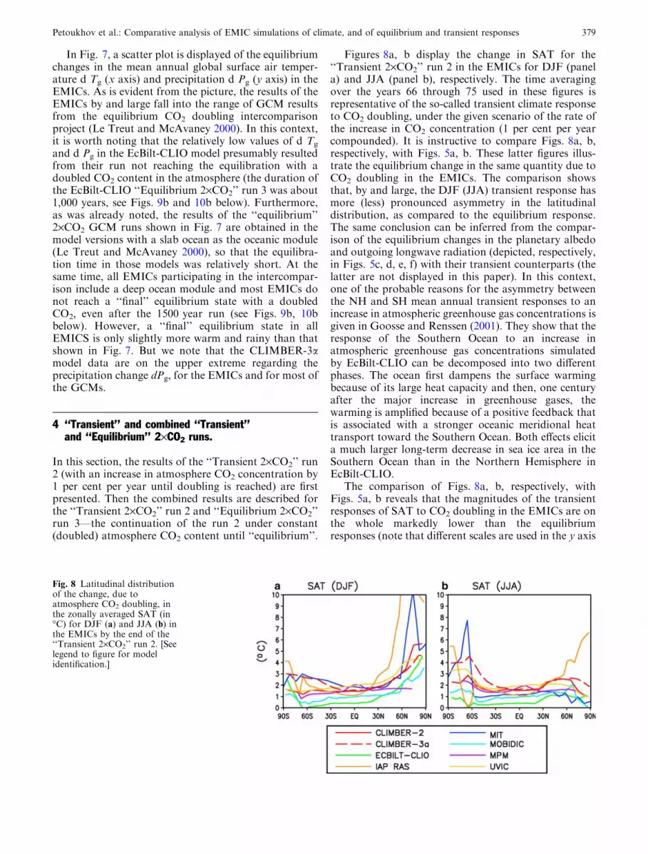
Figures 8a, b display the change in SAT for the‘‘Transient 2·CO2’’ run 2 in the EMICs for DJF (panela) and JJA (panel b), respectively. The time averagingover the years 66 through 75 used in these figures isrepresentative of the so-called transient climate responseto CO2 doubling, under the given scenario of the rate ofthe increase in CO2 concentration (1 per cent per yearcompounded). It is instructive to compare Figs. 8a, b,respectively, with Figs. 5a, b. These latter figures illus-trate the equilibrium change in the same quantity due toCO2 doubling in the EMICs. The comparison showsthat, by and large, the DJF (JJA) transient response hasmore (less) pronounced asymmetry in the latitudinaldistribution, as compared to the equilibrium response.The same conclusion can be inferred from the compar-ison of the equilibrium changes in the planetary albedoand outgoing longwave radiation (depicted, respectively,in Figs. 5c, d, e, f) with their transient counterparts (thelatter are not displayed in this paper). In this context,one of the probable reasons for the asymmetry betweenthe NH and SH mean annual transient responses to anincrease in atmospheric greenhouse gas concentrations isgiven in Goosse and Renssen (2001). They show that theresponse of the Southern Ocean to an increase inatmospheric greenhouse gas concentrations simulatedby EcBilt-CLIO can be decomposed into two differentphases. The ocean first dampens the surface warmingbecause of its large heat capacity and then, one centuryafter the major increase in greenhouse gases, thewarming is amplified because of a positive feedback thatis associated with a stronger oceanic meridional heattransport toward the Southern Ocean. Both effects elicita much larger long-term decrease in sea ice area in theSouthern Ocean than in the Northern Hemisphere inEcBilt-CLIO.

The comparison of Figs. 8a, b, respectively, withFigs. 5a, b reveals that the magnitudes of the transientresponses of SAT to CO2 doubling in the EMICs are onthe whole markedly lower than the equilibriumresponses (note that different scales are used in the y axis

Fig. 8 Latitudinal distributionof the change, due toatmosphere CO2 doubling, inthe zonally averaged SAT (in�C) for DJF (a) and JJA (b) inthe EMICs by the end of the‘‘Transient 2·CO2’’ run 2. [Seelegend to figure for modelidentification.]


in the respective figures). Similar conclusions are validfor the planetary albedo and outgoing longwaveradiation (as well as for P and P�E quantities).

Figure 9a, b shows the time series of the change in themean annual global surface air temperature (GSAT) inEMICs for the ‘‘Transient 2·CO2’’ run 2 (panel a) andin the combined ‘‘Transient’’ and ‘‘Equilibrium’’ 2·CO2

runs 2 and 3 (panel b), beginning with the ‘‘equilibrium’’pre-industrial CO2 state obtained in run 1. As mentionedin Le Treut and McAvaney (2000), a broad range is stillpresent in the AOGCM results on modelling the equi-librium response of GSAT to CO2 doubling in theatmosphere. As can be seen from Fig. 9a, b, for bothruns 2 and 3, the EcBilt-CLIO model somewhat under-estimates the response of GSAT to the increase in theCO2 loading of the atmosphere, as compared to all otherEMICs. The ‘‘equilibrium’’ climate sensitivity, which wedefine, for any EMIC, as the difference between the

average over the last 10 years of integration the globalsurface air temperatures developed in the model by theend of the ‘‘Equilibrium’’ 2·CO2 run 3 and by the end ofthe ‘‘Equilibrium’’ 1·CO2 run 1, is about 1.75�C in theEcBilt-CLIO. Presumably, this relatively low ‘‘equilib-rium’’ climate sensitivity is a consequence of a rather lowsensitivity in the model of the tropical and subtropicalSAT to the atmosphere CO2 content (see Figs. 5a, b, 8a,b). In general, this feature is inherent in the quasi-geo-strophic models, which have a somewhat schematicdescription of the dynamics and thermodynamics of thetropical atmosphere. We note, however, that EcBilt-CLIO does not reach its ‘‘final’’ equilibration with adoubled CO2 content in the atmosphere by the end ofthe 1,000-year ‘‘Equilibrium’’ 2·CO2 run 3 in the model(see Fig. 9b). The UVic model demonstrates the highest‘‘equilibrium’’ climate sensitivity (about 3.6�C), amongthe presented EMICs. The IAP RAS model reveals a

Fig. 9 The time series of thechange in the mean annualglobal SAT (in �C) (a, b) andmaximum value of the NorthAtlantic overturningstreamfunction (in Sv) (c, d),and the time series of the globalsea level rise due to thermalexpansion of sea water (GSLR,in m) (e, f) in the EMICs for the‘‘Transient 2·CO2’’ run 2 (a, c,e) and the combined‘‘Transient’’ and ‘‘Equilibrium’’2·CO2 runs 2 and 3 (b, d, f),beginning with the‘‘equilibrium’’ pre-industrialCO2 state obtained in run 1.The vertical bars in a and closedcircles in b exhibit, respectively,the scatter in the results ofCMIP2 AOGCMs reported inCovey et al. (2003) and thescatter in the results of theequilibrium 2·CO2 response inCMIP2 AOGCMs displayed inCovey et al. (2000). The verticalbar in e marks the uncertaintyin the low and middleprojections of the GSLR in theAMIP GCMs reported in IPCC(1995). The crosses, closedcircles and open circles in e and fdesignate, respectively, thepresented in IPCC (2001)results from the participating inCMIP2 GFDL, HADCM andECHAM AOGCMs, for thecorresponding scenarios of CO2

increase [See legend to figure forEMIC identification. IAP RASis missing in c, d, e, f; MPMmissing for GSLR in e, f, seeTable 3.]


nearly constant response of GSAT (about 2.1�C) to CO2

doubling in the atmosphere after the first 150 years ofintegration. For that reason, the IAP RAS curve is notshown in Fig. 9b. By and large both the transient andequilibrium responses of GSAT to the atmosphere CO2

doubling in the EMICs are within the range of GCMresults (as defined above in the Introduction) from theCMIP2 intercomparison project (see Fig. 9a, b) as de-rived from the results presented by Covey et al. (2000,2003).

Figure 9c, d displays the time evolution of the changein the maximum value of the North Atlantic overturningstreamfunction (MAOSF) for the runs shown in Fig. 9a,b (IAP RAS is missing in Fig. 9c, d, e, f). As seen fromFig. 9c, d, the time series of the change in MAOSF foreach EMIC is characterised by a negative ‘‘kink’’ duringapproximately the first 500 years of the integration,although the amount of the ‘‘kink’’ differs noticeably

from model to model. This behaviour is found inAOGCMs as well. For example, the GFDL AOGCMresponse to the same scenario of atmosphere CO2 in-crease includes changes in the MAOSF which are verysimilar to that found in CLIMBER-2, except that in theGFDL model the magnitude of a ‘‘kink’’ is roughlytwice as large (cf. Fig. 9.25 from IPCC (2001)). It isinteresting to note that, in contrast to all the otherEMICs, the CLIMBER-3a and the UVic models have aMAOSF at 1,500 year which is larger than the initialvalue. Also, the variability of the MAOSF drasticallydecreases in CLIMBER-3a after approximately350 years of integration, probably due to an abruptchange in the total area of the NH polar convection sitesin the model. These are intriguing issues that deserve tobe examined in more detail in the future.

Figure 9e, f is the same as Fig. 9c, d but for global sealevel rise (GSLR) due to thermal expansion of sea water.

Fig. 10 The same as in Fig. 9but for the change in the meanannual global precipitation (inmm/day) (a, b), and sea ice area(in 106 km2) in the NH (c, d)and SH (e, f). The vertical barsin a indicate the range of GCMresults, as derived from thepresented in Covey et al. (2003)temporal trends for the sameclimate characteristics from theCMIP2 AOGCMs. [See legendto figure for modelidentification. IAP RAS ismissing in c, d and e, f; MPMmissing for the NH sea ice areain c, d, see Table 3.]


As can be seen from Fig. 9e, f, the EMIC results areclose to those of the CMIP2 AOGCMs, although in anumber of cases the EMIC values tend to be lower thanthe AOGCM values. It is instructive to comment on thedifference in the simulation of GSLR in CLIMBER-2and CLIMBER-3a: the CLIMBER-2 curves in both theleft and right panels of Fig. 9e, f lie higher than those forCLIMBER-3a. This feature is typical of the model re-sults produced when employing an ocean module withisopycnal mixing (as is in CLIMBER-3a) versus thoseresults for an ocean module with horizontal mixing (asin CLIMBER-2).

Interestingly enough, the global surface air tempera-ture change and the global sea level rise in most EMICsby the end of the ‘‘Transient’’ 2·CO2 run 2 come to onlyone-third to two-thirds their values in the end of the‘‘Equilibrium’’ 2·CO2 run 3 (cf. Figs. 9a, b, e, f), whichreveals a crucial role the deep ocean plays in the Earth’sclimate system response to CO2 change in the atmo-sphere (cf. also Figs. 10a, b).

Figure 10a, b is the same as Fig. 9a, b but for timeseries of the change in the mean annual global precipi-tation. As can be seen from Fig. 10a, b, all the EMICs(except for the IAP RAS and CLIMBER-3a models) fallinto the range of GCM results from the CMIP2 as canbe derived from the results displayed in Covey et al.(2003). After the first 150 years of integration, the IAPRAS model exhibits a nearly constant in time increase inthe mean annual global precipitation (about2.7 mm day�1) in response to CO2 doubling in theatmosphere. For that reason, the IAP RAS curve is notshown in Fig. 10b.

Figure 10c, d, e, f illustrate the time series for thechange in the mean annual sea ice area in the NorthernHemisphere (NHI) and the Southern Hemisphere (SHI)in the EMICs for the same ‘‘Transient 2·CO2’’ run 2(panels c, e) and combined ‘‘Transient’’ and ‘‘Equilib-rium’’ 2·CO2 runs 2 and 3 (panels d, f). MPM is missingdata for the change in NHI in Fig. 10c, d (see Table 3),and hence MPM sea ice data are plotted only inFig. 10e, f. IAP RAS is missing in Fig. 10c, d, e, f. Ascan be seen from Fig. 10c, d, e,f, the dispersion of theEMIC results in modelling the various sea ice covercharacteristics is rather pronounced, and some specificfeatures of the time evolution of the SHI in the EMICsshould be clarified (see Fig. 10f). In particular, in theMoBidiC and MIT models a stepwise structure of thetime evolution of the sea ice area occurs, which could bea consequence of the implementation in these models ofthe zonal averaging formalism and rather coarsemeridional resolution. Such features can manifestthemselves in sudden changes in the ocean mixed layerdepth in what is actually a single grid point, which canresult in the above-mentioned stepwise structure of thetime series of the sea ice area. The CLIMBER-3a modelexhibits a rather high sensitivity of the sea ice area in theSH to CO2 doubling, which presumably could resultfrom the overestimation of the SHI in this EMIC (seeSect. 2).

5 Conclusions

In summary, the performance of EMICs for the equi-librium 280 ppm CO2 climate shows:

– a general qualitative and, in many cases, quantitativeagreement between the modelled and observed fieldsof zonally averaged SAT, planetary albedo, outgoinglongwave radiation, precipitation, and the NorthAtlantic overturning thermohaline circulation

– a scatter in the EMIC results that is by and largewithin the limits of the uncertainty in the results of thepresent-day climate simulations in AMIP AGCMsand CMIP1 AOGCMs

– a modelled direct radiative forcing due to CO2 dou-bling at the top of the atmosphere that is consistentwith that in the AGCMs at the tropopause.

At the same time, some gaps are revealed in theEMIC simulations with regard to the details of the lat-itudinal structure of individual climatic fields. In par-ticular, we note a somewhat overestimated magnitude ofthe simulated seasonal cycle for the zonally averagedlatent heat fluxes due to the synoptic eddies/waves andthe mean meridional circulation, and a large dispersionin the modelled magnitudes and positions of peaks andminima in the latitudinal distribution of zonally aver-aged P�E. Modelling of the global hydrological cycle(especially cloudiness), sea ice concentration and oceanicfreshwater flux remains the weak point in EMICs, aswell as in CMIP1 AOGCMs. Adequate parameterisa-tions have to be developed in the EMICs for thedescription of some explicitly unresolved energy-relatedstructures, e.g. the macro-scale oceanic gyres (in EMICswith zonal oceanic modules), quasi-stationary planetary-scale thermal and orographic atmospheric waves (in themodels with the energy-moisture balance-type atmo-spheric modules) and ENSO.

The performance of the eight EMICs with respect tothe response of the Earth’s climate to an increase in theatmosphere CO2 concentration reveals:

– a general qualitative agreement (among EMICs) onthe overall latitudinal structure of the equilibrium andtransient responses of SAT to CO2 doubling in theatmosphere

– a dispersion of the EMIC results in simulating theequilibrium and transient responses of globally aver-aged SAT and precipitation to CO2 doubling which issimilar to that in CMIP2 AOGCM results

– a scatter of the EMIC results in the phase space of theequilibrium changes in the global surface temperatureand precipitation due to CO2 doubling, which fallsinto the range of AGCM (coupled to a slab ocean)results

– a qualitatively close agreement of the EMIC resultswith those of the CMIP2 AOGCMs in the temporalevolution of the maximum Atlantic overturningstreamfunction due to CO2 doubling


– a qualitatively and quantitatively close agreement ofthe EMIC results with those of the CMIP2 AOGCMsin the character of the time evolution of the global sealevel rise due to CO2 increase, with higher values ofthis characteristics in the EMICs with horizontalmixing and lower values in the models with isopycnalmixing in the ocean module

We thus conclude that EMICs could be successfullyemployed as a useful and highly efficient, in terms of therunning time, tool for the assessment of the long-termsurface air temperature, precipitation and sea levelchanges, under a variety of future and past climatescenarios, as well as for testing and validating differentconcepts and parameterisation schemes for the individ-ual climate mechanisms and feedbacks.

However, a noticeable dispersion is detected in EMICresults as to the latitudinal response to transient andequilibrium CO2 doubling of some important climatecharacteristics, e.g. the zonally averaged planetaryalbedo, outgoing longwave radiation, and P�E. Apronounced quantitative discrepancy is revealed insimulating the CO2-driven changes in the maximumAtlantic overtuning streamfunction and the sea ice areasin the NH and SH. This indicates that the sensitivity ofthe specific climate processes (e.g. the global hydrologi-cal cycle) and feedbacks (e.g. cloud and snow/sea icesurface albedo feedbacks), as well as of their relativestrength, to the external (e.g. anthropogenic) forcingmight differ widely in EMICs. This necessitates furtherintercomparison of EMICs, in particular, with respect tothe efficiency of climate feedbacks operating in theseclimate models. A serious problem for the majority ofEMICs remains the lack of adequate simulation ofinterannual and interdecadal climate variability. In thiscontext, the implementation of the nonstationary partialdifferential equations for treating the atmospheresynoptic-scale eddy/wave ensemble fluxes and variancesis of specific interest.

Acknowledgements The contributions of L.A. Mysak and Z. Wangto this paper were supported by the Canadian Natural Sciences andEngineering Research Council and Canadian Foundation for Cli-mate and Atmospheric Sciences. T. Fichefet and H. Goosse areresearch associates with the Belgian National Fund for ScientificResearch. A.J. Weaver and M. Eby received funding from theCanadian Natural Sciences and Engineering Research Council andCanadian Foundation for Climate and Atmospheric Sciences. I.I.Mokhov and A.V. Eliseev are supported by the Russian Founda-tion for Basic Research (grants 05-05-64907, 05-05-65034 and05-05-65167) and the Russian President Scientific Program (grants1636.2003.5 and 3570.2004.5). M.Montoya is funded by theSpanish Ministry for Science and Education through the Ramon yCajal programme. The authors are indebted to the anonymousreviewers for their constructive comments.

References

Alcamo J, Kreileman GJJ, Leemans R (eds) (1996) Integratedscenarios of global change: results from the IMAGE 2.1 model.Spec Iss Global Environ Change 6(4):255–394

Berlyand TG, Strokina LA (1980) Global distribution of totalcloudiness. Gidrometeoizdat Leningrad, 71 pp

Brovkin V, Ganopolski A, Svirezhev Y (1997) A continuous cli-mate-vegetation classification for use in climate-biospherestudies. Eco Model 101:251–261

Campbell GG, Vonder Haar TH (1980) Climatology of radiationbudget measurements from satellites. Atm Sci Paper No 323,Dept Atmos Sci Colorado State University: 74 pp

Cess RD, Zhang MH, Potter GL, Barker HW, Colman RA,Dazlich DA, Delegenio AD, Esch M, Fraser JR, Galin V, GatesWL, Hack JJ, Ingram WJ, Kiehl JT, Lacis AA, Letreut H, LiZX, Liang XZ, Mahfouf JF, McAvaney BJ, Meleshko VP,Morcrette JJ, Randall DA, Roeckner E, Royer JF, Sokolov AP,Sporyshev PV, Taylor KE, Wang WC, Wetherald RT (1993)Uncertainties in carbon dioxide radiative forcing in Atmo-spheric General Circulation Models. Science 262:1252–1255

Chalikov DV, Verbitsky MYa (1984) A new Earth climate model.Nature 308:609–612

Claussen M, Mysak LA, Weaver AJ, Crucifix M, Fichefet T,Loutre M-F, Weber SL, Alcamo J, Alexeev VA, Berger A,Calov R, Ganopolski A, Goosse H, Lohmann G, Lunkeit F,Mokhov II, Petoukhov V, Stone P, Wang Z (2002) Earth sys-tem models of intermediate complexity: closing the gap in thespectrum of climate system models. Clim Dyn 18:579–586

Colman R, Fraser J, Rotstayn L (2001) Climate feedbacks in ageneral circulation model incorporating prognostic clouds.Clim Dyn 17:103–122

Covey C, Abe-Ouchi A, Boer GJ, Boville BA, Cubasch U, Fair-head L, Flato GM, Gordon H, Guilyardi E, Jiang X, Johns TC,Le Treut H, Madec G, Meehl GA, Miller R, Noda A, PowerSB, Roeckner E, Russel G, Schneider EK, Stouffer RJ, TerrayL, von Storch J-S (2000) The seasonal cycle in coupled ocean-atmosphere general circulation models. Clim Dyn 16:775–787

Covey C, AchutaRao KM, Cubasch U, Jones P, Lambert SJ,Mann ME, Phillips TJ, Taylor KE (2003) An overview of re-sults from the Coupled Model Intercomparison Project. GlobalPlanet Change 37:103–133

Cox PM (2001) Description of ‘‘TRIFFID’’ Dynamical GlobalVegetation Model. Hadley Centre Techn Note HCTN24, Exe-ter, UK

Cox PM, Betts RA, Jones CD, Spall SA, Totterdell IJ (2000)Acceleration of global warming due to carbon-cycle feedbacksin a coupled climate model. Nature 408:184–187

Crucifix M, Loutre MF, Tulkens P, Fichefet T, Berger A (2002)Climate evolution during the Holocene: a study with an Earthsystem model of intermediate complexity. Clim Dyn 19:43–60

Demchenko PF, Velichko AA, Eliseev AV, Mokhov II, NechaevVP (2002) Dependence of permafrost conditions on globalwarming: comparison of models, scenarios, and paleoclimaticreconstructions. Izvestiya, Atmos Ocean Phys 38(2):143–151

Dickinson RE, Henderson-Sellers A, Kennedy PJ, Wilson MF(1986) Biosphere-Atmosphere Transfer Scheme (BATS) for theNCAR Community Climate Model. NCAR/TN-275+STR,NCAR Boulder, Colorado: 69 pp

Dickson RR, Brown J (1994) The production of North Atlanticdeep water: sources, rates and pathways. J Geophys Res99(C6):12319–12341

Dobrolyubov SA (1991) Estimate of the freshwater component ofmeridional water transport in the ocean. Meteorol Gidrol 1:71–78

Eliseev AV, Mokhov II (2003) Amplitude-phase characteristics ofthe annual cycle of surface air temperature in the NorthernHemisphere. Adv Atmos Sci 20(1):1–16

England MH (1993) Representing the global-scale water masses inocean general circulation models. J Phys Oceanogr 23:1523–1552

Ewen TL, Weaver AJ, Eby M (2004) Sensitivity of the inorganicocean carbon cycle to future warming in the UVic coupledmodel. Atmos Ocean 42:23–42

Fichefet T, Morales Maqueda MA (1997) Sensitivity of a global seaice model to the treatment of ice thermodynamics anddynamics. J Geophys Res 102(C6):12609–12646


Fiorino M (1997) A merged surface air temperature data set for thevalidation of AMIP I. PCMDI Web Rep, Lawrence LivermoreNational Laboratory [Available online at http://www-pcmdi.llnl.gov/obs/ipcc/ ]

Gallee H, van Ypersele JP, Fichefet Th, Tricot Ch, Berger A (1991)Simulation of the Last Glacial Cycle be a Coupled, SectoriallyAveraged Climate-Ice Sheet Model 1. The Climate Model. JGeophys Res 96(D7):13139–13161

Ganachaud A, Wunsch C (2000) Improved estimates of globalocean circulation, heat transport and mixing from hydro-graphic data. Nature 408:453–457

Ganopolski AV, Rahmstorf S, Petoukhov VK, Claussen M (1998)Simulation of modern and glacial climates with a coupled glo-bal model of intermediate complexity. Nature 391:351–356

Ganopolski A, Petoukhov V, Rahmstorf S, Brovkin V, ClaussenM, Eliseev A, Kubatzki C (2001) CLIMBER-2: a climate sys-tem model of intermediate complexity. Part II: Model sensi-tivity. Clim Dyn 17:735–751

GatesWL,Mitchell JFB, Boer GJ, Cubasch U,Meleshko VP (1992)Climate modelling, climate prediction and model validation. In:Houghton JT, Callander BA, Varney SK (eds) Climate change.The supplementary report to the IPCC Scientific Assessment,Cambridge University Press, Cambridge, UK, pp 97–134

Gates WL, Boyle JS, Covey C, Dease CG, Doutriaux CM, DrachRS, Fiorino M, Gleckler PJ, Hnilo JJ, Marlais SM, Phillips TJ,Potter GL, Santer BD, Sperber KR, Taylor KE, Williams DN(1999) An overview of the results of the Atmospheric ModelIntercomparison Project (AMIP I). Bull Amer Meteor Soc 80(1):29–55

Goody RM (1964) Atmospheric radiation. I: Theoretical basis.Clarendon Press, Oxford, 436 pp

Goosse H, Renssen H (2001) A two-phase response of the SouthernOcean to an increase in greenhouse gas concentrations. Geo-phys Res Let 28(18):3469–3472

Goosse H, Selten FM, Haarsma RJ, Opsteegh JD (2001) Decadalvariability in high northern latitudes as simulted by an inter-mediate-complexity climate model. Ann Glaciol 33:525–532

Harrison EP, Minnis P, Barkstrom BP, Ramanathan V, Cess RD,Gibson GG (1990) Seasonal variation of cloud radiative forcingderived from the Earth Radiation Budget Experiment. J Geo-phys Res 95:18687–18703

Harvey LDD (1992) A Two-Dimensional Ocean Model for long-term climate simulations: stability and coupling to AtmosphericSea Ice Models. J Geophys Res 97(C6):9435–9453

Hastenrath S (1982) On meridional heat transport in the worldocean. J Phys Oceanogr 12:922–927

Holfort J (1994) Grossramige Zirkulation und meridionale Tran-sporte im Sudatlantik. PhD Dissertation, Institut fur Me-ereskunde, Kiel, Germany

Hsiung J (1985) Estimates of global oceanic meridional heattransport. J Phys Oceanogr 15:1405–1413

Hurrel JW, Campbell GG (1992) Monthly mean global satellitedata sets available in CCM history tape format. NCAR TechNote NCAR/TN-371+STR: 94 pp

IPCC (1990) Climate change: the IPCC scientific assessment. In:Houghton JT, Jenkins GJ, Ephraums JJ (eds) CambridgeUniversity Press, Cambridge, 365 pp

IPCC (1995) Climate Change 1995: the Science of climate change.In: Houghton JT, Meira Filho LG, Callender BA, Harris N,Kattenberg A, Maskel K (eds) Cambridge University Press,Cambridge, 572 pp

IPCC (2001) Climate change 2001: the Scientific Basis. In: HoughtonJT, Ding Y, Griggs DJ, Noguer M, van der Linden PJ, Dai X,Maskell K, Johnson CA (eds) Contribution ofWorking Group Ito the Third Assessment Report of the Intergovernmental Panelon Climate Change. Cambridge University Press, Cambridge,United Kingdom and New Jork, NY, USA, 881 pp

Jager L (1976) Monatskarten des Niederschlags fur die ganze Erde.Ber Deutsche Wetterdienstes 18(139):38

Jennings RL (1975) Data sets for meteorological research. NCARTechnical Note, NCAR-TN/1A, Narional Center for Atmo-spheric Research, Boulder, 156 pp

Jones PD (1988) Hemispheric surface air temperature variations:recent trends and an update to 1987. J Climate 1:654–660

Kalnay E, Kanamitsu M, Kistler R, Collins W, Deaven D, GandinL, Iredel M, Saha S, White G, Woollen J, Zhu Y, Leetmaa A,Reynolds R, Chelliah M, Ebisuzaki W, Higgins W, JanowiakJ, Mo KC, Ropelewski C, Wang J, Jenne R, Joseph D (1996)The NCEP/NCAR 40-year reanalysis project. Bull Amer MetSoc 77:437–471

Kamenkovich I, Sokolov A, Stone P (2002) An efficient climatemodel with a 3D ocean and statistical-dynamical atmosphere.Clim Dyn 19:585–598

Kessler A (1968) Globalbilanzen von Klimaelementen. Ein Beitragzur allgemeinen Klimatologie der Erde. Ber. Inst Meteorol undKlimatol der Techn Univer Hannover No 3

Kim S-J, Flato GM, Boer GJ, McFarlane NA (2002) A coupledclimate model simulation of the Last Glacial Maximum, Part I:transient multi-decadal response. Clim Dyn 19:515–537

Lambert SJ, Boer GJ (2001) CMIP1 evaluation and intercompar-ison of coupled climate models. Clim Dyn 17:83–106

Le Treut H, McAvaney B (2000) A model intercomparison ofequilibrium climate change in response to CO2 doubling. Notesdu Pole de Modelisation de l’IPSL No 18, Institut Pierre SimonLaPlace, Paris, France

Levermann A, Griesel A, Hofmann M, Montoya M, Rahmstorf S(2005) Dynamic sea level changes following changes in thethermohaline circulation. Clim Dyn 24:347–354

Maier-Reimer E, Mikolajewicz U, Hasselmann K (1993) Mean cir-culation of the Hamburg LSG OGCM and its sensitivity to thethermohaline surface forcing. J Phys Oceanogr 23:731–757

Manabe S, Stouffer RJ (1988) Two stable equilibria of a coupledocean-atmosphere model. J Climate 1:841–866

Manabe S, Stouffer RJ (1999) Are two modes of thermohalinecirculation stable?. Tellus 51A:400–411

Mann ME (1998) A Study of Ocean-Atmosphere Interaction andLow-Frequency Variability of the Climate System. PhD Thesis,Yale University, New Haven, CT, 283 pp

Matthews HD, Weaver AJ, Eby M, Meissner KJ (2003) Radiativeforcing of climate by historical land cover change. Geophys ResLett 30(2):Art. No. 1055

Meissner KJ, Weaver AJ, Matthews HD, and Cox PM (2003) Therole of land-surface dynamics in glacial inception: A study withthe UVic Earth System Model. Clim Dyn 21:515–537

Mokhov II, Demchenko PF, Eliseev AV, Khon VCh, Khvo-rost’yanov DV (2002) Estimation of global and regional climatechanges during the 19th-21st centuries on the basis of the IAPRAS model with consideration for anthropogenic forcing. Iz-vestiya Atmos Ocean Phys 38 (5):555–568

Mokhov II, Eliseev AV, Demchenko PF, Khon V Ch, AkperovMG, Arzahnov MM, Karpenko AA, Tikhonov VA, Cher-nokulsky AV, Sigaeva EV (2005) Climate changes and theirassessment based on the IAP RAS global model simulations.Doklady Earth Sci (in press)

Montoya M, Griesel A, Levermann A, Mignot J, Hofmann M,Ganopolski A, Rahmstorf S (2004) The Earth System Model ofIntermediate Complexity CLIMBER-3a. Part I: description andperformance for present day conditions. Clim Dyn (in press)

Oglesby RJ, Saltzman B (1990) Extending the EBM—the effect ofdeep ocean temperature on climate with application to thecretaceous. Glob Plan Change 82 (3–4):237–259

Ohring G, Adler S (1978) Some experiments with a ZonallyAveraged Climate Model. J Atmos Sci 35:186–205

Oka A, Hasumi H, Suginohara N (2001) Stabilization of thermo-haline circulation by wind-driven and vertical diffusive salttransport. Clim Dyn 18:71–83

Oort AH, Rasmusson EM (1971) Atmospheric circulation statis-tics. NOAA Prof Pap 5, Rockville: 323 pp

Opsteegh JD, Haarsma RJ, Selten FM, Kattenberg A (1998) EC-BILT: a dynamic alternative to mixed boundary conditions inocean models. Tellus 50A:348–367

Peixoto JP, Oort AH (1983) The atmospheric branch of thehydrological cycle and climate. In: Variations of the globalwater budget. Reidel, London: 5–65


Petoukhov VK (1980) A zonal climate model of heat and moistureexchange in the atmosphere over the underlying layers of oceanand land In: Golitsyn GS, Yaglom AM (eds) Physics of theatmosphere and the problem of climate. Moscow, Nauka: 8–41(in Russian)

Petoukhov VK (1991) Dynamical-statistical modeling of the large-scale climatic processes. Dr. habil. Thesis, Leningrad Hydro-meteorological Institute, St. Petersburg, 431 pp (in Russian)

Petoukhov VK, Mokhov II, Eliseev AV, Semenov VA (1998) TheIAP RAS Global Climate Model. Dialogue Publishing House,Moscow State University, Moscow, 110 pp

Petoukhov V, Ganopolski A, Brovkin V, Claussen M, Eliseev A,Kubatzki C, Rahmstorf S (2000) CLIMBER-2: A climate sys-tem model of intermediate complexity. Part I: Model descrip-tion and perfomance for present climate. Clim Dyn 16:1–17

Petoukhov V, Ganopolski A, Claussen M (2003) POTSDAM - aset of atmosphere statistical-dynamical models: theoreticalbackground. PIK Report No 81, Potsdam Institute for ClimateImpact Research (PIK), March 2003: 136 pp

Petukhov VK, Feygel’son YM (1973) A model of long-period heatand moisture exchange in the atmosphere over the ocean,Izvestiya Atmos Ocean Phys 9:352–362

Prinn R, Jacoby H, Sokolov A, Wang C, Xiao X, Yang Z, EckhausR, Stone P, Ellerman D, Melillo J, Fitzmaurice J, KicklighterD, Holian G, Liu Y (1999) Integrated global system model forclimate policy assessment: feedbacks and sensitivity studies.Clim Change 41:469–546

Rahmstorf S (1996) On the freshwater forcing and transport of theAtlantic thermohaline circulation. Clim Dyn 12:799–811

Rahmstorf S, Ganopolski A (1999) Long-term global warmingscenarios computed with an efficient coupled climate model.Clim Change 43(2):353–367

Ramanathan V, Lian MS, Cess RD (1979) Increased atmosphericCO2-zonal and seasonal estimates of the effect on the radiationenergy-balance and surface-temperature. J Geophys Res84(C8):4949–4958

Renssen H, Goosse H, Fichefet T (2002) Modeling the effect offreshwater pulses on the early Holocene climate: The influenceof high-frequency climate variability. Paleoceanography 17 (2),DOI 10.1029/2001PA000649

Robock A (1980) The seasonal cycle of snow cover, sea ice andsurface albedo. Mon Wea Rev 108:267–285

Ropelewski CF (1989) Monitoring large-scale cryosphere/atmo-sphere interactions. Adv Space Res 9:213–218

Rossow WB, Schiffer RA (1999) Advances in understanding cloudsfrom ISCCP. Bull Amer Meteor Soc 80:2261–2287

Rossow WB, Garder LC, Lu PJ, Walker AW (1991) InternationalSatellite Cloud Climatology Project (ISCCP): documentation ofcloud data. WMO/TD-No.266, World Meteorological Organi-zation: 76 pp

Saltzman B (1978) A Survey of Statistical-Dynamical Models of theTerrestrial Climate.Advances in Geophysics 20:183–295

Saltzman B, Vernekar AD (1968) A parameterization of the large-scale transient eddy flux of relative angular momentum.MonWea Rev 96(12):854–857

Saltzman B, Vernekar AD (1971) An equilibrium solution for theaxially symmetric component of the earth’s macroclimate.J Geophys Res 76(6):1498–1524

Saltzman B, Vernekar AD (1972) Global Equilibrium Solutionsfor the Zonally Averaged Macroclimate.J Geophys Res77(21):3936–3945

Schiller A (1995) The mean circulation of the Atlantic Ocean northof 30S determined with the adjoint method applied to an oceangeneral circulation model. J Mar Res 53:453–497

SchmittnerA,MeissnerKJ, EbyM,WeaverAJ (2002) Forcing of thedeep ocean circulation in simulations of the Last Glacial Maxi-mum. Paleoceanogr 17, 5:1–5:15 (10.1029 / 2001PA000633)

Schmitz WJ (1995) On the interbasin-scale thermohaline circula-tion. Rev Geophys 33:151–173

Schmitz Jr W, McCartney MS (1993) On the North Atlantic cir-culation. Rev Geophys 13:29–49

Schubert S, Wu C-Y, Zero J, Schemm J-K, Park C-K, Suarez M(1992) Monthly means of selected climate variables for 1985–1989. NASA Techn Memo, Goddard Space Flight Center:376 pp

da Silva AM, Young CC, Levitus S (1994) Atlas of Surface MarineData, Vol 2: Anomalies of Directly Observed Quantities.NOAA Atlas NESDIS 7, U.S. Department of Commerce,Washington DC: 416 pp

Stocker TF, Wright DG, Mysak LA (1992) A zonally averaged,coupled ocean-atmosphere model for paleoclimate studies.J Climate 5:773–797

Stone PH (1972) A Simplified Radiative-Dynamical Model for theStatic Stability of Rotating Atmospheres. J Atmos Sci 29(3):405–418

Stowe LL, Jacobowitz H, Ohring G, Knapp KR, Nalli NR (2002)The Advanced Very High Resolution Radiometer (AVHHR)Pathfinder Atmosphere (PATMOS) climate dataset: Initialanalysis and Evaluation. J Climate 15:1243–1260

Talley LD (1984) Meridional heat transport in the Pacific Ocean.J Phys Oceanogr 14:231–241

Talley LD, Reid JL, Robbins PE (2003) Data-based meridionaloverturning streamfunction for the Global Ocean. J Climate16:3213–3226

Trenberth KE, Solomon A (1994) The global heat balance: heattransport in the atmosphere and ocean. Clim Dyn 10:107–134

Verbitsky MYa, Chalikov DV (1986) Modelling of the Glaciers-Ocean- Atmosphere System. In: Monin AS (ed) Leningrad,Hydrometeoizdat, 133 pp. (in Russian)

Wang Z, Mysak LA (2000) A simple coupled atmosphere-ocean-sea ice-land surface model for climate and paleoclimate studies.J Climate 13:1150–1172

Wang Z, Mysak LA (2002) Simulation of the last glacial inceptionand rapid ice sheet growth in the McGill Paleoclimate Model.Geophys Res Lett, 29(23), 10.1029/2002GL015120

Warren SG, Hahn CJ, London J, Chervin RM, Jenne RL (1986)Global distribution of total cloud cover and cloud typeamounts over the ocean. Technical note tn-273+strNCAR-Boulder, CO42pp.+185 maps

Warren SG, Hahn CJ, London J, Chervin RM, Jenne RL (1988)Global distribution of total cloud cover and cloud typeamounts over land. Technical note tn-273+strNCARBoulder,CO42pp.+200 maps

Weaver AJ, Eby M, Fanning AF, Wiebe EC (1998) Simulatedinfluence of carbon dioxide, orbital forcing and ice sheets on theclimate of the last glacial maximum. Nature 394:847–853

Weaver AJ, Eby M, Wiebe EC, Bitz CM, Duffy PB, Ewen TL,Fanning AF, Holland MM, MacFadyen A, Matthews HD,Meissner KJ, Saenko O, Schmittner A, Wang HX, YoshimoriM (2001) The UVic Earth System Climate Model: modeldescription, climatology, and applications to past and futureclimates. Atmosphere-Ocean 39(4):361–428

Xie P, Arkin P (1997) Global precipitation: A 17-year monthlyanalysis based on gauge observations, satellite estimates,and numerical model outputs. Bull Amer Meteor Soc 78:2539–2558

Zebiak SE, Cane MA (1987) A Model El Nino-Southern Oscilla-tion. Mon Wea Rev 115:2262–2278


Documents

EMIC Intercomparison Project (EMIP–CO2): comparative analysis of EMIC simulations of climate, and of equilibrium and transient responses to atmospheric CO2 doubling