End-to-end delays in polling tree networks

P. Beekhuizen

Philips Research

and

Eurandom

beekhuizen@

eurandom.tue.nl

T.J.J. Denteneer

Philips Research

dee.denteneer@philips.com

J.A.C. Resing

Eindhoven University

of Technology

resing@win.tue.nl

Abstract

We consider a tree network of polling stations operating in discrete-time. Packets arrive

from external sources to the network according to batch Bernoulli arrival processes. We

assume that all nodes have a service discipline that is HoL-based. The class of HoL-based

service disciplines contains for instance the Bernoulli and limited service disciplines, and hence

also the classical exhaustive and 1-limited. We obtain an exact expression for the overall

mean end-to-end delay, and an approximation for the mean end-to-end delay of packets per

source. The study is motivated by Networks on Chips where multiple processors share a single

memory.

1 Introduction

In polling systems multiple queues share a single server, which leads to all kinds of research topicsin performance analysis, optimisation, etc. Polling models have many applications, for examplein telecommunications, transportation, healthcare, etc., and have been the subject of numerousstudies (for surveys, see [19, 20, 22]).

The main application that motivates this study is a Network on Chip (NoC). Networks on Chipsare an emerging paradigm for the connection of on-chip modules like processors and memories.Such modules are traditionally connected via single buses, but because these buses cannot be usedby multiple modules simultaneously, communication difficulties arise as the number of modulesincreases. Networks on Chips have been proposed as a solution (see [9]). In NoCs, routers areused to transmit packets to their destination, so that multiple links can be used at the same timeand communication becomes more efficient.

In particular, we are motivated by a NoC where multiple masters (e.g., processors) share asingle slave (e.g., memory). Packets travel from the processors to the memory over a number ofrouters. Each router has several queues sharing a single link connecting that router to the next.Because the link can be seen as a server attending multiple queues, the router can be seen as apolling station, and the network of routers thus as a network of polling stations.

Although polling systems have been studied extensively, few attempts have been made toanalyse networks of polling servers; one of the rare examples is a heavy-traffic study [13]. Recently,the authors showed in [1] that a tree network of polling systems can be reduced to a single node,while preserving some information on the mean end-to-end delay. This reduction will be discussedin more detail in Section 2.1.

The mean end-to-end delay per source is an important measure for the performance of Networkson Chips. For instance, if this delay is large, it means that processors have to wait a long timebefore data can be written to or read from the memory, which in turn degrades the performanceof the processors.

In this paper, we obtain an exact expression for the mean end-to-end delay averaged over allsources and an approximation of the mean end-to-end delay per source. The essential steps in

1

this approximation are on the one hand the assumption that all streams passing through a certainqueue at a node have the same mean waiting time in that node, and on the other hand applicationof the reduction result of [1].

In the approximation, we express the mean end-to-end delay per source in terms of the meanwaiting time (per queue) in single-station polling systems. Depending on the service disciplinesused, the mean waiting time in these single-station polling systems can either be determinedexactly or has to be approximated.

The reduction result is valid for the class of HoL-based service disciplines. This class containsfor instance the Bernoulli scheduling and mi-limited service disciplines. In this paper, we areespecially interested in polling stations with the 1-limited service discipline, because that disciplinewill prove valuable for Networks on Chips.

This paper is organised as follows: The model is introduced in Section 2. In Section 3, wederive an exact expression for the mean end-to-end delay averaged over all sources, and obtain theapproximation of the mean end-to-end delay per source. We perform a detailed simulation studyon the accuracy of the assumption that all streams passing through a certain queue at a node havethe same mean waiting time in that node in Section 4. The availability of single-station resultsis discussed in more detail in Section 5. For trees with a symmetry property, our approximationassumption becomes exact, as is discussed in Section 6. In Section 7 we combine the mean end-to-end delay approximation of Section 3 with a single-station approximation of Section 5 and applythese to a tree network model of Networks on Chips. We present our conclusions in Section 8.

2 Model

We consider a concentrating tree network operating in discrete time. An example is displayed inFigure 1. All packets and time slots have fixed size 1. Packets arrive from external sources atthe end of time slots in batches according to batch Bernoulli arrival processes. By this we meanthat the number of packets arriving is stochastically identical in each time slot, and independentof what happened in previous time slots. Furthermore, we assume that all arrival processes fromthe external sources are mutually independent.

Node 0

i 1 i 2

i 3 i 4

type i

Figure 1: A polling tree network.

A packet arriving at a node at the end of time slot [t − 1, t), i.e., at time t, may be served intime slot [t, t + 1). In this case it reaches the next node at time t + 1 where it may be served intime slot [t + 1, t + 2), and so on.

All nodes in the network are polling nodes without switch-over times. Node 0 is a node with Nqueues and is the last node of the network (the sink). All packets in the network must eventuallypass through it and leave the network after that.

The service disciplines of all nodes are work-conserving. Besides that, they remain unspecifiedfor the moment; we will make an additional assumption on the service disciplines in Section 2.1.

2

We call a packet that passes through queue i of node 0 a ‘type i’ packet. There are Ni externalsources from which type i packets arrive. We subdivide type i packets into ’type i j’ packets,j = 1, . . . , Ni, such that the type denotes the source from which packets arrive (see Fig. 1). Theset of type i packets is thus the union of the sets of type i j packets.

The size of the batches of type i j packets arriving each time slot is given by an arbitrarydiscrete non-negative random variable, denoted by Xi j . We further define Xi =

∑Ni

j=1 Xi j , andX =

∑

i Xi. Because all packets have size 1, we denote the expected batch sizes by ρi j , ρi, andρ, respectively. We assume ρ < 1 so all nodes are stable.

Every node n in the tree network is itself the last node (the sink) in a smaller tree networkconsisting of all nodes above n and n itself. We call the latter network the node n subtree.

2.1 Reduction to a single node

In [1], it was shown that, under a relatively mild assumption on the service discipline of node 0,an arbitrary tree network can be reduced to a single-station polling system, called the reducedsystem (see Fig. 2). This reduction leaves the mean delay of type i packets invariant; the meanend-to-end delay of type i packets in the original system is equal to the mean waiting time inqueue i of the reduced system. Here, the end-to-end delay of a packet is defined as the sum of itswaiting times at the individual nodes.

The reduced system is a system with arrival processes that are given by superpositions of theoriginal arrival processes, i.e., it is a system with arrivals Xi =

∑

j Xi j to queue i, i = 1, . . . , N .The service discipline of the reduced system is the same as that of node 0 in the original system.

i 1i 2

i 3i 4

type i

Figure 2: The reduced system.

If we denote the end-to-end delay of type i packets by Zi, and the waiting time in queue i ofthe reduced system by W ′

i , we have:E[Zi] = E[W ′

i ]. (2.1)

Equation (2.1) is valid if node 0 uses a so-called Head-of-Line based (HoL-based) service discipline.For the precise definition of HoL-based we refer to [1], but it entails that the server decides whichpacket it is going to serve at time t only based on whether queues are empty or non-empty attimes t, t − 1, . . . , t − M for an arbitrary finite M . It may not, for instance, take queue lengthsinto account. Service disciplines such as longest/shortest queue first are thus not HoL-based.

For the present paper it suffices to say that the class of HoL-based service disciplines includes- but is not limited to - the following two classes of service discplines:

• Bernoulli scheduling, i.e., after serving a packet at queue i, the server serves queue i (if itis non-empty) again with probability pi, and moves to one of the other non-empty queueswith probability 1 − pi;

• mi-limited, i.e., the server serves queue i until it has served mi packets, or the queue becomesempty, whichever happens first, before moving to one of the other non-empty queues.

If the server decides to select one of the other non-empty queues, it may do so according to somefixed order (e.g., a cyclic order) or according to Markovian routing. The exhaustive service policy(i.e., serve queue i until it becomes empty) is a special case of the Bernoulli scheduling, namely

3

pi = 1, and a limiting case of mi-limited, namely mi → ∞. The 1-limited service discipline is aspecial case of both, namely pi = 0 and mi = 1.

The reduction result described here only yields an expression for the mean end-to-end delay oftype i packets (called the mean type i end-to-end delay), while we are in particular interested inthe mean end-to-end delay of type i j packets (called the mean type i j end-to-end delay). Evenso, the reduction result will prove vital for the analysis of the mean type i j end-to-end delay inSection 3. In order to apply the reduction to all possible subtrees, we assume that all nodes useHoL-based service disciplines.

Remark 2.1 The latter assumption can be slightly weakened. We apply the reduction result toall node n subtrees, except for nodes n where all queues store packets arriving directly from theexterior. If one or more queues of node n store packets coming from another node, the servicediscipline of node n has to be HoL-based. If all queues store packets arriving directly from theexterior, the service discipline can be an arbitrary work-conserving one.

3 Analysis of the tree

In this section we describe how the reduction result can be applied to obtain expressions for themean end-to-end delay. First, we obtain an exact expression for the mean end-to-end delay ofpackets of any type, called the mean overall end-to-end delay. Second, we approximate the meantype i j end-to-end delay using the results for the mean overall end-to-end delay.

3.1 Overall end-to-end delay

Recall from Section 2.1, Eq. (2.1), that

E[Zi] = E[W ′i ],

where E[Zi] is the mean type i end-to-end delay, and E[W ′i ] is the mean waiting time in queue i of

the reduced system, which is a polling system with arrivals Xi to queue i, i = 1, . . . , N . Because anarbitrary packet is of type i with probability ρi/ρ, it follows that E[Z], the mean overall end-to-enddelay, is given by

E[Z] =N

∑

i=1

ρi

ρE[Zi] =

N∑

i=1

ρi

ρE[W ′

i ] (3.1)

The right hand side of (3.1) can be recognised as part of the conservation law for pollingsystems [2, 4, 7]. This law states that for any work-conserving service discipline,

N∑

i=1

ρi

ρE[W ′

i ] = C, (3.2)

where C is a constant. For unit packet sizes, C is given by [2, Eq. (14), divided by ρ]:

C =1

2ρ(1 − ρ)

∑

i

E[Xi(Xi − 1)] +∑

i

∑

j 6=i

ρiρj

= −1

2+

1

2ρ(1 − ρ)

∑

i

Var(Xi). (3.3)

By combining this with (3.1) and (3.2), and applying the definition of Xi, we obtain

E[Z] = −1

2+

1

2ρ(1 − ρ)

∑

i

Var(Xi)

= −1

2+

1

2ρ(1 − ρ)

∑

i

∑

j

Var(Xi j) (3.4)

4

as the mean overall end-to-end delay.

Remark 3.1 Equation (3.4) gives the mean overall end-to-end delay, regardless of the preciseHoL-based service discipline. The work of Morrison [12] and Shalmon [16] entails that Equa-tion (3.4) holds without the assumption of HoL-based service disciplines; any work-conservingservice discipline suffices. The assumption of HoL-based service disciplines will, however, becomecrucial in the next subsection. Shalmon [16] also gives an expression for the mean overall end-to-end delay in a concentrating tree network with Poisson arrivals, which is valid in discrete as wellas continuous time (Eq. (3.4) with Var(Xi j) = ρi j).

3.2 End-to-end delay per type

In this subsection, we derive an approximation of the mean type i j end-to-end delay. Our mainresult is that we express the type i j end-to-end delay in the network in the mean waiting timeper queue of single-station polling systems. Although the latter is not always known exactly, weassume that it can somehow be determined, either through exact analysis or approximation. Wewill come back to this issue in Section 5.

The first observation is that the type i j end-to-end delay consists of the sum of the waitingtimes of type i j packets at all nodes along their path from the source to node 0. In other words, ifwe approximate the mean waiting time of type i j packets at an arbitrary node, an approximationof the mean type i j end-to-end delay automatically follows by summing the mean waiting timeapproximations at the individual nodes.

A second observation is the following: Consider Figure 3 and suppose for a moment that wewant to determine the mean waiting time of type i j packets in node i. Everything that happensoutside the node i subtree (marked by the dashes) has no influence on the mean waiting time innode i, so it suffices to consider only the node i subtree. Node i, however, is itself the sink of thenode i subtree. In order to approximate the mean waiting time of type i j packets in an arbitrarynode, it hence suffices to determine the mean waiting time in the last node of an arbitrary network.

In the sequel, we approximate the mean waiting time of type i j packets in node 0, which leadsto an approximation of the mean type i j end-to-end delay as described by the two observations

above. We denote the mean waiting time of type i j packets in node 0 by E[W(0)i j ].

It is not immediately clear, however, how E[W(0)i j ] can be determined: First, it is unclear which

of the type i packets in node 0 are actually type i j packets. The type i j packets are intermingledwith packets of type i j1, i j2, etc. Packets are stored in node 0 in an intricate unknown order

that is determined by the service disciplines of the nodes upstream. Second, E[W(0)i j ] represents

the mean waiting time in a polling model where the arrivals are given by the output of the nodeupstream.

Node 0

i 1 i 2

i 3 i 4

type i

Node iYi

Figure 3: The example network.

5

The first difficulty is circumvented by the following approximation:

Approximation 3.2 At every node, the mean waiting time of type i j packets in that node isequated to the mean waiting of all packets passing through the same queue in that node.

The accuracy of this approximation will be studied numerically in Section 4.Applying Approximation 3.2 to node 0 entails that we approximate the mean waiting time at

node 0 of type i j packets by the mean waiting time of type i packets, i.e.,

E[W(0)i j ] ≈ E[W

(0)i ]. (3.5)

The quantity E[W(0)i ], however, still represents the mean waiting time in a polling model where

arrivals are given by the output of the node upstream.We can now circumvent the second difficulty with the reduction result of Section 2.1: The

mean waiting time of type i packets at node 0, E[W(0)i ], is equal to the mean type i end-to-end

delay in the entire tree, E[Zi], minus the mean type i end-to-end delay in the node i subtree,denoted by E[Yi]. Using the reduction result (Equation (2.1)) we thus obtain

E[W(0)i ] = E[W ′

i ] − E[Yi].

Because all packets in the node i subtree are type i packets, E[Yi] is the mean overall end-to-end delay in the node i subtree. It follows from the analysis of Section 3.1 (i.e., Equation (3.4)applied to the node i subtree) that

E[Yi] = −1

2+

1

2ρi(1 − ρi)

∑

j

Var(Xi j). (3.6)

In summary,

E[W(0)i j ] ≈ E[W

(0)i ] = E[W ′

i ] − E[Yi] (3.7)

where E[Yi] is given by (3.6), and E[W ′i ] is the mean waiting time in queue i of the reduced system.

The two key steps in the derivation of (3.7) are Approximation 3.2 and application of the reductionresult.

Remark 3.3 If type i j packets arrive to node 0 directly, there is of course no suitable subtree.

In this case, we can replace E[Yi] by 0, so that E[W(0)i j ] ≈ E[W

(0)i ] = E[W ′

i ].

4 Accuracy of Approximation 3.2

In this section, we analyse the accuracy of Approximation 3.2 by means of a simulation study overa large parameter space.

Type 1 Type 2

Node 1

Node 0

1 1 1 2

2 1

Figure 4: The network of Section 4.

6

We consider the smallest non-trivial polling tree network, which consists of two nodes, node 0and 1, both with two queues (see Fig. 4). Queue 1 of node 0 stores packets arriving from node 1while queue 2 of node 0 stores packets arriving from the exterior directly. There are three differenttypes of packets, namely type 1 1, type 1 2, and type 2 1. All arrivals occur according to ordinary(non-batch) Bernoulli arrival processes, i.e., each time slot an arrival of type i j takes place withprobability ρi j . We introduce a unit sum weight vector ν = (ν1 1, ν1 2, ν2 1) such that ρi j = νi jρfor a single load parameter ρ. We assume each node uses the 1-limited service discipline.

Without loss of generality, we assume ν1 1 ≤ ν1 2. We cover all possible cases of νi j with astepsize of 0.05 between consecutive values of νi j . This leads to a total of 90 possible cases (seeTable 1). For each case, we run simulations for ρ from 0.01 to 0.99.

Table 1: The 90 cases considered.

Case ν1 1 ν1 2 ν2 1 Case ν1 1 ν1 2 ν2 1

1 0.05 0.05 0.90 35 0.15 0.15 0.70

2 0.05 0.10 0.85 36 0.15 0.20 0.65...

......

......

......

...

18 0.05 0.90 0.05 48 0.15 0.80 0.05

19 0.10 0.10 0.80 49 0.20 0.20 0.60...

......

......

......

...

34 0.10 0.85 0.05 89 0.45 0.45 0.10

90 0.45 0.50 0.05

We analyse the error made in the approximation of the mean waiting time at node 0 (Eq. (3.5)),i.e., we analyse the value of

εj =E[W

(0)1 ]

E[W(0)1 j ]

− 1, j = 1, 2,

where both E[W(0)1 ] and E[W

(0)1 j ] are determined by simulation.

Figure 5 displays the average and extreme values of εj over all cases. It clearly shows that theaverage error is within a few percent for all loads above 0.1. For loads close to 0, εj is the ratioof two numbers close to zero, which leads to some irrelevant variability in the graph. The resultsfor ρ < 0.1 have therefore been omitted from the graph.

0.2 0.4 0.6 0.8 1−0.15

−0.1

−0.05

0

0.05

0.1

0.15

ρ

maximumaverageminimum

j = 1

0.2 0.4 0.6 0.8 1−0.15

−0.1

−0.05

0

0.05

0.1

0.15

ρ

maximumaverageminimum

j = 2

Figure 5: Average and extreme values of εj over all cases.

Apart from average and extreme values of εj , it is interesting to see which cases typicallyinduce large errors. Table 2 shows the five cases that most frequently have large errors; clearly,cases with large errors are typically quite asymmetric. Additional simulations have furthermore

7

0 0.1 0.2 0.3 0.4 0.5 0.6 0.7 0.8 0.9−0.02

−0.01

0

0.01

0.02

0.03

0.04

ν1 2 − ν1 1

ε1

ε2

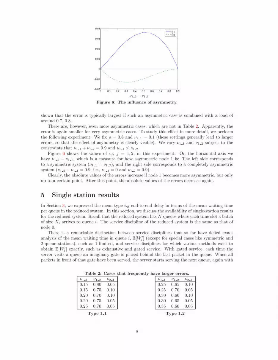
Figure 6: The influence of asymmetry.

shown that the error is typically largest if such an asymmetric case is combined with a load ofaround 0.7, 0.8.

There are, however, even more asymmetric cases, which are not in Table 2. Apparently, theerror is again smaller for very asymmetric cases. To study this effect in more detail, we performthe following experiment: We fix ρ = 0.8 and ν2 1 = 0.1 (these settings generally lead to largererrors, so that the effect of asymmetry is clearly visible). We vary ν1 1 and ν1 2 subject to theconstraints that ν1 1 + ν1 2 = 0.9 and ν1 1 ≤ ν1 2.

Figure 6 shows the values of εj , j = 1, 2, in this experiment. On the horizontal axis wehave ν1 2 − ν1 1, which is a measure for how asymmetric node 1 is: The left side correspondsto a symmetric system (ν1 1 = ν1 2), and the right side corresponds to a completely asymmetricsystem (ν1 2 − ν1 1 = 0.9, i.e., ν1 1 = 0 and ν1 2 = 0.9).

Clearly, the absolute values of the errors increase if node 1 becomes more asymmetric, but onlyup to a certain point. After this point, the absolute values of the errors decrease again.

5 Single station results

In Section 3, we expressed the mean type i j end-to-end delay in terms of the mean waiting timeper queue in the reduced system. In this section, we discuss the availability of single-station resultsfor the reduced system. Recall that the reduced system has N queues where each time slot a batchof size Xi arrives to queue i. The service discipline of the reduced system is the same as that ofnode 0.

There is a remarkable distinction between service disciplines that so far have defied exactanalysis of the mean waiting time in queue i, E[W ′

i ] (except for special cases like symmetric and2-queue stations), such as 1-limited, and service disciplines for which various methods exist toobtain E[W ′

i ] exactly, such as exhaustive and gated service. With gated service, each time theserver visits a queue an imaginary gate is placed behind the last packet in the queue. When allpackets in front of that gate have been served, the server starts serving the next queue, again with

Table 2: Cases that frequently have larger errors.

ν1 1 ν1 2 ν2 1

0.15 0.80 0.050.15 0.75 0.100.20 0.70 0.100.20 0.75 0.050.25 0.70 0.05

Type 1 1

ν1 1 ν1 2 ν2 1

0.25 0.65 0.100.25 0.70 0.050.30 0.60 0.100.30 0.65 0.050.35 0.60 0.05

Type 1 2

8

an imaginary gate behind the last packet, and so on.In [14], it is shown that service disciplines satisfying a well-known ‘branching property’ can be

exactly analysed. This branching property states the following:

Property 5.1 If the server arrives to queue i and finds ki packets there, then during the courseof the server’s visit, all of these ki packets are effectively replaced in an i.i.d. manner by anN -dimensional random population.

For instance, with exhaustive service, all type i packets will have been removed (i.e., replaced by0 packets) once the server moves to the next queue, whereas for j 6= i, as many type j packets willbe added to queue j as there are arriving during one type i busy period (i.e., every type i packetis replaced by the packets arriving to the other queues during a type i busy period). Likewise,with gated service, for all j, including j = i, every type i packet will be replaced by the packetsarriving during a type i service. In contrast, with the 1-limited service discipline one type i packetis replaced by packets arriving during the type i service, but all other type i packets are leftunchanged (i.e., replaced by one type i packet). Hence, the 1-limited service discipline does notsatisfy the branching property.

For service disciplines satisfying the branching property, it is shown in [14] that the number ofpackets in different queues, embedded at time points where the server visits queue 1, constitutesa multi-type branching process (MTBP) with immigration. Furthermore, it is mentioned that theclass of MTBPs is one of the exceptional classes of multi-dimensional Markov chains for which theequilibrium distribution can be determined.

This at least partially explains why methods exist to obtain mean queue lengths (and thus meanwaiting times) for exhaustive and gated service disciplines. Nevertheless, even for these servicedisciplines, E[W ′

i ] is, apart from special cases such as symmetric systems, not given explicitly butin terms of a matrix inverse, infinite product, or a solution to a set of equations.

We are in particular interested in HoL-based service disciplines for which E[W ′i ] can be obtained

exactly. Gated service, however, is not HoL-based. With the gated service discipline an imaginarygate is placed behind packets in the queue, so the decision to serve a particular queue at time tmay depend on the queue lengths before t, which is not allowed for HoL-based service disciplines.

Exhaustive service, on the other hand, is HoL-based. The mean queue lengths in a pollingstation with exhaustive service can be found in [15] and [18], where it is given in terms of a solutionto a system of equations. Although the expressions given there are still implicit, E[W ′

i ] can bedetermined numerically from them.

In the remainder of this section, we give explicit results for symmetric stations, and we give anapproximate result for the 1-limited service discipline. The latter will be particularly importantin Section 7.

5.1 Symmetric stations

In this subsection, we obtain exact results for symmetric stations. Throughout this subsection,

we assume all arrival processes are stochastically identical: Xjd= X1 for all j.

We first introduce the concept of symmetric service disciplines: We define a service disciplineto be symmetric if it satisfies the following three properties: First, if the server is at a queueit serves a number of packets there according to a fixed rule such as 1-limited, exhaustive, orBernoulli service. This rule is the same for all queues. Second, Markovian routing is used, whichmeans that after service of queue j, the server moves to queue k 6= j with probability pjk. Third,the routing matrix P = (pjk) is circulant, i.e.,

P =

0 p2 p3 . . . pN

pN 0 p2 . . . pN−1

pN−1 pN 0 . . . pN−2

......

. . ....

p2 p3 p4 . . . 0

, (5.1)

9

or can be written in circulant form after a permutation of the queues. Note that cyclic routinghas a circulant P -matrix with p2 = 1.

Suppose that the reduced system uses a service discipline with a circulant P -matrix. Then all

rows of P are identical, apart from being shifted. Because, in addition, Xjd= X1 for all j, there

is no difference between the various queues, i.e., the mean waiting times per queue are invariantunder permutation of the queues. Similarly, if the P -matrix is not circulant but can be written incirculant form, it can also be argued that the mean waiting times per queue are invariant underpermutation of the queues.

Because the mean waiting times per queue are invariant under permutation, we have E[W ′i ] =

E[W ′1] for all i. It thus follows from the conservation law (3.2) that E[W ′

i ] is exactly given by

E[W ′i ] = C = −

1

2+

1

2ρ(1 − ρ)NVar(X1),

for all i, regardless of the precise service discipline, as long as it is symmetric.

5.2 1-limited

We give the approximation proposed by Boxma and Meister [6] for 1-limited polling systems.Although their analysis is aimed at continuous-time systems, it can easily be established that thekey steps in their derivation are valid for discrete-time systems as well.

The Boxma-Meister approximation states that

E[W ′i ] ≈ C

1 − ρ + ρi

1 − ρ + 1ρ

∑

j ρ2j

,

where C is again the constant of the conservation law (3.3). The Boxma-Meister approximationhas the two following properties: (i) It is exact for symmetric systems, and (ii) its numericalaccuracy degrades for heavily loaded and very asymmetric systems.

In particular, if the 1-limited service discipline is used, all queues receive a positive fractionof the capacity of the server, even if the load is larger than 1. As a result, some queues remainstable even though others become unstable (see e.g., [8, 11]). The Boxma-Meister approximationdoes not deal with this well; if ρ tends to 1, C tends to infinity so the approximations of all queuesbecome unbounded.

As a refinement to their approximation, Boxma and Meister suggest in [5] that for heavilyloaded, very asymmetric systems, a group of heavily loaded queues can be replaced by a suitableswitch-over time. Although this generally increases the accuracy of the approximation for suchcases, we will see in Section 7.2 that the approximation presented here is accurate for loads up to0.7, even in quite asymmetric systems.

Many other approximations have been suggested (for instance, Blanc [3], Groenendijk andLevy [10], Srinivasan [17], and Van Vuuren and Winands [21]), that might perform better insome cases. However, they generally lack an accessible closed-form expression like that of theBoxma-Meister approximation. Furthermore, transferring their derivations to discrete-time modelsoften involves subtleties. In this paper, we therefore restrict our attention to the Boxma-Meisterapproximation.

6 Symmetric trees

Approximation 3.2 states that all packets passing through the same queue at a node are assumedto have the same mean waiting time at that node. In this section, we introduce a class of treesfor which Approximation 3.2 is in fact not an approximation but an exact statement.

We say that a polling tree is symmetric if it satisfies all of the following five properties:

1. All external arrival processes are stochastically identical.

10

2. All external arrivals occur at the same level. Here, the level of a node is defined as thedistance to the sink.

3. All nodes within a particular level have the same number of queues.

4. All nodes within a particular level use the same service discipline.

5. All nodes use a symmetric service discipline.

Now consider an arbitrary polling tree network, let node i be the node directly above queue i ofnode 0, and suppose that the node i subtree is symmetric. An example of such a tree is displayedin Figure 7.

Given that the entire node i subtree is symmetric, it follows that there is no distinction betweenthe type i j packets, j = 1, . . . , Ni. In particular, the mean waiting time of type i j packets atnode 0 is invariant under permutation of j:

E[W(0)i j ] = E[W

(0)i ].

Approximation 3.2 is thus an exact statement rather than an approximation for node 0. Becauseall subtrees within the node i subtree are again symmetric, Approximation 3.2 is exact for allnodes in the node i subtree.

Moreover, the mean end-to-end delay of type i j packets is invariant under permutation of j.We thus obtain:

E[Zi j ] = E[Zi] = E[W ′i ],

where Zi j is the end-to-end delay of type i j packets, and W ′i is the waiting time in queue i of the

reduced system. If, furthermore, exact results are available for the reduced system (for instanceif it is a symmetric node or if it uses exhaustive service), the mean type i j end-to-end delay canbe obtained exactly.

. . . type i j . . .

Node 0

Node i

Level 2

Level 1

Queue i

Figure 7: A tree with a symmetric node i subtree

Note that there is no condition on nodes outside the node i subtree; all conditions apply tothe node i subtree, and all other nodes (including node 0) are arbitrary.

7 Networks on Chips

In this section, we study a network model based on a Network on Chip. In Section 7.1, wedescribe the network in more detail and combine the approximations of Section 3 and Section 5to approximate the mean type i j end-to-end delay. In Section 7.2 we analyse the accuracy of thecombination of these approximations numerically.

11

7.1 Description

We study a model of a Network on Chip with multiple routers (nodes), as depicted in Figure 8.All traffic has the same destination, motivated by Networks on Chips with a single memory.

The routers in this network are organised in a mesh topology; all routers have four queues andare placed on a lattice (2 × 2 in this case) with connections in four directions (up, down, right,left) if possible. The routing mechanism of this network is XY-routing, which means that packetsfirst traverse the X-direction, as far as they have to go, and then move in the Y -direction to theirdestination. This entails there is in fact a link between node 3 and node 1, but it is never usedbecause all traffic is headed to node 0. It is thus the particular routing strategy that ensures themesh topology is a tree network corresponding to the setting of this paper.

ρ2 3 ρ2 2

ρ2 4 ρ2 1

ρ1 1 ρ3 1

ρ1 2

Node 3 Nd. 2

Nd. 1 Nd. 0

Figure 8: A NoC with 4 routers and 7 input streams

Routers in NoCs often employ wormhole routing, which has two implications: First, once thefirst packet of a batch starts transmission at a certain node, the entire batch has to completetransmission before another batch may start transmission. The second implication of wormholerouting is that if a batch consisting of multiple packets is being transmitted, one packet of thebatch is transmitted to the next router each time slot. These packets might start transmission atthe next router immediately (for instance if that router is empty). Multiple packets of a singlebatch might thus be spread out over several nodes. As a result, a batch of size K that never hasto wait completes transmission over L nodes in L + K − 1 time slots, rather than LK in networkswithout wormhole routing.

Inside routers batches are served according to round-robin scheduling, which means a batch isserved from queue 1, then queue 2, etc. We assume batches have fixed size K, so that wormholerouting is mimicked by the cyclic K-limited service discipline.

We furthermore assume a batch of size K arrives each time slot with probability λi j , so

Xi j =

{

0 w.p. 1 − λi j ,K w.p. λi j ,

andVar(Xi j) = K2λi j(1 − λi j).

Because ρi j = E[Xi j ], it follows that λi j = ρi j/K.We define the waiting time (and end-to-end delay) of a batch to be the waiting time (end-to-

end delay) of the first packet in that batch (the header). In the remainder, we use an additionalsubscript h to indicate headers.

We now approximate the mean waiting time of a type i j header in node 0, denoted by E[W(0)i j,h].

As in Section 3, we do so by reducing the network to a single node, called the reduced system.

12

The reduced system, like node 0, uses K-limited service. Because the batch sizes are fixed andequal to K, the mean waiting time of a header in the reduced system is equal to the mean waitingtime of a packet in a 1-limited system with deterministic service times equal to K and ordinary(non-batch) Bernoulli arrival processes with parameter λi j .

By applying the Boxma-Meister approximation to the latter system, we obtain

E[W ′i,h] ≈

1 − ρ + ρi

1 − ρ + 1ρ

∑

j ρ2j

CK , (7.1)

as an approximation of the mean waiting time of headers in queue i of the reduced system. Here,CK is the constant of the conservation law in a system with non-batch Bernoulli arrivals withparameter λi j and fixed service times equal to K. From [2, Eq. (14), divided by ρ], we get aftersome rewriting:

CK =ρ

2(1 − ρ)

K −∑

i

∑

j

(

ρi j

ρ

)2

. (7.2)

Suppose now that i = 3 (the case i = 1, 2 is slightly different and will be dealt with later).Type 3 1 packets arrive to node 0 directly from the exterior, so the mean waiting time of a headeris equal to that of an arbitrary packet minus (K − 1)/2. The mean waiting time of a header innode 0 (and hence its mean end-to-end delay) is thus given by

E[W(0)3 1,h] = E[W

(0)3 1] −

K − 1

2= E[W ′

3] −K − 1

2= E[W ′

3,h],

where E[W ′3,h] is given by (7.1).

Suppose now that i = 1, 2. Due to the wormhole routing, the header always arrives at node 0one time slot earlier than the second packet, and it always leaves one time slot earlier. Themean waiting time of a header is thus equal to the mean waiting time of an arbitrary packet,

E[W(0)i j,h] = E[W

(0)i j ]. We obtain (cf. Eq. (3.7))

E[W(0)i j,h] = E[W

(0)i j ] ≈ E[W

(0)i ] = E[W ′

i ] − E[Yi],

where E[Yi] is given by (3.6). The quantity E[W ′i ] is the mean waiting time of an arbitrary packet

in the reduced system, which is equal to the mean waiting time of a header plus (K − 1)/2, so

E[W ′i ] = E[W ′

i,h] +K − 1

2

with E[W ′i,h] as in (7.1).

As in Section 3, the mean waiting times in the other nodes can be obtained similarly, resultingin an approximation of the mean end-to-end delay of type i j batches.

7.2 Numerical results

In this subsection we study the performance of the mean end-to-end delay approximation for thefollowing two cases: Balanced load division and homogeneous load division. We again assumethere is a unit sum weight vector ν describing the division of the total load ρ over the variousinput streams, i.e., ρi j = νi jρ.

Case I: Balanced load division

By balanced load division we mean that the loads are divided in such a way that at each node allqueues receive the same load. That is, we assume ν3 1 = 1/3, ν1 1 = ν1 2 = 1/6, ν2 1 = ν2 2 = 1/9,and ν2 3 = ν2 4 = 1/18. Because the corresponding arrival rates are equal, the mean type 1 1end-to-end delay is equal to the mean type 1 2 end-to-end delay. Figure 9 shows mean type 1 i

13

end-to-end delay, i = 1, 2, and Figure 10 the mean type 3 1 end-to-end delay. The approximationsof these types are the most and least accurate, respectively, of all approximations.

0 0.2 0.4 0.6 0.8 10

10

20

30

40

50

60

ρ

SimApprox

Figure 9: The mean type 1 1 and 1 2 end-

to-end delay.

0 0.2 0.4 0.6 0.8 10

10

20

30

40

50

60

ρ

SimApprox

Figure 10: The mean type 3 1 end-to-end

delay.

It is clear that the approximation of the mean end-to-end delay is very accurate in this case.This is not very surprising, as all nodes are almost symmetric. For instance, if we apply thereduction result, we obtain a polling system with three queues, each with load ρ/3. One ofthese queues has an arrival process that is the superposition of four arrival processes (namely∑

j X2 j), one arrival process is a superposition of two (∑

j X1 j), and one is not a superposition(or a superposition of one). In other words, the loads to all queues are identical, but the arrivalprocesses are superpositions of different Bernoulli arrival processes.

Other than this difference, the system is symmetric, in which case the Boxma-Meister ap-proximation is exact. It is indeed unlikely that such a small asymmetry leads to large errors.Furthermore, we already saw in Section 4 that Approximation 3.2 is very accurate if the individ-ual nodes are nearly symmetric.

Case II: Homogeneous load division

With the homogeneous load division, all input streams receive a fraction 1/7 of the total load,i.e., νi j = 1/7. Again, we show the most accurate approximation (Fig. 11, type 2 1 and 2 2), andthe least accurate approximation (Fig. 12, type 3 1).

0 0.2 0.4 0.6 0.8 10

10

20

30

40

50

60

ρ

SimApprox

Figure 11: The mean type 2 1 and 2 2

end-to-end delay.

0 0.2 0.4 0.6 0.8 10

10

20

30

40

50

60

ρ

SimApprox

Figure 12: The mean type 3 1 end-to-end

delay.

We see that up to a load of roughly 0.7, the approximations are very accurate. Beyond thisload, the approximation is only accurate for the input stream with the highest load. This can beexplained by the fact that node 0 is rather asymmetric. After all, one queue receives a fraction of

14

4/7 of the total load, while the other queues get fractions 2/7 and 1/7 respectively. In Section 5we already mentioned that for asymmetric systems, the Boxma-Meister approximation tends toinfinity if ρ tends to 1, even though some queues are still stable. We see this phenomenon too inFigure 12: The mean end-to-end delay approximation is unbounded, whereas the simulated meandelay is still bounded if the load is 1. Other single-station approximations than that of Boxmaand Meister might lead to more accurate results here.

8 Conclusion

Under the assumption that all nodes use HoL-based service disciplines, we have derived an exactexpression for the mean overall end-to-end delay and an approximation for the mean type i jend-to-end delay. The key steps in this approximation were: Equating the mean waiting time oftype i j packets in a node to that of all packets passing through the same queue at that node(Approx. 3.2), and application of the reduction result of [1]. These two steps combined result inan expression for the mean type i j end-to-end delay in terms of the mean waiting time per queuein single-station polling systems.

For the 1-limited service discipline, Approximation 3.2 is very accurate over the entire parame-ter space of the smallest non-trivial tree. It is especially accurate for nearly symmetric systems andextremely asymmetric systems, and somewhat less accurate for moderately asymmetric systems.

In the special case that the subtree directly above queue i is symmetric, Approximation 3.2becomes an exact statement rather than an approximation. If, in addition, exact results areavailable for the reduced system, the mean end-to-end delay per source can be determined exactly.

We applied the approximation for the mean end-to-end delay per type to a model based on aNetwork on Chip using the Boxma-Meister approximation [6] to obtain the necessary single-stationresults. Although the Boxma-Meister approximation is less accurate for asymmetric systems, wecould still accurately approximate the mean type i j end-to-end delay up to moderately high loads(around 0.7) in an asymmetric case study.

Other single-station approximations than that of Boxma and Meister are known, but theyare often less accessible and transferring such approximations to discrete-time models usuallyinvolves subtleties. Depending on the precise characteristics of the tree (e.g., nearly symmetric,very asymmetric, etc.) these other approximations may lead to more accurate results. If the meanend-to-end delay approximation is applied to specific trees, one has to choose which single-stationapproximation to use based on the characteristics of the tree in order to obtain the most accurateresults.

References

[1] P. Beekhuizen, T. Denteneer, and J. Resing. Reduction of a polling network to a single node.Queueing Systems, 58(4):303–319, April 2008.

[2] C. Bisdikian. A note on the conservation law for queues with batch arrivals. IEEE Transac-tions on Communications, 41(6):832–835, June 1993.

[3] J. Blanc. An algorithmic solution of polling models with limited service disciplines. IEEETransactions on Communications, 40(7):1152–1155, July 1992.

[4] O. Boxma and W. Groenendijk. Waiting times in discrete-time cyclic-service systems. IEEETransactions on Communications, 36(2):164–170, February 1988.

[5] O. Boxma and B. Meister. Waiting-time approximations for cyclic-service systems withswitch-over times. ACM SIGMETRICS Performance Evaluation Review, 14(1):254–262, May1986.

[6] O. Boxma and B. Meister. Waiting-time approximations in multi-queue systems with cyclicservice. Performance Evaluation, 7:59–70, 1987.

15

[7] H. Bruneel and B. Kim. Discrete Time Models for Communication Systems including ATM.Kluwer Academic Publishers, Norwell, MA, 1993.

[8] R. Chang and S. Lam. A novel approach to queue stability analysis of polling models.Performance Evaluation, 40:27–46, 2000.

[9] W. Dally and B. Towles. Route packets, not wires: on-chip interconnection networks. InProc. of the 38th Design Automation Conference, pages 684–689, 2001.

[10] W. Groenendijk and H. Levy. Performance analysis of transaction driven computer systemsvia queueing analysis of polling models. IEEE Transactions on Computers, 41(4):455–466,April 1992.

[11] O. Ibe and X. Cheng. Stability conditions for multiqueue systems with cyclic service. IEEETransactions on Automatic Control, 33(1):102–103, January 1988.

[12] J. Morrison. A combinatorial lemma and its application to concentrating trees of discrete-timequeues. The Bell Systems Technical Journal, 57(5):1645–1652, May-June 1978.

[13] M. Reiman and L. Wein. Heavy traffic analysis of polling systems in tandem. OperationsResearch, 47(4):524–534, July 1999.

[14] J. Resing. Polling systems and multitype branching processes. Queueing Systems, 13:409–426,1993.

[15] I. Rubin and L. de Moraes. Message delay analysis for polling and token multiple-accessschemes for local communication networks. IEEE Journal on Selected Areas in Communica-tions, 1:935–947, 1983.

[16] M. Shalmon. Exact delay analysis of packet-switching concentrating networks. IEEE Trans-actions on Communications, 35(12):1265–1271, December 1987.

[17] M. Srinivasan. An approximation for mean waiting times in cyclic server systems with nonex-haustive service. Performance Evaluation, 9:17–33, 1988.

[18] H. Takagi. Analysis of Polling Systems. MIT Press, Cambridge, Massachusetts, 1986.

[19] H. Takagi. Queueing analysis of polling models: an update. In H. Takagi, editor, StochasticAnalysis of Computer and Communication Systems, pages 267–318. North-Holland, 1990.

[20] H. Takagi. Queueing analysis of polling models: progress in 1990-1994. In J. Dshalalow,editor, Frontiers in Queueing: Models and Applications in Science and Engineering, pages119–146. CRC Press, Boca Raton, 1997.

[21] M. van Vuuren and E. Winands. Iterative approximation of k -limited polling systems.Queueing Systems, 55(3):161–178, March 2007.

[22] V. Vishnevskii and O. Semenova. Mathematical methods to study the polling systems. Au-tomation and Remote Control, 67(2):173–220, February 2006.

16