Embed Size (px)
Citation preview
En vue de l'obtention du
DOCTORAT DE L'UNIVERSITÉ DE TOULOUSEDélivré par :
Institut National Polytechnique de Toulouse (INP Toulouse)Discipline ou spécialité :
Génie Electrique
Présentée et soutenue par :M. GABRIEL KHOURYle mardi 16 janvier 2018
Titre :
Unité de recherche :
Ecole doctorale :
Energy efficiency improvement of a squirrel-cage induction motor throughthe control strategy
Génie Electrique, Electronique, Télécommunications (GEET)
Laboratoire Plasma et Conversion d'Energie (LAPLACE)Directeur(s) de Thèse :
M. MAURICE FADELM. RAGI GHOSN
Rapporteurs :M. BABAK NAHID-MOBARAKEH, UNIVERSITÉ LORRAINE
M. GUY CLERC, UNIVERSITE LYON 1
Membre(s) du jury :M. LUC LORON, UNIVERSITE DE NANTES, Président
M. MAURICE FADEL, INP TOULOUSE, MembreMme FLAVIA KHATOUNIAN, UNIVERSITE ST JOSEPH DE BEYROUTH, MembreM. RAGI GHOSN, ECOLE SUPERIEURE D'INGENIEURS BEYROUTH, Membre


iii
To my dear parents.

iv
A diamond is a chunk of coal that did well under pressure
Henry Kissinger

v
Acknowledgments
I would like in the first place to express my deep gratitude to my directors Pr. Maurice
FADEL and Pr. Ragi GHOSN for their vital help and continuous guidance throughout the
whole thesis, as well as my advisor Dr. Flavia KHATOUNIAN for always providing the
necessary advices on the technical and personal levels. Calling you directors and advisors
doesn’t give the complete image, since you were more like family. You were always ready to
help despite all your occupations, but also always there to encourage and boost my motivation
again and again.
I would also like to thank M. Mathias TIENTCHEU for providing the work with all
possible information and equipment from Leroy Somer to enhance the industrial value of the
results. Moreover, I would like to express my appreciation to the committee members, Pr. Guy
CLERC and Pr. Babak NAHID-MOBARAKEH, for accepting to evaluate my thesis report and
for sharing your valuable comments and positive feedback, as well as Pr. Luc LORON for
granting me the honor of presiding the committee and presenting valued remarks.
Special thanks also to the CODIASE team in the LAPLACE laboratory, especially Pr.
Pascal MAUSSION, Pr. Maria DAVID and Pr. Stephane CAUX, for their advice and help in
many issues throughout the thesis during my stays at Toulouse, as well as for the welcoming
and friendly environment created inside the team.
This thesis wouldn’t have been accomplished without the support of the Research Council
and the CINET research center of the Université Saint-Joseph de Beyrouth (USJ), the Agence
Universitaire de la Francophonie AUF, the Lebanese National Council for Scientific Research
CNRS-L, the LAPLACE research center and Leroy Somer – Nidec Industry. These entities and
programs are deeply thanked for supporting the thesis with all necessary funds.
In every situation through these long years, friends were an essential ingredient that kept
things going. I am really thankful for each and every one for making it a pleasant experience.
Thank you for my lab friends Antoine, Leopold, Abdelkader, Khaled, Pedro and Julien for
sharing difficulties in Toulouse and turning them into funny stories. Very special thanks for
my Lebanese friends at Toulouse Bernard, Hiba, Sabina, Sirena, Charbel, Carole… who made
me always feel at home and enjoy every moment outside my country. Thank you for my ESIB
friends and colleagues Melhem, Jean, Samer, Michel and all the REDOC team who
accompanied every step of the process by sharing personal experience and being perfect

vi
listeners when needed! And of course, I can’t forget my old friends who were always there
since before my Ph.D. and always encouraged my decisions… thank you Sergio, Elio, Mario,
Eliane, Freddy, Marianne, Sarah, Christophe, Robert, Yassin, Stephan, André, Wissam… The
list doesn’t end here, many are the friends who were there making my experience special, I
thank you deeply.
In the end, the biggest thanks go to my dear family, Amale, Joe and Christian, who
always believed in my capabilities and encouraged my ambitions especially throughout these
three years, despite all the financial problems we’ve been through. For you I am so grateful,
especially for my dearest Ammoula my super-mum, my weakness and my support in life.

vii
viii
Abstract
Energy efficiency optimization of electric machines is an important research field and is
part of the objectives of several international projects such as the European Commission
Climate and Energy package which has set itself a 20% energy savings target by 2020, and was
extended for 2030 with higher targets. Therefore, this thesis proposes an efficiency
optimization method of the Induction Machine (IM) through the variation of the control
parameters. To achieve this goal, the flux in the airgap is modified according to an optimal flux
table computed off-line for all possible operating points.
The flux table is calculated with the best possible accuracy through an improved dynamic
model of the IM, developed in these works. The latter avoids the main drawback of the classic
dynamic model, by considering the effect of core losses. The core loss model established by
Bertotti is used. It depends on the frequency and the amplitude of the magnetic field. The losses
are then represented by a variable resistor, continuously evaluated according to the operating
point.
The established optimal flux table is a function of the operating conditions in terms of
torque and speed. Indeed, the results show that the flux can be optimized for torque values less
than about half the rated torque, and that this threshold is influenced by the speed. The proposed
optimization method is simulated, then tested for the scalar control and the field-oriented
control, in order to show the genericity of the proposed approach. The validation is carried on
an experimental test bench for two 5.5 kW induction motors of different efficiency standards
(IE2 and IE3). The results obtained show the reduction of the losses in the motor, thus an
improvement of the overall efficiency while preserving a satisfactory dynamic behavior.
Consequently, the optimization of the energy efficiency is validated for the two control
structures and for the two studied motors. In addition to the validation of the simulation results,
the proposed approach is compared to existing methods to assess its effectiveness.
ix
Résumé
L’optimisation de l’efficacité énergétique des machines électriques constitue un domaine
de recherche bien développé et fait partie des objectifs de plusieurs accords internationaux
comme le projet Energie-Climat de la Commission Européenne visant l’amélioration de 20%
d’efficacité pour 2020, encore étendu pour 2030 avec des objectifs plus importants. Ainsi, cette
thèse propose un procédé d’optimisation du rendement du moteur asynchrone en agissant sur
les paramètres du contrôle. Pour atteindre cet objectif, le flux dans l’entrefer est adapté selon
un tableau de flux optimal calculé hors ligne pour tous les points de fonctionnement possibles.
Ce flux est déterminé avec le plus haut degré de précision possible en se basant sur un
modèle dynamique de la machine développé dans ces travaux. Ce dernier pallie le point faible
du modèle dynamique classique, en prenant en compte l’effet des pertes fer. Le modèle des
pertes fer utilisé est celui de Bertotti, qui les évalue en fonction de la fréquence et de l’amplitude
du champ magnétique. Les pertes sont alors représentées par une résistance variable,
continuellement évaluée selon le point de fonctionnement.
Le tableau de flux optimal obtenu est fonction des conditions d’opération repérées dans
le plan couple-vitesse. Ainsi l’étude montre que le flux peut être optimisé pour des valeurs de
couple sensiblement inférieures à environ la moitié du couple nominal, ce seuil variant en
fonction de la vitesse. La méthode d’optimisation proposée est simulée puis testée pour le
contrôle scalaire et le contrôle vectoriel indirect par orientation de flux rotorique, afin de
montrer la généricité de l’approche. La validation est conduite sur une maquette expérimentale
d’une puissance de 5.5 kW et pour 2 machines asynchrones de générations différentes (IE2 et
IE3). Les résultats obtenus montrent la réduction des pertes dans la machine et donc une
amélioration du rendement global, tout en préservant un comportement dynamique satisfaisant.
L’optimisation de l’efficacité énergétique est ainsi validée pour les deux structures de contrôle
et pour les deux types de machine. Outre une comparaison avec la simulation, la solution
proposée est comparée aux méthodes existantes afin d’en apprécier l’efficacité.
Pour plus de détails, un résumé long est disponible à la page 119.

x
Table of Contents
Acknowledgments ............................................................................................................ v
Abstract ........................................................................................................................ viii
Résumé ............................................................................................................................ ix
Table of Contents ............................................................................................................ xi
List of Figures ................................................................................................................ xv
List of Tables .............................................................................................................. xviii
List of Symbols ............................................................................................................. xix
General Introduction ........................................................................................................ 1
Chapter 1 Context of the Thesis .................................................................................... 3
Introduction .................................................................................................................. 4
1.1 General Context................................................................................................ 4
1.1.1 European Climate & Energy Package .......................................................... 4
1.1.2 Energy Efficiency Standards for Electric Motors ......................................... 5
1.2 State of Art of Existing Induction Motors Models ........................................... 7
1.2.1 Steady State Equivalent Circuits .................................................................. 7
1.2.2 Dynamic Model ............................................................................................ 9
1.2.3 Improved Dynamic Models ........................................................................ 13
1.3 Models of the Main Losses ............................................................................ 14
1.3.1 Copper Losses............................................................................................. 15
1.3.2 Mechanical Losses ...................................................................................... 15
1.3.3 Core Losses................................................................................................. 16
1.3.4 Inverter Losses ............................................................................................ 17
1.3.5 Summary ..................................................................................................... 20
1.4 Energy Efficiency Optimization of the Induction Motor ............................... 21
1.4.1 Search Control ............................................................................................ 22
1.4.2 Loss Minimization Control ......................................................................... 23
1.4.3 Maximum Torque per Ampere ................................................................... 24
1.4.4 Summary ..................................................................................................... 25
Conclusion .................................................................................................................. 25
Chapter 2 Induction Motor Model Taking Core Losses into Account ........................ 26
Introduction ................................................................................................................ 27
Table of Contents
xii
2.1 Model Parameters Measurement .................................................................... 27
2.1.1 Mechanical Parameters ............................................................................... 27
2.1.2 Electrical Parameters .................................................................................. 28
2.1.3 Core Losses Model Coefficients ................................................................. 30
2.2 Including Core Losses in the IM Model ........................................................ 31
2.2.1 Equivalent Torque Approach...................................................................... 32
2.2.2 Equivalent Resistor Approach .................................................................... 32
2.2.3 Summary and Analysis ............................................................................... 34
2.3 Including Variable Core Losses ..................................................................... 37
2.3.1 Enhancement of the Improved Dynamic Model ......................................... 38
2.3.2 Simulation Results and Experimental Validation ....................................... 38
Conclusion .................................................................................................................. 39
Chapter 3 Best Efficiency Point Tracking ................................................................... 40
Introduction ................................................................................................................ 41
3.1 Efficiency Computation ................................................................................. 41
3.1.1 Improved Dynamic Model in Complex Form ............................................ 41
3.1.2 Efficiency Equations ................................................................................... 43
3.2 Efficiency Mapping ........................................................................................ 45
3.2.1 Energy Efficiency Curves ........................................................................... 45
3.2.2 Energy Efficiency Plans ............................................................................. 48
3.3 Efficiency Optimization Approach ................................................................ 50
3.3.1 Optimal Flux ............................................................................................... 50
3.3.2 Load Torque Observer ................................................................................ 53
Conclusion .................................................................................................................. 55
Chapter 4 Control Systems Optimization.................................................................... 56
Introduction ................................................................................................................ 57
4.1 Scalar Control Optimization........................................................................... 57
4.1.1 Classic Scalar Control Structure ................................................................. 57
4.1.2 Optimized Scalar Control ........................................................................... 59
4.1.3 Simulation and analysis .............................................................................. 61
4.2 Optimized Field-Oriented Control ................................................................. 67
Table of Contents
xiii
4.2.1 Classic field-oriented Control Structure ..................................................... 67
4.2.2 Optimized field-oriented Control ............................................................... 73
4.2.3 Simulation and analysis .............................................................................. 73
Conclusion .................................................................................................................. 78
Chapter 5 Experimental Validations ........................................................................... 79
Introduction ................................................................................................................ 80
5.1 Experimental Test Bench ............................................................................... 80
5.1.1 Global Test Bench ...................................................................................... 80
5.1.2 Power Elements .......................................................................................... 81
5.1.3 Sensors and Control System ....................................................................... 85
5.1.4 Operating Points Validation ....................................................................... 87
5.2 Optimized Scalar Control Tests ..................................................................... 87
5.2.1 Setup ........................................................................................................... 88
5.2.2 Experimental Results .................................................................................. 89
5.3 Optimized Field-oriented Control Tests ......................................................... 96
5.3.1 Setup ........................................................................................................... 96
5.3.2 Experimental Results .................................................................................. 98
5.4 Comparison with the Existing Optimization Methods ................................. 104
5.4.1 Methods in Literature ............................................................................... 104
5.4.2 Industrial Method ..................................................................................... 106
5.5 IE3 motor tests ............................................................................................. 110
5.5.1 Tested Motor............................................................................................. 110
5.5.2 Experimental Results ................................................................................ 111
5.5.3 Comparison with the IE2 Motor ............................................................... 114
Conclusion ................................................................................................................ 115
General Conclusion ...................................................................................................... 116
Résumé Long en Français ............................................................................................ 119
Introduction .................................................................................................................. 119
Chapitre 1 Contexte de la thèse ................................................................................. 120
1.1 Contexte Général .......................................................................................... 120
1.2 Etat de l’Art des Modèles de la Machine Asynchrone ................................. 121
Table of Contents
xiv
1.3 Modèles des Pertes Principales .................................................................... 124
1.4 Amélioration de l’Efficacité Energétique de la Machine Asynchrone ........ 125
Chapitre 2 Modèle dynamique prenant en compte les pertes fer............................... 125
2.1 Détermination des Paramètres de la Machine .............................................. 126
2.2 Prise en Compte des Pertes Fer .................................................................... 126
2.3 Prise en Compte du Caractère Variable des Pertes Fer ................................ 129
Chapitre 3 Rendement Optimal ................................................................................. 130
3.1 Calcul du Rendement ................................................................................... 130
3.2 Cartographie du Rendement ......................................................................... 130
3.3 Approche d’Optimisation ............................................................................. 132
Chapitre 4 Contrôles Optimisés ................................................................................. 133
4.1 Contrôle Scalaire Optimisé .......................................................................... 133
4.2 Contrôle Vectoriel Optimisé ........................................................................ 134
Chapitre 5 Validation Expérimentale ........................................................................ 139
5.1 Montage Expérimental ................................................................................. 139
5.2 Validation des Contrôles Optimisés ............................................................. 140
5.3 Comparaison avec les Méthodes Existantes................................................. 143
Conclusion .................................................................................................................... 145
References .................................................................................................................... 147
List of Publications ....................................................................................................... 154
Appendix A – Efficiency and Flux Calculation Methods ............................................ 155
Appendix B – Motors Characteristics .......................................................................... 157
Appendix C – Datasheets ............................................................................................. 159
List of Figures
Fig. 1.1. IE efficiency classification according to IEC 60034-30-1:2014 standard [4] ............. 6Fig. 1.2. IM partial leakage inductances equivalent circuit referred to the stator ...................... 8Fig. 1.3. IM global leakage inductance equivalent circuit referred to the stator ....................... 8Fig. 1.4. Dynamic model representation including core losses through equivalent resistor and
inductance ......................................................................................................................... 13Fig. 1.5. d-q dynamic model representation including core losses through equivalent resistor
.......................................................................................................................................... 14Fig. 1.6. Losses in an inverter fed squirrel-cage induction motor system ............................... 15Fig. 1.7. Comparison between SC and intelligent SC flux reference ...................................... 23Fig. 1.8. MTPA strategy reference curves for a 7.5kW IM ..................................................... 24Fig. 2.1. IM speed variation in zero-load deceleration experiment ......................................... 28Fig. 2.2. IM dynamic model schematic representation ............................................................ 33Fig. 2.3. IM dynamic model schematic representation including core losses through an
equivalent resistor ............................................................................................................. 33Fig. 2.4. Simulated core losses in a direct start-up test at 0.25p.u. load .................................. 35Fig. 2.5. Simulated input power in a direct start-up test at 0.25p.u. load ................................ 36Fig. 2.6. Simulated electromagnetic torque in a direct start-up test at 0.25p.u. load ............... 37Fig. 2.7. Simulated speed in a direct start-up test at 0.25p.u. load .......................................... 37Fig. 2.8. Simulated and experimental core losses .................................................................... 38Fig. 3.1. Energy efficiency variations at 0.1p.u. torque ........................................................... 46Fig. 3.2. Energy efficiency variations at 0.3p.u. torque ........................................................... 46Fig. 3.3. Energy efficiency variations at 0.5p.u. torque ........................................................... 47Fig. 3.4. Energy efficiency variations at 1p.u. torque .............................................................. 47Fig. 3.5. Energy efficiency variations in flux-speed plan at 0.1p.u. torque ............................. 48Fig. 3.6. Energy efficiency variations in flux-speed plan at 0.3p.u. torque ............................. 48Fig. 3.7. Energy efficiency variations in flux-speed plan at 0.5p.u. torque ............................. 49Fig. 3.8. Energy efficiency variations in flux-speed plan at 1p.u. torque ................................ 49Fig. 3.9. Optimal stator flux values per load torque and speed requirements .......................... 51Fig. 3.10. Optimal rotor flux values per load torque and speed requirements ......................... 52Fig. 3.11. First order Luenberger load torque observer ........................................................... 54Fig. 3.12. Torque observer simulation ..................................................................................... 55Fig. 4.1. Classic Scalar Control Structure ................................................................................ 58Fig. 4.2. Optimized Scalar Control Structure .......................................................................... 61Fig. 4.3. Simulation of the inverter PWM ............................................................................... 62Fig. 4.4. Optimized scalar control – stator flux reference and actual values ........................... 63Fig. 4.5. Scalar control – speed and electromagnetic torque ................................................... 64Fig. 4.6. Scalar control – Input power and losses. a- copper losses, b- core losses, c- input
power, d- energy efficiency .............................................................................................. 65Fig. 4.7. Scalar control – Input power (zoom) ......................................................................... 66Fig. 4.8. Scalar control – Energy efficiency ............................................................................ 66
List of Figures
xvi
Fig. 4.9. Scalar control – Energy efficiency (zoom) ................................................................ 67
Fig. 4.10. Basic indirect field-oriented control structure ......................................................... 69
Fig. 4.11. FOC speed loop ....................................................................................................... 71
Fig. 4.12. Flux reference reduction .......................................................................................... 72
Fig. 4.13. Approximate IM schematic representation taking core losses into account ........... 72
Fig. 4.14. Flux reference generator – optimized FOC ............................................................. 73
Fig. 4.15. Optimized field-oriented control – rotor flux reference and actual values .............. 74
Fig. 4.16. Field-oriented control – speed and electromagnetic torque ..................................... 75
Fig. 4.17. Field-oriented control – Input power and losses. a- copper losses, b- core losses, c- input power, d- energy efficiency ..................................................................................... 76
Fig. 4.18. Field-oriented control – Input power (zoom) .......................................................... 77
Fig. 4.19. Field-oriented control – Energy efficiency .............................................................. 77
Fig. 4.20. Field-oriented control – Energy efficiency (zoom) ................................................. 78
Fig. 5.1. Test bench structure ................................................................................................... 81
Fig. 5.2. Test bench .................................................................................................................. 81
Fig. 5.3. Semikron inverter. a- didactic block, b- IGBT SKM 50 module, c- SKHI 22 driver83
Fig. 5.4. Leroy Somer IE2 squirrel-cage induction motor LSES 132...................................... 83
Fig. 5.5. Front panel of the dSpace controller.......................................................................... 86
Fig. 5.6. Experimental validation operating points. a- industrial test points, b- effective test points ................................................................................................................................ 87
Fig. 5.7. Optimized scalar control block diagram .................................................................... 89
Fig. 5.8. Experimental scalar control optimization with variable load profile. a- load torque, b- stator flux, c- energy efficiency ........................................................................................ 90
Fig. 5.9. Optimized scalar control operating conditions. a- flux reference, b- speed, electromagnetic and load torque ....................................................................................... 92
Fig. 5.10. Simulated and experimental optimized scalar control results. a- copper losses, b- core losses, c- input power, d- energy efficiency ..................................................................... 93
Fig. 5.11. Simulated and experimental optimized scalar control results (zoom). a- input power, b- energy efficiency .......................................................................................................... 94
Fig. 5.12. Optimized scalar control efficiency increase - IE2 motor ....................................... 96
Fig. 5.13. Optimized field-oriented control block diagram ..................................................... 97
Fig. 5.14. Experimental FOC optimization with variable load profile. a- load torque, b- stator flux, c- energy efficiency .................................................................................................. 98
Fig. 5.15. Optimized FOC operating conditions. a- rotor flux, b- speed and torque ............... 99
Fig. 5.16. Simulated and experimental optimized FOC results. a- copper losses, b- core losses, c- input power, d- energy efficiency .............................................................................. 100
Fig. 5.17. Simulated and experimental optimized FOC results (zoom). a- input power, b- energy efficiency ........................................................................................................................ 101
Fig. 5.18. Optimized FOC efficiency increase - IE2 motor ................................................... 102
Fig. 5.19. Flux variation test – 0.5p.u. speed, 0.25p.u. torque. a- rotor flux, b- energy efficiency ........................................................................................................................................ 103
List of Figures
xvii
Fig. 5.20. Search control technique. a- rotor flux, b- energy efficiency ................................ 104
Fig. 5.21. Intelligent search control technique. a- rotor flux, b- energy efficiency ............... 105
Fig. 5.22. Proposed optimization technique. a- rotor flux, b- energy efficiency ................... 106
Fig. 5.23. Industrial drives optimization curve ...................................................................... 107
Fig. 5.24. Comparison with the industrial optimization – 0.25p.u. speed, 0.5p.u. torque. a- flux, b- energy efficiency ........................................................................................................ 108
Fig. 5.25. Comparison with the industrial optimization - 1p.u. speed, 0.25p.u. torque. a- flux, b- energy efficiency ........................................................................................................ 108
Fig. 5.26. Comparison with the industrial optimization – 0.9p.u. speed, 0.5p.u. torque. a- flux, b- energy efficiency ........................................................................................................ 109
Fig. 5.27. Comparison with the industrial optimization – efficiency improvements ............ 110
Fig. 5.28. Optimized scalar control efficiency increase – IE3 motor .................................... 113
Fig. 5.29. Optimized FOC efficiency increase – IE3 motor .................................................. 114
Fig. 5.30. Comparison IE2 and IE3 motors – 0.9p.u. speed, 0.25p.u. torque. a- IE2 motor, b- IE3 motor ........................................................................................................................ 115
Fig. 1.1. Schéma monophasé étoile équivalent ramené au stator de la machine asynchrone 122
Fig. 2.1. Représentation schématique du modèle dynamique de la machine asynchrone prenant en compte les pertes fer .................................................................................................. 127
Fig. 2.2. Simulation des modèles dynamiques proposés. a- vitesse, b- couple électromagnétique ........................................................................................................................................ 128
Fig. 2.3. Pertes fer expérimentales et simulées ...................................................................... 129
Fig. 3.1. Courbes de rendement. a- couple 0.1p.u., b- couple 1p.u. Abaques de rendement dans le plan flux-vitesse. c- couple 0.1p.u., d- couple 1p.u. ................................................... 131
Fig. 3.2. Abaque de flux statorique optimal........................................................................... 132
Fig. 4.1. Contrôle scalaire optimisé ....................................................................................... 134
Fig. 4.2. Contrôle vectoriel indirect optimisé ........................................................................ 136
Fig. 4.3. Simulation de l’optimisation du flux rotorique dans le cas du contrôle vectoriel ... 137
Fig. 4.4. Simulation de l’effet de l’optimisation proposée sur la vitesse et le couple électromagnétique .......................................................................................................... 137
Fig. 4.5. Simulation de l’effet de l’optimisation proposée sur les pertes et la puissance absorbée. a- pertes Joule, b- pertes fer, c- puissance absorbée, d- pertes onduleur ........................ 138
Fig. 4.6. Simulation de l’effet de l’optimisation proposée sur le rendement ......................... 139
Fig. 5.1. Montage expérimental ............................................................................................. 140
Fig. 5.2. Résultats expérimentaux de l’essai de variation de charge avec et sans optimisation. a- couple de charge, b- flux rotorique, c- rendement. .................................................... 141
Fig. 5.3. Résultats expérimentaux d’augmentation du rendement ......................................... 142
Fig. 5.4. Résultats expérimentaux de variation du flux ......................................................... 143
Fig. 5.5. Résultats expérimentaux d’amélioration du rendement par rapport à l’approche d’optimisation industrielle .............................................................................................. 144
List of Tables Table 1.1. Conduction voltage drops per inverter leg .............................................................. 18
Table 1.2. Power losses ............................................................................................................ 21
Table 3.1. Optimal stator flux table – IE2 motor ..................................................................... 51
Table 3.2. Optimal rotor flux table – IE2 motor ...................................................................... 52
Table 5.1. Studied IE2 motor parameters ................................................................................ 84
Table 5.2. Optimized scalar control experimental vs simulated efficiency error - IE2 motor 95
Table 5.3. Optimized scalar control efficiency increase - IE2 motor ...................................... 95
Table 5.4. Optimized FOC experimental vs simulated efficiency error - IE2 motor ............ 102
Table 5.5. Optimized FOC efficiency increase - IE2 motor .................................................. 102
Table 5.6. Comparison with the industrial optimization – efficiency improvements ............ 109
Table 5.7. Studied IE3 motor parameters .............................................................................. 111
Table 5.8. Optimal stator flux table – IE3 motor ................................................................... 112
Table 5.9. Optimal rotor flux table – IE3 motor .................................................................... 112
Table 5.10. Optimized scalar control efficiency increase – IE3 motor ................................. 113
Table 5.11. Optimized FOC efficiency increase – IE3 motor ............................................... 113
Tableau 3.1. Flux statorique optimal ..................................................................................... 132
Table 1. Studied IE2 motor parameters ................................................................................. 157
Table 2. Studied IE3 motor parameters ................................................................................. 157
Table 3. DC generator parameters ......................................................................................... 158

List of Symbols
magnetic field variable core losses branch subscript , rotating reference frame subscripts voltage frequency � viscous friction coefficient current variable RMS current voltage
total motor and load inertia eddy currents effect core losses coefficient � excess core losses coefficient � hysteresis effect core losses coefficient
Luenberger factor partial stator leakage inductance ′ partial rotor leakage inductance referred to the stator eddy currents inductance magnetizing inductance of the partial leakage inductances equivalent
circuit magnetizing inductance of the global leakage inductance equivalent circuit
stator self-inductance rotor self-inductance magnetizing branch subscript
stator-rotor mutual inductance ′ global leakage inductance referred to the stator core losses � input active power � input reactive power
mechanical losses � rotor copper losses � stator copper losses resistance of a stator phase winding ′ resistance of a rotor phase winding referred to the stator
core losses equivalent resistance short-circuit resistor of the IM equivalent circuit
rotor resistance stator resistance
number of pole pairs of the motor , stator and rotor subscripts dry friction torque core losses equivalent torque
electromagnetic torque load torque
List of Symbols
xx
observed load torque voltage variable
conduction losses voltage drop switching losses voltage drop
RMS stator voltage � switching frequency triangular voltage VSD Variable Speed Drive variable phasor: = +
short-circuit reactance of the IM equivalent circuit short-circuit impedance of the IM equivalent circuit , stationary reference frame subscripts � energy efficiency � motor dispersion coefficient � = − 2
∅ flux variable � mechanical speed of the rotor � electrical speed of the rotor � angular speed of the rotating frame � angular frequency of the rotor currents � angular frequency of the stator currents
General Introduction
The present thesis aims to optimize the energy efficiency of a squirrel-cage induction
motor by acting on the control strategy and fixing the best efficiency operating point.
Energy efficiency optimization has become nowadays the goal of a lot of research, especially for electrical systems, which constitute an essential domain and have significant energy requirements. The European Commission for instance, has set energy efficiency targets, and standards to be reached throughout 2020 and 2030, thus motivating further developments in the field. Indeed, this work is a contribution in fulfilling the objectives of the European project by acting on the energy efficiency optimization of electrical structures.
The squirrel-cage Induction Motor (IM) is a main element among electrical systems since it is one of the most used motors in industry for the simplicity of its installation and use. Indeed, the IM is found in a wide number of industries like construction, transportation, HVAC, packaging, raw materials exploitation, etc. Therefore, the present study is focused on this type of motors.
On the other hand, control systems have a significant role in enhancing the energy efficiency and are therefore an important tool in this domain. Several types of control structures can be used. This thesis focuses on the scalar control, which is used by a wide number of applications for its simplicity, as well as the field-oriented control also widely used for its precision and stability. The energy optimization of these control structures is achieved by acting on the flux reference to change the operating point of the motor.
In order to conduct an efficiency study and to identify the optimal flux, it is essential to analyze the main losses in the system. However, the greater number of studies carried on the induction motor take into consideration copper and mechanical losses, while omitting the core losses because of the complexity of their estimation. Nevertheless, these are main losses which must be addressed to reach the best possible accuracy. For this purpose, the commonly used IM dynamic model that omits core losses is updated in this study to match the requirements.
Several improvement methods relative to efficiency optimization are discussed in literature, and are proved to optimize the efficiency. These methods however lack accuracy in some cases and lead to unsatisfactory dynamic performances in other cases. They are nevertheless used as comparative optimization techniques in this study.
In this thesis, an improved dynamic model of the IM introducing the core losses effect is established, considering their dependency on frequency and magnetic field. This model is then

General Introduction
2
used to analyze the efficiency variations and compute the optimal flux values which are stored in a look-up table. The latter is used to optimize both scalar and field-oriented control structures to reach the best efficiency point. The flux reference is modified throughout the motor operation. In the end, results are simulated and experimentally validated and compared to existing optimization methods to show the originality and effectiveness of the proposed solution. This approach has an industrial vocation for rapid implementation on several types of motors.
In the first chapter, the European Commission project headlines are described especially concerning the efficiency standards, then an overview of the existing induction motor models is presented, as well as a list of the system losses models necessary for the study. A state-of-art of the optimization methods found in literature is presented at the end, showing the advance in the field and the weaknesses to be resolved in the proposed approach.
In the second chapter, the improved dynamic model of the IM taking into account the effect of core losses is presented, along with the necessary parameters measurements. Two methods are presented and compared, then the chosen approach is enhanced by considering the magnetic field and frequency effect of the core losses to improve accuracy.
In the third chapter, the improved dynamic model is used to compute the optimal stator and rotor flux values, which are stored in the look-up table, to be used later in the control structures. Efficiency variations are observed in torque-speed planes to analyze the effect of the operating conditions in terms of flux, torque and speed on the efficiency.
In the fourth chapter, the optimal flux look-up table is used to enhance the scalar and field-oriented controls. The classic and improved control structures are described, and simulation results are presented to confirm the predicted efficiency increase compared to the classic structures results.
In the fifth chapter, experimental validations are presented. A test bench built in the LAPLACE laboratory is described in this section, as well as the series of tests carried to validate the results of both improved control structures. In addition, tests done with existing optimization methods and on a second motor compliant with a better efficiency standard, are presented to prove the originality and effectiveness of the proposed approach.
Chapter 1 Context of the Thesis
Table of Contents
Introduction .................................................................................................................. 4
1.1 General Context................................................................................................ 4
1.1.1 European Climate & Energy Package .......................................................... 4
1.1.2 Energy Efficiency Standards for Electric Motors ......................................... 5
1.2 State of Art of Existing Induction Motors Models ........................................... 7
1.2.1 Steady State Equivalent Circuits .................................................................. 7
1.2.2 Dynamic Model ............................................................................................ 9
1.2.3 Improved Dynamic Models ........................................................................ 13
1.3 Models of the Main Losses ............................................................................ 14
1.3.1 Copper Losses............................................................................................. 15
1.3.2 Mechanical Losses ...................................................................................... 15
1.3.3 Core Losses................................................................................................. 16
1.3.4 Inverter Losses ............................................................................................ 17
1.4 Energy Efficiency Optimization of the Induction Motor ............................... 21
1.4.1 Search Control ............................................................................................ 22
1.4.2 Loss Minimization Control ......................................................................... 23
1.4.3 Maximum Torque per Ampere ................................................................... 24
1.4.4 Summary ..................................................................................................... 25
Conclusion .................................................................................................................. 25

Chapter 1. Context of the thesis
4
Introduction
The optimization of energy efficiency in industrial applications using electrical motors
is a favorite area for studies associated to international projects and standards promoting
‘green’ energies. The squirrel-cage induction motor is one of the most studied systems and the
object of this thesis, since it is widely used in industry and constitutes an important source of
energy consumption. Therefore, several optimization techniques of the IM are proposed in
literature to optimize their efficiency. These studies require the use of mathematical models of
the IM and the losses that occur in the system.
In the present chapter, the general context of this work is presented as part of the
European Commission project goals. The progress in the field is also detailed in terms of motor
and power losses models as well as the state-of-art of the optimization techniques leading to
the method proposed in the thesis, and used as comparative approaches in the rest of the study.
1.1 General Context
Energy efficiency optimization is the main scope of much research nowadays because of
the climate changes and the necessity to reduce energy consumption and promote sustainable
strategies. For this purpose, the European Climate and Energy package of the European
Commission has been established in 2008 along with several standards and projects.
1.1.1 European Climate & Energy Package
The consequences of the 2008 worldwide economic crisis were severe for the progress
of many countries, and exposed the weaknesses in their economic structures, which required
an immediate intervention to ensure a quick recovery. Therefore, the European Union took the
initiative in the ‘Europe 2020 strategy’ [1] and set objectives to be reached by 2020 at different
levels with three priorities: smart, sustainable and inclusive growth.
To this end, a list of headline targets was imposed to promote research and education,
improve the economy, reduce poverty and unemployment, and deal with the climate change
challenges by encouraging sustainable energies and optimizing energy efficiency. The 3*20

Chapter 1. Context of the thesis
5
Climate & Energy package is established to define the three main objectives of the sustainable
energy program as shown below:
• Reduce the greenhouse gas emissions by at least 20% compared to 1990 levels or
by 30%, according to the capabilities of the countries,
• Increase by 20% the use of renewable energy sources for the final energy
consumption,
• Reach a 20% increase in energy efficiency of electric structures.
The scopes of the European project are mutually reinforced, in a way that each objective
helps in achieving the others. For instance, the 3*20 package contributes in adding around 1
million new jobs and increasing the GDP by using the European energy market. Moreover, a
major factor for limiting the greenhouse gas emissions lies in the efficiency optimization of the
energy resources, which makes the latter an important research domain aiming to reach the
climate/energy set goals.
Further to the above, the Climate and Energy package is being updated continuously [2]
and is not only limited to 2020. Targets have already been set for 2030 with 40% cuts in
greenhouse gas emissions (from 1990 levels), 27% share for renewable energy and 27%
improvement in energy efficiency.
The present work is a contribution in the third objective of the Climate & Energy
package, with the aim to optimize the energy efficiency of induction motors. For this purpose,
the targets defined by the European Commission in terms of IM efficiency standards are
explored.
1.1.2 Energy Efficiency Standards for Electric Motors
Since most of the electrical structures are based on electric motors working for several
hours per day, specific guidelines have been established by the European Commission [3]
fixing efficiency targets for manufactured three-phase squirrel-cage induction motors which:
• have 2 to 6 poles,
• have a rated voltage up to 1000 V,
• have a rated power output between 0,75 kW and 375 kW,
Chapter 1. Context of the thesis
6
• are rated for continuous duty operation.
Efficiency standards IE1 to IE4 were set by the International Electrotechnical
Commission (IEC) in the IEC 60034-30-1 standard [4], to classify the motors according to the
following scale:
• IE1: standard efficiency,
• IE2: high efficiency,
• IE3: premium efficiency,
• IE4: super premium efficiency.
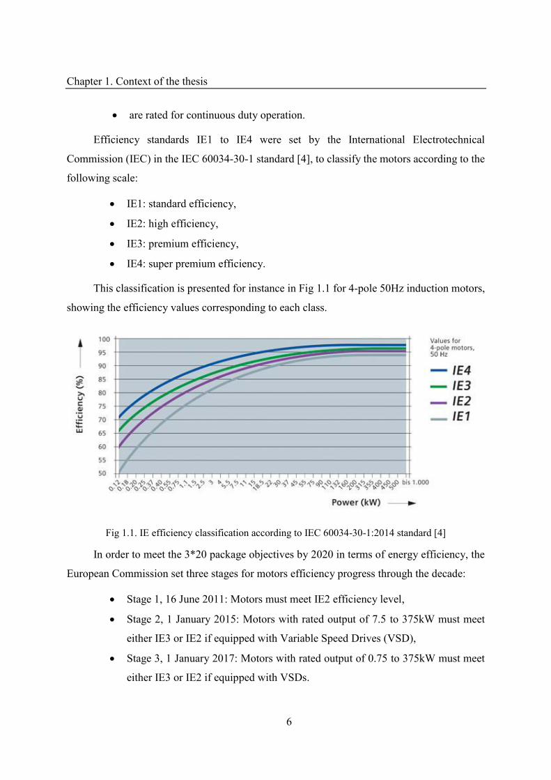
This classification is presented for instance in Fig 1.1 for 4-pole 50Hz induction motors,
showing the efficiency values corresponding to each class.
Fig 1.1. IE efficiency classification according to IEC 60034-30-1:2014 standard [4]
In order to meet the 3*20 package objectives by 2020 in terms of energy efficiency, the
European Commission set three stages for motors efficiency progress through the decade:
• Stage 1, 16 June 2011: Motors must meet IE2 efficiency level,
• Stage 2, 1 January 2015: Motors with rated output of 7.5 to 375kW must meet
either IE3 or IE2 if equipped with Variable Speed Drives (VSD),
• Stage 3, 1 January 2017: Motors with rated output of 0.75 to 375kW must meet
either IE3 or IE2 if equipped with VSDs.
Chapter 1. Context of the thesis
7
The IE4 efficiency standard shown in Fig 1.1 is not part of the actual scopes of the
commission program but is defined for future stages. The proposed stages and standards are
respected by the motors and drives manufacturers, in addition to the researches and projects
which are initiated to study the performance of high-efficient motors [5], and to improve the
energy efficiency to meet the 3*20 package for 2020 and its extension to 2030.
Calculations and results obtained in this thesis are based on an IE2 high-efficiency IM,
then compared with the results obtained by an IE3 premium-efficiency IM, to show the effect
of the proposed method on the energy efficiency, according to the motor standard. Hence, a
first step for carrying a study on the IM is by defining an accurate mathematical model, which
predicts the motor performance according to the required operating conditions.
1.2 State of Art of Existing Induction Motors Models
An essential part of the studies on electric motors is based on their modeling, which must
be as similar as possible to the real motor performance, in order to predict the outcomes of any
application or control. In the case of squirrel-cage induction motors, several types of models
are developed in literature based on different assumptions and used according to the operating
conditions (transient or steady state).
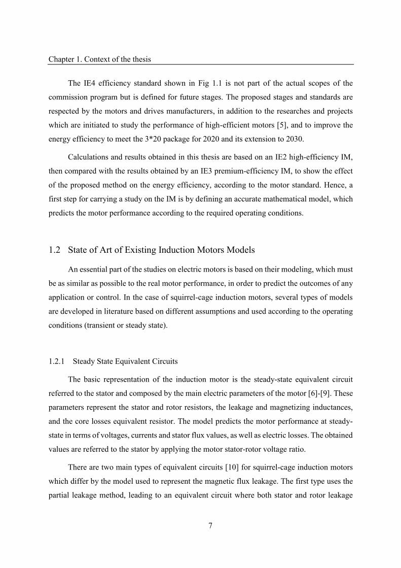
1.2.1 Steady State Equivalent Circuits
The basic representation of the induction motor is the steady-state equivalent circuit
referred to the stator and composed by the main electric parameters of the motor [6]-[9]. These
parameters represent the stator and rotor resistors, the leakage and magnetizing inductances,
and the core losses equivalent resistor. The model predicts the motor performance at steady-
state in terms of voltages, currents and stator flux values, as well as electric losses. The obtained
values are referred to the stator by applying the motor stator-rotor voltage ratio.
There are two main types of equivalent circuits [10] for squirrel-cage induction motors
which differ by the model used to represent the magnetic flux leakage. The first type uses the
partial leakage method, leading to an equivalent circuit where both stator and rotor leakage
Chapter 1. Context of the thesis
8
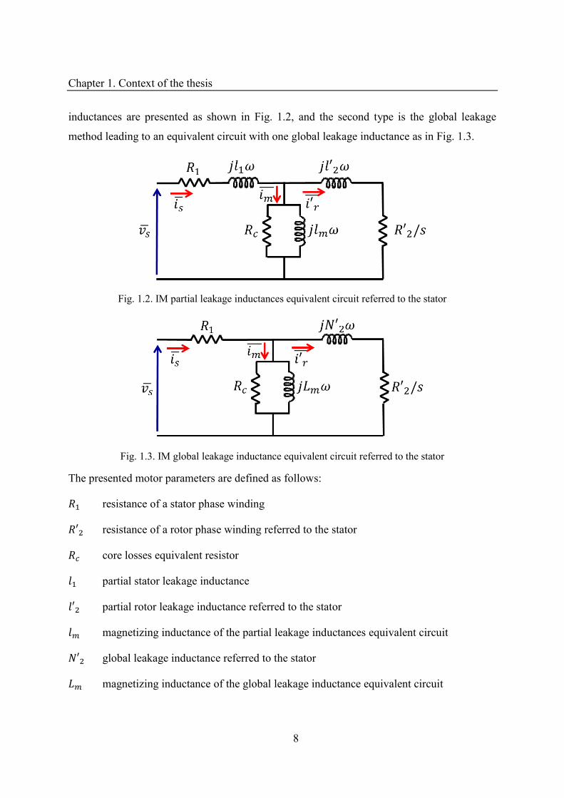
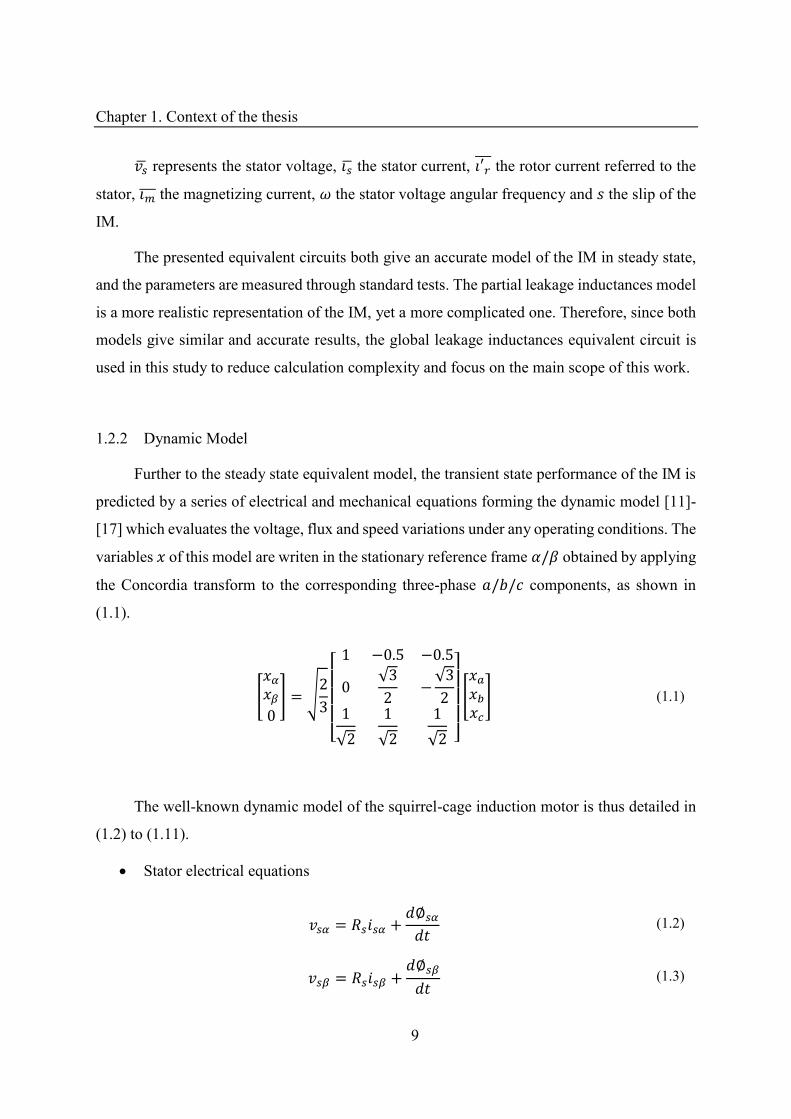
inductances are presented as shown in Fig. 1.2, and the second type is the global leakage
method leading to an equivalent circuit with one global leakage inductance as in Fig. 1.3.
Fig. 1.2. IM partial leakage inductances equivalent circuit referred to the stator
Fig. 1.3. IM global leakage inductance equivalent circuit referred to the stator
The presented motor parameters are defined as follows:
resistance of a stator phase winding ′ resistance of a rotor phase winding referred to the stator
core losses equivalent resistor
partial stator leakage inductance ′ partial rotor leakage inductance referred to the stator
magnetizing inductance of the partial leakage inductances equivalent circuit ′ global leakage inductance referred to the stator
magnetizing inductance of the global leakage inductance equivalent circuit
Chapter 1. Context of the thesis
9
represents the stator voltage, � the stator current, �′ the rotor current referred to the
stator, � the magnetizing current, � the stator voltage angular frequency and the slip of the
IM.
The presented equivalent circuits both give an accurate model of the IM in steady state,
and the parameters are measured through standard tests. The partial leakage inductances model
is a more realistic representation of the IM, yet a more complicated one. Therefore, since both
models give similar and accurate results, the global leakage inductances equivalent circuit is
used in this study to reduce calculation complexity and focus on the main scope of this work.
1.2.2 Dynamic Model
Further to the steady state equivalent model, the transient state performance of the IM is
predicted by a series of electrical and mechanical equations forming the dynamic model [11]-
[17] which evaluates the voltage, flux and speed variations under any operating conditions. The
variables of this model are writen in the stationary reference frame / obtained by applying
the Concordia transform to the corresponding three-phase / / components, as shown in
(1.1).
[ ] = √ [ − . − .√ −√√ √ √ ]
[ ] (1.1)
The well-known dynamic model of the squirrel-cage induction motor is thus detailed in
(1.2) to (1.11).
• Stator electrical equations
= + ∅ (1.2)
= + ∅ (1.3)
Chapter 1. Context of the thesis
10
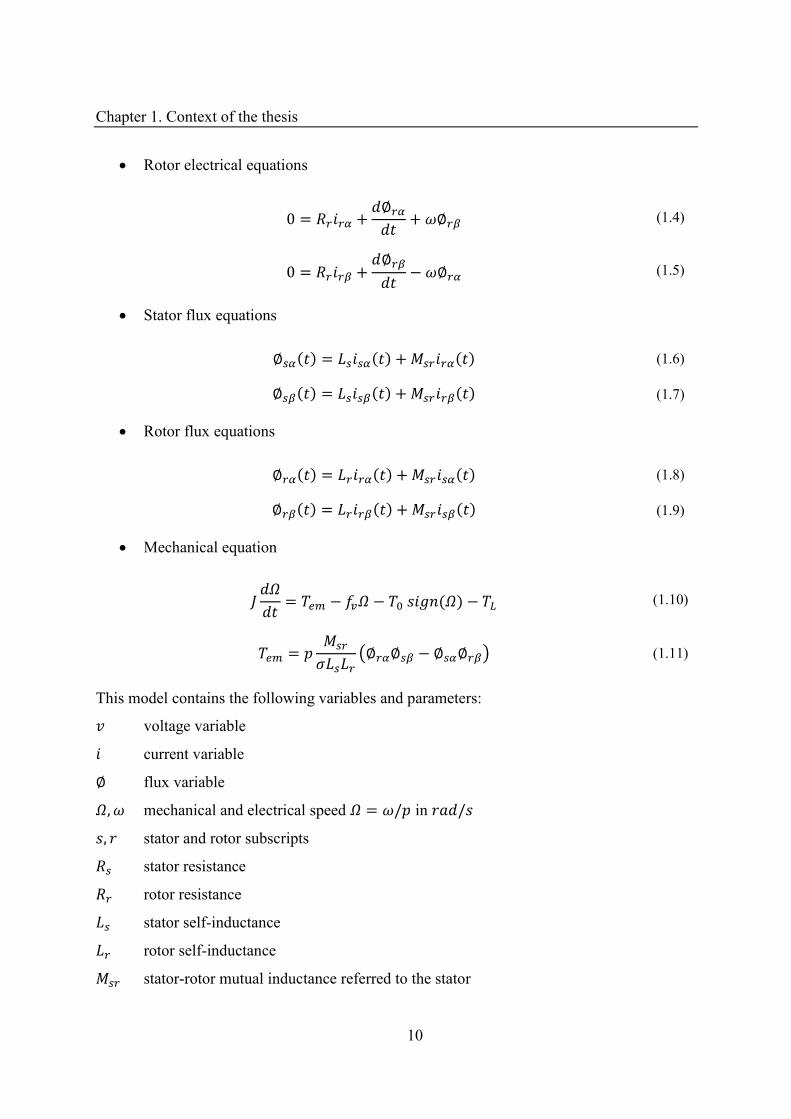
• Rotor electrical equations
= + ∅ + �∅ (1.4)
= + ∅ − �∅ (1.5)
• Stator flux equations ∅ = + (1.6) ∅ = + (1.7)
• Rotor flux equations ∅ = + (1.8) ∅ = + (1.9)
• Mechanical equation � = − �� − � − (1.10)
= � (∅ ∅ − ∅ ∅ ) (1.11)
This model contains the following variables and parameters:
voltage variable
current variable ∅ flux variable �,� mechanical and electrical speed � = �/ in / , stator and rotor subscripts
stator resistance
rotor resistance
stator self-inductance
rotor self-inductance
stator-rotor mutual inductance referred to the stator
Chapter 1. Context of the thesis
11
� motor dispersion coefficient � = − 2
number of pole pairs of the motor
total motor load inertia � viscous friction coefficient
dry friction torque em electromagnetic torque L load torque
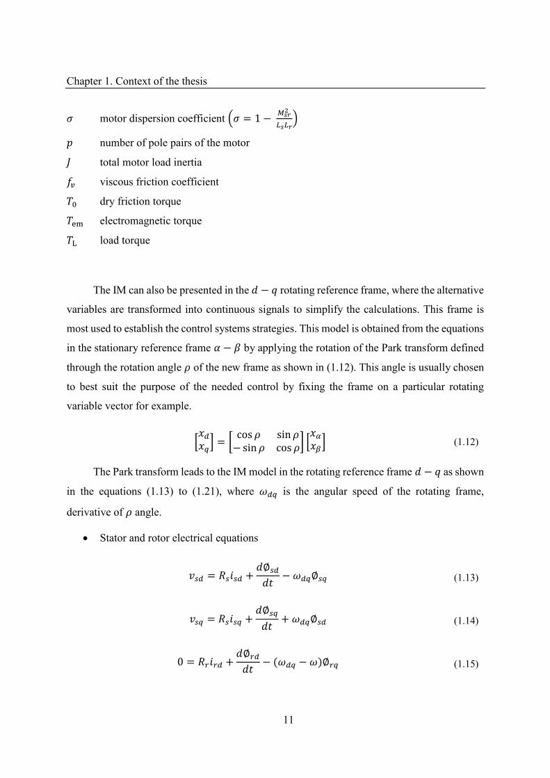
The IM can also be presented in the − rotating reference frame, where the alternative
variables are transformed into continuous signals to simplify the calculations. This frame is
most used to establish the control systems strategies. This model is obtained from the equations
in the stationary reference frame − by applying the rotation of the Park transform defined
through the rotation angle � of the new frame as shown in (1.12). This angle is usually chosen
to best suit the purpose of the needed control by fixing the frame on a particular rotating
variable vector for example.
[ ] = [ cos � sin �− sin � cos �] [ ] (1.12)
The Park transform leads to the IM model in the rotating reference frame − as shown
in the equations (1.13) to (1.21), where � is the angular speed of the rotating frame,
derivative of � angle.
• Stator and rotor electrical equations
= + ∅ − � ∅ (1.13)
= + ∅ + � ∅ (1.14)
= + ∅ − � − � ∅ (1.15)
Chapter 1. Context of the thesis
12
= + ∅ + (� −�)∅ (1.16)
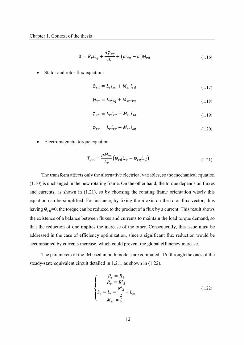
• Stator and rotor flux equations ∅ = + (1.17) ∅ = + (1.18) ∅ = + (1.19) ∅ = + (1.20)
• Electromagnetic torque equation
= (∅ − ∅ ) (1.21)
The transform affects only the alternative electrical variables, so the mechanical equation
(1.10) is unchanged in the new rotating frame. On the other hand, the torque depends on fluxes
and currents, as shown in (1.21), so by choosing the rotating frame orientation wisely this
equation can be simplified. For instance, by fixing the -axis on the rotor flux vector, thus
having ∅ =0, the torque can be reduced to the product of a flux by a current. This result shows
the existence of a balance between fluxes and currents to maintain the load torque demand, so
that the reduction of one implies the increase of the other. Consequently, this issue must be
addressed in the case of efficiency optimization, since a significant flux reduction would be
accompanied by currents increase, which could prevent the global efficiency increase.
The parameters of the IM used in both models are computed [16] through the ones of the
steady-state equivalent circuit detailed in 1.2.1, as shown in (1.22).
{ == ′= = ′ += (1.22)
Chapter 1. Context of the thesis
13
This model is widely used in literature of IM researches. It represents the IM performance
in different conditions and takes into consideration the effect of the Joule and mechanical
losses. However, studies are carried to establish more accurate dynamic models which take into
account imperfections of the motor and magnetic losses.
1.2.3 Improved Dynamic Models
The improvement of the IM model accuracy is the scope of many studies in order to
predict its performance in unusual cases and to include all possible losses. For instance, some
proposed models include the magnetic saturation effect as in [18] and [19] by representing
inductances as functions of the flux and the magnetic structure of the motor, others include the
temperature and skin effect as in [20] and [21].
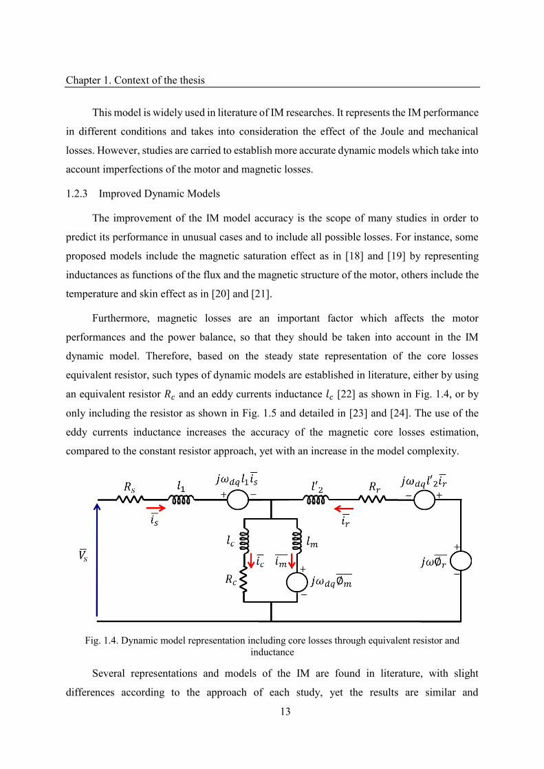
Furthermore, magnetic losses are an important factor which affects the motor
performances and the power balance, so that they should be taken into account in the IM
dynamic model. Therefore, based on the steady state representation of the core losses
equivalent resistor, such types of dynamic models are established in literature, either by using
an equivalent resistor and an eddy currents inductance [22] as shown in Fig. 1.4, or by
only including the resistor as shown in Fig. 1.5 and detailed in [23] and [24]. The use of the
eddy currents inductance increases the accuracy of the magnetic core losses estimation,
compared to the constant resistor approach, yet with an increase in the model complexity.
Fig. 1.4. Dynamic model representation including core losses through equivalent resistor and inductance
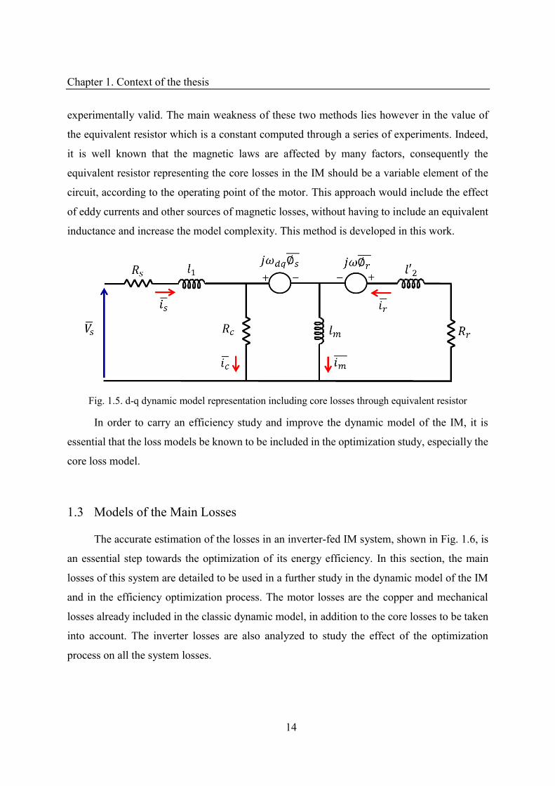
Several representations and models of the IM are found in literature, with slight
differences according to the approach of each study, yet the results are similar and
Chapter 1. Context of the thesis
14
experimentally valid. The main weakness of these two methods lies however in the value of
the equivalent resistor which is a constant computed through a series of experiments. Indeed,
it is well known that the magnetic laws are affected by many factors, consequently the
equivalent resistor representing the core losses in the IM should be a variable element of the
circuit, according to the operating point of the motor. This approach would include the effect
of eddy currents and other sources of magnetic losses, without having to include an equivalent
inductance and increase the model complexity. This method is developed in this work.
Fig. 1.5. d-q dynamic model representation including core losses through equivalent resistor
In order to carry an efficiency study and improve the dynamic model of the IM, it is
essential that the loss models be known to be included in the optimization study, especially the
core loss model.
1.3 Models of the Main Losses
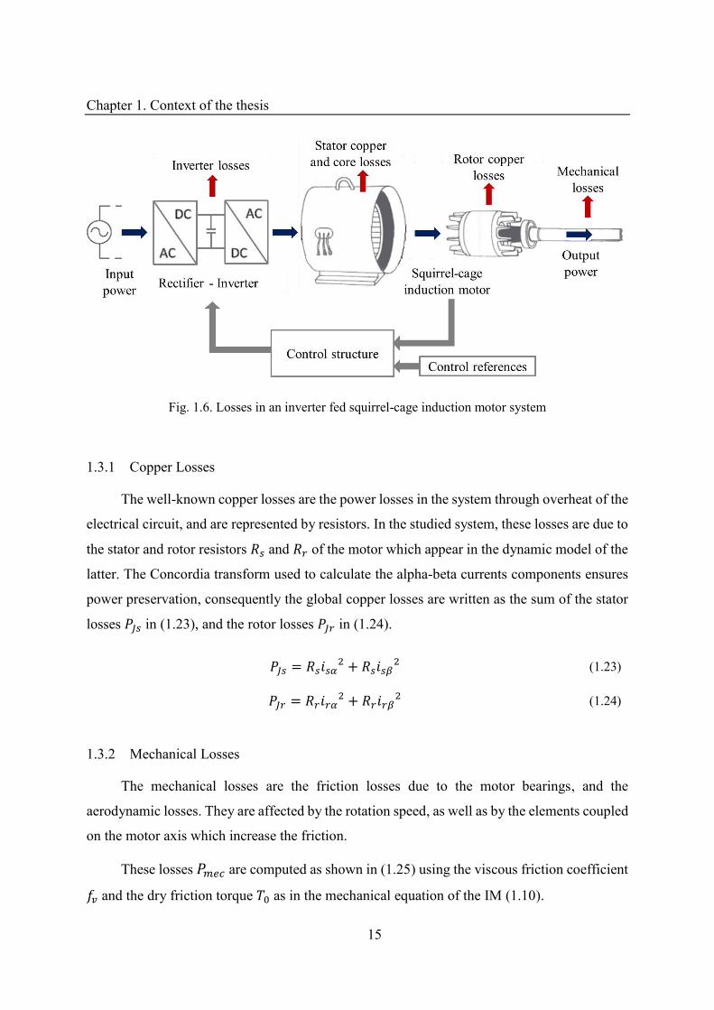
The accurate estimation of the losses in an inverter-fed IM system, shown in Fig. 1.6, is
an essential step towards the optimization of its energy efficiency. In this section, the main
losses of this system are detailed to be used in a further study in the dynamic model of the IM
and in the efficiency optimization process. The motor losses are the copper and mechanical
losses already included in the classic dynamic model, in addition to the core losses to be taken
into account. The inverter losses are also analyzed to study the effect of the optimization
process on all the system losses.
Chapter 1. Context of the thesis
15
Fig. 1.6. Losses in an inverter fed squirrel-cage induction motor system
1.3.1 Copper Losses
The well-known copper losses are the power losses in the system through overheat of the
electrical circuit, and are represented by resistors. In the studied system, these losses are due to
the stator and rotor resistors and of the motor which appear in the dynamic model of the
latter. The Concordia transform used to calculate the alpha-beta currents components ensures
power preservation, consequently the global copper losses are written as the sum of the stator
losses � in (1.23), and the rotor losses � in (1.24).
� = + (1.23)
� = + (1.24)
1.3.2 Mechanical Losses
The mechanical losses are the friction losses due to the motor bearings, and the
aerodynamic losses. They are affected by the rotation speed, as well as by the elements coupled
on the motor axis which increase the friction.
These losses are computed as shown in (1.25) using the viscous friction coefficient
� and the dry friction torque as in the mechanical equation of the IM (1.10).
Chapter 1. Context of the thesis
16
= �� + � � = �� + |�| (1.25)
1.3.3 Core Losses
The estimation of core losses is an important research domain because of the complexity
of magnetic laws and the sensibility of the magnetic circuits to the operating conditions and to
the type of material [25]. Thus, they are evaluated in many studies by simply deducting the
other known losses and output power, from the input power. In other cases, they are represented
by an equivalent resistor in the circuit, and the losses values are computed using the current in
this resistor, similarly to the copper losses [58]. Some authors went further by using more
specific models, defining these losses as functions of the frequency , and the magnetic field
[26]-[55] or flux ∅ [18], as shown in (1.26) and (1.27), where , and are specific
coefficients computed through tests. = (1.26) = ∅ + ∅ (1.27)
In a more accurate approach, core losses are estimated, according to the Bertotti law [27]-
[29], as the sum of the magnetic losses due to the hysteresis effect �, the Eddy currents effect
and the excess losses � caused by the imperfections inside the magnetic circuit. These
losses are written [30] as functions of the maximum value of the magnetic field � and the
voltage frequency as shown in (1.28).
= � + + � = ′� � + ′ � + ′ � �.5 .5 (1.28)
This model contains similarities with the previously presented models, yet in a more
detailed and precise approach considering the magnetic characteristics of the analyzed circuit.
This model is used in the present study for core losses computation.
The coefficients of the three magnetic losses ′�, ′ and ′ � are not provided by the
motor constructor, their values are measured through a series of experiments [31]. Furthermore,
the presented model is only valid for sinusoidal-fed magnetic circuits, and in the inverter-fed
case, the effect of the magnetic field harmonics should be taken into account [32]. Thus, as
detailed in [33]-[36], the model becomes as shown in (1.29).
Chapter 1. Context of the thesis
17
= ′� � + ′ ∫| | + ′ � .5∫| | .5 (1.29)
Authors have established some simpler versions of the core losses model for non-
sinusoidal cases without altering the results [37]. Indeed, by applying the Fourier series, the
model becomes as shown in (1.30), where represents the harmonic rank [38].
= ′� � + ′ ∑ �� + ′ � .5∑ .5 �.5� (1.30)
The core losses model is slightly complicated to use but gives accurate results in
sinusoidal and inverter-fed systems while taking into consideration the effect of the geometry
of the magnetic structure through the coefficients, as well as the effect of the magnetic field
and the frequency.
In order to use the core loss model with measurable variables, the magnetic field is
replaced by the product of the flux / and a coefficient characteristic of the magnetic
circuit. For instance, equation (1.28) becomes as in (1.31) with the new core loss coefficients �, and �, products of ′�, ′ and ′ � by . Similarly, equation (1.30) becomes as in
(1.32).
= � � + � + � �.5 (1.31)
= � � + ∑ � � + � ∑ .5 �.5
� (1.32)
These losses are a main point in this study, since as mentioned in 1.2, they must be taken
into account in the dynamic model of the IM using an accurate loss model, considering the
effect of the magnetic field and the frequency, which is ensured by the Bertotti model.
1.3.4 Inverter Losses
In the inverter-motor system, in addition to the motor losses, it is essential to evaluate
the losses inside the inverter which are mainly affected by the currents flowing through the
phases and switches. These losses are divided into two main parts: the conduction losses caused

Chapter 1. Context of the thesis
18
by the voltage drop in the switches at on-state, and the switching losses due to the switching
delay of the elements.
The computation of these losses is not an easy task because of the high switching
frequency. In general, the losses at steady-state are averaged over one or multiple switching
periods. However, in the case of online calculations or simulations as presented in [39] and
[40], and in order to increase accuracy, the conduction losses are instantaneously computed
according to the on/off state of the elements, and the switching losses are averaged over a
switching period.
1.3.4.1 Conduction Losses
An inverter leg is formed by two switches in series, each one in parallel with an inverted
diode. Both switches work in opposite states to avoid short-circuiting the voltage source, and
the diodes states are imposed by the sign of the current. The conduction losses depend on the
passing element, so it is essential to identify the latter at each state. A series of switching
functions is therefore defined to calculate the voltage drop in the switches:
• The function defines the state of the first switch in the studied inverter leg. It is equal
to zero for off-state, which corresponds to the on-state of the second switch of the same
leg, and to 1 for the on-state,
• The function = − takes the values 1 for on and -1 for off-state,
• The function = + � � . which values vary with the sign of the motor stator
current flowing through the switches, in order to identify the element in passing state.
The voltage drops according to the state of the switches and to the sign of the flowing
current are shown in Table 1.1, where � represents the passing state voltage drop of a
switch, and the passing state voltage drop of a diode.
Table 1.1. Conduction voltage drops per inverter leg
= = − � > � � < − − �
Chapter 1. Context of the thesis
19
The conduction voltage drop shown in Table 1.1 in each inverter leg is also given
by an analytical equation, according to the state of the switches, and the sign of the current, as
shown in (1.33). = . [ � + − ] (1.33)
The voltage drop values � and of the elements are obtained by the linear equations
(1.34) based on the switches zero-current voltage drop � and and passing resistors �
and given by the manufacturer.
{ � = � + �= + (1.34)
Consequently, the inverter conduction losses can be written as in (1.35), where varies
according to the state of the switch and the sign of the current as described earlier. Thus, by
integrating the loss model over a switching period, would be equal to the duty cycle if the
current was positive, and equal to − otherwise. The integrated conduction model is
therefore obtained as shown in (1.36). = | |. [ � + � + − + ] (1.35)
{ > : = . [ � + � + − + ] < : = − . [ − � + � + + ] (1.36)
1.3.4.2 Switching Losses
Since the commutations of the switches happen at constant frequency, their losses are
averaged [41]-[42]. Indeed, 4 commutations occur in each inverter leg over a switching period,
and the on/off delays are provided by the manufacturer. Through these delays, the voltage in
the switches is averaged to half the DC bus voltage , and then the switching losses voltage
drop is computed as in (1.37), and the conduction losses as in (1.38).
= × ( + ) = ( + ) (1.37)
Chapter 1. Context of the thesis
20
= ( + ) | | (1.38)
Based on the above, the global inverter voltage drop can be computed through (1.33) and
(1.37), and the global inverter losses in each leg through (1.36) and (1.38). These losses vary
with the currents, but depend much on the switches structure because of the passing resistors
and switching delays. Generally, silicon-based (Si) IGBT are used, but recently, new Silicon-
Carbide (SiC) structures are being manufactured, and ensure better performances in terms of
higher switching frequencies, high temperature operation, and most importantly, average
reductions of 40% power loss compared to the Si structures. These reductions are due to their
smaller semi-conductor structure leading to reduced passing resistors and the capacity to
increase the switching frequency and reduce the switching delays.
1.3.5 Summary
To sum up, the main losses in the inverter-fed IM system are the copper, core and
mechanical losses in the motor, in addition to the inverter losses. They vary according to the
operating point and power requirements, and can have significant values compared to the input
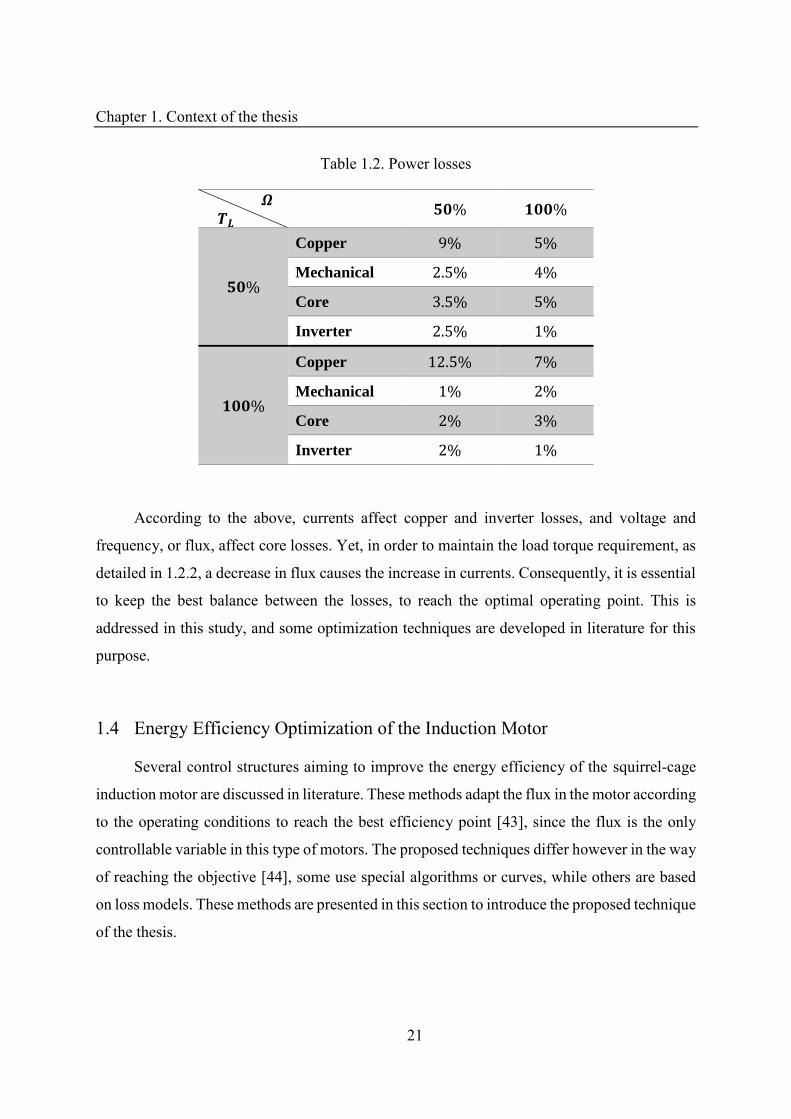
power. Table 1.2 presents results on a 5.5kW IE2 IM, showing percentages of the main losses
compared to the system input power at different operating points in the torque-speed plane.
Values show that copper losses are the most important ones, and that core losses are also
significant, especially at low torque.
It should be noted that the losses depend on different operating variables, so that any
optimization process should preserve a balance between them, since the decrease of some
variables would increase others. Indeed, the described losses are dependent as follow:
• Copper losses depend on the currents,
• Mechanical losses depend on the speed,
• Core losses depend on the voltage and frequency,
• Inverter losses depend on the currents, DC voltage and switching frequency.
Chapter 1. Context of the thesis
21
Table 1.2. Power losses � �� % %
%
Copper % %
Mechanical . % %
Core . % %
Inverter . % %
%
Copper . % %
Mechanical % %
Core % %
Inverter % %
According to the above, currents affect copper and inverter losses, and voltage and
frequency, or flux, affect core losses. Yet, in order to maintain the load torque requirement, as
detailed in 1.2.2, a decrease in flux causes the increase in currents. Consequently, it is essential
to keep the best balance between the losses, to reach the optimal operating point. This is
addressed in this study, and some optimization techniques are developed in literature for this
purpose.
1.4 Energy Efficiency Optimization of the Induction Motor
Several control structures aiming to improve the energy efficiency of the squirrel-cage
induction motor are discussed in literature. These methods adapt the flux in the motor according
to the operating conditions to reach the best efficiency point [43], since the flux is the only
controllable variable in this type of motors. The proposed techniques differ however in the way
of reaching the objective [44], some use special algorithms or curves, while others are based
on loss models. These methods are presented in this section to introduce the proposed technique
of the thesis.
Chapter 1. Context of the thesis
22
1.4.1 Search Control
The Search Control (SC) is an efficiency optimization technique which tracks the lowest
possible input power of the motor for each operating point. The input power value is
continuously measured and compared to its previous state. The algorithm then decides, whether
to keep on varying the flux like its previous state if the input power decreases, or in the other
way if the power increases [45]-[47]. By doing so, the system converges to the best efficiency
point which corresponds to the minimal input power while keeping on the same output power
of the motor. However, an average delay of one second is introduced by each
increment/decrement of flux in the basic SC, which causes a global delay of 15 to 20 seconds
to reach the optimal operating point. In addition, the control will keep on oscillating around the
optimal flux value when in steady state, causing instability of the whole electrical and
mechanical system.
Therefore, some other versions of the basic SC are established in literature aiming to
improve its performance and reduce the delays to reach the steady-state. For instance, the
‘Golden section’ technique [48] is proposed in literature. It varies the flux increment on the
basis of these golden sections theory, in order to find the best efficiency point in a reduced
delay. Similarly, artificial intelligence is used in several works [49]-[53] to enhance the search
process through training a fuzzy logic controller according to power v/s flux or efficiency v/s
flux curves, in order to reach the optimal operating point with reduced delays. Fig. 1.7 shows
an example of the improvement in optimal flux tracking between the basic SC and the one with
an intelligent controller simulated under MATLAB/Simulink. Delays are clearly reduced, as
well as oscillations at steady state. Simulations and experimental tests on the SC techniques
validate the improvement in motor efficiency and the decrease in the motor losses.
The advantage of these search control techniques is that they are independent of the
motor type or rated power, and do not require any previous knowledge of the system
parameters. However, the above detailed problems yet remain significant in terms of delays
and oscillations, even if reduced by the enhancement techniques proposed, which could cause
the algorithm divergence in cases of rapid load variation or amplified noise in the measured
signals.
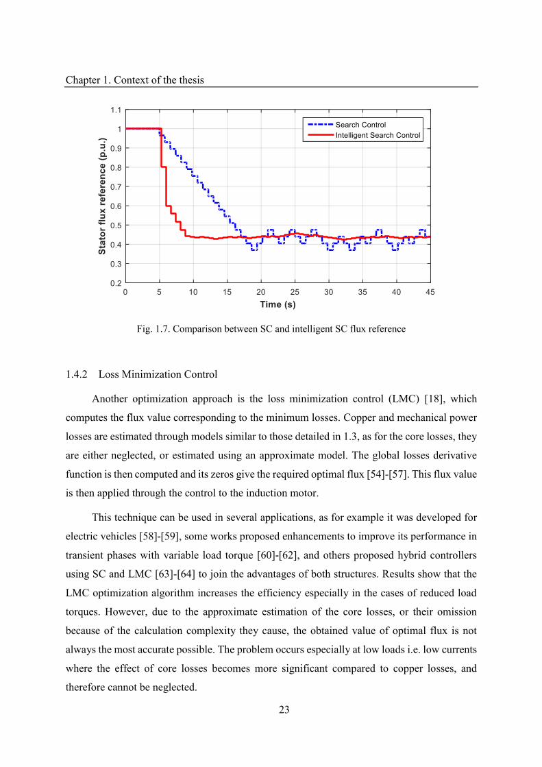
Chapter 1. Context of the thesis
23
Fig. 1.7. Comparison between SC and intelligent SC flux reference
1.4.2 Loss Minimization Control
Another optimization approach is the loss minimization control (LMC) [18], which
computes the flux value corresponding to the minimum losses. Copper and mechanical power
losses are estimated through models similar to those detailed in 1.3, as for the core losses, they
are either neglected, or estimated using an approximate model. The global losses derivative
function is then computed and its zeros give the required optimal flux [54]-[57]. This flux value
is then applied through the control to the induction motor.
This technique can be used in several applications, as for example it was developed for
electric vehicles [58]-[59], some works proposed enhancements to improve its performance in
transient phases with variable load torque [60]-[62], and others proposed hybrid controllers
using SC and LMC [63]-[64] to join the advantages of both structures. Results show that the
LMC optimization algorithm increases the efficiency especially in the cases of reduced load
torques. However, due to the approximate estimation of the core losses, or their omission
because of the calculation complexity they cause, the obtained value of optimal flux is not
always the most accurate possible. The problem occurs especially at low loads i.e. low currents
where the effect of core losses becomes more significant compared to copper losses, and
therefore cannot be neglected.
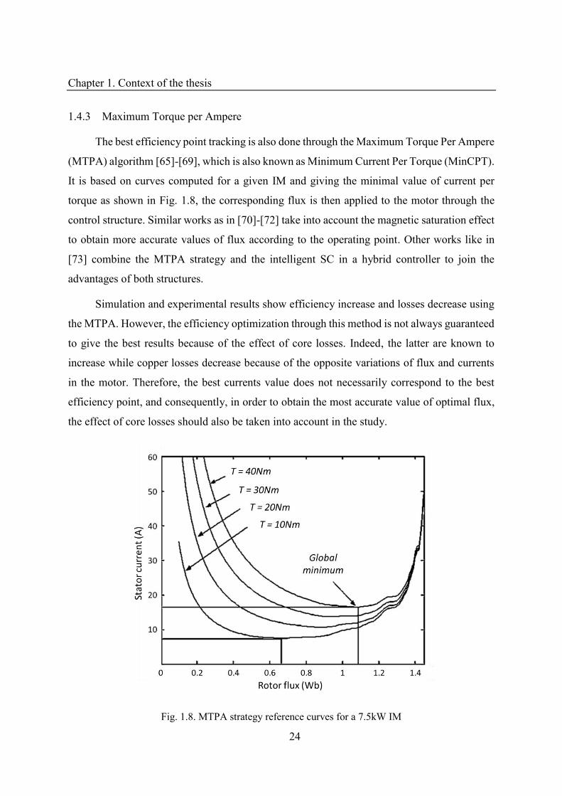
Chapter 1. Context of the thesis
24
1.4.3 Maximum Torque per Ampere
The best efficiency point tracking is also done through the Maximum Torque Per Ampere
(MTPA) algorithm [65]-[69], which is also known as Minimum Current Per Torque (MinCPT).
It is based on curves computed for a given IM and giving the minimal value of current per
torque as shown in Fig. 1.8, the corresponding flux is then applied to the motor through the
control structure. Similar works as in [70]-[72] take into account the magnetic saturation effect
to obtain more accurate values of flux according to the operating point. Other works like in
[73] combine the MTPA strategy and the intelligent SC in a hybrid controller to join the
advantages of both structures.
Simulation and experimental results show efficiency increase and losses decrease using
the MTPA. However, the efficiency optimization through this method is not always guaranteed
to give the best results because of the effect of core losses. Indeed, the latter are known to
increase while copper losses decrease because of the opposite variations of flux and currents
in the motor. Therefore, the best currents value does not necessarily correspond to the best
efficiency point, and consequently, in order to obtain the most accurate value of optimal flux,
the effect of core losses should also be taken into account in the study.
Fig. 1.8. MTPA strategy reference curves for a 7.5kW IM

Chapter 1. Context of the thesis
25
1.4.4 Summary
The improvement methods found in literature are proven to optimize the energy
efficiency of induction motors and reduce their losses. Yet, each one of the methods has
weaknesses either in terms of dynamic response in the case of SC, or in terms of optimal
efficiency accuracy in the case of LMC and MTPA. Core losses constitute an important aspect
of efficiency estimation; therefore, it cannot be omitted or taken into consideration through an
approximate approach.
The proposed method in this study tracks the best efficiency point avoiding the dynamic
delays and oscillations, and taking the core losses into consideration the most accurately
possible. The technique is based on off-line measurements to accurately map the optimal
reference flux in the torque-speed plane. The approach is systematic and can be declined very
quickly on any asynchronous machine.
Conclusion
This work is well positioned in the heart of the European Commission sustainability
project, by contributing in the efficiency optimization objective. For this purpose, models of
the squirrel-cage induction motor were presented in this chapter, as well as loss models aiming
to analyze the optimization effect on the main losses in the IM and in the inverter. Hence,
several techniques found in the literature serving that goal are presented. However, these
methods lack accuracy in some cases and can be subject to dynamic instabilities.
Through the present study, an improved optimization method is proposed, avoiding the
problems of the existing techniques, and based on an improved dynamic model of the induction
motor which is to be presented in the next chapter. This model takes into account the effect of
the core losses, in addition to the other motor losses which are included in the classic model
version. The goal is to find the flux corresponding to the optimal balance between the system
losses, and include it into the control structures afterward.
Chapter 2 Induction Motor Model Taking Core Losses into
Account
Table of Contents Introduction ................................................................................................................ 27
2.1 Model Parameters Measurement .................................................................... 27
2.1.1 Mechanical Parameters ............................................................................... 27
2.1.2 Electrical Parameters .................................................................................. 28
2.1.3 Core Losses Model Coefficients ................................................................. 30
2.2 Including Core Losses in the IM Model ........................................................ 31
2.2.1 Equivalent Torque Approach...................................................................... 32
2.2.2 Equivalent Resistor Approach .................................................................... 32
2.2.3 Summary and Analysis ............................................................................... 34
2.3 Including Variable Core Losses ..................................................................... 37
2.3.1 Enhancement of the Improved Dynamic Model ......................................... 38
2.3.2 Simulation Results and Experimental Validation ....................................... 38
Conclusion .................................................................................................................. 39
Chapter 2. Induction Motor Model Taking Core Losses into Account
27
Introduction
Establishing an accurate mathematical model is an essential step for any study to be
carried on a motor, as it allows a precise simulation of the performance to be expected under
specific conditions. The classic model of an IM lacks accuracy because it neglects the effect of
core losses.
In this chapter, an improved model taking into account such losses is thus proposed. This
model is based on the addition of a variable resistor representing core losses which depend on
the magnetic field and frequency. It is calculated using the Bertotti model presented in 1.3.3.
In addition, the experimental measurement and identification of motor parameters are detailed,
especially for the core losses parameters to be used in the proposed model. The variation of
these losses with the operating conditions is also taken into account.
2.1 Model Parameters Measurement
The studied motor is a 5.5kW Leroy-Somer squirrel-cage induction motor LSES 132 SU
compliant with IE2 efficiency standard. The parameters of the studied motor are computed
through a series of experiments carried in several operating conditions. The obtained
parameters define the classic dynamic model of the IM detailed in 1.2.2, as well as the core
losses model presented in 1.3.3.
2.1.1 Mechanical Parameters
The mechanical parameters of the IM that need to be measured are the viscous friction
coefficient � and the dry friction torque that define the friction losses on the axe of the
motor, and take part in the mechanical equation of the IM dynamic model. They are computed
through a zero-load deceleration experiment, where the IM initially rotating slightly below the
base speed is powered off. The speed is measured and is presented in Fig. 2.1.
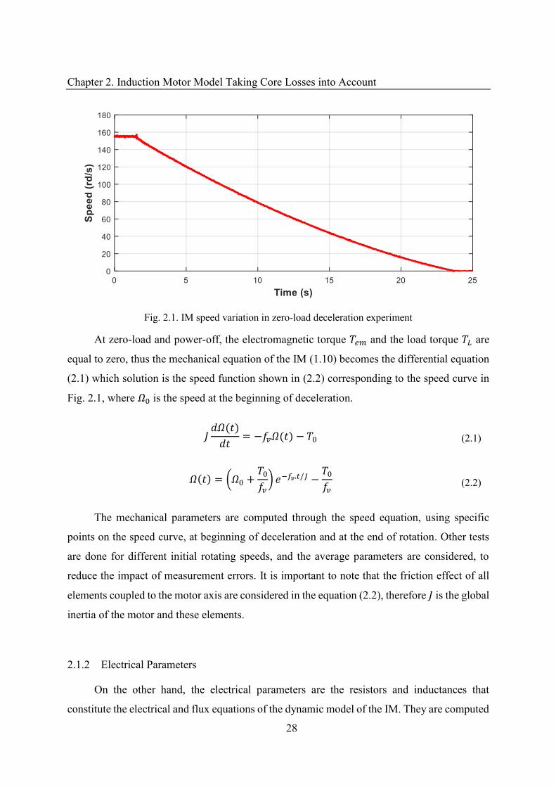
Chapter 2. Induction Motor Model Taking Core Losses into Account
28
Fig. 2.1. IM speed variation in zero-load deceleration experiment
At zero-load and power-off, the electromagnetic torque and the load torque are
equal to zero, thus the mechanical equation of the IM (1.10) becomes the differential equation
(2.1) which solution is the speed function shown in (2.2) corresponding to the speed curve in
Fig. 2.1, where � is the speed at the beginning of deceleration. � = − �� − (2.1)
� = (� + �) − �. /� − � (2.2)
The mechanical parameters are computed through the speed equation, using specific
points on the speed curve, at beginning of deceleration and at the end of rotation. Other tests
are done for different initial rotating speeds, and the average parameters are considered, to
reduce the impact of measurement errors. It is important to note that the friction effect of all
elements coupled to the motor axis are considered in the equation (2.2), therefore is the global
inertia of the motor and these elements.
2.1.2 Electrical Parameters
On the other hand, the electrical parameters are the resistors and inductances that
constitute the electrical and flux equations of the dynamic model of the IM. They are computed
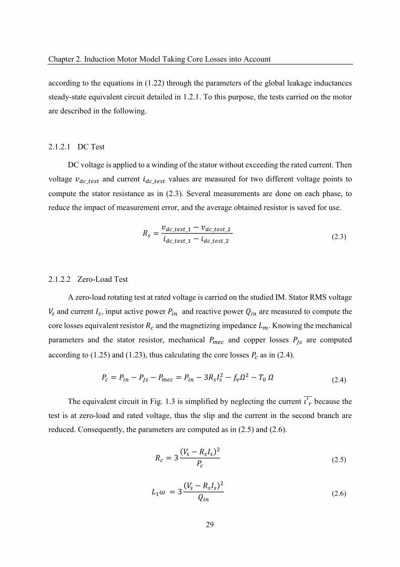
Chapter 2. Induction Motor Model Taking Core Losses into Account
29
according to the equations in (1.22) through the parameters of the global leakage inductances
steady-state equivalent circuit detailed in 1.2.1. To this purpose, the tests carried on the motor
are described in the following.
2.1.2.1 DC Test
DC voltage is applied to a winding of the stator without exceeding the rated current. Then
voltage _ and current _ values are measured for two different voltage points to
compute the stator resistance as in (2.3). Several measurements are done on each phase, to
reduce the impact of measurement error, and the average obtained resistor is saved for use.
= _ _ − _ _ _ _ − _ _ (2.3)
2.1.2.2 Zero-Load Test
A zero-load rotating test at rated voltage is carried on the studied IM. Stator RMS voltage
and current , input active power � and reactive power � are measured to compute the
core losses equivalent resistor and the magnetizing impedance . Knowing the mechanical
parameters and the stator resistor, mechanical and copper losses � are computed
according to (1.25) and (1.23), thus calculating the core losses as in (2.4). = � − � − = � − − �� − � (2.4)
The equivalent circuit in Fig. 1.3 is simplified by neglecting the current �′ because the
test is at zero-load and rated voltage, thus the slip and the current in the second branch are
reduced. Consequently, the parameters are computed as in (2.5) and (2.6).
= − (2.5)
� = − � (2.6)
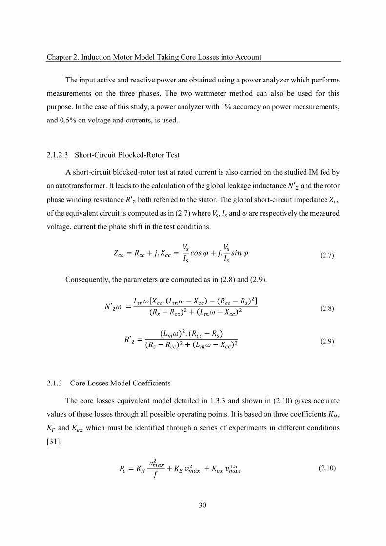
Chapter 2. Induction Motor Model Taking Core Losses into Account
30
The input active and reactive power are obtained using a power analyzer which performs
measurements on the three phases. The two-wattmeter method can also be used for this
purpose. In the case of this study, a power analyzer with 1% accuracy on power measurements,
and 0.5% on voltage and currents, is used.
2.1.2.3 Short-Circuit Blocked-Rotor Test
A short-circuit blocked-rotor test at rated current is also carried on the studied IM fed by
an autotransformer. It leads to the calculation of the global leakage inductance ′ and the rotor
phase winding resistance ′ both referred to the stator. The global short-circuit impedance
of the equivalent circuit is computed as in (2.7) where , and � are respectively the measured
voltage, current the phase shift in the test conditions.
= + . = � + . � (2.7)
Consequently, the parameters are computed as in (2.8) and (2.9).
′ � = �[ . � − − − ]− + � − (2.8)
′ = � . −− + � − (2.9)
2.1.3 Core Losses Model Coefficients
The core losses equivalent model detailed in 1.3.3 and shown in (2.10) gives accurate
values of these losses through all possible operating points. It is based on three coefficients �,
and � which must be identified through a series of experiments in different conditions
[31].
= � � + � + � �.5 (2.10)
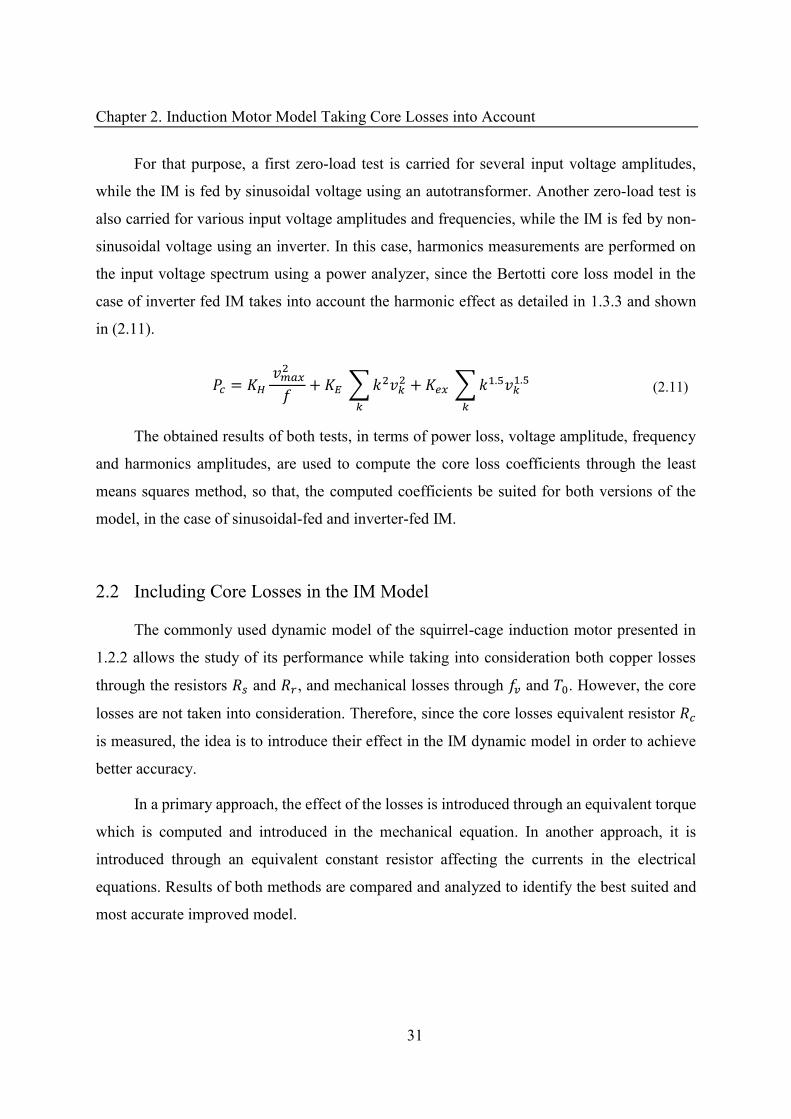
Chapter 2. Induction Motor Model Taking Core Losses into Account
31
For that purpose, a first zero-load test is carried for several input voltage amplitudes,
while the IM is fed by sinusoidal voltage using an autotransformer. Another zero-load test is
also carried for various input voltage amplitudes and frequencies, while the IM is fed by non-
sinusoidal voltage using an inverter. In this case, harmonics measurements are performed on
the input voltage spectrum using a power analyzer, since the Bertotti core loss model in the
case of inverter fed IM takes into account the harmonic effect as detailed in 1.3.3 and shown
in (2.11).
= � � + ∑ � � + � ∑ .5 �.5
� (2.11)
The obtained results of both tests, in terms of power loss, voltage amplitude, frequency
and harmonics amplitudes, are used to compute the core loss coefficients through the least
means squares method, so that, the computed coefficients be suited for both versions of the
model, in the case of sinusoidal-fed and inverter-fed IM.
2.2 Including Core Losses in the IM Model
The commonly used dynamic model of the squirrel-cage induction motor presented in
1.2.2 allows the study of its performance while taking into consideration both copper losses
through the resistors and , and mechanical losses through � and . However, the core
losses are not taken into consideration. Therefore, since the core losses equivalent resistor
is measured, the idea is to introduce their effect in the IM dynamic model in order to achieve
better accuracy.
In a primary approach, the effect of the losses is introduced through an equivalent torque
which is computed and introduced in the mechanical equation. In another approach, it is
introduced through an equivalent constant resistor affecting the currents in the electrical
equations. Results of both methods are compared and analyzed to identify the best suited and
most accurate improved model.
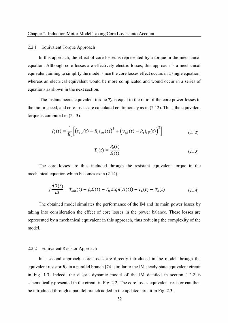
Chapter 2. Induction Motor Model Taking Core Losses into Account
32
2.2.1 Equivalent Torque Approach
In this approach, the effect of core losses is represented by a torque in the mechanical
equation. Although core losses are effectively electric losses, this approach is a mechanical
equivalent aiming to simplify the model since the core losses effect occurs in a single equation,
whereas an electrical equivalent would be more complicated and would occur in a series of
equations as shown in the next section.
The instantaneous equivalent torque is equal to the ratio of the core power losses to
the motor speed, and core losses are calculated continuously as in (2.12). Thus, the equivalent
torque is computed in (2.13).
= [( − ) + − ] (2.12)
= � (2.13)
The core losses are thus included through the resistant equivalent torque in the
mechanical equation which becomes as in (2.14). � = − �� − � − − (2.14)
The obtained model simulates the performance of the IM and its main power losses by
taking into consideration the effect of core losses in the power balance. These losses are
represented by a mechanical equivalent in this approach, thus reducing the complexity of the
model.
2.2.2 Equivalent Resistor Approach
In a second approach, core losses are directly introduced in the model through the
equivalent resistor in a parallel branch [74] similar to the IM steady-state equivalent circuit
in Fig. 1.3. Indeed, the classic dynamic model of the IM detailed in section 1.2.2 is
schematically presented in the circuit in Fig. 2.2. The core losses equivalent resistor can then
be introduced through a parallel branch added in the updated circuit in Fig. 2.3.
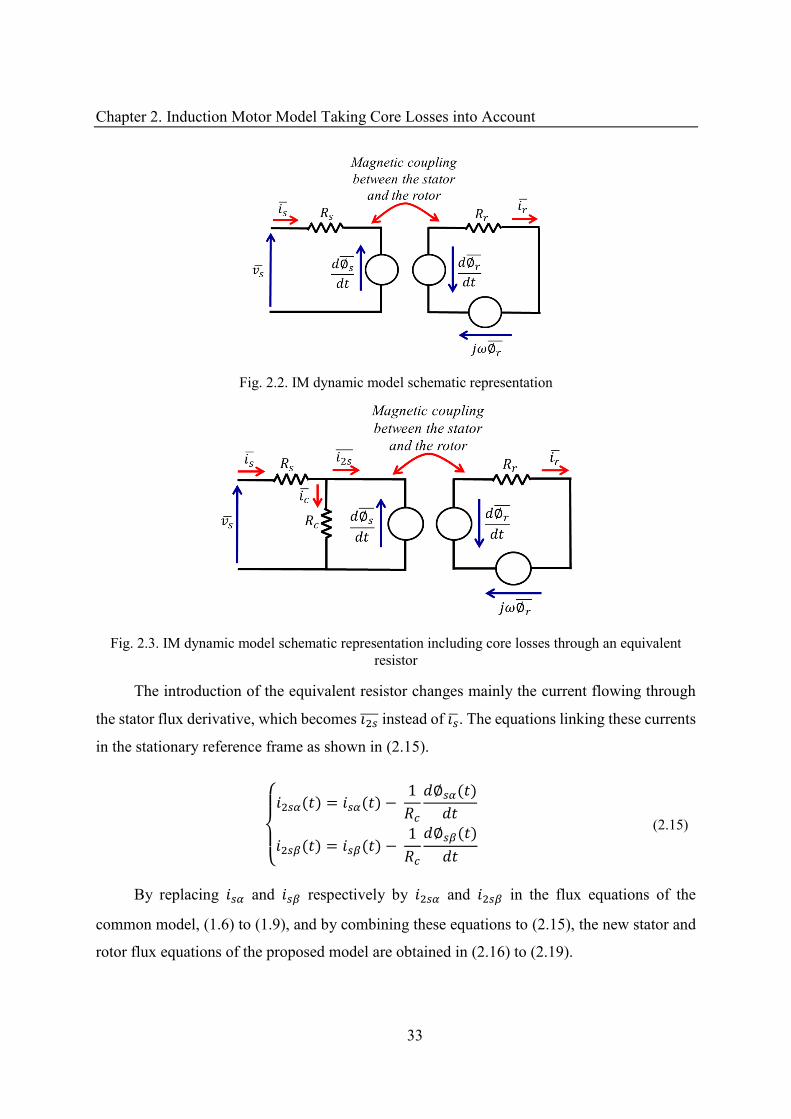
Chapter 2. Induction Motor Model Taking Core Losses into Account
33
Fig. 2.2. IM dynamic model schematic representation
Fig. 2.3. IM dynamic model schematic representation including core losses through an equivalent resistor
The introduction of the equivalent resistor changes mainly the current flowing through
the stator flux derivative, which becomes � instead of � . The equations linking these currents
in the stationary reference frame as shown in (2.15).
{ = − ∅
= − ∅ (2.15)
By replacing and respectively by and in the flux equations of the
common model, (1.6) to (1.9), and by combining these equations to (2.15), the new stator and
rotor flux equations of the proposed model are obtained in (2.16) to (2.19).
Chapter 2. Induction Motor Model Taking Core Losses into Account
34
∅ = − ∅ + (2.16)
∅ = − ∅ + (2.17)
∅ = + − ∅ (2.18)
∅ = + − ∅ (2.19)
The electrical and mechanical equations in the commonly used IM dynamic model, (1.2)
to (1.5), are not modified because the added branch does not affect the voltage, and the current
through the stator resistance is unchanged.
This model simulates the performance of the motor by taking into consideration the main
losses, in the power balance through the introduction of an electrical equivalent. It complicates
the model by introducing flux derivatives in the electrical flux equations.
2.2.3 Summary and Analysis
The introduction of the effect of core losses in the dynamic model of the IM has been
proposed through two approaches based on the equivalent resistor which is measured
through tests on the motor, thus, introducing the effect of these losses in the power balance.
Indeed, in the first method, the losses are represented mechanically by an equivalent torque
included in the mechanical equation, and in the other method the equivalent resistor is directly
used in the electrical equations of the model.
It is obvious that the representation of core losses through a resistor is closer to reality
than the use of the equivalent torque, because they exist in the motor as current losses in the
magnetic circuit of the stator and the rotor. This might cause differences in the simulation of
torque and speed, in the case of equivalent torque, because of the electrical loss introduced as
a disturbance in the mechanical equation. On the other hand, the equivalent resistor approach
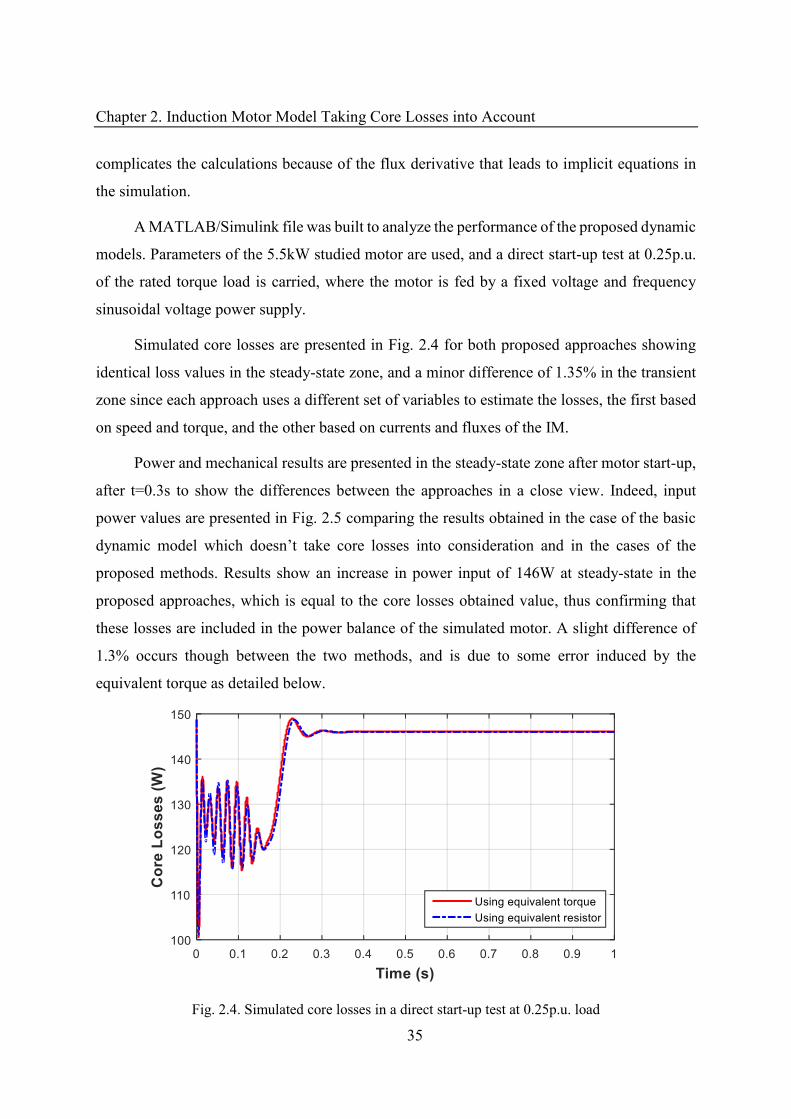
Chapter 2. Induction Motor Model Taking Core Losses into Account
35
complicates the calculations because of the flux derivative that leads to implicit equations in
the simulation.
A MATLAB/Simulink file was built to analyze the performance of the proposed dynamic
models. Parameters of the 5.5kW studied motor are used, and a direct start-up test at 0.25p.u.
of the rated torque load is carried, where the motor is fed by a fixed voltage and frequency
sinusoidal voltage power supply.
Simulated core losses are presented in Fig. 2.4 for both proposed approaches showing
identical loss values in the steady-state zone, and a minor difference of 1.35% in the transient
zone since each approach uses a different set of variables to estimate the losses, the first based
on speed and torque, and the other based on currents and fluxes of the IM.
Power and mechanical results are presented in the steady-state zone after motor start-up,
after t=0.3s to show the differences between the approaches in a close view. Indeed, input
power values are presented in Fig. 2.5 comparing the results obtained in the case of the basic
dynamic model which doesn’t take core losses into consideration and in the cases of the
proposed methods. Results show an increase in power input of 146W at steady-state in the
proposed approaches, which is equal to the core losses obtained value, thus confirming that
these losses are included in the power balance of the simulated motor. A slight difference of
1.3% occurs though between the two methods, and is due to some error induced by the
equivalent torque as detailed below.
Fig. 2.4. Simulated core losses in a direct start-up test at 0.25p.u. load
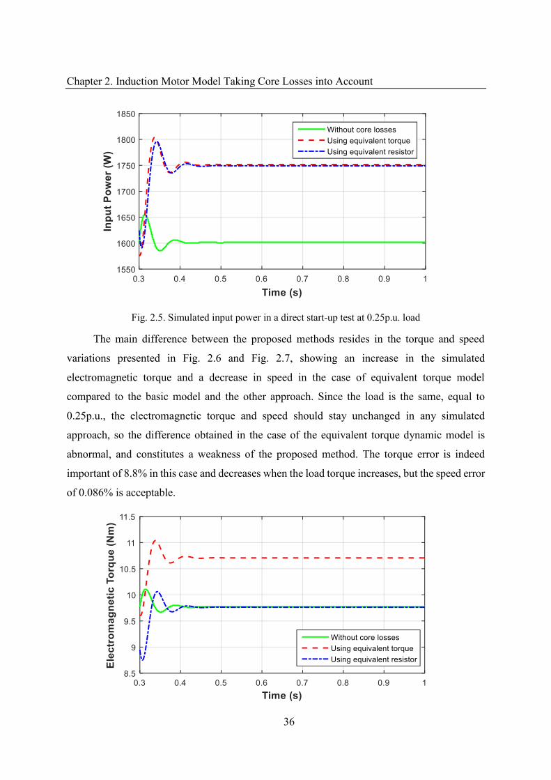
Chapter 2. Induction Motor Model Taking Core Losses into Account
36
Fig. 2.5. Simulated input power in a direct start-up test at 0.25p.u. load
The main difference between the proposed methods resides in the torque and speed
variations presented in Fig. 2.6 and Fig. 2.7, showing an increase in the simulated
electromagnetic torque and a decrease in speed in the case of equivalent torque model
compared to the basic model and the other approach. Since the load is the same, equal to
0.25p.u., the electromagnetic torque and speed should stay unchanged in any simulated
approach, so the difference obtained in the case of the equivalent torque dynamic model is
abnormal, and constitutes a weakness of the proposed method. The torque error is indeed
important of 8.8% in this case and decreases when the load torque increases, but the speed error
of 0.086% is acceptable.
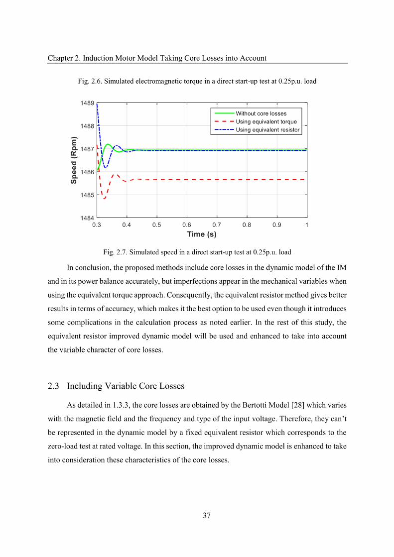
Chapter 2. Induction Motor Model Taking Core Losses into Account
37
Fig. 2.6. Simulated electromagnetic torque in a direct start-up test at 0.25p.u. load
Fig. 2.7. Simulated speed in a direct start-up test at 0.25p.u. load
In conclusion, the proposed methods include core losses in the dynamic model of the IM
and in its power balance accurately, but imperfections appear in the mechanical variables when
using the equivalent torque approach. Consequently, the equivalent resistor method gives better
results in terms of accuracy, which makes it the best option to be used even though it introduces
some complications in the calculation process as noted earlier. In the rest of this study, the
equivalent resistor improved dynamic model will be used and enhanced to take into account
the variable character of core losses.
2.3 Including Variable Core Losses
As detailed in 1.3.3, the core losses are obtained by the Bertotti Model [28] which varies
with the magnetic field and the frequency and type of the input voltage. Therefore, they can’t
be represented in the dynamic model by a fixed equivalent resistor which corresponds to the
zero-load test at rated voltage. In this section, the improved dynamic model is enhanced to take
into consideration these characteristics of the core losses.
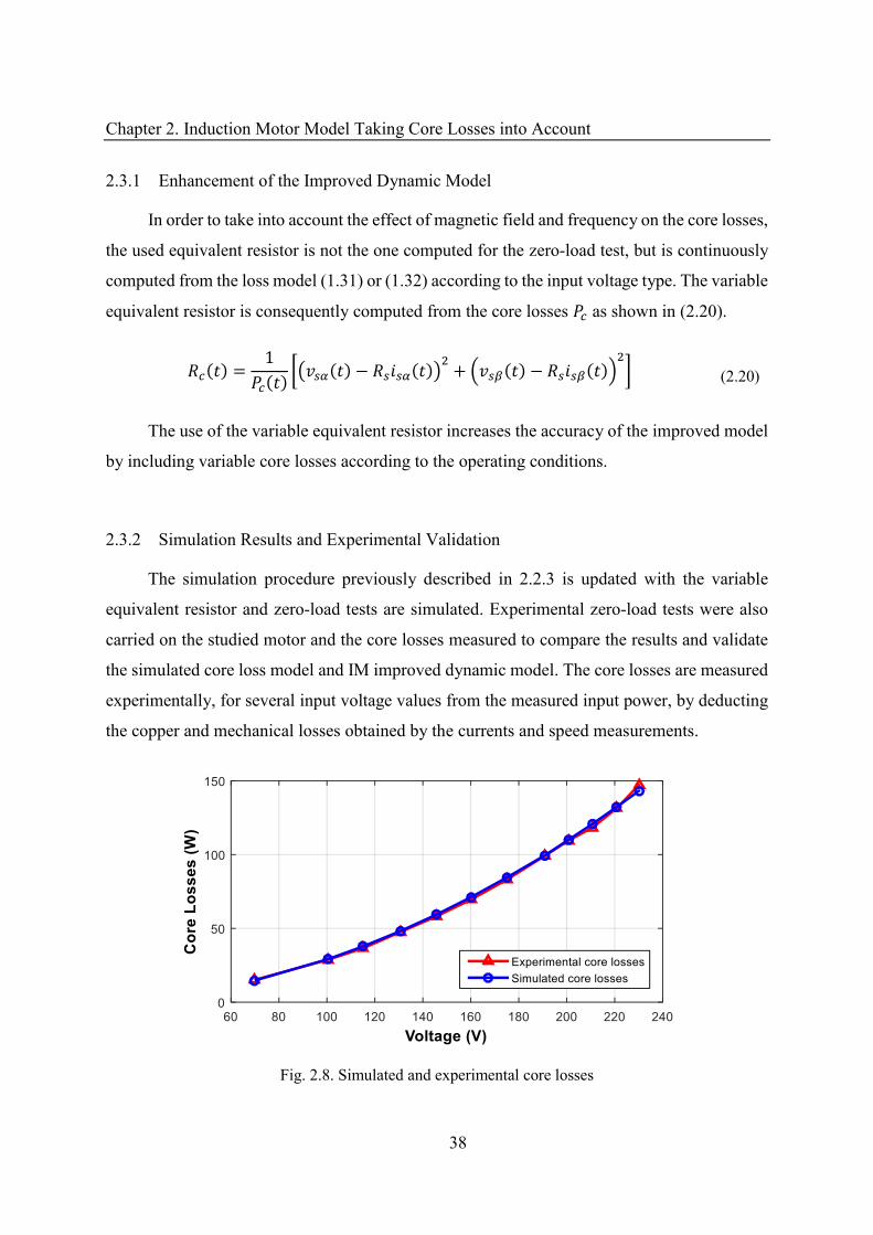
Chapter 2. Induction Motor Model Taking Core Losses into Account
38
2.3.1 Enhancement of the Improved Dynamic Model
In order to take into account the effect of magnetic field and frequency on the core losses,
the used equivalent resistor is not the one computed for the zero-load test, but is continuously
computed from the loss model (1.31) or (1.32) according to the input voltage type. The variable
equivalent resistor is consequently computed from the core losses as shown in (2.20).
= [( − ) + − ] (2.20)
The use of the variable equivalent resistor increases the accuracy of the improved model
by including variable core losses according to the operating conditions.
2.3.2 Simulation Results and Experimental Validation
The simulation procedure previously described in 2.2.3 is updated with the variable
equivalent resistor and zero-load tests are simulated. Experimental zero-load tests were also
carried on the studied motor and the core losses measured to compare the results and validate
the simulated core loss model and IM improved dynamic model. The core losses are measured
experimentally, for several input voltage values from the measured input power, by deducting
the copper and mechanical losses obtained by the currents and speed measurements.
Fig. 2.8. Simulated and experimental core losses
Chapter 2. Induction Motor Model Taking Core Losses into Account
39
The simulation and experimental results are shown in Fig. 2.8, they validate the proposed
dynamic model including variable core losses since the differences are minor and acceptable
with an average error of 1.84% between both curves.
Conclusion
The introduction of core losses in the dynamic model of the squirrel-cage induction motor
can be accomplished by two approaches, one of which is by creating a core loss equivalent
torque affecting the mechanical equation, and the other by using the core loss equivalent
resistor affecting the electrical equations. The second approach is proven to give more accurate
results compared to the first one which affects the simulated mechanical variables, thus the
equivalent resistor technique will be used in the rest of this study. This method is also enhanced
using a variable core loss equivalent resistor, which takes into consideration the effect of
magnetic field and frequency on the core losses, to increase the model accuracy.
The established model allows an accurate simulation of the induction motor, and can be
used for performance prediction of specific operating conditions. In the next chapter, the
improved model is used to compute the best efficiency points of the IM to be applied in a
further study to the control systems in order to increase energy efficiency.
Chapter 3 Best Efficiency Point Tracking
Table of Contents
Introduction ................................................................................................................ 41
3.1 Efficiency Computation ................................................................................. 41
3.1.1 Improved Dynamic Model in Complex Form ............................................ 41
3.1.2 Efficiency Equations ................................................................................... 43
3.2 Efficiency Mapping ........................................................................................ 45
3.2.1 Energy Efficiency Curves ........................................................................... 45
3.2.2 Energy Efficiency Plans ............................................................................. 48
3.3 Efficiency Optimization Approach ................................................................ 50
3.3.1 Optimal Flux ............................................................................................... 50
3.3.2 Load Torque Observer ................................................................................ 53
Conclusion .................................................................................................................. 55
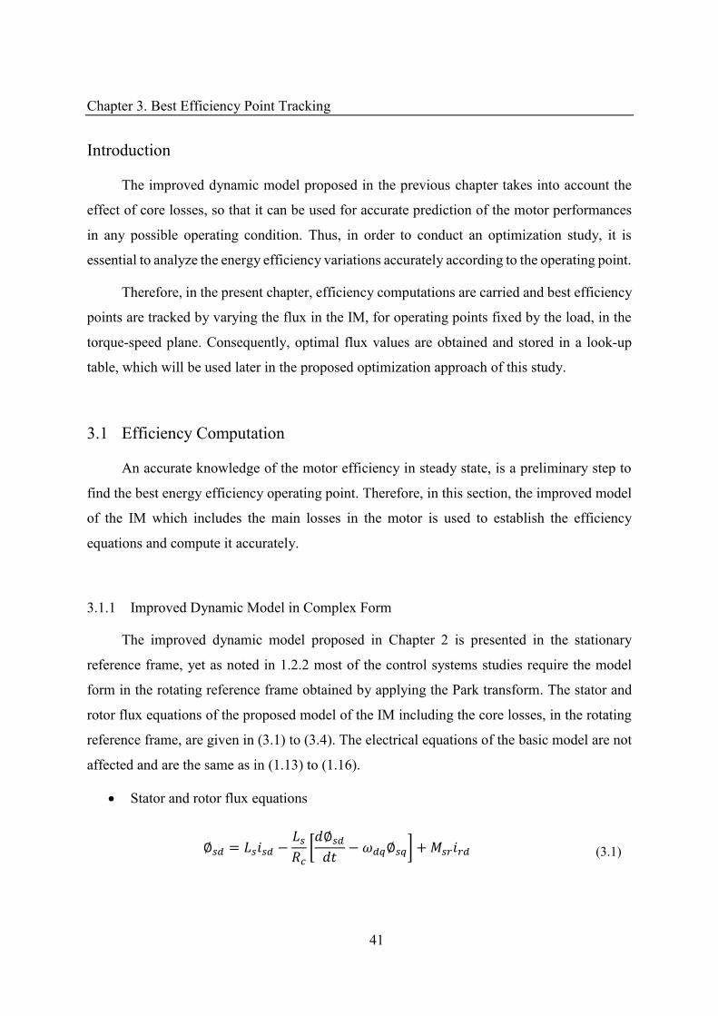
Chapter 3. Best Efficiency Point Tracking
41
Introduction
The improved dynamic model proposed in the previous chapter takes into account the
effect of core losses, so that it can be used for accurate prediction of the motor performances
in any possible operating condition. Thus, in order to conduct an optimization study, it is
essential to analyze the energy efficiency variations accurately according to the operating point.
Therefore, in the present chapter, efficiency computations are carried and best efficiency
points are tracked by varying the flux in the IM, for operating points fixed by the load, in the
torque-speed plane. Consequently, optimal flux values are obtained and stored in a look-up
table, which will be used later in the proposed optimization approach of this study.
3.1 Efficiency Computation
An accurate knowledge of the motor efficiency in steady state, is a preliminary step to
find the best energy efficiency operating point. Therefore, in this section, the improved model
of the IM which includes the main losses in the motor is used to establish the efficiency
equations and compute it accurately.
3.1.1 Improved Dynamic Model in Complex Form
The improved dynamic model proposed in Chapter 2 is presented in the stationary
reference frame, yet as noted in 1.2.2 most of the control systems studies require the model
form in the rotating reference frame obtained by applying the Park transform. The stator and
rotor flux equations of the proposed model of the IM including the core losses, in the rotating
reference frame, are given in (3.1) to (3.4). The electrical equations of the basic model are not
affected and are the same as in (1.13) to (1.16).
• Stator and rotor flux equations
∅ = − [ ∅ − � ∅ ] + (3.1)
Chapter 3. Best Efficiency Point Tracking
42
∅ = − [ ∅ + � ∅ ] + (3.2)
∅ = + − [ ∅ − � ∅ ] (3.3)
∅ = + − [ ∅ + � ∅ ] (3.4)
� represents the angular speed of the − rotating frame. The study is carried at
steady state rotating sinusoidal operating mode, where the angular frequency of the reference
frame � is equal to the stator angular frequency � , and thus, the equation (3.5) between the
stator and rotor angular frequency � is verified. � = � − � (3.5)
In order to compute the energy efficiency, the input power and electromagnetic torque
are calculated. Hence, the dynamic model is written in complex form by combining each − couple of equations into one complex phasor as shown in (3.6) to (3.9), using the relation = + defining the space vector for each variable .
• The stator electrical equation
= � + � ∅ (3.6)
• The rotor electrical equation
= � + � ∅ (3.7)
• The stator flux equation
∅ = � − � ∅ + � (3.8)
Chapter 3. Best Efficiency Point Tracking
43
• The rotor flux equation
∅ = � + � − � ∅ (3.9)
This model is used in the following section to compute energy efficiency as a function
of the stator or the rotor flux.
3.1.2 Efficiency Equations
The energy efficiency is the ratio of the output power to the input power � , which is
computed through (3.10) where is the electromagnetic torque.
� = .Ω −� (3.10)
Knowing that the Concordia transform, which preserves power values, is used in this
study to obtain the model in the stationary reference frame, the input power [16] is computed
in (3.11) and the electromagnetic torque in (3.12), where ∗ is the conjugate of the space
phasor.
� = . � ∗ (3.11) = . . � . � ∗ (3.12)
The mechanical losses are computed according to equation (1.25), and the calculation of
the input power and electromagnetic torque are conducted using the stator voltage and currents space
phasors from the improved dynamic model of the IM in complex form. These calculations can
be done to represent the efficiency as a function of the stator flux or as a function of the rotor
flux, a choice to be made depending on the application or the control structure.
In a first approach, calculations are done according to the stator flux. Equations (3.13)
and (3.14) relating the stator and rotor currents to the stator flux are therefore established, and
the efficiency variation can be identified according to the stator flux.
Chapter 3. Best Efficiency Point Tracking
44
� = − � � �
+ � + � + � � ∅ (3.13)
� = − � �+ � ∅ − �+ � � (3.14)
In the other approach, the stator and rotor currents are written as functions of the rotor
flux as in (3.15) to (3.17), so that the efficiency variations can be assessed according to the
rotor flux.
� = − � ∅ (3.15)
� = ( + � ) ∅ + � ∅ (3.16)
∅ = ( + � � ) ∅ (3.17)
In both approaches, the flux and stator angular frequency are provided by the user or
control system, according to the operating conditions required, whereas the torque is fixed by
the load. Therefore, the angular frequency � is obtained by resolving the motor torque
equation (3.18) at steady state, when the electromagnetic torque equals the sum of the load
demand and the mechanical losses. = �� + + (3.18)
Once the rotor angular frequency computed, as well as the input power (3.10) and
electromagnetic torque (3.11), the motor energy efficiency is calculated (3.12).
Chapter 3. Best Efficiency Point Tracking
45
3.2 Efficiency Mapping
The energy efficiency model obtained depends on the operating conditions and the
required load. Hence, it is possible to predict the best efficiency point by computing the
efficiency values at all possible operating points.
A simulation file is established to perform the necessary calculations for a wide range of
operating points of the studied IE2 5.5kW IM presented in 2.1, in a way to track the best
efficiency point. According to the model presented in 3.1, the variables affecting the energy
efficiency are the flux, the load torque and the speed of the motor. Consequently, efficiency
numbers are computed for several values of flux, load and speed to map the efficiency
variations and track the optimal operating point.
3.2.1 Energy Efficiency Curves
In a first approach, efficiency variations are evaluated for variable stator flux and fixed
load torques and speeds. For this purpose, the improved model detailed in 3.1 in steady-state
is used to calculate the currents by scanning the possible flux values, for given speed and torque
values, then the efficiency is computed. Results are shown in the graphs in Fig. 3.1 to Fig. 3.4
for different torques in per unit of the rated torque, and different speeds in per unit of the base
speed. The curves show that the optimal operating point at maximum efficiency is not always
obtained at rated flux. Indeed, for load torque values less than 0.6p.u. as shown in Fig. 3.1 to
Fig. 3.3 at base speed, the optimal stator flux values can reach 0.4p.u. flux, and 0.2p.u. in the
case of zero-load test. On the other hand, in the case of load torques greater than 0.6p.u., the
rated flux corresponds to the optimal operating point as shown in Fig. 3.4.
These optimal points are affected by the rotating speed as it appears in the graphs, as for
instance at 0.2p.u. speed, the optimal point corresponds to the rated flux for loads above 0.3p.u.
torque.
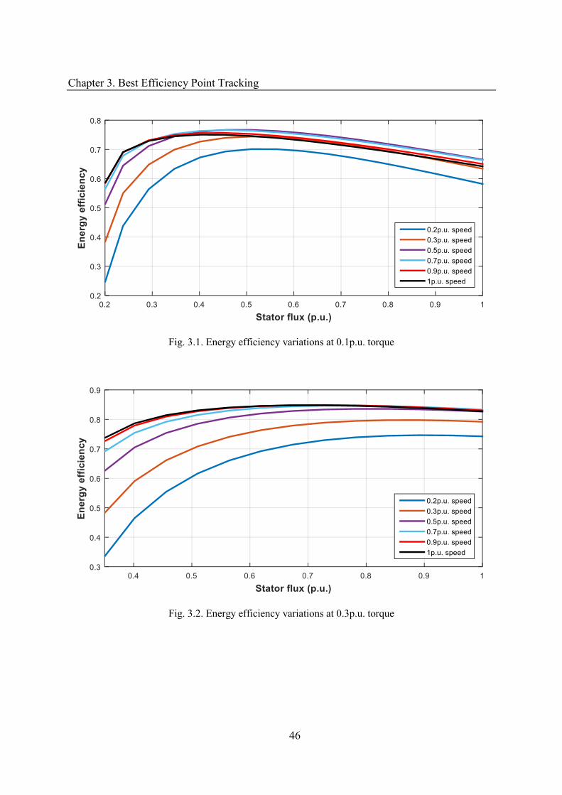
Chapter 3. Best Efficiency Point Tracking
46
Fig. 3.1. Energy efficiency variations at 0.1p.u. torque
Fig. 3.2. Energy efficiency variations at 0.3p.u. torque
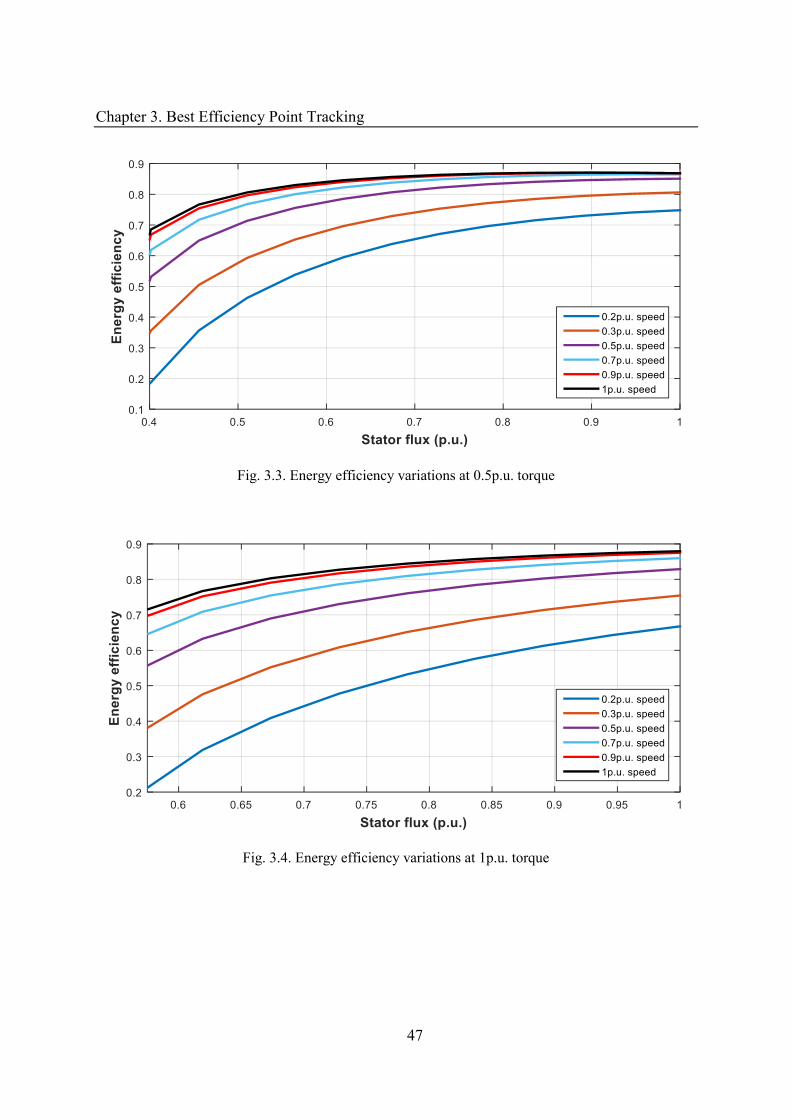
Chapter 3. Best Efficiency Point Tracking
47
Fig. 3.3. Energy efficiency variations at 0.5p.u. torque
Fig. 3.4. Energy efficiency variations at 1p.u. torque
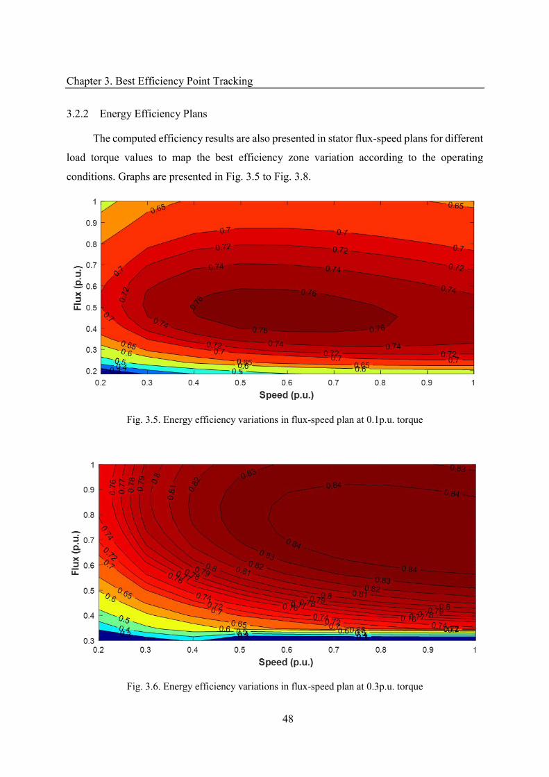
Chapter 3. Best Efficiency Point Tracking
48
3.2.2 Energy Efficiency Plans
The computed efficiency results are also presented in stator flux-speed plans for different
load torque values to map the best efficiency zone variation according to the operating
conditions. Graphs are presented in Fig. 3.5 to Fig. 3.8.
Fig. 3.5. Energy efficiency variations in flux-speed plan at 0.1p.u. torque
Fig. 3.6. Energy efficiency variations in flux-speed plan at 0.3p.u. torque
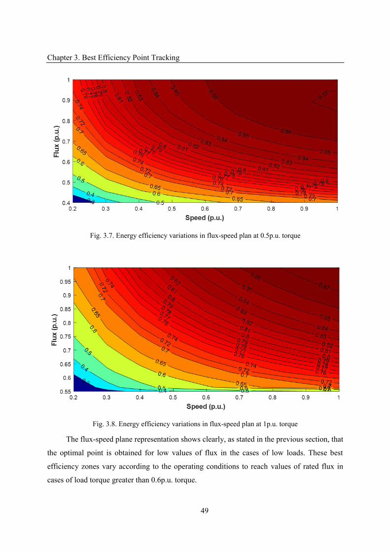
Chapter 3. Best Efficiency Point Tracking
49
Fig. 3.7. Energy efficiency variations in flux-speed plan at 0.5p.u. torque
Fig. 3.8. Energy efficiency variations in flux-speed plan at 1p.u. torque
The flux-speed plane representation shows clearly, as stated in the previous section, that
the optimal point is obtained for low values of flux in the cases of low loads. These best
efficiency zones vary according to the operating conditions to reach values of rated flux in
cases of load torque greater than 0.6p.u. torque.
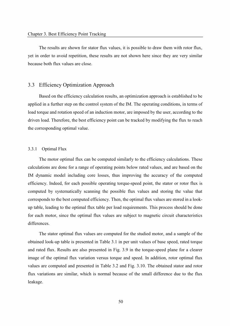
Chapter 3. Best Efficiency Point Tracking
50
The results are shown for stator flux values, it is possible to draw them with rotor flux,
yet in order to avoid repetition, these results are not shown here since they are very similar
because both flux values are close.
3.3 Efficiency Optimization Approach
Based on the efficiency calculation results, an optimization approach is established to be
applied in a further step on the control system of the IM. The operating conditions, in terms of
load torque and rotation speed of an induction motor, are imposed by the user, according to the
driven load. Therefore, the best efficiency point can be tracked by modifying the flux to reach
the corresponding optimal value.
3.3.1 Optimal Flux
The motor optimal flux can be computed similarly to the efficiency calculations. These
calculations are done for a range of operating points below rated values, and are based on the
IM dynamic model including core losses, thus improving the accuracy of the computed
efficiency. Indeed, for each possible operating torque-speed point, the stator or rotor flux is
computed by systematically scanning the possible flux values and storing the value that
corresponds to the best computed efficiency. Then, the optimal flux values are stored in a look-
up table, leading to the optimal flux table per load requirements. This process should be done
for each motor, since the optimal flux values are subject to magnetic circuit characteristics
differences.
The stator optimal flux values are computed for the studied motor, and a sample of the
obtained look-up table is presented in Table 3.1 in per unit values of base speed, rated torque
and rated flux. Results are also presented in Fig. 3.9 in the torque-speed plane for a clearer
image of the optimal flux variation versus torque and speed. In addition, rotor optimal flux
values are computed and presented in Table 3.2 and Fig. 3.10. The obtained stator and rotor
flux variations are similar, which is normal because of the small difference due to the flux
leakage.
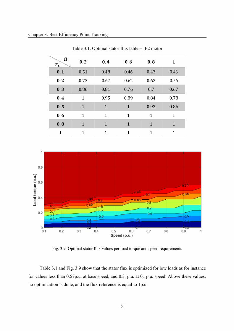
Chapter 3. Best Efficiency Point Tracking
51
Table 3.1. Optimal stator flux table – IE2 motor � �� . . . . . . . .46 . .43 . . .67 .62 . .56 . . . . . . . . . . . . . . . .
Fig. 3.9. Optimal stator flux values per load torque and speed requirements
Table 3.1 and Fig. 3.9 show that the stator flux is optimized for low loads as for instance
for values less than 0.57p.u. at base speed, and 0.31p.u. at 0.1p.u. speed. Above these values,
no optimization is done, and the flux reference is equal to 1p.u.
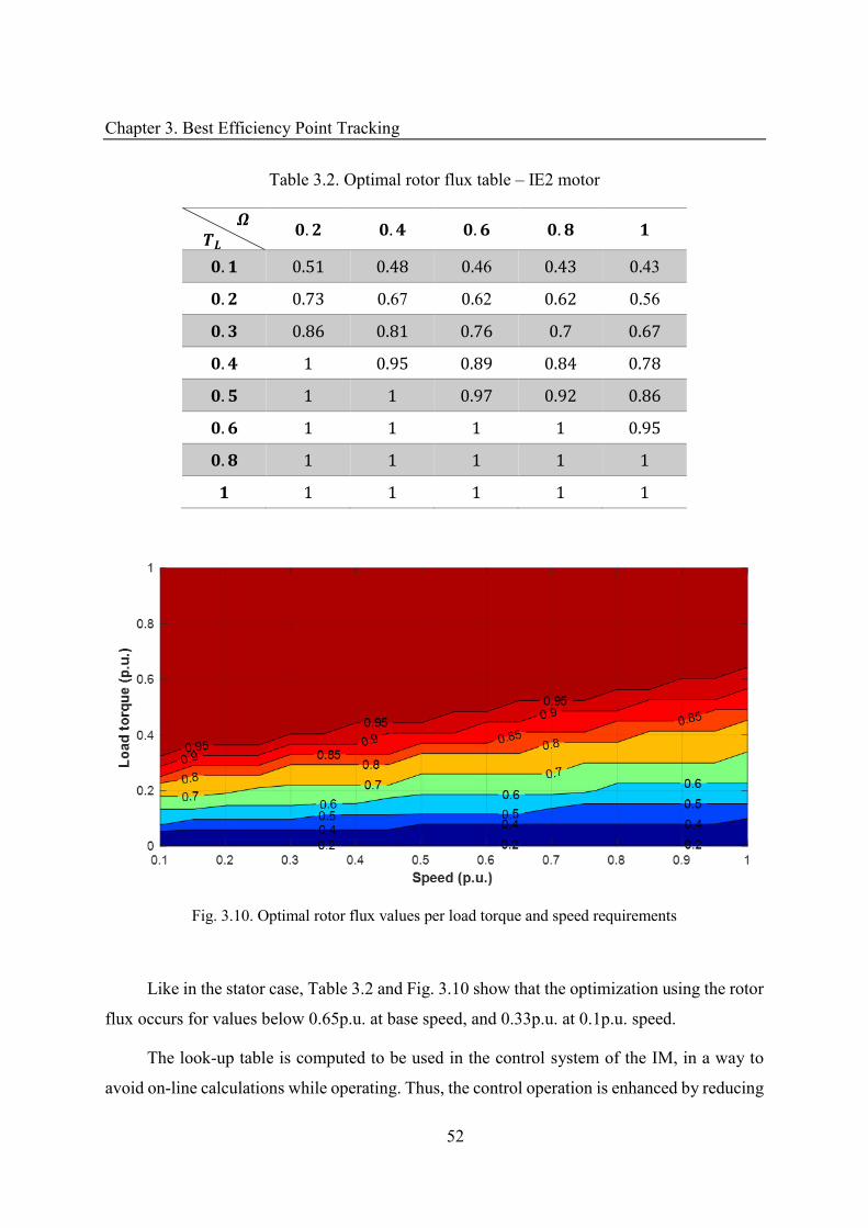
Chapter 3. Best Efficiency Point Tracking
52
Table 3.2. Optimal rotor flux table – IE2 motor � �� . . . . . . . .46 . .43 . . .67 .62 . .56 . . . . . . . . . . . . . . . . . .
Fig. 3.10. Optimal rotor flux values per load torque and speed requirements
Like in the stator case, Table 3.2 and Fig. 3.10 show that the optimization using the rotor
flux occurs for values below 0.65p.u. at base speed, and 0.33p.u. at 0.1p.u. speed.
The look-up table is computed to be used in the control system of the IM, in a way to
avoid on-line calculations while operating. Thus, the control operation is enhanced by reducing
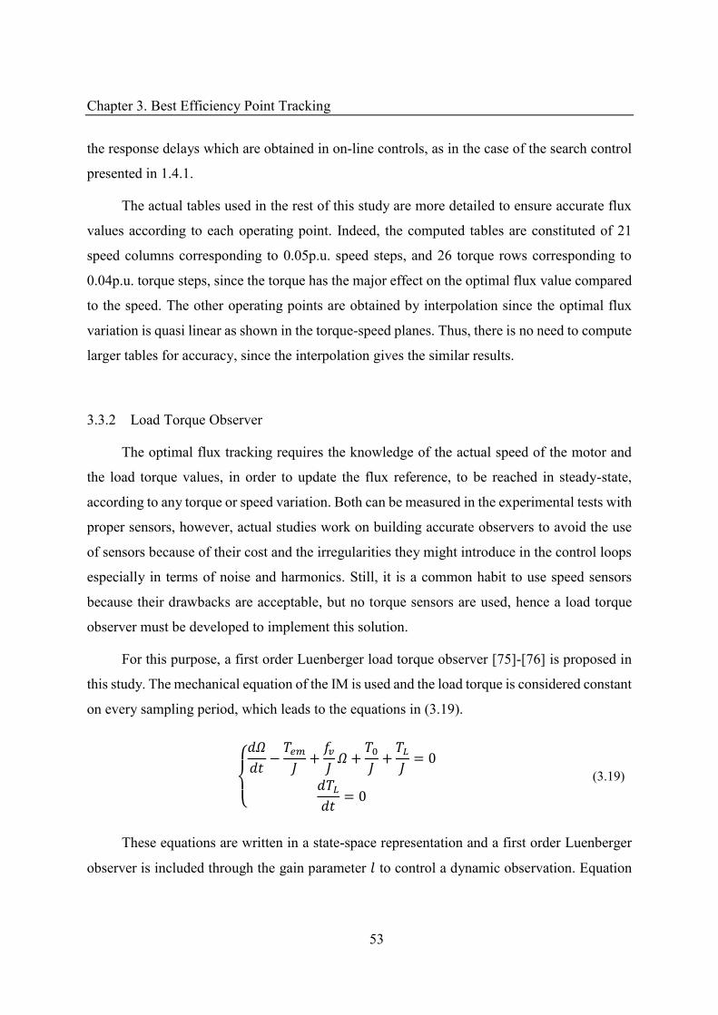
Chapter 3. Best Efficiency Point Tracking
53
the response delays which are obtained in on-line controls, as in the case of the search control
presented in 1.4.1.
The actual tables used in the rest of this study are more detailed to ensure accurate flux
values according to each operating point. Indeed, the computed tables are constituted of 21
speed columns corresponding to 0.05p.u. speed steps, and 26 torque rows corresponding to
0.04p.u. torque steps, since the torque has the major effect on the optimal flux value compared
to the speed. The other operating points are obtained by interpolation since the optimal flux
variation is quasi linear as shown in the torque-speed planes. Thus, there is no need to compute
larger tables for accuracy, since the interpolation gives the similar results.
3.3.2 Load Torque Observer
The optimal flux tracking requires the knowledge of the actual speed of the motor and
the load torque values, in order to update the flux reference, to be reached in steady-state,
according to any torque or speed variation. Both can be measured in the experimental tests with
proper sensors, however, actual studies work on building accurate observers to avoid the use
of sensors because of their cost and the irregularities they might introduce in the control loops
especially in terms of noise and harmonics. Still, it is a common habit to use speed sensors
because their drawbacks are acceptable, but no torque sensors are used, hence a load torque
observer must be developed to implement this solution.
For this purpose, a first order Luenberger load torque observer [75]-[76] is proposed in
this study. The mechanical equation of the IM is used and the load torque is considered constant
on every sampling period, which leads to the equations in (3.19).
{ � − + � � + + == (3.19)
These equations are written in a state-space representation and a first order Luenberger
observer is included through the gain parameter to control a dynamic observation. Equation
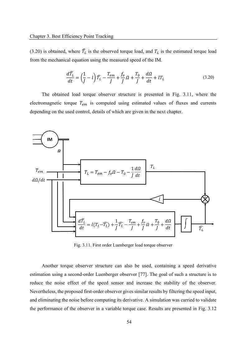
Chapter 3. Best Efficiency Point Tracking
54
(3.20) is obtained, where is the observed torque load, and is the estimated torque load
from the mechanical equation using the measured speed of the IM. = ( − ) − + � � + + � + (3.20)
The obtained load torque observer structure is presented in Fig. 3.11, where the
electromagnetic torque is computed using estimated values of fluxes and currents
depending on the used control, details of which are given in the next chapter.
Fig. 3.11. First order Luenberger load torque observer
Another torque observer structure can also be used, containing a speed derivative
estimation using a second-order Luenberger observer [77]. The goal of such a structure is to
reduce the noise effect of the speed sensor and increase the stability of the observer.
Nevertheless, the proposed first-order observer gives similar results by filtering the speed input,
and eliminating the noise before computing its derivative. A simulation was carried to validate
the performance of the observer in a variable torque case. Results are presented in Fig. 3.12
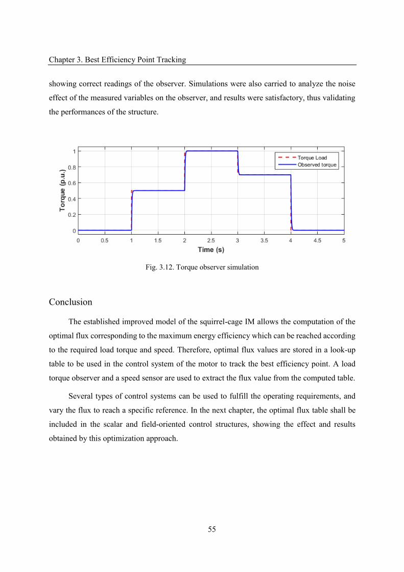
Chapter 3. Best Efficiency Point Tracking
55
showing correct readings of the observer. Simulations were also carried to analyze the noise
effect of the measured variables on the observer, and results were satisfactory, thus validating
the performances of the structure.
Fig. 3.12. Torque observer simulation
Conclusion
The established improved model of the squirrel-cage IM allows the computation of the
optimal flux corresponding to the maximum energy efficiency which can be reached according
to the required load torque and speed. Therefore, optimal flux values are stored in a look-up
table to be used in the control system of the motor to track the best efficiency point. A load
torque observer and a speed sensor are used to extract the flux value from the computed table.
Several types of control systems can be used to fulfill the operating requirements, and
vary the flux to reach a specific reference. In the next chapter, the optimal flux table shall be
included in the scalar and field-oriented control structures, showing the effect and results
obtained by this optimization approach.

Chapter 4 Control Systems Optimization
Table of Contents
Introduction ................................................................................................................ 57
4.1 Scalar Control Optimization........................................................................... 57
4.1.1 Classic Scalar Control Structure ................................................................. 57
4.1.2 Optimized Scalar Control ........................................................................... 59
4.1.3 Simulation and analysis .............................................................................. 61
4.2 Optimized Field-oriented Control .................................................................. 67
4.2.1 Classic field-oriented Control Structure ..................................................... 67
4.2.2 Optimized field-oriented Control ............................................................... 73
4.2.3 Simulation and analysis .............................................................................. 73
Conclusion .................................................................................................................. 78
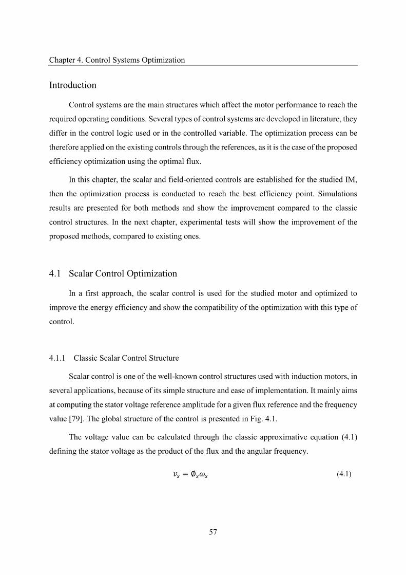
Chapter 4. Control Systems Optimization
57
Introduction
Control systems are the main structures which affect the motor performance to reach the
required operating conditions. Several types of control systems are developed in literature, they
differ in the control logic used or in the controlled variable. The optimization process can be
therefore applied on the existing controls through the references, as it is the case of the proposed
efficiency optimization using the optimal flux.
In this chapter, the scalar and field-oriented controls are established for the studied IM,
then the optimization process is conducted to reach the best efficiency point. Simulations
results are presented for both methods and show the improvement compared to the classic
control structures. In the next chapter, experimental tests will show the improvement of the
proposed methods, compared to existing ones.
4.1 Scalar Control Optimization
In a first approach, the scalar control is used for the studied motor and optimized to
improve the energy efficiency and show the compatibility of the optimization with this type of
control.
4.1.1 Classic Scalar Control Structure
Scalar control is one of the well-known control structures used with induction motors, in
several applications, because of its simple structure and ease of implementation. It mainly aims
at computing the stator voltage reference amplitude for a given flux reference and the frequency
value [79]. The global structure of the control is presented in Fig. 4.1.
The voltage value can be calculated through the classic approximative equation (4.1)
defining the stator voltage as the product of the flux and the angular frequency. = ∅ � (4.1)
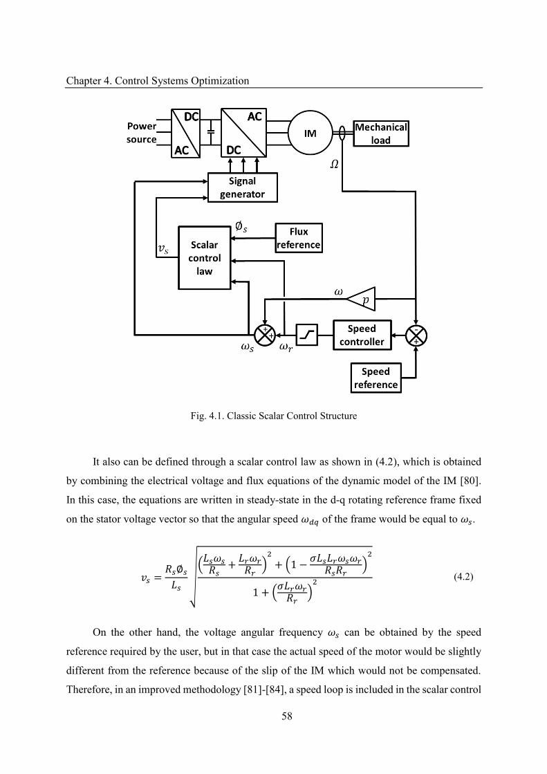
Chapter 4. Control Systems Optimization
58
Fig. 4.1. Classic Scalar Control Structure
It also can be defined through a scalar control law as shown in (4.2), which is obtained
by combining the electrical voltage and flux equations of the dynamic model of the IM [80].
In this case, the equations are written in steady-state in the d-q rotating reference frame fixed
on the stator voltage vector so that the angular speed � of the frame would be equal to � .
= ∅ √ � + � + − � � �+ � � (4.2)
On the other hand, the voltage angular frequency � can be obtained by the speed
reference required by the user, but in that case the actual speed of the motor would be slightly
different from the reference because of the slip of the IM which would not be compensated.
Therefore, in an improved methodology [81]-[84], a speed loop is included in the scalar control
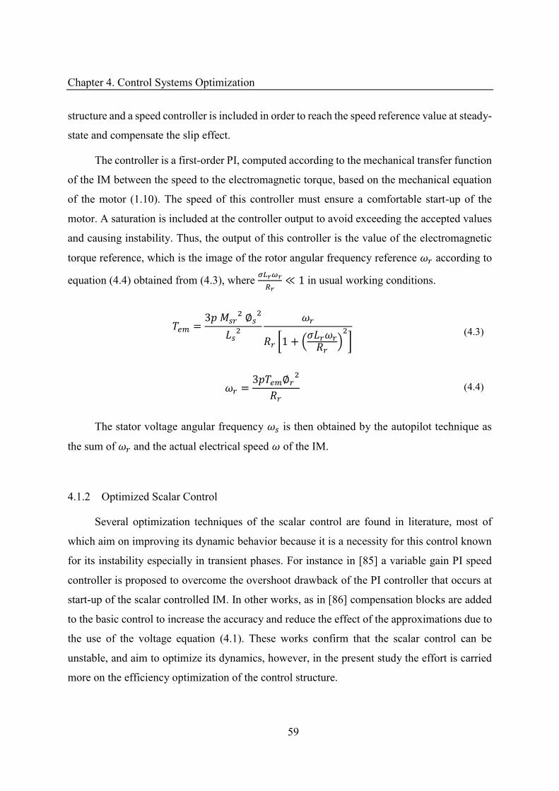
Chapter 4. Control Systems Optimization
59
structure and a speed controller is included in order to reach the speed reference value at steady-
state and compensate the slip effect.
The controller is a first-order PI, computed according to the mechanical transfer function
of the IM between the speed to the electromagnetic torque, based on the mechanical equation
of the motor (1.10). The speed of this controller must ensure a comfortable start-up of the
motor. A saturation is included at the controller output to avoid exceeding the accepted values
and causing instability. Thus, the output of this controller is the value of the electromagnetic
torque reference, which is the image of the rotor angular frequency reference � according to
equation (4.4) obtained from (4.3), where � �� ≪ in usual working conditions.
= ∅ �[ + � � ] (4.3)
� = ∅ (4.4)
The stator voltage angular frequency � is then obtained by the autopilot technique as
the sum of � and the actual electrical speed � of the IM.
4.1.2 Optimized Scalar Control
Several optimization techniques of the scalar control are found in literature, most of
which aim on improving its dynamic behavior because it is a necessity for this control known
for its instability especially in transient phases. For instance in [85] a variable gain PI speed
controller is proposed to overcome the overshoot drawback of the PI controller that occurs at
start-up of the scalar controlled IM. In other works, as in [86] compensation blocks are added
to the basic control to increase the accuracy and reduce the effect of the approximations due to
the use of the voltage equation (4.1). These works confirm that the scalar control can be
unstable, and aim to optimize its dynamics, however, in the present study the effort is carried
more on the efficiency optimization of the control structure.
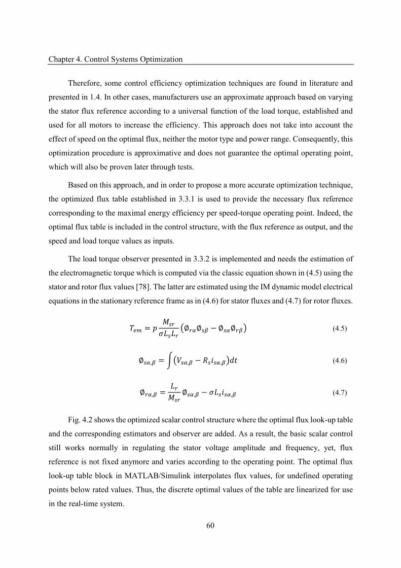
Chapter 4. Control Systems Optimization
60
Therefore, some control efficiency optimization techniques are found in literature and
presented in 1.4. In other cases, manufacturers use an approximate approach based on varying
the stator flux reference according to a universal function of the load torque, established and
used for all motors to increase the efficiency. This approach does not take into account the
effect of speed on the optimal flux, neither the motor type and power range. Consequently, this
optimization procedure is approximative and does not guarantee the optimal operating point,
which will also be proven later through tests.
Based on this approach, and in order to propose a more accurate optimization technique,
the optimized flux table established in 3.3.1 is used to provide the necessary flux reference
corresponding to the maximal energy efficiency per speed-torque operating point. Indeed, the
optimal flux table is included in the control structure, with the flux reference as output, and the
speed and load torque values as inputs.
The load torque observer presented in 3.3.2 is implemented and needs the estimation of
the electromagnetic torque which is computed via the classic equation shown in (4.5) using the
stator and rotor flux values [78]. The latter are estimated using the IM dynamic model electrical
equations in the stationary reference frame as in (4.6) for stator fluxes and (4.7) for rotor fluxes.
= � (∅ ∅ − ∅ ∅ ) (4.5)
∅ , = ∫( , − , ) (4.6)
∅ , = ∅ , − � , (4.7)
Fig. 4.2 shows the optimized scalar control structure where the optimal flux look-up table
and the corresponding estimators and observer are added. As a result, the basic scalar control
still works normally in regulating the stator voltage amplitude and frequency, yet, flux
reference is not fixed anymore and varies according to the operating point. The optimal flux
look-up table block in MATLAB/Simulink interpolates flux values, for undefined operating
points below rated values. Thus, the discrete optimal values of the table are linearized for use
in the real-time system.
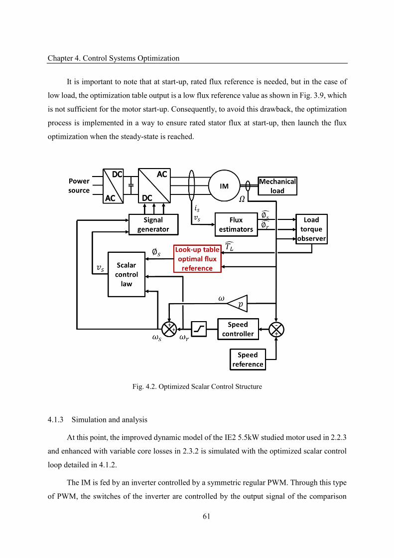
Chapter 4. Control Systems Optimization
61
It is important to note that at start-up, rated flux reference is needed, but in the case of
low load, the optimization table output is a low flux reference value as shown in Fig. 3.9, which
is not sufficient for the motor start-up. Consequently, to avoid this drawback, the optimization
process is implemented in a way to ensure rated stator flux at start-up, then launch the flux
optimization when the steady-state is reached.
Fig. 4.2. Optimized Scalar Control Structure
4.1.3 Simulation and analysis
At this point, the improved dynamic model of the IE2 5.5kW studied motor used in 2.2.3
and enhanced with variable core losses in 2.3.2 is simulated with the optimized scalar control
loop detailed in 4.1.2.
The IM is fed by an inverter controlled by a symmetric regular PWM. Through this type
of PWM, the switches of the inverter are controlled by the output signal of the comparison
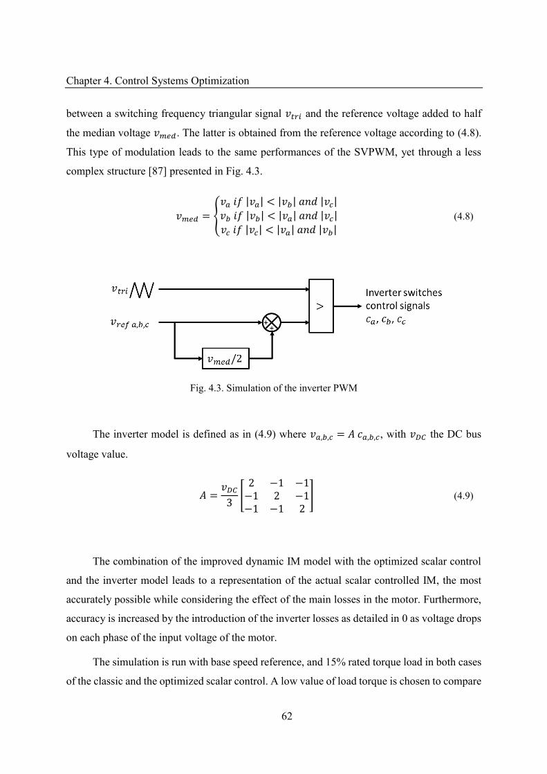
Chapter 4. Control Systems Optimization
62
between a switching frequency triangular signal � and the reference voltage added to half
the median voltage . The latter is obtained from the reference voltage according to (4.8).
This type of modulation leads to the same performances of the SVPWM, yet through a less
complex structure [87] presented in Fig. 4.3.
= { | | < | | | | | | < | | | | | | < | | | | (4.8)
Fig. 4.3. Simulation of the inverter PWM
The inverter model is defined as in (4.9) where , , = , , , with the DC bus
voltage value.
= [ − −− −− − ] (4.9)
The combination of the improved dynamic IM model with the optimized scalar control
and the inverter model leads to a representation of the actual scalar controlled IM, the most
accurately possible while considering the effect of the main losses in the motor. Furthermore,
accuracy is increased by the introduction of the inverter losses as detailed in 0 as voltage drops
on each phase of the input voltage of the motor.
The simulation is run with base speed reference, and 15% rated torque load in both cases
of the classic and the optimized scalar control. A low value of load torque is chosen to compare
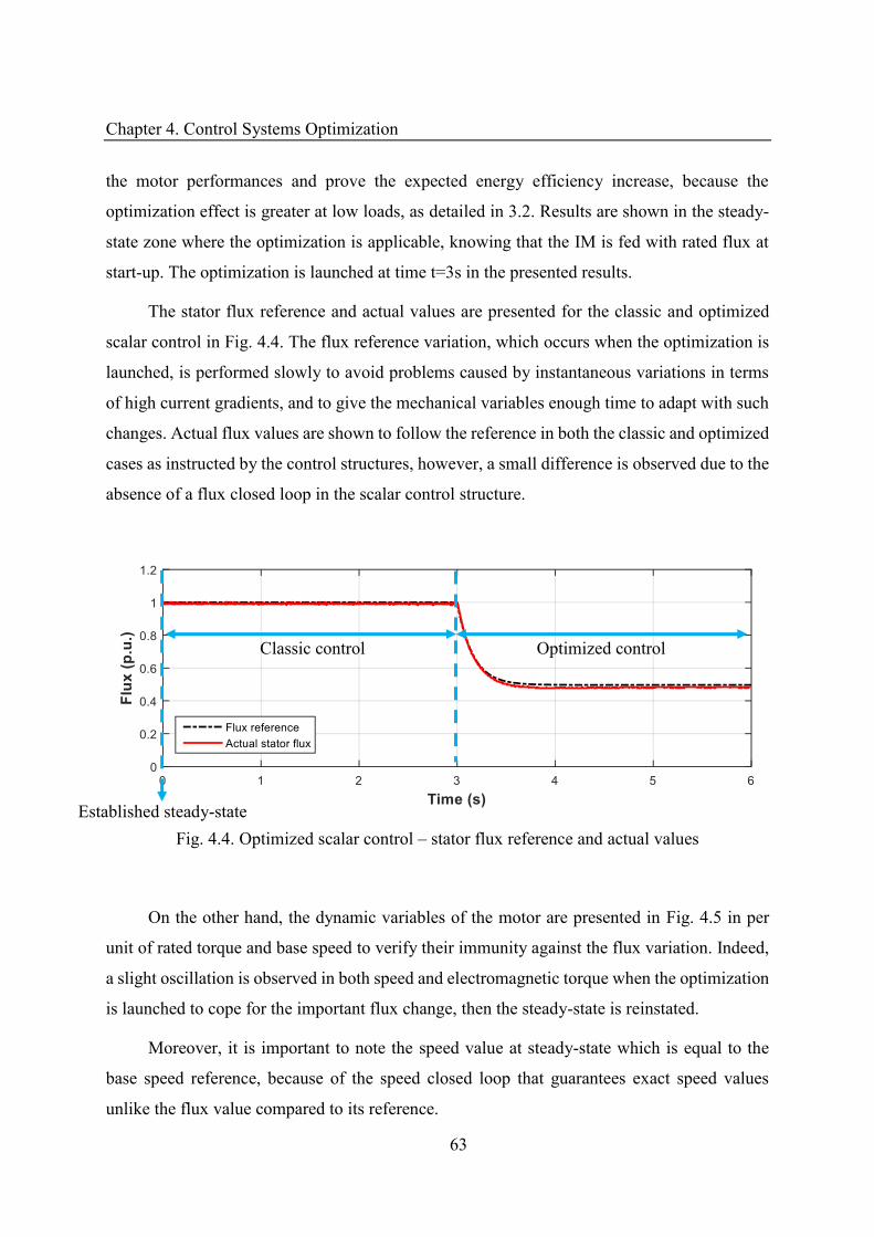
Chapter 4. Control Systems Optimization
63
the motor performances and prove the expected energy efficiency increase, because the
optimization effect is greater at low loads, as detailed in 3.2. Results are shown in the steady-
state zone where the optimization is applicable, knowing that the IM is fed with rated flux at
start-up. The optimization is launched at time t=3s in the presented results.
The stator flux reference and actual values are presented for the classic and optimized
scalar control in Fig. 4.4. The flux reference variation, which occurs when the optimization is
launched, is performed slowly to avoid problems caused by instantaneous variations in terms
of high current gradients, and to give the mechanical variables enough time to adapt with such
changes. Actual flux values are shown to follow the reference in both the classic and optimized
cases as instructed by the control structures, however, a small difference is observed due to the
absence of a flux closed loop in the scalar control structure.
Fig. 4.4. Optimized scalar control – stator flux reference and actual values
On the other hand, the dynamic variables of the motor are presented in Fig. 4.5 in per
unit of rated torque and base speed to verify their immunity against the flux variation. Indeed,
a slight oscillation is observed in both speed and electromagnetic torque when the optimization
is launched to cope for the important flux change, then the steady-state is reinstated.
Moreover, it is important to note the speed value at steady-state which is equal to the
base speed reference, because of the speed closed loop that guarantees exact speed values
unlike the flux value compared to its reference.
Classic control Optimized control
Established steady-state
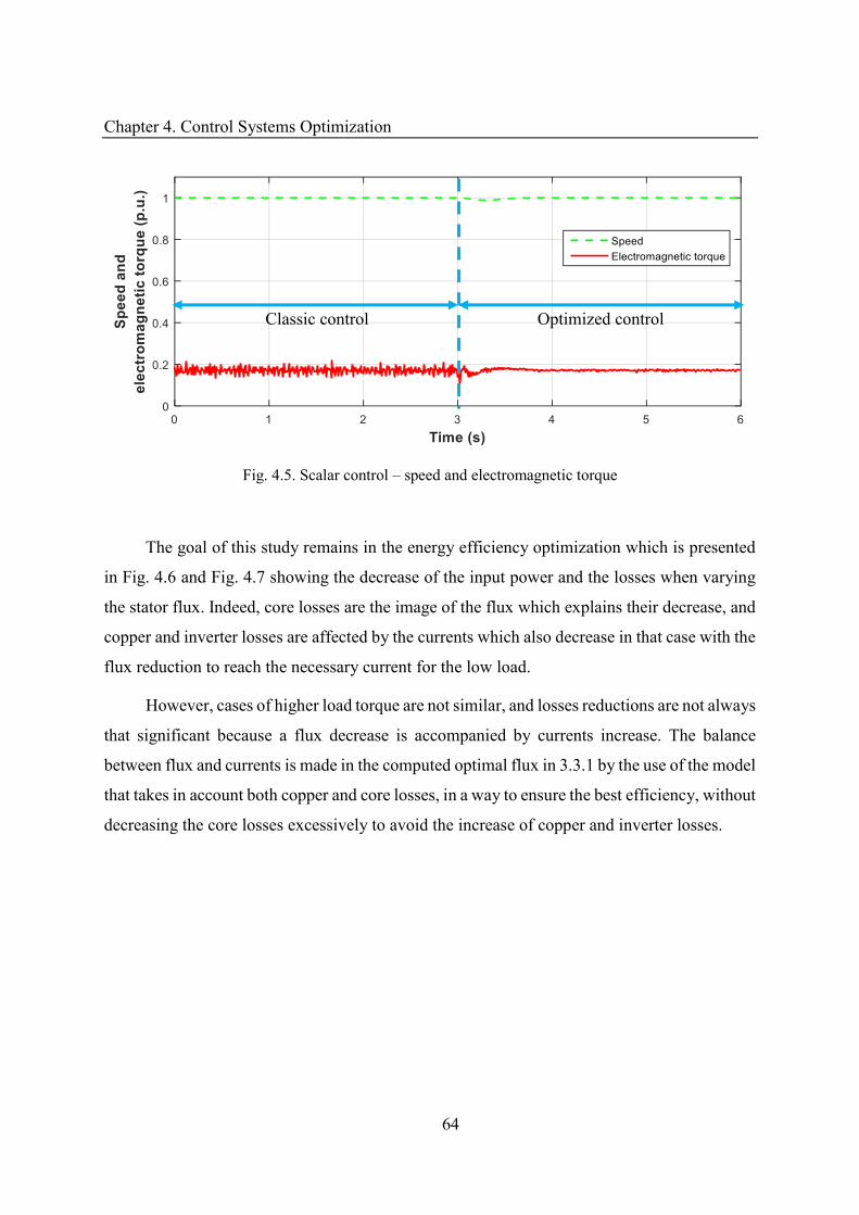
Chapter 4. Control Systems Optimization
64
Fig. 4.5. Scalar control – speed and electromagnetic torque
The goal of this study remains in the energy efficiency optimization which is presented
in Fig. 4.6 and Fig. 4.7 showing the decrease of the input power and the losses when varying
the stator flux. Indeed, core losses are the image of the flux which explains their decrease, and
copper and inverter losses are affected by the currents which also decrease in that case with the
flux reduction to reach the necessary current for the low load.
However, cases of higher load torque are not similar, and losses reductions are not always
that significant because a flux decrease is accompanied by currents increase. The balance
between flux and currents is made in the computed optimal flux in 3.3.1 by the use of the model
that takes in account both copper and core losses, in a way to ensure the best efficiency, without
decreasing the core losses excessively to avoid the increase of copper and inverter losses.
Classic control Optimized control
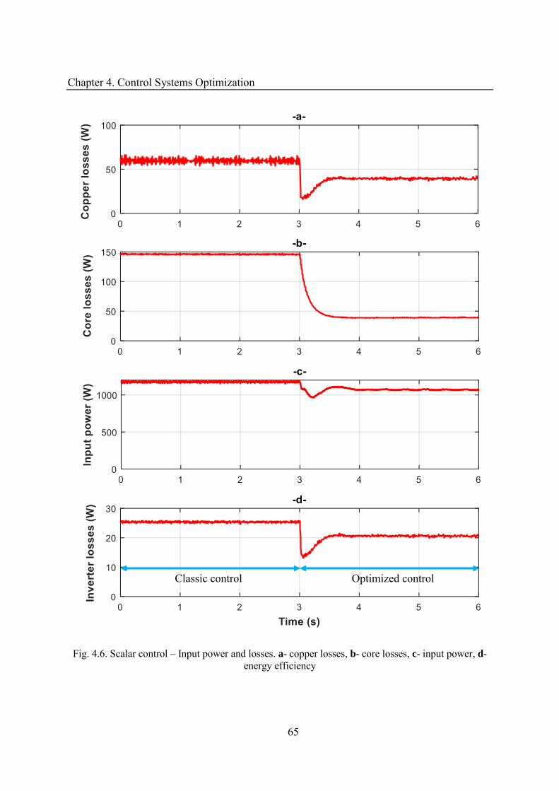
Chapter 4. Control Systems Optimization
65
Fig. 4.6. Scalar control – Input power and losses. a- copper losses, b- core losses, c- input power, d- energy efficiency
Classic control Optimized control
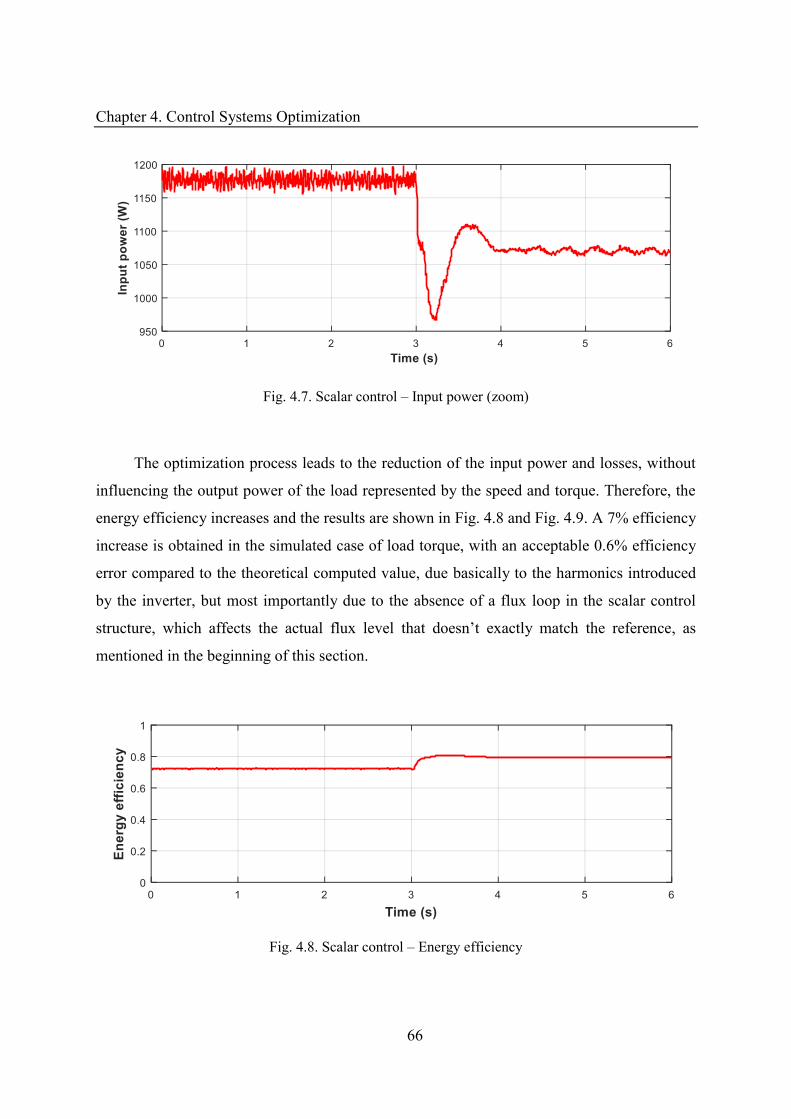
Chapter 4. Control Systems Optimization
66
Fig. 4.7. Scalar control – Input power (zoom)
The optimization process leads to the reduction of the input power and losses, without
influencing the output power of the load represented by the speed and torque. Therefore, the
energy efficiency increases and the results are shown in Fig. 4.8 and Fig. 4.9. A 7% efficiency
increase is obtained in the simulated case of load torque, with an acceptable 0.6% efficiency
error compared to the theoretical computed value, due basically to the harmonics introduced
by the inverter, but most importantly due to the absence of a flux loop in the scalar control
structure, which affects the actual flux level that doesn’t exactly match the reference, as
mentioned in the beginning of this section.
Fig. 4.8. Scalar control – Energy efficiency
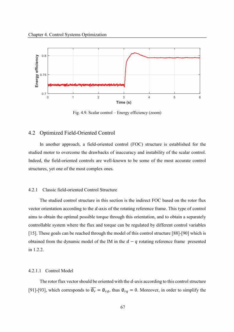
Chapter 4. Control Systems Optimization
67
Fig. 4.9. Scalar control – Energy efficiency (zoom)
4.2 Optimized Field-Oriented Control
In another approach, a field-oriented control (FOC) structure is established for the
studied motor to overcome the drawbacks of inaccuracy and instability of the scalar control.
Indeed, the field-oriented controls are well-known to be some of the most accurate control
structures, yet one of the most complex ones.
4.2.1 Classic field-oriented Control Structure
The studied control structure in this section is the indirect FOC based on the rotor flux
vector orientation according to the -axis of the rotating reference frame. This type of control
aims to obtain the optimal possible torque through this orientation, and to obtain a separately
controllable system where the flux and torque can be regulated by different control variables
[15]. These goals can be reached through the model of this control structure [88]-[90] which is
obtained from the dynamic model of the IM in the − rotating reference frame presented
in 1.2.2.
4.2.1.1 Control Model
The rotor flux vector should be oriented with the -axis according to this control structure
[91]-[93], which corresponds to ∅ = ∅ , thus ∅ = . Moreover, in order to simplify the
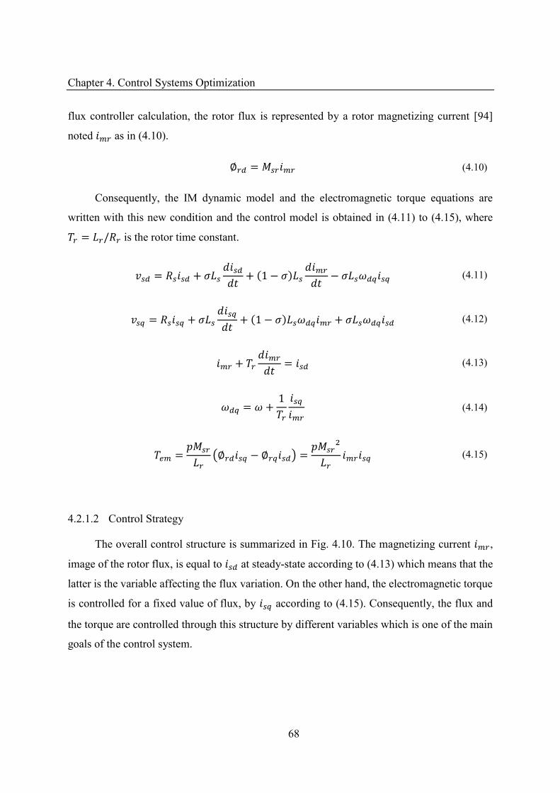
Chapter 4. Control Systems Optimization
68
flux controller calculation, the rotor flux is represented by a rotor magnetizing current [94]
noted as in (4.10). ∅ = (4.10)
Consequently, the IM dynamic model and the electromagnetic torque equations are
written with this new condition and the control model is obtained in (4.11) to (4.15), where = / is the rotor time constant.
= + � + − � − � � (4.11)
= + � + − � � + � � (4.12)
+ = (4.13)
� = � + (4.14)
= (∅ − ∅ ) = (4.15)
4.2.1.2 Control Strategy
The overall control structure is summarized in Fig. 4.10. The magnetizing current ,
image of the rotor flux, is equal to at steady-state according to (4.13) which means that the
latter is the variable affecting the flux variation. On the other hand, the electromagnetic torque
is controlled for a fixed value of flux, by according to (4.15). Consequently, the flux and
the torque are controlled through this structure by different variables which is one of the main
goals of the control system.
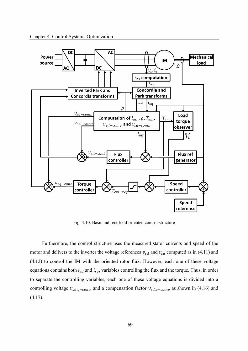
Chapter 4. Control Systems Optimization
69
Fig. 4.10. Basic indirect field-oriented control structure
Furthermore, the control structure uses the measured stator currents and speed of the
motor and delivers to the inverter the voltage references and computed as in (4.11) and
(4.12) to control the IM with the oriented rotor flux. However, each one of these voltage
equations contains both and , variables controlling the flux and the torque. Thus, in order
to separate the controlling variables, each one of these voltage equations is divided into a
controlling voltage , − , and a compensation factor , − as shown in (4.16) and
(4.17).
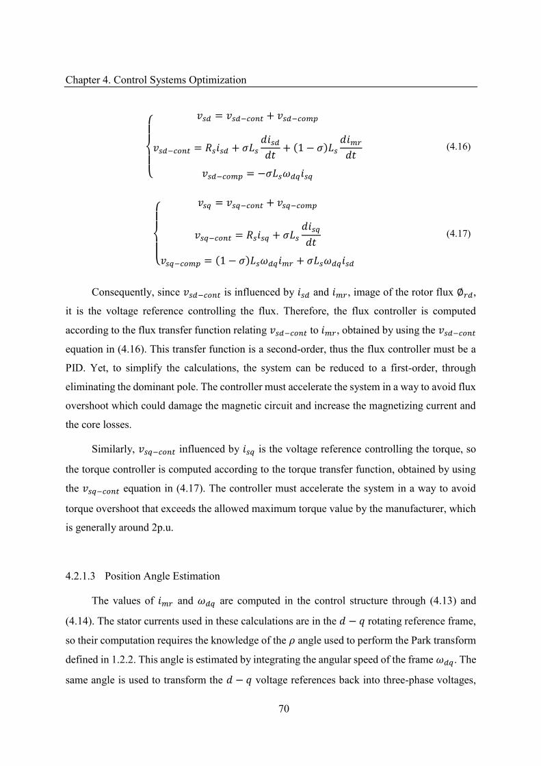
Chapter 4. Control Systems Optimization
70
{ = − + − − = + � + − � − = −� � (4.16)
{ = − + −
− = + � − = − � � + � � (4.17)
Consequently, since − is influenced by and , image of the rotor flux ∅ ,
it is the voltage reference controlling the flux. Therefore, the flux controller is computed
according to the flux transfer function relating − to , obtained by using the −
equation in (4.16). This transfer function is a second-order, thus the flux controller must be a
PID. Yet, to simplify the calculations, the system can be reduced to a first-order, through
eliminating the dominant pole. The controller must accelerate the system in a way to avoid flux
overshoot which could damage the magnetic circuit and increase the magnetizing current and
the core losses.
Similarly, − influenced by is the voltage reference controlling the torque, so
the torque controller is computed according to the torque transfer function, obtained by using
the − equation in (4.17). The controller must accelerate the system in a way to avoid
torque overshoot that exceeds the allowed maximum torque value by the manufacturer, which
is generally around 2p.u.
4.2.1.3 Position Angle Estimation
The values of and � are computed in the control structure through (4.13) and
(4.14). The stator currents used in these calculations are in the − rotating reference frame,
so their computation requires the knowledge of the � angle used to perform the Park transform
defined in 1.2.2. This angle is estimated by integrating the angular speed of the frame � . The
same angle is used to transform the − voltage references back into three-phase voltages,
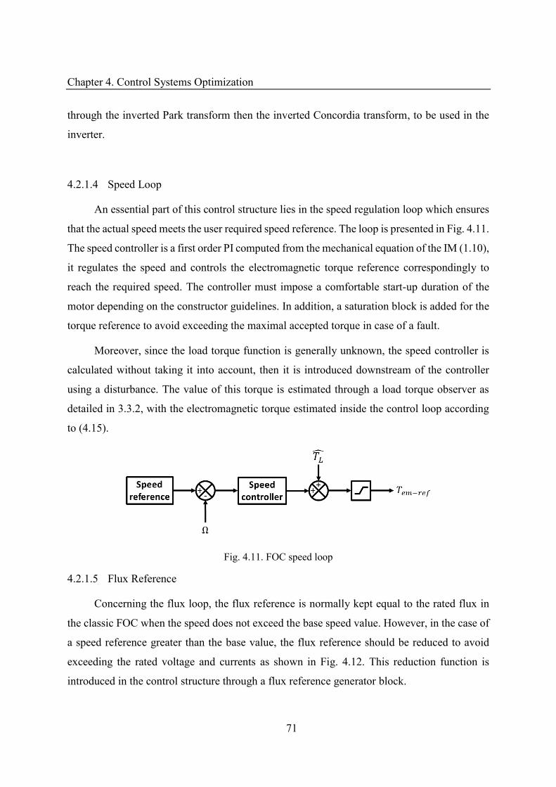
Chapter 4. Control Systems Optimization
71
through the inverted Park transform then the inverted Concordia transform, to be used in the
inverter.
4.2.1.4 Speed Loop
An essential part of this control structure lies in the speed regulation loop which ensures
that the actual speed meets the user required speed reference. The loop is presented in Fig. 4.11.
The speed controller is a first order PI computed from the mechanical equation of the IM (1.10),
it regulates the speed and controls the electromagnetic torque reference correspondingly to
reach the required speed. The controller must impose a comfortable start-up duration of the
motor depending on the constructor guidelines. In addition, a saturation block is added for the
torque reference to avoid exceeding the maximal accepted torque in case of a fault.
Moreover, since the load torque function is generally unknown, the speed controller is
calculated without taking it into account, then it is introduced downstream of the controller
using a disturbance. The value of this torque is estimated through a load torque observer as
detailed in 3.3.2, with the electromagnetic torque estimated inside the control loop according
to (4.15).
Fig. 4.11. FOC speed loop
4.2.1.5 Flux Reference
Concerning the flux loop, the flux reference is normally kept equal to the rated flux in
the classic FOC when the speed does not exceed the base speed value. However, in the case of
a speed reference greater than the base value, the flux reference should be reduced to avoid
exceeding the rated voltage and currents as shown in Fig. 4.12. This reduction function is
introduced in the control structure through a flux reference generator block.
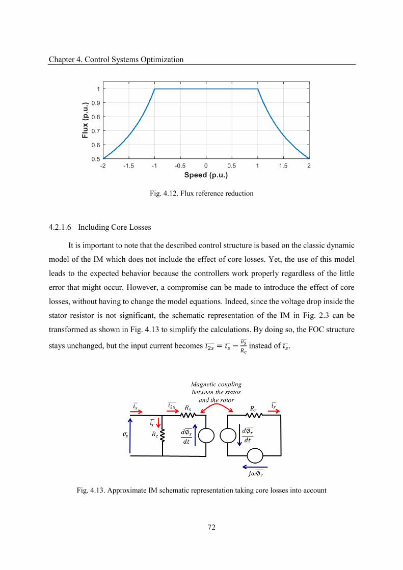
Chapter 4. Control Systems Optimization
72
Fig. 4.12. Flux reference reduction
4.2.1.6 Including Core Losses
It is important to note that the described control structure is based on the classic dynamic
model of the IM which does not include the effect of core losses. Yet, the use of this model
leads to the expected behavior because the controllers work properly regardless of the little
error that might occur. However, a compromise can be made to introduce the effect of core
losses, without having to change the model equations. Indeed, since the voltage drop inside the
stator resistor is not significant, the schematic representation of the IM in Fig. 2.3 can be
transformed as shown in Fig. 4.13 to simplify the calculations. By doing so, the FOC structure
stays unchanged, but the input current becomes � = � − ��� instead of � .
Fig. 4.13. Approximate IM schematic representation taking core losses into account
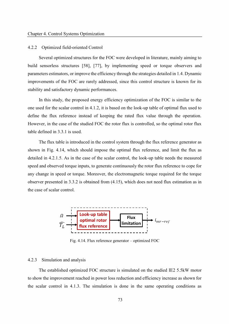
Chapter 4. Control Systems Optimization
73
4.2.2 Optimized field-oriented Control
Several optimized structures for the FOC were developed in literature, mainly aiming to
build sensorless structures [58], [77], by implementing speed or torque observers and
parameters estimators, or improve the efficiency through the strategies detailed in 1.4. Dynamic
improvements of the FOC are rarely addressed, since this control structure is known for its
stability and satisfactory dynamic performances.
In this study, the proposed energy efficiency optimization of the FOC is similar to the
one used for the scalar control in 4.1.2, it is based on the look-up table of optimal flux used to
define the flux reference instead of keeping the rated flux value through the operation.
However, in the case of the studied FOC the rotor flux is controlled, so the optimal rotor flux
table defined in 3.3.1 is used.
The flux table is introduced in the control system through the flux reference generator as
shown in Fig. 4.14, which should impose the optimal flux reference, and limit the flux as
detailed in 4.2.1.5. As in the case of the scalar control, the look-up table needs the measured
speed and observed torque inputs, to generate continuously the rotor flux reference to cope for
any change in speed or torque. Moreover, the electromagnetic torque required for the torque
observer presented in 3.3.2 is obtained from (4.15), which does not need flux estimation as in
the case of scalar control.
Fig. 4.14. Flux reference generator – optimized FOC
4.2.3 Simulation and analysis
The established optimized FOC structure is simulated on the studied IE2 5.5kW motor
to show the improvement reached in power loss reduction and efficiency increase as shown for
the scalar control in 4.1.3. The simulation is done in the same operating conditions as
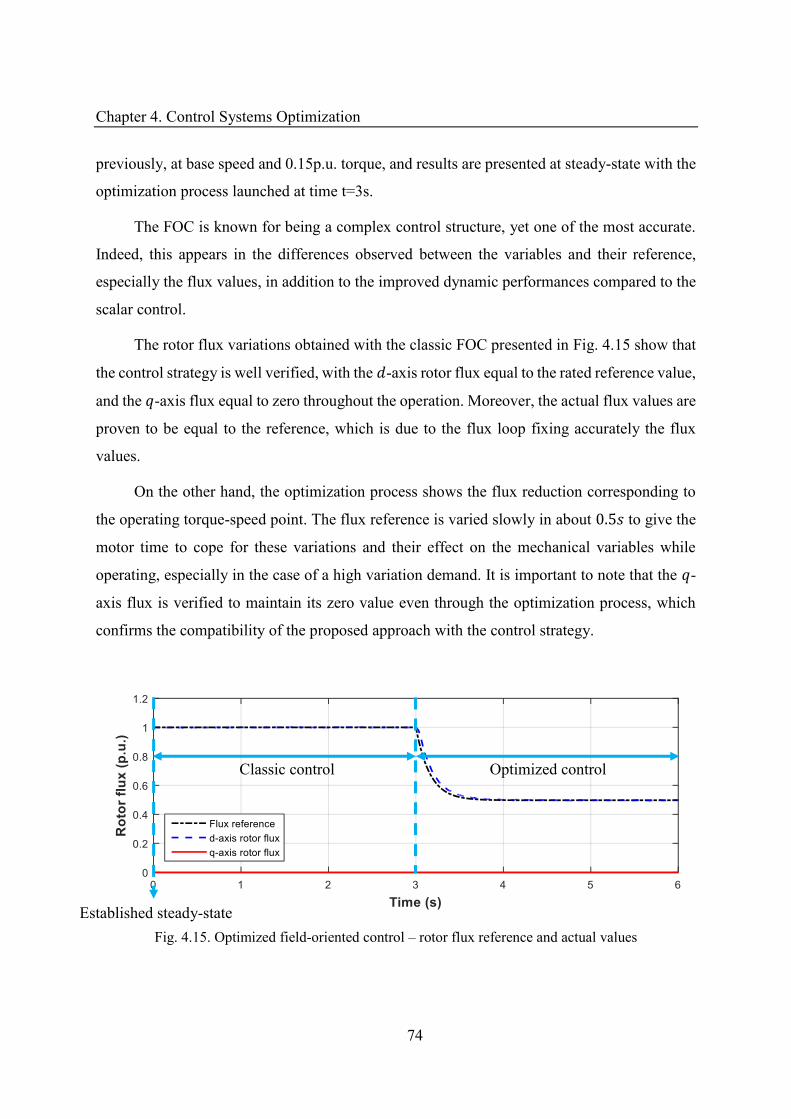
Chapter 4. Control Systems Optimization
74
previously, at base speed and 0.15p.u. torque, and results are presented at steady-state with the
optimization process launched at time t=3s.
The FOC is known for being a complex control structure, yet one of the most accurate.
Indeed, this appears in the differences observed between the variables and their reference,
especially the flux values, in addition to the improved dynamic performances compared to the
scalar control.
The rotor flux variations obtained with the classic FOC presented in Fig. 4.15 show that
the control strategy is well verified, with the -axis rotor flux equal to the rated reference value,
and the -axis flux equal to zero throughout the operation. Moreover, the actual flux values are
proven to be equal to the reference, which is due to the flux loop fixing accurately the flux
values.
On the other hand, the optimization process shows the flux reduction corresponding to
the operating torque-speed point. The flux reference is varied slowly in about . to give the
motor time to cope for these variations and their effect on the mechanical variables while
operating, especially in the case of a high variation demand. It is important to note that the -
axis flux is verified to maintain its zero value even through the optimization process, which
confirms the compatibility of the proposed approach with the control strategy.
Fig. 4.15. Optimized field-oriented control – rotor flux reference and actual values
Classic control Optimized control
Established steady-state
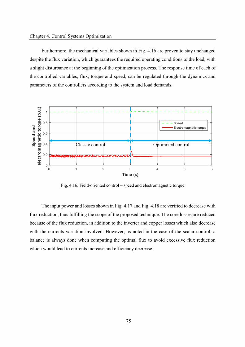
Chapter 4. Control Systems Optimization
75
Furthermore, the mechanical variables shown in Fig. 4.16 are proven to stay unchanged
despite the flux variation, which guarantees the required operating conditions to the load, with
a slight disturbance at the beginning of the optimization process. The response time of each of
the controlled variables, flux, torque and speed, can be regulated through the dynamics and
parameters of the controllers according to the system and load demands.
Fig. 4.16. Field-oriented control – speed and electromagnetic torque
The input power and losses shown in Fig. 4.17 and Fig. 4.18 are verified to decrease with
flux reduction, thus fulfilling the scope of the proposed technique. The core losses are reduced
because of the flux reduction, in addition to the inverter and copper losses which also decrease
with the currents variation involved. However, as noted in the case of the scalar control, a
balance is always done when computing the optimal flux to avoid excessive flux reduction
which would lead to currents increase and efficiency decrease.
Classic control Optimized control
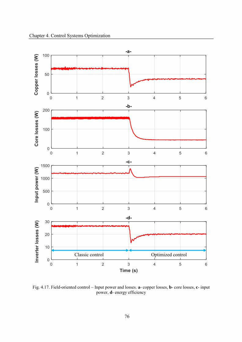
Chapter 4. Control Systems Optimization
76
Fig. 4.17. Field-oriented control – Input power and losses. a- copper losses, b- core losses, c- input power, d- energy efficiency
Classic control Optimized control
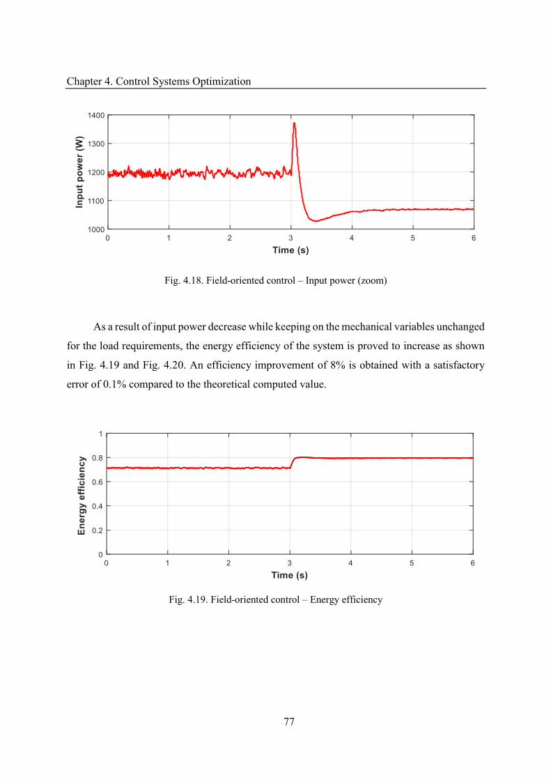
Chapter 4. Control Systems Optimization
77
Fig. 4.18. Field-oriented control – Input power (zoom)
As a result of input power decrease while keeping on the mechanical variables unchanged
for the load requirements, the energy efficiency of the system is proved to increase as shown
in Fig. 4.19 and Fig. 4.20. An efficiency improvement of 8% is obtained with a satisfactory
error of 0.1% compared to the theoretical computed value.
Fig. 4.19. Field-oriented control – Energy efficiency
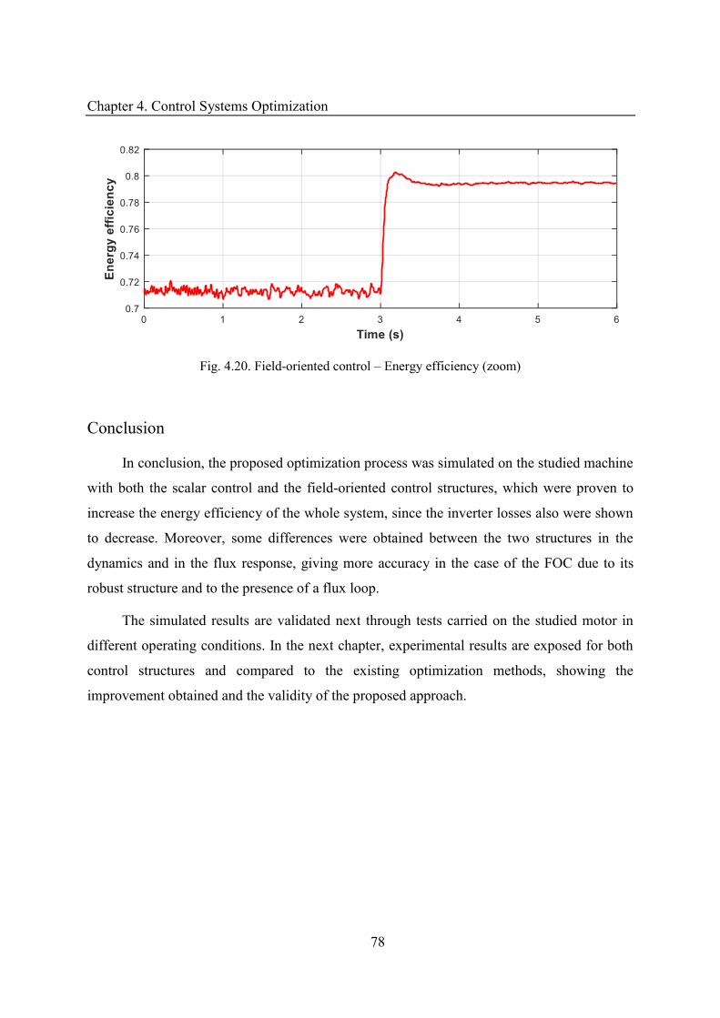
Chapter 4. Control Systems Optimization
78
Fig. 4.20. Field-oriented control – Energy efficiency (zoom)
Conclusion
In conclusion, the proposed optimization process was simulated on the studied machine
with both the scalar control and the field-oriented control structures, which were proven to
increase the energy efficiency of the whole system, since the inverter losses also were shown
to decrease. Moreover, some differences were obtained between the two structures in the
dynamics and in the flux response, giving more accuracy in the case of the FOC due to its
robust structure and to the presence of a flux loop.
The simulated results are validated next through tests carried on the studied motor in
different operating conditions. In the next chapter, experimental results are exposed for both
control structures and compared to the existing optimization methods, showing the
improvement obtained and the validity of the proposed approach.
Chapter 5 Experimental Validations
Table of Contents
Introduction ................................................................................................................ 80
5.1 Experimental Test Bench ............................................................................... 80
5.1.1 Global Test Bench ...................................................................................... 80
5.1.2 Power Elements .......................................................................................... 81
5.1.3 Sensors and Control System ....................................................................... 85
5.1.4 Operating Points Validation ....................................................................... 87
5.2 Optimized Scalar Control Tests ..................................................................... 87
5.2.1 Setup ........................................................................................................... 88
5.2.2 Experimental Results .................................................................................. 89
5.3 Optimized Field-oriented Control Tests ......................................................... 96
5.3.1 Setup ........................................................................................................... 96
5.3.2 Experimental Results .................................................................................. 98
5.4 Comparison with the Existing Optimization Methods ................................. 104
5.4.1 Methods in Literature ............................................................................... 104
5.4.2 Industrial Method ..................................................................................... 106
5.5 IE3 motor tests ............................................................................................. 110
5.5.1 Tested Motor............................................................................................. 110
5.5.2 Experimental Results ................................................................................ 111
5.5.3 Comparison with the IE2 Motor ............................................................... 114
Conclusion ................................................................................................................ 115

Chapter 5. Experimental Validations
80
Introduction
The classic scalar control and field-oriented control were improved through the variation
of flux reference, according to optimal values computed in Chapter 3 aiming to increase the
energy efficiency of the studied system. Simulation results, presented in Chapter 4, showed the
expected improvement along with the decrease of the system losses, especially the core losses.
In the present chapter, experimental results of tests carried on the studied motor with both
optimized control structures are presented. In addition, results of a series of tests with some
existing optimization methods found in literature and industry are presented, to compare their
performances with the proposed method. Finally, the proposed optimization method is tested
on another 5.5kW motor compliant with the IE3 efficiency standard to prove the approach
validity.
5.1 Experimental Test Bench
The experimental test bench used for validation purposes is described in this section in
terms of power elements and all necessary elements for the measurements, signal processing
and control implementation. The tested operating points chosen according to standards used in
industry are also presented.
5.1.1 Global Test Bench
The global experimental test bench built in the LAPLACE laboratory in Toulouse is
constituted of the main elements serving the implementation of the optimized controls and their
appropriate measurements, as shown in Fig. 5.1. The studied IM is fed by an inverter, and the
switches control signals are given by a dSpace controller in which the control structure and
estimators are implemented. A DC generator and resistors serve as the load of the IM, and
suitable currents, voltage and speed sensors are installed to provide the inputs of the control
structure and the estimators. The DC bus of the inverter is provided by an auto-transformer
connected to the grid and a rectifier with suitable capacitors.
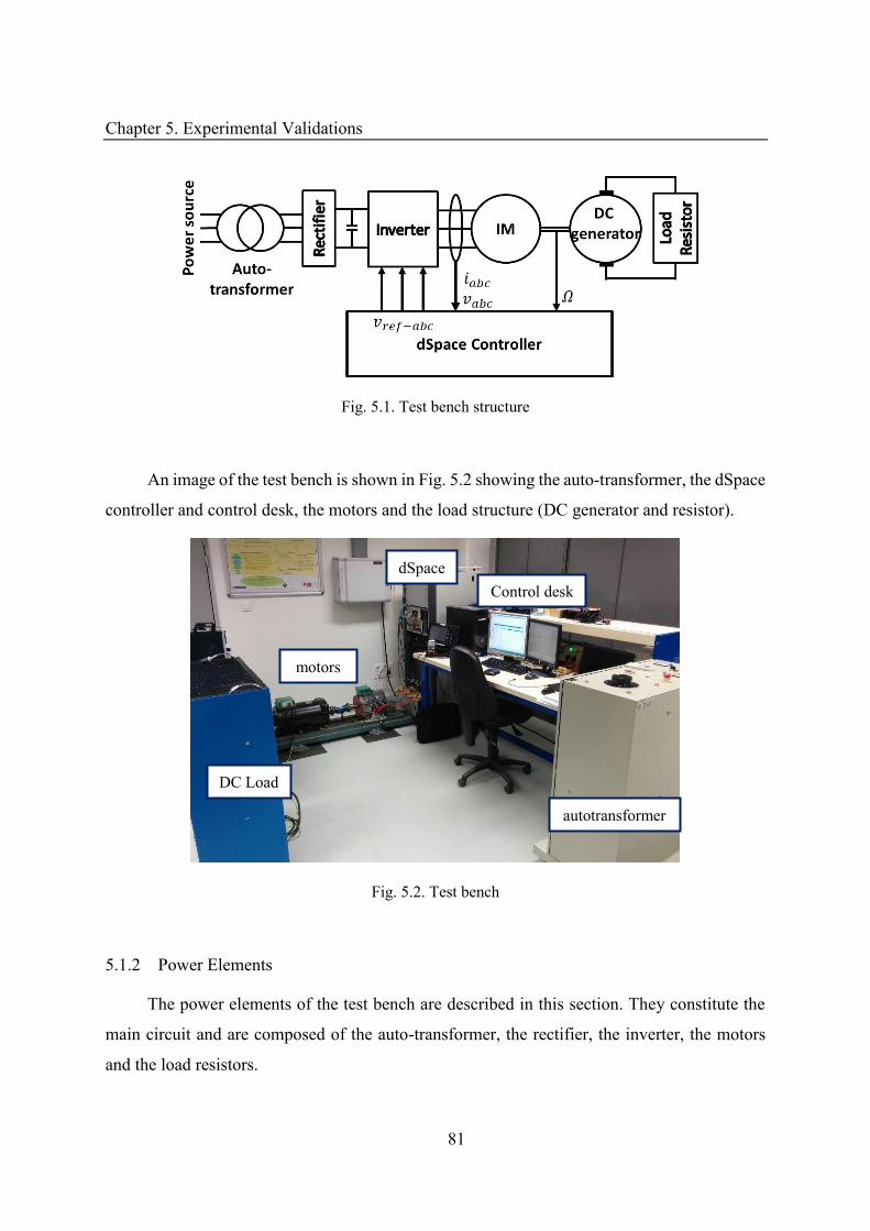
Chapter 5. Experimental Validations
81
Fig. 5.1. Test bench structure
An image of the test bench is shown in Fig. 5.2 showing the auto-transformer, the dSpace
controller and control desk, the motors and the load structure (DC generator and resistor).
Fig. 5.2. Test bench
5.1.2 Power Elements
The power elements of the test bench are described in this section. They constitute the
main circuit and are composed of the auto-transformer, the rectifier, the inverter, the motors
and the load resistors.
autotransformer
Control desk dSpace
motors
DC Load
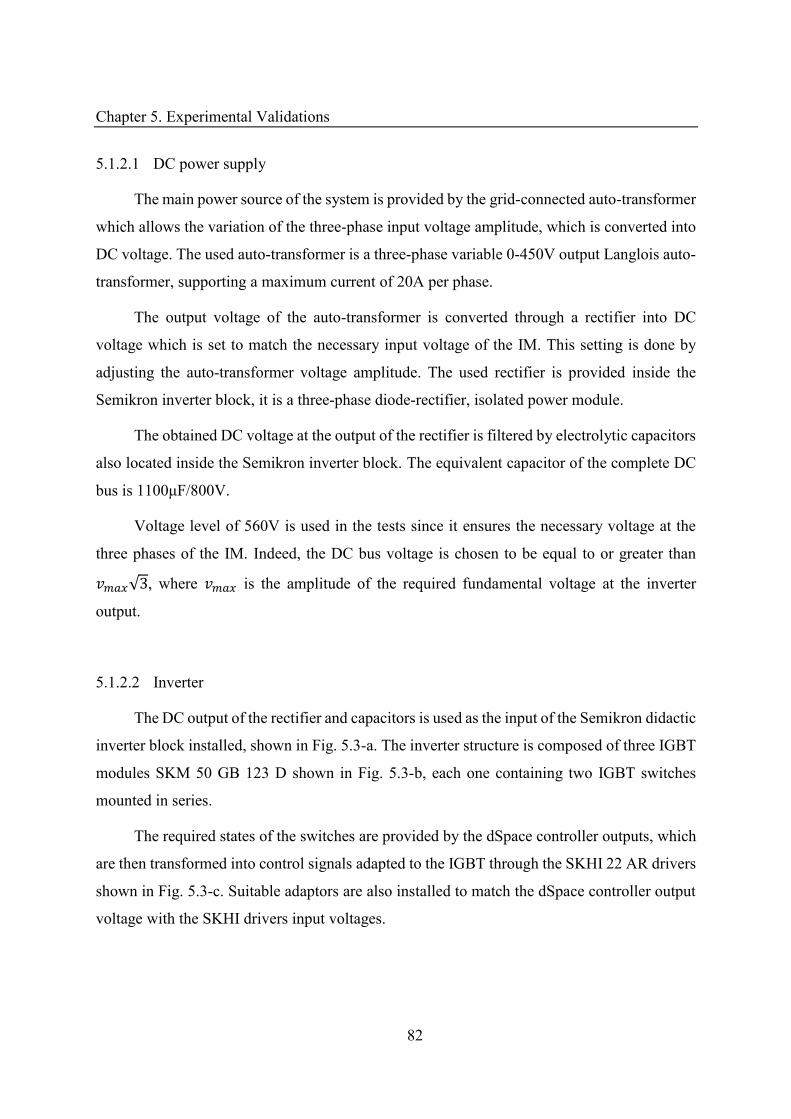
Chapter 5. Experimental Validations
82
5.1.2.1 DC power supply
The main power source of the system is provided by the grid-connected auto-transformer
which allows the variation of the three-phase input voltage amplitude, which is converted into
DC voltage. The used auto-transformer is a three-phase variable 0-450V output Langlois auto-
transformer, supporting a maximum current of 20A per phase.
The output voltage of the auto-transformer is converted through a rectifier into DC
voltage which is set to match the necessary input voltage of the IM. This setting is done by
adjusting the auto-transformer voltage amplitude. The used rectifier is provided inside the
Semikron inverter block, it is a three-phase diode-rectifier, isolated power module.
The obtained DC voltage at the output of the rectifier is filtered by electrolytic capacitors
also located inside the Semikron inverter block. The equivalent capacitor of the complete DC
bus is 1100μF/800V.
Voltage level of 560V is used in the tests since it ensures the necessary voltage at the
three phases of the IM. Indeed, the DC bus voltage is chosen to be equal to or greater than
�√ , where � is the amplitude of the required fundamental voltage at the inverter
output.
5.1.2.2 Inverter
The DC output of the rectifier and capacitors is used as the input of the Semikron didactic
inverter block installed, shown in Fig. 5.3-a. The inverter structure is composed of three IGBT
modules SKM 50 GB 123 D shown in Fig. 5.3-b, each one containing two IGBT switches
mounted in series.
The required states of the switches are provided by the dSpace controller outputs, which
are then transformed into control signals adapted to the IGBT through the SKHI 22 AR drivers
shown in Fig. 5.3-c. Suitable adaptors are also installed to match the dSpace controller output
voltage with the SKHI drivers input voltages.
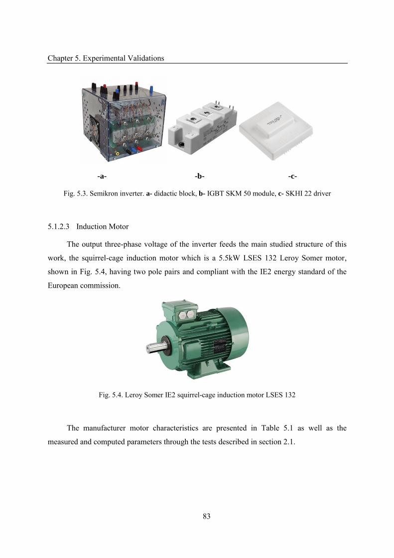
Chapter 5. Experimental Validations
83
-a- -b- -c-
Fig. 5.3. Semikron inverter. a- didactic block, b- IGBT SKM 50 module, c- SKHI 22 driver
5.1.2.3 Induction Motor
The output three-phase voltage of the inverter feeds the main studied structure of this
work, the squirrel-cage induction motor which is a 5.5kW LSES 132 Leroy Somer motor,
shown in Fig. 5.4, having two pole pairs and compliant with the IE2 energy standard of the
European commission.
Fig. 5.4. Leroy Somer IE2 squirrel-cage induction motor LSES 132
The manufacturer motor characteristics are presented in Table 5.1 as well as the
measured and computed parameters through the tests described in section 2.1.
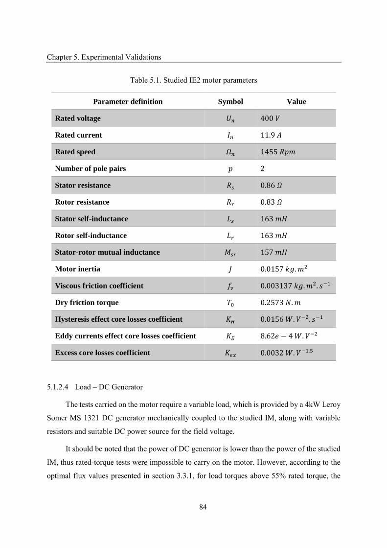
Chapter 5. Experimental Validations
84
Table 5.1. Studied IE2 motor parameters
Parameter definition Symbol Value
Rated voltage
Rated current .
Rated speed �
Number of pole pairs
Stator resistance . �
Rotor resistance . �
Stator self-inductance
Rotor self-inductance
Stator-rotor mutual inductance
Motor inertia . .
Viscous friction coefficient � . . . −
Dry friction torque . .
Hysteresis effect core losses coefficient � . . − . −
Eddy currents effect core losses coefficient . − . −
Excess core losses coefficient � . . − .5
5.1.2.4 Load – DC Generator
The tests carried on the motor require a variable load, which is provided by a 4kW Leroy
Somer MS 1321 DC generator mechanically coupled to the studied IM, along with variable
resistors and suitable DC power source for the field voltage.
It should be noted that the power of DC generator is lower than the power of the studied
IM, thus rated-torque tests were impossible to carry on the motor. However, according to the
optimal flux values presented in section 3.3.1, for load torques above 55% rated torque, the
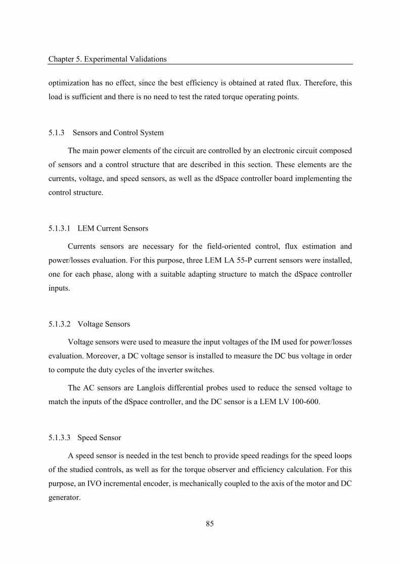
Chapter 5. Experimental Validations
85
optimization has no effect, since the best efficiency is obtained at rated flux. Therefore, this
load is sufficient and there is no need to test the rated torque operating points.
5.1.3 Sensors and Control System
The main power elements of the circuit are controlled by an electronic circuit composed
of sensors and a control structure that are described in this section. These elements are the
currents, voltage, and speed sensors, as well as the dSpace controller board implementing the
control structure.
5.1.3.1 LEM Current Sensors
Currents sensors are necessary for the field-oriented control, flux estimation and
power/losses evaluation. For this purpose, three LEM LA 55-P current sensors were installed,
one for each phase, along with a suitable adapting structure to match the dSpace controller
inputs.
5.1.3.2 Voltage Sensors
Voltage sensors were used to measure the input voltages of the IM used for power/losses
evaluation. Moreover, a DC voltage sensor is installed to measure the DC bus voltage in order
to compute the duty cycles of the inverter switches.
The AC sensors are Langlois differential probes used to reduce the sensed voltage to
match the inputs of the dSpace controller, and the DC sensor is a LEM LV 100-600.
5.1.3.3 Speed Sensor
A speed sensor is needed in the test bench to provide speed readings for the speed loops
of the studied controls, as well as for the torque observer and efficiency calculation. For this
purpose, an IVO incremental encoder, is mechanically coupled to the axis of the motor and DC
generator.
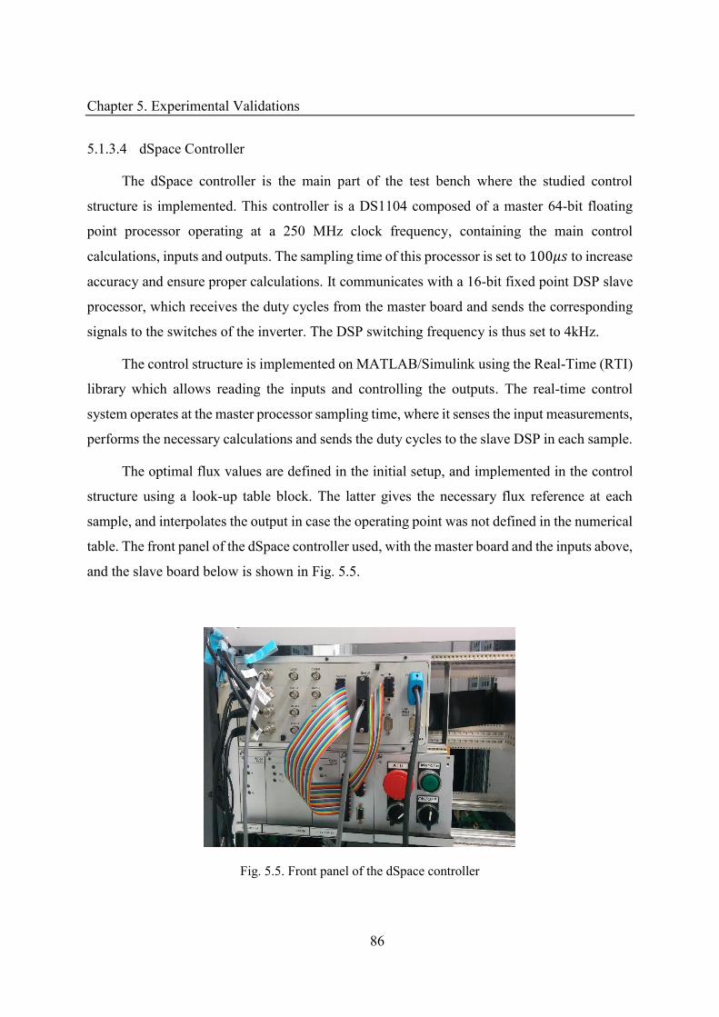
Chapter 5. Experimental Validations
86
5.1.3.4 dSpace Controller
The dSpace controller is the main part of the test bench where the studied control
structure is implemented. This controller is a DS1104 composed of a master 64-bit floating
point processor operating at a 250 MHz clock frequency, containing the main control
calculations, inputs and outputs. The sampling time of this processor is set to � to increase
accuracy and ensure proper calculations. It communicates with a 16-bit fixed point DSP slave
processor, which receives the duty cycles from the master board and sends the corresponding
signals to the switches of the inverter. The DSP switching frequency is thus set to 4kHz.
The control structure is implemented on MATLAB/Simulink using the Real-Time (RTI)
library which allows reading the inputs and controlling the outputs. The real-time control
system operates at the master processor sampling time, where it senses the input measurements,
performs the necessary calculations and sends the duty cycles to the slave DSP in each sample.
The optimal flux values are defined in the initial setup, and implemented in the control
structure using a look-up table block. The latter gives the necessary flux reference at each
sample, and interpolates the output in case the operating point was not defined in the numerical
table. The front panel of the dSpace controller used, with the master board and the inputs above,
and the slave board below is shown in Fig. 5.5.
Fig. 5.5. Front panel of the dSpace controller
Chapter 5. Experimental Validations
87
5.1.4 Operating Points Validation
The constructed test bench can serve for several operating points below the rated values
of the elements included. However, specific points are chosen by motor manufacturers like
Leroy-Somer according to standard IEC 60034-30-2 [95], thus defining a range of operating
conditions in terms of speed and load torque to be validated, as presented in Fig. 5.6-a.
Consequently, the following experimental results will be presented according to these
points, in addition to some others, as shown in Fig. 5.6-b, for a better analysis of the
optimization effect. However, the rated torque points are not reached as noted in 5.1.2.4
because of the low rated power of the DC generator.
-a- -b-
Fig. 5.6. Experimental validation operating points. a- industrial test points, b- effective test points
5.2 Optimized Scalar Control Tests
The described test bench is used to test the optimized scalar control detailed in section
4.1 and validate the simulation results obtained. The setup of the control system and its
experimental results are presented in this section.
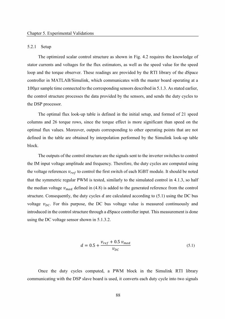
Chapter 5. Experimental Validations
88
5.2.1 Setup
The optimized scalar control structure as shown in Fig. 4.2 requires the knowledge of
stator currents and voltages for the flux estimators, as well as the speed value for the speed
loop and the torque observer. These readings are provided by the RTI library of the dSpace
controller in MATLAB/Simulink, which communicates with the master board operating at a � sample time connected to the corresponding sensors described in 5.1.3. As stated earlier,
the control structure processes the data provided by the sensors, and sends the duty cycles to
the DSP processor.
The optimal flux look-up table is defined in the initial setup, and formed of 21 speed
columns and 26 torque rows, since the torque effect is more significant than speed on the
optimal flux values. Moreover, outputs corresponding to other operating points that are not
defined in the table are obtained by interpolation performed by the Simulink look-up table
block.
The outputs of the control structure are the signals sent to the inverter switches to control
the IM input voltage amplitude and frequency. Therefore, the duty cycles are computed using
the voltage references to control the first switch of each IGBT module. It should be noted
that the symmetric regular PWM is tested, similarly to the simulated control in 4.1.3, so half
the median voltage defined in (4.8) is added to the generated reference from the control
structure. Consequently, the duty cycles are calculated according to (5.1) using the DC bus
voltage . For this purpose, the DC bus voltage value is measured continuously and
introduced in the control structure through a dSpace controller input. This measurement is done
using the DC voltage sensor shown in 5.1.3.2.
= . + + . (5.1)
Once the duty cycles computed, a PWM block in the Simulink RTI library
communicating with the DSP slave board is used, it converts each duty cycle into two signals
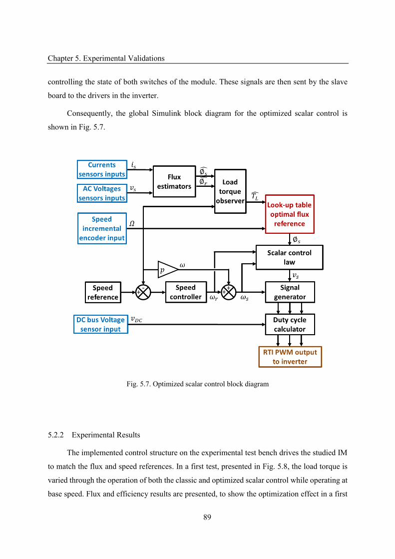
Chapter 5. Experimental Validations
89
controlling the state of both switches of the module. These signals are then sent by the slave
board to the drivers in the inverter.
Consequently, the global Simulink block diagram for the optimized scalar control is
shown in Fig. 5.7.
Fig. 5.7. Optimized scalar control block diagram
5.2.2 Experimental Results
The implemented control structure on the experimental test bench drives the studied IM
to match the flux and speed references. In a first test, presented in Fig. 5.8, the load torque is
varied through the operation of both the classic and optimized scalar control while operating at
base speed. Flux and efficiency results are presented, to show the optimization effect in a first
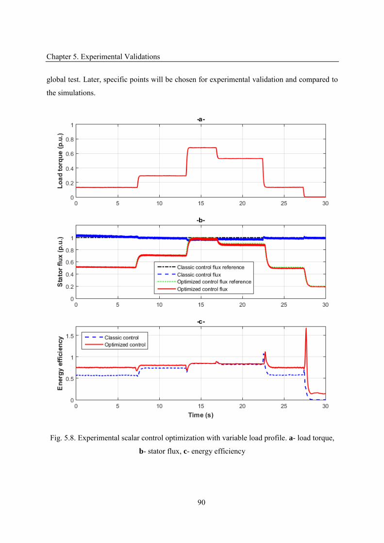
Chapter 5. Experimental Validations
90
global test. Later, specific points will be chosen for experimental validation and compared to
the simulations.
Fig. 5.8. Experimental scalar control optimization with variable load profile. a- load torque,
b- stator flux, c- energy efficiency
Chapter 5. Experimental Validations
91
Results show that the optimized control adapts the stator flux with the load torque, thus,
the efficiency is optimized compared to the case of the classic scalar control. It should be noted
that the high transient efficiency values (above 1) are due to the lack of robustness of the scalar
control in transient phases, which causes oscillations of the dynamic variables in the case of
important torque gradients, especially with low loads. Results also show that for torque values
that exceed 0.55p.u., the flux reference in both controls is equal to the rated flux, hence no
optimization is observed.
On the other hand, tests were performed for a series of operating points, defined in 5.1.4,
however, since the results are similar for all points with some differences in the efficiency
improvement, the presented results correspond to an operation at 0.5p.u. speed and 0.25p.u.
torque. This choice corresponds to a low torque operating point, where the optimization is
effective, as stated in section 3.3.1.
Furthermore, as detailed in section 4.1.2, to ensure a proper start-up of the motor, rated
flux is established first, then the control optimization is launched to set the optimal stator flux
and improve the efficiency. In the results shown, the steady-state is already established at time
t=0s, then at t=3s, the optimization procedure is applied to show the difference with the
classical scalar control performances. Simulation and experimental results are presented on the
same figures for validation.
First, the optimization process in terms of stator flux reference is presented in Fig. 5.9-a
showing the decrease at t=3s to meet the optimized value defined in the look-up table according
to the measured speed and estimated load torque. Simultaneously, a slight distortion in the
speed curve and the electromagnetic torque is observed to cope with the flux variation, as it
can be seen in Fig. 5.9-b, then the steady-state is established again.
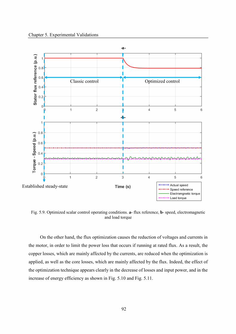
Chapter 5. Experimental Validations
92
Fig. 5.9. Optimized scalar control operating conditions. a- flux reference, b- speed, electromagnetic and load torque
On the other hand, the flux optimization causes the reduction of voltages and currents in
the motor, in order to limit the power loss that occurs if running at rated flux. As a result, the
copper losses, which are mainly affected by the currents, are reduced when the optimization is
applied, as well as the core losses, which are mainly affected by the flux. Indeed, the effect of
the optimization technique appears clearly in the decrease of losses and input power, and in the
increase of energy efficiency as shown in Fig. 5.10 and Fig. 5.11.
Classic control Optimized control
Established steady-state
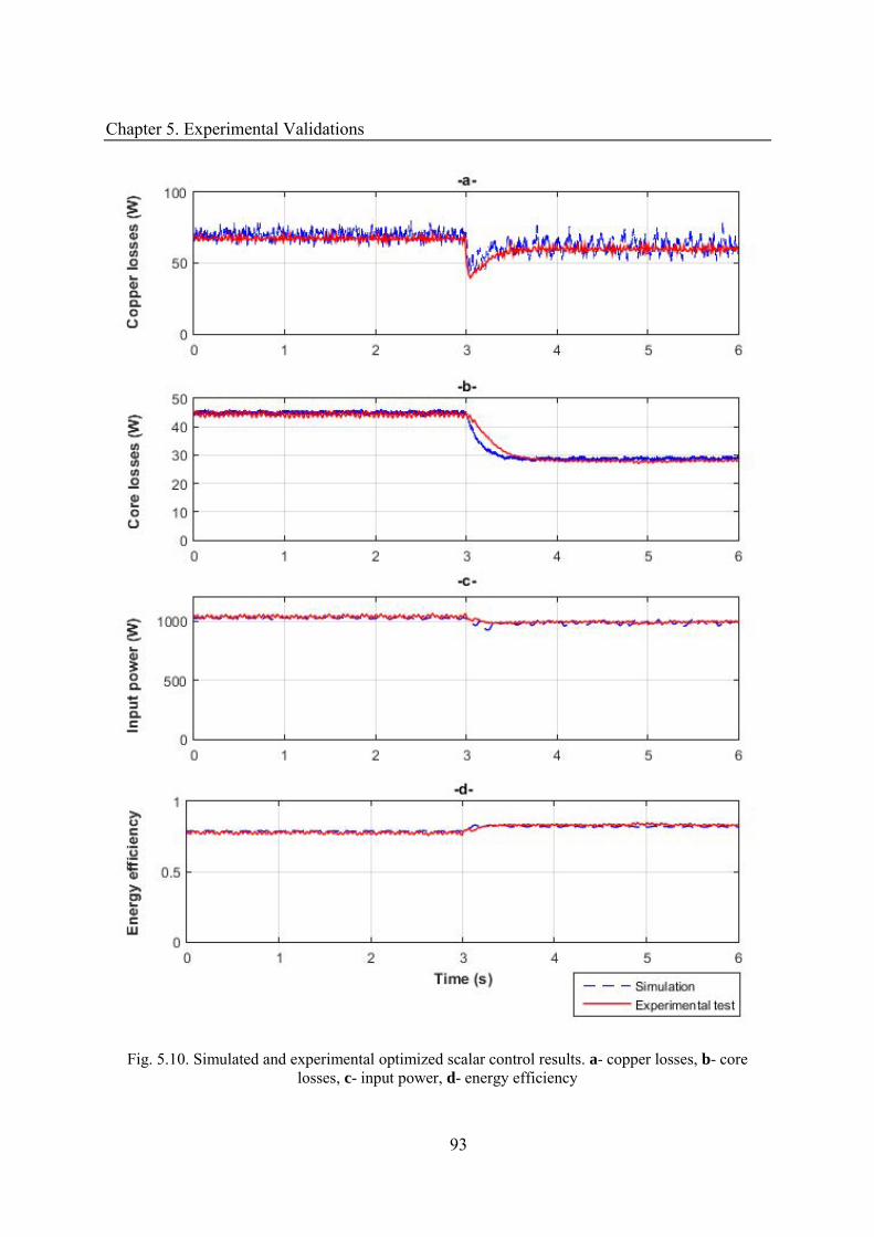
Chapter 5. Experimental Validations
93
Fig. 5.10. Simulated and experimental optimized scalar control results. a- copper losses, b- core losses, c- input power, d- energy efficiency
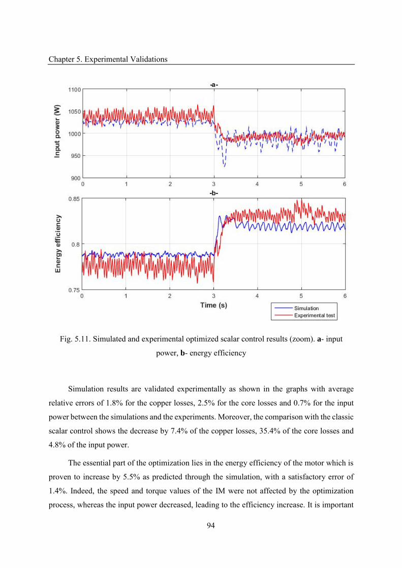
Chapter 5. Experimental Validations
94
Fig. 5.11. Simulated and experimental optimized scalar control results (zoom). a- input
power, b- energy efficiency
Simulation results are validated experimentally as shown in the graphs with average
relative errors of 1.8% for the copper losses, 2.5% for the core losses and 0.7% for the input
power between the simulations and the experiments. Moreover, the comparison with the classic
scalar control shows the decrease by 7.4% of the copper losses, 35.4% of the core losses and
4.8% of the input power.
The essential part of the optimization lies in the energy efficiency of the motor which is
proven to increase by 5.5% as predicted through the simulation, with a satisfactory error of
1.4%. Indeed, the speed and torque values of the IM were not affected by the optimization
process, whereas the input power decreased, leading to the efficiency increase. It is important
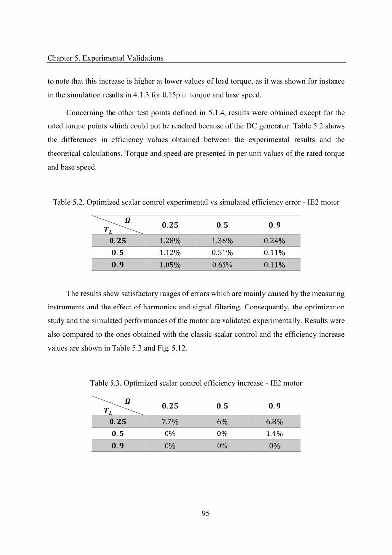
Chapter 5. Experimental Validations
95
to note that this increase is higher at lower values of load torque, as it was shown for instance
in the simulation results in 4.1.3 for 0.15p.u. torque and base speed.
Concerning the other test points defined in 5.1.4, results were obtained except for the
rated torque points which could not be reached because of the DC generator. Table 5.2 shows
the differences in efficiency values obtained between the experimental results and the
theoretical calculations. Torque and speed are presented in per unit values of the rated torque
and base speed.
Table 5.2. Optimized scalar control experimental vs simulated efficiency error - IE2 motor � �� . . . . . % . % . % . . % . % . % . . % 0.65% . %
The results show satisfactory ranges of errors which are mainly caused by the measuring
instruments and the effect of harmonics and signal filtering. Consequently, the optimization
study and the simulated performances of the motor are validated experimentally. Results were
also compared to the ones obtained with the classic scalar control and the efficiency increase
values are shown in Table 5.3 and Fig. 5.12.
Table 5.3. Optimized scalar control efficiency increase - IE2 motor � �� . . . . . % % . % . % % . % . % 0% %
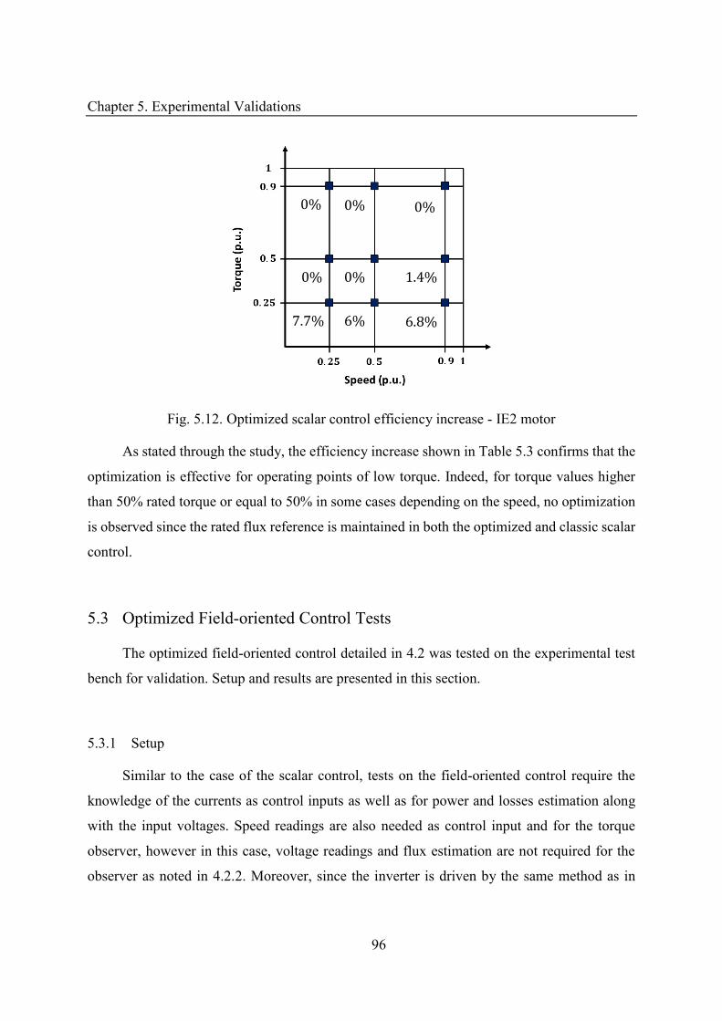
Chapter 5. Experimental Validations
96
Fig. 5.12. Optimized scalar control efficiency increase - IE2 motor
As stated through the study, the efficiency increase shown in Table 5.3 confirms that the
optimization is effective for operating points of low torque. Indeed, for torque values higher
than 50% rated torque or equal to 50% in some cases depending on the speed, no optimization
is observed since the rated flux reference is maintained in both the optimized and classic scalar
control.
5.3 Optimized Field-oriented Control Tests
The optimized field-oriented control detailed in 4.2 was tested on the experimental test
bench for validation. Setup and results are presented in this section.
5.3.1 Setup
Similar to the case of the scalar control, tests on the field-oriented control require the
knowledge of the currents as control inputs as well as for power and losses estimation along
with the input voltages. Speed readings are also needed as control input and for the torque
observer, however in this case, voltage readings and flux estimation are not required for the
observer as noted in 4.2.2. Moreover, since the inverter is driven by the same method as in
% % %
% . %
. % %
%
. %
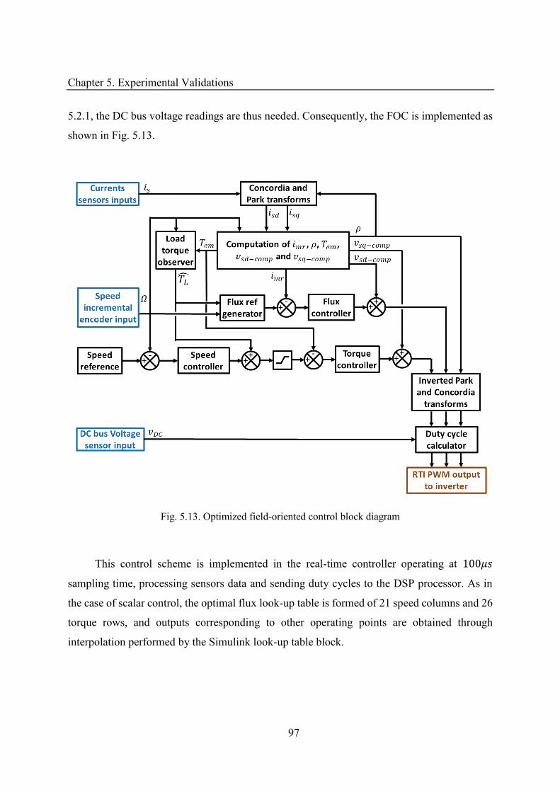
Chapter 5. Experimental Validations
97
5.2.1, the DC bus voltage readings are thus needed. Consequently, the FOC is implemented as
shown in Fig. 5.13.
Fig. 5.13. Optimized field-oriented control block diagram
This control scheme is implemented in the real-time controller operating at �
sampling time, processing sensors data and sending duty cycles to the DSP processor. As in
the case of scalar control, the optimal flux look-up table is formed of 21 speed columns and 26
torque rows, and outputs corresponding to other operating points are obtained through
interpolation performed by the Simulink look-up table block.
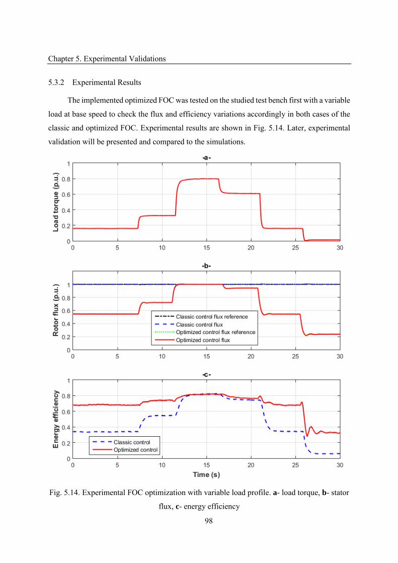
Chapter 5. Experimental Validations
98
5.3.2 Experimental Results
The implemented optimized FOC was tested on the studied test bench first with a variable
load at base speed to check the flux and efficiency variations accordingly in both cases of the
classic and optimized FOC. Experimental results are shown in Fig. 5.14. Later, experimental
validation will be presented and compared to the simulations.
Fig. 5.14. Experimental FOC optimization with variable load profile. a- load torque, b- stator
flux, c- energy efficiency
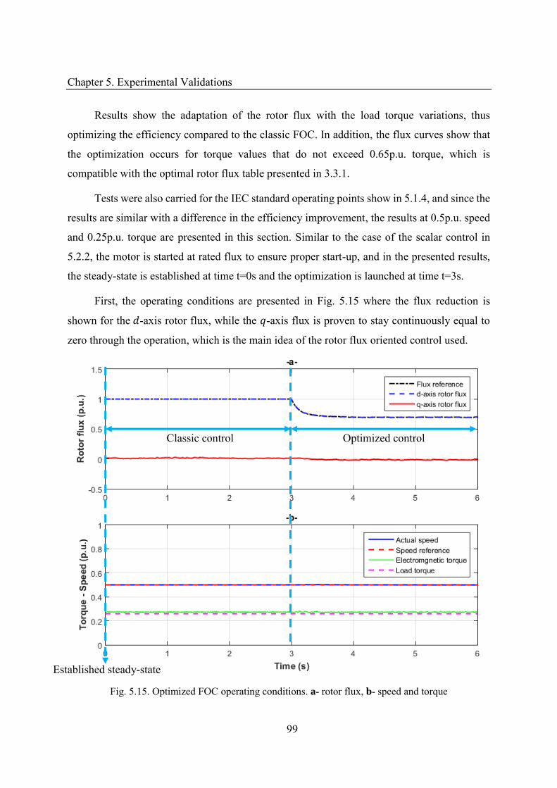
Chapter 5. Experimental Validations
99
Results show the adaptation of the rotor flux with the load torque variations, thus
optimizing the efficiency compared to the classic FOC. In addition, the flux curves show that
the optimization occurs for torque values that do not exceed 0.65p.u. torque, which is
compatible with the optimal rotor flux table presented in 3.3.1.
Tests were also carried for the IEC standard operating points show in 5.1.4, and since the
results are similar with a difference in the efficiency improvement, the results at 0.5p.u. speed
and 0.25p.u. torque are presented in this section. Similar to the case of the scalar control in
5.2.2, the motor is started at rated flux to ensure proper start-up, and in the presented results,
the steady-state is established at time t=0s and the optimization is launched at time t=3s.
First, the operating conditions are presented in Fig. 5.15 where the flux reduction is
shown for the -axis rotor flux, while the -axis flux is proven to stay continuously equal to
zero through the operation, which is the main idea of the rotor flux oriented control used.
Fig. 5.15. Optimized FOC operating conditions. a- rotor flux, b- speed and torque
Classic control Optimized control
Established steady-state
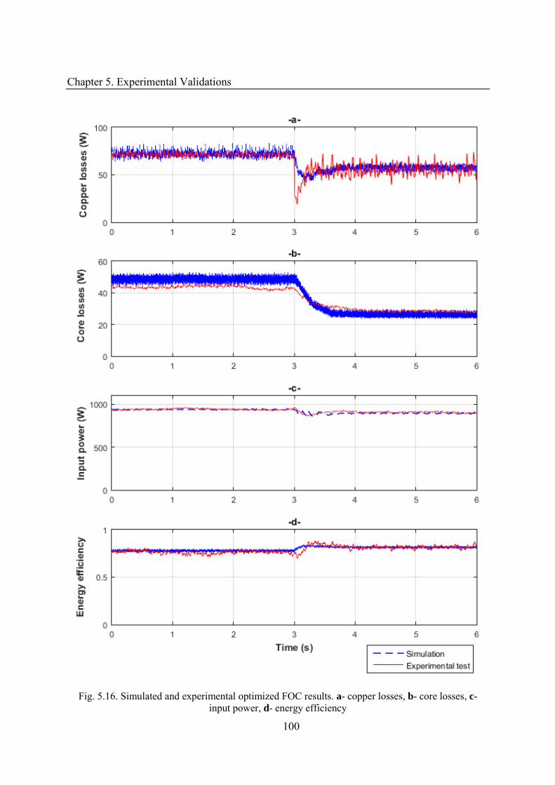
Chapter 5. Experimental Validations
100
Fig. 5.16. Simulated and experimental optimized FOC results. a- copper losses, b- core losses, c- input power, d- energy efficiency
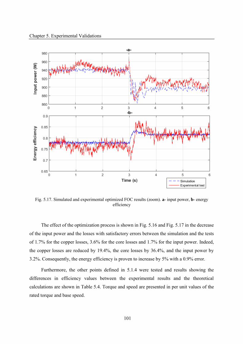
Chapter 5. Experimental Validations
101
Fig. 5.17. Simulated and experimental optimized FOC results (zoom). a- input power, b- energy efficiency
The effect of the optimization process is shown in Fig. 5.16 and Fig. 5.17 in the decrease
of the input power and the losses with satisfactory errors between the simulation and the tests
of 1.7% for the copper losses, 3.6% for the core losses and 1.7% for the input power. Indeed,
the copper losses are reduced by 19.4%, the core losses by 36.4%, and the input power by
3.2%. Consequently, the energy efficiency is proven to increase by 5% with a 0.9% error.
Furthermore, the other points defined in 5.1.4 were tested and results showing the
differences in efficiency values between the experimental results and the theoretical
calculations are shown in Table 5.4. Torque and speed are presented in per unit values of the
rated torque and base speed.
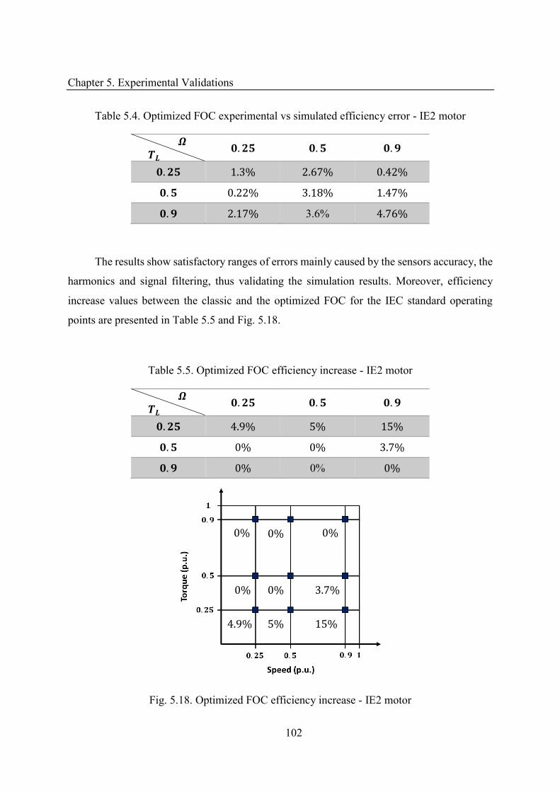
Chapter 5. Experimental Validations
102
Table 5.4. Optimized FOC experimental vs simulated efficiency error - IE2 motor � �� . . . . . % . % . % . . % . % . % . . % 3.6% . %
The results show satisfactory ranges of errors mainly caused by the sensors accuracy, the
harmonics and signal filtering, thus validating the simulation results. Moreover, efficiency
increase values between the classic and the optimized FOC for the IEC standard operating
points are presented in Table 5.5 and Fig. 5.18.
Table 5.5. Optimized FOC efficiency increase - IE2 motor � �� . . . . . % % % . % % . % . % 0% %
Fig. 5.18. Optimized FOC efficiency increase - IE2 motor
% % %
% . %
. % %
%
%
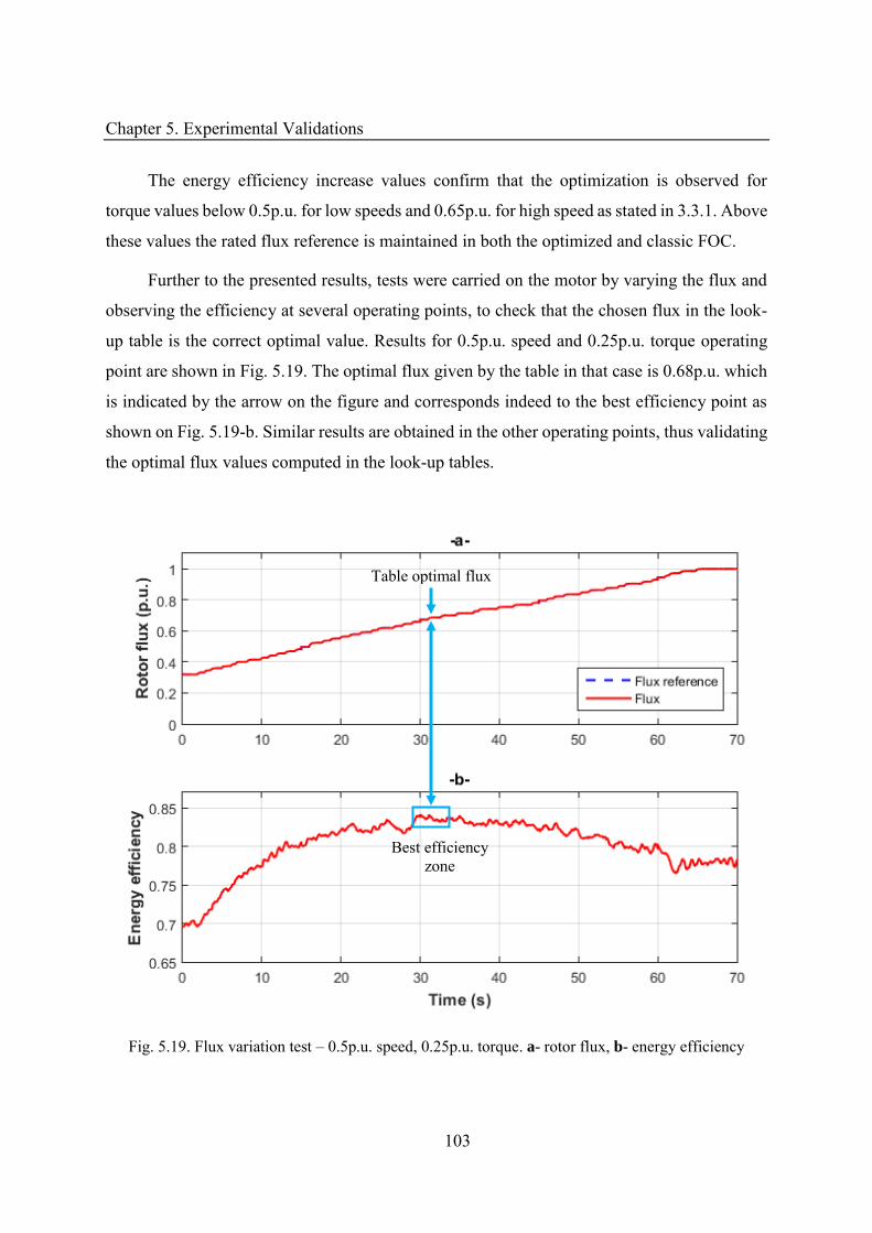
Chapter 5. Experimental Validations
103
The energy efficiency increase values confirm that the optimization is observed for
torque values below 0.5p.u. for low speeds and 0.65p.u. for high speed as stated in 3.3.1. Above
these values the rated flux reference is maintained in both the optimized and classic FOC.
Further to the presented results, tests were carried on the motor by varying the flux and
observing the efficiency at several operating points, to check that the chosen flux in the look-
up table is the correct optimal value. Results for 0.5p.u. speed and 0.25p.u. torque operating
point are shown in Fig. 5.19. The optimal flux given by the table in that case is 0.68p.u. which
is indicated by the arrow on the figure and corresponds indeed to the best efficiency point as
shown on Fig. 5.19-b. Similar results are obtained in the other operating points, thus validating
the optimal flux values computed in the look-up tables.
Fig. 5.19. Flux variation test – 0.5p.u. speed, 0.25p.u. torque. a- rotor flux, b- energy efficiency
Table optimal flux
Best efficiency zone
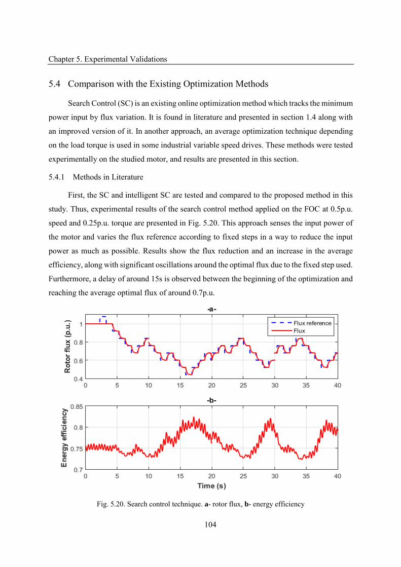
Chapter 5. Experimental Validations
104
5.4 Comparison with the Existing Optimization Methods
Search Control (SC) is an existing online optimization method which tracks the minimum
power input by flux variation. It is found in literature and presented in section 1.4 along with
an improved version of it. In another approach, an average optimization technique depending
on the load torque is used in some industrial variable speed drives. These methods were tested
experimentally on the studied motor, and results are presented in this section.
5.4.1 Methods in Literature
First, the SC and intelligent SC are tested and compared to the proposed method in this
study. Thus, experimental results of the search control method applied on the FOC at 0.5p.u.
speed and 0.25p.u. torque are presented in Fig. 5.20. This approach senses the input power of
the motor and varies the flux reference according to fixed steps in a way to reduce the input
power as much as possible. Results show the flux reduction and an increase in the average
efficiency, along with significant oscillations around the optimal flux due to the fixed step used.
Furthermore, a delay of around 15s is observed between the beginning of the optimization and
reaching the average optimal flux of around 0.7p.u.
Fig. 5.20. Search control technique. a- rotor flux, b- energy efficiency
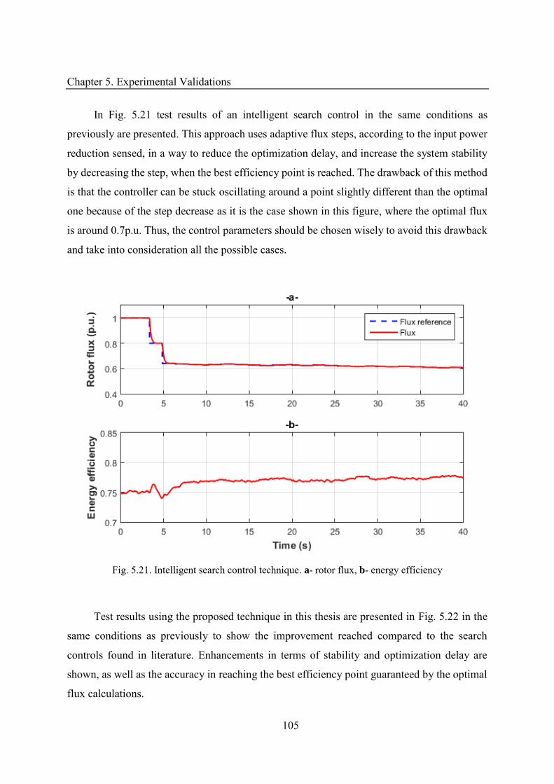
Chapter 5. Experimental Validations
105
In Fig. 5.21 test results of an intelligent search control in the same conditions as
previously are presented. This approach uses adaptive flux steps, according to the input power
reduction sensed, in a way to reduce the optimization delay, and increase the system stability
by decreasing the step, when the best efficiency point is reached. The drawback of this method
is that the controller can be stuck oscillating around a point slightly different than the optimal
one because of the step decrease as it is the case shown in this figure, where the optimal flux
is around 0.7p.u. Thus, the control parameters should be chosen wisely to avoid this drawback
and take into consideration all the possible cases.
Fig. 5.21. Intelligent search control technique. a- rotor flux, b- energy efficiency
Test results using the proposed technique in this thesis are presented in Fig. 5.22 in the
same conditions as previously to show the improvement reached compared to the search
controls found in literature. Enhancements in terms of stability and optimization delay are
shown, as well as the accuracy in reaching the best efficiency point guaranteed by the optimal
flux calculations.
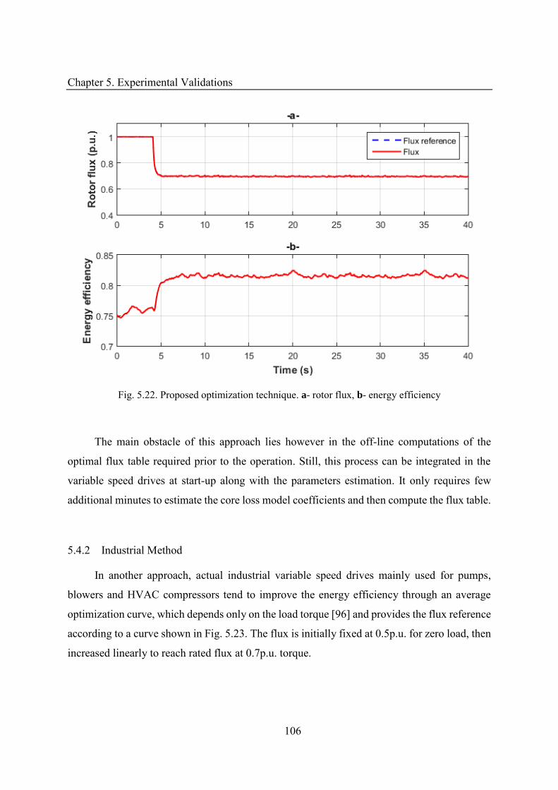
Chapter 5. Experimental Validations
106
Fig. 5.22. Proposed optimization technique. a- rotor flux, b- energy efficiency
The main obstacle of this approach lies however in the off-line computations of the
optimal flux table required prior to the operation. Still, this process can be integrated in the
variable speed drives at start-up along with the parameters estimation. It only requires few
additional minutes to estimate the core loss model coefficients and then compute the flux table.
5.4.2 Industrial Method
In another approach, actual industrial variable speed drives mainly used for pumps,
blowers and HVAC compressors tend to improve the energy efficiency through an average
optimization curve, which depends only on the load torque [96] and provides the flux reference
according to a curve shown in Fig. 5.23. The flux is initially fixed at 0.5p.u. for zero load, then
increased linearly to reach rated flux at 0.7p.u. torque.
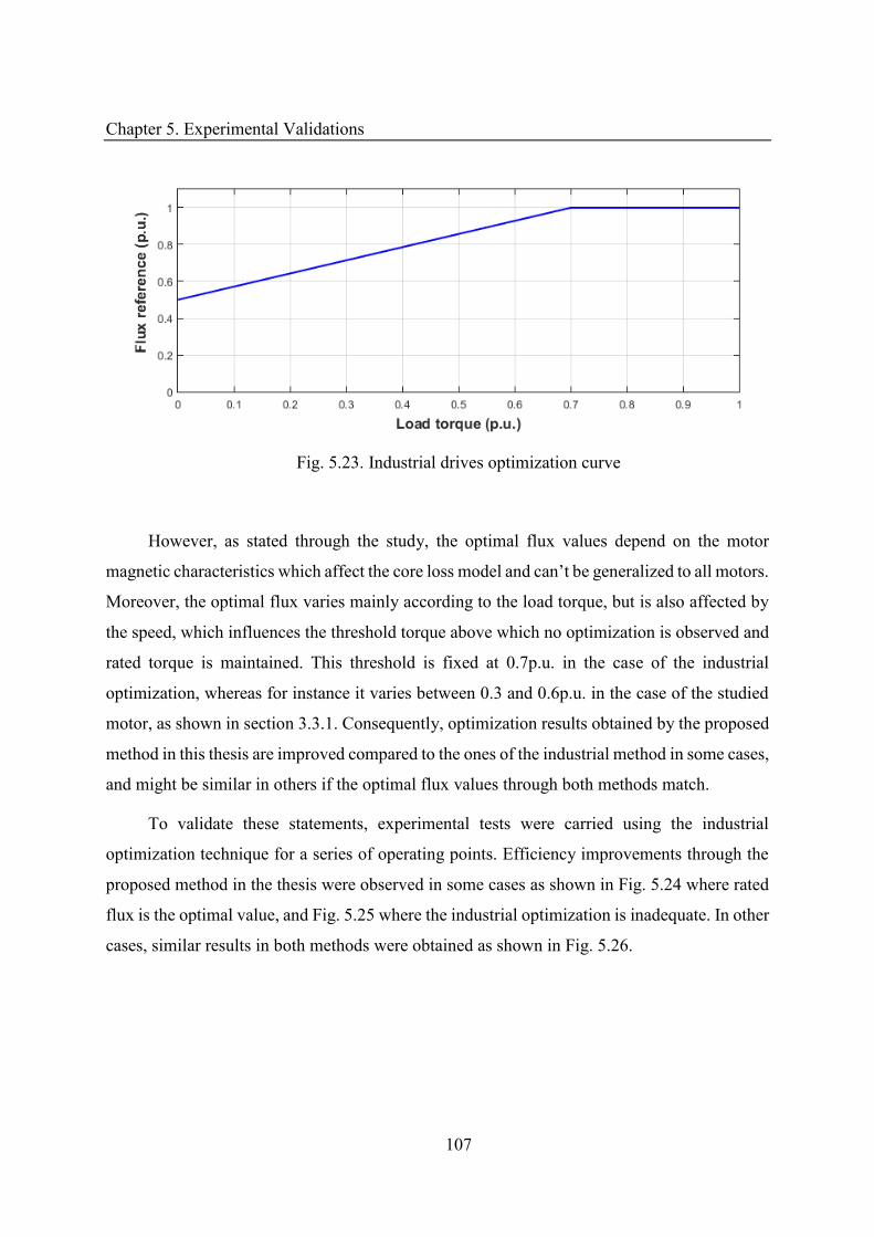
Chapter 5. Experimental Validations
107
Fig. 5.23. Industrial drives optimization curve
However, as stated through the study, the optimal flux values depend on the motor
magnetic characteristics which affect the core loss model and can’t be generalized to all motors.
Moreover, the optimal flux varies mainly according to the load torque, but is also affected by
the speed, which influences the threshold torque above which no optimization is observed and
rated torque is maintained. This threshold is fixed at 0.7p.u. in the case of the industrial
optimization, whereas for instance it varies between 0.3 and 0.6p.u. in the case of the studied
motor, as shown in section 3.3.1. Consequently, optimization results obtained by the proposed
method in this thesis are improved compared to the ones of the industrial method in some cases,
and might be similar in others if the optimal flux values through both methods match.
To validate these statements, experimental tests were carried using the industrial
optimization technique for a series of operating points. Efficiency improvements through the
proposed method in the thesis were observed in some cases as shown in Fig. 5.24 where rated
flux is the optimal value, and Fig. 5.25 where the industrial optimization is inadequate. In other
cases, similar results in both methods were obtained as shown in Fig. 5.26.
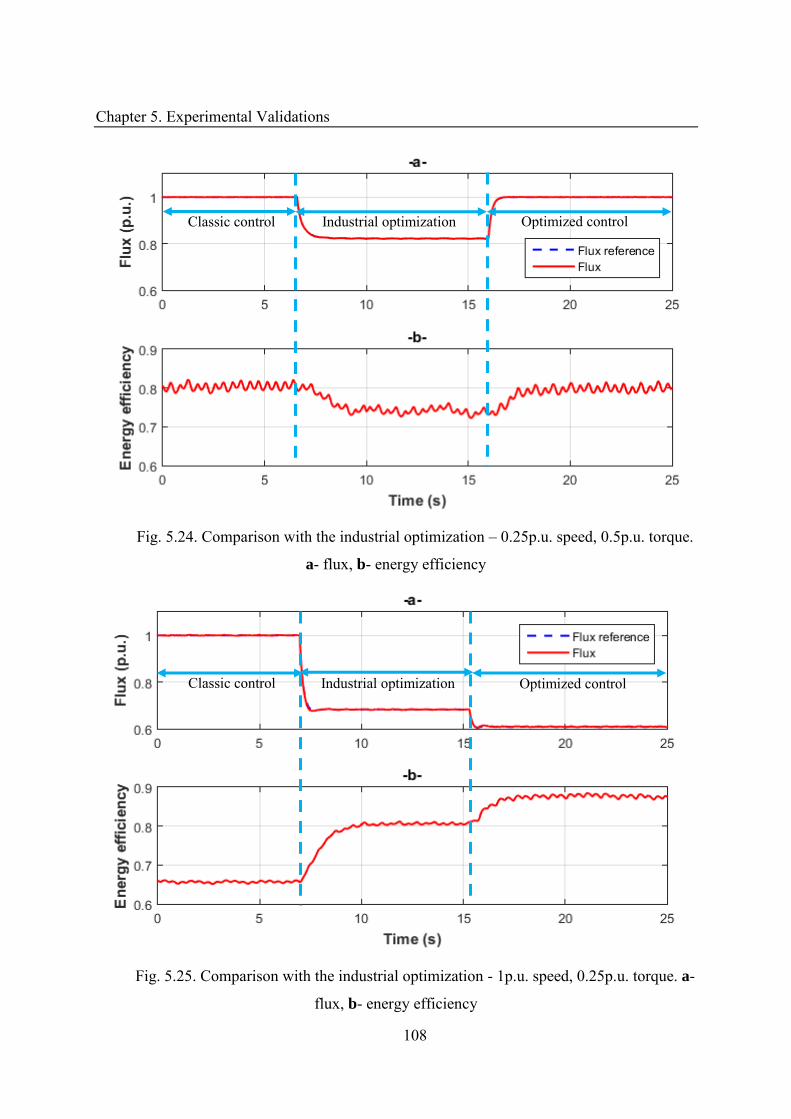
Chapter 5. Experimental Validations
108
Fig. 5.24. Comparison with the industrial optimization – 0.25p.u. speed, 0.5p.u. torque.
a- flux, b- energy efficiency
Fig. 5.25. Comparison with the industrial optimization - 1p.u. speed, 0.25p.u. torque. a-
flux, b- energy efficiency
Classic control Industrial optimization Optimized control
Classic control Industrial optimization Optimized control
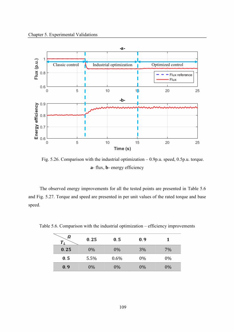
Chapter 5. Experimental Validations
109
Fig. 5.26. Comparison with the industrial optimization – 0.9p.u. speed, 0.5p.u. torque.
a- flux, b- energy efficiency
The observed energy improvements for all the tested points are presented in Table 5.6
and Fig. 5.27. Torque and speed are presented in per unit values of the rated torque and base
speed.
Table 5.6. Comparison with the industrial optimization – efficiency improvements � �� . . . . % % % % . . % . % % % . % % % %
Classic control Industrial optimization Optimized control
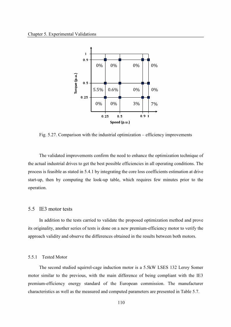
Chapter 5. Experimental Validations
110
Fig. 5.27. Comparison with the industrial optimization – efficiency improvements
The validated improvements confirm the need to enhance the optimization technique of
the actual industrial drives to get the best possible efficiencies in all operating conditions. The
process is feasible as stated in 5.4.1 by integrating the core loss coefficients estimation at drive
start-up, then by computing the look-up table, which requires few minutes prior to the
operation.
5.5 IE3 motor tests
In addition to the tests carried to validate the proposed optimization method and prove
its originality, another series of tests is done on a new premium-efficiency motor to verify the
approach validity and observe the differences obtained in the results between both motors.
5.5.1 Tested Motor
The second studied squirrel-cage induction motor is a 5.5kW LSES 132 Leroy Somer
motor similar to the previous, with the main difference of being compliant with the IE3
premium-efficiency energy standard of the European commission. The manufacturer
characteristics as well as the measured and computed parameters are presented in Table 5.7.
% % %
. % %
% % % %
% . %
%
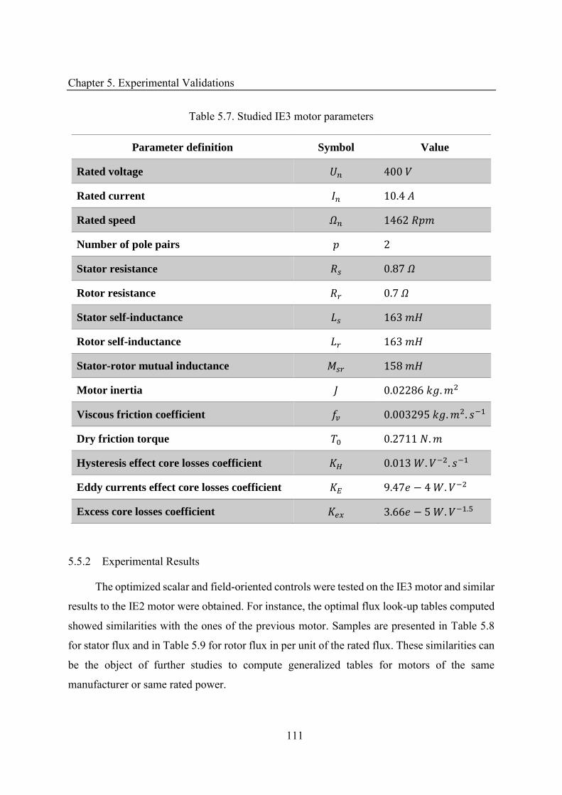
Chapter 5. Experimental Validations
111
Table 5.7. Studied IE3 motor parameters
Parameter definition Symbol Value
Rated voltage
Rated current .
Rated speed �
Number of pole pairs
Stator resistance . �
Rotor resistance . �
Stator self-inductance
Rotor self-inductance
Stator-rotor mutual inductance
Motor inertia . .
Viscous friction coefficient � . . . −
Dry friction torque . .
Hysteresis effect core losses coefficient � . . − . −
Eddy currents effect core losses coefficient . − . −
Excess core losses coefficient � . − . − .5
5.5.2 Experimental Results
The optimized scalar and field-oriented controls were tested on the IE3 motor and similar
results to the IE2 motor were obtained. For instance, the optimal flux look-up tables computed
showed similarities with the ones of the previous motor. Samples are presented in Table 5.8
for stator flux and in Table 5.9 for rotor flux in per unit of the rated flux. These similarities can
be the object of further studies to compute generalized tables for motors of the same
manufacturer or same rated power.
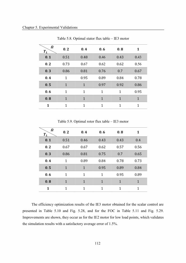
Chapter 5. Experimental Validations
112
Table 5.8. Optimal stator flux table – IE3 motor � �� . . . . . . . .46 . .43 . . .67 .62 . .56 . . . . . . . . . . . . . . . . . .
Table 5.9. Optimal rotor flux table – IE3 motor � �� . . . . . . . . . . . . . . . . . . . . . . . . . . . . . . . . . . .
The efficiency optimization results of the IE3 motor obtained for the scalar control are
presented in Table 5.10 and Fig. 5.28, and for the FOC in Table 5.11 and Fig. 5.29.
Improvements are shown, they occur as for the IE2 motor for low load points, which validates
the simulation results with a satisfactory average error of 1.5%.
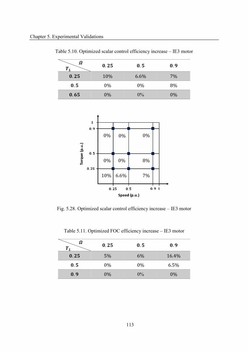
Chapter 5. Experimental Validations
113
Table 5.10. Optimized scalar control efficiency increase – IE3 motor � �� . . . . % . % % . % % % . % 0% %
Fig. 5.28. Optimized scalar control efficiency increase – IE3 motor
Table 5.11. Optimized FOC efficiency increase – IE3 motor � �� . . . . % % . % . % % . % . % 0% %
% % %
% %
% . %
%
%
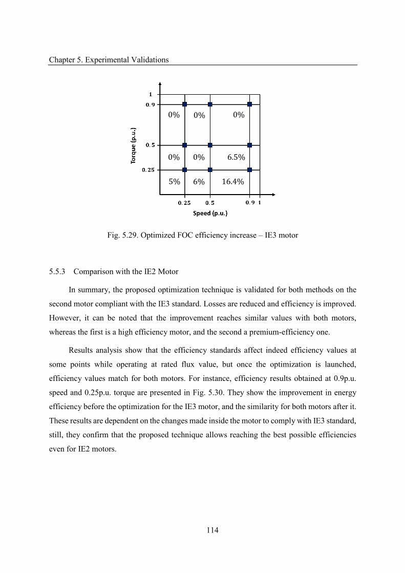
Chapter 5. Experimental Validations
114
Fig. 5.29. Optimized FOC efficiency increase – IE3 motor
5.5.3 Comparison with the IE2 Motor
In summary, the proposed optimization technique is validated for both methods on the
second motor compliant with the IE3 standard. Losses are reduced and efficiency is improved.
However, it can be noted that the improvement reaches similar values with both motors,
whereas the first is a high efficiency motor, and the second a premium-efficiency one.
Results analysis show that the efficiency standards affect indeed efficiency values at
some points while operating at rated flux value, but once the optimization is launched,
efficiency values match for both motors. For instance, efficiency results obtained at 0.9p.u.
speed and 0.25p.u. torque are presented in Fig. 5.30. They show the improvement in energy
efficiency before the optimization for the IE3 motor, and the similarity for both motors after it.
These results are dependent on the changes made inside the motor to comply with IE3 standard,
still, they confirm that the proposed technique allows reaching the best possible efficiencies
even for IE2 motors.
% % %
% . %
% %
%
. %
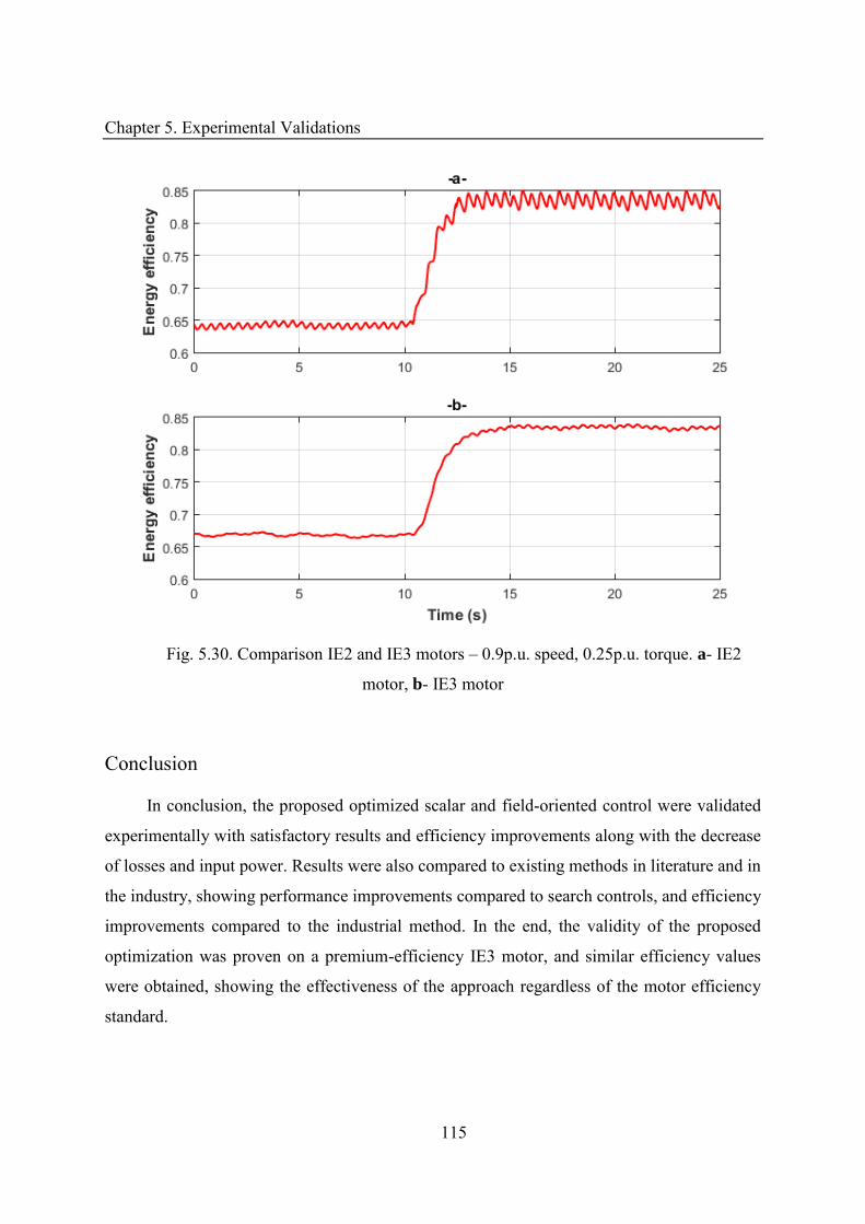
Chapter 5. Experimental Validations
115
Fig. 5.30. Comparison IE2 and IE3 motors – 0.9p.u. speed, 0.25p.u. torque. a- IE2
motor, b- IE3 motor
Conclusion
In conclusion, the proposed optimized scalar and field-oriented control were validated
experimentally with satisfactory results and efficiency improvements along with the decrease
of losses and input power. Results were also compared to existing methods in literature and in
the industry, showing performance improvements compared to search controls, and efficiency
improvements compared to the industrial method. In the end, the validity of the proposed
optimization was proven on a premium-efficiency IE3 motor, and similar efficiency values
were obtained, showing the effectiveness of the approach regardless of the motor efficiency
standard.
General Conclusion
The work presented in the present thesis concerns an energy efficiency optimization
approach of a squirrel-cage induction motor, established and applied on the scalar and field-
oriented control structures. The technique is based on optimal flux values computed using an
improved dynamic model that includes the effect of core losses. Simulation and experimental
results showed improvements compared to the classic control, and compared to the existing
optimization techniques in literature and in industry. The main points addressed and results
obtained through the study are summarized hereafter.
First, existing optimization techniques are listed in Chapter 1; they are either online
search methods, or techniques based on optimal points calculations using the classic model of
the IM. In both cases, the results lack accuracy or satisfactory performances. Thus, the
proposed approach in the thesis is based on off-line measurements to accurately map the
torque-speed plane used to optimize the reference flux. The approach is systematic and can be
established very quickly on any asynchronous machine. Moreover, the problems that occur in
the state-of-art methods are resolved in the proposed method, avoiding the delays of tracking
the optimal point and giving more accurate loss estimation.
The improved IM dynamic model presented in Chapter 2 includes the effect of the core
losses through an equivalent resistor which changes the electric and flux equations of the IM.
This resistor is continuously computed using the Bertotti core loss model which considers the
effect of the magnetic field and the voltage frequency on the losses. Through this approach, the
model dynamic computes accurately the losses and their effect on the performances. Tests
show the high precision obtained with the improved model especially in terms of core losses.
The obtained model is used to compute the equations involving the efficiency and the
flux in Chapter 3. Then, for each operating point of the torque-speed plane, the optimum flux
value is computed by systematically scanning the possible flux values and storing the value
that corresponds to the best computed efficiency in a look-up table. Results show that the
optimization is most effective at low load torques and is affected by the speed.
Consequently, the stator optimal flux table is included in the scalar control structure. It
gives the necessary flux reference, according to the measured speed and computed torque,
using a load torque observer. Similarly, the rotor optimal flux table is included in the field-
oriented control structure, as the reference of the flux loop. Simulations results presented in
General Conclusion
117
Chapter 4 show the decrease of the copper, core and inverter losses, the input power is thus
reduced and the efficiency increased. Obtained results are consistent with the theoretical ones.
Experimental tests were carried for both improved control structures as presented in
Chapter 5 on a 5.5kW IE2 standard motor, they validate the proper performances of the
structures and the efficiency increase. Tests also compare the results with the existing methods
showing improvements in terms of accuracy and dynamic performances. Moreover, another
series of tests was performed on another 5.5kW motor compliant with IE3 standard to show
the compatibility of the proposed approach. Results were positive and showed similar improved
efficiency values compared to the IE2 motor.
Furthermore, concerning the industrial implementation of the proposed technique, it
should be integrated inside the variable speed drive. The main obstacle of this approach lies in
the off-line computations of the optimal flux table required prior to the operation. However,
this process can be integrated in the drives at start-up along with the parameters estimation. It
only requires few additional minutes to estimate the core loss model coefficients and then
compute the flux table. Moreover, as detailed in the tests, several actual industrial drives use a
universal optimization technique which doesn’t give the best results for all operating points,
which confirms the need of improving these performances by implementing such a proposed
approach.
Finally, the improvement strategy proposed in this work proved to be energy efficient
and suitable for industrial use, overcoming the drawbacks of other methods. Yet, further studies
can be carried to improve the proposed control strategy as, for instance:
• Enhancing the implementation of the technique in the industrial drives by finding the
optimal size of the look-up table and analyzing similarities for motors of the same rated
power or same construction series to reduce the calculations at drive start-up,
• Developing a start-up strategy for fast drive installation including the proposed method,
• Taking into consideration the effect of temperature while optimizing the flux, or
creating a third dimension in the look-up table for this cause, and analyzing the table
robustness according to parameter variation and motor aging
• Include the inverter losses more the study and in the choice of the optimal flux,

General Conclusion
118
• Improving the scalar control structure by including a flux observer and a flux loop to
improve its stability and accuracy, as well as analyzing the need of a speed observer to
obtain a sensorless structure
• Improving the FOC by including a speed observer and an estimator of the rotor time
constant which is affected by the load torque, to increase the precision of the position
angle estimation,
• Enhancing the optimization strategy by improving its operation in transient phases, and
reaching convenient dynamic performances at start-up,
• Expanding the study to reach other types of motors, such as permanent magnet motor,
permanent magnet assisted synchronous reluctance motors, and synchronous reluctance
motors, and establishing a similar optimization technique based on their dynamic
models and control structures.

Résumé Long en Français
119
Résumé Long en Français
Introduction
L'optimisation de l'efficacité énergétique fait récemment l’objet de nombreuses
recherches, surtout dans le cas des systèmes électriques qui constituent une source essentielle
de consommation énergétique. Ainsi, la commission européenne s'est fixée l’objectif à travers
le projet Énergie-Climat d’améliorer l'efficacité énergétique des structures électriques pour
2020 dans une première étape, et puis pour 2030.
L'efficacité varie en fonction du point de fonctionnement du moteur. Ainsi pour chaque
point du plan couple-vitesse imposé par la charge, le rendement peut être optimisé en agissant
sur le flux à travers le système de commande. Plusieurs structures de contrôle peuvent être
utilisées à cette fin. Dans cette thèse, le contrôle scalaire qui est largement utilisé pour sa
simplicité, et le contrôle vectoriel indirect par orientation de flux rotorique qui est utilisé pour
sa précision et robustesse, seront étudiés.
La détermination du flux optimal nécessite la connaissance des pertes dans le système
étudié. Cependant, la plupart des études dans le domaine se basent sur le modèle dynamique
classique de la machine asynchrone qui prend en compte seulement les pertes Joule et
mécaniques. Pourtant, les pertes fer ont un effet important sur les performances de la machine,
d’où la nécessité de leur estimation et prise en compte dans l’étude. Ainsi, dans ce travail, un
modèle dynamique amélioré est proposé, prenant en compte ces pertes.
D’autre part, quelques techniques d’optimisation de l’efficacité énergétique existent dans
la littérature, mais elles manquent de précision dans certains cas et aboutissent à de mauvaises
performances dynamiques dans d’autres. Elles sont donc utilisées dans ce travail comme
méthodes comparatives pour montrer l’originalité de la technique proposée et pour en chiffrer
son efficacité.
Le présent travail propose une nouvelle approche de calcul du flux optimal permettant
l’amélioration de l’efficacité énergétique. Elle se base sur le modèle dynamique proposé de la
machine asynchrone à cage d’écureuil. La référence de flux est alors modifiée selon le point
Résumé Long en Français
120
de fonctionnement du moteur en termes de couple et de vitesse, et appliquée à la structure de
commande afin d’imposer à la machine un fonctionnement à rendement optimal.
Dans le premier chapitre, le contexte de l’étude et les standards d’efficacité énergétique
sont présentés, ainsi que les modèles de la machine et des pertes ainsi qu’un état-de-l ‘art des
techniques d’optimisation. Dans le second chapitre, le modèle dynamique amélioré est proposé.
Il sera utilisé dans le chapitre 3 pour la détermination des valeurs de flux optimal, générant
ainsi le rendement maximal. Les résultats sont stockés dans des tableaux afin d’être utilisés
dans la suite. Dans le chapitre 4, les contrôles scalaire et vectoriel optimisés sont détaillés et
simulés afin d’évaluer les résultats obtenus. Ces résultats sont ensuite validés
expérimentalement dans le chapitre 5 et comparés avec certaines méthodes existantes ainsi
qu’avec les résultats d’une machine de meilleur standard énergétique afin de comparer et
évaluer la pertinence de la proposition.
Chapitre 1 Contexte de la thèse
Dans le présent chapitre, le projet Énergie-Climat et les standards d’efficacité sont
présentés, puis les modèles de la machine asynchrone et des pertes nécessaires pour l’étude
sont détaillés. Ensuite, un tour d’horizon de l’avancement des techniques d’optimisation
d’efficacité énergétique existantes aujourd’hui est proposé.
1.1 Contexte Général
Suite à la crise économique de 2008, l’Union Européenne prit des mesures afin de
fortifier l’économie, à travers la stratégie ‘Europe 2020’ qui fixe des objectifs pour l’an 2020
selon trois axes [1]-[2] : croissance intelligente, durable et inclusive. Ainsi, dans le but de
promouvoir la recherche et l'éducation, d’améliorer l'économie, de réduire la pauvreté et le
chômage et de faire face aux défis du changement climatique, le projet Energie-Climat est mis
en œuvre avec les trois principaux objectifs :
• Réduire les émissions de gaz à effet de serre d'au moins 20% par rapport aux niveaux
de 1990, ou de 30% selon la capacité du pays,
Résumé Long en Français
121
• Augmenter de 20% l'utilisation de sources d'énergie renouvelables,
• Augmenter de 20% l'efficacité énergétique des structures électriques.
Ce projet est continuellement mis-à-jour et de nouveaux objectifs sont déjà imposés pour
l’an 2030. La question d’efficacité énergétique est alors primordiale pour les systèmes
électriques, ainsi une série de standards d’efficacité est imposée par la Commission
Internationale d’Electrotechnique (IEC) [3]-[5] pour classer les moteurs comme suit :
• IE1 : Efficacité standard
• IE2 : Haute efficacité
• IE3 : Très haute efficacité
• IE4 : Super Premium efficacité
L’objectif principal était d’atteindre des moteurs conformes au standard IE2 en 2011, et
actuellement, les objectifs visent la construction de moteurs conformes au standard IE3, ou
bien IE2 avec variateur de vitesse. Le standard IE4 n’est pas encore intégré dans les objectifs
du projet ni commercialisé, mais le sera dans les prochaines étapes. Ce travail s’intéresse à
l’optimisation du fonctionnement du moteur asynchrone à cage d’écureuil.
1.2 Etat de l’Art des Modèles de la Machine Asynchrone
La machine asynchrone est représentée par deux principaux types de modèles, dont
certaines variantes se trouvent dans la littérature : le schéma monophasé étoile équivalent
utilisé en régime permanent, et le modèle dynamique utilisé pour toutes les phases de
fonctionnement, en particulier en régime transitoire.
Concernant le schéma monophasé étoile équivalent [6]-[9], deux représentations sont
possibles, et varient au niveau des fuites magnétiques qui peuvent être représentées soit par
deux inductances de fuites partielles, l’une statorique et l’autre rotorique, soit par une
inductance de fuites globales ramenée au stator [10]. Les deux modèles donnent quasiment les
mêmes résultats, avec une représentation plus complexe mais physiquement plus juste dans le
cas des fuites partielles, face à une représentation plus simple pour les fuites globales. Pour
cela, et afin de simplifier les calculs, le schéma monophasé étoile équivalent à fuites globales,
représenté dans la Fig. 1.1, est utilisé dans cette étude.
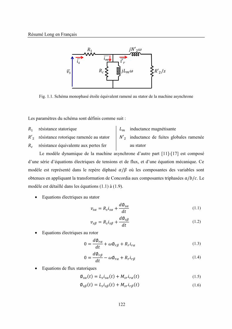
Résumé Long en Français
122
Fig. 1.1. Schéma monophasé étoile équivalent ramené au stator de la machine asynchrone
Les paramètres du schéma sont définis comme suit :
résistance statorique ′ résistance rotorique ramenée au stator
résistance équivalente aux pertes fer
inductance magnétisante ′ inductance de fuites globales ramenée
au stator
Le modèle dynamique de la machine asynchrone d’autre part [11]-[17] est composé
d’une série d’équations électriques de tensions et de flux, et d’une équation mécanique. Ce
modèle est représenté dans le repère diphasé / où les composantes des variables sont
obtenues en appliquant la transformation de Concordia aux composantes triphasées / / . Le
modèle est détaillé dans les équations (1.1) à (1.9).
• Equations électriques au stator = + ∅ (1.1)
= + ∅ (1.2)
• Equations électriques au rotor = ∅ + �∅ + (1.3)
= ∅ − �∅ + (1.4)
• Equations de flux statoriques ∅ = + (1.5) ∅ = + (1.6)
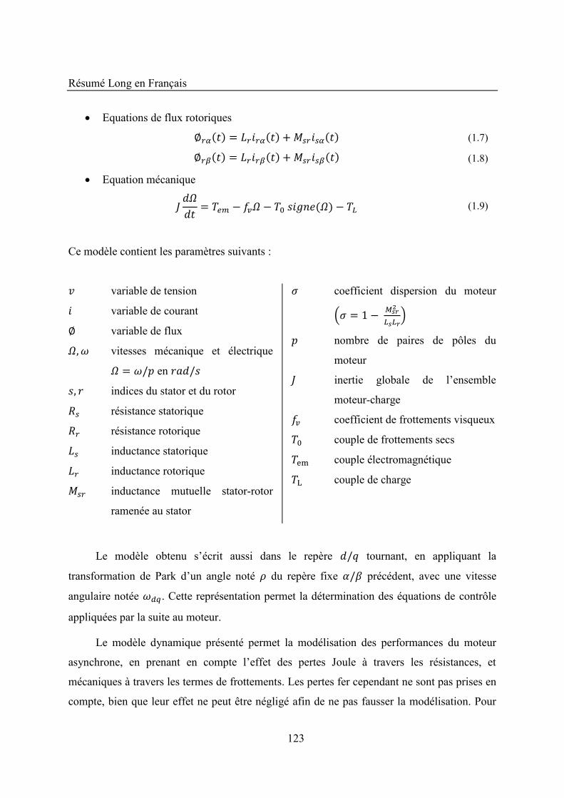
Résumé Long en Français
123
• Equations de flux rotoriques ∅ = + (1.7) ∅ = + (1.8)
• Equation mécanique � = − �� − � − (1.9)
Ce modèle contient les paramètres suivants :
variable de tension
variable de courant ∅ variable de flux �,� vitesses mécanique et électrique � = �/ en / , indices du stator et du rotor
résistance statorique
résistance rotorique
inductance statorique
inductance rotorique
inductance mutuelle stator-rotor
ramenée au stator
� coefficient dispersion du moteur � = − 2
nombre de paires de pôles du
moteur
inertie globale de l’ensemble
moteur-charge � coefficient de frottements visqueux
couple de frottements secs em couple électromagnétique L couple de charge
Le modèle obtenu s’écrit aussi dans le repère / tournant, en appliquant la
transformation de Park d’un angle noté � du repère fixe / précédent, avec une vitesse
angulaire notée � . Cette représentation permet la détermination des équations de contrôle
appliquées par la suite au moteur.
Le modèle dynamique présenté permet la modélisation des performances du moteur
asynchrone, en prenant en compte l’effet des pertes Joule à travers les résistances, et
mécaniques à travers les termes de frottements. Les pertes fer cependant ne sont pas prises en
compte, bien que leur effet ne peut être négligé afin de ne pas fausser la modélisation. Pour
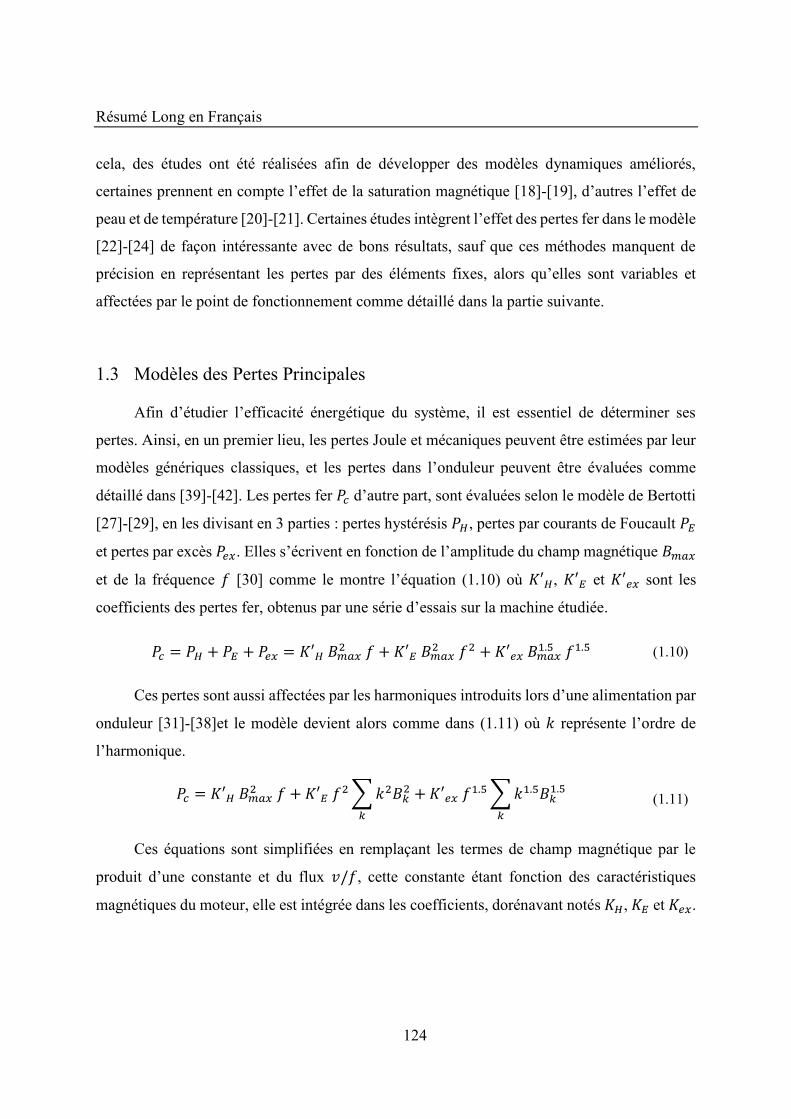
Résumé Long en Français
124
cela, des études ont été réalisées afin de développer des modèles dynamiques améliorés,
certaines prennent en compte l’effet de la saturation magnétique [18]-[19], d’autres l’effet de
peau et de température [20]-[21]. Certaines études intègrent l’effet des pertes fer dans le modèle
[22]-[24] de façon intéressante avec de bons résultats, sauf que ces méthodes manquent de
précision en représentant les pertes par des éléments fixes, alors qu’elles sont variables et
affectées par le point de fonctionnement comme détaillé dans la partie suivante.
1.3 Modèles des Pertes Principales
Afin d’étudier l’efficacité énergétique du système, il est essentiel de déterminer ses
pertes. Ainsi, en un premier lieu, les pertes Joule et mécaniques peuvent être estimées par leur
modèles génériques classiques, et les pertes dans l’onduleur peuvent être évaluées comme
détaillé dans [39]-[42]. Les pertes fer d’autre part, sont évaluées selon le modèle de Bertotti
[27]-[29], en les divisant en 3 parties : pertes hystérésis �, pertes par courants de Foucault
et pertes par excès �. Elles s’écrivent en fonction de l’amplitude du champ magnétique �
et de la fréquence [30] comme le montre l’équation (1.10) où ′�, ′ et ′ � sont les
coefficients des pertes fer, obtenus par une série d’essais sur la machine étudiée. = � + + � = ′� � + ′ � + ′ � �.5 .5 (1.10)
Ces pertes sont aussi affectées par les harmoniques introduits lors d’une alimentation par
onduleur [31]-[38]et le modèle devient alors comme dans (1.11) où représente l’ordre de
l’harmonique. = ′� � + ′ ∑ �� + ′ � .5∑ .5 �.5� (1.11)
Ces équations sont simplifiées en remplaçant les termes de champ magnétique par le
produit d’une constante et du flux / , cette constante étant fonction des caractéristiques
magnétiques du moteur, elle est intégrée dans les coefficients, dorénavant notés �, et �.
Résumé Long en Français
125
1.4 Amélioration de l’Efficacité Energétique de la Machine Asynchrone
Certains algorithmes de contrôle sont développés dans la littérature, visant l’amélioration
de l’efficacité énergétique [43]-[44], ces algorithmes s’appliquent à la structure de contrôle
classique en variant la référence de flux de façon à imposer la valeur de flux optimal selon la
stratégie d’optimisation définie.
En une première approche, le contrôle par recherche (SC) [45]-[53], modifie la consigne
de flux continuellement en ligne en surveillant la puissance absorbée, jusqu’à atteindre le
niveau de puissance minimale consommée. Une autre méthode, le contrôle par minimisation
de pertes (LMC) est développé en [54]-[64]; cette approche se base sur les modèles des pertes
afin de trouver le point optimal à travers la dérivée du modèle global. De plus, une troisième
méthode d’optimisation élaborée en littérature est la technique du couple maximal par Ampère
(MTPA) [65]-[73], basée sur une courbe de couple maximal en fonction de la pulsation qui
permet de déterminer le flux optimal à imposer, les valeurs de flux sont calculées hors-ligne de
façon à vérifier le principe du MTPA.
Les méthodes d’optimisation existantes aboutissent en effet à l’amélioration de
l’efficacité énergétique, sauf qu’elles sont accompagnées soit par des performances
dynamiques insatisfaisantes dues à l’instabilité introduite par la variation de flux continuelle,
soit par une imprécision introduite par l’approximation des pertes en vue de faciliter les calculs.
Chapitre 2 Modèle dynamique prenant en compte les pertes
fer
Le modèle dynamique classique de la machine asynchrone, formé d’équations
électriques de tensions et de flux et d’une équation mécanique, prend en compte l’effet des
pertes Joule et mécaniques et néglige l’effet des pertes fer. Ces pertes doivent être intégrées
afin d’améliorer la précision de l’étude et d’évaluer leur effet sur les performances et le bilan
énergétique du système. Dans ce chapitre, les essais de mesure et d’estimation des paramètres
des modèles sont cités, puis les méthodes d’intégration des pertes fer dans le modèle dynamique
du moteur sont détaillées.
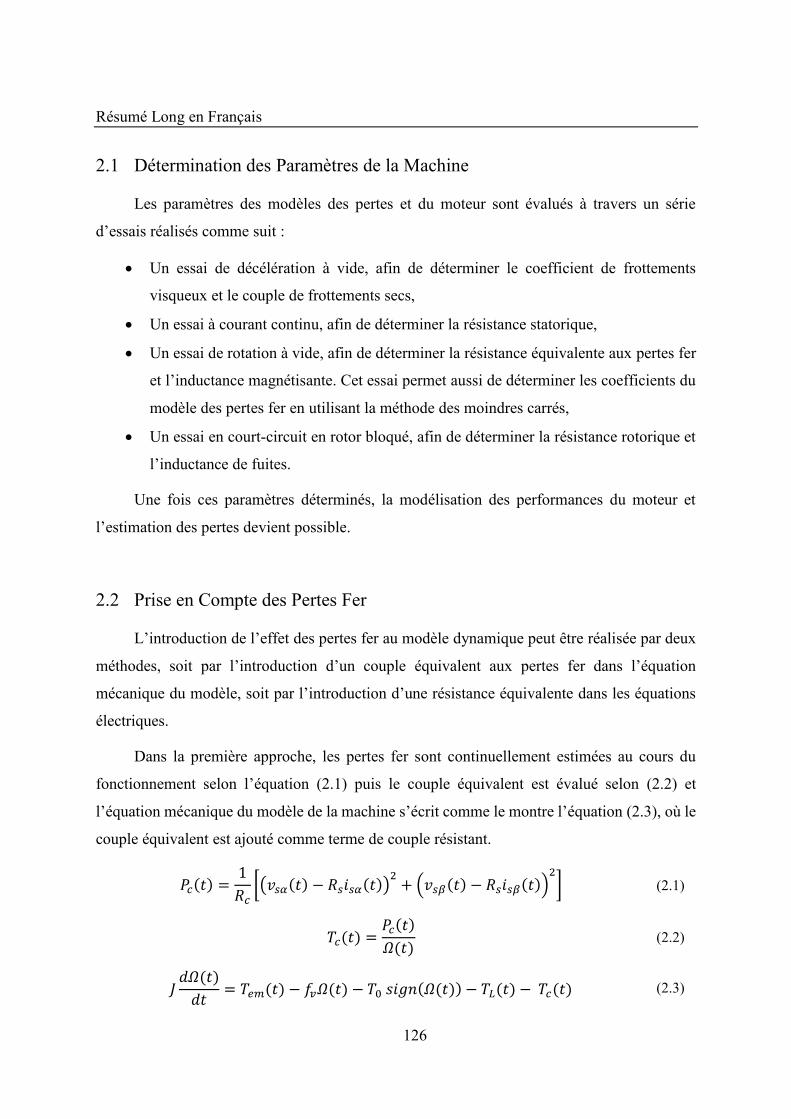
Résumé Long en Français
126
2.1 Détermination des Paramètres de la Machine
Les paramètres des modèles des pertes et du moteur sont évalués à travers un série
d’essais réalisés comme suit :
• Un essai de décélération à vide, afin de déterminer le coefficient de frottements
visqueux et le couple de frottements secs,
• Un essai à courant continu, afin de déterminer la résistance statorique,
• Un essai de rotation à vide, afin de déterminer la résistance équivalente aux pertes fer
et l’inductance magnétisante. Cet essai permet aussi de déterminer les coefficients du
modèle des pertes fer en utilisant la méthode des moindres carrés,
• Un essai en court-circuit en rotor bloqué, afin de déterminer la résistance rotorique et
l’inductance de fuites.
Une fois ces paramètres déterminés, la modélisation des performances du moteur et
l’estimation des pertes devient possible.
2.2 Prise en Compte des Pertes Fer
L’introduction de l’effet des pertes fer au modèle dynamique peut être réalisée par deux
méthodes, soit par l’introduction d’un couple équivalent aux pertes fer dans l’équation
mécanique du modèle, soit par l’introduction d’une résistance équivalente dans les équations
électriques.
Dans la première approche, les pertes fer sont continuellement estimées au cours du
fonctionnement selon l’équation (2.1) puis le couple équivalent est évalué selon (2.2) et
l’équation mécanique du modèle de la machine s’écrit comme le montre l’équation (2.3), où le
couple équivalent est ajouté comme terme de couple résistant.
= [( − ) + − ] (2.1)
= � (2.2) � = − �� − � − − (2.3)
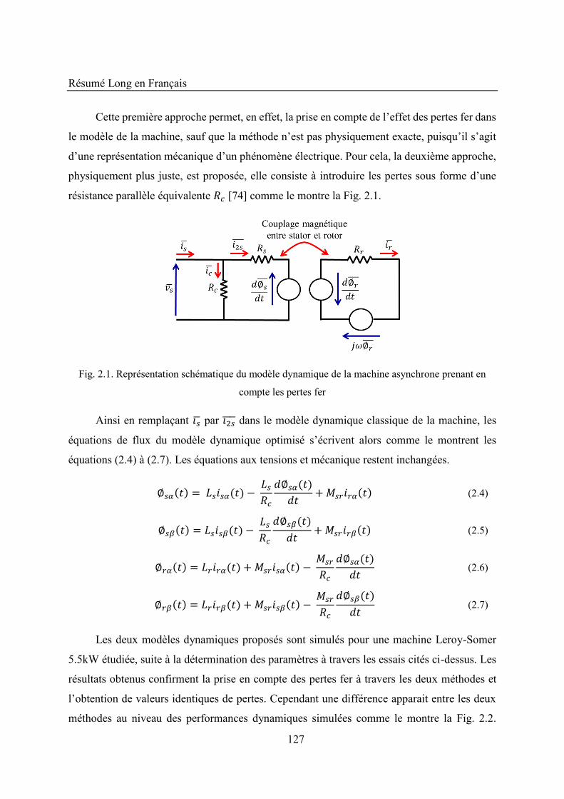
Résumé Long en Français
127
Cette première approche permet, en effet, la prise en compte de l’effet des pertes fer dans
le modèle de la machine, sauf que la méthode n’est pas physiquement exacte, puisqu’il s’agit
d’une représentation mécanique d’un phénomène électrique. Pour cela, la deuxième approche,
physiquement plus juste, est proposée, elle consiste à introduire les pertes sous forme d’une
résistance parallèle équivalente [74] comme le montre la Fig. 2.1.
Fig. 2.1. Représentation schématique du modèle dynamique de la machine asynchrone prenant en
compte les pertes fer
Ainsi en remplaçant � par � dans le modèle dynamique classique de la machine, les
équations de flux du modèle dynamique optimisé s’écrivent alors comme le montrent les
équations (2.4) à (2.7). Les équations aux tensions et mécanique restent inchangées.
∅ = − ∅ + (2.4)
∅ = − ∅ + (2.5)
∅ = + − ∅ (2.6)
∅ = + − ∅ (2.7)
Les deux modèles dynamiques proposés sont simulés pour une machine Leroy-Somer
5.5kW étudiée, suite à la détermination des paramètres à travers les essais cités ci-dessus. Les
résultats obtenus confirment la prise en compte des pertes fer à travers les deux méthodes et
l’obtention de valeurs identiques de pertes. Cependant une différence apparait entre les deux
méthodes au niveau des performances dynamiques simulées comme le montre la Fig. 2.2.
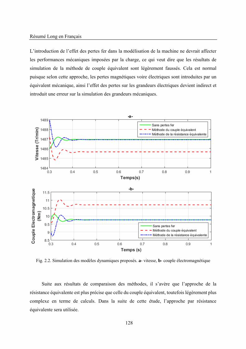
Résumé Long en Français
128
L’introduction de l’effet des pertes fer dans la modélisation de la machine ne devrait affecter
les performances mécaniques imposées par la charge, ce qui veut dire que les résultats de
simulation de la méthode de couple équivalent sont légèrement faussés. Cela est normal
puisque selon cette approche, les pertes magnétiques voire électriques sont introduites par un
équivalent mécanique, ainsi l’effet des pertes sur les grandeurs électriques devient indirect et
introduit une erreur sur la simulation des grandeurs mécaniques.
Fig. 2.2. Simulation des modèles dynamiques proposés. a- vitesse, b- couple électromagnétique
Suite aux résultats de comparaison des méthodes, il s’avère que l’approche de la
résistance équivalente est plus précise que celle du couple équivalent, toutefois légèrement plus
complexe en terme de calculs. Dans la suite de cette étude, l’approche par résistance
équivalente sera utilisée.
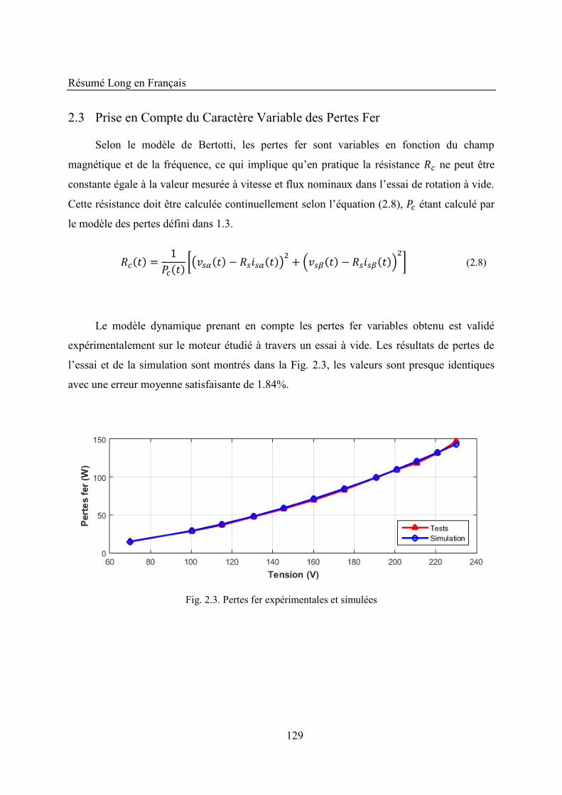
Résumé Long en Français
129
2.3 Prise en Compte du Caractère Variable des Pertes Fer
Selon le modèle de Bertotti, les pertes fer sont variables en fonction du champ
magnétique et de la fréquence, ce qui implique qu’en pratique la résistance ne peut être
constante égale à la valeur mesurée à vitesse et flux nominaux dans l’essai de rotation à vide.
Cette résistance doit être calculée continuellement selon l’équation (2.8), étant calculé par
le modèle des pertes défini dans 1.3.
= [( − ) + − ] (2.8)
Le modèle dynamique prenant en compte les pertes fer variables obtenu est validé
expérimentalement sur le moteur étudié à travers un essai à vide. Les résultats de pertes de
l’essai et de la simulation sont montrés dans la Fig. 2.3, les valeurs sont presque identiques
avec une erreur moyenne satisfaisante de 1.84%.
Fig. 2.3. Pertes fer expérimentales et simulées
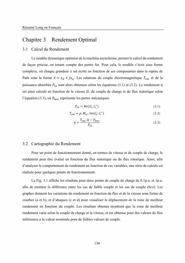
Résumé Long en Français
130
Chapitre 3 Rendement Optimal 3.1 Calcul du Rendement
Le modèle dynamique optimisé de la machine asynchrone, permet le calcul du rendement
de façon précise, en tenant compte des pertes fer. Pour cela, le modèle s’écrit sous forme
complexe, où chaque grandeur est écrite en fonction de ses composantes dans le repère de
Park sous la forme = + . Les relations du couple électromagnétique et de la
puissance absorbée � sont alors obtenues selon les équations (3.1) et (3.2). Le rendement �
est ainsi calculé en fonction de la vitesse �, du couple de charge et du flux statorique selon
l’équation (3.3), où représente les pertes mécaniques.
� = . � ∗ (3.1) = . . � . � ∗ (3.2) � = .Ω −� (3.3)
3.2 Cartographie du Rendement
Pour un point de fonctionnement donné, en termes de vitesse et de couple de charge, le
rendement peut être évalué en fonction du flux statorique ou du flux rotorique. Ainsi, afin
d’analyser le comportement du rendement en fonction de ces variables, une série de calculs est
réalisée pour quelques points de fonctionnement.
La Fig. 3.1 affiche les résultats pour deux points de couple de charge de 0.1p.u. et 1p.u.
afin de montrer la différence entre les cas de faible couple et les cas de couple élevé. Les
graphes donnent les variations du rendement en fonction du flux et de la vitesse sous forme de
courbes (a et b), et d’abaques (c et d) pour visualiser le déplacement de la zone de meilleur
rendement en fonction du couple. Les résultats obtenus montrent que la zone de meilleur
rendement varie selon le couple de charge et la vitesse, et est obtenue pour des valeurs de flux
inférieures à la valeur nominale pour de faibles valeurs de couple.
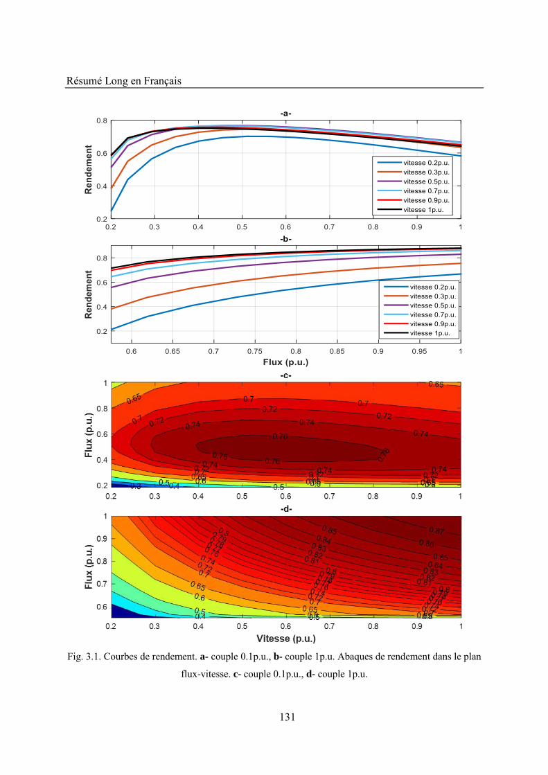
Résumé Long en Français
131
Fig. 3.1. Courbes de rendement. a- couple 0.1p.u., b- couple 1p.u. Abaques de rendement dans le plan
flux-vitesse. c- couple 0.1p.u., d- couple 1p.u.
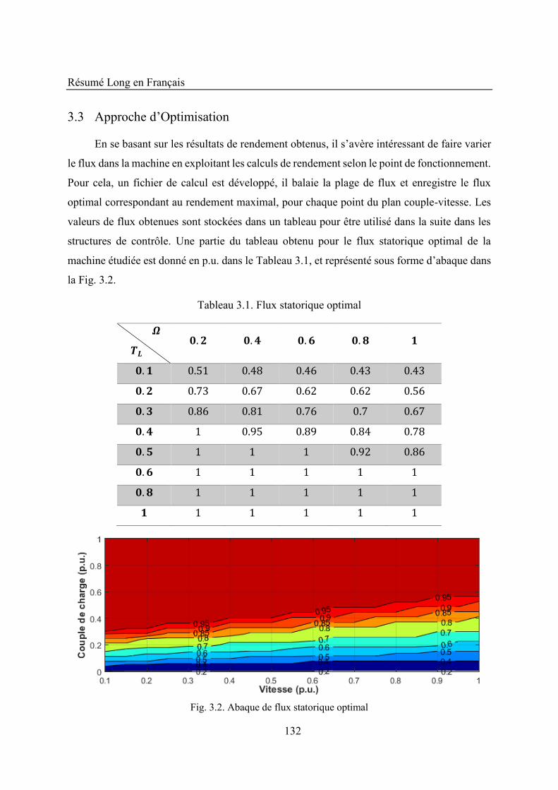
Résumé Long en Français
132
3.3 Approche d’Optimisation
En se basant sur les résultats de rendement obtenus, il s’avère intéressant de faire varier
le flux dans la machine en exploitant les calculs de rendement selon le point de fonctionnement.
Pour cela, un fichier de calcul est développé, il balaie la plage de flux et enregistre le flux
optimal correspondant au rendement maximal, pour chaque point du plan couple-vitesse. Les
valeurs de flux obtenues sont stockées dans un tableau pour être utilisé dans la suite dans les
structures de contrôle. Une partie du tableau obtenu pour le flux statorique optimal de la
machine étudiée est donné en p.u. dans le Tableau 3.1, et représenté sous forme d’abaque dans
la Fig. 3.2.
Tableau 3.1. Flux statorique optimal � �� . . . . . . . . . . . . . . . . . . . . . . . . . . . . . . . .
Fig. 3.2. Abaque de flux statorique optimal

Résumé Long en Français
133
Ces résultats montrent que le flux statorique est optimisé dans le cas de faibles charges,
par exemple pour des valeurs inférieures à 0.57p.u. à la vitesse de base (vitesse 1p.u.), et
0.31p.u. à une vitesse de 0.1p.u. Au-delà de ces valeurs, aucune optimisation n'est effectuée et
la référence de flux est égale à 1p.u. Des calculs identiques sont effectués pour tirer les valeurs
de flux rotorique optimal et des résultats très similaires sont obtenus. Il convient de noter que
le flux optimal est fonction du couple, il sera donc nécessaire d’estimer le couple de charge
pour pouvoir mettre en place cette correction.
Chapitre 4 Contrôles Optimisés
Les tableaux de flux optimal construits dans le chapitre précédent sont utilisés dans les
contrôles scalaire et vectoriel en vue d’optimiser les performances des structures de contrôle
usuelles. Ce chapitre présente les méthodes d’introduction du tableau ainsi que certains
résultats de simulation montrant l’optimisation obtenue.
4.1 Contrôle Scalaire Optimisé
Le contrôle scalaire est une structure de contrôle bien répandue dans l’industrie pour la
simplicité de son implémentation, elle est surtout utilisée dans la commande des systèmes à
pompes, compresseurs et soufflantes. Le schéma du contrôle optimisé est présenté dans la Fig.
4.1.
Le principe de ce contrôle est le réglage de l’amplitude et de la fréquence de la tension
d’alimentation selon les exigences de l’utilisateur. Pour cela, la référence de flux statorique
permet de fixer l’amplitude de la tension, qui sera imposée à la machine en utilisant la loi de
contrôle [79]-[80] présentée dans (4.1).
= ∅ √ � + � + − � � �+ � � (4.1)
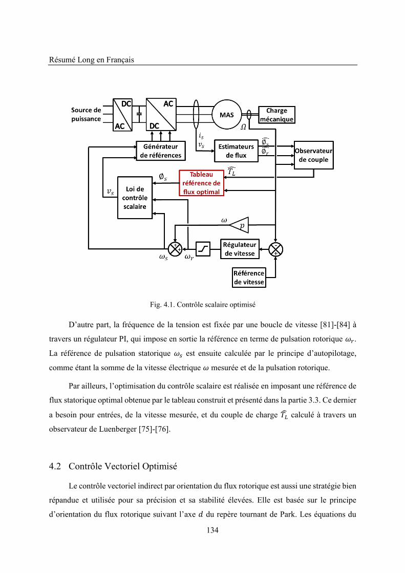
Résumé Long en Français
134
Fig. 4.1. Contrôle scalaire optimisé
D’autre part, la fréquence de la tension est fixée par une boucle de vitesse [81]-[84] à
travers un régulateur PI, qui impose en sortie la référence en terme de pulsation rotorique � .
La référence de pulsation statorique � est ensuite calculée par le principe d’autopilotage,
comme étant la somme de la vitesse électrique � mesurée et de la pulsation rotorique.
Par ailleurs, l’optimisation du contrôle scalaire est réalisée en imposant une référence de
flux statorique optimal obtenue par le tableau construit et présenté dans la partie 3.3. Ce dernier
a besoin pour entrées, de la vitesse mesurée, et du couple de charge calculé à travers un
observateur de Luenberger [75]-[76].
4.2 Contrôle Vectoriel Optimisé
Le contrôle vectoriel indirect par orientation du flux rotorique est aussi une stratégie bien
répandue et utilisée pour sa précision et sa stabilité élevées. Elle est basée sur le principe
d’orientation du flux rotorique suivant l’axe du repère tournant de Park. Les équations du
Résumé Long en Français
135
contrôle [88]-[94] découlent alors du modèle de la machine en annulant la composante du flux
rotorique suivant l’axe , comme le montrent les équations (4.2) à (4.6). représente le
courant magnétisant rotorique image du flux rotorique selon la relation ∅ = , et =/ la constante de temps rotorique.
= + � + − � − � � (4.2)
= + � + − � � + � � (4.3)
+ = (4.4)
� = � + (4.5)
= (∅ − ∅ ) = (4.6)
Le modèle de contrôle obtenu permet le dimensionnement des boucles de flux, couple et
vitesse afin de calculer les régulateurs correspondants. De plus les équations (4.4) et (4.5)
permettent l’estimation de l’angle �, en intégrant � , utilisé pour effectuer les transformations
de Park. Cependant, le contrôle obtenu se base sur le modèle de la machine sans pertes fer,
ainsi afin d’introduire l’effet de ces pertes sans avoir à changer toutes les équations du modèle,
une approximation est faite au niveau du schéma équivalent de la machine. La chute de tension
dans la résistance statorique étant faible, elle est alors déplacée à droite de la branche de .
Ainsi, le courant statorique à l’entrée du contrôle devient � = � − ���, prenant ainsi en compte
l’effet des pertes fer, et gardant la structure de base du contrôle vectoriel inchangée. La
structure globale est présentée dans la Fig. 4.2.
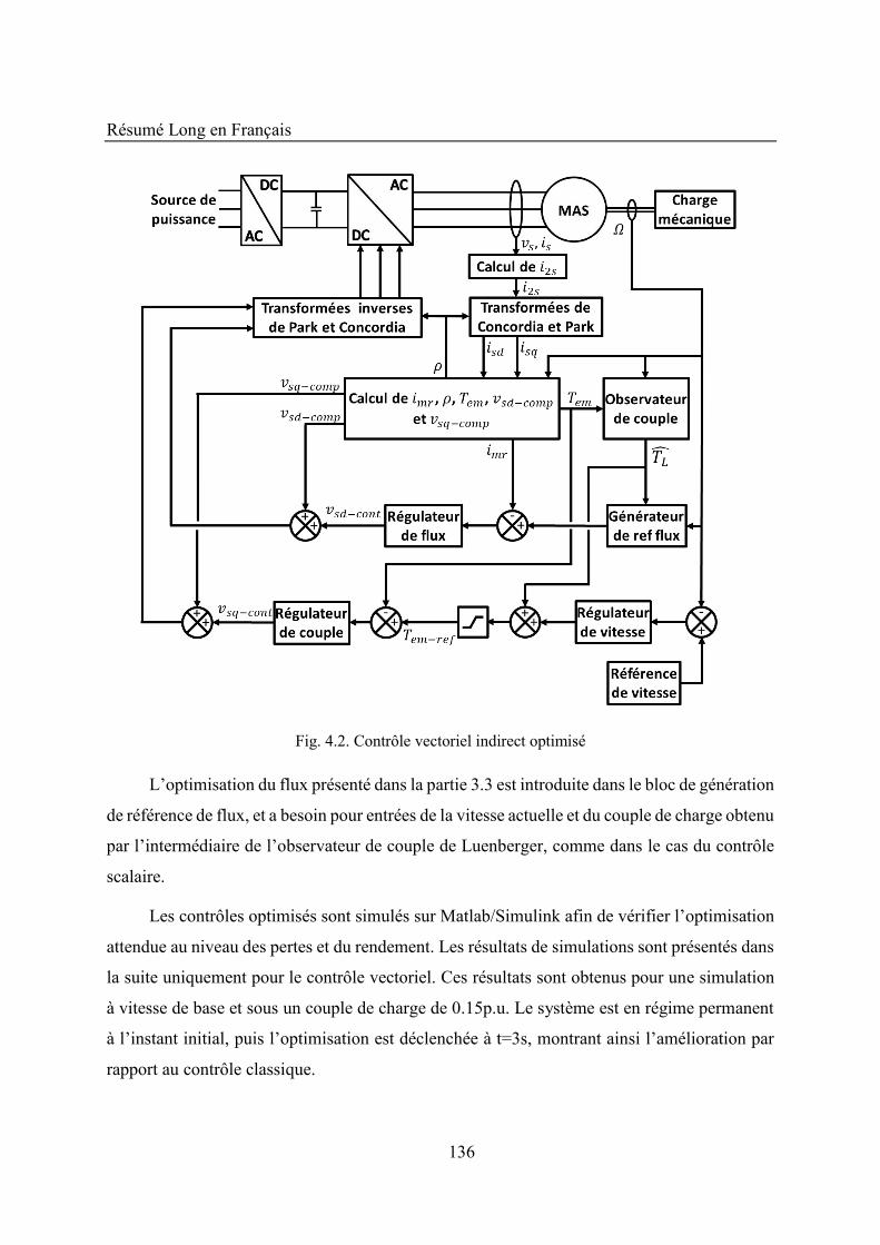
Résumé Long en Français
136
Fig. 4.2. Contrôle vectoriel indirect optimisé
L’optimisation du flux présenté dans la partie 3.3 est introduite dans le bloc de génération
de référence de flux, et a besoin pour entrées de la vitesse actuelle et du couple de charge obtenu
par l’intermédiaire de l’observateur de couple de Luenberger, comme dans le cas du contrôle
scalaire.
Les contrôles optimisés sont simulés sur Matlab/Simulink afin de vérifier l’optimisation
attendue au niveau des pertes et du rendement. Les résultats de simulations sont présentés dans
la suite uniquement pour le contrôle vectoriel. Ces résultats sont obtenus pour une simulation
à vitesse de base et sous un couple de charge de 0.15p.u. Le système est en régime permanent
à l’instant initial, puis l’optimisation est déclenchée à t=3s, montrant ainsi l’amélioration par
rapport au contrôle classique.
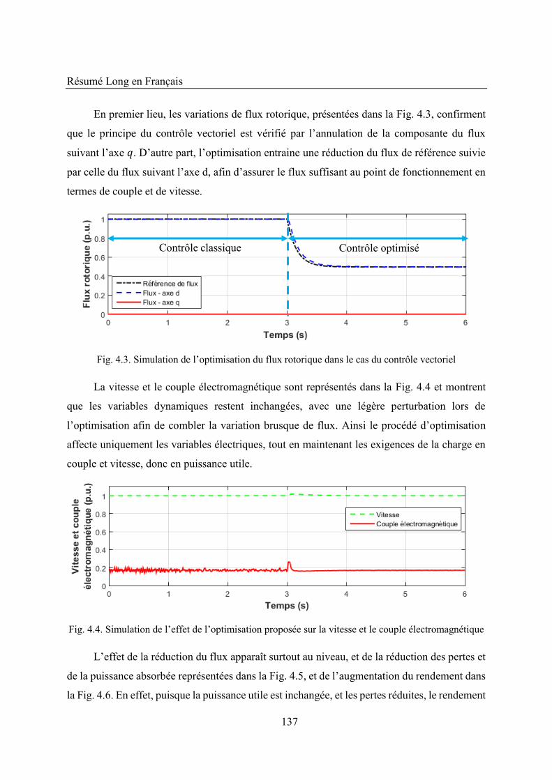
Résumé Long en Français
137
En premier lieu, les variations de flux rotorique, présentées dans la Fig. 4.3, confirment
que le principe du contrôle vectoriel est vérifié par l’annulation de la composante du flux
suivant l’axe . D’autre part, l’optimisation entraine une réduction du flux de référence suivie
par celle du flux suivant l’axe d, afin d’assurer le flux suffisant au point de fonctionnement en
termes de couple et de vitesse.
Fig. 4.3. Simulation de l’optimisation du flux rotorique dans le cas du contrôle vectoriel
La vitesse et le couple électromagnétique sont représentés dans la Fig. 4.4 et montrent
que les variables dynamiques restent inchangées, avec une légère perturbation lors de
l’optimisation afin de combler la variation brusque de flux. Ainsi le procédé d’optimisation
affecte uniquement les variables électriques, tout en maintenant les exigences de la charge en
couple et vitesse, donc en puissance utile.
Fig. 4.4. Simulation de l’effet de l’optimisation proposée sur la vitesse et le couple électromagnétique
L’effet de la réduction du flux apparaît surtout au niveau, et de la réduction des pertes et
de la puissance absorbée représentées dans la Fig. 4.5, et de l’augmentation du rendement dans
la Fig. 4.6. En effet, puisque la puissance utile est inchangée, et les pertes réduites, le rendement
Contrôle classique Contrôle optimisé
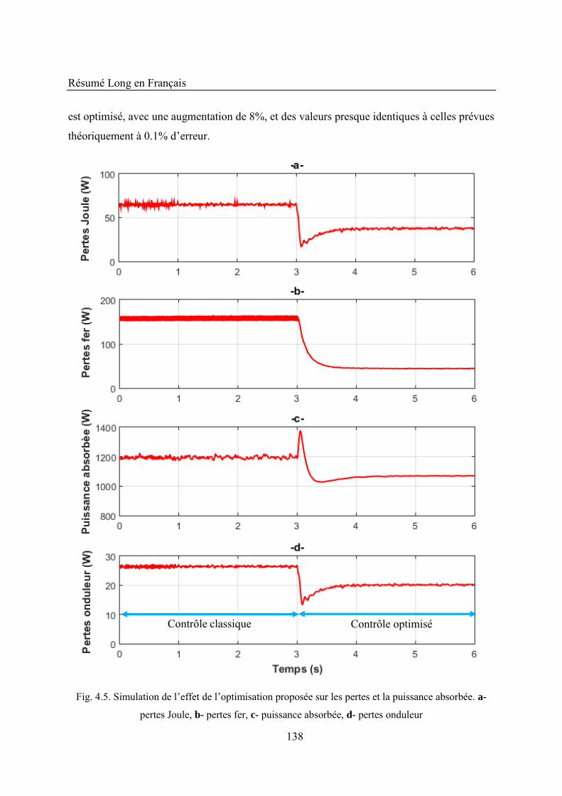
Résumé Long en Français
138
est optimisé, avec une augmentation de 8%, et des valeurs presque identiques à celles prévues
théoriquement à 0.1% d’erreur.
Fig. 4.5. Simulation de l’effet de l’optimisation proposée sur les pertes et la puissance absorbée. a-
pertes Joule, b- pertes fer, c- puissance absorbée, d- pertes onduleur
Contrôle classique Contrôle optimisé
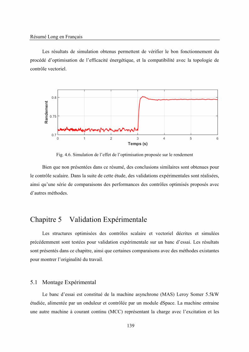
Résumé Long en Français
139
Les résultats de simulation obtenus permettent de vérifier le bon fonctionnement du
procédé d’optimisation de l’efficacité énergétique, et la compatibilité avec la topologie de
contrôle vectoriel.
Fig. 4.6. Simulation de l’effet de l’optimisation proposée sur le rendement
Bien que non présentées dans ce résumé, des conclusions similaires sont obtenues pour
le contrôle scalaire. Dans la suite de cette étude, des validations expérimentales sont réalisées,
ainsi qu’une série de comparaisons des performances des contrôles optimisés proposés avec
d’autres méthodes.
Chapitre 5 Validation Expérimentale
Les structures optimisées des contrôles scalaire et vectoriel décrites et simulées
précédemment sont testées pour validation expérimentale sur un banc d’essai. Les résultats
sont présentés dans ce chapitre, ainsi que certaines comparaisons avec des méthodes existantes
pour montrer l’originalité du travail.
5.1 Montage Expérimental
Le banc d’essai est constitué de la machine asynchrone (MAS) Leroy Somer 5.5kW
étudiée, alimentée par un onduleur et contrôlée par un module dSpace. La machine entraine
une autre machine à courant continu (MCC) représentant la charge avec l’excitation et les
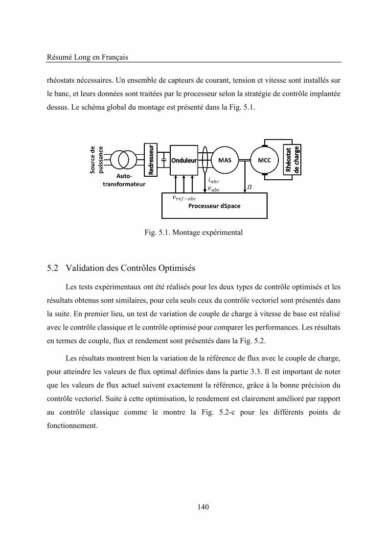
Résumé Long en Français
140
rhéostats nécessaires. Un ensemble de capteurs de courant, tension et vitesse sont installés sur
le banc, et leurs données sont traitées par le processeur selon la stratégie de contrôle implantée
dessus. Le schéma global du montage est présenté dans la Fig. 5.1.
Fig. 5.1. Montage expérimental
5.2 Validation des Contrôles Optimisés
Les tests expérimentaux ont été réalisés pour les deux types de contrôle optimisés et les
résultats obtenus sont similaires, pour cela seuls ceux du contrôle vectoriel sont présentés dans
la suite. En premier lieu, un test de variation de couple de charge à vitesse de base est réalisé
avec le contrôle classique et le contrôle optimisé pour comparer les performances. Les résultats
en termes de couple, flux et rendement sont présentés dans la Fig. 5.2.
Les résultats montrent bien la variation de la référence de flux avec le couple de charge,
pour atteindre les valeurs de flux optimal définies dans la partie 3.3. Il est important de noter
que les valeurs de flux actuel suivent exactement la référence, grâce à la bonne précision du
contrôle vectoriel. Suite à cette optimisation, le rendement est clairement amélioré par rapport
au contrôle classique comme le montre la Fig. 5.2-c pour les différents points de
fonctionnement.
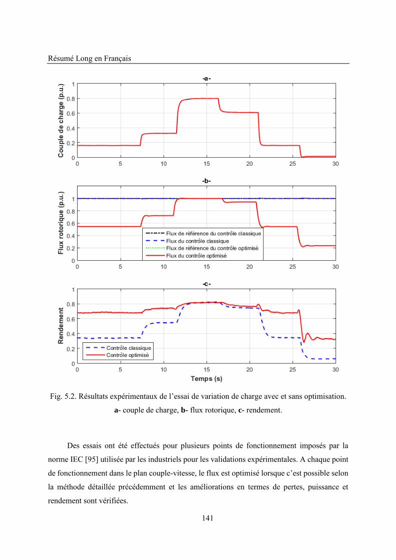
Résumé Long en Français
141
Fig. 5.2. Résultats expérimentaux de l’essai de variation de charge avec et sans optimisation.
a- couple de charge, b- flux rotorique, c- rendement.
Des essais ont été effectués pour plusieurs points de fonctionnement imposés par la
norme IEC [95] utilisée par les industriels pour les validations expérimentales. A chaque point
de fonctionnement dans le plan couple-vitesse, le flux est optimisé lorsque c’est possible selon
la méthode détaillée précédemment et les améliorations en termes de pertes, puissance et
rendement sont vérifiées.
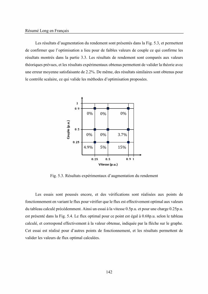
Résumé Long en Français
142
Les résultats d’augmentation du rendement sont présentés dans la Fig. 5.3, et permettent
de confirmer que l’optimisation a lieu pour de faibles valeurs de couple ce qui confirme les
résultats montrés dans la partie 3.3. Les résultats de rendement sont comparés aux valeurs
théoriques prévues, et les résultats expérimentaux obtenus permettent de valider la théorie avec
une erreur moyenne satisfaisante de 2.2%. De même, des résultats similaires sont obtenus pour
le contrôle scalaire, ce qui valide les méthodes d’optimisation proposées.
Fig. 5.3. Résultats expérimentaux d’augmentation du rendement
Les essais sont poussés encore, et des vérifications sont réalisées aux points de
fonctionnement en variant le flux pour vérifier que le flux est effectivement optimal aux valeurs
du tableau calculé précédemment. Ainsi un essai à la vitesse 0.5p.u. et pour une charge 0.25p.u.
est présenté dans la Fig. 5.4. Le flux optimal pour ce point est égal à 0.68p.u. selon le tableau
calculé, et correspond effectivement à la valeur obtenue, indiquée par la flèche sur le graphe.
Cet essai est réalisé pour d’autres points de fonctionnement, et les résultats permettent de
valider les valeurs de flux optimal calculées.
% % %
% . %
. % %
%
%
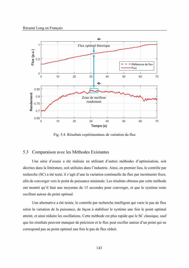
Résumé Long en Français
143
Fig. 5.4. Résultats expérimentaux de variation du flux
5.3 Comparaison avec les Méthodes Existantes
Une série d’essais a été réalisée en utilisant d’autres méthodes d’optimisation, soit
décrites dans la littérature, soit utilisées dans l’industrie. Ainsi, en premier lieu, le contrôle par
recherche (SC) a été testé, il s’agit d’une la variation continuelle du flux par incréments fixes,
afin de converger vers le point de puissance minimale. Les résultats obtenus par cette méthode
ont montré qu’il faut une moyenne de 15 secondes pour converger, et que le système reste
oscillant autour du point optimal.
Une alternative a été testée, le contrôle par recherche intelligent qui varie le pas de flux
selon la variation de la puissance, de façon à stabiliser le système une fois le point optimal
atteint, et ainsi réduire les oscillations. Cette méthode est plus rapide que le SC classique, sauf
que les résultats peuvent manquer de précision et le flux peut osciller autour d’un point qui ne
correspond pas au point optimal une fois le pas de flux réduit.
Zone de meilleur rendement
Flux optimal théorique
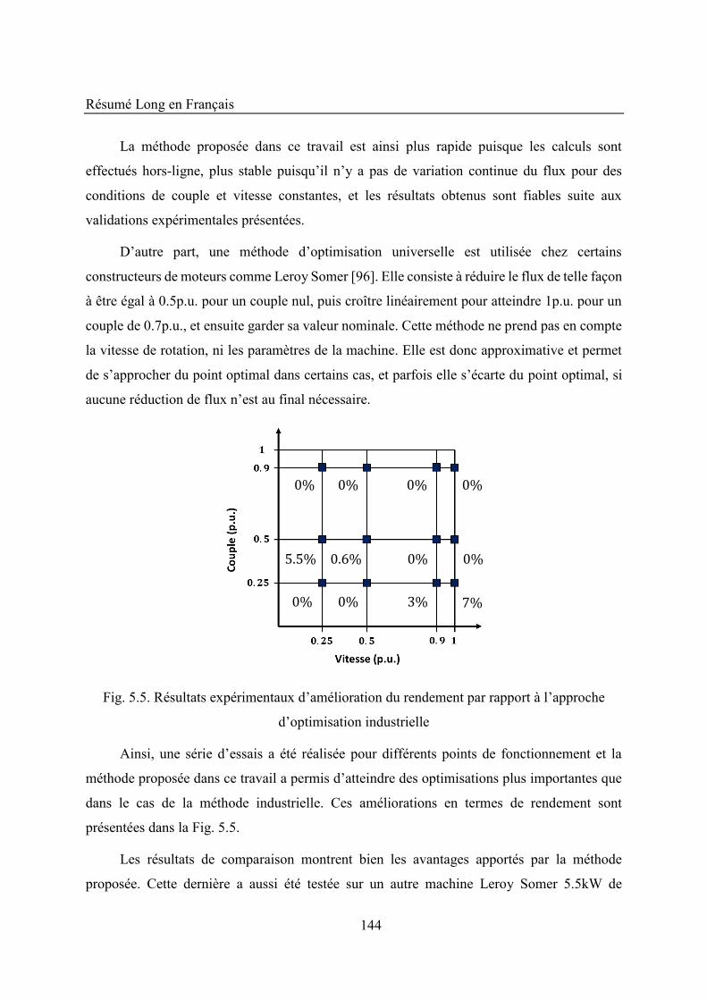
Résumé Long en Français
144
La méthode proposée dans ce travail est ainsi plus rapide puisque les calculs sont
effectués hors-ligne, plus stable puisqu’il n’y a pas de variation continue du flux pour des
conditions de couple et vitesse constantes, et les résultats obtenus sont fiables suite aux
validations expérimentales présentées.
D’autre part, une méthode d’optimisation universelle est utilisée chez certains
constructeurs de moteurs comme Leroy Somer [96]. Elle consiste à réduire le flux de telle façon
à être égal à 0.5p.u. pour un couple nul, puis croître linéairement pour atteindre 1p.u. pour un
couple de 0.7p.u., et ensuite garder sa valeur nominale. Cette méthode ne prend pas en compte
la vitesse de rotation, ni les paramètres de la machine. Elle est donc approximative et permet
de s’approcher du point optimal dans certains cas, et parfois elle s’écarte du point optimal, si
aucune réduction de flux n’est au final nécessaire.
Fig. 5.5. Résultats expérimentaux d’amélioration du rendement par rapport à l’approche
d’optimisation industrielle
Ainsi, une série d’essais a été réalisée pour différents points de fonctionnement et la
méthode proposée dans ce travail a permis d’atteindre des optimisations plus importantes que
dans le cas de la méthode industrielle. Ces améliorations en termes de rendement sont
présentées dans la Fig. 5.5.
Les résultats de comparaison montrent bien les avantages apportés par la méthode
proposée. Cette dernière a aussi été testée sur un autre machine Leroy Somer 5.5kW de
% % %
. % %
% % % %
% . %
%

Résumé Long en Français
145
génération plus récente, afin de vérifier la compatibilité de l’optimisation et évaluer les résultats
obtenus avec cette machine. Les résultats sont similaires à ceux du premier moteur dans le cas
des deux contrôles optimisés avec des valeurs de rendement similaires, malgré la différence
des standards IE2 et IE3 auxquels les machines sont conformes. Ceci montre que la méthode
d’optimisation proposée est efficace et permet de tirer le maximum de rendement même pour
les machines de faible standard énergétique.
Conclusion
Le travail présenté dans cette thèse concerne une approche d'optimisation de l'efficacité
énergétique d'un moteur asynchrone à cage d'écureuil, établie et appliquée sur les structures de
contrôles scalaire et vectoriel. La technique est basée sur la détermination de valeurs de flux
optimales calculées en utilisant un modèle dynamique amélioré qui inclut l'effet des pertes fer.
La simulation et les résultats expérimentaux ont montré des améliorations par rapport aux
contrôles classiques, et par rapport aux techniques d'optimisation existantes dans la littérature
et utilisées dans l'industrie.
Ainsi, un état-de-l’art des méthodes d’optimisation existantes et des modèles de machine et de
pertes est présenté dans le premier chapitre. Les méthodes recensées présentent des
inconvénients en termes de retard et d’imprécision. Dans le second chapitre, un modèle
dynamique de la machine asynchrone prenant en compte l’effet des pertes fer est établi.
L’estimation de ces pertes se base sur le modèle de Bertotti, et prend compte leur variation en
fonction des grandeurs du système. Dans le troisième chapitre, le calcul du rendement est
détaillé en se basant sur le modèle dynamique proposé de la machine. Les variations du
rendement en fonction du flux, du couple et de la vitesse sont alors évaluées, afin de tirer les
valeurs de flux optimal qui sont stockées dans un tableau. Ce dernier est intégré dans les
contrôles scalaire et vectoriel, ce qui fait l’objet du chapitre 4, et les résultats de simulation
présentés montrent l’efficacité de la méthode au niveau du rendement global de la machine.
Enfin le dernier chapitre présente une validation expérimentale des méthodes proposées sur
une machine conforme au standard IE2, ainsi qu’une étude comparative, basée sur des essais,
de ces méthodes avec les autres approches existantes dans la littérature et utilisées dans

Résumé Long en Français
146
l’industrie. Les essais sont aussi réalisés sur une autre machine conforme au standard
énergétique IE3 montrant ainsi la compatibilité de la démarche proposée avec d’autres
standards.
La stratégie d'amélioration proposée dans ce travail s’avère efficace et surmonte les
inconvénients majeurs des autres méthodes. Néanmoins, d'autres études peuvent être menées
pour encore améliorer la stratégie de contrôle proposée comme, par exemple :
• Trouver la meilleure façon d’installer la méthode proposée dans les variateurs de vitesse
industriels,
• Renforcer la stratégie d'optimisation en améliorant son fonctionnement en phase
transitoire, surtout au démarrage,
• Prendre en compte l'effet de la température dans l’optimisation, et analyser la robustesse
du tableau en fonction de la variation des paramètres et du vieillissement du moteur,
• Inclure les pertes onduleur dans le choix du flux optimal pour plus de précision,
• Améliorer la structure de contrôle scalaire en incluant un observateur de flux et une
boucle de flux pour améliorer sa stabilité et sa précision, ainsi qu'analyser le besoin d'un
observateur de vitesse pour obtenir une structure sans capteur,
• Améliorer le contrôle vectoriel en incluant un observateur de vitesse et un estimateur de
la constante de temps du rotor qui est affectée par le couple de charge,
• Étendre l'étude pour atteindre d'autres types de moteurs, tels que les moteurs à aimants
permanents et les moteurs synchrones à réluctance, et établir une technique
d'optimisation similaire basée sur leurs modèles dynamiques et leurs structures de
contrôle.
References
147
References
[1] Europe 2020, A strategy for smart, sustainable and inclusive growth, European Commission, Brussels, 2010.
[2] A policy framework for climate and energy in the period from 2020 to 2030, Communication from the commission to the European parliament, the council, the European economic and social committee and the committee of the regions, European Commission, Brussels, 2014.
[3] Guidelines accompanying Commission Regulations (EC) No 640/2009 of 22 July 2009 implementing Directive 2005/32/EC with regard to Ecodesign Requirements for Electric Motors and No 4/2014 of 6 January 2014 amending Regulation (EC) No 640/2009, European Commission, 2014.
[4] IEC 60034-30-1, Efficiency classes of line operated AC motors (IE code), 2014.
[5] F. Ferreira, G. Baoming, A. Almeida, Reliability and Operation of High-Efficiency Induction Motors, IEEE Trans. Industry Applications, vol. 52, no. 6, pp. 4628-4637, 2016.
[6] B. Johnson, J. Willis, Tailoring induction motor analytical models to fit known motor performance characteristics and satisfy particular study needs, IEEE Trans. Power Systems, vol. 6, no. 3, pp. 959-965, 1991.
[7] J. Guemes, J. Del Hoyo, On-load Modelling of Three-phase Induction Motors. A New Method for Determination of the Rated Current and Equivalent Circuit Parameters, Proc. IEEE Int. Conf. Industry Applications, pp. 352-358, Italy, 2002.
[8] M. Fan, J. Chai, X. Sun, Induction Motor Parameter Identification Based on T-model Equivalent Circuit, Proc. IEEE Int. Conf. Electrical Machines and Systems, pp. 2535-2539, China, 2014.
[9] D. O’Kelly, Three-phase Induction Machine, Performance and control of electrical machines, McGraw-Hill UK, pp. 241-281, 1991.
[10] A. Hughes, Induction Motor Equivalent Circuit, Electric Motors and Drives, Fundamentals, Types and Applications, Elsevier, Newnes, third edition, pp. 236-277, 2008. [11] J. Chatelain, Machines électriques, Dunod, Tome 1, pp. 225-257, 1983.
[12] A. Leedy, Simulink/MATLAB Dynamic Induction Motor Model for use in Undergraduate Electric Machines and Power Electronics Courses, IEEE Proc. Southeastcon, 2013.
[13] W. Pawlus, M. Choux, G. Hovland, V. Huynh, Parameters Identification of Induction Motor Dynamic Model for Offshore Applications, Proc. IEEE/ASME Int. Conf. Mechatronic and Embedded Systems and Applications, 2014.
[14] E. Madhuri, R. Kalpana, K. Anuradha, Performance analysis of Inverter fed Induction Motor with minimum settling time control, Proc. IEEE Int. Conf. Power Electronics, Drives and Energy Systems, 2012.
[15] I. Boldea, S.A., Vector Control of AC Drives, CRC Press, 1992.
[16] P. Vas, Monitoring Various Machine Parameters, Parameter Estimation, Condition
References
148
Monitoring and Diagnosis of Electrical Machines, Oxford Science Publications, pp. 180-189, 1993. [17] G. Slemon, Modelling of Induction Machines for Electric Drives, IEEE Trans. Industry Applications, vol. 25, no. 6, pp. 1126-1131, 1989. [18] Z. Qu, M. Ranta, M. Hinkkanen, J. Luomi, Loss-Minimizing Flux Level Control of Induction Motor Drives, IEEE Trans. Industry Applications, vol. 48, no. 3, pp. 952-961, 2012.
[19] T. Tuovinen, M. Hinkkanen, J. Luomi, Modeling of Saturation Due to Main and Leakage Flux Interaction in Induction Machines, IEEE Trans. Industry Applications, vol. 46, no. 3, pp. 937-945, 2010.
[20] E. Filho, R. De Souza, Three-phase Induction Motor Dynamic Mathematical Model, Proc. IEEE Int. Conf. Electric Machines and Drives, pp. MB1/2.1 - MB1/2.3, 1997.
[21] S. Canat, J. Faucher, Modeling and simulation of induction machine with fractional derivative, Proc. IFAC workshop on fractional differentiation and its applications, pp. 393-399, 2004.
[22] E. Levi, Iron Core Loss Effects in Indirect Rotor Flux Oriented Induction Machines, Proc. Mediterranean Electrotechnical Conference, pp. 766-769, Turkey, 1994.
[23] G. Garcia, J. Santisteban, S. Brignone, Iron Losses Influence on A Field-Oriented Controller, Proc. Int. Conf. Industrial Electronics, Control and Instrumentation, pp. 633-638, Italy, 1994.
[24] J. Choi, D. Chung, S. Sul, Implementation of Field Oriented Induction Machine Considering Iron Losses, Proc. Int. Conf. Applied Power Electronics, pp. 375-379, USA, 1996.
[25] A. Frias, Minimisation des pertes fer des machines électriques de traction par la modélisation et l'optimisation, Ph.D. thesis of Université de Grenoble, 2015.
[26] T Chevalier, Modélisation et mesure des pertes fer dans les machines électriques, application à la machine asynchrone, Ph.D. thesis of Institut National Polytechnique de Grenoble, 1999.
[27] M. Fratila, A. Benabou, A. Tounzi, M. Dessoude, Calculation of Iron Losses in Solid Rotor Induction Machine Using FEM, IEEE Trans. Magnetics, vol. 50, no. 2, 2014.
[28] G. Bertotti, F. Fiorillo, G. Soardo. The Prediction of Power Losses in Soft Magnetic Materials, Journal de Physique, vol. 49, no. C8, pp. 1915-1919, 1988.
[29] G. Bertotti, General Properties of Power Losses in Soft Ferromagnetic Materials, IEEE Trans. Magnetics, vo1. 24, no. 1, pp. 621-630, 1988.
[30] R. Romary, K. Komeza, M. Dems, J. Brudny, D. Roger, Analytical and field-circuit core loss prediction in induction motor, Przeglad Elektrotechniczny, vol. 88, no. 7b, pp. 127-130, 2012.
[31] K. Komeza, M. Dems, Finite-Element and Analytical Calculations of No-Load Core Losses in Energy-Saving Induction Motors, IEEE Trans. Industrial Electronics, vol. 59, no. 7, pp. 2934-2946, 2012.
[32] A. Boglietti, P. Ferraris, M. Lazzari, M. Pastorelli, Change of the Iron Losses with the Switching Supply Frequency in Soft Magnetic Materials Supplied by PWM Inverter, IEEE
References
149
Trans. Magnetics, vol. 31, no. 6, 1995.
[33] F. Fiorillo, A. Novikov, An Improved Approach to Power Losses in Magnetic Laminations under Nonsinusoidal Induction Waveform, IEEE Trans. Magnetics, vol. 26, no. 5, pp. 2904-2910, 1990. [34] A. Boglietti, A. Cavagnino, M. Lazzari, M. Pastorelli, Predicting Iron Losses in Soft Magnetic Materials with Arbitrary Voltage Supply: An Engineering Approach, IEEE Trans. Magnetics, vol. 39, no. 2, pp. 981–989, 2003.
[35] H. Wang, J. Wu, The Calculation of Iron Losses in Inverter-fed Induction Motors Based on Time-stepping FEM, Proc. Int. Conf. Electrical Machines and Systems, pp. 818-821, Korea, 2013.
[36] D. Kowal, P. Sergeant, L. Dupré, L. Vandenbossche, Comparison of Iron Loss Models for Electrical Machines with Different Frequency Domain and Time Domain Methods for Excess Loss Prediction, IEEE Trans. Magnetics, vol. 51, no. 1, pp. 1-10, 2015.
[37] B. Zhang, M. Doppelbauer, Numerical Iron Loss Calculation of a New Axial Flux Machine with Segmented-Armature-Torus Topology, IET Int. Conf. Power Electronics, Machines and Drives, Manchester, 2014.
[38] W. Tsai, A Study on Core Losses of Non-Oriented Electrical Steel Laminations under Sinusoidal, Non-sinusoidal and PWM Voltage Supplies, Proc. IEEE int. Region 10 conf., Taiwan, 2007.
[39] A. Fratta, F. Scapino, Modelling inverter losses for circuit simulation, Int. Conf. Power Electronics Specialists Conference, pp. 4479–4485, Germany, 2004.
[40] Z. Xuhui, W. Xuhui, G. Xinhua, Z. Feng, Analysis of Voltage Source Inverter Losses Model, Int. Conf. Electric Information and Control Engineering, pp. 5704 – 5707, China, 2011.
[41] Y. Yao, D. Lu, D. Verstraete, Power Loss Modelling of MOSFET Inverter for Low-Power Permanent Magnet Synchronous Motor Drive, Proc. Int. Conf. Future Energy Electronics, pp. 849-854, 2013.
[42] M. Saur, B. Piepenbreier, W. Xu, R. Lorenz, Implementation and Evaluation of Inverter Loss Modeling as Part of DB-DTFC for Loss Minimization Each Switching Period, Proc. IEEE Int. Conf. Power Electronics and Applications, Finland, 2014.
[43] D. Kirschen, D. Novotny, W. Suwanwisoot, Minimizing Induction Motor Losses by Excitation Control in Variable Frequency Drives, IEEE Trans. Industry Applications, vol. IA-20, no. 5, pp. 1244-1250, 1984.
[44] C. Thanga Raj, S. Srivastava, P. Agarwal, Energy Efficient Control of Three-Phase Induction Motor - A Review, International Journal of Computer and Electrical Engineering, vol. 1, no. 1, 2009.
[45] J. Cleland, V. McCormick, M. Turner, Design of an Efficiency Optimization Controller for Inverter-fed AC Induction Motors, Proc. Int. Conf. Industry Applications Conference, pp. 16-21, Florida, 1995.
[46] P. Famouri, J. Cathey, Loss Minimization Control of an Induction Motor Drive, Proc. Int. Industry Applications Society Conf., California, 1989.
References
150
[47] D. Kirschen, D. Novotny, T. Lipo, On-line Efficiency Optimization of a Variable Frequency Induction Motor Drive, IEEE Trans. Industry Applications, vol. IA-21, no. 4, pp. 610-616, 1985.
[48] C. Ta, Y. Hori, Convergence improvement of efficiency-optimization control of induction motor drives, IEEE Trans. Industry Applications, vol. 37, no. 6, pp. 1746-1753, 2001. [49] Y. Li, H. Yu, Energy-Optimized Fuzzy Control of Induction Motors Based on Nonintrusive Efficiency Estimation, Proc. IEEE Int. Conf. Control Applications, Singapore, pp. 1134-1137, 2007.
[50] Z. Rouabah, F. Zidani, B. Abdelhadi, Fuzzy efficiency enhancement of induction motor drive, Proc. Int. Conf. Power Engineering, Energy and Electrical Drives, Turkey, 2013.
[51] J. Moreno, M. Cipolla, J. Peracaula, P. Da Costa Branco, Fuzzy logic based improvements in efficiency optimization of induction motor drives, Proc. Int. Conf. Fuzzy Systems, Barcelona, 1997.
[52] B. Bose, N. Patel, K. Rajashekara, A Neuro-Fuzzy Base On-line Efficiency Optimization Control of a Stator Flux Oriented Direct Vector Controlled Induction Motor Drive, IEEE Trans. Industrial Electronics, vol. 44, no. 2, pp. 270-273, 1997.
[53] G. Sousa, B. Bose, J. Cleland, Fuzzy logic based on-line efficiency optimization control of an indirect vector-controlled induction motor drive, IEEE Trans. Industrial Electronics, vol. 42, no. 2, pp. 192-198, 1995.
[54] M. Waheedabeevi, A. Sukeshkumar, N. Nair, New online loss- minimization-based control of scalar and vector-controlled induction motor drives, Proc. IEEE Int. Conf. Power Electronics, Drives and Energy Systems, pp. 1-7, India, 2012.
[55] A. Kusko, D. Galler, Control Means for Minimization of Losses in AC and DC Motor Drives, IEEE Trans. Industry Applications, vol. 1A-19, no. 4, 1983.
[56] G. Garcia, J. Mendes Luis, R. Stephan, E. Watanabe, An Efficient Controller for an Adjustable Speed Induction Motor Drive, IEEE Trans. Industrial Electronics, vol. 41, no. 5, pp. 533-539, 1994.
[57] P. Bastiani, Stratégies de commande minimisant les pertes d'un ensemble convertisseur - machine alternative : Application à la traction électrique, Ph.D. thesis of Institut National des Sciences Appliquées de Lyon, 2001.
[58] M. Farasat, A. Trzynadlowski, M. Fadali, Efficiency improved sensorless control scheme for electric vehicle induction motors, IET Electrical Systems in Transportation, vol. 4, no. 4, pp. 122-131, 2014.
[59] D. Casadei, M. Mengoni, G. Serra, A. Tani, L. Zarri, M. Cabanas, Energy-Efficient Control of Induction Motors for Automotive Applications, Proc. Int. Conf. Electrical Machines, Italy, 2010.
[60] A. Borisevich, G. Schullerus, Energy Efficient Control of an Induction Machine Under Torque Step Changes, IEEE Trans. Energy Conversion, vol. 31, no. 4, pp. 1295-1303, 2016.
[61] S. Vukosavic, E. Levi, Robust DSP-Based Efficiency Optimization of a Variable Speed Induction Motor Drive, IEEE Trans. Industrial Electronics, vol. 50, no. 3, pp. 560-570, 2003.
References
151
[62] R. Yanamshetti, S. Bharatkar, D. Chatterjee, A. Ganguli, A Dynamic Search Technique for Efficiency Optimization for Variable Speed Induction Machine, Proc. IEEE Int. Conf. Industrial Electronics and Applications, pp. 1038-1042, China, 2009
[63] A. Scarmin, C. Gnoatto, E. Aguiar, H. Camara, E. Carati, Hybrid Adaptive Efficiency Control Technique for Energy Optimization in Induction Motor Drives, Proc. IEEE/IAS Int. Conf. Industry Applications, Brazil, 2010.
[64] I. Kioskeridis, N. Margaris, Loss minimization in induction motor adjustable speed drives, IEEE Trans. Industrial Electronics, vol. 43, no. 1, pp. 226-231, 2014.
[65] M. Cacciato, A. Consoli, G. Scarcella, G. Scelba, A. Testa, Efficiency Optimization Techniques via Constant Optimal Slip Control of Induction Motor Drives, Proc. IEEE Int. Conf. Power Electronics, Electrical Drives, Automation and Motion, Italy, pp. 33-38, 2006.
[66] M. Saur, B. Lehner, F. Hentschel, D. Gerling, R. Lorenz, DB-DTFC as Loss Minimizing Control for Synchronous Reluctance Drives, Proc. IEEE Industrial Electronics Society Int. Conf., pp. 1412-1417, Japan, 2015.
[67] R. Bojoi, Z. Li, S. Odhano, G. Griva, A. Tenconi, Unified Direct-Flux Vector Control of Induction Motor Drives with Maximum Torque per Ampere Operation, Proc. IEEE Int. Energy Conversion Congress and Exposition, pp. 3888-3895, Denver, 2013.
[68] H. Ouadi, F. Giri, A. Elfadili, L. Dugard, Induction Machine Speed Control with Flux Optimization, Control Engineering Practice, Elsevier, vol. 18, no. 1, pp. 55-66, 2010.
[69] O. Wasynczuk, S. Sudhoff, K. Corzine, J. Tichenor, P. Krause, I. Hamen, L. Taylor, A Maximum Torque per Ampere Control Strategy for Induction Motor Drives, IEEE Trans. Energy Conversion, vol. 13, no. 2, pp. 163-169, 1998.
[70] S. Peresada, S. Kovbasa, S. Dymko, S. Bozhko, Dynamic Output Feedback Linearizing Control of Saturated Induction Motors with Torque per Ampere Ratio Maximization, Proc. Int. Conf. Intelligent Energy and Power Systems, Ukraine, 2016.
[71] N. Sidek, N. Rosmin, H. Rahman, M. Hassan, F. Hussin, A. Musta'amal, Efficiency Optimization of an Induction Machine using Optimal Flux Control, Proc. IEEE Int. Conf. Energy Conversion, pp. 219-224, Malaysia, 2014.
[72] S. Bozhko, S. Dymko, S. Kovbasa, S. Peresada, Maximum Torque-per-Amp Control for Traction IM Drives: Theory and Experimental Results, IEEE Trans. Industry Applications, vol. 53, no. 1, pp. 181-193, 2017.
[73] G. Zhou, J. Ahn, A Novel Efficiency Optimization Strategy of IPMSM for Pump Applications, Journal of Electrical Engineering & Technology, vol. 4, no. 4, pp. 515-520, 2009.
[74] D. Chatterjee, Impact of core losses on parameter identification of three-phase induction machines, IET Trans. Power Electronics, vol. 7, no. 12, pp. 3126-3136, 2014.
[75] B. De Fornel, J. Louis, Electrical Actuators, Identification and Observation, Wiley, pp. 360-375, 2010.
[76] R. Ghosn, Contrôle vectoriel de la machine asynchrone à rotor bobiné à double alimentation, Ph.D. thesis, ENSEEIHT, INP, Toulouse, 2001.
[77] S. El Khil, I. Slama-Belkhodja, M. Pietrzak-David, B. de Fornel, Sensorless Field
References
152
Oriented Control of Doubly Fed Induction Speed Drive, Proc. Int. Conf. Computer as a Tool, pp. 1888-1895, Warsaw, 2007.
[78] S. Di Gennaro, J. Domínguez, M. Meza, Sensorless High Order Sliding Mode Control of Induction Motors with Core Loss, IEEE Trans. Industrial Electronics, vol. 61, no. 6, pp. 2678-2689, 2014. [79] S. Nasar, I. Boldea, Electric Machines Dynamics and Control, CRC, pp. 113-184, 1993.
[80] F. Bordry, B. De Fornel, B. Trannoy, Flux and speed numerical control of a voltage-fed asynchronous induction machine, Proc. IEE Electric Power Applications, vol. 127, no. 2, pp. 91-95, 1980.
[81] R. Sangrody, J. Nazarzadeh, K. Nikravesh, Bifurcation and Lyapunov’s exponents characteristics of electrical scalar drive systems, IET Power Electronics, vol. 5, no. 7, pp. 1236-1244, 2012.
[82] D. Karthik, T. Chelliah, Analysis of Scalar and Vector Control Based Efficiency-Optimized Induction Motors Subjected to Inverter and Sensor Faults, Proc. Int. Conf. Advanced Communication Control and Computing Technologies, pp. 462-466, India, 2016.
[83] S. Pati, S. Mohanty, M. Patnaik, Improvement of Transient and Steady State Performance of a Scalar Controlled Induction Motor Using Sliding Mode Controller, Proc. Int. Conf. Circuit, Power and Computing Technologies, pp. 220-225, India, 2015.
[84] C. Wang, C. Fang, Sensorless Scalar-Controlled Induction Motor Drives with Modified Flux Observer, IEEE Trans. Energy Conversion, vol. 18, no. 2, pp. 181-186, 2003.
[85] A. Draou, A. Miloud, Y. Miloud, A Variable Gains PI Speed Controller in a Simplified Scalar Mode Control Induction Machine Drive - Design and Implementation, Proc. Int. Conf. Control, Automation and Systems, Korea, pp. 2467-2471, 2010.
[86] S. Jin, Z. Wei, H. Zhenyi, One Novel Scalar Control Scheme for Induction Machine, Proc. Int. Conf. of IEEE Industrial Electronics Society (IECON), Korea, pp. 347-352, 2004. [87] P. Seixas, Commande numérique d'une machine synchrone autopilotée : méthode algébrique de modulation de largeur d'impulsion : algorithmes de contrôle et de régulation des courants, Ph.D. Thesis, LEEI, INP, Toulouse, 1988. [88] F. Mapelli, A. Bezzolato, D. Tarsitano, A Rotor Resistance MRAS Estimator for Induction Motor Traction Drive for Electrical Vehicles, Proc. Int. Conf. Electrical Machines, pp. 823-829, France, 2012. [89] F. Blaschke, The Principle of Field-Orientation as Applied to the Transvector Closed-Loop Control System for Rotating-Field Machines, Siemens Rev., vol. 34, pp. 217–220, 1972.
[90] J. Finch, D. Giaouris, Controlled AC Electrical Drives, IEEE Trans. Industrial Electronics, vol. 55, no. 2, pp. 481 – 491, 2008.
[91] G. Buja, M. Kazmierkowski, Direct Torque Control of PWM Inverter-Fed AC Motors - a Survey, IEEE Trans. Industrial Electronics, vol. 51, no. 4, pp. 744–757, 2004.
[92] D. Casadei, F. Profumo, G. Serra, A. Tani, FOC and DTC: Two Viable Schemes for Induction Motors Torque Control, IEEE Trans. Power Electronics, vol. 17, pp. 779–787, 2002.
[93] F. Mapelli, D. Tarsitano, M. Mauri, Plug-In Hybrid Electric Vehicle: Modeling, Prototype

References
153
Realization, and Inverter Losses Reduction Analysis, IEEE Trans. Industrial Electronics, vol. 57, no. 2, pp. 598-607, 2010. [94] G. Garcia, R. Stephan, E. Watanabe, Comparing the Indirect Field-Oriented Control with a Scalar Method, IEEE Trans. Industrial Electronics, vol. 41, no. 2, pp. 201–207, 1994. [95] IEC 60034-30-2, Rotating Electrical Machines, Efficiency classes of variable speed AC motors (IE code), 2015.
[96] Leroy Somer - Nidec, Unidrive M701 Parameter Reference Guide, Issue 01.16.01.00, p. 133, 2016.
References
154
List of Publications Published Conference Papers
1. Gabriel Khoury, Ragi Ghosn, Flavia Khatounian, Maurice Fadel, Mathias Tientcheu,
Including Core Losses in Induction Motors Dynamic Model, Proc. IEEE Int. Conf.
Renewable Energies for Developing countries, Lebanon, 2016.
2. Gabriel Khoury, Ragi Ghosn, Flavia Khatounian, Maurice Fadel, Mathias Tientcheu,
An improved Dynamic Model for Induction Motors Including Core Losses, Proc. Int.
Conf. Power Electronics and Motion Control, Bulgaria, 2016.
3. Gabriel Khoury, Ragi Ghosn, Flavia Khatounian, Maurice Fadel, Mathias Tientcheu,
Scalar Control Optimization Technique Taking into Account Core Losses for an
Induction Motor, Proc. Int. Conf. Theory and Application of Modeling and Simulation
in Electrical Power Engineering, ELECTRIMACS, 2017.
Accepted Journal Paper
4. Gabriel Khoury, Ragi Ghosn, Flavia Khatounian, Maurice Fadel, Mathias Tientcheu,
An Energy Efficient Scalar Control Taking Core Losses into Account, COMPEL - The
International Journal for Computation and Mathematics in Electrical and Electronic
Engineering, https://doi.org/10.1108/COMPEL-08-2017-0324.
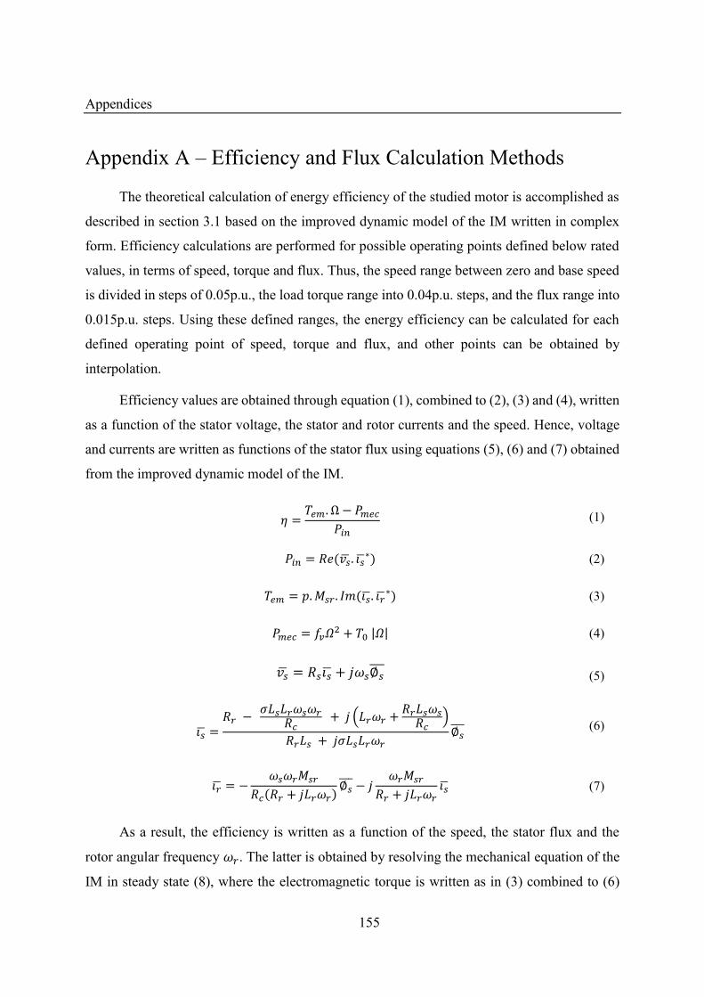
Appendices
155
Appendix A – Efficiency and Flux Calculation Methods
The theoretical calculation of energy efficiency of the studied motor is accomplished as
described in section 3.1 based on the improved dynamic model of the IM written in complex
form. Efficiency calculations are performed for possible operating points defined below rated
values, in terms of speed, torque and flux. Thus, the speed range between zero and base speed
is divided in steps of 0.05p.u., the load torque range into 0.04p.u. steps, and the flux range into
0.015p.u. steps. Using these defined ranges, the energy efficiency can be calculated for each
defined operating point of speed, torque and flux, and other points can be obtained by
interpolation.
Efficiency values are obtained through equation (1), combined to (2), (3) and (4), written
as a function of the stator voltage, the stator and rotor currents and the speed. Hence, voltage
and currents are written as functions of the stator flux using equations (5), (6) and (7) obtained
from the improved dynamic model of the IM.
� = .Ω −� (1)
� = . � ∗ (2)
= . . � . � ∗ (3)
= �� + |�| (4) = � + � ∅ (5)
� = − � � �
+ � + � + � � ∅ (6)
� = − � �+ � ∅ − �+ � � (7)
As a result, the efficiency is written as a function of the speed, the stator flux and the
rotor angular frequency � . The latter is obtained by resolving the mechanical equation of the
IM in steady state (8), where the electromagnetic torque is written as in (3) combined to (6)
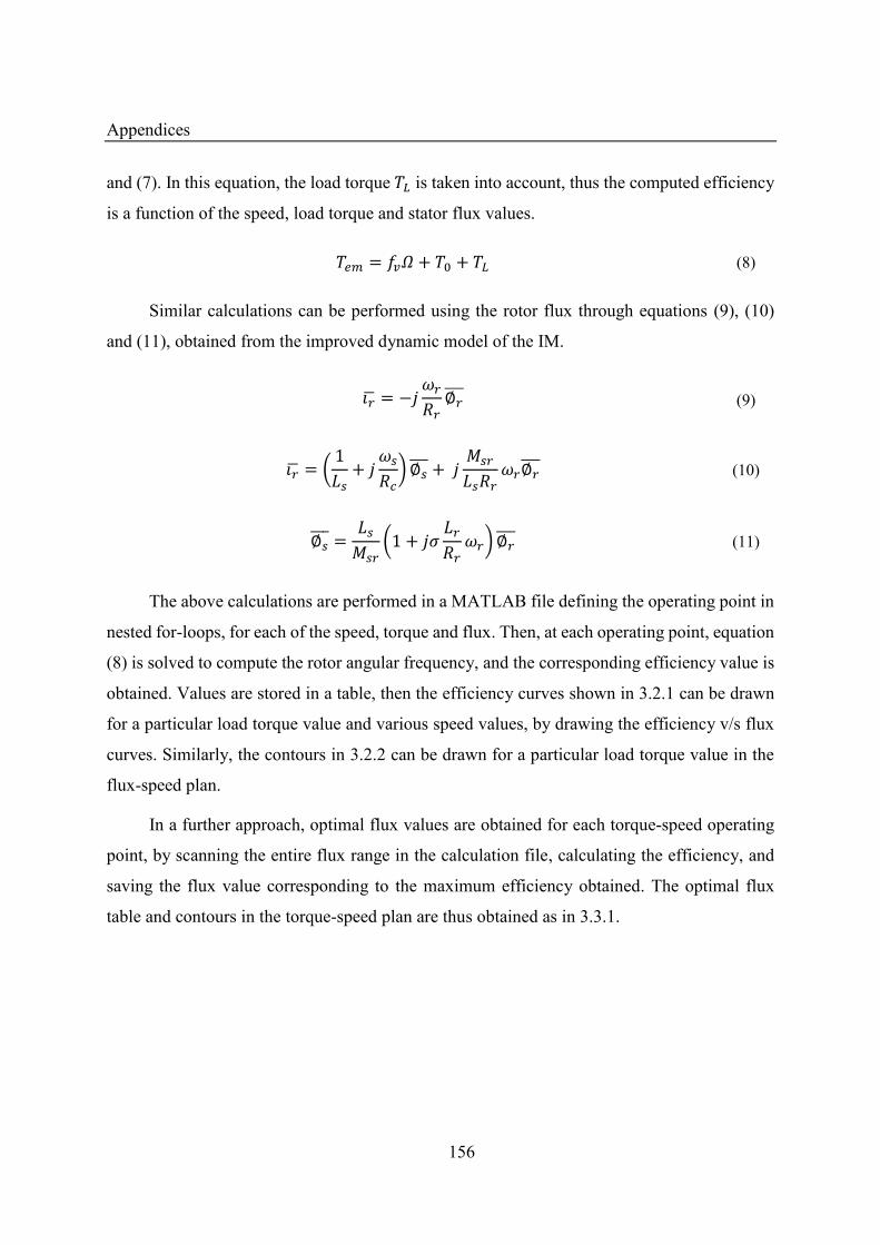
Appendices
156
and (7). In this equation, the load torque is taken into account, thus the computed efficiency
is a function of the speed, load torque and stator flux values. = �� + + (8)
Similar calculations can be performed using the rotor flux through equations (9), (10)
and (11), obtained from the improved dynamic model of the IM.
� = − � ∅ (9)
� = ( + � ) ∅ + � ∅ (10)
∅ = ( + � � ) ∅ (11)
The above calculations are performed in a MATLAB file defining the operating point in
nested for-loops, for each of the speed, torque and flux. Then, at each operating point, equation
(8) is solved to compute the rotor angular frequency, and the corresponding efficiency value is
obtained. Values are stored in a table, then the efficiency curves shown in 3.2.1 can be drawn
for a particular load torque value and various speed values, by drawing the efficiency v/s flux
curves. Similarly, the contours in 3.2.2 can be drawn for a particular load torque value in the
flux-speed plan.
In a further approach, optimal flux values are obtained for each torque-speed operating
point, by scanning the entire flux range in the calculation file, calculating the efficiency, and
saving the flux value corresponding to the maximum efficiency obtained. The optimal flux
table and contours in the torque-speed plan are thus obtained as in 3.3.1.
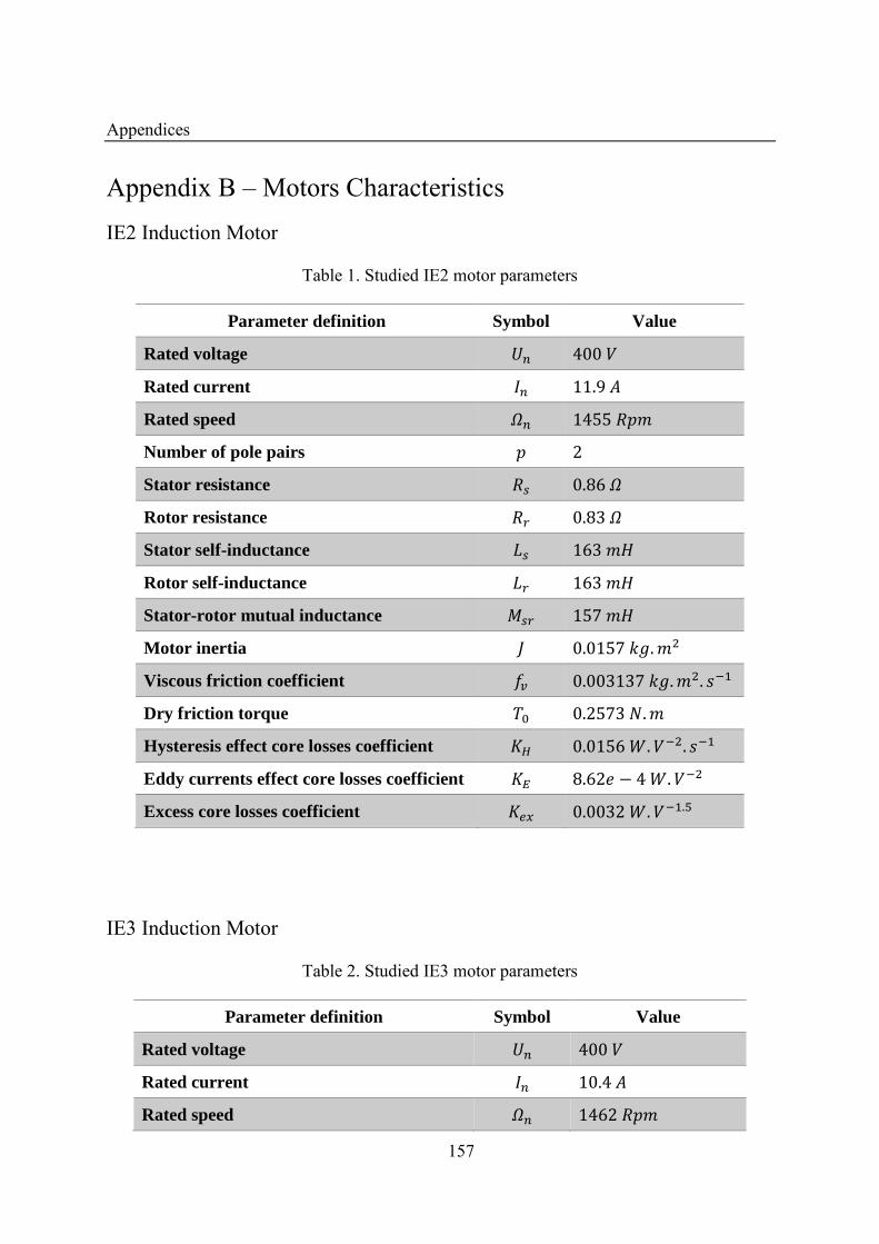
Appendices
157
Appendix B – Motors Characteristics IE2 Induction Motor
Table 1. Studied IE2 motor parameters
Parameter definition Symbol Value
Rated voltage
Rated current .
Rated speed �
Number of pole pairs
Stator resistance . �
Rotor resistance . �
Stator self-inductance
Rotor self-inductance
Stator-rotor mutual inductance
Motor inertia . .
Viscous friction coefficient � . . . −
Dry friction torque . .
Hysteresis effect core losses coefficient � . . − . −
Eddy currents effect core losses coefficient . − . −
Excess core losses coefficient � . . − .5
IE3 Induction Motor
Table 2. Studied IE3 motor parameters
Parameter definition Symbol Value
Rated voltage
Rated current .
Rated speed �
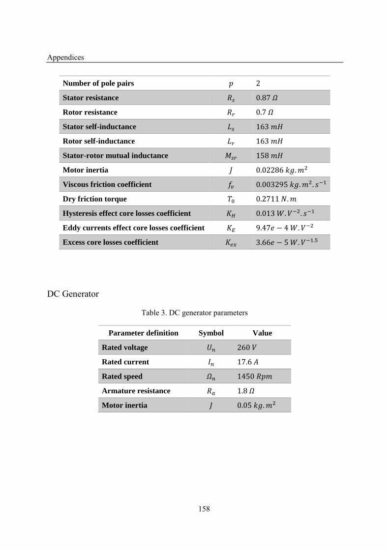
Appendices
158
Number of pole pairs
Stator resistance . �
Rotor resistance . �
Stator self-inductance
Rotor self-inductance
Stator-rotor mutual inductance
Motor inertia . .
Viscous friction coefficient � . . . −
Dry friction torque . .
Hysteresis effect core losses coefficient � . . − . −
Eddy currents effect core losses coefficient . − . −
Excess core losses coefficient � . − . − .5
DC Generator
Table 3. DC generator parameters
Parameter definition Symbol Value
Rated voltage
Rated current .
Rated speed �
Armature resistance . �
Motor inertia . .
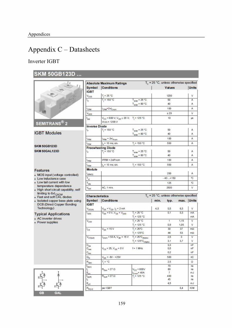
Appendices
159
Appendix C – Datasheets Inverter IGBT
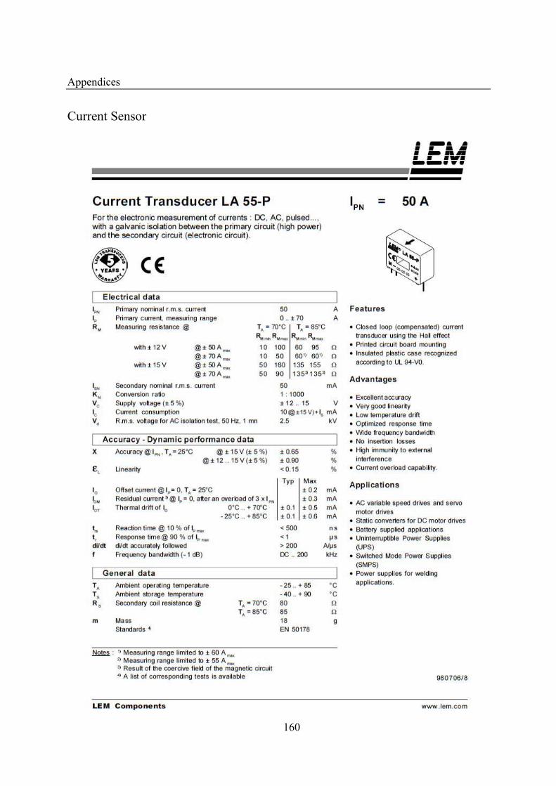
Appendices
160
Current Sensor
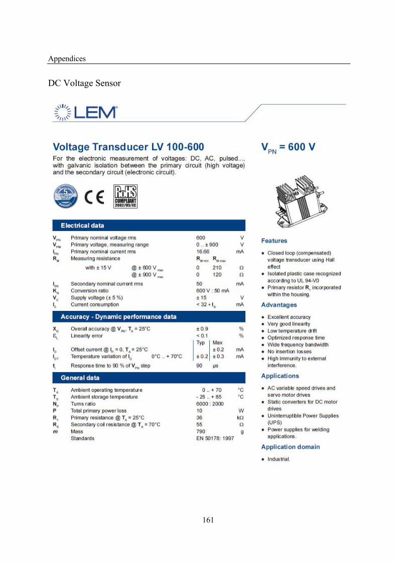
Appendices
161
DC Voltage Sensor
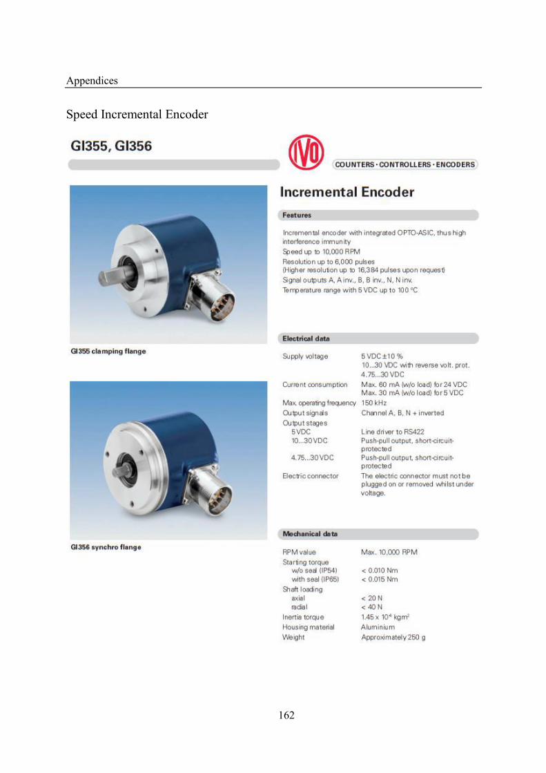
Appendices
162
Speed Incremental Encoder


