Embed Size (px)
Citation preview

This thesis has been submitted in fulfilment of the requirements for a postgraduate degree
(e.g. PhD, MPhil, DClinPsychol) at the University of Edinburgh. Please note the following
terms and conditions of use:
• This work is protected by copyright and other intellectual property rights, which are
retained by the thesis author, unless otherwise stated.
• A copy can be downloaded for personal non-commercial research or study, without
prior permission or charge.
• This thesis cannot be reproduced or quoted extensively from without first obtaining
permission in writing from the author.
• The content must not be changed in any way or sold commercially in any format or
medium without the formal permission of the author.
• When referring to this work, full bibliographic details including the author, title,
awarding institution and date of the thesis must be given.

Red squirrel habitat mapping using remote sensing
Silvia Flaherty
A thesis submitted in fulfilment of requirements for the degree of Doctor
of Philosophy
School of GeoSciences
University of Edinburgh
2012

i
Declaration
I hereby declared that this thesis is of my own composition, and that it contains no
material previously submitted for the award of any other degree. The work reported
in this thesis has been executed by myself, except where due acknowledgments is
made in the text.
Silvia Flaherty

ii
Abstract
The native Eurasian red squirrel is considered endangered in the UK and is under
strict legal protection. Long-term management of its habitat is a key goal of the UK
conservation strategy. Current selection criteria of reserves and subsequent
management mainly consider species composition and food availability. However,
there exists a critical gap in understanding and quantifying the relationship between
squirrel abundance, their habitat use and forest structural characteristics. This has
partly resulted from the limited availability of structural data along with cost-
efficient data collection methods. This study investigated the relationship between
squirrel feeding activity and structural characteristics of Scots pine forests. Field data
were collected from two study areas: Abernethy and Aberfoyle Forests. Canopy
closure, diameter at breast height, height and number of trees were measured in 56
plots. Abundance of squirrel feeding signs was used as an index of habitat use. A
GLM was used to model the response of cones stripped by squirrels in relation to the
field collected structural variables. Results show that forest structural characteristics
are significant predictors of feeding sign presence, with canopy closure, number of
trees and tree height explaining 43% of the variation in stripped cones. The GLM
was also implemented using LiDAR data to assess at wider scales the number of
cones stripped by squirrels. The use of remote sensing -in particular Light Detection
and Ranging (LiDAR) - enables cost efficient assessments of forest structure at large
scales and can be used to retrieve the three variables explored in this study; canopy
cover, tree height and number of trees, that relate to red squirrel feeding behaviour.
Correlation between field-predicted and LiDAR-predicted number of stripped cones
was performed to assess LiDAR-based model performance. LiDAR data acquired at
Aberfoyle and Abernethy Forests had different characteristics (in particular pulse
density), which influences the accuracy of LiDAR derived metrics. Therefore
correlations between field predicted and LiDAR predicted number of cones (LSC)
were assessed for each study area separately. Strong correlations (rs=0.59 for
Abernethy and 0.54 for Aberfoyle) suggest that LiDAR-based model performed
relatively well over the study areas. The LiDAR-based model was not expected to

iii
provide absolute numbers of cones stripped by squirrels but a relative measure of
habitat use. This can be interpreted as different levels of habitat suitability for red
squirrels. LiDAR-based GLM maps were classified into three levels of suitability:
unsuitable (LSC = 0), Low (LSC < 10) and Medium to High Suitability (LSC >=10).
These thresholds were defined based on expert knowledge. Such a classification of
habitat suitability allows for further differentiation of habitat quality for red squirrels
and therefore for a refined estimation of the carrying capacity that was used to
inform population viability analysis (PVA) at Abernethy Forest. PVA assists the
evaluation of the probability of a species population to become extinct over a
specified period of time, given a set of data on environmental conditions and species
characteristics. In this study, two scenarios were modelled in a PVA package
(VORTEX). For the first scenario (Basic) carrying capacity was calculated for the
whole forest, while for the second scenario (LiDAR) only Medium-to-High suitable
patches were considered. Results suggest a higher probability of extinction for the
LiDAR scenario (74%) than for the Basic scenario (55%). Overall the findings of this
study highlight 1) the importance of considering forest structure when managing
habitat for squirrel conservation and 2) the usefulness of LiDAR remote sensing as a
tool to assist red squirrel, and potentially other species, habitat management.

iv
Acknowledgments
My biggest thanks are reserved for my supervisors Dr Genevieve Patenaude, for her
support, patience and guidance throughout this project and Dr Peter Lurz, who very
kindly adopted me as his student and very patiently helped me understand the
squirrel world. I would also like to thank my co-supervisors Dr Tim Malthus and Dr
Iain Woodhouse for their advice.
Without funding from the University of Edinburgh and the Forestry Commission
Scotland this PhD would have not been possible. I would also like to acknowledge
the support of the NERC Airborne Research and Survey Facility for acquiring and
providing the LiDAR data. Thanks in particular to Mark Warren for his help with the
pre-processing of the data.
Special thanks to Dr Juan Suarez, Dr Rachael Gaulton, Dr Alasdair MacArthur, Chris
Place, Owen MacDonald, Dr Andrew Close and Dr Pablo Rosso for their advice in
different moments of this PhD. Thanks also to Stewart Snape, Juliet Robinson, Dr
Mel Tonkin, Jo Ellis, Andy Amphlett and all the individuals and organisations that
contributed to this research.
Field work was possible thanks to the funding provided by the People’s Trust for
Endangered Species. I would also like to thank Wayne Fitter, Xavier De Lamo,
Kushal Gurung and all the volunteers for their invaluable help and willingness to
work during the field seasons.
Finally, my warmest thanks are due to my mother and my brother for their love and
support, and to my friends, the ones in the UK and the ones overseas, for their love,
support and encouragement.

v
Table of Contents
Declaration.................................................................................................................... i
Abstract........................................................................................................................ ii
Acknowledgments ...................................................................................................... iv
Table of Contents .........................................................................................................v
CHAPTER 1 .................................................................................................................1
General Introduction ...................................................................................................1
1.1 Introduction .................................................................................................. 1
1.1.1 Grey squirrels versus red squirrels....................................................... 1
1.1.2 Squirrelpox virus.................................................................................. 4
1.1.3 Woodland cover ................................................................................... 5
1.1.4 Predation .............................................................................................. 6
1.2 Red squirrel habitat suitability ..................................................................... 6
1.2.1 Modelling habitat suitability for red squirrel in the UK ...................... 7
1.2.2 Red squirrel habitat preferences........................................................... 9
1.3 Forest management .................................................................................... 11
1.4 Red squirrels strongholds and forest structure ........................................... 13
1.5 Remote sensing for biodiversity and habitat mapping............................... 14
1.6 Thesis aims and scope................................................................................ 18
1.7 Thesis structure .......................................................................................... 19
The impact of forest-stand structure on red squirrel habitat use .........................21
2.1 Introduction ................................................................................................ 21
2.2 Methodology .............................................................................................. 24
2.2.1 Study area........................................................................................... 24
2.2.2 Stands selection and sampling strategy.............................................. 27
2.2.3 Data analysis ...................................................................................... 28
2.3 Results ........................................................................................................ 29
2.4 Discussion .................................................................................................. 34
CHAPTER 3 ...............................................................................................................37
LiDAR data processing for red squirrels habitat mapping ...................................37
3.1 Introduction ................................................................................................ 37
3.1.1 LiDAR remote sensing....................................................................... 37

vi
3.1.2 LiDAR data processing for red squirrel habitat mapping .................. 38
3.1.2.1 Canopy cover ................................................................................. 39
3.1.2.2 Individual tree delineation.............................................................. 40
3.1.2.3 Mean tree height............................................................................. 43
3.1.3 FUSION ............................................................................................. 45
3.2 Methodology .............................................................................................. 46
3.2.1 LiDAR data processing ...................................................................... 46
3.2.2 DTM and CHM.................................................................................. 47
3.2.3 Canopy Cover .................................................................................... 49
3.2.4 Individual trees................................................................................... 51
3.3 Results ........................................................................................................ 54
3.3.1 Digital terrain model .......................................................................... 54
3.3.2 Canopy Cover .................................................................................... 61
3.3.3 Number of trees.................................................................................. 62
3.3.3.1 Canopy height model approach...................................................... 62
3.3.3.2 Cloud of points approach ............................................................... 63
3.3.4 LiDAR 90th
and 95th
percentiles and mean tree height ...................... 67
3.4 Discussion .................................................................................................. 70
3.4.1 Digital Terrain Model ........................................................................ 70
3.4.2 Canopy Cover .................................................................................... 71
3.4.3 Individual tree delineation.................................................................. 73
3.4.4 LiDAR 90th
and 95th
percentiles as estimators of mean tree height... 75
CHAPTER 4 ...............................................................................................................77
GLM implementation using LiDAR derived explanatory variables.....................77
4.1 Introduction ................................................................................................ 77
4.2 Methodology .................................................................................................... 81
4.2.1 Study Areas ............................................................................................... 81
4.2.2 Field-based GLM validation .................................................................... 82
4.2.3 Implementation of GLM using LiDAR .................................................... 83
4.2.3.2 Raster file generation ......................................................................... 84
4.2.3.3 GLM implementation......................................................................... 87
4.2.3.4 Habitat suitability maps...................................................................... 88

vii
4.3 Results .............................................................................................................. 90
4.3.1 Field-based GLM validation ..................................................................... 90
4.3.2 Implementation of GLM using LiDAR .................................................... 90
4.3.2.1 Calibration of Aberfoyle number of trees ........................................ 93
4.3.2.2 Habitat suitability maps.................................................................. 93
4.4 Discussion .................................................................................................. 98
4.4.1 Field-based GLM ............................................................................... 98
4.4.2 LiDAR-based GLM ........................................................................... 99
CHAPTER 5 .............................................................................................................102
Using LiDAR derived habitat suitability data to model red squirrel population
viability......................................................................................................................102
5.1 Introduction .............................................................................................. 102
5.1.1 Population Viability Analysis .......................................................... 104
5.1.2 Modelling population viability......................................................... 105
5.1.3 Sensitivity analysis........................................................................... 106
5.1.4 Background ...................................................................................... 107
5.1.4.1 Case studies.................................................................................. 107
5.1.4.2 Comparison between PVA packages ........................................... 113
5.1.5 VORTEX ......................................................................................... 114
5.1.5.1 Input parameters........................................................................... 115
5.2 Methodology ............................................................................................ 117
5.2.1 Model validation .............................................................................. 117
5.2.1.1 Kidland Forest.............................................................................. 117
5.2.1.2 Model Input data .......................................................................... 118
5.2.2 Sensitivity analysis........................................................................... 122
5.2.3 Red squirrel population viability analysis at Abernethy Forest ....... 122
5.2.3.1 Abernethy Forest .......................................................................... 122
5.2.3.2 Model Input Data & Scenarios..................................................... 122
5.3 Results ...................................................................................................... 127
5.3.1 Model Validation ............................................................................. 127
5.3.2 Sensitivity analysis........................................................................... 128
5.3.3 Red squirrel population viability analysis at Abernethy Forest ....... 130

viii
5.4 Discussion ................................................................................................ 133
5.4.1 Model validation .............................................................................. 133
5.4.2 Sensitivity analysis........................................................................... 133
5.4.3 Red squirrel population viability analysis at Abernethy Forest ....... 134
5.4.5 The use of LiDAR remote sensing for PVA .................................... 136
CHAPTER 6 .............................................................................................................138
Discussion and conclusions......................................................................................138
6.1 Forest structure and red squirrel habitat preferences ............................... 138
6.2 The use of LiDAR remote sensing........................................................... 142
6.3 Transferability, repeatability and further applications of methods .......... 147
6.4 Contribution of research........................................................................... 148
6.5 Overall conclusions.................................................................................. 149
6.6 Key recommendations.............................................................................. 150
EPILOGUE...............................................................................................................151
REFERENCES.........................................................................................................152
APPENDIX A – Red squirrel sightings..................................................................163
APPENDIX B – LiDAR & field values- Tables.....................................................168
APPENDIX C – GLM validation – Tables ............................................................178
APPENDIX D – VORTEX predictions – Abernethy Forest................................181
APPENDIX E – Related publications ....................................................................182

1
CHAPTER 1
General Introduction
__________________________________________________________
1.1 Introduction
The red squirrel (Sciurus vulgaris) – the only squirrel species native to the UK- was
previously widespread all over England, Scotland and Wales (Gurnell, 1987; Lurz et
al., 1995; Bryce et al., 2005; Poulsom et al., 2005). Intensive tree felling in the 17th
and 18th centuries, causing habitat fragmentation and woodland loss, resulted in an
severe reduction in the number of red squirrels. More recently, the introduction of
grey squirrel (Sciurus carolinensis) from North America largely contributed to a
further decline in red squirrel populations in Britain. Nowadays, the grey squirrel has
replaced reds in most of England, Wales and Central Scotland (Lurz et. al., 1995).
The decline in red squirrel populations has lead to concern about the conservation
status of the species, which is now considered endangered, listed in the UK
Biodiversity Action Plan and under legal protection (Schedules 5 and 6 of the
Wildlife and Countryside Act 1981, Nature Conservation (Scotland) Act 2004; and
WANE Act 2011). Today, long-term management of red squirrel habitats is a key
goal of the UK Strategy for Red Squirrel Conservation (Bryce et al., 2005)
Although the grey squirrel is currently thought to be the major threat, disease (i.e.
squirrelpox virus) and habitat quality are also important factors affecting the future
of red squirrels in the UK (Gurnell et al., 2004; Rushton et al., 2006a). Conservation
efforts currently concentrate mainly in controlling grey squirrels and managing
woodlands to favour red squirrels (Forestry Commission, 2012; Poulsom et al., 2005;
Mackinlay & Patterson, 2011)
The following section provides an overview of the main factors (e.g. competition
with greys, squirrelpox virus) that currently threaten red squirrel survival in the UK.
Research and main findings on the species habitat preferences leading to current
habitat management strategy will also be reviewed.
1.1.1 Grey squirrels versus red squirrels
A great deal of research is dedicated to investigating the impact of exotic species
introduction on native species (Tompkins et. al., 2003). In the particular case of the

2
red squirrel in the UK, the introduction of the grey squirrel from North America has
largely contributed to a decrease in red squirrel populations in Britain. The largest
number of grey squirrel was introduced in 1889, although there is evidence that a
pair was brought to England in 1876. In Scotland, the grey squirrel was first
introduced in 1892, and in Ireland in 1913 (Middleton, 1930). Since its introduction,
the species has spread and replaced red squirrels in most of England, Wales as well
as Central and Southern Scotland (Lurz et. al., 1995; for red/grey squirrel distribution
maps refer to: Naturally Scottish - Red Squirrels, SNH, 2010, pp 4-5). This
phenomenon is not only limited to the UK but has also been observed in other
countries where grey squirrels have been introduced, such as Ireland and Italy
(Teangana et al., 2000; Lurz et al., 1995; Rushton et al., 2000; Gurnell et. al., 2004).
The mechanisms by which the greys are replacing reds are still being investigated
and a number of hypotheses have been proposed. The grey squirrel is native to mixed
forests rich in broadleaves in Eastern USA while the red squirrel is mainly adapted to
living in conifer forests (Gurnell, 1987). These differences partly explain the way
both species have evolved: grey squirrels are larger and heavier than reds and they
spend most of their time on the ground, feeding on fallen seeds. Meanwhile reds are
smaller and lighter and therefore can feed on cones in canopies, where they spend
most of their time (approximately 70%), unlike grey squirrels which spend only 14%
of their time in the canopy (Gurnell, 1987, Gurnell & Pepper, 1991). It must be
highlighted however, that this is a general trend only: red squirrels have been
observed to spend a larger amount of time feeding on the forest floor, while greys in
Hamsterley Forest, for example, have been seen to spend most of their time in the
canopy, where the food was more abundant (P.Lurz, pers. comm., 2012). The
adaptation of the two species to their different habitats is also evident in other aspects
of their ecology. For instance, grey squirrels appear more tolerant than reds to a toxic
substance present in acorn, which explains why red squirrel densities are lower in
deciduous forests dominated by oak (Quercus) trees (Lurz et. al., 1995; Kenward &
Hodder, 1998; Gurnell et. al., 2004). This observation is further supported by
Tompkins et al., (2003) who reported that in years of good acorn crops in Norfolk,
England, grey squirrel reach very high densities. This has consequences for reds, as
large populations of greys also feed on other tree seeds, such as hazel nuts (Corylus),
reducing in this way the red squirrel's source of food and thus, its survival (Tompkins
et al., 2003). It is worth emphasizing here that both squirrel species are capable of

3
surviving in both broadleaved and conifer forests (Gurnell, 1987). Yet, the densities
at which they live in the two different habitat types varies: while both grey and red
squirrel densities fluctuate between 0.4 to 1.2 animals per ha in conifer forests, grey
squirrel densities reach much higher values (2 to 8 per ha) in broadleaved forests
(Gurnell & Pepper, 1991). This explains and highlights the importance of conifer
forests in relation to red squirrel conservation in the UK. This will be discussed in
more detail later in this chapter.
Mechanisms of competition between red and grey squirrel seem to be more subtle
than direct aggressive interaction between the two species (Gurnell, 1987). Gurnell
et. al. (2004) conducted a study in Hamsterley Forest, England (conifer forest) and
Borgo Cornalese, Italy (mixed broadleaves and conifers). They compared two red-
only with two red-grey sites, and their results indicate that the presence of grey
squirrels negatively influence red squirrel in a number of ways. In habitats where
reds coexist with greys, they observed a reduction in: red squirrel body mass;
juvenile recruitment, number of females producing a second litter and summer
breeding. Previous research by Wauters et al. (2002) reported that grey squirrels
coexisting with reds were observed to pilfer their food catches, and as suggested by
the authors, this probably is also the case in the UK. Red squirrels depend on seeds
hoarded in autumn as a source of food for the following winter and spring, and a
reduction in the amount of food recovered would reduce energy intake, and
potentially lead to a reduced body mass in spring and the consequent reduction in
fertility and reproduction (Wauters et al., 2002). In terms of foraging behaviour,
earlier studies by Wauters et al. (2001) conducted in two sites (red-only and red-
grey) in Italy suggested that red squirrel feeding activity (i.e. time spent searching for
food, time spent foraging) and food choice do not differ substantially between red
squirrels that coexist with greys and those that do not share their habitat with greys.
However, this does not match results from a study carried out in the Goathorn
Peninsula, Dorset, where 14 red squirrels were released in a conifer forest dominated
by Scots pine and with some oak and chestnut (Castanea), and where grey squirrels
were also present (grey squirrel density is not reported, Kenward & Hodder, 1998).
Out of the 14 initial squirrels, 11 died over the first 3 months, the majority due to
predation, but a minority died of diseases that typically affect stressed individuals
(adrenal hypertrophy, septicaemia, enteritis). The 3 red squirrels that survived the
longest and settled among the greys had problems foraging (i.e. as indicated by an
increase in their core areas) despite an abundance of food. These results suggest that

4
grey squirrel could potentially interfere with red squirrel foraging behaviour
(Kenward & Hodder, 1998). Some researchers have argued that the detrimental
effects on red squirrel populations of competition with greys is density dependant
and measurable effects increase with increasing number of grey squirrels (Bryce et.
al., 2005; Wauters et al., 2002).
The findings summarised in this section show that competition between reds and
greys is a major reason for the decreasing number of red squirrels in the UK.
However, other factors such as disease have been investigated and are thought to
play an important role in population decline (Tompkins et al., 2003). Indeed,
decrease in red squirrel population was observed in the past, before grey squirrel was
introduced, and this was linked to disease (Middleton, 1930).
1.1.2 Squirrelpox virus
Previously known as parapox virus, squirrelpox virus (SQPV) is caused by a
poxvirus and it is thought to be one of the reasons for the red squirrel population
decline in the UK, in particular in England and Wales. More recently (2005), the first
four cases of SQPV were detected in Scotland causing great concern, as Scotland is
home to approximately 75% of the remaining red squirrel population in Britain
(McInnes et al., 2009).
It has been suggested that while SQPV severely affects and kills red squirrels,
infected grey squirrels carry the virus but do not become ill thus acting as reservoir
host for the virus (Rushton et. al., 2000; Tompkins et. al., 2003; McInnes et al.,
2009). Recent research by Fiegna (2011) reported that grey squirrels infected with
SQPV nevertheless presented skin lesions (i.e. oral skin and lips). Their results also
confirmed that skin lesions in grey squirrels were less severe than those in infected
red squirrels.
The apparent severity in the way the disease affects red squirrels suggests that most
individuals are likely to die before they can spread it to other populations, which
reinforces the assumption that the virus is spread by infected yet asymptomatic grey
squirrels (Rushton et. al., 2000).
Direct contact between greys and reds rarely occurs and a number of possible
transmission routes have been suggested. These include: anal dragging, saliva or
scent marks left on branches by the two squirrels’ species. This constitutes part of
their olfactory communicational behaviour (Gurnell, 1987, Rushton et al. 2000).

5
Feeders used to provide red squirrels with supplementary food can also help to
spread the virus, as well as trapping or any management that can potentially attract
both red and grey squirrels to the same focal points (Bruemmer et al., 2010). A study
by Atkin et al. (2010) suggested that fleas could potentially be a transmission vector
for SQPV.
Since grey squirrels densities are higher in broadleaf woodlands, this habitat type
would potentially host more grey squirrels and therefore increase the possibility of
encounters and thus virus transmission (Rushton et. al., 2000). There are also other
considerations for managing conservation areas: increasing habitat connectivity may
also increase the risk of virus transmission and habitat de-fragmentation, usually
thought to be beneficial (i.e. to avoid isolation of populations), can be harmful in this
context (Tompkins et. al., 2003, Rushton et. al., 2000).
In large, non-endangered species populations, diseases play a regulatory role
(Rushton et. al., 2000). However, in the case of the red squirrel in the UK, SQPV
coupled with the negative effects of competition with greys described above is
speeding up both red squirrel decline and its ecological replacement by the greys
(Tompkins et al.., 2003; Rushton et al., 2006a). More in-depth reviews of SQPV can
be found in Rushton et. al., 2000; Tompkins et. al., 2003 and McInnes et al., 2009.
1.1.3 Woodland cover
Habitat loss and modification are among the most important reasons why species
become endangered. In many countries of northern Europe, intensive management of
forests has affected biodiversity in a negative way. As a consequence, species whose
habitats are natural forests have largely declined (Manton et. al., 2005).
In the UK, forests went from covering 75% of the land surface area in the post-
glacial period to approximately 5% at the start of the 20th century (Watts et. al.,
2005).
The loss of woodland and the fragmentation of forests reduced the amount of
available habitat and increased the isolation of populations. This had serious
consequences for the country's biodiversity. Nowadays, 15% of the species listed in
the UK Biodiversity Action Plan inhabit forests (Watts et. al., 2005).
In the case of the red squirrel, populations throughout the country were particularly
affected by the felling of tree species such as Scots pine (Pinus sylvestris) and
Norway spruce (Picea abies) and their replacement by sitka spruce (Picea sitchensis)
6
for commercial reasons (i.e. timber production) during the first half of the 20th
century (Mackinlay & Patterson, 2011).
In recent years, more biodiversity-friendly forest policies have been implemented.
Nowadays, 11% of the UK is covered by forest (Watts et al., 2005). In Scotland,
woodland cover increased up to 17% by 2006 as part of a governmental strategy
aiming to reach 25% woodland cover by the end of the century (Scottish Forest
Strategy 2006). This increase in woodland cover is expected to help reverse the loss
of biodiversity (Watts et. al., 2005). However, priority species such as the red
squirrel require targeted and informed habitat management for their conservation.
More information on current research on landscape ecology and biodiversity in the
UK can be found in Watts et al. (2005) and Watts et al. (2007).
1.1.4 Predation
Predation is one of the factors which can potentially influence red squirrel numbers
in the UK. Main predators of red squirrel are goshawk (Accipiter gentiles), buzzard
(Buteo buteo) and the pine marten (Martes martes) (Halliwell, 1997). Other predators
include the red fox (Vulpes vulpes) and cats (Felis sp); Bosch & Lurz, 2012).
Two studies investigated the predation of red squirrel by goshawk in Kielder Forest
(Petty et al., 2003) and the pine martens in Ross-shire (Halliwell, 1997). Pine
martens may prey on squirrels if other small mammals are not available, but in
general, red squirrels are only a small proportion of marten diet. Furthermore, pine
marten would also prey on grey squirrels (Bosch & Lurz, 2012).
In terms of predation of red squirrel by buzzards, a study carried out in Moray,
Scotland (and cited in Halliwell, 1997), stated that 22% of remains found at buzzard
nests were red squirrels.
Researchers arrived to similar conclusions: predation in general seems unlikely to
cause the extinction of the species (Halliwell, 1997; Petty et al., 2003). Yet, given the
low densities of red squirrel due to other factors discussed previously (i.e.
competition with greys, squirrelpox virus, habitat degradation) predation is assumed
to accelerate the decline of the species populations (Halliwell, 1997).
1.2 Red squirrel habitat suitability
In order to design and implement effective management strategies, it is first
necessary to assess red squirrel habitat requirements. A number of studies have been

7
carried out to better understand red squirrel preferences in the UK. A summary of the
most relevant findings is provided in the following sections. The first section
provides a review of red squirrel habitat modelling studies, while the second section
summarises results from studies investigating the species' preferences based on red
squirrel field surveys (i.e. live-trapping, radio tracking).
1.2.1 Modelling habitat suitability for red squirrel in the UK
A number of studies have used modelling approaches to assess red squirrel habitat
suitability and investigate the species preferences in UK forests.
Lurz et al. (1995) used a general linear model (GLM) to predict the number of
squirrels in different habitat types in Spadeadam Forest, England. Squirrel densities
were estimated based on live-trapping for 27 sites over a period of 3 years (1992 to
1994). The size of each area ranged from 21 to 60ha. The GLM was used to assess
the relationship between squirrel densities and three independent variables: woodland
area; proportion of Norwary spruce (NS) and Lodgepole pine (Pinus contorta, LP)
relative to sitka spruce (SS; proportion of NS and LP = (NS+LP)/SP) and
presence/absence of Norway spruce. Their results suggest that red squirrel densities
increase when woodland area increases. Furthermore, the number of squirrels also
increased with the presence of Norway spruce and with a higher proportion of
Norway spruce and Lodgepole pine relative to sitka spruce: keeping the proportion
of Lodgepole pine constant, red squirrel density per ha ranged from 0.02 when all the
spruce-area was planted with sitka spruce, to 1.95 when 80% of the spruce-area was
planted with Norway spruce. These results highlight the low suitability of sitka
spruce for red squirrel in the UK and the importance of mixed conifers composition
for red squirrel conservation.
Commercial forests in the UK consist predominantly of compartments and sub-
compartments (i.e. management units), where each sub-compartment is composed of
a particular tree species (and age). In Thetford Forest, England, the size of each sub-
compartment ranges from 1 to 40ha. Using a GIS approach, Gurnell et al. (2002)
investigated the suitability of the forest by analysing the suitability of sub-
compartments. Thetford Forest consists mainly of Scots pine and Corsican pine
(Pinus nigra), 10% of broadleaves and 5 % of other conifers. Based on live-trapping
and published information, they assessed red squirrel habitat preferences within the
forest, and assigned 3 habitat suitability levels: low, medium and high, where

8
medium and high suitability sub-compartments consisted of tree species of an age
that could support medium to high density of squirrels respectively; and low
suitability sub-compartments (i.e. felled sub-compartments or plantations too young
to produce food) were assumed not to support resident populations of squirrels.
One scenario combined sub-compartments of medium to high suitability with
different linking distances (0, 50, 100 and 200m) to estimate different sizes of total
suitable area (i.e. suitable sub-compartments linked together) for the whole forest.
Another scenario estimated total suitable area at 5 years intervals (from 1995 to
2015) keeping linking distance constant (100 m) and considering felling and
restocking plans for the forest. Results from this study showed little or not
differences in the total size of suitable area of the reserve when combined with the
different linking distances. This is probably due to sub-compartments being
proportionally too large relative to the linking distances. Linking distances between
suitable patches are important as red squirrels would move across patches of low
suitability, provided their size does not exceed their home range (approximately 3 to
20 ha in conifer forests; Bosh & Lurz, 2012). This indicates the need for more
research in this area to identify realistic linking distances. When considering felling
and restocking plans, total suitable area increased from 39% (of the total woodland
area) in 1995 to 67% in 2015, suggesting that management plans for the forest would
increase the suitability for red squirrel. However, the results also suggested that if
sitka spruce was planted instead of Corsican pine, the total suitable area would drop
to 24% in 2015. Habitat preferences in terms of species composition and age
resulting from red squirrel live-trapping carried out in this project are summarized in
the next section.
The effects of forest management on red squirrel population in Kidland Forest, UK
(55° 25’ N; 2° 10’ W), were explored by Lurz et al. (2003). Kidland Forest is a red
squirrel reserve dominated by sitka spruce, with small proportions of Lodgepole
pine, Scots pine and Larch (Larix). At the time the study was carried out, no grey
squirrels were present in the forest. However, plans to restore biodiversity in the
forest included re-planting 15 ha of oak, which could encourage grey squirrel
incursion. In order to model the effects of felling plans for the forest and potential
grey squirrel incursion, Lurz et al. (2003) used a spatially explicit population
dynamics model. The first component of the model worked on a GIS platform
(GRASS) and incorporated stock map data, future planting, felling plans and seed

9
crops patterns (based on tree species). The second component of the model used life-
history data to model red and grey squirrel population dynamics and viability based
on species composition, tree age, felling/restocking plans and seed production
patterns. All forest compartments that contained trees mature enough to produce
seeds were considered suitable habitat. To model the oak-planting scenario, it was
assumed that a small population of 20 grey squirrels was already present in the
forest. Dispersal was modelled once a year, and grey squirrels were allowed to
disperse to compartments where reds were present. Results suggested that poor sitka
spruce seed crops in combination with felling could potentially lead to the extinction
of red squirrels in Kidland Forest by 2012. Furthermore, in a mature-oak scenario,
grey squirrel population could potentially increase to an average of 80 individuals by
2050. These results illustrate the need to carefully assess management strategies and
objectives, in particular in forests where red squirrel conservation is a priority.
Furthermore, priorities for red squirrel conservation and management may have to be
set at the landscape scale to accommodate different priorities and to reduce potential
conflicts e.g. management of red squirrels and planting of ancient woodland sites
with native oak species.
1.2.2 Red squirrel habitat preferences
While arboreal squirrels live on a variety of different types of food (buds, tree
flowers, fungi, berries), tree seeds remain their main diet. Hence squirrel densities
have been observed to vary annually along with variations in tree seed production
(Gurnell, 1987; Lurz et. al., 1995). Furthermore, squirrels are known to prefer seeds
with a high nutrient content (Gurnell, 1987). Given that different tree species
produce seeds with different nutrient content (Grönwall, 1982), tree species
composition and age (i.e. trees mature enough to produce food) are important factors
determining red squirrel habitat preferences (Lurz et al., 1995).
Studies carried out elsewhere (i.e. Belgium, Sweden and Finland) showed a strong
preference of red squirrels for pine and spruce seeds (Lurz et al., 1995). This is
supported by results from a number of studies carried out in the UK. Bryce et. al.
(2005) investigated tree species preferred by red squirrel in two forests in the UK:
Clocaenog Forest in North Wales and Craigvinean Forest in Perthshire, Scotland. In
this study, red squirrels were observed to select Norway spruce, Scots pine, Douglas
fir (Pseudotsuga) and larch over sitka spruce. This supports results from the
modelling studies discussed above, where model outputs suggested that red squirrel

10
population would increase if a proportion of sitka spruce was replaced by Norway
spruce in Spadeadam Forest, England (Lurz et al., 1995).
In terms of pine species, the study by Gurnell et al., (2002) showed that red squirrels
preferred Scots pine to Corsica pine in Thetford Forest, England.
Lurz et al. (1995) compiled data from previous studies that reported densities of red
squirrel per ha for different tree species in Northern Europe (i.e. England, Scotland,
Russia, Belgium and Sweden). Observed densities were based on studies which had
assessed trees selected by squirrels using feeding transects and live-trapping
sampling techniques. A summary of their results is provided below:
• Pure Scots pine stands support higher densities of red squirrels than any other
pure conifer species (0.33 to 0.8 red sq/ha)
• Plantations of pure sitka spruce support very low red squirrel population
densities (near 0 red squirrels/ha)
• The combination of sitka spruce (SS) with Norway spruce (NS) and/or
Lodgepole pine (LP) considerably improves habitat quality and increases carrying
capacity (e.g. 0.21 red sq/ha for SS+NS; 0.35 red sq/ha for SS+NS+LP).
• The highest red squirrel carrying capacity was observed with the combination
of Scots pine + Corsican pine + larch (1.01 to 1.41 red sq/ha)
Scots pine is one of the tree species most preferred by red squirrels in the UK
because they provide high nutrient content seeds and good cover (Lurz et al., 1995;
Gurnell et al., 2002). On the other hand, sitka spruce is less suitable for red squirrel
as it offers a less reliable (i.e. less frequent and abundant) food supply (Gurnell &
Pepper, 1991). It is important to highlight that most conifer species will produce a
mast crop (i.e. large cone crop) every 3 to 5 years, usually followed by a poor cone
crop year. This cycle is different for different tree species, and therefore, the number
of tree species present in a forest is important to ensure a continuous food supply for
red squirrels (Gurnell, 1987).
The age at which trees start and stop producing food is a crucial factor when
considering habitat suitability for squirrels. The study carried out by Gurnell et al.
(2002) in Thetford Forest showed that red squirrels preferred Scot pine younger than
49 year-old and Corsican pine between 25 and 34 year-old. Squirrels also preferred
Scots pine to Corsican pine as the former has its first good seed crop 10 to 15 years
earlier than Corsican pine. Furthermore, there is evidence of high numbers of red

11
squirrel being present in the reserve between 1950 and 1960 when Scots pine planted
in Thetford forest reached this favourable coning age (Gurnell et. al., 2002).
It can therefore be concluded that a range of conifer species and tree ages is
necessary to ensure food supply for red squirrel.
1.3 Forest management
The main reason for the continuous decline of the red squirrel in the UK is the
introduction of the grey squirrel. However, controlling grey squirrel might not be
feasible in the long term and therefore conserving red squirrel might strongly depend
on managing forests in a way that favours reds without encouraging greys (Gurnell et
al., 2002).
Based on the factors that currently threaten red squirrel survival in the UK (i.e. grey
squirrel, disease) and on the research carried out in the UK to investigate red squirrel
preferences in terms of species composition and age (discussed earlier in this
chapter) several management recommendations have been suggested by a number of
researchers, which are summarized below:
• The main driver for squirrel populations is food availability so any habitat
management intended to benefit habitat suitability for red squirrels should
contemplate diversification of conifer species and tree ages that would ensure
continuous supply of food for red squirrels (Lurz et al., 1995; Gurnell et al., 2002;
Bryce et. al., 2005).
• Large conifer forests (e.g. > 2000 ha) may represent an advantage for red
squirrels and may help to reduce competition for food with greys. (Lurz et al., 1995;
Gurnell et al., 2002; Bryce et. al., 2005).
• In the UK, grey squirrels exhibit a strong preference for acorns. Thus, conifer
forests with some oaks around are particularly vulnerable to grey squirrel invasion.
The inclusion of oaks needs to be carefully considered and, if possible, avoided in
forests managed for red squirrel conservation (Lurz et. al., 1995).
• The proportion of large-seeded broadleaves (not only oak but also chestnut,
beech ( Fagus) and hazel) should be minimised in mainland forests managed for red

12
squirrel conservation. Broadleaves scattered throughout a woodland might be more
detrimental (i.e. would encourage grey squirrels throughout the forest) than an
isolated cluster of these trees. (Bryce et. al., 2005).
• A buffer (1 to 3 km) might help reduce grey squirrel incursion. Small-seeded
broadleaves could be planted in those buffer areas (Bryce et. al., 2005).
• Native Scots pine seems to support higher densities of red squirrels than
Lodgepole pine and therefore it should be given preference (Lurz et. al., 1995).
Furthermore, Scots pine produce cones more regularly than Norway spruce. Thus,
some stands of Scots pine combined with Norway spruce would considerably
improve habitat suitability for red squirrel by ensuring food supply (Bryce et. al.,
2005).
• The presence of Norway spruce in stands of sitka spruce would be beneficial
for red squirrels as it considerably increases food supply (Lurz et al., 1995; Bryce et.
al., 2005).
• Current plans to expand and restore native woodlands in the UK need special
consideration. Linking existing forests may be beneficial for red squirrel as it would
allow dispersal and increase food availability. However, habitat management to
reduce red squirrel mortality due to squirrelpox infection needs to be also
contemplated. Keeping red squirrel populations in a relatively fragmented state
would help avoid virus transmission between individuals of the same species, while
maintaining red squirrel away from the greys would help to avoid both invasions by
greys and virus transmission. Both these cases lead to the conclusion that developing
forest networks need to be carefully considered (Poulsom et. al., 2005).
• Plans to restore native broadleaves need careful consideration, particularly in
areas designed for red squirrel conservation (Gurnell & Pepper 1993; Reynolds &
Bentley, 2001).
• Regarding felling and thinning operations, the study carried out in Clocaenog
Forest shows that squirrels leave their home ranges when thinning operations are
taking place but they stay nearby (200 m) and return afterwards. However, since it is

13
also known that good seed crops are important for red squirrels, avoiding felling in
good seed years would be beneficial (Bryce et. al., 2005).
• In order to maximise seed production, aspects such as fringe planting and
woodland irregular shapes to increase periphery need also be considered (Gurnell,
1987; Pepper & Paterson, 2001)
1.4 Red squirrels strongholds and forest structure
As part of the Scottish Government strategy for red squirrel conservation, 18 selected
sites or strongholds have been selected. The main aim of these strongholds is to
provide a refuge for long-term conservation of red squirrels in case grey squirrels
continue to spread. These strongholds were identified using Geographic Information
System (GIS), and the criteria used to select these sites were mainly based on the
absence/presence of red and grey squirrel in or near the site, the proportion of
broadleaves found and an assessment of conflict with other conservation objectives.
For an in-depth description of the selection process, the selection criteria, the list of
proposed strongholds and maps refer to Red squirrel strongholds (Forestry
Commission, 2009).
Habitat management for red squirrel conservation in these woodlands will be a
priority and will require an informed strategy. The importance of tree species
composition and food availability for squirrel abundance has been discussed early in
this chapter. However, a suitable place where a species can live should not only
entail food availability or the distribution of suitable nesting sites but it should also
present reduced risks of predation and limited competition (Gurnell, 1987; Gurnell et
al., 2002).
With respect to the red squirrel in the UK, a study carried out by Gurnell et al. (2002)
in Thetford Forest, England, showed that old stands of Scots pine that had been
subjected to intensive thinning were avoided by red squirrels despite the presence of
food. After late or final thinning is carried out in old stands, gaps among trees
become too large for the squirrels to move (Gurnell et al., 2002). This suggests that
even when food is present, other factors shape red squirrel preferences in terms of
habitat and that further research is necessary to understand and quantify the
relationship between red squirrel habitat use and forest structural factors such as
canopy connectivity, tree densities and height heterogeneity. The relationship

14
between vegetation structure and birds or small mammal distribution has been
investigated and a review of relevant literature is provided in Chapter 2. However,
evaluating and monitoring vegetation structure at the stand level is expensive and
time consuming. This highlights the need for research into methods that can extract
and utilise structural data to derive habitat suitability information over large forest
areas.
1.5 Remote sensing for biodiversity and habitat mapping
In recent years, there has been an increasing need for mapping habitat and
monitoring wildlife over large areas. Traditional methods of field data collection are
expensive and time consuming, and therefore, advances in technology such as
Geographical Information Systems (GIS) and remote sensing have become widely
used (McClain et. al., 2000). Both remote sensing and analytical GIS have proven to
be powerful tools for habitat mapping when time and budgets are limited (Weiers et.
al., 2004).
The list of studies that have used remotely sensed data to assess biodiversity and/or
to map habitat quality is long and it would be impossible to review all of them here.
Instead, a summary of the main and most used approaches is provided, and their
advantages and disadvantages are discussed. Table 1.1 provides some additional
examples.
Remotely sensed data have mainly been used to assess biodiversity and species
distribution by creating land-cover maps which represent species habitats (i.e.
forests, grasslands, wetlands). The combination of species habitat requirement and
land-cover maps allows for the assessment of, for example, potential species
presence or richness (Turner et al., 2003).
Visual interpretation of aerial photographs is probably one of the first remote sensing
methods used to assess species habitat. When performed by highly skilled
interpreters, visual interpretation of aerial photograph is very valuable and allows the
generation of accurate land-cover/land-use maps, detection of gaps, assessment of
habitat fragmentation and estimation of canopy cover. However, the manual nature
of the method makes it highly time consuming and only feasible when applied to
small areas (McDermid et al., 2005).
Multispectral satellite remote sensing such as LANDSAT TM or ETM + (6/7
spectral bands, 30m spatial resolution, see Table 1.1) provided an alternative to map

15
land-cover over large areas. Land-cover classification has been the object of a great
deal of research and several classification techniques have been developed. An in-
depth review of image classification can be found in Mather, 2004 or Lillesand,
Kiefer & Chipman, 2004. Satellite imagery classification provides land-cover maps
that can be integrated into a GIS along with other ancillary data (i.e. topography) to
assess, for example, habitat suitability for a particular species (McClain and Porter,
2000). Gaps and habitat fragmentation can also be detected as long as they cover
several pixels (McDermid et al., 2005).Although widely used and providing
relatively accurate and easy to understand outputs, land-cover maps generated from
multispectral LANDSAT TM/ETM+ data can be too coarse, lack detail or simply be
unable to discriminate classes (i.e. vegetation types) due to the limited spatial or
spectral resolution of multispectral data (McDermid et al., 2005).
Hyperspectral remote sensing is a relatively new technology that can improve land-
cover classification and therefore species habitat assessment. Satellite hyperspectral
detects reflected radiation across a continuous spectrum usually covering a minimum
of 100 spectral bands (Turner et al., 2003). This fine spectral resolution allows for
finer discrimination of land-cover types, in particular those related with vegetation
(i.e. tree species) improving in this way the assessment of the relationship between
species and habitat type (Turner et al., 2003). However, hyperspectral data can be
expensive and requires expertise to perform the pre-processing of the data, in
particular to remove atmospheric interference.
On the other hand, high spatial resolution remotely sensed data, such as IKONOS or
QuickBird, typically provide 4-band multispectral imagery with a spatial resolution
of approximately 2-3m, and a panchromatic band with a spatial resolution of around
1 m (see Table 1.1). These data allow the identification of individual features, for
example trees (Gougeon and Leckie, 2006). Although there is still a need for more
research in this subject, high spatial resolution data also allows for direct detection
and monitoring of species such as large marine mammals (i.e. whales) in Roatan
Island, Honduras (Abileah, 2001). Due to a limited spectral resolution, high spatial
resolution data offers little advantages in terms of land-cover mapping, but can
improve habitat mapping by, for example, providing accurate delineation of
individual trees, gaps and canopy cover (Turner et al., 2003).
Data fusion and synergistic use of remote sensing data involve the combination of
multi-source remote sensing data. This provides an opportunity to complement data
with different characteristics and obtain more reliable results (Wang et al., 2009). A

16
good example of data fusion would be the combination of data from hyperspectral
sensors with high spatial resolution data, which would allow for more detailed
description –in terms of both spectral and spatial resolution- of the area being
observed.
It is important to highlight that in all cases remotely sensed data should be validated
against field data to assess its accuracy (McDermid et al., 2005).
To the author’s knowledge, no peer-reviewed studies have used -or acknowledged
the use of- remotely sensed data to assist habitat quality assessment for red squirrel
in the UK. In most studies that have assessed or modelled habitat suitability for red
squirrel, land cover information and tree species composition have been obtained
from the National Inventory of Woodlands and Trees (NIWT; e.g. Poulsom et al.,
2005) and forest stock maps (e.g. Lurz et al., 1995; Gurnell et al., 2002).
Two studies by postgraduate students at the University of Edinburgh have used
remote sensing to map aspects of red squirrel habitat quality. Cristina García
(unpublished work, 2006) used high spatial resolution data (QuickBird imagery) to
map tree species composition at Kielder Forest, England. Tree species maps were
incorporated into a GIS system to identify suitable habitat for red squirrel based
solely on tree species composition and age (extracted from forest stock maps); while
Xavier de Lamo (unpublished work, 2010) used medium-spatial resolution
multispectral data (IRS-P6, 4 spectral bands, 23 m spatial resolution) to map canopy
closure in Aberfoyle Forest, Scotland, as a potential predictor of red squirrel
presence. A strong correlation (rs= 0.72) was found between field measured canopy
closure and Normalised Difference Vegetation Index (NDVI) which illustrates the
potential of remote sensing to extract one forest parameter (canopy closure)
potentially related to red squirrel habitat preferences. Results from these studies are
not conclusive and therefore they only provide an example of potential uses of
remote sensing to assist red squirrel habitat management
One limitation that all passive (i.e. optical) remote sensing data have in common is
the incapability to successfully characterize and describe vertical forest structure.
Active remote sensing, in particular LiDAR, can be used to directly measure
structural characteristics of forest stands such as canopy cover, canopy height and
height variability (Bradbury et. al., 2005; Turner et al., 2003).
This section has provided an overview of the most common applications of optical
remote sensing to habitat suitability mapping and biodiversity assessment. More in
depth reviews can be found in Turner et al., 2003; McDermid et al., 2005; Wang et

17
al., 2009 and Singh et al., 2010. Furthermore, a description of LiDAR remote
sensing and a detailed review of its use for species habitat mapping can be found in
Chapters 3 and Chapter 4 respectively.

18
Table 1.1: Literature examples showing some of the applications of remote sensing to
habitat mapping
Application Sensor (data type)
Resolution (spectral/spatial)
Species Reference
Land-cover, visual
interpretation
Aerial photograph
1:10000 Iberian lynx (Lynx pardinus)
Palma et al.., 1999
Land-cover classification
LANDSAT TM & ETM+ (passive)
6 spectral bands 0.45 – 2.35 µm/
30m Panchromatic
0.52-0.9 µm/15 m
Giant panda (Ailuropoda
melanoleuca)
Jian et al., 2011
Land-cover classification, multi-temporal
(change detection)
QuickBird (passive)
4 spectral bands 0.45-0.90 µm/
2.6 – 2.8m Panchromatic
0.445-0.90 µm/ 0.6 -0.7 m
Littoral vegetation
Heblinski, et al..; 2011
Individual items detection
(data fusion)
Ikonos (passive)
4 spectral bands 0.445 - 0.853 µm/
4m Panchromatic 0.45–0.90 µm/
0.8m
Marine mammals Abileah, 2001
Tree species classification
ATM (passive)
11 spectral bands 0.42 - 13 µm / 2m
Broadleaves, temperate forest
Hill et al.., 2010
Tree species classification/
synergistic approach
QuickBird (passive) &
LiDAR (active)
-----
Mixed deciduous/conifer
forest
Ke et al.., 2010
1.6 Thesis aims and scope
This thesis presents a multi-disciplinary approach which aims to address two critical
gaps in understanding red squirrel habitat suitability in the UK. First, the thesis
investigates the impact of forest structure on red squirrel habitat use. Second, it
assesses the potential of LiDAR remote sensing as a key management tool for habitat
assessment and mapping. The study is based on two forests located in Scotland:
Abernethy and Aberfoyle Forests, and focuses on Scots pine.
The key aims of this thesis are:
- To assess and quantify the relationship between field measured forest
structural parameters and habitat use by red squirrels

19
- To evaluate the importance of considering forest structure when managing
forests for red squirrel conservation
- To examine the potential for using LiDAR remote sensing to map habitat
suitability for red squirrels based on forest structure
- To provide recommendations both in terms of red squirrel management and
for the use of LiDAR in this context
To achieve these aims, the following objectives will be addressed:
- To collect field data on forest structure and squirrel feeding activity at two
study areas: Abernethy and Aberfoyle Forest
- To develop statistical relationships between key stand structural variables and
squirrel feeding behaviour for Scots pine
- To extract forest structural parameters that relate to red squirrel habitat
suitability from LiDAR data and assess their accuracy
- To extrapolate the analysis using LiDAR derived explanatory variables and
generate habitat suitability maps, and finally
- To assess the population viability and probability of extinction of red squirrel
when forest structure parameters are considered
By achieving these aims, this thesis contributes new underpinning knowledge which
supports an integral approach to red squirrel management that considers forest
structure along with other known habitat requirements, as reviewed in this thesis.
1.7 Thesis structure
All chapters in this thesis are intended for publication (Chapter 2 is already
published). As a result, some information may be repeated between chapters. A list
of literature cited throughout all chapters is provided at the end of the thesis in a
single reference section.
Chapter 1 provides an introduction to red squirrel conservation in the UK. It
provides an overview of the research that has been carried out regarding red squirrel
conservation with an emphasis on those studies that led to the current management
strategy in forests designated as red squirrel strongholds in Scotland. An overview of

20
the main approaches used to assess habitat mapping using optical remote sensing is
also provided.
Chapter 2 provides a review of previous research on the importance of forest
structure for animal species (i.e. birds and small mammals) including arboreal
squirrels. A description of the two study areas is also provided as well as detailed
information on field data collection and statistical analyses. The development of the
model that relates forest structure (i.e. canopy cover, number of trees and tree height)
to red squirrel feeding behaviour is explained. Results are presented and discussed
and management implications identified
Chapter 3 provides an introduction to LiDAR remote sensing and a review of
literature relevant to the retrieval of forest structural parameters from LiDAR data.
The methodology used to retrieve tree height, canopy cover and number of trees is
described. Accuracy assessment is performed and discussed.
Chapter 4 provides a review of the use of LiDAR remote sensing for habitat
mapping. The methodology used to implement the statistical model (developed in
Chapter 2) in the two study areas and to generate habitat suitability maps is described
in detail. Accuracy assessment is performed by comparing LiDAR-based model
predictions with field-based model predictions. Results are discussed as well as
implications for management.
Chapter 5 integrates the findings from the previous Chapters in a population
viability analysis (PVA). LiDAR derived habitat suitability data are use to refine the
estimation of carrying capacity (K) in Abernethy Forest. This K in turn is used as an
input in PVA. Population size and probability of extinction are projected and
compared to a non-LiDAR scenario. Implications for stronghold habitat management
are discussed.
Chapter 6 summarises the findings of this research and discusses the limitations of
the approach. Further research needs and potential applications beyond the scope of
this thesis are also highlighted. Overall conclusions and key recommendations are
provided.

21
CHAPTER 2
The impact of forest-stand structure on red squirrel habitat use
__________________________________________________________
The native Eurasian red squirrel is considered endangered in the UK and under strict
legal protection. Long term habitat management is a key goal of the UK conservation
strategy. Current selection criteria for reserves and subsequent management mainly
consider species composition and food availability. However, there exists a critical
gap in understanding and quantifying the relationship between squirrel abundance,
their habitat use and forest structural factors. This is partly a result of limited
availability of structural data along with cost-efficient data collection methods. We
investigated the relationship between structural characteristics and squirrel feeding
activity in Scots pine. Field data were collected from two study areas: Abernethy and
Aberfoyle Forest. Canopy closure, diameter at breast height (DBH), tree height, and
number of trees were measured in 52 plots. Abundance of squirrel feeding signs was
used as an index of habitat use. We used a GLM to model the abundance of cones
stripped by squirrels in relation to field collected stand structural variables. Stand
structural characteristics are significant predictors of feeding sign presence. Canopy
closure and number of trees per plot explain 43% of the variation in abundance of
stripped cones. Our findings highlight the need to consider stand structure in
effective management for red squirrels.
__________________________________________________________
2.1 Introduction
The Eurasian red squirrel (Sciurus vulgaris L., hereafter “red squirrel”) is the only
squirrel species native to the UK. While previously widespread over England,
Scotland and Wales (Shorten 1953; Gurnell 1987), the population of red squirrels has
declined significantly as a result of the introduction and spread of the Eastern gray
squirrel (Sciurus carolinensis G., hereafter “grey squirrel”; Gurnell et al, 2004).
Today, the red squirrel is considered endangered, is listed in the UK Biodiversity
Action Plan, and benefits from legal protection (Schedules 5 and 6 of the Wildlife
and Countryside Act 1981, Nature Conservation (Scotland) Act 2004; and WANE
Act 2011). Long-term management of red squirrel habitats is now a key goal of the
UK Strategy for Red Squirrel Conservation and the future of the species will depend

22
largely on the careful management of suitable reserves or strongholds. The selection
and management of these strongholds require an informed and strategic selection of
tree species composition and forest structural characteristics (Gurnell and Pepper
1993; Pepper and Patterson, 2001; Parrott, et al. 2009).
The relationship between spatial heterogeneity, species diversity and species
abundance remains a fundamental question in ecology. Many studies have
investigated, for instance, the effect of microhabitat variables such as vegetation
composition, density and structure, on avian habitat selection (Carrascal and Telleria
1988; Goetz, et al. 2010; Lesak et al. 2011). Findings support the hypothesis that
structural characteristics of the environment are determinants of the distribution and
density of birds. Structural characteristics related to the existence of understory
vegetation also significantly influence habitat selection: for some bird species, since
understory vegetation provides essential nesting sites and a protection from
predators. The importance of forest structure is not limited to avian fauna and
extends to mammalian species. Sullivan et al. (2009), for example, investigated the
impact of structure in Lodgepole pine (Pinus contorta Douglas) plantations on
abundance and diversity of forest-floor small mammals. The results showed that pre-
commercial thinning and fertilization of young (20-25years) forest stands increased
abundance, species richness and diversity of small mammals to those levels found in
mature and old-growth forests. Milazzo et al., (2003) investigated the habitat
preferences of the Fat dormouse (Glis glis italicus) in Sicily, Italy and demonstrated
the species’ preference for deciduous woodlands with trees taller than12 m and dense
understory. Edelman et al. (2009) investigated habitat preferences of the invasive
Abert’s squirrel (Sciurus aberti Woodhouse) and the native Mt. Graham red squirrel
(Tamiasciurus hudsonicus grahamensis Allen) in Piñaleno Mountains, Arizona. The
native squirrel preferred higher canopy closure and tree density compared to the
invasive Abert squirrel which tended to nest in more open forests. However,
knowledge of squirrel preferences for forest structural characteristics is limited. A
few studies suggest that forest structural characteristics play an important role in
habitat selection. In a study conducted in the Rocky Mountains (USA), McKinney
and Fiedler (2010) found that arboreal squirrels tend to prefer mature mixed conifer
habitats with tall closed canopies. Nelson et al. (2005) also highlighted the
importance of forest structural parameters such as tree height, canopy closure and
understory vegetation for Delmarva fox squirrel (Sciurus niger cinereus L) in

23
Maryland’s Eastern Shore, USA. They found that Delmarva fox squirrels prefer
dense forest with closed canopies (canopy closure > 80%), average canopy height
greater than 30 m, and open understories. Arboreal squirrels also select stands with
tree species that produce high energy content cones (McKinney and Fiedler 2010).
In the particular case of the red squirrel in the UK, the importance of tree species
composition and food availability for squirrel abundance has been extensively
demonstrated (e.g. Gurnell 1983, Lurz et al. 2000). However, a suitable place where
a species can live should not only entail food availability or the distribution of
suitable nesting sites but it should also present reduced risks of predation and limited
competition. Studies utilising radio-tracking approaches suggest that red squirrels
tend to avoid thinned open stands of trees, even though these stands are located close
to the squirrels’ observed areas of activity and contained seed food (Gurnell et al,.
2002). This suggests the need for further understanding and quantifying of the
relationship between red squirrel habitat use and forest structural factors such as
canopy connectivity, tree densities and height heterogeneity. In this paper, we
attempt to address this knowledge gap by empirically exploring the importance of
stand structure on red squirrel habitat selection in a semi-natural Scots pine forest
(Abernethy) and a Scots pine plantation (Aberfoyle). We use General Linear
Modelling to relate key stand structural variables to squirrel feeding behaviour and
discuss the implications of this research for the selection and management of
strongholds in the UK.

24
2.2 Methodology
2.2.1 Study area
Field work was carried out at Abernethy Forest in October 2009 and at Aberfoyle in
May 2010. Abernethy Forest (57° 15’ N, 3° 40’ W, Figure 2.1) is owned and
managed by the Royal Society for the Protection of Birds (RSPB) and lies between
200 m and 500 m altitude with a total area of 28 km 2 (Summers and Proctor 1999).
Two thirds of the forest (19 km 2 ) is native forest and one third is plantation (Figure
2.1). The dominant tree species is Scots pine (Pinus sylvestris). A few broadleaves,
mainly birch (Betula pendula), can also be found. Ground vegetation is mainly
composed of heather (Calluna vulgaris), bearberry (Arctostaphylos uva-ursi),
blueberry (Vaccinium corymbosum), bracken (Pteridium aquilinum), a range of
mosses (Sphagnum sp.) and there is an extensive shrub layer of juniper (Juniperus
communis). Abernethy Forest hosts large populations of birds, including Capercaillie
(Tetrao urogallus), Crested tits (Lophophanes cristatus), Scottish Crossbill (Loxia
scotica) and in the summer Ospreys (Pandion haliaetus). The forest is also home to
mammalian species such as red deer (Cervus elaphus) and pine marten (Martes
martes). The presence of red squirrels (Sciurus vulgaris) in the area has previously
been confirmed by Summers and Proctor (1999) who investigated foraging
competition levels between red squirrels and crossbills.
Aberfoyle (56° 10” N, 4° 22” W) is managed by Forestry Commission Scotland. The
forest is part of the Loch Lomond and Trossachs National Park, located in the west
of Scotland, approximately 25 km North-West of Glasgow (Figure 2.1). Total forest
area estimated from Forestry Commission stock maps is slightly less than 12000 ha.
Tree species present in the forest are predominantly conifers and include Scots pine,
sitka spruce (Picea sitchensis), Lodgepole pine (Pinus contorta) and Norway spruce
(Picea abies). A number of semi-natural stands consisting of oak (Quercus petraea),
birch, alder (Alnus glutinosa) and ash (Fraxinus excelsior) are also present. Scots
pine covers 944 ha of the total forest area (McInerney et. al., 2010). The terrain
varies in altitude from 50 to 700. Ground vegetation consists mainly of heather,
bearberry, blueberry, bracken, a range of mosses. In terms of fauna, bird species such
as sparrowhawk (Accipiter nisus), hen harrier (Circus cyaneus), red kite (Milvus
milvus) and golden eagle (Aquila chrysaetos) are common in the area. Among the
most common mammalian species that can be found in this National Park are otter

25
(Lutra lutra), red fox (Vulpes vulpes), badger (Meles meles) hedgehog (Erinaceus
europaeus), roe deer (Capreolus capreolus) and red deer. Both red and grey squirrels
have been present, although recent grey squirrel sightings have been localised and
sporadic and none were near the study sites (K. Freeman, FC Officer, pers. comm.).
Red squirrels were seen by the authors in both study areas and on several occasions
during this study.
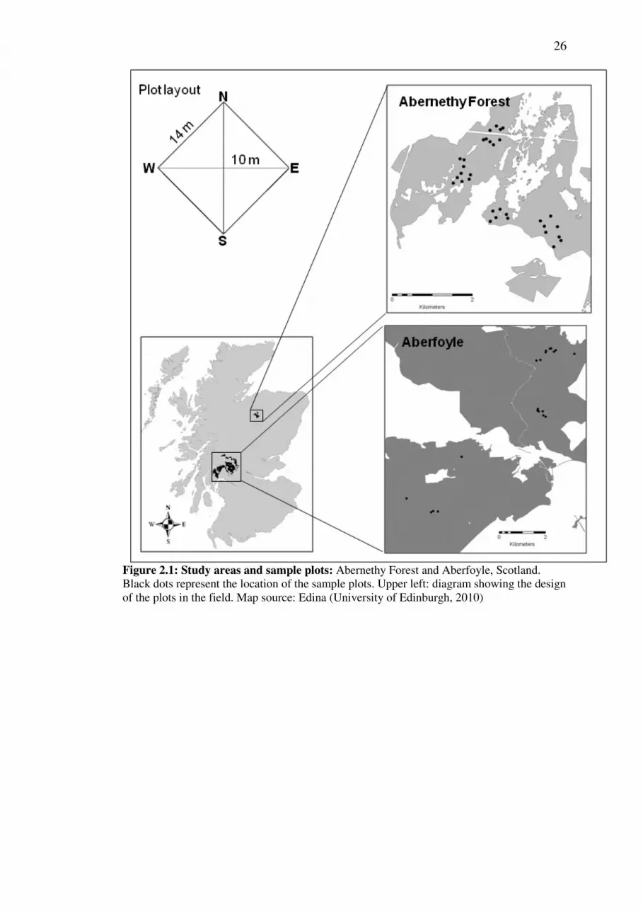
26
Figure 2.1: Study areas and sample plots: Abernethy Forest and Aberfoyle, Scotland.
Black dots represent the location of the sample plots. Upper left: diagram showing the design
of the plots in the field. Map source: Edina (University of Edinburgh, 2010)

27
2.2.2 Stands selection and sampling strategy
Sample areas at Aberfoyle and Abernethy were selected using the Forestry
Commission stockmap data as well as available digital forest data respectively
(ArcMap GIS; RSPB 2009). The stands were chosen to be representative of available
mature seed-producing habitat types for red squirrels: namely semi natural
woodlands, plantations, and a mix of both. We employed a stratified random
sampling approach. Stands were stratified by habitat type within which plots were
randomly selected. At both sites, 14 m x 14 m plots were sampled: a total of 20 in
Aberfoyle and 32 in Abernethy (Figure 2.1). Plots were pre-selected, mapped and
located on the ground using a compass and GPS (Garmin GPS map 60CSx). Within
each plot, we recorded diameter at breast height (DBH), canopy closure using a
spherical densiometer (Robert E. Lemmon Model C), and tree height using a Silva
ClinoMaster Clinometer/Heightmeter (CM-1015-2025 A). Canopy closure
measurements were made at the central point and at each of the 4 corners of the plot,
and subsequently averaged. DBH was recorded for all trees per plot. For tree height,
all trees were measured. In plots where the number of trees was greater than 30, the
height of the four trees with largest DBHs was measured and recorded.
Squirrel presence and local abundance was assessed using cone transect lines
(Gurnell et al. 2009). Our interest was in plot-level squirrel activity. We therefore
used feeding remains (cones stripped by squirrels) within each plot as an index of
micro-habitat selection by red squirrel. Grey squirrels have not yet spread to
Abernethy (Lurz & Cole, 2010, pp. 49). In Aberfoyle, although both red and grey
squirrels are present in the area, recent grey squirrel sightings have been localised
and sporadic and none were near the study sites (K. Freeman, FC Officer, pers.
comm.). Given the dense ground vegetation found in the plots and the semi-natural
arrangement of trees (absence of parallel plantation structure), a quadrat-based
approach (2 m x 2 m) was employed (Wauters et al. 2004). A total of 200 and 320
quadrats were sampled in Aberfoyle and Abernethy, respectively. This represents a
standard effort of 10 quadrats per plot. We counted both eaten and un-eaten cones.
All sampled plots contained a cone crop. This was important as the absence of food
would clearly bias the adopted approach.

28
2.2.3 Data analysis
Abernethy Forest
In an early stage of the project, a preliminary analysis was carried out considering
Abernethy Forest data only. A General Linear Model (GLM) was used to relate the
number of stripped cones (dependent variable, count data) to the stand structural
variables measured in the field, namely: total number of trees; mean tree height (m);
mean DBH (m); and mean canopy closure (%). However, the use of one study site
only does not allow for a generalisation of the results. Thus, the final analysis was
carried out considering both Abernethy and Aberfoyle data together as described in
the following section
Abernethy and Aberfoyle Forest
We used a General Linear Modelling approach and modelled the response of the
dependent variable (cones stripped by squirrel) as a combination of three
independent variables collected in the field: canopy closure, tree density and tree
height. Linear models are commonly used to explain the relationship between a
single normally distributed dependent variable Y, and one or more independent
variables (Faraway, 2005). Generalized linear models (GLM) are an extension of
linear regression commonly used to model dependent variables that are not continue
or normally distributed (Agresti, 2002).
The number of stripped cones is a count (a positive integer). Poisson regression is
usually used with count data (Zuur et al., 2007). If the variance is greater than the
mean, the data are considered over dispersed. In most real ecological applications,
this assumption is violated (Faraway, 2006). In such instance, a GLM model with a
quasi-Poisson error structure should be used. We tested our field data and found
them to be over dispersed. Therefore, we used a general linear model with a quasi-
Poisson error structure for our analysis. All analyses were carried out in the software
package ‘R’ version 2.11.1.
We also tested our data for collinearity. If the relationship between the response
variable and the covariates is not very strong (usually the case in ecological studies)
even a small amount of collinearity might affect the results of the regression (Zuur et
al., 2012, in preparation). Furthermore, the general recommendation is to have at
least 15-25 observations per covariate (Zuur et al., 2012, in preparation). The current
number of observations (i.e. 52) is on the low side for four covariates but is sufficient

29
for three. Thus, in addition to testing for collinearity, we also assessed the
relationship between the covariates and the response variable in order to decide
which variables could be disregarded (Zuur et al., 2012, in preparation).
Finally, the correlation between total cone crop per plot (i.e. whole cones plus cones
stripped by squirrels) and stripped cones was also performed in order to assess the
relationship between food abundance and habitat use by red squirrel,
2.3 Results
In Abernethy, the total number of trees per plot ranged from 3 to 74 (average 19.2 +/-
15.4 95% CI); mean DBH, from 12 cm to 79 cm (average 26.9 +/- 8.5 95% CI);
mean percentage canopy closure, from 61% to 93% (average 88.1 +/- 5.5 95% CI)
and mean tree height from 7m to 26m (average 17.6 +/- 3.1 95% CI). In Aberfoyle,
total number of trees ranged from 7 to 26 (average 16.2 +/- 7.5 95% CI); mean
percentage canopy closure from 54% to 94% (average 85.4 +/- 7.7 95% CI); mean
DBH from 16cm to 37cm (average 29.3 +/- 7.5 95% CI) and mean tree height from
15m to 24m (average 20.5 +/- 2.3 95% CI). Table 2.1 presents values for both sites,
including the total number of trees, mean DBH, mean tree height, and mean
percentage canopy closure per plot. For all these variables, we also provide averages,
standard deviations and 95% confidence interval of the mean for all plots combined.
In Table 2.1 we also present the number of stripped cones per plot. Total cone crop
ranged from 14 to 293 (average= 98.4; SD =57.7) at Abernethy and 21 to 222
(average = 83.7; SD=56.7) at Aberfoyle.

30
Table 2.1 Total cone crop, Total number of stripped cones, Total number of trees, Average DBH,
Average tree height, and % canopy closure per plot for both Abernethy Forest (Abern) and Aberfoyle
(Aberf), Scotland.
Plot number
Total cone
crop
Total number of
stripped cones
Total number
of trees
Average
DBH (cm)
Average tree
height (m)
Canopy
Closure (%)
Abern1 121 61 32 22.5 20.4 91.3
Abern2 81 4 4 26.7 15.2 61.5
Abern3 119 15 34 16.9 16.0 91.4
Abern4 119 9 22 22.9 22.4 92.0
Abern5 99 42 22 18.1 19.5 93.2
Abern6 36 4 21 23.3 23.1 93.5
Abern7 64 12 19 21.9 21.1 88.5
Abern8 108 27 15 25.8 18.8 88.0
Abern9 37 0 12 23.3 19.2 89.8
Abern10 41 4 9 12.1 6.4 73.3
Abern11 293 91 5 78.6 25.5 94.8
Abern12 100 20 12 20.2 12.0 94.2
Abern13 135 5 15 18.6 9.1 76.8
Abern14 166 14 42 15.1 8.8 77.2
Abern15 113 35 74 14.7 17.9 91.3
Abern16 25 11 23 15.4 15.9 92.2
Abern17 152 47 67 14.1 13.8 91.8
Abern18 90 17 33 17.1 14.6 88.6
Abern19 143 16 12 34.4 14.0 92.4
Abern20 88 0 7 39.5 16.2 85.2
Abern21 87 44 14 37.2 20.9 92.9
Abern22 183 18 23 23.4 15.5 91.5
Abern23 113 9 13 27.1 17.0 90.7
Abern24 58 16 7 32.3 19.2 89.0
Abern25 193 60 11 25.8 20.0 93.5
Abern26 32 3 7 28.8 15.9 91.9
Abern27 64 5 10 34.9 20.9 90.7
Abern28 57 5 11 30.8 21.6 90.4
Abern29 14 2 3 41.5 20.4 69.9
Abern30 62 32 11 33.0 18.3 92.6
Abern31 85 55 15 31.5 24.5 91.4
Abern32 72 3 11 34.0 19.1 89.2
Aberf33 35 18 14 35.3 23.0 87.6
Aberf34 21 0 13 27.0 16.1 54.4
Aberf35 80 11 7 35.1 22.3 93.1
Aberf36 76 0 22 22.9 15.6 90.2
Aberf37 49 6 18 32.5 21.0 93.6
Aberf38 41 4 18 27.4 19.2 93.1
Aberf39 222 0 9 35.2 24.1 84.4
Aberf40 93 48 11 37.3 22.7 86.5
Aberf41 139 7 16 26.2 21.3 91.1
Aberf42 88 2 11 35.1 21.7 80.7
Aberf43 183 3 12 35.3 21.5 83.3
Aberf44 68 2 8 34.7 21.9 77.3
Aberf45 118 21 9 32.6 21.7 80.0
Aberf46 57 22 9 32.2 23.3 88.0
Aberf47 176 4 12 35.5 22.8 81.1
Aberf48 27 1 28 21.7 18.5 93.8
Aberf49 38 3 30 18.6 16.2 84.8
Aberf50 38 25 30 18.4 19.5 87.2
Aberf51 78 57 36 16.8 17.1 89.6
Aberf52 46 12 11 26.0 21.4 87.8
Mean 92.8 17.9 18.1 27.8 18.7 87.1
SD 57.2 20.4 13.9 10.5 4.1 8.2
95% CI
31.9
(76.8-108.7)
11.1
(12.4, 23.5)
7.5
(14.3, 21.8)
5.8
(24.9, 30.7)
2.2
(17.6, 19.8)
4.5
(84.8, 89.3)

31
Abernethy Forest
We checked the data for collinearity and we found that mean tree height and mean
DBH were significantly correlated (rs= 0.55, n=32, p � 0.001). Correlations between
mean tree height/mean DBH and the number of stripped cones were also assessed
and found to be very similar (rs = 0.37 and 0.38; p < 0.04 and 0.03 respectively, n
=32). Between tree height and DBH, only the latter was used in the General Lineal
Model (GLM) analysis.
The results of the GLM analysis indicate that mean DBH, mean canopy cover and
total number of trees per plot were significant predictors of the number of cones
stripped by squirrels (p < 0.006, 0.01 and 0.03 respectively). DBH is the independent
variable which contributes the most (coefficient = 2.6) followed by canopy cover and
number of trees (coefficients = 0.09 and 0.02 respectively). The resulting model
(presented below) explains 46% (R 2 = 0.46) of the variation in the field measured
data.
SC = -6.6 + (2.6) DBH + (0.09) CC + (0.02) NT
Where SC is the total number of stripped cones, DBH is mean diameter at breast
height, CC is mean canopy closure and NT is total number of trees.
Abernethy and Aberfoyle
Combining the data from the two sites, we tested the relationship between the
number of stripped cones -as an indicator of squirrel habitat use- and the different
stand structure variables.
The data was checked for collinearity and it was found that mean DBH was
significantly correlated with the number of trees (rs= -0.58, n=52, p � 0.001) and
with mean tree height (rs = 0.59, n=52, p � 0.001). We assessed the relationship
between these three covariates and the response variable in order to decide which
variables not to use for the model. Mean DBH did not show a stronger correlation
with the number of stripped cones (rs= 0.23, n=52, p � 0.009) than the number of
trees (rs= 0.25, n=52, p � 0.008) or tree height (rs= 0.21, n=52, p � 0.014). Therefore,
DBH was not used in the GLM analysis. No other correlations were observed among
the variables.

32
With respects to food abundance, correlation between total cone crop and number of
stripped cones was low to moderate (rs=0.37, n=52, p<0.007).
The results of the GLM analysis indicate that forest structural variables measured in
the field were significant predictors of the number of cones stripped by squirrels
(Table 2.2).
Mean canopy closure and total number of trees per plot are the variables which
contribute the most to the incidence of cones stripped by squirrels (p � 0.01 and 0.03
respectively; Table 2.2). Squirrels are known to prefer seeds with high nutrient
content (Gurnell 1987), and nutrient content in Scots pine has been found to increase
with tree height (Grönwall 1982). Thus, mean tree height was considered to be an
important biological predictor of red squirrel tree selection and was retained (p �
0.058).
Table 2.2: Results for the GLM model (with a quasi-Poisson error structure) relating number
of stripped cones to forest structure parameters
Regression
parameters
Slope
coefficient
Standard
Error
t value p value
�
Constant -6.503725 2.935908 -2.215 0.0315*
Mean canopy
closure
0.083300 0.032195 2.587 0.0128*
Number of trees 0.017996 0.008096 2.223 0.0310*
Mean tree height 0.083209 0.043005 1.935 0.0589**
Significance code (alpha level): * 0.05 - **0.1
The resulting GLM is presented below, where SC is the total number of stripped
cones, CC is mean canopy closure, NT is total number of trees and TH is mean tree
height.
SC = -6.5 + (0.083) CC + (0.018) NT + (0.083) TH

33
The model explains 43% (R 2 = 0.43) of the variation in the field measured data.
Figure 2.2 shows the scatter plot of observed vs. predicted number of cones stripped
by red squirrels.
Figure 2.2: Scatter plot. Observed versus Predicted values of number of Scots pine cones
stripped by squirrels using the GLM : Y = µ + �c + �d + �h + � , where Y is the dependent
variable and �c, �d, �h are covariates describing Canopy Closure, Tree Density and Tree
Height respectively. The Residual Error is described by �. Line of unity (1:1) is shown in
blue.
34
2.4 Discussion
Our results show that forest structural characteristics are significant predictors of the
number of cones stripped by squirrels and therefore suggest that canopy closure, tree
density (and potentially tree height) are important factors in influencing foraging
behaviour of red squirrels. This has implications for conservation management. The
current strategy for red squirrel conservation with respect to forest management is
based on the selection of a set of suitable strongholds sites (see for example
http://www.forestry.gov.uk/forestry/infd-7q3ft8), where viable red squirrel
populations can be sustained over the long term (Parrott et al., 2009). Management
recommendations currently focus on overall woodland size (e.g. > 2000 ha), tree
species composition and age structure to provide a dependable seed food supply,
guidance on forest operations such as thinning and felling to reduce detrimental
impacts on local populations, monitoring to detect population trends and changes in
distribution of both grey and red squirrel, grey squirrel control to prevent or reduce
the risk of disease spread and reducing the potential for grey squirrel competition by
excluding large-seeded broadleaves in and around stronghold areas (Gurnell &
Pepper 1993, Gurnell et al. 2009, Lurz et al. 1998, Pepper & Patterson 1998,
Bruemmer et al. 2010).
Our findings extend these recommendations by stressing the need to consider forest
structure at the sub-stand level when implementing conservation measures. More
specifically, our findings highlight and for the first time quantify the importance of
mean canopy closure and total number of trees per plot as key structural variables.
This suggests a preference of red squirrels for denser stands which concords with
previous research carried out in the UK, where red squirrels were observed to avoid
thinned, open stands of trees (Gurnell et al. 2002). Studies conducted elsewhere on
arboreal squirrels’ habitat preferences also reach comparable conclusions: Smith et.
al. (1994) found that Mount Graham red squirrel (Tamiasciurus hudsonicus
grahamensis) midden sites (i.e. sites were cones are stored for winter food supply)
were located in areas of high tree densities and high canopy closure (> 70%) in
Piñaleno Mountains, Arizona. Moreover, Nelson et al. (2005) highlighted the
importance of closed canopies for the Delmarva fox squirrel (Sciurus niger cinereus
L), while McKinney and Fiedler (2010) found that basal area, canopy closure and

35
canopy height were significant predictors of the distribution of arboreal squirrels in
the Rocky Mountains (USA). Besides, a habitat suitability index model developed by
the Fish and Wildlife Service, Department of the Interior (U.S.A, 1987) to predict
grey squirrel habitat, regarded canopy closure and tree density as variables directly
related to the provision of cover for squirrels. It is important to note however, that
these preferences are not generic to squirrels, but species specific. Whilst our results
allow an assessment of habitat suitability for red squirrels in Scots pine habitats,
there is a need to improve our understanding of these preferences in other habitat
types and their underlying causes. Canopy cover and tree density may be linked to
optimal foraging by allowing speedy movement through tree crowns without a need
to descend to the forest floor; and reflect a need for cover to reduce predation risks.
Tree height was marginally significant in our GLM model (p � 0.058), but may be an
important predictor of seed quality. Grönwall (1982) studying habitat selection in red
squirrels in Sweden found a significant correlation between tree height (and age) and
seed nutrient content (e.g. crude protein, phosphorus, magnesium).
Our findings suggest that not all structural characteristics are equally important for
habitat selection, and indicate a ‘hierarchy’ for red squirrel habitat selection. In Table
2.3 we present a basis for building such hierarchical framework for red squirrel
habitat selection in the UK. We start from the premise that decision-making is a
result of processes involving a succession of choices, themselves influenced by
preferences. Hierarchically, food availability and quality are the most important
factors influencing habitat choice and determining red squirrel habitat use. If food is
available, our results show that stand structure is then a critical second factor in
determining where squirrels forage.

36
Table 2.3: Habitat design for red squirrel conservation In a hierarchy of decision, food
availability is the most important component determining red squirrel abundance and habitat
use. Our results show that when food is available, stand structure is a critical factor in
determining red squirrel habitat use
Habitat suitability Forest management
option
Reference Currently
accounted for in
management?
Habitat type
Conifer species
diversity
Gurnell 1983 &
1987; Lurz et al.
2000; Poulsom et al.
2005
YES
Seed availability &
quality
Suitable age
structure
Gurnell 1983 &
1987; Lurz et al.
2000; Poulsom, et
al. 2005
YES
Fringe planting Pepper & Paterson,
2001
YES
Stand structure
- Closed canopy
- High tree density
- Tall trees
This study
NO
Our results indicate that open forests (or late stage thinned) may be of limited
suitability for red squirrels. This has significant implications for further developing
the UK strategy for red squirrel conservation as well as for improving the
management of woodlands to support red squirrel populations. Current forest design
for red squirrels contemplates diversification of conifer species and age class to
ensure continuous food supply and the avoidance of large-seeded broadleaved
species, such as oak (Quercus petraea), chestnut (Castanea), beech (Fagus) and
hazel (Corylus). This paper highlights the importance of considering as well the
structural characteristics of forest stands and the need to provide dense stands and
maintain a contiguous canopy cover in parts of the forest. For management, these
results identify the need for methods to extract and utilise structural data (notably
canopy closure and total number of trees) to derive habitat suitability information
over large forest areas. These are needed to assess current suitability of strongholds
and to plan conservation management actions for red squirrels and other endangered
forest dwelling species. One potential future research avenue would be to link field
data on habitat selection with forest structural data extracted using remote-sensing
approaches (e.g. LIDAR, Patenaude et al., 2004).

37
CHAPTER 3
LiDAR data processing for red squirrels habitat mapping
____________________________________________________________________
The importance of forest structural parameters for red squirrels habitat mapping was
addressed in the previous Chapter: Canopy closure, number of trees and tree height
were found to be significant predictors and to explain 43% of the variation in cones
stripped by squirrels. However, the analysis is restricted to a few sample plots due to
a limited availability of structural data along with cost-efficient data collection
methods. The use of remote sensing -in particular Light Detection and Ranging
(LiDAR) - enables cost efficient forest structure assessment at large scales.
This chapter provides a brief introduction to LiDAR remote sensing as well as
detailed description of methodologies used to retrieve the three parameters that relate
to habitat suitability for red squirrels: mean canopy cover, mean tree height and total
number of trees. Accuracy assessment is performed by comparing LiDAR retrieved
structural parameters to field measurements at the plot level, and results are
presented and discussed. The relationship between field measured canopy closure
and LiDAR estimated canopy cover is also discussed.
__________________________________________________________
3.1 Introduction
3.1.1 LiDAR remote sensing
LiDAR (Light Detection and Ranging) is an active remote sensing technology that
uses the time that a laser beam takes to travel to and from a target to calculate
distances. Laser pulses descend to the ground and form a circular footprint where the
pulse hits the ground. These pulses are reflected by objects on the ground or by the
ground itself and the distance between these targets and the sensor is calculated by
multiplying the return time (i.e. time elapsed between the laser beam leaves the
sensor, hits a target and returns to the sensor) by the speed of light and divided by
two (Mather, 2004). Detailed technical description of LiDAR can be found in
Baltsavias (1999). The main characteristic and advantage of LiDAR remote sensing
in forestry is that it allows for direct retrieval of canopy height (Brovelli et al., 2002).

38
LiDAR sensors can be categorised as discrete return or full-waveform. The main
difference between these two systems is how they sample three-dimensional
structure. Full-waveform systems record reflected energy over equal time intervals,
and the level of detail in a laser footprint is given by the number of recording
intervals. On the other hand, discrete systems record either one (single-return
systems) or a small number (multiple-return systems) of returns for each pulse sent to
the ground from the aircraft (Lim et al, 2003). Both LiDAR systems consist of a
combination of three pieces of equipment which are mounted on an aircraft: laser
emitter-receiver, Global Positioning System (GPS) and Inertial Navigation System
(INS) (Brovelli et al., 2002).
The utility of each system depends on the size of the footprint. For most discrete
return systems, footprints are in the order of 0.2 to 0.9 m, while for full waveform
systems, footprint size ranges from 8 to 70 m (Lim et al, 2003). Therefore, if used for
forest applications, full waveform LiDAR system will be more likely to provide
information on a forest area including multiple elements while discrete return will be
capable of characterizing individual trees (Lim et al, 2003). In this project, only data
acquired by discrete return LiDAR system were used as it provides the spatial
resolution needed.
3.1.2 LiDAR data processing for red squirrel habitat mapping
LiDAR data consists of a collection of points where the x, y and z coordinates of the
points are known. This cloud of points consists of terrain -or bare Earth - and off-
terrain (i.e. objects on the surface) points. The first step in LiDAR data processing is
usually generating a digital terrain model (DTM) which involves the filtering of
returns in order to identify those that correspond to the ground (bare Earth points)
(Brovelli et al., 2002). The general approach to generate a DTM from LiDAR data
consists on taking the lowest value within a grid cell, where the size of the cell will
depend on the spatial resolution of the data (i.e. pulses/m2). The missing values are
then estimated by interpolation (Maltamo et al., 2004). The approach to generate a
digital surface model (DSM) from LiDAR data is similar to the described above: in
this case, the highest value within each grid cell is detected and the missing values
are calculated by interpolation (Maltamo et al., 2004). Finally, canopy height model
(CHM) is calculated by subtracting the digital terrain model from the digital surface
model. It is beyond the scope of this Chapter to critically review the several filtering

39
techniques to discriminate between ground and above ground points and algorithms
that exist to generate digital terrain and canopy height models. More detailed
summaries can be found in Kraus & Pfeifer (1998); Brovelli et al (2002), Reutebuch
et al, (2003); Meng et al (2010) and Sulaiman et al. (2010). Furthermore, detailed
reviews of the use of LiDAR for forest applications can be found in Lim et al (2003),
Næsset et. al, (2004), Hyyppä et al (2008).
This chapter will focus on the use of LiDAR data to retrieve forest structural
parameters that relate to red squirrel habitat suitability at the plot level, namely mean
canopy cover; mean tree height and total number of trees (see Chapter 2). Several
researchers have explored different approaches to generate these products using
LiDAR data. A review of previous studies is presented in the following sections;
while a summary of the use of LiDAR for habitat assessment is provided in Chapter
4.
3.1.2.1 Canopy cover
The most common approach used to estimate canopy cover from LiDAR data
consists of calculating the proportion of returns that hit the canopy, where canopy is
defined as vegetation above a specific height threshold (Korhonen et al., 2011). This
is analogous to the method used by ecologists to estimate ground vegetation cover,
which consists of dividing the number of points covered by vegetation by the total
number of sampled points within a reference frame (i.e. quadrat; Jennings et al.,
1999).
In the case of LiDAR remote sensing, the approach involves dividing the canopy
portion of the returns by the total of the returns (i.e. canopy returns + ground
returns). Usually only first returns are considered as last and intermediate returns
provide little useful information. The height at which field measurements of canopy
cover are taken (i.e. breast height) can be used as threshold to discriminate canopy
from non-canopy (Korhonen et al., 2011).
This approach has been used by several researchers. Hyde et al., (2005) estimated
canopy cover using waveform LiDAR for a mixed-conifer woodland in Sierra
National Forest, California. They separated the ground and canopy portions of the
waveform and calculated canopy cover by dividing the canopy portion of the
waveform by the total energy in the waveform. In their study, Hyde et. al. (2005)
also used optical data: they classified the Quickbird Near-Infrared (NIR) band into

40
forest and non-forest (based on visual observation); then the ratio between the two
classes was computed, and the result (i.e. 1.6) was used to assist in the discrimination
between canopy and non-canopy in the image resulting from the ratio between the
canopy portion/total energy in the waveform. In this study, the accuracy of canopy
cover estimated from LiDAR was evaluated by assessing the correlation between
field measured and LiDAR derived canopy cover which showed an agreement of
81% (0.81, root mean square error (RMSE) =9.4%, n =40, P<0.00). Canopy cover
was measured in the field using a Moosehorn densiometer.
LiDAR canopy cover has also been used in studies without direct field validation.
For instance, Stephens et. al (2012) used canopy cover derived from LiDAR along
with other LiDAR metrics in a linear regression to predict carbon content at the plot
level in 246 plots randomly distributed in forests throughout New Zealand for which
both LiDAR and field inventory data were available. Results showed that LiDAR
canopy cover and 30th
percentile of height explained 74% of the variation in carbon
content (R2 =0.74, n=246, P<0.05).
The disadvantage of using the proportion of laser beams that hit the canopy to
estimate canopy cover is that large LiDAR scan angles can produce slightly biased
canopy cover estimates (Korhonen et al., 2011). However, previous research on this
issue has shown that at the scan angles LiDAR data is usually acquired (not larger
that 18°), bias does not represent a problem. For instance, Morsdorf et al. (2008)
carried out a study to assess the effects of LiDAR scan angles on biophysical forest
parameters derived from LiDAR data. In their study, they only used LiDAR data that
had been acquired with a scan angle of +/- 7.5, and their results showed that -at those
small scan angles- the effects on canopy cover estimates are negligible. Furthermore,
Richardson et al., (2009) and Ahokas et.al., (2005) tested the effects of larger scan
angles on forest products derived from LiDAR. They found that scan angles up to
10° and 15° respectively had no or very little influence on canopy cover estimates.
3.1.2.2 Individual tree delineation
In order to estimate the number of trees in a given area it is necessary to detect
individual trees first. Several algorithms have been developed to delineate individual
trees using LiDAR data (Vauhkonen et al., 2012).
The watershed technique is one of the approaches that have been widely used to
delineate individual trees. This approach is based on detecting

41
the edges (valleys) of each crown in the canopy model, and the top (peak) of
individual trees (Doo-Ahn Kwak et al., 2007).
Gougeon’s (1995) algorithm, based on the watershed technique, works by detecting
the lowest pixels (or local minima) in a given n x n window, and then it follows the
“valley pixels” -or pixel with values that are lower than their neighbours- until it
delimitates a crown. A threshold, to allow for the detection of the local minima, is
required to be defined by the user. This threshold or reference value represents the
average height of the lower part of the crowns for a given study area and can be
estimated from a histogram as shown in Figure 3.1 (Rahman & Gorte, 2009) or from
empirical data. García et al. (2007) applied this algorithm to a sitka spruce plantation
in Scotland and found that it delineated individual trees with an accuracy of 77.9 %,
where the trheshold was estimated by averaging the height of the lowest part of the
tree crowns measured in the field (García et al., 2007).
Figure 3.1: LiDAR data histogram (height (m) Vs frequency) showing how the height of the lowest
part of the crowns (reference height) can be estimated (Rahman & Gorte, 2009)
However, most algorithms are based on the local maxima approach, which consists
in finding the pixel with the highest value within a n x n window or kernel (Popescu
et al., 2003; Vauhkonen et al.,2012) The local maxima technique is based on the
assumption that those local maxima or pixels with highest values represent the top of
a tree crown (Popescu et al., 2003). Most of these algorithms use the canopy height
model as the input file (Rahman & Gorte, 2009).
Popescu et. al. (2003) developed an algorithm which applies the local maxima
technique using a variable-size window. This method requires maximum and
minimum crown diameters and allometric relationships between tree height and
crown diameter which are used to determine the appropriate window size. To finally
delineate the tree crown, a fourth-degree polynomial function is used, allowing for

42
the modelled crown to have a concave shape. When applied to a sitka spruce
plantation in Scotland, this algorithm delineated trees with an accuracy of 89.3%
(García et al., 2007).
A local maxima technique has also been combined with segmentation to delineate
trees in boreal forests. Hyyppa et al., (2001) developed an algorithm which combined
local maxima and segmentation to delineate individual trees. The algorithm works by
applying a filter to the canopy height model first to suppress noise. Then a local
maximum (or seed point) is detected, and from there the crown is delineated by
incorporating pixels using a seeded region growing method1. The crown is
considered to be delineated when a minimum threshold, defined by the user, is
reached. This algorithm was applied to a study carried out in a semi-natural boreal
forest in Finland by Maltamo et al. (2004). Tree species present in the forest were
Norway spruce (Picea abies L.), Scots pine (Pinus sylvestris) and silver birch (Betula
pendula Roth.). In this study, out of 682 trees, 265 were correctly identified
(approximately 39%) using LiDAR. When only dominant trees (i.e. trees or shrubs
with crowns receiving full light from above) are considered, the accuracy increased
to 83% (i.e. 245 out of 295 dominant trees).
Lee et al (2010) used a similar approach (i.e. local maxima plus segmentation) to
detect trees in two managed forests composed of the same pine species (loblolly
pine, Pinus taeda L.) in North-Central Florida, USA. Individual trees were detected
with an overall accuracy of 95.1%.
The question of which algorithms produce more accurate results has also been
addressed: In a recent study, Vauhkonen et al. (2012) compared the accuracy of a
number of tree-detection algorithms under different types of forests. They applied six
tree-detection different techniques to both conifer and deciduous forests in Brazil
(deciduous: Eucalyptus), Germany (conifers: Scots pine and deciduous: oaks
Quercus rubra, European beech Fagus sylvatica and silver birch Betula pendula),
Norway (conifers: Scots pine and Norway spruce) and Sweden (conifers: Scots pine
and Norway spruce). Airborne data point density (i.e. pulses/m2) were 1.5 (Brazil), 7
(Norway), 30 (Sweden), 7 and 16 (Germany). An in depth description of each
1 Seeded region growing method can be summarised in 3 steps: 1) Choose the seed pixel or local
maxima; 2) Check the neighbouring pixels and add them to the region if they meet the criteria (usually
a threshold is used); 3) repeat step 2 until no more pixels can be added to the region (Jain et. al.,
1999).

43
algorithm can be found in Vauhkonen et al., (2012). Summing up, the algorithms
worked as a combination of: local maxima and crown segmentation based on point
clustering (algorithm #1); voxel2 space and morphological algorithm (i.e. crown
boundaries detection, algorithm # 2); segmentation based on tree spacing (algorithm
# 3); local maxima adjusted by residual tree height (algorithm #4); segmentation
based on tree crown models (algorithm # 5) and adaptive filtering based on CHM
height values (algorithm # 6). Algorithms 1 and 2 used point data while the others
used the CHM (i.e. raster file). In general, the different algorithms performed
similarly under the different forest conditions. It is beyond the scope of this thesis to
provide the exact tree detection rates of each algorithm for each study area and for
each point density. Instead, the main findings are summarised as follow: a) the
general success of tree detection was strongly linked to the tree density and spatial
distribution of trees; b) an increase in laser data point-density improved the
performance of tree detection algorithms, in particular for the point-based ones; and
c) all algorithms performed better in conifer forests.
Local maxima algorithms have also been found to fail to identify small trees
surrounded by bigger and higher ones (i.e. suppressed trees) and individual trees in
deciduous woodlands where the crowns of the trees are not clearly separated from
one another, and when there is considerable overlapping between crowns (i.e. very
young conifer plantations) (Hyyppa et al., 2001). However, these limitations are not
exclusive to the local maxima approach. In their comparison of six different
algorithms, Vauhkonen et al., (2012) found that while all algorithms successfully
detected the same dominant trees, they failed to detect most of the suppressed trees.
This seems to reinforce the concept that tree detection is likely to be more dependent
on tree density and spatial distribution than on the algorithm itself.
3.1.2.3 Mean tree height
LiDAR remote sensing has been widely used to estimate canopy height. Several
authors have explored different approaches to retrieve individual tree height from
LiDAR data and have assessed the accuracy of those estimations. Results suggest
that LiDAR derived canopy height tends to underestimate height, due to two main
reasons: laser pulses missing the top of the trees and ground height overestimation
2 Voxel: Volumetric Pixel or Volumetric Picture Element
44
(low number of pulses reaching the ground). For detailed reviews on LiDAR derived
tree height see Suarez et al (2005); Maltamo et al (2004), Koukoulas et al (2005).
This section will focus on the estimation of mean canopy height at the plot level as
this is the parameter which relates to habitat preferences by red squirrels (see Chapter
2). Previous studies have shown that using arithmetic mean of laser heights leads to
underestimation of field mean tree height, in particular in those plots where large
gaps exist (i.e. low number of trees) and that upper percentile heights correlate well
with field plot-level mean and top tree height (Naesset, 1997; Lefsky, 2010;
Patenaude, 2004). In particular, 90th
percentile which has been found to correlate
well with mean tree height, and 99th
percentile, often used for top tree height (Rosette
et al, 2009; Hopkinson et. al. 2008).
The correlation between LiDAR percentiles and field tree height has been explored
by a number of researchers. For instance, Popescu et al (2002) used linear regression
to relate LiDAR estimated with field measured parameters in a mixed deciduous –
conifer forest in Virginia, US. They found that 90th
percentile was a significant
predictor of mean tree height (P< 0.05) and explained 35% of the variation in field
data (R2 = 0.35; n=24).
Hopkinson et al (2008) performed Pearson correlation between LiDAR metrics and
field measurements in a forest of heterogeneous species composition, 50km north of
Toronto, Canada. Results showed strong correlation between LiDAR 90th
percentile
and field mean tree height (r = 0.63, P< 0.01, n=19). However, 90th
percentile is not
the only LiDAR metric that has been successfully associated with mean tree height:
Correlation between LiDAR 95th
percentile and field mean height was also assessed
by Hopkinson et al (2008) and found to be also strong (r = 0.59, P< 0.01, n=19).
Furthermore, Holmgrem et al. (2004) carried out a study in a forest in Norway,
mainly composed of Norway spruce and Scots pine. They found a high correlation
(r=0.995, n=29, P< 0.00) between laser-predicted and field-measured mean tree
height, where laser mean height was predicted using 95th
percentile.
In this Chapter, both 90th
and 95th
percentiles of LiDAR canopy height will be
compared to mean field tree height at both Abernethy and Aberfoyle forests to assess
which of these metrics better represent mean tree height at the plot level.

45
3.1.3 FUSION
FUSION (Version 2.90) was developed by the United States Department of
Agriculture and it is distributed free of charge.
This package was developed to visualize, analyse and process LiDAR data. FUSION
allows users to display, import/export LiDAR data in different formats, and to create
products such as digital terrain models, digital surface models, canopy height models
and canopy cover.
The accuracy of products generated using FUSION has been tested by a number of
researchers. For instance, Reutebuch et. al. (2003) compared digital terrain model
derived from LiDAR to 347 checkpoints elevation measured in the field.
Checkpoints were located in different areas of a conifer forest in a mountainous area,
ranging from clear cut to dense vegetation. Their results showed that elevation values
obtained from LiDAR were highly accurate. Differences between LiDAR DTM and
elevation measured in the field ranged from –0.63 to 1.31 m and the mean of the
difference was 0.22 ± 0.24 m (mean ± SD).
FUSION allows for individual trees to be manually identified and measured. In a
study carried out by McGaughey et al. (2004), a total of 112 trees were measured in
the field, manually identified in a LiDAR canopy height model and measured within
FUSION and their heights were compared. Mean height difference was -0.29 m and
SD = 2.23.
FUSION based tree heights were also compared to those generated using other
packages (TIN, ArcGIS) by Gaulton (2008). Both canopy height models were
compared and found to be very similar, with a largest difference of 1 m in maximum
tree height (34.50 m for FUSION; 35.52 for TIN). In this study, FUSION based tree
heights were closer to the height measured in the field (mean difference = -0.06m
and -1.08m and RMSE = 1.43m and 1.91m for FUSION and TIN respectively,
n=49). FUSION has been widely used and more exhaustive descriptions of its
application than are possible here can be found in the FUSION website
(http://forsys.cfr.washington.edu/JFSP06/index.htm). The main advantage of
FUSION is that it allows for operational processing of large amounts of LiDAR data
at no cost. However, critical reviews of FUSION advantages and limitations
remained yet to be published at the time this thesis was written.

46
3.2 Methodology
3.2.1 LiDAR data processing
LiDAR data at Abernethy Forest and Aberfoyle Forest were acquired and delivered
by different providers and in different format files, as follow:
Abernethy Forest
LiDAR data at Abernethy Forest was collected by the NERC Airborne Research
Facility (ARSF). Data provided consisted of eight (8) text files, one for each LiDAR
flight-line. Before being delivered to the final user, LiDAR data quality is tested for
noise and points are classified with the number 1 or 7, where points classified with
the number 7 are suspected to be “noise” or returns outside the range of realistic
elevations (i.e. caused by atmospheric aerosols, birds, or low-flying aircraft). These
points are not removed by the provider but a program is delivered with the data
which creates new text files where the noise has been removed.
Aberfoyle Forest
LiDAR data for Aberfoyle Forest was provided by Infoterra. Data was delivered as a
number of XYZ files (tiles in ASCII format). Noise had already been removed. The
program XYZConvert (FUSION) was used to convert XYZ files into a format that
could be processed within FUSION.
LiDAR data characteristics are summarised in Table 3.1
Table 3.1: Characteristics of the LiDAR data for both Abernethy and Aberfoyle, Scotland
Abernethy Aberfoyle
Date 27th November 2009 8
th May 2008
Resolution (pulses / m2)
2 pulses / m2 1 pulses / m
2
Data provided First, second, and last return- intensity
First and last return
Scan angle +/- 18° +/- 20°
Average flight altitude 1760 m 1310 m
Both LiDAR datasets (i.e. Abernethy and Aberfoyle) were mapped to a geographic
co-ordinate system (British National Grid) using on-board attitude and positional
information with additional ground control points. Data was compared to Ordnance

47
Survey Maps and judged to be accurately positioned and no further corrections were
applied.
3.2.2 DTM and CHM
Once LiDAR data from both Abernethy and Aberfoyle Forests had been converted
into a format that could be processed within FUSION, the following step is to
generate a digital terrain model (DTM) by filtering those returns that are more likely
to correspond to bare Earth. The software used to generate the DTM was FUSION
(Version 2.90). Creating a DTM within FUSION requires the use of two programs.
First, GroundFilter creates a surface where only returns that correspond to bare earth
are kept. The algorithm used, which is described in detail in Kraus and Pfeifer
(1998), is based on linear prediction and works iteratively. First, an average surface
(i.e. a surface between top of the vegetation and ground) is created from all input
points. On a second stage, weights are computed for each point, according to the
distance from the average surface and direction (given by the positive or negative
sign of the residuals). On a final stage, and given a threshold g, points with residuals
smaller than g are given a weight of 1, and points with residuals larger than g are
given a weight of 0. In the final iteration, those points -that were given a weight of 1-
whose distance from the average surface is less than a user-specified tolerance are
classified as bare earth points.
The number of iterations was set to 30, the tolerance was set to 0.1m (default value)
and the rest of the parameters were also defined according to recommended defaults
(McGaughey, 2009).
In the second part of the process, the program GridSurfaceCreate is used to finally
create the DTM. This program uses the file created by GroundFilter and interpolates
the values identified as bare earth. GridSurfaceCreate computes the elevation of each
grid cell using the average elevation of all points within the cell. The option to
smooth the data is given but it is not recomemended for vegetated areas since it can
result in loss of surface detail (McGaughey, 2009). Based on LiDAR data spatial
resolution (i.e. 2 pulses/m2 at Abernethy and 1 pulse/m
2 at Aberfoyle) cell size was
set to 1 m for both forests. The resulting files were exported as ASCII files and
imported into ArcGIS (V 9.0) to create raster files.

48
FUSION was also used to create a canopy height model. The program CanopyModel
creates a canopy height model (CHM) by assigning the elevation of the highest
return within each grid cell, where the size of the cell is given by the user. The
algorithm uses both the file which contains all the returns and the DTM (bare earth
surface) to subtract the ground elevations and generate a CHM (McGaughey, 2009).
Cell size was again set to 1m, and the files created in FUSION were also exported as
ASCII files and imported into ArcGIS to create raster files.
Table 3.2 presents a summary of the tools and programs used and files created in
every stage of the LiDAR data pre-processing.
Table 3.2: Summary of LiDAR data pre-processing described in this section
Process Program Output file
“Noise” filtering (only for Abernethy Forest data)
pt_cloud_filter (NERC- ARSF)
Text file free from noise
Format conversion (only for Aberfoyle data)
XYZConvert (FUSION
FUSION format file - first and last returns
Bare earth points filtering GroundFilter (FUSION)
FUSION format file with only points identified as bare earth
DTM creation GridSurfaceCreate (FUSION)
Digital terrain model
Canopy Height Model creation
CanopyModel (FUSION)
Canopy height model
ASCII files creation FUSION DTM and CHM ASCII files
Raster files creation ArcGIS DTM and CHM raster files
DTM validation
As part of this study, elevation measurements in the field were not required. Albeit
the fact that the equipment required was not available at the time that the field work
was being conducted, absolute accuracy of digital terrain model (i.e. elevation above
the sea level) is not of interest for this project: the main aim is to assess whether
spatial changes in elevation are well represented, as these would influence canopy
height. For this purpose, the fact that several studies have already provided evidence
that LiDAR produces accurate digital terrain models under dense forest canopy (for
example, Kraus & Pfeifer; 1998; Reutebuch et al, 2003) is considered sufficient.
Nevertheless, an assessment of the consistency of LiDAR retrieved DTM was
conducted by comparing results with the Ordnance Survey (OS) DTM. The purpose

49
of this evaluation is to assess whether gross systematic errors can be detected and, if
possible, whether this error can be attributed to LiDAR or OS DTM. This evaluation
was conducted for both Abernethy Forest and Aberfoyle Forest.
Ordnance Survey (OS) DTMs are created using the height information contained in
contour files. These contours were surveyed by photogrammetry – stereo
interpretation of aerial photography – in an initial capture programme which was
completed in 1987. The results achieved depend on the density of height data
contained in each contour file. OS DTMs are provided with 1 m height resolution
and 10 m horizontal grid interval. The general height accuracy is +/- 2.5m to 5m;
although in mountain and moorland areas the accuracy can be lower. In some flat
areas where there is little height information, contours and spot heights may be a
great distance apart, this can cause irregularities in the DTM which appear as slight
terracing of the terrain (Ordnance Survey, 2001).
The comparison between the LiDAR and OS DTMs was performed as follow:
- A map of the difference between LiDAR and OS DTMs was created within
ArcGIS and differences were classified into 3 intervals: -5 to -2.5, -2.5 to 2.5m and
2.5 to 5 (Figure 3.4). These thresholds were based on the OS DTM accuracy range
(+/- 2.5m to +/- 5m).
- Ground elevation retrieved from LiDAR data was compared to the OS DTM at the
plot level. Both DTM values (LiDAR and OS) were extracted for the plots’ central
points (i.e. 32 in Abernethy and 52 in Aberfoyle) and the correlation between the two
sets of values was explored.
- The mean difference between LiDAR and OS DTM was statistically tested to
assess the presence of systematic error.
3.2.3 Canopy Cover
Canopy cover was estimated as the proportion of laser beams that hits the canopy,
where canopy is defined as vegetation above a specific height threshold (Korhonen et
al., 2011). The programme Cover (FUSION) was used to calculate canopy cover by
dividing the number of first returns above a given height threshold (height-break) by
the total number of returns over a specific area (cell size). Height break was set at
1.3m (following literature recommendations; Korhonen et al., 2011); cell size must

50
be large enough (i.e. larger than individual tree crowns) in order to provide a
reasonable sample area to assess vegetation cover. For most forest types, cell sizes of
5m to 15m produce good results (McGaughey, 2009). To allow for comparison
between LiDAR derived canopy cover and field measured canopy closure, the cell-
size used was the size of the field plots (i.e.14 m). Output file values range from 0 to
100 percent.
Canopy closure was measured in the field using a concave spherical densiometer
(Robert E. Lemmon Model C). Measurements were made at each of the 4 corners
and at the central point of the plot and subsequently averaged.
Although canopy cover and canopy closure have been frequently used as
synonymous, it is important to remark here that there is a clear difference between
these two ways of quantifying forest canopies: While canopy closure represents the
proportion of the sky hemisphere obscured by vegetation when viewed from a single
point (Jennings et al., 1999), canopy cover reflects the proportion of the forest floor
covered by the vertical projection of the tree crowns (ibid). In other words, canopy
cover is a vertical measure of gaps between crowns; while canopy closure includes
all gaps in the field of view (Figure 3.2).
Figure 3.2: a) canopy closure, b) canopy cover (Jennings et. al., 1999)
Canopy closure –and not canopy cover- was measured in the field for this project as
this is the variable most traditionally associated with ecological applications such as
habitat assessment and monitoring (Paletto & Tosi, 2009). In this study, canopy

51
closure more closely measures light penetration as it is experienced by the animal
(diffuse light received from hemispherical directions, rather than only vertically).
Moreover, previous studies that have investigated habitat preferences of arboreal
squirrel have found a positive relationship between canopy closure and squirrels
presence (Smith and Mannan, 1994; Nelson et al., 2005).
On the other hand, remotely sensed data provides an estimation of vertical canopy
cover. Canopy closure over a given area of a forest might not be correlated with
canopy cover of the same area (Jennings et. al. 1999). However, an open canopy
allows more light to penetrate and that reflects on measurements no matter whether
canopy cover or closures is being measured. Thus it would be expected that a
correlation does exist between both variables. Yet, both terms have been frequently
used as synonyms causing significant confusion (Jennings et. al. 1999): hence the
difficulty in finding studies where the correlation between canopy cover and canopy
closure is explored. One such study was found: Cook et. al. (1995) compared
measurements made using a concave spherical densiometer (canopy closure) and
Moosehorn densiometer (canopy cover) - and found they were correlated as a
negative exponential (correlation coefficient not reported, n=39, P < 0.001).
Furthermore, Rosette et. al. (2009) found a strong correlation between canopy cover
derived from airborne LiDAR and canopy closure measured in the field using
hemispherical photography (r=0.77, n = 15, RMSE = 0.02).
The extent to which LiDAR canopy cover could potentially be used as a surrogate
for field canopy closure to map habitat suitability for red squirrels has been assessed
in this study. To achieve this, the correlation between LiDAR canopy cover and field
measured canopy closure was investigated as follow: LiDAR canopy cover created
within FUSION was exported and a raster file was created within ArcGIS. Mean
canopy cover (%) was extracted from the raster image for each plot and the
correlation with mean field canopy closure was assessed at both Abernethy Forest
and Aberfoyle.
3.2.4 Individual trees
The local maxima approach was selected for this project for being an operational
approach. Furthermore, levels of accuracy achieved when using this approach are
comparable to those achieved when using more complicated and time consuming
procedures (see Table 3.6).

52
In practical terms, the local maxima algorithm works by applying a moving window
-to either the CHM or the cloud of points- and the maximum value within that
window is assumed to be the top of a tree. The moving window can be squared (n x
n) or circular (radius = n; where n is the size in meters).
The size of the moving window is an important factor to be considered. If the
window is too large, i.e. larger than tree crowns, the number of trees could be
underestimated due to some trees being omitted (error of omission). On the other
hand, a window that is too small would have the opposite effect and the number of
trees would be overestimated (error of commission). The size of the windows then
should be as approximate as possible to the crown size.
A study by Mäkelä & Vanninen (2001) reports that crown width for young, mature
and old Scots pine in a forest in Finland ranged from 0.7m to 4.75m (mean not
provided, n=24); while Ene et al (2011) reports crown diameters between 0.9m to
approximately 7m (mean=3.3m; n=266) for young and mature Scots pine in Norway.
Based on these figures, a number of window-sizes were tested and the results
assessed to determine which one produced the best results. Local maxima approach
was applied to both the canopy height model (CHM) and to the cloud of points.
Canopy height model approach
ArcGIS Spatial analyst tools were used to identify individual trees by detecting the
highest value within a moving window on the canopy height model (CHM) created
within FUSION. Three different window sizes were tested: 4m, 3m and 2m. To
avoid ground points being identified as “local maxima”, only cells with values above
a given threshold were considered for the analysis. The value used for this threshold
was the minimum tree height measured in the field (7 m for Abernethy Forest and
10m for Aberfoyle Forest).
Cloud of points approach
By working directly with the cloud of points, the loss of information caused by the
process of creating a CHM (i.e. interpolation) is minimized and therefore, the
likelihood of detecting smaller trees increases (Gaulton, 2008).
A modification of the algorithm used by Gaulton (2008) was used to apply the local
maxima technique to the cloud of points. A detailed description of this algorithm can

53
be found in Gaulton (2008). Originally developed to delineate canopy gaps, the
algorithm works as follow:
- identifying the local maxima
- removing returns below a given threshold
- clustering of canopy returns
- merging and delineating of clustered points to delineate canopy gaps
A simplified version of this algorithm was used to identify the highest returns by
comparing them to their near neighbours. A fixed radius for the search window and a
number of neighbours are used. As the process is time consuming, the number of
points was reduced (before applying the algorithm) by considering only those points
which height was above a given threshold. The threshold used for this was also the
minimum tree height measured in the field and it was assumed that no tree crowns
were likely to be found below those thresholds. As the aim was identifying tree tops
only, the stages of the algorithm where canopy returns are clustered and merged were
not used.
3.2.1 LiDAR 90th
& 95th
percentiles
Mean field height was compared to both 90th
and 95th
percentiles of LiDAR canopy
height to determine which of these metrics better represent mean tree height at the
plot level.
In order to perform this comparison, height values were extracted from the 1 m
resolution CHM for both Abernethy and Aberfoyle datasets. All plots were used and
a set of data consisting of one height value per square metre was created for each plot
(approximate size of the plots is 200 m2). In order to eliminate the effect of shrubs
and understory vegetation, the minimum tree height measured in the field was used
as a threshold and only height values > 7m for Abernethy Forest, and > 10m for
Aberfoyle were considered. Finally, 90th
and 95th
percentiles of LiDAR heights were
computed for each plot and compared to mean tree height measured in each plot.

54
3.3 Results
3.3.1 Digital terrain model
Results of the comparison between LiDAR and OS DTMs are presented below:
Abernethy Forest
Figure 3.3 shows the DTM created within FUSION and ArcGIS. White circles
represent plots surveyed during the field season in Abernethy Forest, Scotland,
October 2009.
The classification of the difference between LiDAR and OS DTMs showed that 80%
of the total area lies within a range of values between -5m to 5m (outer limits of the
OS DTM accuracy interval) while 60% of the area lies within values between -2.5 m
to +2.5m (inner limits of the OS DTM accuracy interval).
OS DTM was visually assessed to evaluate its quality and irregularities (i.e. a large
area with the same elevation value) were found. These irregularities are shown in
Figure 3.5.
The correlation between DTM values (LiDAR and OS) at the plot level ( Figure 3.6)
is close to one, with a Pearson coefficient (r) of 0.998, P< 0.001 and root square
mean error (RMSE) of 3.01m (n = 32). Furthermore, average difference (2.0m) was
statistically tested and found to be significantly different from 0 (t-test, P<0.001,
Figure 3.7)
Except for 5 values (plots 4, 5, 8, 25 and 32) where negative differences are
observed, differences between both DTMs are consistently positive and fluctuate
between 0 to 9 m (Table B.1, Appendix B). Points 11, 13, 14, 15, and 22 present
differences higher than 5m. All these plots are located in an area of the OS DTM
where no variation in elevation is observed over a large region (Figure 3.5), which
suggests poorer quality of the OS DTM. The rest of the differences between OS and
LiDAR DTM were considered to be reasonably within the OS DTM accuracy (+/-
2.5m to 5m).
Aberfoyle Forest
In the case of Aberfoyle Forest, the image supplier (Infoterra) provided –along with
the LiDAR data- a Ground Truth Report. Two different sets of points (site 1 and site
2) were used to assess the accuracy of LiDAR ground elevation values. Mean height

55
difference for site 1 was -0.032m (n=42, SD=0.6, RMSE = 0.068) and -0.009m for
site 2 (n=39, SD=0.041, RMSE=0.042). In addition to this, comparison with OS
DTM was also carried out.
Figure 3.8 shows the DTM created within FUSION. White circles represent plots
surveyed during the field season at Aberfoyle in May 2010. A total of 56 plots were
surveyed (see Chapter 2)
The classification of the difference between OS and LiDAR DTM showed that 94 %
of the total study area falls within a range of values between -5m to 5m, while 74%
of the total area lies within a difference between -2.5m to 2.5m.
The correlation between DTM values (LiDAR and OS) at the plot level is close to 1,
with a Pearson coefficient of 0.999, P< 0.001 and root square mean error (RMSE)
3.02m (n = 56).
In general, observed differences (Table B.2, Appendix B) are small and both positive
and negative. Values fluctuate between -7m to 5m. Points 3, 6, 9, 11, 24 and 47
(highlighted in blue in Figure 3.8 & 3.9) show differences higher than -5m, the rest
of the values are within -5m to 4m which lie within the accuracy of the OS DTM (+/-
2.5 to 5m).
The mean difference (-0.19) was found to be not significantly different from 0 (t-test,
P<0.646, Figure 3.11).

56
Figure 3.3: Digital terrain model (DTM) derived from LiDAR data and plots (white circles) surveyed
during the field campaign, Abernethy Forest, Scotland.
Figure 3.4: Map showing the result of the difference between the OS and LiDAR DTMs for
Abernethy Forest, Scotland. Circles represent central points of the plots where field work was carried,
points where the difference between both DTMs is > +/-5 are highlighted in blue.

57
Figure 3.5 OS DTM, Abernethy Forest, Scotland. Irregularities where observed in this image: The
same elevation (229m) was observed for the whole area highlighted in yellow. Circles represent plots
where field work was carried out. Those points where the difference between both DTMs is > +/-5
are highlighted in blue.

58
Figure 3.6: Scatter plot showing the correlation between values extracted from both the LiDAR and
Ordnance Survey DTMs (r = 0.998, n=32, P < 0.001), Abernethy Forest, Scotland
Figure 3.7: Histogram showing distribution of difference between OS DTM and LiDAR DTM. Mean
difference is 2, and it is significantly different from 0 (t-test, P<0.001). Blue lines represent 95%
confidence interval of the mean. Abernethy Forest, Scotland.

59
Figure 3.8: Digital terrain model (DTM) derived from LiDAR data and plots (white dots) surveyed
during the field work, Aberfoyle Forest, Scotland.
Figure 3.9: Map showing the result of the difference between the OS and LiDAR DTMs at Abernethy
Forest, Scotland. Circles represent central points of the plots where field work was carried, points
where the difference between both DTMs is > +/-5 are highlighted in blue.

60
Figure 3.10: Scatter plot showing correlation between values in meters extracted from both LiDAR
and Ordnance Survey DTMs (r = 0.999, n=56, P < 0.001), Aberfoyle Forest, Scotland
Figure 3.11: Histogram showing distribution of difference between OS DTM and LiDAR DTM.
Mean difference is -0.19 and it is not significantly different from 0 (t-test, P<0.646). Blue lines
represent 95% confidence interval of the mean. Aberfoyle Forest, Scotland.

61
3.3.2 Canopy Cover
Correlation between mean canopy cover (LiDAR) and mean canopy closure (field)
was assessed at both Abernethy Forest and Aberfoyle.
Abernethy Forest
Mean LiDAR canopy cover and mean field canopy closure were not normally
distributed and therefore correlation was assessed using Spearman's rank correlation
coefficient (rs). Results show that both variables are strongly correlated (rs = 0.65
(n=32, P3 < 0.001).
Aberfoyle Forest
As opposed to Abernethy Forest, where only Scots pine plots were surveyed, two
tree species were surveyed at Aberfoyle: Scots pine and sitka spruce (Picea
sitchensis). Correlation between LiDAR canopy cover and field canopy closure was
tested first for all plots together (i.e. Scots pine + sitka spruce) and was found to be
weaker than at Abernethy (rs =0.53, P< 0.00, n=56). Sitka spruce and Scots pine
crown shapes are considerably different and this could have an effect on the
relationship between canopy cover and canopy closure. Thus, correlations were also
assessed for each tree species separately.
Sitka spruce: Correlation between mean LiDAR canopy cover and mean field
canopy closure was assessed using Spearman's rank correlation coefficient. Results
show that correlation is weak when only sitka spruce plots are considered (rs=0.40,
P< 0.015, n=36).
Scots Pine: Correlation was assessed also for Scots pine plots only. Results show that
mean field canopy closure and mean LiDAR canopy cover for Scots pine are
strongly correlated (Spearman's rank correlation coefficient = of 0.0.73’ P< 0.001,
n=20)
3 P-value of the Spearman rank correlation is the p-value from the correlation of ranks

62
Abernethy Forest and Aberfoyle: Scots pine.
Correlation between mean LiDAR canopy cover and mean field canopy closure was
assessed for all Scots pine plots (i.e. Abernethy Forest and Aberfoyle Forest). Both
variables were non-normally distributed and heteroscedastic and were log
transformed first, with no success. Thus, correlation was assessed using Spearman's
rank correlation coefficient. Results show that a strong correlation exists between
mean field canopy closure and mean LiDAR canopy cover when all Scots pine plots
are assessed together (Spearman’s rank correlation coefficient = 0.71, n=52, P<
0.001).
3.3.3 Number of trees
The number of detected “tree tops” (i.e. local maxima) within each plot was
compared with the number of trees observed in the field in order to assess the
accuracy of each approach, namely canopy height model and cloud of points..
3.3.3.1 Canopy height model approach
Three different search window sizes were tested in order to find the one which best
fits average crown size: 4m, 3m and 2m radius. In a first visual examination it was
clear that the 4m-radius search window was too large and that a number of trees
were not being detected, therefore it was not even considered for further analysis and
validation was carried out only for the 3m and 2m radius search windows.
Abernethy Forest
Out of 526 trees counted in the field, 315 (59.9%) were correctly detected using the
3m radius window and 366 (69.6%) using the 2m radius window. Errors of omission
and commission were also assessed: percentage of trees that were wrongly detected
was 9.7% (51 trees) for the 2m radius, and 2.1% (11 trees) for the 3m radius.
Percentage of omitted trees was 40.1 % (211 trees) for the 2m radius, and 42.2%
(222 trees) for the 3m radius. All these figures are summarized in Table 3.5 (see
Discussion).
Aberfoyle
When both tree species (sitka spruce and Scots pine) were considered together, 424
out of 1214 trees (39.6%) were correctly detected using the 2m radius search
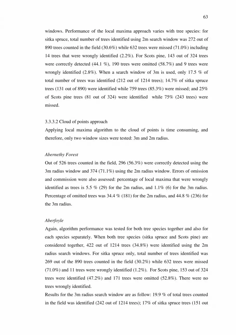
63
windows. Performance of the local maxima approach varies with tree species: for
sitka spruce, total number of trees identified using 2m search window was 272 out of
890 trees counted in the field (30.6%) while 632 trees were missed (71.0%) including
14 trees that were wrongly identified (2.2%). For Scots pine, 143 out of 324 trees
were correctly detected (44.1 %), 190 trees were omitted (58.7%) and 9 trees were
wrongly identified (2.8%). When a search window of 3m is used, only 17.5 % of
total number of trees was identified (212 out of 1214 trees); 14.7% of sitka spruce
trees (131 out of 890) were identified while 759 trees (85.3%) were missed; and 25%
of Scots pine trees (81 out of 324) were identified while 75% (243 trees) were
missed.
3.3.3.2 Cloud of points approach
Applying local maxima algorithm to the cloud of points is time consuming, and
therefore, only two window sizes were tested: 3m and 2m radius.
Abernethy Forest
Out of 526 trees counted in the field, 296 (56.3%) were correctly detected using the
3m radius window and 374 (71.1%) using the 2m radius window. Errors of omission
and commission were also assessed: percentage of local maxima that were wrongly
identified as trees is 5.5 % (29) for the 2m radius, and 1.1% (6) for the 3m radius.
Percentage of omitted trees was 34.4 % (181) for the 2m radius, and 44.8 % (236) for
the 3m radius.
Aberfoyle
Again, algorithm performance was tested for both tree species together and also for
each species separately. When both tree species (sitka spruce and Scots pine) are
considered together, 422 out of 1214 trees (34.8%) were identified using the 2m
radius search windows. For sitka spruce only, total number of trees identified was
269 out of the 890 trees counted in the field (30.2%) while 632 trees were missed
(71.0%) and 11 trees were wrongly identified (1.2%). For Scots pine, 153 out of 324
trees were identified (47.2%) and 171 trees were omitted (52.8%). There were no
trees wrongly identified.
Results for the 3m radius search window are as follow: 19.9 % of total trees counted
in the field was identified (242 out of 1214 trees); 17% of sitka spruce trees (151 out

64
of 890) were identified while 739 trees (83%) were missed; and 28.1 % of Scots pine
trees (91 out of 324) were identified while 71.9% (233 trees) were missed.
Table 3.5 (Discussion) and Figures 3.12 and 3.13 summarise the results presented
above.

65
Abernethy Forest
0
10
20
30
40
50
60
70
80
90
100
2m radius 3m radius 2m radius 3m radius
Cloud of Points Canopy Height Model
Detected (%)
Correct (%)
Error of omission (%)
Error of commission (%)
Figure 3.12: Bar chart showing percentage of correctly detected trees when applying local maxima
algorithm to cloud of points (left) and canopy height model (right), and using 2m-radius and 3m-
radius search windows. Data for Scots pine only, Abernethy Forest, Scotland.
Aberfoyle Forest
0
10
20
30
40
50
60
70
80
90
100
2m radius 3m radius 2m radius 3m radius
Cloud of Points Canopy Height Model
Detected (%)
Correct (%)
Error of omission (%)
Error of commission (%)
Figure 3.13: Bar chart showing percentage of correctly detected trees when applying local maxima
algorithm to cloud of points (left) and canopy height model (right), and using 2m-radius and 3m-
radius search windows. Data for Scots pine only Aberfoyle Forest, Scotland.

66
Figure 3.14: Results of the application of the local maxima algorithm to the cloud of points using a
circular search window of 2 m-radius. Red dots and blue rectangles represent tree tops and plots
respectively. Abernethy Forest, Scotland
Figure 3.15: Results of the application of the local maxima algorithm to the cloud of points using a
circular search window of 2 m-radius. Red dots and blue rectangles represent tree tops and plots
respectively. Aberfoyle Forest, Scotland
67
3.3.4 LiDAR 90th
and 95th
percentiles and mean tree height
Mean tree height at the plot level was compared to 90th
and 95th
percentile LiDAR
height and results are presented below:
Abernethy Forest
Both LiDAR 90th
and 95th
percentile height produced strong correlations with field
mean tree height (r=0.91 and r=0.92 respectively, n= 32, P< 0.001). RMSE was 2.7m
and 2.6m respectively and mean difference 2.2m and 2.0m.
Linear regression was also investigated. Results show that both LiDAR 90th and 95th
percentile height are significant predictors and explains 84% and 83% respectively of
variation in mean tree heights at the plot level (n=32, P< 0.001; Figures 3.16 &
3.17).
Aberfoyle Forest
Correlation between field mean tree height and LiDAR 90th
and 95th
percentile
respectively was also assessed for Aberfoyle. Both LiDAR 90th
and 95th
percentile
height produced strong correlations with field mean tree height (r=0.91 and r=0.94
respectively, n=56, P< 0.001. RMSE was 4.4m and 2.6m respectively and mean
difference 3.3m and 1.3m.
Linear regression was also investigated. Results show that both LiDAR 90th
and 95th
percentile height are significant predictors and explains 82.4% and 88.3%
respectively of variation in mean tree heights at the plot level (n=56, P< 0.001;
Figures 3.18 & 3.19)

68
Figure 3.16: Linear regression between LiDAR 90th
percentile and field mean tree height. LiDAR
90th
percentile explains 84% of variance in field mean tree height at the plot level
(P< 0.00, n=32) Abernethy Forest, Scotland
Figure 3.17: Linear regression between LiDAR 95
th percentile and field mean tree height. LiDAR
95th
percentile explains 83% of variance in field mean tree height at the plot level
(P < 0.00, n=32) Abernethy Forest, Scotland

69
Figure 3.18: Linear regression between LiDAR 90
th percentile and field mean tree height. LiDAR
90th
percentile explains 82.4% of variance in field mean tree height at the plot level
(P<0.00, n=56) Aberfoyle Forest, Scotland
Figure 3.19: Linear regression between LiDAR 95
th percentile and field mean tree height. LiDAR
95th
percentile explains 88.3% of variance in field mean tree height at the plot level
(P< 0.00, n=56). Aberfoyle Forest, Scotland

70
3.4 Discussion
3.4.1 Digital Terrain Model
LiDAR DTMs at Abernethy and Aberfoyle were compared to OS DTMs to assess
whether gross systematic errors could be detected and, if possible, whether this error
could be attributed to LiDAR or OS DTM.
In the case of Abernethy Forest, mean difference between the two DTMs was 2.0 m,
and was found to be significantly different from zero suggesting the presence of
systematic error. A large “flat” area (i.e. no variation in elevation) was detected in
the OS DTM (Figure 3.5) and all outliers (i.e. points where the difference between
both DTMs was higher than +/-5m) fall within that area, suggesting that these
outliers are due to poorer quality of the OS DTM.
Despite the irregularities detected in the OS DTM, the strong correlation between
both DTMs (r= 0.998) suggest that height variations are well represented.
Furthermore, mean difference (2.0m) matches results from previous studies: Gaulton
(2008) assessed the accuracy of LiDAR DTM (created within FUSION) in forested
areas of the UK. A number of reference points distributed over five different
woodlands located in Wales and Scotland were used. In four of these sites, elevation
was measured in the field using a total station; for the fifth site, LiDAR derived
DTM was compared to OS DTM as no accurate field measurements of elevation
were available. Mean difference in meters between LiDAR and field measured
elevations was 0.06, 0.58, -0.94, -1.80, and -2.08 for the fifth site. This last value
(i.e.-2.08m) corresponds to the difference between LiDAR and OS DTM (Gaulton,
2008).
In the case of Aberfoyle Forest, mean difference between LiDAR and OS DTM (-
0.19m) was much lower than for Abernethy and was not significantly different from
zero. Furthermore, the strong correlation between both DTMs (r= 0.999) indicates
that variations in height are well represented. No obvious explanation was found for
the presence of outliers (i.e. differences between OS and LiDAR DTM larger than
+/-5m). Since the results of the assessment were highly satisfactory (i.e. low mean
difference and high correlation) these outliers were not further investigated.

71
3.4.2 Canopy Cover
The discussion focuses on Scots pine results only as this is the key tree species for
this research.
Although canopy cover and canopy closure have been frequently used as
synonymous, both are different measures of canopy density and mean canopy closure
over a given area might not be correlated to mean canopy cover over the same area
(Jennings et al., 1999). Canopy closure has been traditionally associated with
ecological applications such as habitat assessment and monitoring (Paletto and Tosi,
2009). Moreover, previous studies that have investigated habitat preferences of
arboreal squirrel have found a positive relationship between canopy closure and
squirrels presence (Smith and Mannan, 1994; Nelson et al., 2005). On the other
hand, remotely sensed data allow for a simple and direct estimation of canopy cover.
However, due to the narrow angle of view (sensor scan angle), if canopy closure is to
be estimated using LiDAR remote sensed, a more complex approach which includes
in situ data and regression models needs to be developed (Korhonen et al., 2011).
To determine the extent to which LiDAR canopy cover could be used as a surrogate
for canopy closure measured in the field to assess habitat suitability for red squirrels
in this project, the correlation between mean canopy cover and mean canopy closure
at the plot level was assessed. In general it was observed that canopy closure values
were higher than canopy cover values, the reason for this being that canopy closure
measured with the spherical densiometer, which has a wider angle of view, reflects
trees that are not only in vertical direction (Korhonen et al., 2011)
When the correlation between both variables was assessed, the main conclusions
were: Correlation between canopy closure and canopy cover is strong and Spearman
correlation coefficients (rs) are similar when a) all Scots pine plots at Abernethy
Forest are considered (rs =0.65, n=32, P< 0.00); b) when only Scots pine plots at
Aberfoyle Forest are considered (rs =0.75, n=20, P< 0.00) and c) when all Scots pine
plots -from both study areas- are considered (rs =0.71, n=52, P< 0.00). Correlation
decreased when only sitka spruce plots at Aberfoyle are considered for the analysis
(rs =0.41, n=36, P< 0.015). These results support previous research carried out by
Cook et al. (1995) who suggest that relationship between canopy cover and canopy
closure is species dependant.
The difference between mean canopy cover and mean canopy closure was calculated
for each plot. Plots with differences >30% were analysed individually:
72
Abernethy Forest: Plots 10, 12 13 and 14 at Abernethy Forest were all located in a
semi-natural stand, and tree densities in these plots were relatively low, ranging from
5 to 12 trees. The large difference at these plots could therefore be explained by the
fact that the difference between canopy cover and canopy closure increases as
canopy density decreases (Cook et al., 1995). In the case of plot number 2 (diff =
49.8%, Table B.3, Appendix B) it was located within a stand where felling activities
were being carried out at the time the stand was being surveyed. Therefore, it is
possible that trees in this particular plot have been felled between the time when the
plot was surveyed and that when LiDAR data was acquired.
Aberfoyle Forest: 3 plots out of 20 (if only Scots pine plots are considered) present a
difference larger than 30% (39, 43 & 45, Table B.4, Appendix B). In all cases,
LiDAR canopy cover is lower than field canopy closure and the 3 plots are located
near the boundaries of the forest. Plots locations in the field were recorded using a
GPS with accuracy of +/- 1m to 5m. Thus, a miss-match between LiDAR and field
plots can occur – which would lead to LiDAR canopy cover being, for example,
underestimated if part of the plot was located outside the boundary of the forest due
to an error in geolocation.
It is important to highlight here that field canopy closure measurements show low
variability: mean percentage canopy closure ranges from 61% to 93%, while mean
percentage canopy cover (LiDAR) ranges from 11.7% to 95.7 %. Spherical
densiometers have been criticised for their poor resolution and weaker sensitivity to
relatively large variations in canopy closure (Jennings et al. 1999, Cook et al, 1995).
For example, a study carried out by Cook et. al, (1995) showed that moosehorn
estimates from 50% to 95% corresponded to densiometer estimates from 80% to
95%. Nonetheless, spherical densiometers are still widely used as they provide a
more objective approach to visual assessments (Jennings et al. 1999).
Despite spherical densiometer limitations, correlation between LiDAR mean canopy
cover and field mean canopy closure at the plot level is strong (rs=0.71) when only
Scots pine is considered. This matches results from a previous study carried out by
Rosette et. al. (2009) which reports strong correlation between canopy cover derived

73
from airborne LiDAR and canopy closure measured in the field using hemispherical
photography (r=0.77). Results obtained in this study support the use of LiDAR
canopy cover as a surrogate of field canopy closure to assess forest stand
characteristics and therefore red squirrels habitat quality.
3.4.3 Individual tree delineation
The local maxima algorithm was applied to both the canopy height model (CHM)
and the cloud of points. From the results obtained – summarised in Table 3.5- it can
be concluded that the best performance is reached when applying the local maxima
algorithm to the cloud of points with a circular search windows of 2m-radius
(Figures 3.14 & 3.15). A combination of a) higher percentage of trees correctly
detected (71.1% at Abernethy, 47.2 at Aberfoyle); b) lower percentage of omitted
trees (34.4% at Abernethy, 52.8% at Aberfoyle) and c) low percentage of local
maxima wrongly identified as tree tops (5.5% at Abernethy, 0% at Aberfoyle) was
achieved.
Accuracy of individual tree identification using local maxima approach ranges from
75% to 128% (Gaulton, 2008; García et al., 2007; Table 3.6). Therefore, the overall
percentage of trees correctly identified at Abernethy (71.1%) is not far from the
range of values that were found in the literature.
Table 3.5: Percentage of number of trees corrected detected applying local maxima
technique to cloud of points and to canopy height modes, using 2m-radius and 3m-radius
search windows.
Abernethy Forest Cloud of Points Canopy Height Model
Windows search size � 2m radius 3m radius 2m radius 3m radius
Detected trees (%) 403 (76.6) 302 (57.4) 417 (79.3) 326 (62)
Correct (%) 374( 71.1) 296 (56.3) 366 (69.6) 315 (59.9)
Error of omission (%) 181 (34.4) 236 (44.8) 211(40.1) 222(42.2)
Error of commission (%) 29 (5.5) 6 (1.1) 51 (9.7) 11(2.1)
Aberfoyle Forest Cloud of Points Canopy Height Model
Windows search size � 2m radius 3m radius 2m radius 3m radius
Detected trees (%) 153 (47.2) 91 (28.1) 152 (46.9) 81(25)
Correct (%) 153 (47.2) 91 (28.1) 143(44.1) 81(25)
Error of omission (%) 171 (52.8) 233 (71.9) 190 (53.7) 243 (75)
Error of commission %) 0 (0) 0 (0) 9 (2.8) 0 (0)

74
Error of commission and omission can be caused by search-window size being too
small or too large respectively. Overlapping crowns in dense stands also cause error
of omission (Popescu et. al., 2003). In this study, lower accuracies at the plot level
were achieved in plots with high tree densities, which suggest that errors of omission
are more likely due to overlapping crowns. These findings support previous research
by Vauhkonen et al. (2012) who found that the number of trees successfully detected
under different forest types was strongly dependent on tree density and spatial
distribution of trees (i.e. clustering).
Using a smaller window size (i.e. 1m) would probably increase the number of trees
correctly detected in young Scots pine stands but would also presumably increase the
error of commission (i.e. wrongly detected trees) in mature stands. In Aberfoyle, all
sampled Scots pine stands were composed of mature trees, while in Abernethy, only
1 out of 4 stands was composed of young trees. On the other hand, only a small
percentage of local maxima (5.7 % at Abernethy, 0% at Aberfoyle) were wrongly
identified as trees, which is likely due to more than one local maxima allocated to the
same crown. This suggests that only in a few cases the search window was larger
than the tree crowns, and therefore, the 2m-radius window size was considered to be
a good balance.
The use of a variable-size search window -where the window-size would be a
function of the tree height- could potentially increase the number of trees accurately
detected. This approach used in combination with local maxima produced an
accuracy of 89.3% (García et al, 2007; Table 3.6). One limitation of this technique is
that accurate allometric relationships between tree height and crown size are needed.
Furthermore, it is not clear whether –in the study mentioned above- the accuracy
increased due to the variable-size search window or to the higher pulse densities (3-4
pulses/m2).
LiDAR data resolution (i.e. point’s density) has a strong influence on individual trees
delineation and high densities are needed for effective and robust individual trees
detection (Lee et al, 2010; Gaulton, 2008; Gaulton & Malthus, 2010; Vauhkonen et
al., 2012). Higher proportions of total number of trees have been detected using laser
resolution higher than 5 pulses/m2 (Holmgren, 2004) Table 3.6 shows a summary of
accuracy achieved in previous studies and LiDAR data resolution (pulses/m2) used.
The number of trees correctly detected seems to depend more on the data resolution

75
than on the approach itself. This explains the low percentage of correctly detected
trees in Aberfoyle (47.2 %, 1 pulses/m2) in comparison to Abernethy (71, 1%; 2
pulses/m2). Gaulton and Malthus (2010) report accuracies of 78% when using
LiDAR data densities of 1 pulse/m2
in spruce plantations in Aberfoyle. However, the
current study suggests that at least data densities of 2 pulses/m2
are needed to
achieve relatively good results (71.1%) in pine stands.
Finally, as validation was not performed based on individual tree locations but on
number of trees per plot, errors in geolocation could have also contributed to errors
in number of detected trees.
Table 3.6: Summary of accuracy achieved and LiDAR data resolution (pulses/m2) used for
delineating trees in previous studies
Detected trees (%)
LiDAR pulses/m
2
Approach
Reference
75-79 1-2 Local maxima Gaulton, 2008; Doo-Ahn Kwak et al, 2007
80 2 GIS morphological tools (contours around crowns)
Koukoulas et al.; 2005
77.9 3-4 Watershed Garcia, et. al.,2007
89.3 3-4 Local maxima (variable windows size)
Garcia, et. al.,2007
83 (dominant trees); 39.5 (total trees)
10 Local maxima Maltamo et. al., 2004
84 11 Local maxima Gaulton , 2008
95 12 to 18 Local maxima Lee et al, 2010
128 3-4 Local maxima + crown segmentation
Garcia, et. al.,2007
3.4.4 LiDAR 90th
and 95th
percentiles as estimators of mean tree height
Based on previous research (see Introduction) the relationship between mean field
tree height and 90th
and 95th
percentiles of LiDAR height was investigated.
Both correlation and linear regression were explored to see which of these two
LiDAR metrics would best match mean tree height at the plot level. Previous studies
(for example, Hopkinson et al, 2008; Holmgren, 2004) investigated the relationship
between LiDAR metrics and field tree height for heterogeneous forest without

76
distinction of tree species. Thus, for Aberfoyle, all plots (i.e. sitka spruce and Scot
pine) were assessed together.
Results are summarised in Table 3.7. In both study areas, strong correlations exist
between both LiDAR 90th
and 95th
, and mean field height at the plot level.
Furthermore, 90th
and 95th
percentiles explain a high percentage of variation of mean
tree height. In both cases, correlation and regression coefficients as well as root mean
square error suggest a better performance of 95th
percentile as estimator of mean tree
height. These results do not match results from a previous study carried out by
Hopkinson et al (2008) where correlation with mean field tree height was slightly
stronger for LiDAR 90th
percentile (r=0.80, n=38) than for 95th
percentile (0.79,
n=38).
Table 3.7: Correlation and regression between LiDAR 90th and 95
th percentiles and mean
tree height at the plot level, Abernethy and Aberfoyle Forests, Scotland.
90th percentile Vs. mean tree height
95th percentile Vs. mean tree height
Correlation Regression Correlation Regression
Abernethy n=32
r=0.91 p-value<0.000 RMSE= 2.7
R2 = 84%
p-value<0.000 r=0.92 p-value<0.000 RMSE= 2.6
R2 = 83%
p-value<0.000
Aberfoyle n=56
r=0.91 p-value<0.000 RMSE= 4.4
R2 =82.4%
p-value<0.000 r=0.94 p-value<0.000 RMSE= 2.6
R2 =88.3%
p-value<0.000
Doce et al (2008) suggested that the effectiveness of LiDAR percentiles of height as
estimators of stand canopy heights is species dependent. In this study, correlation
parameters were very similar for Abernethy Forest - where all plots consist of Scots
pine only, and Aberfoyle – where 20 plots (out of 56) are Scots Pine and the rest are
sitka spruce. This would suggest that, at least for these study areas, tree species
composition does not affect the performance of the approach. However, if the
approach is intended to be used in different forest types (i.e. different species or
mixed stands) it should be tested in each case.

77
CHAPTER 4
GLM implementation using LiDAR derived explanatory variables
_________________________________________________________
The importance of forest structural parameters for red squirrels habitat mapping was
addressed in Chapter 2. A General Linear Model (GLM) was used to relate the
number of cones stripped by squirrels to mean canopy closure, mean tree height and
total number of trees at the plot level. Chapter 3 introduced LiDAR remote sensing
as a possible tool to extrapolate the analysis to the whole study areas. Methodologies
to derive canopy cover (as a surrogate for field canopy closure), number of trees and
tree height were described and results of accuracy assessment presented and
discussed. The main aim of this Chapter is to implement the GLM using LiDAR
derived explanatory variables in both study areas and to assess LiDAR-based model
performance. The latter was achieved by performing a correlation between LiDAR-
predicted and field-predicted number of cones stripped by squirrels. Moderate to
high Spearman rank correlation coefficients (0.59 for Abernethy and 0.54 for
Aberfoyle) suggest that LiDAR performs relatively well over the extent of the study
areas. Finally, based on the GLM and using LiDAR data, habitat suitability maps
were generated. Results suggest that when forest structure is considered, only 27% of
the total forest area at Abernethy and 37% at Aberfoyle are suitable for red squirrel.
Implications for management are discussed.
_________________________________________________________
4.1 Introduction
Forest structure is an important factor explaining wildlife distribution and species
habitat preferences (Clawges et. al. 2008). Several statistical models that relate the
presence or abundance of specific animal species (i.e. birds) to variations in
vegetation structure have been developed. However, since vegetation structural data
collection at broad scale is both prohibitively expensive and time consuming, these
models and studies have often been focussed on small areas (Bradbury et. al., 2005;
Clawges et. al. 2008; Martinuzzi et.al. 2009).

78
Passive (i.e. optical) remote sensing has been widely used to assess aspects of
forested habitats over large areas but has not been able to successfully characterize
and describe vertical forest structure (Lefsky et. al., 2002; Bradbury et al, 2005;
Turner et al, 2003). Active remote sensing, in particular LiDAR, can be used to
directly measure structural characteristics of forest stands such as canopy cover,
canopy height and height variability (Patenaude et al. 2004, Bradbury et al., 2005;
Clawges et. al. 2008; Martinuzzi et al. 2009).
Several researchers have used LiDAR remote sensing to assess habitat quality for
different species with different degrees of success. Clawges et al. (2008) used
LiDAR data to investigate the relationship between remote sensing derived
vegetation indices, diversity and density of birds in South Dakota (USA). They
calculated three LiDAR derived vegetation indices: shrub density, which is
calculated using all returns between 0.5m and 2m; foliage height diversity which is
the proportion of returns at different levels ranging from 0 to 20m; and total
vegetation volume which is the total number of LiDAR returns above 2m. Their main
findings show that, out of the 43 bird species surveyed, the relative densities of two
species (dark-eyed juncos Junco hyemalis and warbling vireos Vireo gilvus) were
strongly correlated with LiDAR shrub density (r= 0.63, P<0.01, n=51 and r=0.59,
P<0.01, n=51 respectively), while total bird species density was significantly but not
strongly correlated with LiDAR total vegetation volume (r= 0.33, P< 0.017, n=51).
LiDAR remote sensing has also been used to assess habitat quality for great tits
(Parus major) and blue tits (Parus caeruleus) in Monks Wood, UK. Hill et al. (2004)
found that great tits average nestling body mass increased with mean vegetation
height estimated from LiDAR data; while blue tits average nestling body mass
decreased with LiDAR derived mean vegetation height. Average nestling body mass
is a measure of breeding success which results from the combination of food
abundance and adults foraging efficiency, and therefore reflects habitat quality.
Goetz et al. (2010) investigated the applicability of LiDAR remote sensing to habitat
quality prediction for black-throated blue warbler (Setophaga caerulescens) in
Hubbard Brook Experimental Forest, USA. Canopy height, height of median return,
canopy complexity (computed taking into account number and amplitude of peaks in
a waveform), and vertical distribution ratio (related to the distance between the
canopy height and the height of the median return: the shorter the distance, the lower
the vertical distribution ratio) were derived from LiDAR data. LANDAT ETM data

79
was also used to generate an image of seasonal NDVI change (difference between
leaf-on and leaf-off NDVI). A decision tree method was used to model the
distribution and abundance of the bird species and results showed that the variables
derived from remote sensing accounted for 47% of variation in birds’ data: seasonal
NDVI difference, canopy height and vertical complexity were the most significant
predictors.
Lesak et al. (2011) used step regression to assess the relationship between a number
of LiDAR metrics and songbird species richness in Baraboo Hills, USA. LiDAR-
derived variables used for this study were mean and coefficient of variation of return
height, number of non-ground returns, proportion of returns within different height
intervals, and 10% quantiles of height (i.e. 10, 20, 30...100). All variables were
computed for the same 15m-radius plots where bird surveys were carried out. Several
models were run and the best performance was achieved by a combination of 50th
,
60th
and 100th
height percentile, and the proportion of returns within a 10 m layer in
the middle (i.e. between ground elevation and maximum tree height). This model
explained 21.6% of variability in songbird species richness.
LiDAR remote sensing has also been used to improve habitat modelling for
Capercaillie (Tetrao urogallus; Alps, Switzerland) by incorporating vegetation
vertical structure. Graf et al. (2009) used relative fraction of tree canopy, mean and
standard deviation of canopy height, and density of tree canopy edges (defined as
contour length at 10, 20m and 30 m height) derived from LiDAR data at a spatial
resolution of 125m (i.e. cell size = 125m). A general linear model (GLM) was used
to predict presence/absence of the species, with the above mentioned LiDAR metrics
as the explanatory variables. Model predicted presence of the species in 36% of the
study area and absence in the rest, where presence and absence of the species were
assumed to represent suitable and unsuitable habitat respectively.
Although mostly used to assess habitat for birds, LiDAR data have also been used to
improve habitat modelling for mammals. For example, Nelson et al. (2005) used tree
height and canopy cover to assess habitat quality for the endangered Delmarva fox
squirrel (Sciurus niger; DFS) in the Delmarva Peninsula, USA. LiDAR flight lines
were split into segments of 40m and average canopy height and average canopy
cover were calculated for each segment. Knowing that the squirrel prefers tall trees
and dense canopies, those areas with mean tree height > 20m and mean canopy cover

80
> 80% were selected. Out of the 32 identified sites, 25 (78%) were actually suitable
habitat for the species.
With respect to the red squirrel in the UK - the focus of this research- suitable habitat
or habitat quality has been mainly related to tree species composition and food
availability (e.g. Gurnell 1983, 1987; Lurz et al. 2000). While the relationship
between red squirrel habitat use and forest structural factors, such as canopy
connectivity, tree densities and height heterogeneity has been suggested (e.g. Gurnell
et al. 2002) it has not yet been quantified. In order to better understand and quantify
this relationship, in this study data on forest structure and red squirrel food remains
were collected during two field seasons carried out in a semi-natural Scots pine
(Pinus sylvestris) forest (Abernethy) and a Scots pine plantation (Aberfoyle). A
general linear model (GLM) was then used to relate key stand structural variables to
squirrel feeding behaviour and thus patch selection. Results showed that mean
canopy closure, total number of trees and mean tree height (at the plot level) were
significant predictors and explained 43% of the variability in the number of cones
stripped by squirrels (P < 0.013, 0.031 and 0.058 respectively, n=52). Details on data
collection and analysis are presented in Chapter 3 and in Flaherty et al. (2012).
These results highlight the importance of considering structural characteristics of
forest stands in the forest design for red squirrels. However, evaluating and
monitoring vegetation structure at the forest level is expensive and time consuming.
Hence, for management purposes these results advocate the need for methods to
extract and utilise structural data (notably canopy closure and total number of trees)
to derive habitat suitability information over large forest areas. LiDAR remote
sensing can be used to retrieve the three variables found to significantly influence red
squirrel feeding behaviour (namely canopy cover, tree height and number of trees).
The aim of this Chapter is to estimate and map habitat suitability over the whole
study area using LiDAR derived variables and the GLM presented in Chapter 3. For
a review of techniques used to retrieve these forest structural variables as well as
validation performed by comparing LiDAR derived products to data collected in the
field, please consult Chapter 3. To achieve the aims of this Chapter, the following
objectives will be addressed:

81
1. To ensure that only the error resulting from LiDAR is accounted for (excluding
that inherent from the original GLM), results from a leave-one-out cross
validation approach will be presented. This enables field-based predictions of the
number of cones stripped by squirrels to be generated. These predictions, rather
than the raw field number of stripped cones, are used to validate LiDAR
predictions.
2. To assess the number of cones stripped by squirrels at wider scales, the GLM will
be implemented using LiDAR data
3. The accuracy of the LiDAR predicted number of stripped cones will then be
assessed, and finally,
4. Habitat suitability maps for both study areas and based on LiDAR data and the
GLM will be produced.
In the next section a brief overview of the study sites is presented along with the
methodology adopted to achieve the objectives listed above.
4.2 Methodology
4.2.1 Study Areas
Fieldwork was carried out at Abernethy Forest in October 2009 and at Aberfoyle in
May 2010.
Abernethy Forest (57° 15’ N, 3° 40’ W) is owned and managed by the Royal Society
for the Protection of Birds (RSPB) and lies between 200 m and 500 m altitude with a
total area of 28 km 2 (Summers and Proctor, 1999). Two thirds of the forest (19
km 2 ) is native forest and one third is plantation. The dominant tree species is Scots
pine.
Aberfoyle (56° 10” N, 4° 22” W) is managed by the Forestry Commission Scotland.
The forest is part of the Loch Lomond and Trossachs National Park, located in the
west of Scotland, approximately 25 km North-West of Glasgow. Total forest area
estimated from Forestry Commission stock maps is slightly less than 12000 ha. Tree
species present in the forest are predominantly conifers and include Scots pine, sitka
spruce (Picea sitchensis), lodge pole pine (Pinus contorta) and Norway spruce
(Picea abies). A number of semi-natural stands consisting of oak (Quercus petraea),

82
birch (Betula spp.), alder (Alnus glutinosa) and ash (Fraxinus excelsior) are also
present. Scots pine covers 943.5 ha of the total forest area (McInerney et. al., 2010).
Both forests are home to the native red squirrel. Further details on both study areas
are provided in Chapter 2.
4.2.2 Field-based GLM validation
GLM development
A general linear model (GLM) was developed to relate key stand structural variables
to squirrel feeding behaviour. The resulting GLM is presented below:
SC = -6.5 + (0.083) CC + (0.018) NT + (0.083) TH
Where SC is total number of stripped cones, CC is mean canopy closure, NT is total
number of trees and TH is mean tree height (See Chapter 2 for more details).
GLMs are used when variables are not normally distributed and variance is not
constant (Crawley, 2007). GLMs use a link function to relate predicted values to
linear predictors. In the case of Poisson error structure, which is commonly used for
count data, the default link function is log (e). In order to obtain values on the scale
of the original dependent variables, predictions from the model need to be back-
transformed (antilog) before results can be interpreted (Crawley, 2007).
GLM Validation
Cross validation is used to assess model performance. The approach relies on making
new predictions using data not used in the development of the model. Hold-out is the
simplest way to perform cross-validation. It consists of splitting the data into two
datasets: one for model fit (training dataset) and one for model validation (testing
dataset). A key disadvantage of this approach is that evaluation depends heavily on
which data points are used for training and which ones are used for testing.
Moreover, data might not be enough to keep part of it for testing. A more exhaustive
version of this method is referred to as leave-one-out (LOO) cross-validation (Arlot
& Celisse, 2010). In this case, the predictive power of the model is assessed as
follows:

83
(a) Considering n observations, observation i is left out and the model is fit using
the rest of the data.
(b) The model is then run and a prediction is made for the omitted observation
(c) The error is computed (ei = observed yi - predicted yi ).
(d) This procedure is repeated for each individual observation. As a result, the
model is run n times.
(e) Model performance is ultimately assessed by exploring the correlation
between observed data (i.e. data collected in the field) and the values
predicted by the model for each data point.
(f) Average or mean square error is then also computed to evaluate the overall
performance of the model (Arlot & Celisse, 2010).
This approach provides an efficient use of the available data, as only one observation
is omitted at each step. One key criticism of the approach is that it can be very time
consuming to implement.
In this study, LOO cross-validation was performed to assess field-based model
performance. The model was expected to provide relative rather than absolute
abundance of stripped cones per plot (Pearce and Ferrier, 2001). In this context this
means that plots with higher numbers of stripped cones would be more suitable than
those with lower numbers of stripped cones. For this reason, and also because
variables were not normally distributed, all correlations were assessed using a
Spearman rank correlation coefficient.
The values predicted by LOO cross-validation (field-predicted stripped cones) were
also used to assess LiDAR performance. This is explained in more detail in the
following sections.
4.2.3 Implementation of GLM using LiDAR
The field measured variables used in the GLM to predict number of cones stripped
by squirrels were replaced by LiDAR derived variables. This enables an assessment
of habitat quality for the whole study areas.
4.2.3.1 LiDAR data acquisition and pre-processing
LiDAR data characteristics are summarised in Table 4.1.
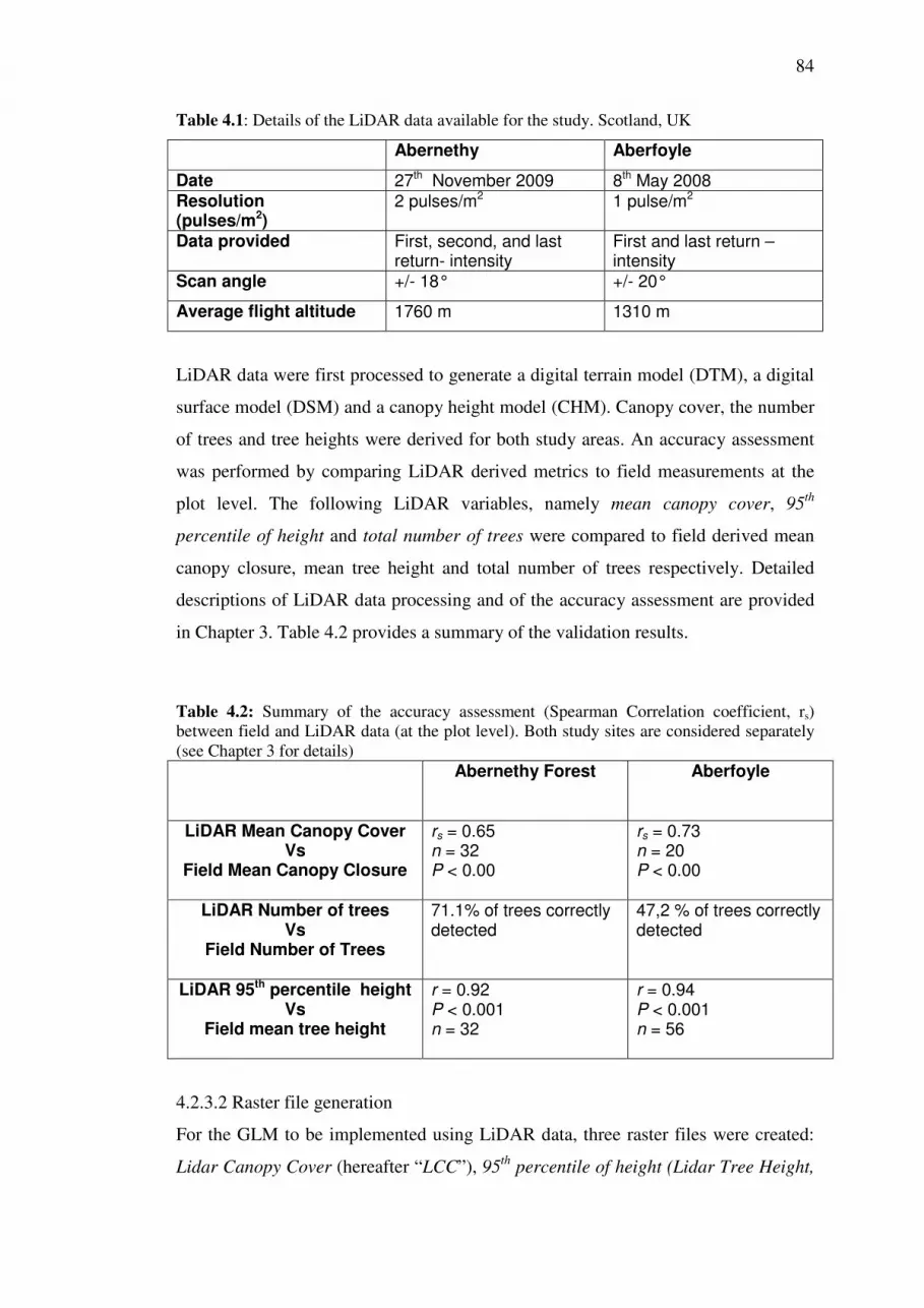
84
Table 4.1: Details of the LiDAR data available for the study. Scotland, UK
Abernethy Aberfoyle
Date 27th November 2009 8th May 2008 Resolution (pulses/m2)
2 pulses/m2 1 pulse/m2
Data provided First, second, and last return- intensity
First and last return – intensity
Scan angle +/- 18° +/- 20°
Average flight altitude 1760 m 1310 m
LiDAR data were first processed to generate a digital terrain model (DTM), a digital
surface model (DSM) and a canopy height model (CHM). Canopy cover, the number
of trees and tree heights were derived for both study areas. An accuracy assessment
was performed by comparing LiDAR derived metrics to field measurements at the
plot level. The following LiDAR variables, namely mean canopy cover, 95th
percentile of height and total number of trees were compared to field derived mean
canopy closure, mean tree height and total number of trees respectively. Detailed
descriptions of LiDAR data processing and of the accuracy assessment are provided
in Chapter 3. Table 4.2 provides a summary of the validation results.
Table 4.2: Summary of the accuracy assessment (Spearman Correlation coefficient, rs)
between field and LiDAR data (at the plot level). Both study sites are considered separately
(see Chapter 3 for details)
Abernethy Forest Aberfoyle
LiDAR Mean Canopy Cover Vs
Field Mean Canopy Closure
rs = 0.65 n = 32 P < 0.00
rs = 0.73 n = 20 P < 0.00
LiDAR Number of trees Vs
Field Number of Trees
71.1% of trees correctly detected
47,2 % of trees correctly detected
LiDAR 95th percentile height Vs
Field mean tree height
r = 0.92 P < 0.001 n = 32
r = 0.94 P < 0.001 n = 56
4.2.3.2 Raster file generation
For the GLM to be implemented using LiDAR data, three raster files were created:
Lidar Canopy Cover (hereafter “LCC”), 95th
percentile of height (Lidar Tree Height,

85
hereafter “LTH”) and Lidar Number of Trees (hereafter “LNT”). For the field-based
GLM, mean values at the plot level were used. To ensure comparability, pixel size
for the LiDAR derived raster files was the same as field plot size (i.e. 14m x 14m).
LiDAR Canopy cover
LCC was computed as the proportion of vegetation returns above a threshold or
height-break for a given cell grid, where
LCC = number of returns > height-break / total number of returns (McGaughey,
2009).
The value used as threshold was the height at which measurements were made in the
field (breast height =1.3 m). The output pixel size was 14m. To compute and extract
LCC, the FUSION software was used (details provided in Chapter 3).
LiDAR Tree Height
The GridMetrics functionality available in FUSION enables the computation of a
series of descriptive statistics for all returns within each cell in the output grid. The
program was used to compute the 95th percentile height value for each of the 14m x
14m cells. The 95th
percentile was used as a surrogate for mean tree height following
my detailed review and validation (Chapter 3). GridMetrics computes percentiles as
follows:
(n-1) p = i + f
Where i is the integer part of (n-1) p; f is the fractional part of (n-1) p, n=number of
observations (in this case, height values per cell) and p is percentile value divided by
100
If f=0, Percentile Value = xi+1
If f>0, Percentile Value = xi+1+f (xi+2 – xi+1) (McGaughey, 2009).
LiDAR Number of trees
Original LiDAR files containing first-return cloud of points (noise removed, see
Chapter 3 for details) were split into smaller more manageable tiles and the local
maxima algorithm was applied to all tiles (using MATLAB 7.12.0). The local
maxima technique identifies the highest return within a moving window by
comparing them to their near neighbours (also described in Chapter 3). To avoid
false detections on the edges of the tiles, overlapping areas (between tiles) were kept.

86
Once the local maxima had been performed those overlapping areas were removed.
The algorithm produces ASCII files containing X, Y coordinates and height of the
identified trees. These files were converted into vector (point) files using ArcGIS
9.3. A polygon (fishnet) composed of 14m x 14m cells was created, LiDAR detected
trees falling within each cell were counted and recorded and a raster file was created
using the “count” field as pixel value. The output file is a raster where each 14m x
14m pixel value represents the number of trees within each square of the fishnet. All
tiles were finally merged together to create one raster file for the whole study area.
Calibrated Number of trees
Unlike the LCC and LTH, the LiDAR number of trees (LNT) was the LiDAR
derived variable with the poorest performance, in particular for Aberfoyle, where
only 47.2 % of the trees were correctly detected. This poor result for Aberfoyle is
probably due to the low spatial resolution of LiDAR data (i.e. 1 pulse/m2 as opposed
to 2 pulses/m2 for Abernethy).
LiDAR spatial resolution can range from an average of 1 pulse/m2 or less (i.e. 0.3 or
0.5) to more than 12 pulses/m2 .Acquiring lower densities LiDAR data allows for
higher flying altitudes and therefore reduces acquisition costs (Evans et al, 2009).
However, higher pulse densities allow for more accurate detection and mapping of
objects on the earth surface, and as discussed in Chapter 3, it also allows for more
accurate detection of individual trees (Lee et al, 2010; Gaulton, 2008).
Given this poor result for Aberfoyle, and acknowledging that the aim of this study is
fundamentally to generate red squirrel habitat suitability maps using only LiDAR
data, I calibrated the LNT using field data (i.e. field counted number of trees) and a
linear regression. While this may appear as a circular argument-as I am using field
data to calibrate LiDAR- the reasoning for doing so is to assess the effects on the
habitat suitability maps of the low spatial resolution of the Aberfoyle LiDAR data,
and to determine if higher density LiDAR data is necessary to improve the accuracy
of the LiDAR predicted number of cones and therefore, of the LiDAR based habitat
suitability maps.
To achieve this aim, the following objectives will be addressed:
• To assess whether the accuracy of the LNT improves when the correction is
applied

87
• To implement the GLM using the LNT as originally derived from LiDAR
(GLM 1) and the calibrated LNT (GLM 2).
• To assess the accuracy of both GLM 1 and GLM 2 using LOO cross-
validation and RMSE (as explained in section 4.2.2 )
Calibration regression
There is evidence that a relationship between number of trees and tree height might
exist, although it depends on other factors such as tree species and yield (Zeide,
1995). With the purpose of improving the calibration regression, I tested whether this
relationship existed in Aberfoyle by incorporating LiDAR 95th
height percentile
(LTH) into the equation. I found that LTH was also a significant predictor of LiDAR
number of trees and that LTH and FNT together explained 57% of the variation in
LiDAR number of trees (P < 0.001, n=20)
The calibration regression is presented below:
LNT = 31.2 - 1.37 LMH + 1.08 FNT
Where LNT is the LiDAR number of trees, LMH is the LiDAR mean height and
FNT is the field number of trees,
This regression was used to calibrate the Aberfoyle LNT and two different habitat
suitability maps were generated (GLM 1 and GLM 2). The LiDAR number of trees
per plot after applying the calibration was compared to the number of trees counted
in the field to assess the performance of the regression.
In the case of Abernethy, the number of trees correctly detected (71.1 %) was
considered to be within the expected range of accuracy as found in the literature
(Gaulton, 2008; Doo-Ahn Kwak et al., 2007; Garcia, et al., 2007) and no correction
was applied.
4.2.3.3 GLM implementation
For Abernethy Forest, the whole LiDAR image was used for the analysis. For
Aberfoyle (based on forest stock maps, Forestry Commission Aberfoyle, 2010) only
forested areas corresponding to Scots pine stands were selected. For both study
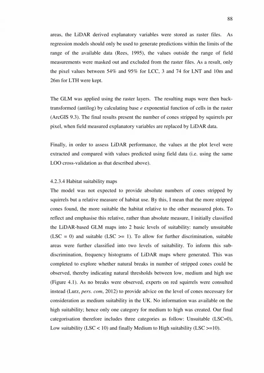
88
areas, the LiDAR derived explanatory variables were stored as raster files. As
regression models should only be used to generate predictions within the limits of the
range of the available data (Rees, 1995), the values outside the range of field
measurements were masked out and excluded from the raster files. As a result, only
the pixel values between 54% and 95% for LCC, 3 and 74 for LNT and 10m and
26m for LTH were kept.
The GLM was applied using the raster layers. The resulting maps were then back-
transformed (antilog) by calculating base e exponential function of cells in the raster
(ArcGIS 9.3). The final results present the number of cones stripped by squirrels per
pixel, when field measured explanatory variables are replaced by LiDAR data.
Finally, in order to assess LiDAR performance, the values at the plot level were
extracted and compared with values predicted using field data (i.e. using the same
LOO cross-validation as that described above).
4.2.3.4 Habitat suitability maps
The model was not expected to provide absolute numbers of cones stripped by
squirrels but a relative measure of habitat use. By this, I mean that the more stripped
cones found, the more suitable the habitat relative to the other measured plots. To
reflect and emphasise this relative, rather than absolute measure, I initially classified
the LiDAR-based GLM maps into 2 basic levels of suitability: namely unsuitable
(LSC = 0) and suitable (LSC >= 1). To allow for further discrimination, suitable
areas were further classified into two levels of suitability. To inform this sub-
discrimination, frequency histograms of LiDAR maps where generated. This was
completed to explore whether natural breaks in number of stripped cones could be
observed, thereby indicating natural thresholds between low, medium and high use
(Figure 4.1). As no breaks were observed, experts on red squirrels were consulted
instead (Lurz, pers. com, 2012) to provide advice on the level of cones necessary for
consideration as medium suitability in the UK. No information was available on the
high suitability; hence only one category for medium to high was created. Our final
categorisation therefore includes three categories as follow: Unsuitable (LSC=0),
Low suitability (LSC < 10) and finally Medium to High suitability (LSC >=10).
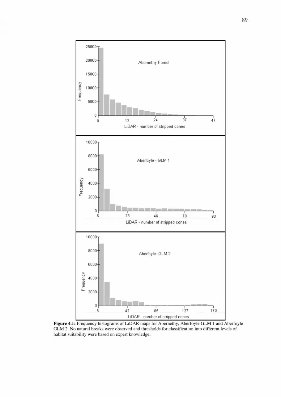
89
Figure 4.1: Frequency histograms of LiDAR maps for Abernethy, Aberfoyle GLM 1 and Aberfoyle
GLM 2. No natural breaks were observed and thresholds for classification into different levels of
habitat suitability were based on expert knowledge.

90
4.3 Results
4.3.1 Field-based GLM validation
A Spearman rank correlation between the field-collected and the field-predicted
(LOO cross-validation) cones stripped by squirrels was assessed for all data together
(i.e. Abernethy plus Aberfoyle). Results show a moderate performance of the field-
based model (rs =0.40; P <0.004, n=52, RMSE = 20, Figure 4.2, Table C.3,
Appendix C).
Figure 4.2: The correlation between the field-collected (Observed SC) and the field-predicted
(Predicted SC) number of stripped cones for all data together (i.e. Abernethy plus Aberfoyle). Results
show a moderate performance of the field-based model (rs =0.40; P <0.004, n=52, RMSE = 20,
4.3.2 Implementation of GLM using LiDAR
The field-predicted number of stripped cones was also compared to the LiDAR-
predicted number of stripped cones. LiDAR data acquired at Aberfoyle and
Abernethy had different characteristics (in particular pulse density) which has an
influence in the accuracy of LiDAR derived metrics. Thus, correlations between
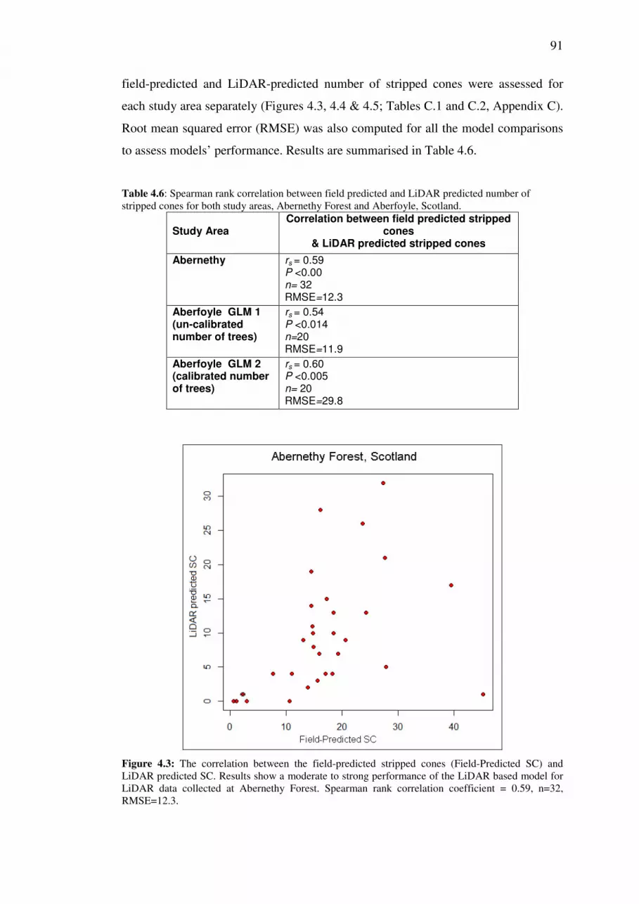
91
field-predicted and LiDAR-predicted number of stripped cones were assessed for
each study area separately (Figures 4.3, 4.4 & 4.5; Tables C.1 and C.2, Appendix C).
Root mean squared error (RMSE) was also computed for all the model comparisons
to assess models’ performance. Results are summarised in Table 4.6.
Table 4.6: Spearman rank correlation between field predicted and LiDAR predicted number of
stripped cones for both study areas, Abernethy Forest and Aberfoyle, Scotland.
Study Area
Correlation between field predicted stripped cones
& LiDAR predicted stripped cones
Abernethy
rs = 0.59 P <0.00 n= 32 RMSE=12.3 Aberfoyle GLM 1
(un-calibrated number of trees)
rs = 0.54 P <0.014 n=20 RMSE=11.9 Aberfoyle GLM 2
(calibrated number of trees)
rs = 0.60 P <0.005 n= 20 RMSE=29.8
Figure 4.3: The correlation between the field-predicted stripped cones (Field-Predicted SC) and
LiDAR predicted SC. Results show a moderate to strong performance of the LiDAR based model for
LiDAR data collected at Abernethy Forest. Spearman rank correlation coefficient = 0.59, n=32,
RMSE=12.3.

92
Figure 4.4 Correlation between field-predicted and LiDAR-predicted number of stripped cones using
the un-calibrated LNT (GLM 1) Spearman rank correlation coefficient = 0.54, n=20, RMSE= 12.2.
Aberfoyle Forest, Scotland
Figure 4.5: Correlation between field-predicted and LiDAR predicted number of stripped cones (SC)
using the calibrated LNT(GLM 2) Spearman rank correlation coefficient = 0.60, n=20, RMSE=29.8
Aberfoyle Forest, Scotland

93
4.3.2.1 Calibration of Aberfoyle number of trees
Considering all plots, a total of 354 trees were detected (109%). Out of 324 trees
counted in the field, 243 (75%) were correctly detected, 81 (25%) were omitted, and
108 (33%) were wrongly detected. Accuracy assessments for Abernethy and
Aberfoyle (un-calibrated) are presented in Chapter 3.
4.3.2.2 Habitat suitability maps
LiDAR-predicted number of cones stripped by squirrels (i.e. GLM map pixel values)
ranged from 0 to 48 at Abernethy, 0 to 93 at Aberfoyle GLM 1 and 0 to 170 for
GLM 2. LiDAR-based GLM maps were classified into three habitat suitability
levels: Unsuitable, Low suitability and Medium-to-High suitability.
Sizes of the areas falling within the different categories were calculated for all the
maps: at Abernethy, 30% of the area was classified as Unsuitable and 70% as
Suitable, of which 43% as Low and 27% as Medium-to-High suitability. For
Aberfoyle GLM 1, 26% was classified as Unsuitable and 74% as Suitable; of which
37% as Low and 37% as Medium-to-High suitability. For GLM 2, 24% was
classified as Unsuitable and 76% as Suitable, of which 29% as Low and 47% as
Medium-to-High suitability.
The size of the areas for both Aberfoyle GLM 1 and GLM 2 were compared to assess
the effects of the correction in number of trees. Results show a significant difference
in the size of the areas (Chi-squared test, p<0.016) with an increase in the size of the
Suitable and Medium-to-high suitability areas as well as a decrease in the Unsuitable
and Low suitability areas when the number of trees is corrected at Aberfoyle (GLM
2). These results are presented in Table 4.7 and Figures 4.6, 4.7, 4.8a & 4.8b.
Table 4.7: Total areas (ha) within each habitat suitability category for both Abernethy and Aberfoyle
forests- Aberfoyle results for both GLM 1 and GLM 2.
Abernethy Aberfoyle
Suitability Level
area (ha) GLM area (ha) GLM 1 area (ha) GLM 2
Unsuitable 352.5 (30%)
93.8 (26%)
87.9 (24%)
Low
492.4 (43%)
132.1 (37%)
101.6 (29%)
Medium to high
319.6 (27%)
133.5 (37%)
169.9 (47%)

94
Figure 4.6: LiDAR derived habitat suitability map, Abernethy Forest, Scotland. Habitat suitability
was classified into 2 categories: Unsuitable and Suitable. Non-data areas (i.e. non forest and areas
outside the range of values observed in the field) are shown in white.

95
Figure 4.7: LiDAR derived habitat suitability map, Abernethy Forest, Scotland. Habitat suitability
was classified into 3 categories: Unsuitable, Low suitability and Medium-to-high suitability. Non-data
areas (i.e. non forest and areas outside the range of values observed in the field) are shown in white.

96
F
igu
re 4
.8a:
LiD
AR
der
ived
hab
itat
suit
abil
ity m
ap (
GL
M 1
), A
ber
foyle
, S
cotl
and
. S
cots
pin
e st
and
s ar
e w
idel
y s
pre
ad i
n A
ber
foyle
and
ther
efo
re i
s d
iffi
cult
to
sho
w d
iffe
rence
s
bet
wee
n d
iffe
rent
mo
del
s/cl
ass
ific
ati
on
s sc
hem
es.
The
who
le s
tud
y a
rea
is s
ho
wn
in t
his
fig
ure
. T
he
larg
est
stan
d (
bla
ck r
ecta
ngle
) has
bee
n z
oo
med
–in
to
sho
w i
n d
etai
l hab
itat
suit
abil
ity c
lass
ific
atio
n i
n F
igure
4.8
b.

97
F
igu
re 4
.8b
: L
arges
t S
cots
pin
e st
and
in A
ber
foyle
Fo
rest
. T
he
dif
fere
nt
mo
del
s/cl
assi
ficat
ions
schem
es
are
sho
w a
s fo
llo
w:
1)
GL
M-1
/2 c
lass
es,
2)
GL
M-1
/3 c
lass
es,
3)
GL
M-2
/2
clas
ses;
4)
GL
M-2
/3 c
lass
es.
No
-dat
a ar
eas
(i.e
. no
n S
cots
pin
e st
and
s, n
o-f
ore
st a
nd
are
as o
uts
ide
the
ran
ge
of
val
ues
ob
serv
ed i
n t
he
fiel
d)
are
sho
wn i
n w
hit
e.

98
4.4 Discussion
4.4.1 Field-based GLM
The first objective of this chapter was to validate the field-based GLM developed in
early stages of this project (see Chapter 2). The results from the LOO cross-
validation of the field-based model show moderate model performance for both study
areas together (Spearman’s rank correlation coefficient = 0.40, P<0.004, n=52).
The GLM explains 43% of the variance in cones stripped by squirrels. This
percentage of variability explained by three variables only clearly indicates that
canopy closure, tree height and number of trees -all significant predictors of the
number of cones stripped by squirrels- are important factors that shape squirrels
feeding behaviour at the sub-stand level.
It is important to highlight that the functionality of the GLM in the context of the
species management in the UK is to provide a better understanding and a
quantification of the relationship between red squirrel habitat use and forest
structural factors. The current study considers 3 forest structure variables. Other
variables not included in the analysis might also influence the species habitat
preferences at the plot level. Previous studies illustrate the fact that animal-habitat
relationships are complex and involve different factors. For instance, Hill et. al.
(2004) found that the relationship between Great tits chick mass and canopy height is
affected by temperature variations in spring time; while others have highlighted the
importance of understory vegetation for habitat selection by birds (Carrascal and
Telleria 1988; Goetz, et al. 2010; Lesak et al. 2011) and small mammals such as fat
dormouse (Milazzo et al., 2003) and Delmarva fox squirrel (Nelson et. al., 2005). In
the case of the red squirrel, factors not considered in this study, such as the presence
of food other than seeds (i.e. fungi) or potential mating partners would also influence
individuals’ habitat use (Gurnell, 1987). A more detailed description of red squirrel
habitat preferences is provided in Chapter 1.
Furthermore, the current study is based on 2 years of fieldwork and further research
is needed to test the robustness of the predictions and to better understand habitat use
by red squirrel in more complex scenarios, such as food shortage or competition for
food when high densities of squirrels occur (Gurnell, 1987).
99
4.4.2 LiDAR-based GLM
The objectives 3 and 4 were addressed and the GLM was implemented using LiDAR
derived explanatory variables. LiDAR-based model performance was also assessed:
strong correlations (rs = 0.59 for Abernethy, rs = 0.54 and rs = 0.60 for Aberfoyle GLM
1 and GLM 2 respectively, Table 4.6) were observed when LiDAR-predicted
stripped cones are compared to field-predicted stripped cones (i.e. LOO cross-
validation), suggesting that LiDAR derived explanatory variables perform reasonably
well over the extent of the study areas. Discrepancy between LiDAR-based and field-
based model predictions could stem from inaccuracy in LiDAR metrics, more
specifically the number of trees. Delineating individual trees using LiDAR is a
challenging task and has been the focus of a great deal of forestry research (i.e. forest
inventories) over recent years (see for example Maltamo et al, 2004; Koukoulas and
Blackburn, 2005; Popescu et al, 2003). This study provides a novel approach by
exploring the potential of LiDAR derived number of trees and other LiDAR metrics
as an input to estimate and map habitat suitability for red squirrel.
The aim of this study is to assess the usefulness of LiDAR data to remotely map and
monitor habitat quality for red squirrels, and therefore only LiDAR data should be
used. However, in the case of Aberfoyle, the performance of the number of trees
derived from LiDAR was particularly low (47.1% of correctly delineated trees) and
field data (i.e. number of trees counted in the field) was used to calibrate this
parameter with the purpose of assessing the effects of this limitation. Results show
that the number of trees influences both the distribution and the range of values
resulting from the implementation of the LiDAR-based model. The correlation
between field-based and LiDAR-based model predictions increases when the
correction is applied to the number of trees (rs = 0.54 for GLM 1 and 0.60 for GLM
2, n=20). However, the error also increases (RMSE = 11.9 for GLM 1 and 29.8 for
GLM 2). This suggests that when the number of trees is corrected using the
calibration equation, LiDAR-based model predictions represent better spatial
variations in field-based model predictions but the difference between absolute
values is greater. The correction applied improved the percentage of correctly
detected trees (from 47.7% to 75%) and decreased the number of omitted trees (from
52.8% to 25%), but it also considerably increased the number of wrongly detected
trees (from 0% to 33%). In addition to this, the correction relies on field data being
collected to develop a calibration equation. The low performance of the number of

100
trees derived from LiDAR at Aberfoyle can be attributed to a lower data resolution
(i.e. 1 pulse/m2 as opposed to an average of 2 pulses/ m
2 for Abernethy, see Chapter
3). Thus, the above results highlight the need for using LiDAR data of sufficient
resolution for red squirrel habitat assessment and management.
The difference between canopy cover and canopy closure could be also influencing
LiDAR-based model performance. Canopy closure is the most significant predictor
of number of cones stripped by squirrels. Although canopy closure measured in the
field and LiDAR derived canopy cover are strongly correlated (rs=0.70), these are
different methods for measuring canopy density. Moreover, while canopy closure
measured in the field fluctuates from 54% to 95%, LiDAR canopy cover ranges from
10% to 96%, showing considerably more variability (see Chapter 3). This can be
explained by the fact that canopy closure was measured in the field using spherical
densiometer, an instrument that is widely used for providing a robust and more
objective approach to visual assessments, while also being criticised for their poor
resolution and weak sensitivity to variations (Jennings et al. 1999). Further research
could explore, for example, the relationship between the species preferences and
LiDAR canopy cover.
In terms of management for species conservation the main advantage of using
LiDAR data is that it allows for an assessment of animal-habitat relationships in
three dimensions and over the entire landscape (Vierling et al, 2008). In this way, the
use of LiDAR remote sensing improves habitat assessment by incorporating
vegetation structure and allowing further differentiation of areas where habitat
quality is not homogeneous.
In the particular case of the red squirrel in the UK, the main advantage has been the
representation of habitat heterogeneity which had not been previously considered.
Assessment of suitable areas at the sub-stand level is currently based mostly on tree
species composition and age. The results of this study suggest that this approach
could be overestimating the area of the forest suitable for red squirrel. The last
objective of this chapter was to classify the results of the GLM implementation using
LiDAR data into habitat suitability levels. The results of this classification suggest
that only a proportion of the forests (27% at Abernethy, 37% at Aberfoyle
considering only un-calibrated number of trees, Table 4.7) could be suitable for red
squirrels while the rest could be of little or no use for the species due to a

101
combination of low canopy cover, low tree density and immature trees (i.e. trees too
young to produce seeds, Figures 4.6, 4.7, 4.8a & 4.8b). The use of LiDAR not only
allows for identification of suitable areas but also areas where current conditions are
not optimal and management is required. This study presents a methodology that can
be used to assess current conditions as well as to monitor changes over time.
Furthermore, this methodology is also applicable to other species.
In this study, LiDAR metrics were used to replace field measurements. Whilst results
are still relatively crude, they illustrate the potential of this approach to map habitat
suitability for endangered species. Future research is needed to fully explore the
potential of LiDAR metrics as possible predictors of the species habitat preferences.
For instance, knowing that the number of trees influences red squirrel habitat use and
assuming that understory vegetation could also be a significant predictor, LiDAR
metrics such as the proportion of first returns above a given threshold (to represent
tree density) and below a given threshold (to represent understory vegetation density)
could be assessed by directly exploring the relationship between the squirrels
presence and/or abundance and the LiDAR derived variables.

102
CHAPTER 5
Using LiDAR derived habitat suitability data to model red squirrel
population viability
___________________________________________________________________
The previous Chapters have explored i) the impact of forest structure on red squirrel
habitat use; ii) the methodology to retrieve forest structural parameters (that relate to
red squirrel habitat suitability) from LiDAR; and iii) the use of LiDAR derived forest
structure variables to extrapolate the analysis and create habitat suitability maps for
both study areas.
This Chapter illustrates one of the potential applications of the LiDAR derived
habitat suitability data to red squirrel habitat management. A population viability
analysis was carried out for Abernethy Forest, one of the 18 proposed strongholds.
Two scenarios were modelled: Basic, where carrying capacity is estimated for the
whole mature forest (information extracted from digital forest maps) and LiDAR,
where carrying capacity is estimated based on the suitable patches identified on the
LiDAR habitat suitability maps. One catastrophe is modelled to account for the
effects of poor cone crops (i.e. poor food provision) on squirrels.
Results suggest a steady decline in red squirrel population for both scenarios, and a
higher probability of extinction for the LiDAR scenario (58% and 74% for the Basic
and LiDAR scenarios respectively). These results highlight both the need for
considering forest structure when managing strongholds and the usefulness of
LiDAR as a tool to assist that management.
_________________________________________________________
5.1 Introduction
Protecting endangered species involves the management of their habitat to ensure it
will support species populations over time (Brito & Grelle, 2006). Habitat quality is
one of the most important factors to take into account when managing landscape for
endangered species survival. When population viability is assessed, variations in

103
habitat quality can be translated into variations in carrying capacity4 (Shaffer, 1981).
However, due to a lack of empirical data, habitat quality is sometimes assumed to be
homogeneous along entire landscapes which leads to, for example, overestimation of
carrying capacity. This has in occasions proved to lead to overly optimistic
population viability predictions (Brook et al., 1997). Over recent years, remote
sensing has become an important tool to assess species habitat requirements and
habitat quality over broad areas (McClain et. al., 2000).
In the case of the red squirrel in the UK, assessment of habitat quality has been so far
mainly based on forest stock maps, which allow for tree species and age classes
assessment at the stand level. For instance, in order to model population viability of a
given red squirrel population, carrying capacity would be estimated by multiplying
the size of the stand by the squirrel’s density (i.e. number of squirrels per ha) that the
tree species present in the stand can support (Lurz, 2011). Variations in carrying
capacity can then be simulated by, for example, modelling annual available seed
energy, variations in life history parameters (e.g. reduced fecundity in poor seed
years) and direct reductions in carrying capacity (e.g. to simulate felling in
compartments; Lurz et al. 2003). Partly due to a lack of information on habitat
quality and cost-efficient data collection methods, habitat quality at the sub-stand
level has so far not been considered in these estimations.
The relationship between red squirrel habitat quality and forest structural factors at
the sub-stand level was explored as part of this thesis (Chapter 2). By using LiDAR
remote sensing, the analysis was extrapolated to the whole study area and habitat
suitability maps were generated (see Chapter 4 for further details). These LiDAR
derived maps allow for further differentiation of habitat quality for red squirrels, and
therefore, for a more refined estimation of carrying capacity. In this way, carrying
capacity offers a suitable way to use LiDAR derived habitat suitability data to assist
red squirrel conservation.
The aim of this Chapter is to assess the potential of LiDAR derived habitat suitability
data to model red squirrel population viability.
To achieve this aim, the following objectives will be addressed:
4 Carrying capacity can be defined as the population size that the resource of the environment can
maintain without a tendency to either increase or decrease (Begon et al., 1996). For a model
definition of carrying capacity see section 5.1.5.

104
- Population viability analysis (PVA) model will be validated using an
independent set of data to assess model performance
- Sensitivity analysis will be carried out to assess the model sensitivity to
changes in carrying capacity
- Carrying capacity will be estimated for two different habitat types: All-forest,
where all the available mature forest will be considered; and High-to-Medium
suitability, where based on the LiDAR habitat suitability maps, only High-to-
Medium suitability patches will be considered.
- Two scenarios will be modelled: Basic (All-forest carrying capacity) and
LiDAR (High-to-Medium suitability carrying capacity). All parameters will
be kept the same except carrying capacity. For each scenario, both
catastrophe and no-catastrophe sub-scenarios will be also modelled.
- Results of both scenarios (i.e. final population and probability of extinction at
the end of the period) will be compared and discussed
5.1.1 Population Viability Analysis
Wild populations of endangered species face specific threats such as loss of habitat
or competition with invasive species. One of the main aims of conservation biology
is to identify those threats and to apply –when possible- corrective procedures
(Brook et al., 1997; Doak et al., 2009). Given a set of data on environmental
conditions and species characteristics, population viability analysis (PVA) is a
process that assists the evaluation of the probability of a given species to become
extinct over a specified period of time (Boyce, 1992; Begon et al., 1996; Doak et al.,
2009).
A basic concept related to PVA is the minimal viable population (MVP). This is
often defined as the minimum number of individuals of a given species necessary to
ensure the survival of that population (Boyce, 1992). For endangered species, the
classical experimental approach to identify MVP is usually not practical, as there is
not enough time –and enough individuals- to monitor populations of different sizes
for years. Hence, PVA provides a tool to estimate MVP (Boyce, 1992; Begon et al.,
1996).
It should be emphasised however that although PVA is a tool that provides a
quantification of risk of extinction of endangered species (Brook et al., 1997),
105
attempting to predict an exact number for MVP or the number of years in which a
population will become extinct may be unrealistic. Instead, PVA should be used to
achieve a better understanding of which factors could lead to extinction, to assess the
impact of changes in those factors on the populations, and to compare and rank
management options (Boyce, 1992; Doak et al., 2009; Burgman et al., 2012). More
in depth reviews of PVA can be found in Begon et al.(1996); Boyce (1992) and
Doak et al., 2009.
Although other approaches such as a) use of available data on the rare species to find
patterns and b) subjective assessment based on expert knowledge (see Begon et al.,
1996, Harper, 1996, pp934; Burgman et al., 2012) have been explored, population
viability models are one of the most widely used approaches to assess current and
future threats and to compare the effectiveness of different management strategies
(Boyce, 1992; Brook et. al., 1997; Doak et al., 2009; Burgman et al., 2012). The
application and degree of success of PVA models depend on the ecology of the
species, the availability of data and the expertise of the modellers.
5.1.2 Modelling population viability
In general, the target of PVA is populations of endangered species namely, small
populations, particularly affected by deterministic and stochastic processes (Lacy,
1993; Doak et al., 2009; Burgman et al., 2012).
Deterministic forces such as habitat destruction or predation can lead to population
decline (Lacy, 1993). However, even if those deterministic threats are identified and
dealt with, stochastic forces can still lead a population to extinction (Shaffer, 1981).
Stochastic processes have been grouped into four categories: demographic,
environmental, genetic stochasticity and catastrophic events (a detailed explanation
of each can be found in Shaffer, 1981 and Lacy, 1993; Doak et al., 2009).
One of the main problems that researchers have faced when trying to model
endangered species population viability is the lack of accurate and adequate
empirical data that would allow the use of theoretical approaches to predict the
dynamics of those populations (Lacy, 1993; Doak et al., 2009; Burgman et al.,
2012). This has lead researchers to look into Monte Carlo computer simulation
techniques as an alternative to model population viability. The Monte Carlo method
deals with the behaviour or outcome of random processes by using random numbers
and probability distribution functions. Detailed descriptions of the method can be

106
found in Metropolis & Ulam (1949) and Metropolis (1987). Based on this method, a
wide range of computer models have been developed and used to simulate the effects
of both determinist and stochastic events on small populations (Lacy, 1993). The
model outputs most commonly used to show how threatened a population is and to
assess different management options are: expected growth rate, future population
size and extinction risk (Doak et al., 2009).
The selection of an appropriate model will depend on the ecology of the species
being studied and the availability of ecological, demographical and environmental
data (Boyce, 1992). In most cases, the best option is to use existing generic software
that have been already used and tested (Brook et. al., 1997). One of the most
important rules is to keep the PVA model simple, fitting the ecological data that is
available for the species (Doak et al., 2009).
Finally, the interpretation of the results is also a key element of the PVA process, and
model limitations need to be acknowledged and understood in order to avoid
overconfidence (by resource managers) on model predictions (Burgman et al., 2012).
5.1.3 Sensitivity analysis
Sensitivity analysis is usually performed to assess how sensitive a model is to
variations in a given input variable or parameter (Hamby, 1994). This can be helpful
both to interpret the model results and to identify which parameters have an effect on
the model predictions. This can also assist and inform future research and data
collection (i.e. which life-history parameters need to be further investigated)
(Burgman and Possingham, 2000).
The simplest way of assessing model sensitivity is by testing one parameter while the
rest remain constant. This is called one-at-a-time or local sensitivity analysis, while
global sensitivity analysis involves varying all input parameters simultaneously
(Smith & Smith, 2007). Generally, a set of values is assigned to the input
parameter(s) being evaluated, the model is run and changes in results are recorded
and compared to changes in model inputs (Smith & Smith, 2007).
The simplest expression of model sensitivity is the visual representation (for example
Figure 5.7) of input values against model results (Smith & Smith, 2007).
Furthermore, the correlation between the parameter inputs and the model outputs can
be used as a way to express the model sensitivity in a quantitative way. Although this

107
is the simplest approach, other methods to express model sensitivity are available and
a detailed review can be found in Hamby (1994) and Smith & Smith (2007).
In this study, different levels of habitat quality will be modelled by simulating
different scenarios with different carrying capacity values. Therefore, it is important
to know how sensitive the model is to variations in carrying capacity. The approach
used to test model sensitivity to carrying capacity is described in the Methodology
section
5.1.4 Background
Population viability analysis has been widely used as a tool to design and manage
protected areas for endangered species (Brito et. al., 2008). This section provides a
review of case studies where PVA has been carried out for different endangered
species, emphasising the use of the package VORTEX, as this is one of the most
widely used PVA packages (Guo et. al., 2002; Miller and Lacy, 2005; Brito et. al.,
2008), and the one used for this study. Some literature examples using other
packages are also provided as well as a brief comparison between packages.
5.1.4.1 Case studies
PVA models in general allow for a range of scenarios to be modelled and parameters
to be considered and therefore can be used to assess different types of management
strategies.
For instance, VORTEX has been used to analyse cost-efficient management
strategies: Duca et. al. (2009) used VORTEX to assess the most cost-efficient
conservation approach for the white-banded tanager (Neothraupis fasciata) in the
Cerrado area, Brazil. The white-banded tanager is an endemic bird species whose
suitable habitat (woodland savannah) is being converted into agriculture. Five
different scenarios were modelled: The Basic scenario represented the current
situation as a no-management scenario. This scenario was used as the baseline to
compare with the other scenarios: The Habitat destruction scenario, where carrying
capacity was reduced by 50%, 25% and 12.5% to represent reduction of the size of
suitable habitat; the Mortality scenario where juvenile mortality was 74% higher and
sub-adult (1-2 year) mortality was 8% lower than the basic scenario; the Drought
scenario, where drought was added as a catastrophe, and survival and reproduction
were both reduced by 25%; and finally, the Clutch size scenario where the number of

108
female progeny (number of eggs) was reduced from 3 to 2. Life-cycle information
was taken from a 3-year field study on the white-banded tanager and from previous
studies on a similar bird species. In all scenarios, quasi-extinction was achieved
when the population became smaller than 100 individuals. The results suggested that
probability of extinction was very low for the Basic scenario (3.8%); while higher
quasi-extinction probabilities were observed for the Habitat destruction, Drought
and Clutch size scenarios. The effects of three different management strategies
(Revegetation, Fire management and Nest protection) on the quasi-extinction
probability were assessed: Revegetation was assumed to increase the carrying
capacity by increasing the amount of suitable habitat; Fire management avoids the
negative effects of fires (to clear land for agriculture) in reproduction, and Nest
protection increases female breeding by protecting nests from predators. Their
findings suggested that Nest protection was the most effective management strategy,
followed by Fire management. As Nest protection was six times more expensive
than Fire management, it was concluded that the later was the most cost-effective
strategy to reduce the risk of white tanager becoming extinct.
VORTEX has also been used to assess the need for management in current reserve
areas for endangered species. Brito et. al. (2008) used VORTEX to assess the
effectiveness of the Atlantic forest protected area network as habitat for the Northern
muriqui (Brachyletes hypoxanthus). The Northern muriqui is endemic to Brazil.
There are 42 protected areas in the Atlantic forest where this primate can be found.
The Atlantic forest is one of the 34 world’s Biodiversity Hotspots and is still highly
threatened by fragmentation, fire (to clear land for agriculture), hunting and
introduction of invasive species. It is also home to 70% of Brazil’s population and an
important industrial and silvicultural centre. As a consequence, habitat fragmentation
has reduced in size and isolated the protected areas that are home to the Northern
muriqui. VORTEX was used to investigate whether those 42 reserves were still
sufficient to host viable populations of the species. Each of the protected areas was
modelled as an isolated population (i.e. no dispersal among populations); carrying
capacity was estimated based on information extracted from literature and initial
population size was set as half of the carrying capacity. Based on previous research
on the species, they modelled inbreeding depression and genetic drift for populations
smaller than 700 individuals. They found that only 5 out of 42 (12%) of the protected

109
areas would potentially hold demographic and genetically viable populations and that
management was necessary in the rest of the protected areas.
In addition to the usual threats wildlife populations face (i.e. habitat destruction,
over-hunting), endangered species populations face demographic and genetics risks
when they become small and isolated. All those problems can result in populations
becoming even smaller, which increases the difficulty for individuals to find a mate
and reproduce. This in turn leads to more inbreeding and the loss of genetic
variations. Mortality rates and susceptibility to diseases increase for individuals with
lower levels of genetic variation. This ultimately leads to the extinction of the
population (Guo et. al., 2002). This is potentially the case for the Giant panda in
Xiangling Mountains, China, where the species’ populations are small (less than 40
individuals in total), isolated by the mountains and threatened by habitat destruction.
Guo et. al. (2002) used VORTEX to assess panda’s population viability and to
propose management strategies for this species conservation in Yele Nature Reserve.
Five different scenarios were modelled: no-inbreeding, no-catastrophe, inbreeding
without catastrophe, catastrophe without inbreeding, and inbreeding and
catastrophe. Life-cycle parameters were taken from literature and previous research.
As Giant pandas feed on bamboo, maximum carrying capacity was calculated by
multiplying the maximum number of individuals that bamboo forest can host by the
area of the reserve covered by bamboo. The initial population was known to be 11
Giant pandas. Only one population was modelled as physical characteristics of the
reserve make it impossible for pandas to disperse. As bamboo constitutes the main
part of the giant panda’s diet, blossoming of bamboo is a catastrophe for pandas as
bamboo die soon after they appear. Only one species of bamboo is present in the
study area and it blossoms once every 60 years. Thus, a catastrophic event was
included in two of the scenarios -1.6 % probability of blossoming occurring over a
100-year period- which would decrease panda’s survival and reproduction by 16%.
This information was taken from a combination of expert knowledge and previous
research. Guo et. al. (2002) findings suggested that the Giant panda population in
Yele Nature Reserve is likely to become extinct and very susceptible to inbreeding
depression and bamboo blossoming. They proposed i) additional bamboo species to
be planted in the area to provide pandas with an alternative source of food and avoid
the negative effects of blossoming on the species’ reproduction and survival rates

110
and ii) to introduce individuals from other populations or from zoos to increase gene
flow and reduce the possibility of inbreeding.
VORTEX has also been successfully used for squirrels in the UK. Reintroduction is
a strategy commonly used to increase the chance of recovery of endangered species.
However, for this strategy to be successful, it is necessary to know how many
individuals are needed to establish a successful population (Wood et. al., 2007).
Wood et. al. (2007) evaluated a theoretical approach to tree squirrel reintroduction
using VORTEX to assess the size of initial populations. Ecological parameters
necessary to run the model were gathered from previous research on 6 different
squirrel species. Catastrophic events were not included because the aim was to
assess the potential of reintroduction in spite of extreme variations in environmental
conditions. Inbreeding depression was not modelled as there was not observed
effects of inbreeding depression on Eurasian red squirrels for fragmented populations
of less than 30 individuals (Wauters, 1997). In red squirrels, density dependent
reproduction effects have been observed at high density of females in highly
fragmented habitats (Wauters et al., 2004). To obtain optimum results, reintroduction
of endangered species should be carried out only when the selected area meets the
species habitat requirement. Therefore, density dependent reproduction was not
modelled. Based on life-history published data, three values for litter size,
percentage of female breeding, adult mortality and juvenile mortality were
determined in order to model three different reproductive scenarios: pessimistic,
average, optimistic. To model the effects of variations in habitat quality, and based
on previous studies, Wood et al. (2007) generated a set of low and high standard
deviation values for those parameters and each breeding scenario was ran at low and
high habitat variability.
Model outputs suggested that for the low habitat variability scenario a number of 10
to 15 initial animals (depending on squirrel species and breeding scenarios) was
sufficient to maintain a viable population for 100 years, while for the high habitat
variability scenario, more than 35 squirrels in the initial population were needed in
the most optimistic breeding scenario.
To compare their model outputs with empirical data, Wood et. al. (2007) investigated
25 cases of squirrel introduction that occurred in different locations around the world
at least 50 years before they carried out this study. The results showed that 21 (84%)

111
of the introduced populations still persisted, and more than 10 initial individuals were
needed in 13 of those 21 successfully introduced squirrel populations.
Being a spatially-explicit PVA package, RAMAS/GIS provides the opportunity to
combine landscape data (i.e. habitat suitability) with demographic/ecological to
spatially assess population viability of endangered species. For instance, Haines et al.
(2006) used RAMAS/GIS to assess management strategies for the endangered ocelot
(Leopardus pardalis) in Cameron County, USA.
Previous research suggested that the ocelot prefers areas with canopy cover (at the
shrub level) > 75%. This was corroborated with the use of data from collar-tracking
of 40 ocelots for a period of 10 years (1995 to 2005). Based on these habitat
preferences, habitat suitability data was incorporated to the model as a land-cover
map derived from remotely sensed data (i.e. LANDSAT ETM+) where those areas
with canopy cover > 75% were identified by performing a supervised classification.
Based on the ocelot habitat use (i.e. collar-tracking survey) and the species foraging
distance, all pixels with canopy cover > 75% that were within 1km of each other
were considered part of the same habitat patch. Carrying capacity for each patch was
calculated based on ocelot breeding ranges size. Finally, a stage-matrix was produced
consisting of life-history data (gathered from published literature and previous
research) for a) females and b) males at 4 different stages: Age 0, Age 1, Age 2 and
Age 3+. Combining the habitat suitability data and the stage-matrix, three different
scenarios were modelled: translocation (where one female ocelot would be
translocated into the Cameron population every other year for 40 years); reduced
road mortality (assuming that building culverts would reduce mortality by a 50%)
and habitat restoration (assuming that increasing habitat of a certain soil type -which
was found to be highly correlated with canopy cover- would increase carrying
capacity by 50%). Population was projected 50 years into the future. Results of the
PVA suggested that reducing road mortality was the most efficient management
strategy to benefit ocelot population in the short-term, while habitat restoration
would provide more benefits for the species conservation in the long-term (i.e.
approx 40 years).

112
The case studies presented above represent a number of possible applications of PVA
models for conservation management. However, these case studies also highlight
some of the limitations and criticisms of PVA models applications, such as:
- No validation of the model was performed in any of the case studies
summarized above with exception of Wood et al. (2007) who compared
model outputs to real-life cases of squirrel introductions
- No sensitivity analysis was carried out in two out of the five studies (i.e. Guo
et al., 2002 and Wood et al., 2007).
- Only two out of the three studies (Guo et al, 2002 and Haines et al, 2006)
used ecological data to run the model that was site and species specific. The
rest of the studies used generic data gathered from published work on similar
species.
- Although in all five studies the authors acknowledged the uncertainty
inherent to PBA models which was increased by the use of generic ecological
data in some cases (e.g. Wood et al., 2007; Brito et al. 2008; Duca et al.,
2009) they failed to critique the lack of validation of model results and
sensitivity analyses in their studies
- Finally, all these studies propose management options but only one (Haynes
et al., 2006) provides a brief assessment of the feasibility of those
management strategies and some advice on how to implement them (i.e.
potential locations of culverts to reduce road mortality of the species
considered)
Validation of modelling by comparing results with empirical data, sensitivity
analyses and the use of site/species specific ecological data to feed the model are
necessary to assess the utility of the model and to improve and increase the model
value and its reliability (Lurz et al., 2008b).
Despite these weaknesses, PVA is a valuable and sometimes the only tool to, for
example, estimate the likelihood and extend of species spread following
introductions, assess the risk of extinction of endangered species and to compare the
potential outcomes of different management options (Gerber & González-Suárez,
2010).

113
5.1.4.2 Comparison between PVA packages
A number of PVA packages are available and have been used to assist the
management of endangered species. In addition to VORTEX (described later in this
Chapter), some of the other most commonly used packages are INMAT, developed
mainly to assess short term effects of inbreeding depression; GAPPS, originally
developed for grizzly bears, and now commonly used for large mammals; and
RAMAS, which can handle very large populations, for example fish (Brook et. al.,
1997). It is beyond the scope of this thesis to critically review these packages.
However, previous research has compared predictions of these PVA packages with
the aim to assess whether predictions made using the same set of data were similar.
For instance, Mills et al. (1996) compared the performance of GAPPS, INMAT,
VORTEX and RAMAS/AGE to assess the different viability predictions using a
grizzly bear (Ursus arctos horribilis) dataset; and Brook et. al (1997 & 1999)
compared the predictions of five different PVA packages (GAPPS, INMAT,
RAMAS/age, RAMAS Metapop and VORTEX) using historical data of two
endangered species: Lord Howe Island woodhen (Tricholimnas sylvestris, 1996) and
whooping crane (Grus Americana,1999). A summary of their main findings and
conclusions is provided below:
- No model seemed to perform better when compared to real data. Projections
differ from one package to another. However, these differences did not seem
to be package dependent but instead seemed to depend strongly on species
and scenarios (i.e. input parameters) modelled.
- Even projections made by two different versions of the same package (i.e.
VORTEX 5.1 & 8.1) differed from each other.
- Complex scenarios (and potentially more realistic) produced greater
differences among projections of different packages than simple scenarios
(i.e. those where complex processes such as inbreeding depression or density
dependent reproduction are not modelled)
- Adding density dependence produced greater divergence between model
predictions.
- The selection of a PVA package will greatly depend on the species being
modelled and on the available data to feed the model
- It is advisable to use models that have already been used and tested in the past

114
One of the aims of this project is to provide a methodology to assess habitat quality
for red squirrel based on the use of operational tools. In this sense, VORTEX meets
this aim as it is free and of easy access (can be downloaded from internet and
installed), it has been widely used and tested, it is relatively easy to use by non-
expert modellers (tutorials and examples are available), it produces results that are as
accurate as those of other PVA packages and it has already been successfully used to
model red squirrels population survival in the UK �Wood et al. 2007�. Furthermore,
VORTEX allows for modelling the effects of habitat modification on populations by
manipulating habitat suitability and how many individuals a forest can support (i.e.
simulating scenarios with differing carrying capacity values).
5.1.5 VORTEX
VORTEX is a PVA individual-based computer model that uses life cycle information
for sexually reproducing diploid organisms to model the effects of deterministic
forces (i.e. habitat modification) and demographic, environmental and genetic
stochastic events on each animal in a given population (Lacy, 1993). Originally
developed by the Department of Conservation Science, Chicago Zoological Society
(Illinois, USA) to model mammalian and avian populations with low fecundity,
VORTEX is one of the most used computer simulation packages (Brito & Grelle,
2008). It is distributed without cost for conservation and research purposes, relatively
easy to use by non-experienced modellers, and offers some extra abilities such as the
modelling of meta-population dynamics and genetic effects (Miller & Lacy, 2005). It
also allows for the analysis of the effects of habitat modification on populations by
manipulating carrying capacity values, where carrying capacity is defined in the
VORTEX model as the upper limit for the size of the simulated population within a
given habitat (Miller & Lacy, 2005).
A number of studies carried out using VORTEX was reviewed in previous sections
(see section 5.1.4) and a summary of input data required to run the model is provided
in the following section (for a detailed description of model outputs refer to Miller &
Lacy, 2005, Chapter 4, pp 78-80 ).

115
5.1.5.1 Input parameters
Input data is divided into 13 different sections, summarised in Table 5.1. VORTEX
accepts most of the input values the user provides, as long as the values are
biologically possible and within the limits set by the program (details on range of
values accepted by VORTEX are provided in Miller & Lacy, 2005, Chapter 2, pp 7).

116
Table 5.1: Summary of VORTEX sections and input parameters (Miller & Lacy, 2005)
Section Number Parameters Description
Section 1 Scenario name , Number of iterations, Number of years, Extinction Definition, Number of Populations
Scenario settings
Section 2 Inbreeding depression, EV(Environmental variation) Concordance of Reproduction & Survival, Number of Types of Catastrophes
Species Description
Section 3
Population Labels and State Variables, Individual State (IS) Parameters
Labels and State
Variables
Section 4
Age Range – Youngest and Oldest, Dispersing Sex(es), Percent Survival of Dispersers, Dispersal Rates
Dispersal Among Populations
Section 5
Monogamous, Polygamous, Long-term Monogamy, or Long-term Polygamy, Age of First Reproduction for Females (and Males), Maximum Age of Reproduction, Maximum Number of Progeny per Year, Sex Ratio at Birth (in % of males),Density Dependent Reproduction
Reproductive System
Section 6
% Adult Females Breeding, EV in % Breeding, Specify the distribution of number of offspring per female per year, Use Normal distribution approximation or Specify exact distribution
Reproductive Rates
Section 7
Mortality rates of Females and Males as %: Mortality
Section 8
Global/Local, Frequency %, Severity (proportion of normal values):
Catastrophes
Section 9
% Males in Breeding Pool, % Males Successfully Siring, Mean # of Mates/Successful Sire
Mate Monopolization
Section 10
Stable Age Distribution or Specified Age Distribution
Initial Population Size
Section 11
Carrying Capacity (K), Trend in K? Carrying Capacity
Section 12
First Year of Harvest and Last Year of Harvest, Interval between Harvests, Optional Criterion for Harvest, Female (Male) Ages being Harvested
Harvest
Section 13 First (Last) Year of Supplementation, Interval Between Supplementations, Optional Criterion for Supplementing, Female (Male) Ages being Supplemented
Supplementation
Section 14 (optional)
(applicable primarily to populations that are captive)
Genetic Management

117
5.2 Methodology
5.2.1 Model validation
As no model can accurately predict the complexity of nature and as some degree of
uncertainty is unavoidable, it is advisable to field-test the selected model before
making any decision based on model predictions (Brook et al., 1997).
As part of an ongoing project (Squirrel monitoring Kielder Forest District, P. Lurz
pers. Comm., 2009), the red squirrel population at Kidland Forest, Northumberland,
UK has been annually surveyed since 2001. Available data include field estimated
red squirrel density and forest carrying capacity per year. These data were used to
assess VORTEX performance by comparing the model outputs with the field-based
red squirrel population size estimated at Kidland Forest.
5.2.1.1 Kidland Forest
Kidland Forest (55° 25’ N; 2° 10’ W; Figure 5.1) is located in the Northumberland
National Park, north of England and is part of the Kielder Forest District. Being a
conifer dominated forest; Kidland Forest is one of the 17 reserves within the Red
Alert North England’s Red Squirrel Conservation Project
(http://www.saveoursquirrels.org.uk). Sitka spruce (Picea sitchensis) is the dominant
tree species in the area. There are also small plantations of Japanese larch (Larix
kaempferi), Scots pine (Pinus sylvestris), lodgepole pine (Pinus contorta), Douglas
fir (Pseudotsuga menziessi) and Norway spruce (Picea abies) as well as small areas
of small-seeded broadleaves (Lurz et. al., 2008a). As part of an ongoing project,
annual surveys to assess red squirrel presence and density in Kidland Forest have
been carried out since 2001. The aim of these surveys is to estimate and monitor red
squirrel population and carrying capacity in relation to ongoing timber harvesting
operations (Lurz & Lloyd, 2001). The presence of red squirrel has been assessed
using cone transects across the forest to estimate food consumed by squirrels (see
Gurnell et. al., 2009 for a complete and detailed description of squirrel survey
techniques). The total number of animals is then calculated based on food consumed.
The observed number of uneaten cones has also been recorded to obtain an estimate
of annual cone crops.

118
Figure 5.1: Kidland Forest in Northumberland National Park, England, UK Source: EDINA Digimap.
5.2.1.2 Model Input data
Life-history data used to run the model were gathered from the literature and expert
knowledge. A summary is provided in Table 5.2.
Table 5.2: Red squirrels ecological parameters used to run the model
Parameter
Value Source
Reproductive system Polygynous mating Gurnell, 1987
Age of 1st offspring for males and females 1 Lurz et. al., 2005
Number of broods per year 2 Lurz et. al., 2005
Maximum number of progeny per brood 6 Lurz et. al., 2005
Adult Females Breeding (SD) (maximum) 70% (30%) Lurz et. al., 2005
Distribution of brood per year 60% and 40% Lurz et. al., 2005
Number of offspring per female per year (SD)
4 (2) Lurz et. al., 2005
Mortality rates of Females and Males from age 0 to 1 (SD)
75% (10%) Lurz et. al., 2005
Mortality rates of adult Females and Males (from age 1 to 5) (SD)
50% (20%) Lurz et. al., 2005
Assumptions made to run the simulation are:
- Extinction is defined as only one individual remaining.

119
- Inbreeding depression occurs when species populations are too small
(Wauters et al., 2004) and was not modelled in this case.
- Good years for reproduction are also good years for survival (environmental
variation5 concordance (EV) of reproduction and survival )
- Squirrels reproduce until they die (no old-age cut off with respect to
breeding)
- Sex ratio at birth is 50% (Lampio, 1965; Gurnell, 1987)
- Density dependent reproduction: Density dependent processes are related to
the presence of high number of individuals of the same sex. Density
dependence in the reproductive rate of red squirrels depends on i) high
densities of females (resulting in reduced rate of reproduction at higher
female’s concentration) and ii) high density of females in highly fragmented
habitats (Wauters et. al., 2004; Wood et. al., 2007). None of those conditions
were observed in Kidland Forest; thus density dependent reproduction was
not modelled.
- Normal distribution approximation was used to model distribution of number
of offspring per female per year
- Future change in carrying capacity was not modelled but it was considered
when initial carrying capacity and SD in carrying capacity due to
environmental variation were estimated.
Catastrophe: Although tree squirrels feed on more than 30 different kinds of food,
most squirrel species feed mostly on tree seeds, which make squirrel populations
highly vulnerable to variations in tree seeds production (Koprowski, 1991). It has
been registered that increases in squirrel population are connected to high seed fall
and that mast crops (i.e. abundant seed crops) have a positive effect on red squirrel
densities (Wood et. al., 2007). On the other hand, trees need time to recover from
mast crops and the year after a good cone crop occurs, a poor cone crop is expected
(Summers & Proctor, 2005). The consequent food shortage has a negative impact on
the reproductive success and survivorship of squirrels (Koprowski, 1991). This is
also true for Kidland Forest, as can be observed in Figure 5.2. In order to account for
5 Environmental variation is defined in VORTEX as the annual variation in the probability of
reproduction and survival that arise from random variation in environmental conditions (Miller &
Lacy, 2005)

120
the effect of poor cone production on the squirrel population, one catastrophe was
modeled.
0
0.2
0.4
0.6
0.8
1
1.2
1.4
1.6
1.8
2
2.2
2.4
2.6
2001 2002 2003 2004 2005 2006 2007 2008 2009 2010 2011
Mean
co
ne d
en
sit
y (
per
m2)
10
30
50
70
90
110
Fie
ld-e
sti
mate
d s
qu
irre
l p
op
ula
tio
n
Mean cone density m2
Field estimated red squirrelpopulation
Figure 5.2: Mean annual cone density and field-estimated squirrel population for the period 2001-
2011- Kidland Forest, UK (Lurz et al, 2011)
The frequency at which this catastrophe could occur within the given period of time
was modeled based on good crop intervals for sitka spruce, the predominant tree
species in Kidland Forest (Table 5.4). As found in the literature, sitka spruce mast
years occur every 3 to 5 years (Lurz, 2002) or every 4 years (Broome et al, 2007).
An average of 4 years was used to run the model.
VORTEX requires the frequency to be input as the probability of the catastrophe
happening in any year of the given period. A cone crop failure could occur 2.5 times
over the 11-year period and therefore the frequency was set at 23 (i.e. a 23 %
probability of it occurring any given year).
.
Two parameters are required to model the severity of a catastrophe: reproduction
and survival. In absence of specific information on how much crop failure affects
squirrel’s reproduction rate, but knowing that squirrel’s densities in Kidland have
fluctuated along with cone densities (see Figure 5.2), it was estimated that
reproduction would be reduced by 15% (P. Lurz, pers. comm.). The reproduction
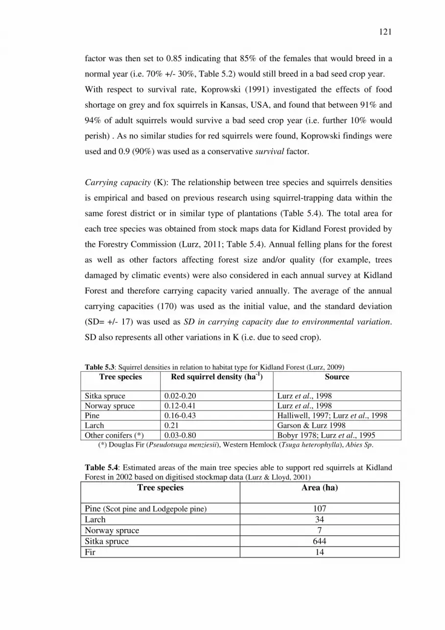
121
factor was then set to 0.85 indicating that 85% of the females that would breed in a
normal year (i.e. 70% +/- 30%, Table 5.2) would still breed in a bad seed crop year.
With respect to survival rate, Koprowski (1991) investigated the effects of food
shortage on grey and fox squirrels in Kansas, USA, and found that between 91% and
94% of adult squirrels would survive a bad seed crop year (i.e. further 10% would
perish) . As no similar studies for red squirrels were found, Koprowski findings were
used and 0.9 (90%) was used as a conservative survival factor.
Carrying capacity (K): The relationship between tree species and squirrels densities
is empirical and based on previous research using squirrel-trapping data within the
same forest district or in similar type of plantations (Table 5.4). The total area for
each tree species was obtained from stock maps data for Kidland Forest provided by
the Forestry Commission (Lurz, 2011; Table 5.4). Annual felling plans for the forest
as well as other factors affecting forest size and/or quality (for example, trees
damaged by climatic events) were also considered in each annual survey at Kidland
Forest and therefore carrying capacity varied annually. The average of the annual
carrying capacities (170) was used as the initial value, and the standard deviation
(SD= +/- 17) was used as SD in carrying capacity due to environmental variation.
SD also represents all other variations in K (i.e. due to seed crop).
Table 5.3: Squirrel densities in relation to habitat type for Kidland Forest (Lurz, 2009) Tree species
Red squirrel density (ha-1
) Source
Sitka spruce 0.02-0.20 Lurz et al., 1998
Norway spruce 0.12-0.41 Lurz et al., 1998
Pine 0.16-0.43 Halliwell, 1997; Lurz et al., 1998
Larch 0.21 Garson & Lurz 1998
Other conifers (*) 0.03-0.80 Bobyr 1978; Lurz et al., 1995 (*) Douglas Fir (Pseudotsuga menziesii), Western Hemlock (Tsuga heterophylla), Abies Sp.
Table 5.4: Estimated areas of the main tree species able to support red squirrels at Kidland
Forest in 2002 based on digitised stockmap data (Lurz & Lloyd, 2001)
Tree species
Area (ha)
Pine (Scot pine and Lodgepole pine) 107
Larch 34
Norway spruce 7
Sitka spruce 644
Fir 14

122
Initial population was set at 100 individuals, as that was the field-estimated number
of red squirrels in Kidland Forest in 2001, when the first survey was carried out.
Population was projected 11 years into the future (i.e. from 2001 to 2011) and
simulations were repeated 500 times (500 iterations).
5.2.2 Sensitivity analysis
Sensitivity analysis was carried out to assess how changes in carrying capacity (K)
were reflected in model outputs (i.e. number of squirrels).
Eleven K values arbitrarily selected were used to run the model. The scenario used as
baseline was the same scenario used for Kidland, and the model was run for 11 years.
The model outputs were recorded and plotted against carrying capacity values and
correlation was performed to visually and quantitatively assess model sensitivity.
5.2.3 Red squirrel population viability analysis at Abernethy Forest
Population viability analysis for red squirrels was carried out for Abernethy Forest
only as LiDAR data for this study area was of better quality (i.e. point density and
scan angle) and therefore habitat suitability maps were assumed to be more reliable
(see Chapter 3 and 4 for more details). Furthermore, and as opposed to Aberfoyle
Forest (the other study area) Abernethy is also one of the 18 proposed red squirrels
strongholds in Scotland.
5.2.3.1 Abernethy Forest
Abernethy Forest (57° 15’ N, 3° 40’ W) is owned and managed by the Royal Society
for the Protection of Birds (RSPB). Two thirds of the forest (19 km 2 ) is native forest
and one third is plantation. The dominant tree species is Scots pine (Pinus sylvestris
L). Detailed description of the forest and maps are provided in Chapter 2.
5.2.3.2 Model Input Data & Scenarios
In the case of Abernethy Forest, a gap area (see Figures 5.3 & 5.4) naturally divides
the study area into two distinctive zones and therefore two populations were
modelled. However, both populations are connected through patches of forest and the
gap was not considered to be large enough to prevent or reduce dispersal. Therefore,
dispersal among populations was modelled as 100%, as well as survival of
dispersers. Previous studies have shown that both red squirrel sexes disperse in the

123
same proportion (Wauters et. al., 2010) and therefore dispersal was modelled for
both males and females.
The rest of life-history data used to run the model for Abernethy Forest were the
same as used for Kidland Forest (see Table 5.3). Assumptions made are detailed in
section 5.2.1.3.
Catastrophe: Shortage of food was modelled as a catastrophe at Abernethy Forest
also. A study carried out by Summers & Proctors (2005) over an 11-year period
showed that Scots pine at Abernethy Forest produce a mast cone crop followed by a
poor cone crop every 3 years. Projections were made 20 years into the future, which
means that a poor cone crop could occur 6.5 times over that period. Thus, frequency
at which a cone crop failure may occur was set as 32 (i.e. a 32% probability of it
occurring any given year).
Severity of the catastrophe: The reaction of seed-eaters (including red squirrels) to
Scots pine cone crops patterns at Abernethy Forest was also investigated by
Summers (2011). He reports little to no noticeable change in number of cones taken
by squirrel in relation to cone production, suggesting little change in population size.
Based on this study and assuming that a small decrease in red squirrels reproduction
would still occur in a year with a poor cone production, a reproduction factor of 0.95
was used. As for Kidland Forest, Koprowski (1991) findings were used for
Abernethy Forest also and 0.9 (90%) was used as survival rate.
Carrying capacity (K)
Two different scenarios were modelled based on two different carrying capacities:
Basic and LiDAR.
Basic scenario: carrying capacity was calculated considering all the available mature
(i.e. old enough to produce food) forest. Carrying capacity was estimated as the
number of squirrels (per ha) that Scots pine support multiplied by the size of the area.
The mature forest (i.e. trees mature enough to produce food) area was estimated
based on available digital forest maps (ArcMap GIS; RSPB 2009, Figure 5.3).

124
LiDAR scenario: As part of this study, a GLM was developed that relates forest
structural parameters (i.e. canopy cover, number of trees and tree height) to the
number of cones stripped by squirrels (details provided in Chapter 2) . Using LiDAR
data, the GLM was extrapolated to the whole study area, and habitat suitability maps
were generated. These maps were classified into Low suitability (number of stripped
cones < 10) and Medium-to-High suitability (number of stripped cones �10; see
Chapter 4 for details). For the LiDAR scenario, those areas classified as Low
suitability were discarded for being of little or no use for squirrels (i.e. low canopy
cover, low tree density, trees not tall enough). Carrying capacity was then estimated
considering only Medium-to-High suitability patches on the LiDAR habitat
suitability maps (Figure 5.4).
Areas were calculated separately for each habitat type (i.e. All-forest and Medium-
to-High suitability) and for each population (Table 5.5).
Table 5.5: Area size and carrying capacity estimated for each population and habitat type, Abernethy
Forest, Scotland. Forest areas were extracted from digital stock maps provided by the RSPB (2009)
and Medium-to-high suitability patches are based on LiDAR habitat suitability maps.
Population 1 Population 2
All forest Medium to high
All forest Medium to high
Area (hectares) 395 162.6 366.5 104.6
Carrying capacity (number of squirrels)
328 135 304 87
Carrying capacity was then calculated (as described above) for each population.
Based on previous studies, the density of red squirrels per hectare for Scots pine in
Scotland is known to be between 0.33 and 0.83 in a poor and in a good cone crop
year respectively (Tittensor 1970; Moller, 1986; see also review by Lurz et al. 1995).
It was assumed that the first year of the period for which the model was run was a
good crop year and the higher value (i.e. 0.83) was used to calculate carrying
capacities.
Information on current red squirrel population size in Abernethy Forest is not
available and therefore Initial population was set as full carrying capacity (values
provided in Table 5.5) for both scenarios.
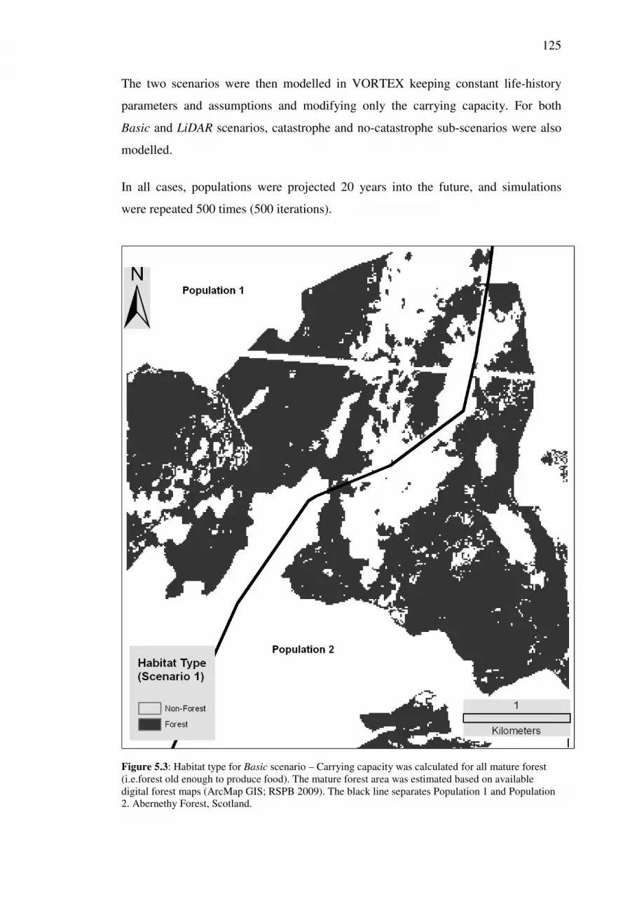
125
The two scenarios were then modelled in VORTEX keeping constant life-history
parameters and assumptions and modifying only the carrying capacity. For both
Basic and LiDAR scenarios, catastrophe and no-catastrophe sub-scenarios were also
modelled.
In all cases, populations were projected 20 years into the future, and simulations
were repeated 500 times (500 iterations).
Figure 5.3: Habitat type for Basic scenario – Carrying capacity was calculated for all mature forest
(i.e.forest old enough to produce food). The mature forest area was estimated based on available
digital forest maps (ArcMap GIS; RSPB 2009). The black line separates Population 1 and Population
2. Abernethy Forest, Scotland.

126
Figure 5.4: Habitat type for LiDAR scenario – based on LiDAR habitat suitability maps, Medium-to-
High suitability patches were retained. The black line separates Population 1 and Population 2.
Abernethy Forest, Scotland.

127
5.3 Results
5.3.1 Model Validation
Table 5.6 and Figure 5.5 show results of the model run for Kidland Forest. Annual
observed population ranges from 21 to 105, and annual mean predicted population by
VORTEX range from 72 to 110 individuals. Standard deviations of predictions are
also given in Table 5.6.
The number of squirrels estimated based on field observations was expected to be
within +/- 1SD of the VORTEX predicted populations. Whilst there was a mismatch
for early predictions (see Discussion) this was true for 7 out of 11 years (Figure 5.5).
Table 5.6: Numbers of squirrels observed in the field (Observed), mean number of squirrels
predicted by VORTEX (Projected) and standard deviation (SD)- Kidland Forest, UK
Population size 2001 2002 2003 2004 2005 2006 2007 2008 2009 2010 2011
Projected 110 104 101 97 90 87 84 80 76 74 72
Observed 100 21 26.5 28.5 21.5 36.5 74 104.5 45 112 44
SD (projected) 52.1 55.9 60.2 61.9 63.2 63.3 66.2 65.4 66 67.4 67.5
Figure 5.5: Plot of annual numbers of squirrels observed in the field (full line) and annual number of
squirrels predicted by VORTEX (dotted line) - Kielder Forest, UK
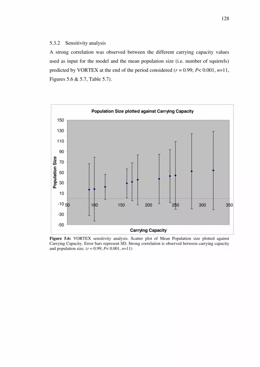
128
5.3.2 Sensitivity analysis
A strong correlation was observed between the different carrying capacity values
used as input for the model and the mean population size (i.e. number of squirrels)
predicted by VORTEX at the end of the period considered (r = 0.99; P< 0.001, n=11,
Figures 5.6 & 5.7, Table 5.7).
Population Size plotted against Carrying Capacity
-50
-30
-10
10
30
50
70
90
110
130
150
50 100 150 200 250 300 350
Carrying Capacity
Po
pu
lati
on
Siz
e
Figure 5.6: VORTEX sensitivity analysis. Scatter plot of Mean Population size plotted against
Carrying Capacity. Error bars represent SD. Strong correlation is observed between carrying capacity
and population size. (r = 0.99; P< 0.001, n=11)

129
Figure 5.7: Graph produced by VORTEX sensitivity test showing variation of Mean population size
with Carrying capacity. Values for K (1)….K(11) are given in Table 5.7
Table 5.7: Carrying capacity values used to perform the sensitivity analysis and mean annual
population predicted by VORTEX, Abernethy Forest, Scotland.
K (VORTEX)
Carrying Capacity
Mean Population
Size
SD
K(1) 90 17 49.6
K(2) 100 18 60.9
K(3) 120 22 24.1
K(4) 160 29 27.6
K(5) 170 32 36.2
K(6) 180 36 47.6
K(7) 220 38 47.3
K(8) 240 43 50.6
K(9) 250 44 64.5
K(10) 280 52 71.9
K(11) 320 53 75.0

130
5.3.3 Red squirrel population viability analysis at Abernethy Forest
In all scenarios and for both populations, mean population size showed a steady and
constant decline over the 20-year period (Figures 5.8 & 5.9). However, the
probability of extinction was much higher for the scenario based on LiDAR data,
indicating that management decision based on an overestimate of habitat suitability
(Basic scenario) can critically endanger local populations.
Basic scenario: For the no-catastrophe sub-scenario, mean population size decreased
from 260 to 42 for Population 1 and from 254 to 42 for Population 2. When one
catastrophe was modelled, mean population size decreased from 242 to 38 for
Population 1 and from 238 to 37 for Population 2. Considering both populations
together, probability of extinction at the end of the period was 53% and 58% for the
no-catastrophe and catastrophe sub-scenarios respectively.
LiDAR scenario: When no catastrophe was modelled, mean population size
decreased from 87 to 13 for Population 1 and from 78 to 11 for Population 2. For the
catastrophe scenario, mean population size decreases from 87 to 11 for Population 1
and from 76 to 9 for Population 2. Considering both populations together, probability
of extinction at the end of the period was 69% and 74% for the no-catastrophe and
catastrophe scenarios respectively.
Mean annual populations and standard deviations projected by VORTEX are
presented in Appendix D, Table D.1.

131
Figure 5.8: Annual population size for both Basic (full line) and LiDAR (dotted line) scenarios, for
Population 1 (top) and Population 2 (bottom), when no-catastrophe is modelled. Error bars represent
+/- SD. Abernethy Forest, Scotland.

132
Figure 5.9: Annual population size for both Basic (full line) and LiDAR (dotted line) scenarios, for
Population 1 (top) and Population 2 (bottom), when one catastrophe is modelled. Error bars represent
+/- SD. Abernethy Forest, Scotland.
133
5.4 Discussion
5.4.1 Model validation
One key criticism of PVA models is the simplification of population dynamics
Populations dynamics are complex and PVA provide only a relatively simple
estimation (Lindenmayer et al., 1993). In the particular case of VORTEX, population
dynamics are represented by the mean population size and variations (i.e.
fluctuations) in population size are represented by the standard deviation (Miller &
Lacy, 2005). Thus, VORTEX predictions were not expected to follow the natural
cycles of population dynamics. Instead, field estimated annual populations were
expected to be within the range of +/- the standard deviation of the annual mean
population projected by VORTEX. This was the case for 7 out of 11 years. The field
estimated population was considerably lower than that projected by VORTEX over
the 2002 to 2005 period (see Table 5.6 and Figure 5.5, Results section). In 2002,
most Scots pine plantations and some lodgepole pine plantations at Kidland Forest
were severely damaged by snow, and lost part or all of their crowns. This had a high
impact on the cone production and therefore on squirrel densities (Lurz, 2002).
However, the magnitude of this event and the extent of the spatial damage at Kidland
were not quantified during the survey. Hence, no data were available to accurately
model this catastrophe. Model predictions therefore overestimate the observed data
for the period 2002-2005. Once red squirrel population started to recover (in 2006),
field estimated population fall well within the range of +/- SD of model predictions.
PVA at Kidland Forest also illustrates the potential effects of environmental
stochasticity (i.e. snow event) on local populations. Furthermore, current model
predictions seem to indicate a reduction in mean predicted squirrel population at
Kidland Forest. Future field surveys will show if this is indeed the case, or a result of
input ranges for life history parameters which do not completely capture long term
population dynamics at Kidland Forest (see also 5.4.4).
5.4.2 Sensitivity analysis
Strong correlation (r=0.99, P < 0.001, n=11) between input values and model outputs
show that VORTEX is highly sensitive to variations in carrying capacity. In this
study, mainly variations in carrying capacity were modelled and the rest of the
parameters were kept constant. Therefore, only VORTEX’s sensitivity to carrying

134
capacity was tested. However, other researchers have found the model to be sensitive
to variations in a range of life-history parameters. For instance, Duca et al (2009)
found that variations in percentage of female breeding and adult mortality of white-
banded tanager in Brazil had an impact on probability of population persistence,
while the latter was not particularly sensitive to the percentage of males in the
breeding pool.
In addition, Brito & Grelle (2008) tested VORTEX’s sensitivity to mortality rate, sex
ratio, percentage of reproductive females and inbreeding depression for the Northern
muriqui, Brazil. Their findings showed that inbreeding depression, percentage of
female breeding and sex ratio influence population growth and final population size,
while variations in mortality rate produce variations in final population size. These
and the results from this Chapter suggest that VORTEX is in general fairly robust
and sensitive to variations in a range of parameters.
5.4.3 Red squirrel population viability analysis at Abernethy Forest
In general, and considering both scenarios, VORTEX predicts a steady reduction in
mean red squirrel population and a high probability of extinction (53%-58% for the
Basic scenario and 69%-74% for the LiDAR scenario, Figures 5.8 & 5.9). These
results match and support findings from a previous field study by Summers (2011)
who reports a decrease of the number of Scots pine cones taken by squirrels in
Abernethy Forest, and suggests a long-term decline in red squirrel population.
When carrying capacity is estimated using the LiDAR habitat suitability maps and
one catastrophe is modelled, the mean population at the end of the period reaches
very low numbers (11 for Population 1, 9 for Population 2) and a high probability of
extinction (74%). The difference in probability of extinction between catastrophe and
no-catastrophe scenarios is not large (55% and 53% respectively for the Basic
scenario, 74% and 69% for the LiDAR scenario). This was expected as the
percentage of females breeding was reduced by 5% only in a year when shortage of
food occurs (i.e. 95% of total females breeding will still breed in a bad cone crop
year). This conservative approach was based on research carried out by Summers
(2011), who reported no noticeable changes in red squirrel population -over an 11-
year period- in relation to food availability in Abernethy Forest. However, the reason
for this apparent lack of reaction of red squirrel could be that the species population
is already too small to react to peaks in food production. This could be indicating that

135
initial populations used to run VORTEX in this study (Table 5.5) are overestimating
the actual red squirrel population at Abernethy Forest, and the risk of extinction
could be even higher.
It should be highlighted here that PVA models provide probabilities and not
certainties (Brook et al, 1997; Boyce, 1992), as such, results should be cautiously
interpreted: for instance, high standard deviations for mean annual population sizes
(Table D.1, Appendix D) indicate a high uncertainty in predictions probably
stemming from high standard deviations in input life-history data (i.e. % of females
breeding, mortality rates, Table 5.2). Nevertheless, results of this study also suggest
that red squirrels populations are highly sensitive to variations in carrying capacity.
The high probability of extinction at the end of the 20-year period highlights the need
for forest management for the species conservation in Abernethy Forest, not only in
terms of habitat quality (i.e. increasing canopy cover and tree density) but also food
availability. In systems where more than one tree species is present, squirrels would
naturally switch to the tree species producing food (Andrén & Lemnell, 1992). This
is not possible in Abernethy Forest which consists of Scots pine only. Data from
Sweden show that in old-growth pine forests red squirrels may be naturally absent
for 2 out of 10 years as a result of cone crop cycles and changes in food availability
(Andrén & Lemnell, 1992). Data for Abernethy Forest (Summers, 2011) and this
study illustrate the potential constraints and challenges of single species management
in confined locations. Abernethy Forest is one of the oldest forests in Scotland and
part of the Scots pine woodlands are remnants of ancient native pine forests
(Summers, 2011). Therefore management options with respect to tree species
diversity to increase food availability for red squirrels need to be carefully
considered.
5.4.4 Issues and constrains
In both cases (i.e. Kidland and Abernethy Forests) VORTEX predicts a reduction in
mean squirrel population over time. The fact that this occurs in both Kidland and
Abernethy Forests could be indicating a feature of the model or life history parameter
ranges used that fail to sufficiently account for site specific events (Rushton et al.
2006b). It would therefore be interesting to contrast these results with empirical data
(i.e. field surveys and trap data giving details on population number, proportion of
animals breeding etc.), in particular for Kidland Forest where monitoring will

136
continue to be carried out on an annual basis (Lurz, pers. com; 2012). Furthermore,
some of the specific input parameter ranges (i.e. observed ecological data for
fecundity or mortality) used to run the model could also be having an effect on the
model predictions. Previous studies on red squirrel population dynamics found that
predicted population size for the Mt. Graham red squirrel in the United States was
sensitive to variations in parameters such as adult mortality, juvenile mortality,
fecundity and proportion of females breeding (Rushton et al.; 2006b); while in Italy,
the predicted total population size of grey squirrels were influenced by mean
fecundity and mean proportion of females with a first litter (Lurz et al., 2001).
In the current study, all parameters related to fecundity and mortality used to run the
model were gathered from published work on red squirrels in comparable forest
habitats. However, the use of site-specific data on red squirrel in for example
Kidland or Abernethy would certainly improve the accuracy and therefore the
reliability of the model predictions.
5.4.5 The use of LiDAR remote sensing for PVA
The main aim of this Chapter was .to assess the potential of LiDAR derived habitat
suitability data to assist red squirrels population viability analysis. Mills et al. (1996)
highlighted the importance of minimising the effects of projecting uncertainty
stemming from lack of accurate information in key parameters such as, for example,
carrying capacity when using PVA models. This study illustrates the risks of
overestimating habitat quality by, for example, not taking into consideration forest
structure. This overestimation of habitat quality and therefore, of carrying capacity
can lead to unrealistic projections and underestimate the actual risk of extinction of
local populations.
The use of LiDAR remote sensing in this context allows for a more refined
assessment of habitat quality by identifying patches that are of low suitability for the
species. This in turn allows for a more realistic estimation of carrying capacity. In
this way, this study also illustrates the potential of remote sensing, in particular
LiDAR, to produce more realistic estimates of carrying capacity, leading to more
realistic predictions of probability of extinction and population size when modelling
PVA for endangered species.
Abernethy Forest is one of the potential red squirrel strongholds in Scotland.
Management for strongholds at the stand level is contemplated in terms of conifer

137
species and age diversification to provide a continuous food supply
(http://www.scotland.gov.uk/Publications/2009/04/Red-Squirrel-Strongholds).
Habitat quality at the sub-stand level is not currently considered in management
plans, partly due to a lack of cost-efficient method to collect data and to generate
habitat quality information. The use of LiDAR remote sensing allows for the
identification of areas where forest structure management at the sub-stand level is
required. This is due to the capability of LiDAR to map habitat heterogeneity. In the
particular case of Abernethy, when habitat suitability is assessed considering the
species preferences in terms of forest structure and using LiDAR derived data,
approximately 70% of the forest (see Chapter 4) is not capable of sustaining red
squirrel populations in the long term. This highlights not only the need for
management for the forest, but also the advantages of using remote sensing to map
habitat quality at large scales.
To the author's knowledge, the current study represents one of the few that have used
remote sensing to assist PVA. One such study was carried out by Haines et al.
(2006). They incorporated remotely sensed data into a spatially-explicit package
(RAMAS/GIS) to model population viability for the endangered ocelot in USA.
Based on the species habitat preferences, habitat suitability data was incorporated to
the model as a land-cover map derived from LANDSAT ETM+ data where those
areas with canopy cover > 75% (identified by performing a supervised classification)
were (more details in Section 5.1.4.1) The current study illustrates the potential of
remote sensing as a tool to assist PVA modelling even when a no spatially-explicit
package such as VORTEX is used.
Overall, the results of this Chapter highlight the need for considering forest structure
when planning management for potential red squirrel reserves and the usefulness of
using LiDAR remote sensing to assess habitat quality at the forest scale.

138
CHAPTER 6
Discussion and conclusions
____________________________________________________________________
This thesis has addressed two critical gaps in red squirrel habitat management in the
UK. First, the study has investigated and quantified the relationship between red
squirrel habitat use and forest structural parameters, namely canopy closure, tree
density and canopy height. Second, the thesis has explored the use of remote sensing
–in particular LiDAR- to assist management of red squirrel habitat for the species
conservation. A population viability analysis was carried out to illustrate one of the
potential applications of LiDAR-derived habitat quality data. This chapter
summarises the findings of this research and discusses the limitations of the
approach. Further research needs and potential applications beyond the scope of this
study are also highlighted. Finally, overall conclusions and key recommendations are
provided.
6.1 Forest structure and red squirrel habitat preferences
This thesis investigated the effects of forest structure on red squirrel (Sciurus
vulgaris) habitat preferences. A general linear model (GLM) was used to relate red
squirrel feeding signs (as an indicator of local patch use; see Doumas & Koprowski
2012 for a similar approach) to forest structural parameters for Scots pine (Pinus
sylvestris). The statistical analysis of field-collected data showed that canopy closure
and number of trees are significant predictors (p < 0.01 and 0.03 respectively; n=52)
of the number of cones stripped by squirrels. Although strictly not significant (at the
0.05 significance level) tree height (p < 0.058) was retained as it is the only structural
variable considered in the model which is related to seed quality (Grönwall, 1982).
The statistical model (GLM) performance was assessed using a leave-one-out (LOO)
cross-validation approach (Arlot & Celisse, 2010). The correlation between field-
collected stripped cones and those predicted by the model was found to be moderate
(rs = 0.4, p <0.004, n=52, RMSE = 20). In ecological and biological field studies
variance in data is highly influenced by randomness and noise (i.e. outliers) and
therefore the levels of variance explained by statistical models are generally lower
139
than those in other sciences were experiments are carried out in controlled
environments (Møller, & Jennions, 2002). The three forest structural variables
considered in this study explained 43% of the variance in the number of cones
stripped by squirrels. This indicates that these are important factors that shape red
squirrel feeding behaviour at the sub-stand level.
The model developed in this study considered three forest structure parameters.
Other structural variables not considered in this study might also influence the
species habitat preferences at the plot level. Research by Nelson et al. (2005) found
that Delmarva fox squirrel (Sciurus niger cinereus ) prefer open understory in
Maryland’s Eastern Shore, USA. In the UK, Gurnell et al (2002) suggested that red
squirrel avoided open stands not only because of the open canopy, but also because
understory vegetation (in particular bracken) becomes denser in open stands making
it more difficult for the squirrels to move across quickly if needed. Future research
could explore the impact of understory vegetation in red squirrel habitat selection in
the UK.
Tree seeds are red squirrel main diet (Gurnell, 1987; Lurz et. al., 1995) and therefore
the question of whether squirrels would use more those plots where food is more
abundant, regardless the structure, has also been addressed in this thesis: the
relationship between total cone crop and number of stripped cones (per plot) was
assessed and results showed a weak to moderate correlation (rs=0.37, p<0.007; n=52,
Figure 6.1) between the total cone crop and the number of stripped cones per plot for
both Abernethy and Aberfoyle data together. If the presence and abundance of food
explained habitat use by red squirrel at the plot level, a much stronger correlation
would be expected.
In addition to this, and using the data from the survey that has been carried out at
Kidland Forest for the last 11 years (2001 to 2011; Lurz, 2011) the relationship
between mean annual mean cone density and red squirrel density for the whole forest
and considering all tree species together was also assessed. In this case, and as
observed by Lurz (2011), a much stronger correlation was found (rs=0.87, p<0.001;
n=11).
These results suggest that while annual variations in food availability shape the
number of red squirrels at the forest level, at the sub-stand level, and provided food is

140
available, forest structure matters and has an impact on habitat selection by red
squirrels.
The current study is based on 2 years of fieldwork and further research is required to
test the robustness of the predictions. For example, whilst squirrels were seen to
avoid open areas that contain food, it is unknown what would happen in times of
food shortage, and what risks they would be prepared to take. Furthermore, in times
of scarce resources, subordinate individuals in a population (i.e. sub-adults and
juveniles) have limited access to those resources (i.e. food), which would also be the
case if high densities of squirrels occur (Gurnell, 1987). It would be interested to
explore if squirrels would exploit isolated stands or open forest in those situations.
Whilst this investigation of squirrel habitat use based on feeding signs represents a
first and relatively crude approach, the findings confirm previous research by Gurnell
et al (2002). The latter reported that red squirrels in Thetford Forest were observed to
avoid old stands of Scots pine (Pinus sylvestris) that had been intensively thinned
(i.e. few trees and open canopy). This thesis, however, goes one important step
further by quantifying the effect of forest structure on red squirrel habitat use.

141
Figure 6.1: Scatter plot of number of stripped cones and total cone crop per plot for Scots pine
(rs=0.37, P<0.007; n=52). Abernethy and Aberfoyle Forest, Scotland
Figure 6.2: Scatter plot of field estimated red squirrel population and mean cone density (m
2) for all
tree species together – annual values (rs=0.87, P<0.001; n=11). Kidland Forest, England.
142
6.2 The use of LiDAR remote sensing
In this thesis, LiDAR remote sensing was used to i) retrieve forest structural
parameters that relate to red squirrel habitat use, more specifically, the three
variables discussed in the previous section: canopy cover (as a surrogate for canopy
closure, see Chapter 3), number of trees and tree height; and ii) to map habitat
suitability over the whole study areas using the LiDAR derived variables and the
GLM.
Forest structural parameters
The statistical analysis of the relationship between forest structure and red squirrel
habitat use focused on Scots pine. However, data on forest structure was also
collected for sitka spruce (Picea sitchensis) at Aberfoyle. Field collected data for
both tree species were used to validate LiDAR derived explanatory variables, and in
both cases (i.e. field and LiDAR data), mean values at the plot level were used. A
summary of the main findings is provided below:
Field-measured canopy closure and LiDAR-derived canopy cover were found to be
strongly correlated when all Scots pine plots were considered together (rs= 0.71;
n=52, P< 0.00). Large LiDAR scan angles (i.e. > 18°) are thought to produce slightly
biased canopy cover estimates (Korhonen et al., 2011). Scan angles for Abernethy
and Aberfoyle LiDAR data were 18° and 20° respectively and therefore, correlations
were also assessed for Scots pine at each forest separately with similar results (rs=
0.65 & 0.73; n=32 & 20, p<0.00 for Abernethy and Aberfoyle respectively). These
results are not conclusive and only suggest that no substantial differences were
observed between canopy cover derived from LiDAR data acquired at scan angles of
18° and 20°. However, the optimal scan angle is 12° and a maximum of 15° is
recommended to avoid bias in the estimation of forest structural parameters (Evans et
al., 2009). The results of this thesis suggest that strong correlations between LiDAR
canopy cover and field canopy closure are observed with scan angles larger than those
recommended for vegetation applications. Nevertheless, future research should explore
the correlation between canopy cover and canopy closure using LiDAR data acquired at
scan angles <15°.

143
The correlation between canopy cover and canopy closure was assessed also for sitka
spruce plots only and was found to be weaker (rs=0.40, p< 0.015, n=36). As the key
tree species in this project is Scots pine, this was not further investigated. However,
tree species can differ significantly with respect to crown structure as illustrated by
Scots pine and sitka spruce. If the approach is intended to be applied to other tree
species or mixed woodlands, the relationship between canopy closure and canopy
cover needs to be carefully explored in each case.
Local maxima algorithm provides an operational approach to retrieve the number of
trees using LiDAR data. The level of accuracy achieved in Abernethy Forest (71,1%,
LiDAR data resolution: 2 pulses/m2) lies within the range of values found in the
literature (e.g Gaulton et al, 2008; García et. al., 2007). However, the percentage of
trees correctly detected in Aberfoyle is considerably lower (47.7%). The main reason
for this is likely to be the lower LiDAR data resolution (1 pulses/m2). Higher point
densities (i.e. >1 pulses/m2) would potentially improve the number of detected trees
(this is further discussed later in this section). The performance of local maxima is
also likely to improve if a variable-size search window is used, as opposed to the
fixed-size window that was used in this study. Provided that reliable allometric
relationships are available, search-window size could be a function of the tree height
(this has been discussed in more detail in Chapter 3). Finally, the use of a different
approach or a combination of techniques (e.g. local maxima and image segmentation,
see Chapter 3) might also produce more accurate results.
Accurate mean tree height at the plot level can be estimated by using 95th
percentile
of LiDAR height. This correlation was investigated for plots consisting of Scots pine
only at Abernethy and for both Scots pine and sitka spruce plots together at
Aberfoyle. Results were very similar in both cases (r=0.92 and 0.94; n= 32 and 56
respectively, P< 0.001) suggesting that 95th
percentile of LiDAR height accurately
represents mean tree height at the plot level for those three species. Future research
could investigate the use of LiDAR percentiles for different types of forest; e.g. even
aged plantations and natural mixtures with a variety of ages and species.

144
GLM implementation
The LiDAR derived explanatory variables were used to implement the general linear
model and map habitat suitability in both Abernethy and Aberfoyle Forests (Chapter
4). As the GLM was originally developed for Scots pine only, in Aberfoyle, only
Scots pine stands were used to implement the model. LiDAR performance was
assessed by exploring the correlation between field-predicted and LiDAR-predicted
number of stripped cones. Correlations were assessed for each study area separately
and were found to be strong (rs = 0.59 for Abernethy and rs = 0.54 for Aberfoyle, n=
32 and 20; RMSE= 12.3 and 11.9 respectively). Assuming the number of stripped
cones as an index of habitat selection by red squirrels, these strong correlations
highlight the usefulness of LiDAR as a tool to assist red squirrel habitat management
at large-scale.
The recommended pulse density for vegetation applications is 4-6 pulses/m2 (Evans
et al, 2009). The current study suggests that accurate results can still be achieved
using lower point densities (1 and 2 pulses/m2
for Aberfoyle and Abernethy
respectively). However, this study also illustrates some of the potential constraints.
The number of trees is the parameter where the effect of low pulse density seems
more evident, in particular for Aberfoyle. This was expected to have an effect on the
performance of the LiDAR-based model predictions. In order to quantitatively assess
this effect, the Aberfoyle LiDAR number of trees was calibrated using field data (see
Chapter 4) and the GLM was also implemented using the calibrated LiDAR number
of trees. This correction improved the model performance (rs = 0.60) but it also
increased the error (RMSE = 29.8). This suggests that while this calibration improves
the spatial variation of LiDAR-derived number of stripped cones it also increases the
difference between absolute values of field-predicted and LiDAR-predicted number
of stripped cones. While these results are not conclusive in terms of the actual
accuracy of the model, they do reflect that the poor performance of the LiDAR
derived number of trees influences the accuracy of the habitat suitability maps. As
this poor performance is likely to be caused by the low pulse density, this highlights
the need for using higher resolution LiDAR data to assess and monitor habitat
suitability for red squirrel. However, increasing point density (and decreasing scan
angle as suggested above) also increases acquisition cost and data volume (Evans et
al., 2009). Since LiDAR data can be used for multiple applications (i.e. forest

145
inventories, topography mapping) establishing collaborative projects to share data
could potentially reduce the cost of data acquisition and processing.
This project aimed to assess the ecological relationship between red squirrel habitat
use and forest structure, and therefore, this part of the project was developed first
using data collected in the field. LiDAR data were used afterwards to extrapolate the
analysis to both study areas by using LiDAR-derived explanatory variables which
replaced the field-measured explanatory variables. Most studies have used a different
approach by directly exploring the relationship between species presence/abundance
(or habitat use) and LiDAR derived metrics (see. Hill et. al., 2005; Clawges et.
al.,2008; Goetz et. al.,2010 for examples). Future research could explore the
applicability of the latter to the red squirrel in the UK. For instance, using squirrel
survey techniques such as radio-tracking or camera-trap would provide information
on specific patch use. Integrating this information and LiDAR derived metrics into a
GIS would allow a better understanding of how three-dimensional forest
characteristics (such as canopy height, canopy cover, tree density) shape squirrels
space use and impact on aspects of for example population dynamics (and predation
rates) or red-grey squirrel competition.
A synergetic approach using optical and LiDAR remote sensing could provide the
opportunity to map not only forest structure (LiDAR) but also other aspects of red
squirrel habitat preferences. Most studies carried out in the UK investigating the
species habitat preferences have used forest stock maps (e.g. Lurz et al, 1995;
Gurnell et al, 2002) or the National Inventory of Woodlands and Trees (NIWT, e.g.
Poulsom et al., 2003) to assess tree species composition. However, forests and
woodlands can change over the years and forest stock maps have been found to be
outdated in a number of occasions (Jo Ellis, personal Comm., 2009; author’s
personal observation). Updating this information is time consuming and requires
extensive field surveys. For instance, the current National Forest Inventory began in
2009 and it is expected to be completed in 2014 (Forestry Commission, 2012).
A number of studies have used remote sensing to map forest species composition
with reasonable levels of accuracy: Martin et. al., (1998) used AVIRIS hyperspectral
data (224 contiguous spectral bands ranging from 0.4 to 2.4 µm; 20m spatial
resolution) to generate tree species maps of pure and mixed stands of conifer and

146
deciduous forests in Massachusetts, US; with an overall accuracy of 75%; while
Lucas et. al. (2006) used CASI data (14 spectral bands, 1 m spatial resolution) to
accurately (70%) classify tree species composition in a natural forest in Australia.
From a “remote sensing” point of view, northern hemisphere forests have the
advantage of having a relatively simple species composition, which facilitates the
discrimination and mapping of tree species (Lucas et. al. 2008). In the UK, a study
by Hill et al (2010) reported a maximum overall accuracy of 82% when using time-
series multispectral data (ATM, 11 spectral bands) to classify tree species at Monks
Wood, an ancient semi-natural deciduous forest.
The above examples illustrate the potential of remote sensing to provide additional
information to assist red squirrel habitat management. The combination of both
forest structure and species composition derived from remote sensing data could
substantially improve habitat assessment for red squirrel in the UK by providing
accurate information on a range of habitat requirements that would be prohibitively
expensive and time consuming to gather in the field. Furthermore, mapping species
composition using remote sensing could also provide a tool to regularly update forest
stock maps and forest inventories.
Habitat suitability and population viability analysis (PVA)
Habitat suitability maps were created for both study areas. Out of the total forest
area, 27% at Abernethy Forest and 37% at Aberfoyle (considering only the un-
calibrated number of trees) were classified as Medium-to-High suitability (Chapter
4). Assuming that only Medium-to-High suitability patches can support resident
populations of squirrels in the long-term, this means that only approximately one
third of the forests is actually suitable for the species. This is one of the key findings
of this thesis and has implications for the conservation of the species, in particular in
Abernethy Forest, which is one of the proposed red squirrel strongholds.
To i) illustrate one of the potential applications of LiDAR derived habitat suitability
information and ii) assess the impact of forest structure on the long-term survival of
the species, a PVA was carried out. Carrying capacity was calculated based on the
LiDAR-derived habitat suitability data, and the viability and risk of extinction of the
species populations at Abernethy Forest were estimated. In general, and for all
modelled scenarios (Chapter 5), results of the PVA suggested a reduction in red

147
squirrel population. It is not clear if this is indeed the case, or if the model
predictions are influenced by input ranges in life history parameters which do not
completely capture long term population dynamics at Abernethy Forest. However,
these results support previous research by Summers (2011) who suggested a long-
term decline in red squirrel population in the forest.
Being a mono-species forest, Abernethy is a good example of the constraints and
challenges of single species management in confined locations. It would be
interesting to model different scenarios, including diversification and changes in the
proportions of different tree species to evaluate management options.
When LiDAR derived habitat quality data was used to estimate carrying capacity,
results suggest a high risk of extinction (74%) for the species populations in 20 years
and very low densities (approximately 10 individuals in each of the two populations
modelled). While results from PVA need careful interpretation due to the high levels
of uncertainty typically associated with these types of models, these results highlight
the need for considering forest structure when managing forests for red squirrel
conservation and the usefulness of LiDAR remote sensing to assist this management.
Further research could integrate LiDAR derived suitability maps into spatially-
explicit PVA models (e.g. RAMAS/GIS) to model more complex spatial-scenarios
such as the viability and potential dispersal of red squirrel meta-populations based on
the size and habitat quality of different patches in a forest. Furthermore, if grey
squirrel habitat preferences in terms of structure were known, potential risk-of-
competition maps could be derived from LiDAR data and red squirrel population
viability could be modelled by manipulating, for instance, reproduction rates
(Gurnell et. al. 2004) to account for the competition with the greys. A similar
approach could be used to assess the effects of predation on the viability of red
squirrel populations by modelling, for example, different mortality scenarios.
6.3 Transferability, repeatability and further applications of methods
The data collection methodology used in this project can be only used in conifer
forests as it relies on the presence of feeding remains (stripped conifer cones) to
assess and quantify habitat use by red squirrel. The GLM was developed using data
from two different study areas but focused on the same tree species (i.e. Scots pine).

148
Further research could aim to test the transferability of this methodology to more
complex, heterogeneous conifer ecosystems.
The implementation of the GLM using LiDAR-derived explanatory variables proved
transferable between the two study sites. The results were influenced by acquisition
parameters such as LiDAR pulse density and potentially scan angle. Higher pulse
densities are likely to improve the accuracy of LiDAR-derived variables and
therefore, of the habitat quality data.
The methodology developed in this thesis can assist current management and future
monitoring of strongholds to ensure that these reserves meet the species
requirements.
The red squirrel is being replaced by the greys not only in the UK but also in other
European countries such as Ireland, Italy and Switzerland (Lurz et al, 1995; Rushton
et al, 2000; Gurnell et. al., 2004; Teangana et al., 2000). The methodology
developed in this thesis can be applied to the same species in other countries.
The transferability of the LiDAR-based methodology to tree species other than Scots
pine (and potentially sitka spruce) was not assessed in this thesis. If the approach is
intended to be applied to other conifer species, mixed woodlands or deciduous
forests, validation using field data would need to be performed in order to assess the
extent to which LiDAR-metrics can be used as estimators of ground data.
6.4 Contribution of research
It had been previously suggested that red squirrels would avoid open stands (Gurnell
et al., 2002), however this had not been statistically analysed and quantified. This
thesis has moved one step forward and has quantified the relationship between forest
structure parameters such as canopy closure, tree density and tree height and red
squirrel habitat use for Scots pine in the UK.
This thesis has also developed a methodology to assess habitat suitability for red
squirrel over large areas by using LiDAR remote sensing. This methodology
produces accurate results without demanding extensive field work, although –as in
any remote sensing-based approach- field data needs to be collected to assess the
accuracy of LiDAR derived data. This study also explores the potential of LiDAR
derived number of trees as an input to assess red squirrels habitat quality.

149
When considered together, the quantification of the relationship between forest
structure and habitat use by red squirrels, and the development of a methodology to
implement the analysis over a large area, these findings allow for a more refined and
integral assessment of habitat suitability at the sub-stand level considering not only
food availability but also other factors such as the provision of shelter and reduced
risk of predation. This study also represents the first to integrate remote sensing into
habitat mapping for red squirrel in the UK.
Although PVA have been widely used to assess management strategies for
endangered species conservation, few previous studies have incorporated information
derived from remote sensing to assist species management. This thesis illustrates the
potential of LiDAR derived data to assist PVA within a non-spatially explicit model
as VORTEX by, for example, providing more accurate estimates of carrying
capacity.
Finally, this study has contributed to address the challenge of multidisciplinary work
involving the integration of ecology and remote sensing to map habitat and assist
management for endangered species over large areas.
6.5 Overall conclusions
- Forest structure parameters, namely canopy closure, tree density and tree
height, influence red squirrel habitat use at the sub-stand level for Scots pine.
Further research is needed to test the robustness of the approach and its
transferability to more complex mixed conifer forests
- Airborne LiDAR data can be used to assess habitat quality for red squirrel.
Higher densities point data and smaller scan angles than those used in this
study could potentially improve the effectiveness of the approach.
- Habitat quality for one of the 18 proposed strongholds (Abernethy Forest)
was assessed and results showed that at present, less than one third of the
forest is actually suitable for the species. Considering that these strongholds
could potentially become the only hope for the species survival in the UK,
this is one of the key findings of this thesis.

150
6.6 Key recommendations
From both previous research on red squirrel habitat preferences and the current
study, managing forests for the species should considered the following:
1- Conifer forests > 2000 ha (Lurz et al., 1995; Pepper & Patterson, 2001;
Gurnell et al., 2002; Bryce et al., 2005)
2- Avoidance of large seeded broadleaves (i.e. oak, chestnut, beech and
hazel; Lurz et al., 1995; Bryce et al., 2005; )
3- Mixture of conifer species and age structure to ensure food supply (Lurz
et al., 1995; Gurnell et al., 2002; Bryce et al., 2005)
1- Management for red squirrel also needs to contemplate the preference of
the species for dense canopies (Flaherty et al.; 2012)
In terms of LiDAR data, key recommendations are:
1- LiDAR data point densities � 2 pulses/m2
2- LiDAR scan angles � 15°
3- Collaborative data-sharing partnerships to reduce costs of data acquisition
and processing

151
EPILOGUE
To a Squirrel at Kyle-na-gno
COME play with me;
Why should you run
Through the shaking tree
As though I’d a gun
To strike you dead?
When all I would do
Is to scratch your head
And let you go.
W.B. Yeats; The Wild Swans at Coole, 1919

152
REFERENCES
Abileah, R. 2001. Use of high resolution space imagery to monitor the abundance,
distribution, and migration patterns of marine mammal populations. OCEANS
3: 1381-1387.
Agresti, A. 2002. Categorical data analysis, New York, Wiley-Interscience.
Ahokas, E., Yu, X., Oksanen, J., Hyyppä, J., Kaartinen, H. and Hyyppä, H. 2005.
Optimization of the scanning angle for countrywide laser scanning. In
Proceeedings of the International Archives of Photogrammetry, Remote
Sensing and Spatial Information Sciences, G. Vosselman and C. Brenner
(Eds). XXXVI, Part 3/W19, 115-119.
Andrén H. and Lemnell P. 1992, Population Fluctuations and Habitat Selection in the
Eurasian Red Squirrel Sciurus vulgaris. Ecography 15: 303-307.
Arlot, S. and Celisse, A. 2010. A survey of cross-validation procedures for model
selection. Statistics Surveys 4: 40-79.
Atkin, J.W., Radford, A.D., Coyne, K.P., Stavisky, J. and Chantrey, J. 2010.
Detection of squirrel poxvirus by nested and real-time PCR from red (Sciurus
vulgaris) and grey (Sciurus carolinensis) squirrels BMC Veterinary Research
6.
Baltsavias, E.P. 1999. Airborne laser scanning: basic relations and formulas. Isprs
Journal of Photogrammetry and Remote Sensing 54: 199-214.
Begon, M., Harper, J. and Townsend, C. 1996, Ecology: Individuals, populations
and communities, Blackwell Science, Oxford.
Bobyr, G.Y. 1978. A contribution to the ecology of the Altaian squirrel (Sciurus
vulgaris altaicus) acclimatized. Zoologichesky Zhurnal 57: 253-259.
Bosch, S. & Lurz, P.W.W. 2012. The Eurasian Red Squirrel Sciurus vulgaris (First
edition) Westarp Wissenschaften, Hohenwarsleben, Germany
Boyce, M. 1992. Population viability analysis. Annual Review of Ecology and
Systematics 23: 481-506.
Bradbury, R., Hill, R., Mason, D.C., Hinsley, S.A., Wilson, J.D., Baltzer, H.,
Anderson, G.Q.A., Whittingham, M.J., Davenport, I.J. and Bellamy, P.E.
2005. Modelling relationships between birds and vegetation structure using
airborne LiDAR data: a review with case studies from agricultural and
woodland environments. British Ornithologists' Union, Ibis 147: 443-452.
Brito, D. and Grelle, C.E.V. 2006. Estimating minimum area of suitable habitat and
viable population size for the northern muriqui (Brachyteles hypoxanthus),
Biodiversity and Conservation 15: 4197-4210.
Broome, A., Hendry, S. and Peace, A. 2007. Annual and spatial variation in coning
shown by the Forest Condition Monitoring programme data for Norway
spruce, sitka spruce and Scots pine in Britain, Forestry 80: 17-28.
Brook, B.W., Lim, L., Harden, R., & Frankham, R. 1997. Does population viability
analysis software predict the behaviour of real populations? A retrospective
study on the Lord Howe Island woodhen Tricholimnas sylvestris (Sclater).
Biological Conservation, 82: 119-128
Brook, B.W., Cannon, J.R., Lacy, R., Mirande, C. and Frankham, R. 1999.
Comparison of the population viability analysis packages GAPPS, INMAT,
RAMAS and VORTEX for the whooping crane (Grus americana), Animal
Conservation 2: 23-31
153
Brook, B.W., O'Grady, J.J., Chapman, A.P., Burgman, M.A., Akcakaya, H.R., &
Frankham, R. 2000. Predictive accuracy of population viability analysis in
conservation biology. Nature, 404: 385-387
Brovelli, M.A., Cannata, M. and Longoni, U.M. 2002. Managing and processing
LIDAR data within GRASS. Proceedings of the Open source GIS - GRASS
users conference 2002, 1-29.
Burgman, M. and Possingham, H.P. 2000. Population viability analysis for
conservation: the good, the bad and the undescribed. Pages 97-112 in:
Genetics, Demography and Viability of Fragmented Populations. Eds Young,
A.G & Clarke, G.M. Cambridge University Press, London
Burgman, M., Franklin, J., Hayes, K.R., Hosack, G.R., Peters, G.W., & Sisson, S.A.
2012. Modeling Extreme Risks in Ecology. Risk Analysis 32: 1956-1966
Bruemmer, C.M., Rushton, S.P., Gurnell, J., Lurz, P.W.W., Nettleton, P., Sainsbury,
A.W., Duff, J.P., Gilray, J. and McInnes, C.J. 2010. Epidemiology of
squirrelpox virus in grey squirrels in the UK. Epidemiology and Infection 138:
941-950.
Bryce, J., Cartmel, S. and Quine, C.P. 2005. Habitat use by red and grey squirrels:
results of two recent studies and implications for management, Forestry
Commission Information Note No. 76.
Carrascal, L.M. and Telleria, J.L. 1988. Relationships among birds and vegetation
structure in the agricultural landscape of the atlantic basque country. Ciencias
Naturales 40: 9-17.
Clawges, R., Vierling, K., Vierling, L. and Rowell, E. 2008. The use of airborne
LiDAR to assess avian species diversity, density, and occurrence in a
pine/aspen forest. Remote Sensing of Environment 112: 2064-2073.
Cook, J.G., Stutzman, T.W., Bowers, C.W., Brenner, K.A. and Irwin, L.L. 1995.
Spherical densiometers produce biased estimates of forest canopy cover.
Wildlife Society Bulletin 23: 711-717.
Crawley, M. 2007. The R Book. Chichester, England. John Wiley & Sons Ltd.
De Lamo, X. 2010. Mapping red squirrel (Sciurus vulgaris) habitat suitability using
GIS and remote sensing techniques Edinburgh, UK University of Edinburgh,
MSc.
Doak, D.F., Finkelstein, M.E. and Bakker, V.J. 2009. Population Viability Analysis,
in Levin, S.A. (Eds) The Princeton Guide to Ecology, Princeton University
Press, Princeton, 521-528.
Doo-Ahn Kwak, Woo-Kyun Lee, Jun-Hak Lee, Greg S. Biging, Peng Gong. 2007.
Detection of individual trees and estimation of tree height using LiDAR data.
Journal of Forest Research 12: 425-434
Doumas, S. & Koprowski1, J.L.; 2012, Return of Fire as a Restoration Tool: Long-
Term Effects of Burn Severity on Habitat Use by Mexican Fox Squirrels,
Restoration Ecology, DOI: 10.1111/j.1526-100X.2012.00864.x
Duca, C., Yokomizo, H., Marini, M.A., & Possingham, H.P. 2009. Cost-efficient
conservation for the white-banded tanager (Neothraupis fasciata) in the
Cerrado, central Brazil. Biological Conservation, 142: 563-574
Edelman, J., Koprowski, J.L. and Bertelsen, S.R. 2009. Potential for nest site
competition between native and exotic tree squirrels. Journal of Mammalogy
90: 167-174.
Ene, L., Naesset, E. and Gobakken, T. 2012. Single tree detection in heterogeneous
boreal forests using airborne laser scanning and area-based stem number
estimates. International Journal of Remote Sensing 33: 5171-5193.

154
Evans, J.S., Hudak, A.T., Faux, R. and Smith, A.M.S. 2009. Discrete Return Lidar in
Natural Resources: Recommendations for Project Planning, Data Processing,
and Deliverables, Remote Sensing 1: 776-794.
Faraway, J.J. 2005. Linear models with R. Boca Raton, Florida, Chapman &
Hall/CRC.
Faraway, J.J. 2006. Extending the linear model with R. Boca Raton, Florida,
Chapman & Hall/CRC.
Fiegna, C. 2011. A study of squirrelpox virus in red and grey squirrels and an
investigation of possible routes of transmission, Edinburgh, UK, University of
Edinburgh, PhD.
Flaherty, S., Patenaude, G., Close A. and Lurz, P. 2012. The impact of forest-stand
structure on red squirrel habitat use, Forestry: An International Journal of
Forest Research, doi:10.1093/forestry/cps042.
Forestry Commission UK. 2006. The Scottish forestry strategy.
http://www.forestry.gov.uk/sfs accessed 2012
Forestry Commission UK. 2009. Red squirrel strongholds consultation,
http://www.forestry.gov.uk/ accessed 2012
Forestry Commission UK, 2012, http://www.forestry.gov.uk/inventory, accessed
2012
Garcia, C. 2006. Locating potential red squirrel (Sciurus vulgaris) habitat in Kielder
Forest, Northumberland with Quickbird imagery and object-oriented
classification Edinburgh, UK University of Edinburgh, MSc.
García, R., Suárez, J.C. and Patenaude, G. 2007. Delineation of individual tree
crowns for LiDAR tree and stand parameter estimation in Scottish woodlands.
Lecture Notes in Geoinformation and Cartography Part 2, 55-85.
Gaulton, R. 2008. Remote sensing for continuous cover forestry: quantifying spatial
structure and canopy gap distribution. School of Geosciences. Edinburgh,
Edinburgh, PhD
Gaulton, R., & Malthus, T.J. 2010. LiDAR mapping of canopy gaps in continuous
cover forests: A comparison of canopy height model and point cloud based
techniques. International Journal of Remote Sensing 31: 1193-1211
Gerber, L. & González-Suárez, M. 2010. Population Viability Analysis: Origins and
Contributions. Nature Education Knowledge, 1(11):15
Goetz S.J., Steinberg D., Betts M.G., Holmes R.T., Doran P.J., Dubayah R. and
Hofton M. 2010. Lidar remote sensing variables predict breeding habitat of a
Neotropical migrant bird. Ecology 91: 1569-1576.
Graf, R.F., Mathys, L. and Bollmann, K. 2009. Habitat assessment for forest
dwelling species using LiDAR remote sensing: Capercaillie in the Alps.
Forest Ecology and Management 257: 160-167.
Grönwall, O. 1982. Aspects of the food for red squirrels (Sciurus vulgaris L.).
Stockholm, Sweden.University of Stockholm. PhD: pp.131.
Gougeon, F.A., 1995. A crown-following approach to the automatic delineation of
individual tree crown in high spatial resolution aerial images, Canadian
Journal of Remote Sensing, 21(3):274–284.
Gougeon, F.A. and Leckie, D.G. 2006. The Individual Tree Crown Approach
Applied to Ikonos Images of a Coniferous Plantation Area. Photogrammetric
Engineering & Remote Sensing 72: 1287–1297.
Gurnell, J. 1983. Squirrel numbers and the abundance of tree seeds. Mammal Review
13: 133-148.
Gurnell, J. 1987. The natural history of squirrels. Christopher Helm, London.

155
Gurnell, J. and Pepper, H.W. 1991. Conserving the Red Squirrel. Forestry
Commission Research Information Note 205, HMSO, London.
Gurnell, J. and Pepper, H.W. 1993. A critical look at conserving the British Red
Squirrel Sciurus vulgaris. Mammal Review 23: 127-137.
Gurnell, J., Clark, M.J., Lurz, P.W.W., Shirley, M.D.F. and Rushton, S.P. 2002.
Conserving red squirrels (Sciurus vulgaris): mapping and forecasting habitat
suitability using a Geographic Information System Approach. Biological
Conservation 105: 53-64.
Gurnell, J., Wauters, L.A., Lurz, P.W.W. and Tosi, G. 2004, Alien species and
interspecific competition: effects of introduced eastern grey squirrels on red
squirrel population dynamics. Journal of Animal Ecology 73: 26-35.
Gurnell, J., Lurz, P.W.W., McDonald, R. and Pepper, H. 2009. Practical techniques
for surveying and monitoring squirrels. Forestry Commission Practice Note
11, pp. 1-12, FC Alice Holt Lodge, Farnham, Surrey, UK.
Guo, J., Chen, Y. and Hu, J. 2002. Population viability analysis of giant pandas in the
Yele Nature Reserve. Nature Conservation, 10: 35-40.
Haines, A.M., Tewes, M.E., Laack, L.L., Horne, J.S. and Young, J.H. 2006. A
habitat-based population viability analysis for ocelots (Leopardus pardalis) in
the United States. Biological Conservation 132: 424-436.
Halliwell, E.C. 1997. Red squirrel predation by Pine martens in Scotland. The
Conservation of Red Squirrels, Sciurus vulgaris L. (Eds J. Gurnell and
P.W.W. Lurz), pp.39-48 Peoples Trust for Endangered Species, London.
Hamby, D.M. 1995. A comparison of sensitivity analysis techniques, Health physics
68: 195-204.
Heblinski, J., Schmieder, K., Heege, T., Agyemang, T.K., Sayadyan, H. and
Vardanyan, L. 2011. High-resolution satellite remote sensing of littoral
vegetation of Lake Sevan (Armenia) as a basis for monitoring and assessment.
Hydrobiologia 661: 97-111.
Hill, R.A., Hinsley, S.A., Gaveau, D.L.A. and Bellamy, P.E. 2004. Predicting habitat
quality for Great Tits (Parus major) with airborne laser scanning data.
International Journal of Remote Sensing 25: 4851-4855.
Hill, R.A., Wilson, A.K., George, M., and Hinsley, S.A. 2010. Mapping tree species
in temperate deciduous woodland using time-series multi-spectral data.
Applied Vegetation Science 13: 86-99
Holmgren, J. 2004. Prediction of tree height, basal area and stem volume in forest
stands using airborne laser scanning. Scandinavian Journal of Forest
Research 19: 543-553.
Hopkinson, C., Chasmer, L. and Hall, R.J. 2008. The uncertainty in conifer
plantation growth prediction from multi-temporal lidar datasets. Remote
Sensing of Environment 112: 1168-1180.
Hyde, P., Dubayah, R., Peterson, B., Blair, J.B., Hofton, M., Hunsaker, C., Knox, R.
and Walker, W. 2005. Mapping forest structure for wildlife habitat analysis
using waveform lidar: Validation of montane ecosystems. Remote Sensing of
Environment 96: 427-437.
Hyyppa, J., Kelle, O., Lehikoinen, M. and Inkinen, M. 2001. A segmentation-based
method to retrieve stem volume estimates from 3-D tree height models
produced by laser scanners. IEEE Trans. Geosci. Remote Sensing 39: 969-
975.
Hyyppa, J., Hyyppa, H., Leckie, D., Gougeon, F., Yu, X. and Maltamo, M. 2008.
Review of methods of small-footprint airborne laser scanning for extracting
156
forest inventory data in boreal forests. International Journal of Remote
Sensing 29: 1339-1366.
Jain, A.K., Murty, M.N. and Flynn, P.J. 1999. Data Clustering: A Review. ACM
Computing Surveys 31: 264-323.
Jennings, S.B., Brown, N.D. and Sheil, D. 1999. Assessing forest canopies and
understorey illumination: canopy closure, canopy cover and other measures.
Forestry 72: 59-73.
Jian, J., Jiang, H., Zhou, G.M., Jiang, Z.S., Yu, S.Q., Peng, S.L., Liu, S.Y. and Wang,
J.X. 2011. Mapping the vegetation changes in giant panda habitat using
Landsat remotely sensed data. International Journal of Remote Sensing 32:
1339-1356.
Ke, Y.H., Quackenbush, L.J. and Im, J. 2010. Synergistic use of QuickBird
multispectral imagery and LIDAR data for object-based forest species
classification. Remote Sensing of Environment 114: 1141-1154.
Kenward, R.E. and Hodder, K.H. 1998. Red squirrels (Sciurus vulgaris) released in
conifer woodland: the effects of source habitat, predation and interactions
with grey squirrels (Sciurus carolinensis). Journal of Zoology 244: 23-32.
Koprowski, J. 1991. Response of fox squirrels and grey squirrels to a late spring-
early summer food shortage. Journal of Mammalogy 72: 367-372.
Korhonen, L., Korpela, I., Heiskanen, J. and Maltamo, M. 2011. Airborne discrete-
return LIDAR data in the estimation of vertical canopy cover, angular canopy
closure and leaf area index. Remote Sensing of Environment 115: 1065-1080.
Koukoulas, S. and Blackburn, G.A. 2005. Mapping individual tree location, height
and species in broadleaved deciduous forest using airborne LIDAR and multi-
spectral remotely sensed data. International Journal of Remote Sensing 26:
431-455.
Kraus, K. and Pfeifer, N. 1998. Determination of terrain models in wooded areas
with airborne laser scanner data. Isprs Journal of Photogrammetry and
Remote Sensing 53: 193-203.
Lacy, R.C. 1993a. VORTEX: A computer simulation model for Population Viability
Analysis, Wildlife Research 20: 45-65
Lampio, T. (1965): Sex ratios and the factors contributing to them in the squirrel,
Sciurus vulgaris, in Finland I. – Finnish Game Research 25: 5–90
Lee, H., Slatton, K.C., Roth, B.E. and Cropper, W.P. 2010. Adaptive clustering of
airborne LiDAR data to segment individual tree crowns in managed pine
forests. International Journal of Remote Sensing 31: 117-139.
Lefsky, M.A., Cohen, W.B., Parker, G.G. and Harding, D.J. 2002. LiDAR Remote
Sensing for Ecosystem Studies. Bioscience 52: 19-30.
Lefsky, M.A. 2010. A global forest canopy height map from the Moderate
Resolution Imaging Spectroradiometer and the Geoscience Laser Altimeter
System. Geophysical Research Letters 37: 5.
Lesak, A.A., Radeloff, V.C., Hawbaker, T.J., Pidgeon, A.M., Gobakken T. and
Contrucci, K. 2011. Modeling forest songbird species richness using LiDAR-
derived measures of forest structure. Remote Sensing of Environment 115:
2823-2835.
Lillesand, T.M., Kiefer, R.W. and Chipman, J. 2004. Remote sensing and image
interpretation. Fifth Edition. John Wiley and Sons, Inc., New Jersey.
Lim, K., Treitz, P., Wulder, M., St-Onge, B. and Flood, M. 2003. LiDAR remote
sensing of forest structure. Progress in Physical Geography 27: 88-106

157
Lindenmayer, D.B., Clark, T.W., Lacy, R.C., & Thomas, V.C. 1993. Population
Viability Analysis as a tool in wildlife conservation policy – with reference to
Australia. Environmental Management, 17, 745-758
Lucas, R.; Bunting, P., Paterson M., Chisholm, L. 2007.Classification of Australian
forest communities using aerial photography, CASI and HyMap data, Remote
Sensing of Environment, 112: 2088-2103.
Lurz, P.W.W., Garson, P.J. and Rushton S.P.1995. The ecology of red squirrels in
spruce dominated plantations: implications for forest management, Forest
ecology and management 79: 79-90.
Lurz, P.W.W., Garson P.J. and Ogilvie J.F. 1998. Conifer species mixtures, cone
crops and red squirrel conservation. Forestry 71: 67-71.
Lurz, P.W.W., Garson, P.J. and Wauters, L.A. 2000. Effects of temporal and spatial
variations in food supply on the space and habitat use of red squirrels
(Sciurus vulgaris L.). Journal of Zoology 251: 167-178
Lurz, P.W.W., Rushton, S.P., Wauters, L.A., Bertolino, S., Currado, I., Mazzoglio,
P., & Shirley, M.D.F. 2001. Predicting grey squirrel expansion in North Italy:
a spatially explicit modelling approach. Landscape Ecology, 16: 407-420
Lurz, P.W.W. & Lloyd, A., 2001, Kidland Forest: Squirrel Monitoring Report,
Report to Forestry Commission
Lurz, P.W.W., 2002 to 2011, Kidland Forest: Squirrel Monitoring Report, Report to
Forestry Commission
Lurz, P.W.W., Geddes, N., Lloyd, A.J., Shirley, M.D.F., Rushton, S.P. and Burlton,
B. 2003. Planning a red squirrel conservation area: using a spatially explicit
population dynamics model to predict the impact of felling and forest design
plans. Forestry 76: 95-108.
Lurz, P.W.W., Gurnell, J., & Magris, L. 2005. Sciurus vulgaris. Mammalian Species,
1-10
Lurz, P., Shirley M. and Geddes, N. 2008a. Monitoring low density populations: a
perspective on what level of population decline we can truly detect, Animal
biodiversity and conservation 31: 29-39
Lurz, P.W.W., Koprowski, J.L., & Wood, D.J.A. 2008b. The use of GIS and
modelling approaches in squirrel population management and conservation: a
review. Current Science 95: 918-922
Lurz, P.W.W. and Cole, M. 2010. Red squirrels. Naturally Scottish, Scottish Natural
Heritage, Scotland.
Mackinlay, L. and Patterson, A. 2011. NTS Red Squirrel Conservation Action Plan
2011-2016. National Trust for Scotland.
Maltamo, M., Mustonen, K., Hyyppa, J., Pitkanen, J. and Yu, X., 2004. The accuracy
of estimating individual tree variables with airborne laser scanning in a boreal
nature reserve. Canadian Journal of Forest Research-Revue 34: 1791-1801.
Manton, G. M., Angelstam, P. and Mikusinski,G. 2005. Modelling habitat suitability
for deciduous forest focal species – a sensitive analysis using different
satellite land cover data. Landscape Ecology 20: 827-839.
Martin, M.E., Newman, S.D., Aber, J.D., Congalton, R.G.; 1998, Determining Forest
Species Composition Using High Spectral Resolution Remote Sensing Data,
Remote Sensing of the Environment, 65: 249-254.
Martinuzzi, S., Vierling, L.A., Gould, W.A., Falkowski, M.J., Evans, J.S., Hudak,
A.T. and Vierling, K.T. 2009. Mapping snags and understory shrubs for a
LiDAR-based assessment of wildlife habitat suitability. Remote Sensing of
Environment 113: 2533-2546.

158
Mather, P. 2004. Computer Processing of Remotely-Sensed Images: an introduction,
Third edition. John Wiley and Sons, Inc., Chichester
Mather, P.M. 2004. Computer processing of remotely sensed images: an
introduction. John Wiley and Sons, Chichester, West Sussex, England.
Mäkelä, A. and Vanninen, O. 2001. Vertical structure of Scots pine crowns in
different age and size classes. Trees 15: 385–392.
Meng, X., Currit, N. and Zhao, K. 2010. Ground Filtering Algorithms for Airborne
LiDAR Data: A Review of Critical Issues. Remote Sensing 2: 833-860.
McClain B.J. and Porter W.F. 2000. Using satellite imagery to assess large-scale
habitat characteristics of Adirondack Park. Environmental management 26:
553-561.
McDermid, M.J., Franklin, S.E. and LeDrew, E.F. 2005. Remote sensing for large-
area habitat mapping. Progress in Physical Geography 29: 449-474.
McGaughey, R.J., Carson, W.W., Reutebuch, S.E. and H-E. Andersen. 2004. Direct
measurement of individual tree characteristics from LIDAR data. Proceedings
of the Annual ASPRS Conference, Denver, May 23-28, 2004. American
Society of Photogrammetry and Remote Sensing, Bethesda, MD.
McGaughey, R.J. 2009. FUSION/LDV: Software for LIDAR Data Analysis and
Visualization. U.S. Department of Agriculture.
McInerney, D.O., Suarez-Minguez, J., Valbuena, R., & Nieuwenhuis, M. (2010).
Forest canopy height retrieval using LiDAR data, medium-resolution satellite
imagery and kNN estimation in Aberfoyle, Scotland. Forestry, 83, 195-206
McInnes, C.J., Coulter, L., Dagleish, M.P., Fiegna, C., Gilray, J., Willoughby, K.,
Cole, M., Milne, E., Meredith, A., Everest, D.J., MacMaster, A-M. 2009. First
cases of squirrelpox in red squirrels (Sciurus vulgaris) in Scotland. The
veterinary record, 164: 528-531.
McKinney, S.T. and Fiedler, C.E. 2010. Tree squirrel habitat selection and
predispersal seed predation in a declining subalpine conifer. Oecologia 162:
697-707.
Metropolis, N. 1987. The Beginning of the Monte Carlo Method. Los Alamos
Science, No. 15, p. 125.
Metropolis, N. and Ulam, S. 1949. The Monte Carlo method. Journal of the
American Statistical Association. 44: 335-341.
Middleton, A.D. 1930. The ecology of the American grey squirrel (Sciurus
carolinensis Gmelin) in the British Isles. Proceedings of the Zoological
Society of London 2: 809-843.
Milazzo, A., Falleta, W. and Sara, M. 2003. Habitat selection of Fat dormouse (Glis
glis italicus) in deciduous woodlands of Sicily. Acta Zoologica Academiae
Scientiarum Hungaricae 49: 117-124.
Mills, L.S., Hayes, S.G., Baldwin, C., Wisdom, M.J., Citta, J., Mattson, D.J. and
Murphy, K. 1996. Factors leading to different viability predictions for a
grizzly bear data set. Conservation Biology 10: 863-873.
Miller, P.S., and R.C. Lacy. 2005. VORTEX: A Stochastic Simulation of the
Extinction Process. Version 9.50 User’s Manual. Apple Valley, MN:
Conservation Breeding Specialist Group (SSC/IUCN).
Morsdorf, F., Frey, O., Meier, E., Itten, K.I. and Allgower, B. 2008. Assessment of
the influence of flying altitude and scan angle on biophysical vegetation
products derived from airborne laser scanning. International Journal of
Remote Sensing 29: 1387-1406.

159
Moller, H. 1986. Red squirrels (Sciurus vulgaris) feeding in a Scots pine plantation
in Scotland. Journal of Zoology 209: 61-84.
Møller, A.P. & Jennions M.D. 2002. How much variance can be explained by
ecologists and evolutionary biologists? Oecologia 132: 492–500
Naesset, E.1997. Determination of mean tree height of forest stands using airborne
laser scanner data, ISPRS Journal of Photogrammetry & Remote Sensing, 52:
49-56.
Naesset, E., Gobakken, T., Holmgren, J., Hyyppa, H., Hyyppa, J., Maltamo, M.,
Nilsson, M., Olsson, H., Persson, A., & Soderman, U. 2004. Laser scanning
of forest resources: The Nordic experience. Scandinavian Journal of Forest
Research 19: 482-499.
Nelson, R., Keller, C. and Ratnaswamy, M. 2005. Locating and estimating the extent
of Delmarva fox squirrel habitat using an airborne LiDAR profiler. Remote
Sensing of Environment 96: 292-301.
Nelson, R., Keller, C. and Ratnaswamy, M. 2005. Locating and estimating the extent
of Delmarva fox squirrel habitat using an airborne LiDAR profiler. Remote
Sensing of Environment 96: 292-301.
Ordnance Survey. 2001. Land-Form PROFILE User guide, V 4.0
(http://www.ordnancesurvey.co.uk/oswebsite/).
Paletto, A. and Tosi, V. 2009. Forest canopy cover and canopy closure: comparison
of assessment techniques. European Journal of Forest Research 128: 265-
272.
Palma, L., Beja, P. and Rodrigues, M. 1999. The use of sighting data to analyse
Iberian lynx habitat and distribution. Journal of Applied Ecology 36: 812-824.
Parrott, D., Quy, R., Van Driel, K., Lurz, P., Rushton, S., Gurnell, J., Aebischer, N.
and Reynolds, J. 2009. Review of red squirrel conservation activity in
northern England. Natural England Contract No. 08/09/N/004. 2009. Report
by Central Science Laboratory and Newcastle University.
Patenaude, G., Hill, R.A., Milne, R., Rowland, C.S., Dawson, T.P. 2004. Quantifying
forest above ground carbon content using LiDAR remote sensing. Remote
Sensing of Environment 93: 368-380.
Pearce, J. and Ferrier, S. 2001. The practical value of modelling relative abundance
of species for regional conservation planning: a case study. Biological
Conservation 98: 33-43.
Pepper, H. and Patterson, G. 2001. Red squirrel conservation. Forestry Commission
Practice Note 5 Forestry Commission, Edinburgh.
Petty, S.J., Lurz, P.W.W. and Rushton, S. 2003. Predation of red squirrels by
northern goshawks in a conifer forest in northern England: can this limit
squirrel numbers and create a conservation dilemma? Biological Conservation
111: 105-114.
Popescu, S.C., Wynne, R.H. and Nelson, R.F. 2002. Estimating plot-level tree
heights with lidar: local filtering with a canopy-height based variable window
size. Computers and Electronics in Agriculture 37: 71-95.
Popescu, S.C., Wynne, R.H. and Nelson, R.F. 2003. Measuring individual tree crown
diameter with lidar and assessing its influence on estimating forest volume
and biomass. Canadian journal of remote sensing 29: 564-577.
Poulsom, L., Griffiths, M., Broome, A. and Mayle, B. 2005. Identification of priority
woodlands for red squirrels conservation in North and Central Scotland: a
preliminary analysis. Scottish Natural Heritage Commissioned Report No.
089 (ROAME No. F02AC334).
160
Rahman, M.Z.A. and Gorte, B.G.H. 2009. Tree crown delineation from high
resolution airborne LiDAR based on densities of high points In, ISPRS
Workshop Laserscanning ISPRS, France, pp. 123-128.
Rees, D.G. 1995. Essential Statistics. London, Chapman & Hall.
Reutebuch, S.E., McGaughey, R.J., Andersen, H.E. and Carson, W.W. 2003.
Accuracy of a high-resolution lidar terrain model under a conifer forest
canopy. Canadian journal of remote sensing 29: 527-535.
Reynolds J. and Bentley, S. 2001. Selecting refuge sites for red squirrels
conservation, unpublished paper to the England Forum.
Richardson, J.J., Moskal, L.M. and Kim, S.H. 2009. Modeling approaches to
estimate effective leaf area index from aerial discrete-return LIDAR. Agric.
For. Meteorol. 149: 1152-1160.
Rosette, J.A., North, P.R.J., Suarez, J.C. and Armston, J.D. 2009. A comparison of
biophysical parameter retrieval for forestry using airborne and satellite
LiDAR. International Journal of Remote Sensing 30: 5229-5237.
Rushton, S.P., Lurz, P.W.W., Gurnell, J. and Fuller, R. 2000. Modelling the spatial
dynamics of parapox virus disease in red and grey squirrels: a possible cause
of the decline in the red squirrel in the UK?, Journal of Applied Ecology 37:
997-1012.
Rushton, S.P., Lurz, P.W.W., Gurnell, J., Nettleton, P., Bruemmer, C., Shirley,
M.D.F. and Sainsbury, A.W. 2006a. Disease threats posed by alien species:
the role of a poxvirus in the decline of the native red squirrel in Britain.
Epidemiology and Infection 134: 521-533
Rushton, S.P., Wood, D.J.A., Lurz, P.W.W., & Koprowski, J.L. 2006b. Modelling
the population dynamics of the Mt. Graham red squirrel: Can we predict its
future in a changing environment with multiple threats? Biological
Conservation 131: 121-131
Shaffer, M. 1981. Minimum Population Sizes. BioScience 31: No. 2.
Shorten, M. 1953. Notes on the Distribution of the Grey Squirrel (Sciurus-
Carolinensis) and the Red Squirrel (Sciurus-Vulgaris-Leucourus) in England
and Wales from 1945 to 1952. Journal of Animal Ecology 22: 134-140.
Singh, J.S., Roy, P.S., Murthy, M.S.R. and Jha, C.S. 2010. Application of Landscape
Ecology and Remote Sensing for Assessment, Monitoring and Conservation
of Biodiversity. Journal Indian Society Remote Sensing (Special issue on
Biodiversity and Landscape Ecology) 38: 365-385.
Smith, A.A. and Mannan, R.W. 1994. Distinguishing characteristics of Mount
Graham red squirrel midden sites. Journal of Wildlife Management 58: 437-
445.
Smith, J. and Smith, P. 2007. Environmental Modelling: An Introduction, Oxford
University Press, Oxford.
Stephens, P.R., Kimberley, M.O., Beets, P.N., Paul, T.S.H., Searles, N., Bell, A.,
Brack, C. and Broadley, J. 2012. Airborne scanning LiDAR in a double
sampling forest carbon inventory. Remote Sensing of Environment 117: 348-
357.
Suarez, J.C., Ontiveros, C., Smith, S. and Snape, S. 2005. Use of airborne LiDAR
and aerial photography in the estimation of individual tree heights in forestry.
Computers & Geosciences 31: 253-262.
Sulaiman, N.S., Majid, Z. and Setan, H. 2010. DTM generation from LiDAR data by
using different filters in open- source software. Geoinformation Science
Journal 10: 89-109.

161
Sullivan, T.P., Sullivan, D.S., Lindgren, P.M.F. and Ransome, D.B. 2009. Stand
structure and the abundance and diversity of plants and small mammals in
natural and intensively managed forests. Forest Ecology and Management
258: 127-141.
Summers, R.W. & Proctor, R. 1999. Tree and cone selection by crossbills Loxia sp.
and red squirrels Sciurus vulgaris at Abernethy forest, Strathspey. Forest
Ecology and Management 118: 173-182.
Summers, R.W. and Proctor, R. 2005. Timing of shedding seeds and cones, and
production in different stands of Scots pines at Abernethy Forest, Scotland,
Forestry 78: 541-549.
Summers, R.W. 2011. Patterns of exploitation of annually varying Pinus sylvestris
cone crops by seed-eaters of differing dispersal ability. Ecography 34: 723-
728.
Teangana, D.O., Reilly, S., Montgomery, W.I., and Rochford, J. (2000). Distribution
and status of the Red Squirrel (Sciurus vulgaris) and Grey Squirrel (Sciurus
carolinensis) in Ireland. Mammal Review, 30, 45-55
Tittensor, A.M. 1970. The red squirrel (Sciurus vulgaris) in relation to its food
resource. PhD. Thesis University of Edinburgh, UK.
Tompkins, D.M., White, A.R. and Boots M. 2003. Ecological replacement of native
red squirrels by invasive greys driven by disease. Ecology Lettersl 6: 189-196.
Turner, W., Spector, S., Gardiner, N., Fladeland, M., Sterling, E. and Steininger, M.
2003. Remote sensing for biodiversity, science and conservation, TRENDS in
Ecology and Evolution 18: 306-314.
Vauhkonen, J., Ene, L., Gupta, S., Heinzel, J., Holmgren, J., Pitkanen, J., Solberg, S.,
Wang, Y.S., Weinacker, H., Hauglin, K.M., Lien, V., Packalen, P., Gobakken,
T., Koch, B., Naesset, E., Tokola, T., & Maltamo, M. 2012. Comparative
testing of single-tree detection algorithms under different types of forest.
Forestry 85: 27-40
Vierling, K.T., Vierling, L.A., Gould, W.A., Martinuzzi, S. and Clawges, R.M. 2008.
Lidar: shedding new light on habitat characterization and modeling. Frontiers
in Ecology and the Environmet 6: 90-98.
Wang, K., Franklin, S.E., Guo, X., He, Y. and McDermid, G.J. 2009. Problems in
remote sensing of landscapes and habitats. Progress in Physical Geography
33: 747-768.
Watts, K., Humphrey, J.W., Griffiths, M., Quine, C. and Ray, D. 2005. Evaluating
Biodiversity in Fragmented Landscapes: Principles, Forestry Commission
Information Note No. 73.
Watts, K., Ray, D., Quine, C.P., Humphrey, J.W. and Griffiths, M. 2007. Evaluating
Biodiversity in Fragmented Landscapes: applications of landscape ecology
tools (PDF-1440K). Forestry Commission Information Note 85.
Wauters, L.A., Hutchinson, Y., Parkin, D.T. and Dhondt, A.A. 1994. The effects of
habitat fragmentation on demography and on the loss of genetic variation in
the red squirrel. – Proceedings of the Royal Society London, 255: 107–111
Wauters, L. A. 1997. The ecology of red squirrels in fragmented habitats: a review.
The conservation of red squirrels Sciurus vulgaris L. (Eds. J, Gurnell and P.
Lurz) pp.5-12 People’s Trust for Endangered Species, London.
Wauters, LA., Gurnell, J., Martinoli, A. and Tosi, G. 2001. Does interspecific
competition with introduced grey squirrels affect foraging and food choice of
Eurasian red squirrels? Animal Behaviour 61: 1079-1091.

162
Wauters, L.A., Gurnell, J., Martinoli, A. and Tosi, G. 2002. Do introduced grey
squirrels (Sciurus carolinensis) deplete tree seeds hoarded by red squirrels (S.
vulgaris)? Behavioural Ecology and Sociobiology 51: 360-367.
Wauters, L.A., Matthysen, E., Adriaensen, F. and Tosi, G. 2004, Within-sex density
dependent and population dynamics of red squirrels Sciurus vulgaris. Journal
of animal ecology 73: 11-25.
Wauters, L.A., Verbeylen, G., Preatoni, D., Martinoli, A., & Matthysen, E. 2010.
Dispersal and habitat cuing of Eurasian red squirrels in fragmented habitats.
Population Ecology, 52: 527-536
Weiers, S., Bock, M., Wissen, M. and Rossner G. 2004. Mapping and indicator
approaches for the assessment of habitats at different scales using remote
sensing and GIS methods, Landscape and Urban Planning 67: 43-65.
Wood, D.J.A., Koprowski, J.L. and Lurz, P.W.W. 2007. Tree squirrel introduction: a
theoretical approach with population viability analysis. Journal of
Mammalogy 88: 1271-1279.
Zeide, B. 1995. A relationship between size of trees and their number. Forest
Ecology and Management 72: 265-272.
Zuur, A.F., Ieno, E.N. and Smith, G.M. 2007. Analysing Ecological Data. New
York, London, Springer.
Zuur, A.F.; Flaherty, S.; Lurz, P.; Patenaude, G., Ieno, E.N.; Hilbe, J. Generalized
linear modelling with MCMC in JAGS applied on red squirrel data; In A
Beginner's guide to GLM using R and JAGS , Zuur, A.F.; Ieno, E.N.; Hilbe,
J., in preparation

163
APPENDIX A – Red squirrel sightings
__________________________________________________________
During the field trip and to confirm the presence of red squirrels in both forests,
visual-transects were walked at dawn time. Five visual-transects at Abernethy and
three at Aberfoyle were walked in total. Red squirrels were also seen at other times
and while field work was being carried out. All sightings were recorded using a GPS
(Garmin GPS map 60CSx) or OS maps. To increase effectiveness, baited visual-
transects were used at Aberfoyle (Gurnell et al, 2011). Figures A.1 and A.2 show the
location of visual transects and red squirrels sightings, as well as plot locations for
Abernethy and Aberfoyle Forests respectively. Tables A.1 and A.2 provide date,
location and number of squirrels seen at each point.
Figures A.3 to A.6 show examples of cones and food remains (i.e. stripped cones,
scales) found during the field work.
Table A.1: Squirrels sightings- date seen, coordinates in British National Grid and number
of squirrels seen- Abernethy Forest, Scotland
Date Easting
Northing
Number of Squirrels
14/10/2009 297817 817256 1
15/10/2009 299460 816648 1
16/10/2009 297781 818325 1
16/10/2009 299147 816693 1
10/10/2009 296880 819051 1
15/10/2009 296516 819372 2
Table A.2: Squirrels sightings- coordinates in British National Grid and number of squirrels
seen- Aberfoyle Forest, Scotland
Date
Easting
Northing
Number of Squirrels
May 2010
249931
701079
2
May 2010
252481
701992
1

164
Figure A.1: Location of sampled plots, visual transects and red squirrel sightings – October 2009,
Abernethy Forest, Scotland.

165
F
igu
re A
.2:
Lo
cati
on o
f sa
mp
led
plo
ts,
vis
ual
tra
nse
cts
and
red
sq
uir
rel
sighti
ngs
– O
cto
ber
200
9,
Ab
erfo
yle
, S
cotl
and

166
Figure A.3: Example of cones stripped by crossbill (first two, left) and by red squirrels (last two,
right), Abernethy Forest, Scotland
Figure A.4: Scots pine scales on a stump, Abernethy Forest, Scotland. Squirrels feeding on the
ground often carry cones to tree’s stumps where feeding remains accumulate (Gurnell, 1987)

167
Figure A.5: From left to right: Example of uneaten Scots pine cones, cones stripped by squirrel and
scales, Abernethy Forest, Scotland
Figure A.6: Sitka spruce cones stripped by squirrel on a stump, Aberfoyle Forest, Scotland

168
APPENDIX B – LiDAR & field values- Tables ____________________________________________________________________ Table B.1: Elevation (m) extracted from both DTMs: OS and LiDAR, and difference
between the two, Abernethy Forest, Scotland. Mean difference, SD and RMSE are also
provided.
Plot number OS DTM LiDAR DTM Difference
(OS – LiDAR)
1 224.4 221.9 2.5
2 227.6 227.0 0.6
3 233.9 232.9 1.0
4 247.6 247.9 -0.3
5 243.4 243.4 0.0
6 221.2 219.2 2.0
7 221.9 220.6 1.3
8 231.1 231.8 -0.7
9 231.1 228.2 2.9
10 218.8 216.3 2.5
11 228.6 220.5 8.1
12 229.0 226.7 2.3
13 227.9 226.6 1.3
14 227.9 221.0 6.9
15 231.1 228.7 2.4
16 230.0 225.9 4.1
17 229.0 225.5 3.5
18 230.0 228.9 1.1
19 227.9 227.7 0.2
20 229.0 228.4 0.6
21 228.6 224.9 3.7
22 229.0 223.9 5.1
23 229.0 226.4 2.6
24 228.6 224.9 3.7
25 302.5 304.6 -2.1
26 322.3 318.1 4.2
27 324.4 322.5 1.9
28 299.4 299.1 0.3
29 292.3 290.6 1.7
30 320.2 318.6 1.6
31 311.0 308.6 2.4
32 323.0 325.2 -2.2
Mean 250.1 248.0 2.0
SD 37.1 37.8 2.2
RMSE 3.0
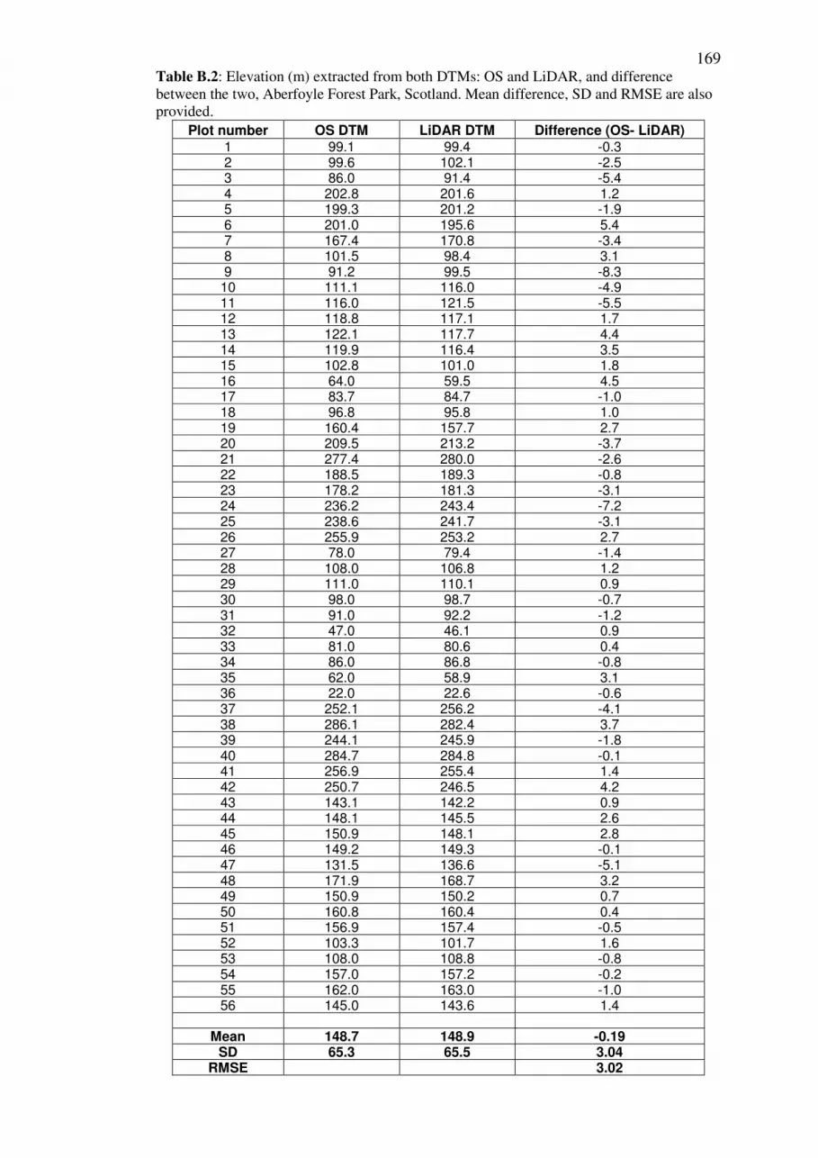
169 Table B.2: Elevation (m) extracted from both DTMs: OS and LiDAR, and difference
between the two, Aberfoyle Forest Park, Scotland. Mean difference, SD and RMSE are also
provided.
Plot number OS DTM LiDAR DTM Difference (OS- LiDAR)
1 99.1 99.4 -0.3 2 99.6 102.1 -2.5 3 86.0 91.4 -5.4 4 202.8 201.6 1.2 5 199.3 201.2 -1.9 6 201.0 195.6 5.4 7 167.4 170.8 -3.4 8 101.5 98.4 3.1 9 91.2 99.5 -8.3 10 111.1 116.0 -4.9 11 116.0 121.5 -5.5 12 118.8 117.1 1.7 13 122.1 117.7 4.4 14 119.9 116.4 3.5 15 102.8 101.0 1.8 16 64.0 59.5 4.5 17 83.7 84.7 -1.0 18 96.8 95.8 1.0 19 160.4 157.7 2.7 20 209.5 213.2 -3.7 21 277.4 280.0 -2.6 22 188.5 189.3 -0.8 23 178.2 181.3 -3.1 24 236.2 243.4 -7.2 25 238.6 241.7 -3.1 26 255.9 253.2 2.7 27 78.0 79.4 -1.4 28 108.0 106.8 1.2 29 111.0 110.1 0.9 30 98.0 98.7 -0.7 31 91.0 92.2 -1.2 32 47.0 46.1 0.9 33 81.0 80.6 0.4 34 86.0 86.8 -0.8 35 62.0 58.9 3.1 36 22.0 22.6 -0.6 37 252.1 256.2 -4.1 38 286.1 282.4 3.7 39 244.1 245.9 -1.8 40 284.7 284.8 -0.1 41 256.9 255.4 1.4 42 250.7 246.5 4.2 43 143.1 142.2 0.9 44 148.1 145.5 2.6 45 150.9 148.1 2.8 46 149.2 149.3 -0.1 47 131.5 136.6 -5.1 48 171.9 168.7 3.2 49 150.9 150.2 0.7 50 160.8 160.4 0.4 51 156.9 157.4 -0.5 52 103.3 101.7 1.6 53 108.0 108.8 -0.8 54 157.0 157.2 -0.2 55 162.0 163.0 -1.0 56 145.0 143.6 1.4
Mean 148.7 148.9 -0.19 SD 65.3 65.5 3.04
RMSE 3.02

170 Table B.3: Mean field canopy closure; mean LiDAR canopy cover and difference
between both, Abernethy Forest, Scotland. Root mean square error (RMSE), mean and
standard deviation (SD) of both LiDAR and field measured canopy density are also
presented. Plot ID
Tree species
% Canopy closure (field)
% Canopy cover (LiDAR)
Difference (field - LiDAR)
1 Scots pine 91.3 86.9 4.4
2 Scots pine 61.5 11.6 49.8
3 Scots pine 91.4 80.0 11.3
4 Scots pine 92.0 86.8 5.2
5 Scots pine 93.2 90.2 3.0
6 Scots pine 93.5 89.2 4.3
7 Scots pine 88.5 74.9 13.6
8 Scots pine 88.0 68.3 19.7
9 Scots pine 89.8 60.4 29.4
10 Scots pine 73.3 18.7 54.6
11 Scots pine 94.8 93.2 1.6
12 Scots pine 94.2 44.1 50.2
13 Scots pine 76.8 13.8 63.0
14 Scots pine 77.2 32.5 44.7
15 Scots pine 91.3 95.7 -4.4
16 Scots pine 92.2 81.1 11.1
17 Scots pine 91.8 77.6 14.2
18 Scots pine 88.6 83.1 5.5
19 Scots pine 92.4 87.0 5.4
20 Scots pine 85.2 55.8 29.4
21 Scots pine 92.9 85.3 7.5
22 Scots pine 91.5 84.4 7.1
23 Scots pine 90.7 84.7 6.0
24 Scots pine 89.0 76.4 12.6
25 Scots pine 93.5 72.2 21.3
26 Scots pine 91.9 74.4 17.6
27 Scots pine 90.7 81.2 9.5
28 Scots pine 90.4 81.0 9.4
29 Scots pine 69.9 42.7 27.3
30 Scots pine 92.6 79.5 13.1
31 Scots pine 91.4 89.6 1.8
32 Scots pine 89.2 65.5 23.7
Mean 88.1 70.2 17.9
SD 7.7 23.1 17.3
RMSE 24.7

171 Table B.4: Mean field canopy closure; mean LiDAR canopy cover and difference
between both, sitka spruce plots- Aberfoyle Forest, Scotland. Root mean square error
(RMSE), mean and standard deviation (SD) of both LiDAR and field measured canopy
density are also presented. Plot ID
Tree species
%Canopy Cover (LiDAR)
% Canopy Closure (Field)
Difference (Field - LiDAR)
1 Sitka spruce 66.9 94.3 27.4
2 Sitka spruce 40.4 93.2 52.8
3 Sitka spruce 45.6 93.8 48.3
4 Sitka spruce 82.6 93.7 11.1
5 Sitka spruce 91.9 93.9 2.0
6 Sitka spruce 82.1 92.5 10.4
7 Sitka spruce 88.1 93.3 5.2
8 Sitka spruce 78.4 93.4 15.0
9 Sitka spruce 81.9 91.8 9.9
10 Sitka spruce 67.8 92.0 24.2
11 Sitka spruce 69.4 91.6 22.2
12 Sitka spruce 70.7 90.9 20.1
13 Sitka spruce 86.3 89.3 2.9
14 Sitka spruce 88.7 91.8 3.1
15 Sitka spruce 83.2 92.4 9.2
16 Sitka spruce 49.3 92.7 43.4
17 Sitka spruce 80.5 87.9 7.4
18 Sitka spruce 65.6 86.5 20.8
19 Sitka spruce 96.0 94.0 -2.1
20 Sitka spruce 99.0 92.2 -6.8
21 Sitka spruce 98.6 94.0 -4.6
22 Sitka spruce 99.5 92.7 -6.8
23 Sitka spruce 100.0 92.9 -7.1
24 Sitka spruce 100.0 94.2 -5.8
25 Sitka spruce 99.4 94.3 -5.1
26 Sitka spruce 100.0 94.5 -5.5
27 Sitka spruce 94.4 91.8 -2.6
28 Sitka spruce 99.6 94.7 -5.0
29 Sitka spruce 88.9 92.5 3.5
30 Sitka spruce 76.5 92.5 15.9
31 Sitka spruce 80.5 91.7 11.2
32 Sitka spruce 95.2 92.7 -2.5 33 Sitka spruce 98.9 93.0 -5.9
34 Sitka spruce 82.1 93.0 10.9 35 Sitka spruce 96.4 93.4 -3.1 36 Sitka spruce 84.1 92.4 8.2
Mean 83.6 92.5 9.0
SD 15.9 1.7 15.5
RMSE 17.7

172 Table B.5: Mean field canopy closure; mean LiDAR canopy cover and difference
between both, Scots pine plots- Aberfoyle Forest, Scotland. Root mean square error
(RMSE), mean and standard deviation (SD) of both LiDAR and field measured canopy
density are also presented. Plot ID Tree species %Canopy Cover
(LiDAR) % Canopy Closure
(Field Difference (Field -
LiDAR)
37 Scots pine 83.5 87.6 4.1
38 Scots pine 57.4 54.4 -3.0
39 Scots pine 88.3 93.1 4.8
40 Scots pine 96.4 90.2 -6.2
41 Scots pine 91.4 93.6 2.2
42 Scots pine 91.4 93.1 1.7
43 Scots pine 57.6 84.4 26.8
44 Scots pine 75.1 86.5 11.5
45 Scots pine 88.1 91.1 3.0
46 Scots pine 70.7 80.7 10.0
47 Scots pine 55.5 83.3 27.8
48 Scots pine 65.3 77.3 11.9
49 Scots pine 52.0 80.0 28.0
50 Scots pine 73.3 88.0 14.7
51 Scots pine 80.4 81.1 0.7
52 Scots pine 78.4 93.8 15.3
53 Scots pine 59.9 84.8 24.9
54 Scots pine 79.3 87.2 7.9
55 Scots pine 79.1 89.6 10.5
56 Scots pine 79.7 87.8 8.1
Mean 75.1 85.4 10.2 SD 13.3 8.7 10.2
RMSE 14.3
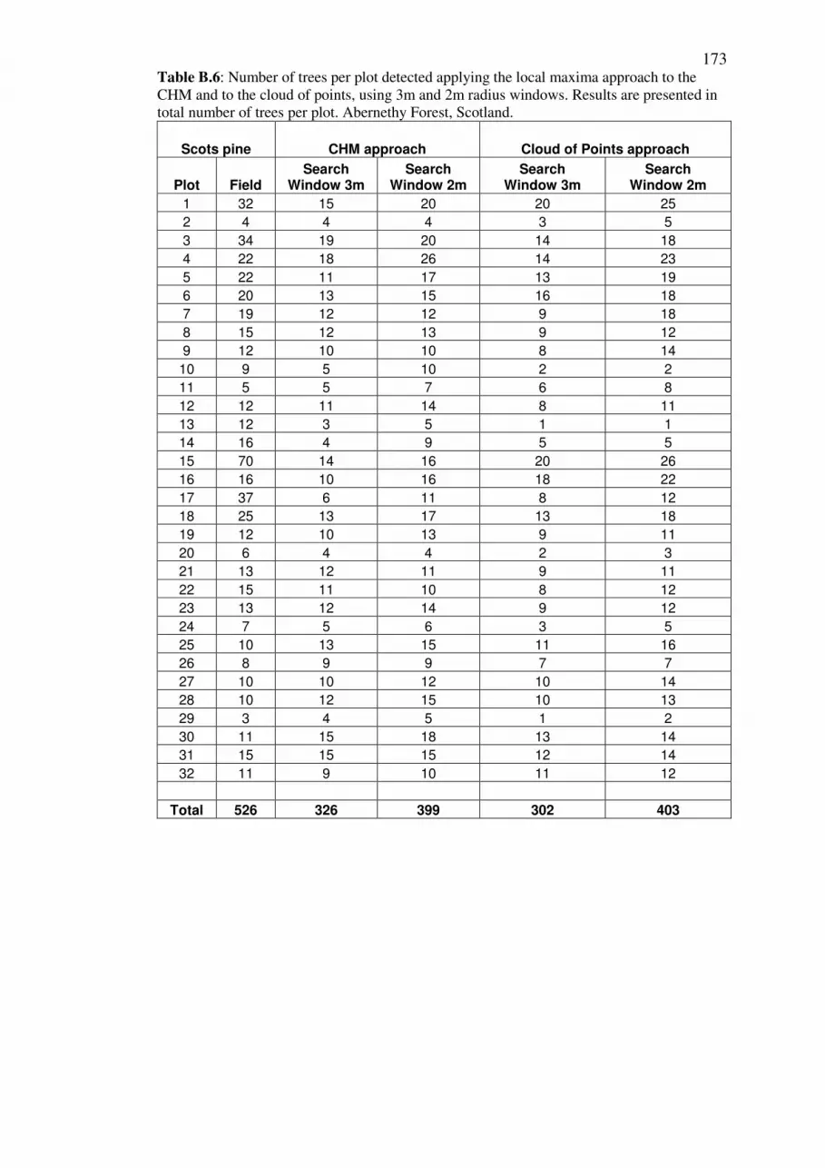
173 Table B.6: Number of trees per plot detected applying the local maxima approach to the
CHM and to the cloud of points, using 3m and 2m radius windows. Results are presented in
total number of trees per plot. Abernethy Forest, Scotland.
Scots pine CHM approach Cloud of Points approach
Plot Field Search
Window 3m Search
Window 2m Search
Window 3m Search
Window 2m
1 32 15 20 20 25
2 4 4 4 3 5
3 34 19 20 14 18
4 22 18 26 14 23
5 22 11 17 13 19
6 20 13 15 16 18
7 19 12 12 9 18
8 15 12 13 9 12
9 12 10 10 8 14
10 9 5 10 2 2
11 5 5 7 6 8
12 12 11 14 8 11
13 12 3 5 1 1
14 16 4 9 5 5
15 70 14 16 20 26
16 16 10 16 18 22
17 37 6 11 8 12
18 25 13 17 13 18
19 12 10 13 9 11
20 6 4 4 2 3
21 13 12 11 9 11
22 15 11 10 8 12
23 13 12 14 9 12
24 7 5 6 3 5
25 10 13 15 11 16
26 8 9 9 7 7
27 10 10 12 10 14
28 10 12 15 10 13
29 3 4 5 1 2
30 11 15 18 13 14
31 15 15 15 12 14
32 11 9 10 11 12
Total 526 326 399 302 403

174 Table B.7: Number of trees per plot detected applying the local maxima algorithm to the
CHM and to the cloud of points, using 3m and 2m radius windows. Results are presented in
total number of trees per plot. (Scots pine plots only) Aberfoyle Forest, Scotland.
Scots pine CHM approach Cloud of Points approach
Plot Field Search
Window 3m Search
Window 2m Search
Window 3m Search
Window 2m
1 14 6 8 6 8
2 13 1 2 1 3
3 7 5 9 5 6
4 22 4 4 5 9
5 18 3 9 5 9
6 18 5 12 7 11
7 9 3 6 3 5
8 11 5 7 5 9
9 16 6 12 5 9
10 11 2 5 4 8
11 12 5 8 3 9
12 8 4 5 4 6
13 9 4 6 4 5
14 9 3 8 2 5
15 12 1 4 6 7
16 28 6 13 4 9
17 30 5 9 5 8
18 30 2 6 6 7
19 36 6 10 6 10
20 11 5 9 5 10
Total 324 81 152 91 153

175 Table B.8: Number of trees per plot detected applying the local maxima algorithm to the
CHM and to the cloud of points, using 3m and 2m radius windows. Results are presented in
total number of trees per plot. (sitka spruce plots only) Aberfoyle Forest, Scotland.
Sitka spruce CHM approach Cloud of Points approach
Plot Field Search
Window 3m Search
Window 2m Search
Window 3m Search
Window 2m
1 49 3 5 4 9
2 22 1 2 2 4
3 9 2 2 2 3
4 3 3 4 3 4
5 4 2 3 3 4
6 5 4 4 4 7
7 5 1 6 2 5
8 21 3 6 3 7
9 8 5 7 5 5
10 9 4 8 5 8
11 5 3 10 3 5
12 16 3 6 4 5
13 5 3 8 4 7
14 7 2 7 2 7
15 5 2 4 3 4
16 8 2 3 1 2
17 7 3 8 3 9
18 6 2 3 2 5
19 38 6 7 8 8
20 49 2 10 7 9
21 70 8 15 7 15
22 30 6 10 4 10
23 38 5 8 4 8
24 67 5 12 5 9
25 73 4 12 5 13
26 83 4 14 5 6
27 36 6 12 4 7
28 46 5 8 6 10
29 10 3 9 6 7
30 22 2 7 5 7
31 15 3 10 5 12
32 28 3 10 4 8
33 64 8 10 7 13
34 12 5 8 6 8
35 7 4 10 4 10
36 8 4 4 4 9
Total 890 131 272 151 269

176 Table B.9: Field mean height and LiDAR 90
th & 95
th percentile canopy height -values
per plot. Average and SD. Abernethy Forest, Scotland
Plot ID
Tree Species
Field field mean
height LiDAR
90th
percentile
LiDAR 95th
percentile
1 Scots pine 20.3 18.4 18.4
2 Scots pine 15.2 15.3 14.6
3 Scots pine 16.1 18.2 17.2
4 Scots pine 22.4 19.4 18.5
5 Scots pine 19.5 18.2 18.7
6 Scots pine 22.9 18.6 19.3
7 Scots pine 21.1 17.6 18.1
8 Scots pine 20.6 18.2 18.6
9 Scots pine 21.6 19.1 19.8
10 Scots pine 7.5 8 6.7
11 Scots pine 24.5 21.5 20.5
12 Scots pine 12.6 11.3 10.6
13 Scots pine 13.5 10 7.4
14 Scots pine 12.7 11 12.6
15 Scots pine 17.9 17.2 17
16 Scots pine 15.9 13.5 13.9
17 Scots pine 13.9 12.1 13
18 Scots pine 14.6 13.1 13.5
19 Scots pine 17.2 17.1 16.8
20 Scots pine 18.3 16.3 17.1
21 Scots pine 20.2 17.5 17.9
22 Scots pine 15.6 13.1 14.4
23 Scots pine 20.1 17.6 19.3
24 Scots pine 19.2 13.6 14.1
25 Scots pine 21.1 17.9 18.3
26 Scots pine 20.5 17.1 19
27 Scots pine 21.9 16.9 18.3
28 Scots pine 22.8 19.7 19.2
29 Scots pine 20.4 17.1 16.3
30 Scots pine 19.4 18.7 19
31 Scots pine 24.5 21.9 21.9
32 Scots pine 19.1 17.5 18.5
Mean 18.5 16.3 16.5
SD 3.9 3.3 3.6

177 Table B.10: Field mean height and LiDAR 90
th & 95
th percentile canopy height -values
per plot. Average and SD. Aberfoyle Forest, Scotland
Plot ID Tree species Field mean height LiDAR 90th percentile
LiDAR 95th percentile
1 Sitka spruce 25.0 19.5 20.1 2 Sitka spruce 27.3 23.0 29.1
3 Sitka spruce 35.0 20.0 35.8 4 Sitka spruce 34.2 32.0 36.4
5 Sitka spruce 37.5 32.0 34.3 6 Sitka spruce 43.7 35.3 32.7 7 Sitka spruce 36.9 31.0 32.4
8 Sitka spruce 36.9 30.5 33.7 9 Sitka spruce 33.1 32.0 32.0
10 Sitka spruce 32.9 28.0 30.0 11 Sitka spruce 33.7 30.0 31.7 12 Sitka spruce 20.8 19.5 17.9
13 Sitka spruce 36.2 31.2 33.2 14 Sitka spruce 31.0 31.6 30.3
15 Sitka spruce 31.1 31.8 31.7 16 Sitka spruce 40.1 33.7 37.7 17 Sitka spruce 33.2 28.6 34.2
18 Sitka spruce 37.2 29.8 36.8 19 Sitka spruce 37.0 29.3 31.9
20 Sitka spruce 25.5 23.3 24.0 21 Sitka spruce 19.9 17.7 19.0 22 Sitka spruce 31.0 29.6 30.2
23 Sitka spruce 29.7 28.8 28.7 24 Sitka spruce 27.6 24.7 26.0
25 Sitka spruce 24.8 21.6 22.6 26 Sitka spruce 29.3 24.8 27.9
27 Sitka spruce 23.5 21.0 22.4 28 Sitka spruce 24.4 23.0 23.3 29 Sitka spruce 23.8 20.4 23.9
30 Sitka spruce 25.0 20.0 23.3 31 Sitka spruce 24.6 18.7 21.8
32 Sitka spruce 28.0 22.3 24.4 33 Sitka spruce 24.7 21.4 22.2 34 Sitka spruce 25.0 20.8 22.4
35 Sitka spruce 30.5 27.8 30.1 36 Sitka spruce 26.4 22.5 24.8
37 Scots pine 23.0 22.7 23.2 38 Scots pine 17.5 21.0 21.6 39 Scots pine 22.3 20.9 22.3
40 Scots pine 15.6 16.6 19.4 41 Scots pine 21.0 19.4 21.7
42 Scots pine 19.2 18.6 21.5 43 Scots pine 24.1 19.3 20.5 44 Scots pine 22.7 18.6 21.5
45 Scots pine 21.3 19.2 20.3 46 Scots pine 21.7 20.8 21.9
47 Scots pine 21.5 19.8 20.0 48 Scots pine 21.9 19.7 20.6
49 Scots pine 21.7 17.0 20.4 50 Scots pine 23.3 19.1 22.1 51 Scots pine 22.8 18.8 21.0
52 Scots pine 18.5 18.0 18.3 53 Scots pine 16.2 16.9 16.9
54 Scots pine 19.5 15.3 16.6 55 Scots pine 17.1 15.5 18.1 56 Scots pine 21.4 20.0 20.5
Mean 26.8 23.5 25.5
SD 6.7 5.5 5.9

178
APPENDIX C – GLM validation – Tables
____________________________________________________________________
Table C.1: Field-predicted number of stripped cones, LiDAR-predicted number of stripped
cones and difference between both. Mean values, standard deviation and RMSE. Abernethy
Forest, Scotland.
Plot ID
Field-predicted
cones
LiDAR-predicted
cones
Diff Field-LiDAR
1 16 28 -11
2 1 0 1
3 14 19 -4
4 28 21 7
5 17 15 2
6 40 17 22
7 16 3 12
8 18 4 15
9 19 7 12
10 1 0 1
11 24 26 -2
12 11 0 11
13 3 0 3
14 2 1 2
15 45 1 44
16 18 10 9
17 28 5 23
18 15 14 1
19 13 9 4
20 8 4 4
21 24 13 12
22 17 4 14
23 15 10 5
24 11 4 7
25 16 7 9
26 14 2 12
27 21 9 12
28 15 11 4
29 2 1 1
30 19 13 6
31 27 32 -5
32 15 8 7
Mean 17 9.2 7.5
SD 10 8.6 9.9
RMSE 12.3

179 Table C.2: Field-predicted number of stripped cones, LiDAR-predicted number of cones
using un-calibrated LiDAR number of trees (GLM 1) and calibrated number of trees (GLM
2). Difference between Field and GLM 1 and Field and GLM 2.Mean values, standard
deviation and RMSE. Aberfoyle Forest, Scotland.
Plot ID Field-predicted
cones
LiDAR-predicted
cones GLM 1
LiDAR-predicted
cones GLM 2
Diff Field- GLM 1
Diff Field - GLM2
33 18 25 11 -7.0 7.1
34 1 7 2 -6.0 -0.7
35 27 47 147 -20.0 -119.9
36 14 20 41 -6.0 -26.8
37 29 50 31 -21.0 -1.9
38 38 23 72 15.0 -34.3
39 9 11 3 -2.0 6.4
40 22 7 7 15.0 15.1
41 21 3 23 18.0 -2.5
42 9 32 15 -23.0 -5.7
43 10 5 13 5.0 -3.4
44 8 2 3 6.0 4.6
45 9 1 0 8.0 9.0
46 15 3 12 12.0 3.2
47 11 5 1 6.0 9.8
48 40 33 27 7.0 12.7
49 10 0 0 10.0 10.0
50 13 16 18 -3.0 -5.0
51 17 8 4 9.0 13.0
52 9 5 29 4.0 -20.5
Mean 16.5 15.2 23 1.4 -6.5
SD 10.3 15.3 34 12.1 29.8
RMSE 11.9 29.8

180 Table C.3: Number of cones stripped by squirrels observed in the field and predicted
using field data (LOO cross-validation). Abernethy Forest (plots 1 to 32) and Aberfoyle
(plots 33 to 52)- Scotland
Plot Id
Field-observed stripped cones
Field-predicted stripped cones
(LOO cross-validation)
Difference (Field-observed – Field-predicted)
1 61 16 45
2 4 1 3
3 15 14 1
4 9 28 -19
5 42 17 25
6 4 40 -36
7 12 16 -4
8 27 18 9
9 0 19 -19
10 4 1 3
11 91 24 67
12 20 11 9
13 5 3 2
14 14 2 12
15 35 45 -10
16 11 18 -7
17 47 28 19
18 17 15 2
19 16 13 3
20 0 8 -8
21 44 24 20
22 18 17 1
23 9 15 -6
24 16 11 5
25 60 16 44
26 3 14 -11
27 5 21 -16
28 5 15 -10
29 2 2 0
30 32 19 13
31 55 27 28
32 3 15 -12
33 18 18 0
34 0 1 -1
35 11 27 -16
36 0 14 -14
37 6 29 -23
38 4 38 -34
39 0 9 -9
40 48 22 26
41 7 21 -14
42 2 9 -7
43 3 10 -7
44 2 8 -6
45 21 9 12
46 22 15 7
47 4 11 -7
48 1 40 -39
49 3 10 -7
50 25 13 12
51 57 17 40
52 12 9 3
Mean 17.9 16.6 1.33
SD 20.4 10.0 20.2
RMSE 20.0

181
APPENDIX D – VORTEX predictions – Abernethy Forest ____________________________________________________________________
Table D.1: VORTEX predictions for red squirrel populations at Abernethy Forest: Annual
population size and standard deviation (SD) for Population 1 and Population 2, for each
scenario Basic and LiDAR and for each sub-scenario: catastrophe and no-catastrophe
Population 1
(No-Catastrophe) Population 2
(No-Catastrophe)
Year Basic
Pop Size
Basic-SD LiDAR
Pop Size LiDAR-SD Basic
Pop Size Basic-SD LiDAR
Pop Size LiDAR-SD
1 260 90.3 87 42.6 254 78.4 78 21.2
2 228 112.3 77 44.8 217 104.7 60 30.6
3 202 117.4 62 46.6 197 109.2 56 32.7
4 179 120.0 57 45.8 172 112.5 48 34.0
5 162 122.7 49 47.1 160 115.6 44 34.8
6 146 121.5 46 46.3 140 116.1 38 34.3
7 136 120.9 38 42.2 132 114.8 35 34.2
8 124 118.8 37 43.8 122 113.0 30 33.0
9 110 117.2 31 41.0 107 111.9 30 33.5
10 104 110.7 30 39.4 101 106.6 24 30.8
11 92 110.0 25 38.6 89 108.1 23 31.4
12 82 110.8 24 38.5 81 104.3 20 30.0
13 75 103.0 20 34.2 74 100.2 19 28.7
14 69 104.5 20 35.7 67 101.4 17 28.2
15 62 101.3 18 34.3 62 96.2 16 27.7
16 57 98.8 17 32.6 56 95.1 15 27.3
17 49 100.8 17 34.4 49 93.0 16 27.7
18 45 101.9 16 33.4 44 99.1 13 25.6
19 42 99.2 13 29.2 42 94.8 13 25.5
20 42 95.0 13 30.2 42 91.8 11 24.1
Population 1 (Catastrophe)
Population 2 (Catastrophe)
Year Basic
Pop Size
Basic-SD LiDAR
Pop Size LiDAR-SD Basic
Pop Size Basic-SD LiDAR
Pop Size LiDAR-SD
1 242 98.0 87 43.9 238 86.6 76 22.5
2 203 113.2 74 45.1 194 106.5 59 31.2
3 171 118.1 60 45.2 169 110.6 54 32.4
4 157 118.0 55 46.2 150 111.6 45 33.8
5 133 116.3 47 44.9 133 111.6 42 33.9
6 122 118.1 44 44.8 116 110.5 37 33.7
7 114 117.1 37 41.9 112 112.9 34 33.2
8 103 114.7 35 42.2 101 109.6 30 33.2
9 97 114.1 32 41.0 94 109.2 28 32.2
10 92 114.4 27 36.0 89 107.9 25 31.6
11 84 110.0 25 38.0 82 107.3 21 29.2
12 79 108.4 23 36.1 79 104.6 22 30.5
13 70 101.6 22 37.1 69 99.9 20 29.6
14 63 98.4 18 33.1 63 95.8 17 27.9
15 59 97.8 18 33.4 58 95.2 16 27.7
16 56 95.1 15 30.0 54 91.3 14 25.2
17 53 95.3 14 28.1 52 92.5 13 25.1
18 47 89.7 14 30.9 46 85.1 13 25.6
19 44 86.7 12 27.7 43 84.6 11 25.4
20 38 78.5 11 29.7 37 75.1 9 22.3

182
APPENDIX E – Related publications
____________________________________________________________________
The following publications contain work related to or derived from this thesis.
Peer-reviewed publications
Flaherty, S.; Patenaude, G., Close A. & Lurz, P. 2012. The impact of forest-stand
structure on red squirrel habitat use, Forestry: An International Journal of Forest
Research, Vol. 85, No.3, pp 437-444
Conference proceedings
Flaherty, S.; Patenaude, G., & Lurz, P. The use of LiDAR remote sensing for red
squirrel habitat mapping in Abernethy Forest, Scotland. In Proceedings of ForestSat
2010, 7th -9th September, Lugo, Spain
Flaherty, S.; Lurz, P. & Patenaude, G. Implementation of a General Linear Model
using LiDAR derived explanatory variables: a case study in Scotland. In
Proceedings of SPIE Remote Sensing, 24 - 27 September 2012, Edinburgh, United
Kingdom (Submitted)
In preparation
Flaherty, S.; Lurz, P. & Patenaude, G. Red squirrel habitat mapping using LiDAR
remote sensing. To be submitted to the Journal of Applied Remote Sensing
Zuur, A.F.; Flaherty, S.; Lurz, P.; Patenaude, G., Ieno, E.N.; Hilbe, J. Generalized
linear modelling with MCMC in JAGS applied to red squirrel data; In A Beginner's
guide to GLM using R and JAGS , Zuur, A.F.; Ieno, E.N.; Hilbe, J.