Energies 2014, 7, 2850-2873; doi:10.3390/en7052850

energies ISSN 1996-1073

www.mdpi.com/journal/energies

Article

Energy Substitution, Technical Change and Rebound Effects

Steve Sorrell

Centre for Innovation and Energy Demand and Sussex Energy Group,

SPRU—Science and Technology Policy Research, University of Sussex, Falmer, Brighton BN1 9QE, UK;

E-Mail: s.r.sorrell@sussex.ac.uk; Tel.: +441-273-877-067; Fax: +441-273-685-865

Received: 28 February 2014; in revised form: 13 April 2014 / Accepted: 16 April 2014 /

Published: 29 April 2014

Abstract: This paper investigates the relationships between energy efficiency

improvements by producers, the ease of substitution between energy and other inputs and

the size of the resulting “rebound effects”. Fundamentally, easier substitution leads to

larger rebounds. Focusing upon conceptual and methodological issues, the paper highlights

the challenges of estimating and modeling rebound effects with the help of production and

cost functions and questions the robustness of the evidence base in this area. It argues that

the multiple definitions of “elasticities of substitution” are a source of confusion, the most

commonly estimated elasticity is of little practical value, the empirical literature is

contradictory, prone to bias and difficult to use and there are only tenuous links between

this literature and the assumptions used within energy-economic models. While

“energy-augmenting technical change” provides the natural choice of independent variable

for an estimate of rebound effects, most empirical studies do not estimate this form of

technical change, many modeling studies do not simulate it and others simulate it in such a

way as to underestimate rebound effects. As a result, the paper argues that current

econometric and modeling studies do not provide reliable guidance on the magnitude of

rebound effects in different industrial sectors.

Keywords: rebound effects; elasticities of substitution; energy augmenting technical change

1. Introduction

The “rebound effect” is an umbrella term for a variety of economic mechanisms that reduce the

“energy savings” from improved energy efficiency [1]. For producers, cost-effective energy efficiency

improvements encourage increased consumption of energy services, boost productivity, increase

OPEN ACCESS

Energies 2014, 7 2851

output and potentially impact energy use throughout the economy. The rebound effect is commonly

defined as the percentage of potential energy savings that are offset by these different mechanisms.

For producers, the potential energy savings are typically estimated by engineering models that assume

no economic responses to improved energy efficiency, while “actual” savings are estimated by

energy-economic models that simulate those responses with the help of econometrically estimated

production or cost functions [1–4].

Energy efficiency or energy productivity may generally be defined as the ratio of useful outputs to

energy inputs for a specified system. Inputs and outputs may be defined in thermodynamic, physical or

economic terms [5] and different definitions and measures, as well as different choices of system

boundary, may lead to different conclusions regarding the nature, source, magnitude and sign of

energy productivity improvements, as well as of the energy savings that result. But neoclassical

production theory narrows the range of choices for these variables: defining energy productivity solely

in economic terms and focusing upon only two sources of energy productivity improvements: namely

the substitution of energy by other inputs and technical change. The latter provides a common choice

of independent variable for studies of rebound effects in industrial production [3,6].

In a widely cited paper, Saunders [7] uses neoclassical production theory to argue that: “… the ease

with which fuel can substitute for other factors of production (such as capital and labour) has a strong

influence on how much rebound will be experienced … the greater this ease of substitution, the greater

will be the rebound”. Saunders [2,8–11] had extended this analysis in subsequent works, but consistently

concludes that rebound effects will be larger when “…the greater is the flexibility of the economy to

adapt to energy efficiency gains via substitution” [10]. Saunders’ results therefore imply that empirical

studies of the “ease of substitution” between energy and other inputs should allow the likely magnitude

of rebound effects in different sectors to be explored [7].

This paper investigates the relationships between energy productivity improvements for producers,

the ease of substitution between energy and other inputs and the size of the resulting rebound

effects. It assesses the meaning and applicability of the above statement by Saunders [7], the challenge

of estimating and modeling rebound effects with production and cost functions and the robustness of

the evidence base in this area. The paper focuses on conceptual and methodological issues, partly with

the aim of clarifying these issues for non-specialists.

The paper begins by outlining how different types of energy productivity improvement are

represented in neoclassical production theory, how these may lead to rebound effects and how

energy substitution contributes to those effects. The following three sections examine how the “ease of

substitution” between energy and other inputs is defined and measured and how these estimates are

commonly used. The paper highlights the challenges in estimating “elasticities of substitution”, the

difficulties in interpreting the available literature, the contradictions in the empirical results and the

tenuous link between these results and the assumptions used in energy-economic models. Section 8

compares the different ways of estimating and modeling technical change and highlights the

limitations of commonly used measures when applied to the estimation of rebound effects. On the

basis of these arguments, the paper argues that current econometric and modeling studies do not

provide reliable guidance on the magnitude of rebound effects in different sectors. The paper

concludes by indicating the requirements for providing more realistic guidance.

Energies 2014, 7 2852

2. Key Concepts from Production Theory

Neoclassical production functions indicate the maximum possible economic output (Y) obtainable

from capital (K), labor (L) and intermediate inputs to a firm or sector given the technology available at

a particular time (t) [12]. Intermediates are commonly disaggregated into energy (E) and materials (M)

(while consistent with the structure of input-output tables, the treatment of capital and labor as primary

inputs and energy as a secondary or intermediate input is problematic from the perspective of the

natural sciences):

),,,,( tMELKfY = (1)

Production functions are normally assumed to be positive, twice differentiable and quasi-concave

with constant returns to scale. Under standard assumptions a dual cost function can be defined which

indicates the minimum possible cost (C) of producing output Y, given the prices of each input (pi)

and the current state of technology (t):

),,,,,( tYppppgC MELK= (2)

Dividing through by output gives a unit cost function (c = C/Y):

),,,,( tpppphc MELK= (3)

Cost functions are preferred to production functions in empirical studies since the independent

variables (input prices) are more likely to be exogenous.

Assuming perfect competition and profit maximization, the marginal product of each input should

be equal to the input price (pi) and the elasticity of cost with respect to this price should be equal to the

“value share” (si):

ii

pX

Y =∂∂

(4)

ii

sp

C =∂∂ln

ln (5)

where:

C

Xps iii = (6)

The output produced from a given quantity of inputs typically increases over time as technology

improves. The rate of change of total factor productivity (εft) is then given by:

ft

lnε

Y

t

∂=∂

(7)

The equivalent cost function definition is:

gt

lnε

C

t

∂= −∂

(8)

With constant returns to scale: εft = εgt.

Energies 2014, 7 2853

Energy productivity (θE) is defined as the ratio of economic output to energy inputs: ( , , , , )

θE

Y f K L E M t

E E= = (9)

Aggregate energy productivity therefore depends upon the level of each input, the current state of

technology and the level of output, as well as upon how individual inputs are measured and aggregated

(e.g., how different types of energy carrier are combined). The inverse of energy productivity

(energy intensity) can be derived from the unit cost function using Shephard’s Lemma:

1

θE E

c E

p Y

∂ = =∂

(10)

Increases in energy prices encourage the substitution of other inputs for energy, thereby improving

aggregate energy productivity but since costs have increased output may fall. In contrast, technical

change is assumed to improve energy productivity independently of changes in relative prices and

without reducing output. Total factor productivity measures the net impact of technical change on

all inputs. Technical change has frequently been assumed to be time-dependent, exogenous and neutral

(N), with the productivity of all inputs increasing at the same constant rate (εft = λN ≥ 0). In this form,

technical change may be represented as a time-dependent multiplier on the production function:

τ ( , , , )NY f K L E M= (11)

where: λτ ( ) N t

N t e= (12)

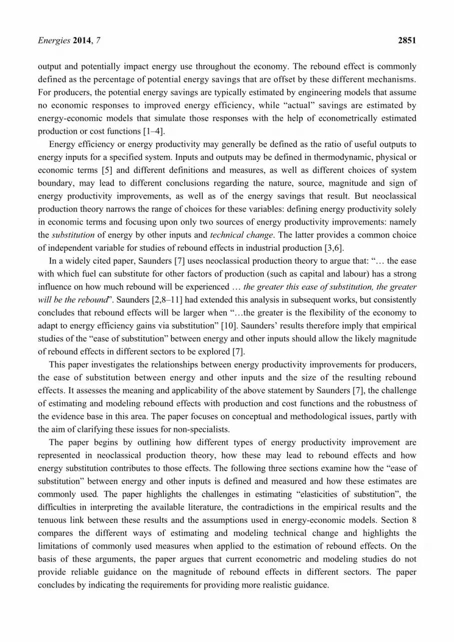
Substitution is conventionally represented as movement along an isoquant of a production or cost

function and technical change as a shift of the isoquants (Figure 1). However, the distinction between

the two is less clear from an engineering perspective and both may reflect a complex mix of

investment, operational changes and shifts in the composition of output [13].

Figure 1. Substitution and neutral technical change.

In practice, technical change is frequently biased in that the productivity of some inputs increases

more rapidly than others [12]. In empirical studies, this is commonly measured by the rate of change in

the value share of each input, independent of changes in relative prices:

Other inputs - X

Energy - E

Substitution

Technical change

Y

Y

Energies 2014, 7 2854

ψ ii

s

t

∂=∂

(13)

Technical change is said to be “input saving” if the value share of that input falls over time (ψi < 0) and “input using” if it increases (ψi > 0) [14,15]. Note that ψ 1i

i

= .

In modeling studies, biases in technical change are commonly simulated by including “augmenting multipliers” ( λτ ( ) it

i t e= where λi > 0) on one or more inputs to the production function:

(τ , τ , τ , τ )K L E MY f K L E M= (14)

Letting τi i iX X= , this can be expressed as:

),,(~~~~~

MELKfY = (15)

Letting / τi iip p= , the equivalent effective cost function is:

),,,(~ ~~~~MELK ppppgC = (16)

The “effective production function” (~

f ) indicates the maximum output obtainable from the

effective ( iX~

) rather than real inputs. “Input-augmenting technical change” is defined as / τ 0iY∂ ∂ > ;

implying that the marginal productivity of input Xi increases over time and its “effective price” ( ip~ )

falls. The energy-augmenting multiplier (τE) converts energy inputs (E) to “effective energy” ( E~ ).

Although the latter is sometimes referred to as “energy services”, it is different from the engineering

interpretation of that term.

A key point relevant to the estimation of rebound effects is that “energy-augmenting” technical

change is not the same as “energy saving” technical change. As described below, the former may not

lead to the latter owing to substitution between inputs. Also, the direction of technical change is likely

to be influenced by relative prices.

3. Technical Change, Energy Substitution and Rebound Effects

Saunders [7] defined rebound effects in relation to energy-augmenting technical change (τE).

This represents a “pure” energy productivity improvement that does not affect the productivity of

other inputs or negatively affect economic output. But as described below, empirical studies may not

directly estimate this form of technical change, energy-economic models may not simulate it (or may

simulate it in different ways) and studies of rebound effects may make a different choice for the

independent variable. Also, isolating energy-augmenting technical change in this way is somewhat

artificial as new technologies frequently improve the productivity of multiple inputs simultaneously.

In general, energy-augmenting technical change will not lead to a proportionate improvement in

aggregate energy productivity (θE) because:

• lower price effective energy will stimulate the substitution of (effective) energy for other

(effective) inputs; and

• lower input costs will stimulate an increase in output which in turn will “drag up”

energy consumption.

Energies 2014, 7 2855

In combination, these substitution and output effects will increase energy consumption above what

it would have been in the absence of these responses. The sum of the two is the direct rebound effect

for producers. In addition, there will also be various indirect and economy-wide rebound effects.

For example, if the relevant product forms an intermediate input to other sectors (e.g., steel in car

production), reductions in product prices may stimulate increased output from those sectors and hence

further increase economy-wide energy consumption. But this paper is concerned solely with direct

rebound effects.

The contribution of substitution to the direct rebound effect may be illustrated graphically.

For simplicity, we assume that non-energy inputs are “separable” from energy inputs and can therefore

be grouped together, or “nested”. The meaning and implications of this assumption are described

further below. Figure 2 shows a two-input conventional production function, where the optimal mix of

energy (E) and a “nest” of other inputs (N) to produce output Y for an expenditure of C is given by

the intersection of the isoquants with the iso-cost line (N0, E0). Energy-saving technical change shifts

the isoquants to the left and changes their slope. If other inputs remain unchanged, the potential energy

savings are E0 − E1. However, over time producers will shift to a new, lower cost input mix (N1, E2),

leading to actual energy savings of E0 − E2 which are less than the potential savings. The size of

the rebound effect ((E2 − E1)/(E0 − E1)) depends upon the ease of substitution between energy and

other inputs—indicated by the curvature of the isoquant.

Figure 2. Energy-augmenting technical change encourages the substitution of energy for

other inputs.

Technical change may also increase output (not shown) since: first, a higher level of output can be

produced for a given expenditure on inputs; and second, reductions in product prices may increase

aggregate supply and hence output. This increase in output will further increase energy use. The total

direct rebound effect is the sum of these substitution and output effects. In what follows, we focus on

the substitution effect—which Saunders [11] found to be more important.

4. Rebound Effects with a Constant Elasticity of Substitution (CES) Production Function

These examples illustrate the importance of substitution for rebound effects and suggest that

these effects will be larger when the scope of substitution between energy and other inputs is easier.

Saunders [10] demonstrates this formally, using the following definition of the direct rebound effect (R):

Energies 2014, 7 2856

)(η1 τ ERE

+= (17)

where )(η EEτ is the elasticity of energy consumption with respect to energy-augmenting technical change:

E

EE

E τln

ln)(ητ ∂

∂= (18)

We expect 1)(η0 τ −≥≥ EE

and hence 0 ≤ R ≤ 1. But the direct rebound effect could

theoretically exceed unity (“backfire”) or be negative (“super conservation”). Since E = Y/θE,

Equation (18) can be decomposed:

)(η)(η)(η τττ EθYEEEE

−= (19)

If τη (θ ) 1E E ≤ , there is a substitution effect; and if 0)(ητ ≥Y

E, there is an output effect. Saunders [9]

derived these elasticities for a variety of production and cost functions, but his original analysis [7]

employed a CES production function similar to that used in the majority of energy-economic models.

The particular formulation rests upon the assumption that capital and labor are separable from energy

and may therefore be grouped together:

{ }1

ρ ργ 1 γ ρ( ) ( ) ) (τ )N EY a K L b Eυ − = + (20)

As shown in [9], the substitution, output and rebound effects are (Appendix 1 derives the

substitution effect):

τη (θ) 1 σE

= − (21)

EsY

E −=

1

σ)(ητ (22)

EsR

−=

1

σ

(23)

where σ = 1/(1 − ρ) is the Hicks elasticity of substitution (HES) between the capital-labour composite

and effective energy—a standard measure of the ease of substitution. If σ = 0, there is no rebound effect;

while if σ > 1, energy-augmenting technical change reduces aggregate energy productivity (Δθ < 1)

and increases energy consumption (ΔE > 1). This appears unlikely, since it implies that energy is

a non-essential input. But Saunders [7] demonstrates that alternative “nesting structures” of the same

function (i.e., (KE)L and (LE)K) always lead to rebound effects greater than 100%, regardless of

the HES between the nests. Hence, the estimated magnitude of rebound effects appears sensitive to

the particular choice of nesting structure and functional form.

This discussion suggests that sectors where substitution towards energy is easier (i.e., σ is larger)

will be more vulnerable to rebound effects. Hogan and Manne [16] used analogous arguments to

suggest that sectors where substitution away from energy is easier will be less vulnerable to rising

energy prices. Both conclusions have important policy implications and highlight the importance of

accurately estimating both the ease of substitution and the rate of energy-augmenting technical change

in different sectors.

Energies 2014, 7 2857

So does the existing evidence base allow the ease of substitution and rate of energy-augmenting

technical change within different sectors to be accurately identified? How well do energy-economic

models reflect this evidence base? And can the available empirical and modeling studies provide

reliable guidance on the magnitude of rebound effects in different sectors? The remainder of the paper

addresses these questions by examining: first, the definition and estimation of energy substitution

(Sections 5 and 6); second, the use of those estimates within energy-economic models (Section 7);

and third, the estimation and representation of energy-augmenting technical change (Section 8).

5. Defining Substitution–the Choice of Measure

We first look more closely at how the “ease of substitution” is defined. The previous discussion

used the Hicks elasticity of substitution (σ or HES) which measures the ease with which a decrease

in one input (i) can be compensated by an increase in another (j) while holding output fixed [17].

It is defined as:

ln( / )

ln(π / π )i j

ijj i

X XHES

∂= −

∂ (24)

where πi is the marginal productivity of input Xi )/( iXY ∂∂ . This definition refers to movement along

an isoquant of a production function and is a scale-free measure of the curvature of this isoquant: the

less the curvature the easier it is to substitute between two inputs and the larger the HES (HESij ≥ 0).

The extremes are: a linear production function ( ∞=ijHES ) and a Leontief (fixed proportions)

production function (HESij = 0). For a Cobb Douglas production function HES = 1, while for a CES

production function, HES is constant (as the name suggests) between 0 and infinity. If HESij > 1,

each input can fully substitute for the other (i.e., the isoquants cross the axes). Assuming profit

maximization and perfect competition, the HES can also be defined in relation to a change in

relative prices:

)/ln(

)/ln(

ij

jiij pp

XXHES

∂∂

= (25)

The HES was originally defined for a two-input production function (capital and labor). When applied

to multi-input production functions it is sometimes termed the Hicks Allen elasticity of substitution (HAES),

but this extension creates difficulties since the ease of substitution between i and j may depend upon

the level or price of other inputs. This may not be the case if i and j are separable from other inputs but,

as discussed below, this assumption often does not hold. Also, the value of the HAES depends upon the

particular price changes being considered. For this reason, most empirical studies define substitution in

relation to changes in a single input price, with the most common measures being the Cross price

elasticity (CPEij), the Allen-Uzawa elasticity of substitution (AESij) and the Morishima elasticity of

substitution (MESij). The relevant definitions are given in Table 1 and Box 1. Substitution between two

inputs is easier when these measures are larger and their sign is commonly used to define inputs as

either substitutes (+ve) or complements (−ve). However, whether two inputs may be described as

substitutes or complements depends upon the particular elasticity that is being used. This, together with

inconsistent terminology, complicates the interpretation of the empirical literature.

Energies 2014, 7 2858

Table 1. Comparing common definitions of substitution elasticities. Source: Broadstock et al. [18].

Definition Output Other inputs

jik XX ,≠ Other input prices

jik pp ,≠ Type Substitutes

(complements) Input shares

≤≥

1 Symmetric

)/ln(

)/ln(

ij

jiij

XXHES

ππ∂∂

−=

)/ln(

)/ln(

ij

jiij pp

XXHES

∂∂

= Fixed Fixed Fixed Two input, two price HESij > 0 0

)/(

)/(

≤≥

∂∂

ji

ji

XX

ss Yes

)/ln(

)/ln(

ij

jiij pp

XXHAES

∂∂

= Fixed Variable Fixed Two input, two price HAESij > 0 (<0) 0)/(

)/(

≤≥

∂∂

ji

ji

XX

ss No

j

iij p

XCPE

ln

ln

∂∂= Fixed Variable Fixed One input, one price CPEij > 0 (<0) 0

ln

ln

≤≥

∂∂

j

i

p

s No

j

i

jij p

X

sAES

ln

ln1

∂∂= Fixed Variable Fixed One input, one price AESij > 0 (<0) 0

ln

ln

≤≥

∂∂

j

i

p

s Yes

)ln(

)/ln(

j

jiij p

XXMES

∂∂

= Fixed Variable Fixed Two input, one price MESij > 0 (<0) 0ln

)/ln(

≤≥

∂∂

j

ji

p

ss No

Note: Xi = level of input i; pi = unit price of input i; πi = marginal productivity of input i ( ixf ∂∂ / ); and si = share of i in input costs (si = Xipi/C). Under perfect competition,

si is equal to the share of i in the value of output.

Energies 2014, 7 2859

Box 1. Relationships among common substitution elasticities.

j

ijij s

CPEAES =

jjijij CPECPEMES −=

∂

∂−

∂

∂=

i

j

iji

i

j

jijij

p

pp

MES

p

p

pMESHAES

ln

ln

ln

ln

)1(ln

ln −=∂∂

ijjj

i AESsp

s

)1(ln

)/ln(−=

∂∂

ijj

ji MESp

ss

Source: Broadstock et al. [18], Frondel [19,20], Sato and Koizumi [21]. If only pj changes and pi is fixed,

then HAESij = MESij, while if only pi changes and pj is fixed, then HAESij = MESji.

The great majority of empirical studies estimates the AES and uses its sign to classify input pairs

as either substitutes or complements. This reflects the most common understanding of these terms,

which is the effect of a change in the price of one input on the demand for another. However, exactly

the same information is provided by the CPE—the AES just divides the CPE by the value share of one

of the inputs (Box 1). This is not very helpful since it implies that quantitative estimates of the AES

lack meaning and are difficult to compare since they depends upon value shares [19]. The AES is also

symmetric (AESij = AESji) which is equally unhelpful since the impacts of interest usually depend upon

which price is changing (pi or pj). Hence, in most circumstances, it seems preferable to estimate the CPE, since this is asymmetric ( jiij CPECPE ≠ ) and measures the change in demand for a single

input following a price change, rather than the change in a ratio of inputs [19].

The MES is closer to the original Hicks definition since it measures the percentage change in a ratio

of inputs and indicates the curvature of an isoquant. Like the CPE, it is also asymmetric. However,

the sign of the MES is of little value for defining substitutes or complements since the MES should

generally be positive. A negative estimate of MESij is likely to indicate problems with the specification,

since it implies substitution away (towards) from an input despite a fall (increase) in its relative price.

This also follows from Equation (2) in Box 1, since we expect CPEjj < 0 and ijjj CPECPE > .

6. Measuring Substitution—The Energy-Capital Debate

With the CES production function of Equation (20), the magnitude of rebound effects from

energy-augmenting technical change depends upon the magnitude of the HES between effective

energy and the capital-labor composite. Many energy-economic models use a similar functional form,

implying that their estimates of rebound effects will be sensitive to the assumed value of the HES

between energy and other inputs. But most empirical studies do not use the CES functional form owing

Energies 2014, 7 2860

to the constraints it imposes on the potential for substitution. Instead, they use more flexible functional

forms such as the translog and derive the CPE, the AES or MES from the estimated parameter values.

Translog production and cost functions were originally introduced by Christensen et al. [22], and are

widely used for empirical work because they do not impose any restrictions on input substitutability.

Estimation usually involves applying Shepard’s Lemma to derive linear cost share equations and

imposing various restrictions on the parameter values.

These differences create considerable difficulties in using the empirical literature to infer

appropriate values for the HES to use within energy-economic models. Moreover, these difficulties are

greatly exacerbated by the fact that the empirical literature is itself confusing, contradictory and

difficult to interpret. To illustrate these difficulties, we take the long-standing debate over energy-capital

substitution as an example.

Engineering studies have long indicated significant potential for cost-effectively improving energy

efficiency through various forms of capital investment—which could be interpreted as substituting

physical capital for energy. This potential is reproduced in the assumptions used for many

energy-economic models. But beginning with Berndt and Wood [23], a large number of econometric

studies have suggested that energy and capital are AES and CPE complements, implying that an

increase in energy prices will reduce the rate of capital investment [18]. Such a result implies that

energy and capital are closely linked in economic production and that increases in energy prices could

reduce output growth.

Berndt and Wood [23] estimated a four-input (KLEM) translog cost function for US manufacturing

over the period of 1947–1971, and found all input pairs to be substitutes apart from capital and energy

(CPEKE = −0.16; CPEEK = −0.17). Since then, more than one hundred studies have estimated different

types of substitution elasticity between capital and energy in different countries and sectors and

time periods, but have failed to reach a consensus on whether these inputs may “generally” be regarded

as substitutes or complements. In a review of over 50 studies providing elasticity estimates,

Broadstock et al. [19] found that ~40% of estimates suggested that energy and capital were complements

(CPEKE < 0) and ~55% suggested they were substitutes (CPEKE > 0) with widely differing values.

In a meta-analysis of ~40 studies, Koetse et al. [24] found energy and capital to be substitutes,

with a “base case”. CPEKE estimate of +0.17 for time series data and +0.52 for cross-sectional data.

Following earlier authors, e.g., [25], Koetse et al. [24] interpret the former as representing short-run

adjustments and the latter long-run, hence suggesting greater scope for substitution as the capital stock

rotates. However, Frondel and Schmidt [26] demonstrate that alternative explanations for this finding

are equally plausible. Specifically, when a static translog cost function is estimated, the cost share of

energy strongly influences the magnitude of the estimated CPEKE [26]. When material inputs are

included in the specification, the cost shares of capital and energy becomes smaller, together with

the estimated CPEKE. Since studies using time-series data are more likely to include material inputs,

they are more likely to find energy-capital complementarity.

Broadstock et al. [18] showed how different studies have analyzed different countries, sectors and

time periods using different specifications, data sets and methods of estimation and come to quite

different conclusions on energy-capital substitutability. While this may be expected if the degree of

substitutability depends upon the sector, level of aggregation and time period, it is notable that many

studies reach different conclusions for the same sector and time period, or for the same sector in

Energies 2014, 7 2861

different countries. For example, Raj and Veall [27] found that studies using the original Berndt

and Wood dataset have produced 38 estimates of AESKE, ranging from −3.94 to +10.84. Studies cite

a range of possible causes for the variation in results, including differences in data type, level of

sectoral aggregation, measurement and aggregation of inputs, functional form, relative value share of

each input and assumptions about homogeneity and seperability (see below) [18]. However, different

studies cite different causes, and there appears to be no consensus on either the relative importance of

each cause or their likely direction of influence.

This ongoing debate illustrates how the estimation of substitution elasticities raises a variety of

theoretical and methodological issues that collectively make it very difficult to interpret the results and

draw useful conclusions [18]. Of particular importance to the present discussion are the explicit or

implicit assumptions about the separability of inputs. Separability implies that the HES between two

inputs is unaffected by the level or price of the other inputs. These two conditions are only equivalent

when relative input shares are independent of the level of output. In addition, if two inputs (i,j) are

separable from a third (k), then the ease of substitution between i and k (as measured by the CPE, AES

or MES) is equal to that between j and k (e.g., CPEik = CPEjk) [28].

Separability assumptions are commonly used to justify either the omission of inputs for which data

is unavailable (notably materials) or the grouping, or nesting, of different inputs. Nesting implies that

producers engage in a two-stage decision process: first optimizing the combination of inputs within

each nest, and then optimizing the combination of nests required to produce the final output. Two inputs

may only be legitimately grouped within a nest if they are separable from inputs outside of the nest.

For example, Saunders’ (KL)E nesting structure requires that capital and labor are separable from

energy [7]. One of the contributions of Berndt and Wood [23] was to show that capital and labor was

not separable from either energy or materials within their dataset.

But even when two inputs (e.g., i and j) within a nest are separable from a third (e.g., k), this does

not mean that measures of the CPE, AES or MES between i and j are unaffected by the price of k.

As Frondel and Schmidt [29] have shown, even if capital and labor were separable from energy

under the standard definition (as in Equation (20)), the ease of substitution between capital and labor

(as measured by the CPE, AES or MES ) may still be affected by the price of energy. Frondel and

Schmidt [29] define a stricter condition of empirical dual separability, in which the value of CPEij is

unaffected by the price of k. Stability of AESij requires the additional condition that the value shares

are unaffected, which seems unlikely. Hence, the empirical measures of substitution between i and j

are likely to depend upon the price of other inputs, even when i and j are separable from those inputs.

This suggests that estimates of substitution elasticities are likely to be biased if separability is

assumed where not supported by the data, or if measures of any input are omitted. The latter situation

is common, particularly with regard to the omission of materials. In practice, studies that exclude

materials more often indicate capital-energy substitutability, while those that include materials

indicate complementarity [18,23,26].

In sum, the multiple definitions of substitution elasticities, the range of factors influencing empirical

estimates and the sensitivity of results to those factors make the evidence base in this area confusing,

contradictory, prone to bias and difficult to use. At a minimum, statements about substitutability need

to be qualified by the countries, sectors and time periods to which they apply the manner in which

inputs are disaggregated and measured and the specific assumptions that are made—with the latter

Energies 2014, 7 2862

being supported, where possible, by statistical tests. But the resulting estimates may still not be useful

for particular applications, including the parameterization of energy-economic models. To illustrate this,

the next section examines how substitution elasticities are used in energy-economic models and highlights

the limited basis for the assumptions made.

7. Assuming Substitution—Energy-Economic Modeling

Energy-economic models based upon computable general equilibrium (CGE) techniques are widely

used for exploring policy-relevant questions including the estimation of rebound effects. Such models

almost invariably use CES production functions and assume that some inputs are separable from others.

Parameterisation requires assumptions about the HES between input groups [30,31] and these can have

a major influence on results [4,32,33]. For example, Grepperud and Rasmussen [4] estimate the

rebound effects from energy-augmenting technical change to be substantially higher in the Norwegian

primary metals sector than in the fisheries sector, owing to the (assumed) greater opportunities for

energy substitution in the former [4].

For such results to be robust, the assumed parameter values should be firmly based upon empirical

research. Unfortunately, it is common practice to assume these values with only limited reference to

the empirical literature. Moreover, even when such references are made, there are considerable

difficulties in using empirical studies to infer values of the HES for CGE models. This is because most

of these models:

▪ differ from the cited empirical studies in the manner in which individual inputs are aggregated

and in the level of sectoral aggregation;

▪ assume values for HES parameters within CES production functions, while most empirical

studies use flexible cost functions to estimate the AES, CPE and/or MES;

▪ impose separability between groups (nests) of inputs while most empirical studies do not; and

▪ require estimates of the HES between those groups, while most empirical studies provide

estimates of the AES, CPE and/or MES between individual pairs of inputs.

These points are briefly elaborated below.

Blackorby and Russell [34] showed that the AES, MES and HES are identical if (and only if)

there are only two inputs to the production function, or the production function has a Cobb

Douglas or non-nested CES structure (e.g., ρ/1ρρρρ )( −−−−− +++= MaEaLaKaY MELK ). But the

two-input case is of limited interest, the Cobb-Douglas structure is excessively restrictive and the

non-nested CES requires the HES between all inputs to be identical [35]—which appears unlikely.

In order to provide greater flexibility in substitution possibilities, most CGE models impose

separability assumptions to create a nested CES functional form [36] in which inputs are grouped in

pairs—such as the (KL)E structure of Equation (20). A more general nested CES is:

ρ

1

ρρ ]*))(1()([ EaK*aY −+= (26)

where both the capital-labor composite (K*) and the energy-materials composite (E*) are CES

functions as well:

Energies 2014, 7 2863

1* α α( (1 ) )aK bK b L= + − (27)

1* β β β( (1 ) )E cE c M= + −

(28)

The structure of this “two-level” nested CES, in which capital K and labour L are nested as well as

energy E and materials M, rests on the assumption that K* is separable from E*. Saunder’s functional form

(Equation (20)) follows the same structure, but omits materials and uses a simpler (Cobb Douglas)

form for the KL nest [7]. Alternative nesting schemes (such as (KE)(LM) or (EL)(KM)) are widely

used, but the appropriate choice is rarely tested [37,38]. If a distinction is made (as it should) between

different types of capital, labour or energy inputs (e.g., electricity and non-electricity), a multilevel

CES can be formed, with more than one function nested within the original one. Lecca et al. [39]

demonstrate the sensitivity of model results to these assumptions and criticize the arbitrary choice of

both nesting structure and parameter values in the majority of energy-economic models. But such a

structure is difficult to either estimate directly or to parameterize from the results of existing research.

Sanstad et al. [40] observe that: “… There appears to be no published econometric estimation of a

nested CES model with general factor-augmenting technical change, even in a degree of complexity

less than is common in integrated assessment and energy simulation models …”. To illustrate, we take

a closer look at the implied values of the HES, AES and CPE within such a structure.

With a nested CES, the AES between a pair of inputs belonging to different nests is equal to

the HES between the nests [28]. For example, the (KL)(EM) nesting structure implies that:

AESKE = AESKM = AESLE = AESLM. = HESK*E*. But the AES between a pair of inputs belonging to the

same nest is not equal to HES between those inputs. Indeed, while two inputs within an individual nest

are necessarily HES substitutes, they may at the same time be AES (and CPE) complements (i.e., AES < 0).

The AES between these two inputs is only equal to the HES if the output of the nest is held constant [36].

Taking labor and capital as an example in Equation (26):

)(1

**** EKLKEKLK HESHESa

HESAES −+= (29)

Hence, it is possible for AESLK to be negative, provided LKEKHESHES >** . In other words, the scope

for substitution between the capital-labor composite (K*) and the energy-materials composite (E*) is

greater than the scope for substitution between capital and labour in the production of K*.

Hence, estimates of the AES, CPE or MES between two inputs provide little guidance in choosing

the appropriate values of the HES between those inputs that are required for the nested CES functions

used in CGE models. If the separability assumptions were valid, a particular nested CES could be

parameterised if the function was estimated directly. But the majority of empirical studies estimate

flexible functional forms such as the translog and do not impose separability restrictions. Moreover

even if separability restrictions were to be imposed, this would not ensure that estimates of the AES or

CPE between two inputs were invariant to the price of other (possibly omitted) inputs since this would

require the stricter conditions described by Frondel and Schmidt [26,29]. Furthermore, even if the

stricter condition were to hold, the implied nesting structure may not correspond to that used within a

particular energy-economic model.

Energies 2014, 7 2864

Table 2 compares the nesting structures and assumed values of HES in a number of contemporary

CGE models. Over half of these models exclude material inputs, so therefore implicitly assume that

these are separable from other inputs. These models further vary in how they disaggregate and nest

individual inputs (e.g., fuel and electricity) and how they model technical change. The basis for the

assumed values for the HES between different inputs and nests of inputs is rarely made clear,

sensitivity tests are uncommon and the values chosen vary widely between different models.

Table 2. Nesting structures and assumed values of the Hicks elasticity of substitution

(HES) in a selection of contemporary CGE models. Source: based on van der Werf [38].

Authors Nesting structure Assumed HES

Bosetti et al. [41] (KL)E HESK,L = 1.0; HESKL,E = 0.5 Burniaux et al. [42] (KE)L HESK,E = 0 or 0.8; HESKE,L = 0 or 1.0 Edenhofer et al. [43] KLE HESK,L,E = 0.4

Gerlagh and van der Zwaan [44] (KL)E HESK,L = 1.0; HESKL,E = 0.4 Goulder and Schneider [45] KLEM HESK,L,E,M = 1.0

Kemfert [46] (KLM)E HESKLM,E = 0.5 Manne et al. [47] (KL)E HESKL = 1.0; HESKL,E = 0.4

Popp [48] KLE HESK,L,E = 1.0 Sue Wing [49] (KL)(EM) HESK,L = 0.68–0.94; HESE.M = 0.7; HESKL,EM = 0.7

In sum, the assumptions made for production structures and substitution elasticities within most

CGE models appear to be only weakly linked to an empirical literature that is itself contradictory

and inconclusive. This suggests that the results of such models, including their estimates of rebound effects,

should be treated with considerable caution. Unless more flexible functional forms can be adopted,

e.g., [50], sensitivity analysis of nesting structures and parameter values should be employed.

8. Representing Technical Change—Competing Approaches

Sections 2 and 3 argued that the magnitude of rebound effects from energy-augmenting technical

change should be proportional to the flexibility of producers to adapt to those efficiency gains via

substitution [7,10]. But Sections 4–7 highlighted the difficulties in both estimating this flexibility and

in using these results to parameterize energy-economic models. The multiple definitions of substitution

elasticities are a source of confusion, the most commonly estimated elasticity is of little practical value,

the empirical literature is contradictory, prone to bias and difficult to use, and there are only tenuous

links between this literature and the assumptions used within energy-economic models. While simply

assuming values for substitution elasticities “… is tantamount assuming the answer …” [10], it appears

to be very common.

Further challenges are created by the use of energy-augmenting technical change as the independent

variable for an estimate of rebound effects. This is because most empirical studies do not directly

estimate this form of technical change and many energy-economic models do not simulate it. To illustrate,

we summarize the most common approaches to estimating and modeling technical change and highlight

the implications of using two different approaches within a CES production function.

Energies 2014, 7 2865

As noted, empirical studies typically employ flexible cost functions such as the translog and use

Shepards Lemma to derive equations for the value share of each input. With a suitable functional form,

this allows the “energy price bias” to be estimated:

ψ EE

s

t

∂=∂

(30)

where ψE ≤ 0 (ψE ≥ 0) indicates energy saving (using) technical change. But energy-saving technical

change is not equivalent to energy-augmenting technical change because capital, labor and materials

augmenting technical change, as well as substitution between inputs, also affect the energy value share (sE).

While τi represents technical change for a single input before input shares adjust, ψi represents the net

effect of technical change on all inputs after input shares adjust. Substitution towards energy may limit

the reduction in the energy value share brought about by energy-augmenting technical change—and in

some circumstances may even increase the energy value share. Hence, in principle, it is possible for

energy-augmenting technical change (τE ≥ 0) to coexist with energy-using technical change (ψE ≥ 0).

In a widely cited study, Hogan and Jorgenson [51] find energy-using technical change in US

industry over the period 1958–1979. Saunders [10] argues that this result suggests rebound effects

greater than unity in US industry—implying that efficiency improvements increased aggregate

energy consumption. However, since Hogan and Jorgenson measure energy-using rather than

energy-augmenting technical change, their results do not allow the magnitude of the rebound effect

(as defined by Equation (17)) to be directly estimated. While they find an increasing value share of energy,

this may have derived from a number of sources and is not necessarily indicative of backfire following

energy augmenting technical change.

Modeling studies typically employ CES production functions. While some model energy-augmenting

technical change in a similar manner to Saunders [7] (Equation (20)), others incorporate an

“autonomous energy efficiency index” (AEEI) to indicate the rate of growth of aggregate energy

productivity [40,52,53]:

lnθEAEEIt

∂=∂

(31)

But again, the AEEI is not equivalent to energy-augmenting technical change (τE), since labor,

capital and materials augmenting technical change, as well as input substitution, will also affect

aggregate energy productivity (θE). Hogan and Jorgensen [51] derive the following relationship

between the AEEI and the energy price bias (ψE):

gtψ (ε )E Es AEEI= − (32)

In other words, the energy price bias is the “share weighted” deviation of the autonomous energy

efficiency trend from the trend in total factor productivity (εgt). Positive values for εgt imply

improvements in total factor productivity (declining costs per unit of output), while positive values for

AEEI imply improvements in energy productivity (declining energy intensity) over time. If aggregate

energy productivity is improving at the same rate as total factor productivity (εgt = AEEI, then the

energy price bias is zero. If energy productivity is improving faster (slower) than total factor

productivity, then the energy price bias is negative (positive) and technical change is energy-saving

(energy-using). Normally, we would expect the AEEI and the energy price bias to be opposite in sign

Energies 2014, 7 2866

(e.g., if AEEI > 0, we expect ψE < 0). But energy-saving technical change may also result from falling

total factor productivity (εgt < 0), even if energy productivity is improving (AEEI > 0) provided

εgt AEEI> [40]. Sanstad et al. [40] find evidence of this within developing countries.

Different models use different CES formulations and nesting structures and implement either

the AEEI or energy-augmenting technical change (τE) in different ways [38]. For example, the version

used by Manne and Richels [52] nests a Cobb-Douglas function for “value added” (capital and labor)

within a CES and simulates “autonomous energy efficiency improvements” by a negative growth rate

of the “distribution parameter” b (b = e−δt where δ ≥ 0): 1

γ 1 γ ρ ρ ρ[ ( ) ( ) ]Y a K L b E−= + (33)

In contrast, Saunders’ version of this function simulates energy-augmenting technical change by a positive growth rate for parameter τE ( λτ ( ) Et

E t e= where λE ≥ 0) [7]:

1γ 1 γ ρ ρ ρ[ ( ) ( ) ]EY a K L b Eτ−= + (34)

These two approaches to representing technical change are not equivalent. Combining both approaches,

Appendix 2, shows that with this functional form:

σδ (1 σ)λEAEEI = + − (35)

The Manne Richels approach has λE = 0, therefore, AEEI = σδ. Since σ ≥ 0 and δ ≥ 0, a negative

growth rate for parameter b always leads to a positive AEEI. Hence, with this approach technical

change for energy inputs always leads to a proportionate reduction in aggregate energy productivity.

As a result, this approach is incapable of simulating any substitution response to this technical change

and hence of simulating the substitution component of the direct rebound effect. The model may still

allow the output component of the direct rebound effect to be simulated. A likely outcome is that the

energy savings from improved energy efficiency will be overestimated.

In contrast, the Saunders’ approach has δ = 0 [7], therefore, AEEI = (1 − σ)δλE. Since λE ≥ 0, the impact

of energy-augmenting technical change on aggregate energy productivity depends upon the elasticity

of substitution between energy and value-added. As shown in Section 3, this form of technical change

only leads to a positive AEEI when σ ≤ 1. In other words, substitution contributes to a rebound effect

that reduces energy savings. Consistent with this, we find that models that depict energy-saving

technical progress invariably assume a value for the HES between energy and other inputs that is less

than unity [54–59].

In sum, the estimation of direct rebound effects for producers requires specification of the

magnitude and direction of energy-augmenting technical change. Most empirical studies do not

estimate this form of technical change, many energy-economic models do not simulate it and others

simulate it in a manner that precludes the accurate modeling of rebound effects. As a result, the available

evidence provides insufficient guidance on the magnitude of rebound effects within different

industrial sectors. When combined with the difficulties in specifying substitution elasticities

discussed earlier, the result is considerable uncertainty over the magnitude of rebound effects in

industrial production.

Energies 2014, 7 2867

9. Summary

This paper has explored the relationships between energy productivity improvements for producers,

the “ease of substitution” between energy and other inputs and the size of the resulting rebound effects.

It has shown how easier substitution drives larger rebounds, but the relevant mechanisms are not

straightforward and are difficult to capture empirically. There are three main findings.

First, the multiple definitions of substitution elasticities are a source of confusion, the most

commonly estimated elasticity is of little practical value and the empirical literature is contradictory,

prone to bias and difficult to use. For example, engineering studies suggest a large potential for

improving energy efficiency by substituting capital for energy, but three decades of econometric

research has achieved no consensus on whether these inputs are best described as substitutes or

complements, and no consensus on how different factors influence empirical results.

Second, there are only tenuous links between the empirical literature on substitution elasticities and

the assumptions used within energy-economic models. Most models employ nested CES production

functions and make assumptions about the HES between these nests, while most empirical studies

use translog cost functions and estimate the AES, CPE or MES between input pairs. Using the latter to

parameterize the former is problematic. In addition: the process of compiling parameter values is

rarely transparent; sensitivity tests are uncommon; the empirical studies (when cited) frequently apply

to different sectors, time periods and levels of aggregation to those represented by the models; and different

models use widely different assumptions. All these observations suggest that the results of CGE models,

including the estimates of rebound effects, should be treated with caution and that sensitivity tests

should be more extensively employed.

Third, while energy-augmenting technical change provides the natural choice of independent

variable for an estimate of rebound effects, most empirical studies do not estimate this form of

technical change, many modeling studies do not simulate it and others simulate in a manner that

precludes the accurate modeling of rebound effects. As a result, the available evidence base provides

only limited guidance on the magnitude of direct rebound effects for producers and widely used

modeling tools may overestimate the future energy savings from improved energy efficiency.

These conclusions provide pointers to how future studies may more adequately capture direct

rebound effects. For empirical studies, the most important requirement is the explicit estimation of

input-augmenting technical change, such as achieved recently by Saunders [11] for the US and Stern

and Kander [60] for Sweden. Interestingly, both studies suggest substantial direct rebound effects

(e.g., 60% or more) from energy augmenting technical change [10]. In practice, simultaneous

improvements in the productivity of other inputs may amplify these effects.

For modeling studies, the requirements include (where possible) greater use of flexible functional

forms, abandonment of the AEEI in favor of input-augmenting technical change, the inclusion of

materials inputs, much more careful attention to the empirical basis for elasticity assumptions and

extensive sensitivity tests of parameter values and nesting structures. These recommendations could be

challenging to implement. But in their absence, our knowledge of rebound effects in industrial

production is likely to remain limited and our confidence in future energy savings may be misplaced.

Energies 2014, 7 2868

Acknowledgments

The research described in this paper formed part of a larger study on rebound effects by the UK

Energy Research Centre [1]. The financial support of the UK Research Councils is gratefully

acknowledged. The author is grateful for comments on earlier versions from David Broadstock, Lester

Hunt, Manuel Frondel and Harry Saunders. The usual disclaimers apply.

Author Contributions

Steve Sorrell is the sole author of this work, but the research draws upon previous collaborations

with John Dimitropoulos [1].

Appendix 1

The functional form used by Saunders [7] nests a Cobb Douglas function for capital and labor

(“value added”) within a CES function ((KL)E) and incorporates energy-augmenting technical

change (τE):

1β 1 β ρ ρ ρ[ ( ) ( ) ]EY a K L b Eτ−= + (A1-1)

Using the chain rule, the marginal product of energy is given by:

11

ρ ρ 1 β 1 β ρ ρ ρτ [ ( ) (τ ) ]E E

Yb E a K L b E

E

−− −∂ = +

∂ (A1-2)

The term in brackets is output (Y) in the (1 − ρ) power:

ρ11ρρτ −−=∂∂

YEbE

YE (A1-3)

ρ1ρ )(τ −=∂∂

E

Yb

E

YE

(A1-4)

Assuming perfect competition and cost minimization, this equals the unit price of energy:

EE pE

Yb

E

Y =

=

∂∂ −ρ1

ρτ (A1-5)

Solving for energy:

Yb

pE E

Eρ1

ρ1ρ

1

τ −−

= (A1-6)

Therefore, aggregate energy productivity (θ = Y/E) becomes: 1

ρρ 1

1 ρθ τEE

p

b

− −− − =

(A1-7)

Aggregate energy productivity therefore depends upon energy prices, energy-augmenting technical

change, the HES (σ = 1/(1 − ρ)) and the parameter b. By taking the partial derivative of this expression

Energies 2014, 7 2869

with respect to energy-augmenting technical change, we can derive an expression for how the latter

affects aggregate energy productivity: ρ1

1 ρρ 1 τθ ρ

τ 1 ρ τE E

E E

p

b

−−−−∂ − = ∂ −

(A1-8)

θ ρ θ

τ 1 ρ τE E

∂ −=∂ −

(A1-9)

Expressing this in elasticity terms gives:

τ

τθ ρη (θ)

τ θ 1 ρE

E

E

∂ −= =∂ −

(A1-10)

or:

τη (θ) 1 σE

= − (A1-11)

In other words, for this production function, the elasticity of energy productivity with respect to

energy-augmenting technical change is equal to one minus the HES between energy and “value added”.

If σ > 1, energy-augmenting technical change reduces aggregate energy productivity (backfire); while

if σ < 1, it increases it. Only if there is no scope for substitution (σ = 1) will energy-augmenting

technical change lead to a proportionate reduction in aggregate energy productivity.

Appendix 2

Beginning again with Saunders’ functional form [7]:

1β 1 β ρ ρ ρ[ ( ) (τ ) ]EY a K L b E−= + (A2-1)

Manne and Richels [52] assumed a negative growth rate for the distribution parameter b in this

while Saunders [7] assumed a positive growth rate for the energy-augmenting mulitplier τE. Both rates are exponential b = e−δt and λτ Et

E e= , where δ ≥ 0 and λE ≥ 0.

As shown in Appendix 1, aggregate energy productivity for this function is given by: 1

ρρ 1

1 ρθ τEE

p

b

− −− − =

(A2-2)

Using σ = 1/(1 − ρ), this becomes: σ

1 σθ τEE

b

p−

=

(A2-3)

therefore:

lnθ σ(ln ln ) (1 σ) ln τE Eb p= − + − (A2-4)

Differentiate with respect to time to derive an expression for the AEEI:

Energies 2014, 7 2870

ln τlnθ lnσ (1 σ) Eb

t t t

∂∂ ∂= + −∂ ∂ ∂

(A2-5)

Substituting for growth rates:

σδ (1 σ)λEAEEI = + − (A2-6)

Conflicts of Interest

The author declares no conflict of interest.

References

1. Sorrell, S. The Rebound Effect: An Assessment of the Evidence for Economy-Wide Energy Savings

from Improved Energy Efficiency; UK Energy Research Centre: London, UK, 2007.

2. Saunders, H.D. A view from the macro side: Rebound, backfire, and Khazzoom–Brookes.

Energy Policy 2000, 28, 439–449.

3. Turner, K. Negative rebound and disinvestment effects in response to an improvement in energy

efficiency in the UK economy. Energy Econ. 2009, 31, 648–666.

4. Grepperud, S.; Rasmussen, I. A general equilibrium assessment of rebound effects. Energy Econ.

2004, 26, 261–282.

5. Patterson, M.G. What is energy efficiency?: Concepts, indicators and methodological issues.

Energy Policy 1996, 24, 377–390.

6. Hanley, N.; McGregor, P.G.; Swales, J.K.; Turner, K. Do increases in energy efficiency improve

environmental quality and sustainability? Ecol. Econ. 2009, 68, 692–709.

7. Saunders, H.D. The Khazzoom-Brookes postulate and neoclassical growth. Energy J. 1992, 13,

131–148.

8. Saunders, H.D. Does predicted rebound depend on distinguishing between energy and energy

services? Energy Policy 2000, 28, 497–500.

9. Saunders, H.D. Fuel conserving (and using) production function. Energy Econ. 2008, 30, 2184–2235.

10. Saunders, H.D. Recent evidence for large rebound: Elucidating the drivers and their implications

for climate change models. Energy J. 2013, in press.

11. Saunders, H.D. Historical evidence for energy efficiency rebound in 30 US sectors and a toolkit

for rebound analysts. Technol. Forecast. Soc. Chang. 2013, 80, 1317–1330.

12. Berndt, E.R. Energy use, technical progress and productivity growth: A survey of economic issues.

J. Product. Anal. 1990, 2, 67–83.

13. Sue Wing, I. Representing induced technological change in models for climate policy analysis.

Energy Econ. 2006, 28, 539–562.

14. Berndt, E.R.; Wood, D.O. Energy price shocks and productivity growth in US and UK manufacturing.

Oxf. Rev. Econ. Policy 1986, 2, 1–31.

15. Binswanger, H.P. The measurement of technical change biases with many factors of production.

Am. Econ. Rev. 1974, 64, 964–976.

Energies 2014, 7 2871

16. Hogan, W.W.; Manne, A.S. Energy-the Economy Interactions: A Fable of the Elephant and

the Rabbit; Energy and the Economy: Report 1 of the Energy Modelling Forum; Stanford

University: Palo Alto, CA, USA, 1970.

17. Hicks, J.R. The Theory of Wages; Macmillan: London, UK, 1932.

18. Broadstock, D.; Hunt, L.; Sorrell, S. UKERC Review of Evidence for the Rebound Effect:

Technical Report 3—Elasticity of Substitution Studies; UK Energy Research Centre: London,

UK, 2007.

19. Frondel, M. Empirical assessment of energy price policies: The case for cross price elasticities.

Energy Policy 2004, 32, 989–1000.

20. Frondel, M. Modelling energy and non-energy substitution: A brief survey of elasticities.

Energy Policy 2011, 39, 4601–4604.

21. Sato, K.; Koizumi, T. The production function and the theory of distributed shares. Am. Econ. Rev.

1973, 63, 484–489.

22. Christensen, L.R.; Jorgensen, D.W.; Lau, L.L. Transcendental logarithmic production frontiers.

Rev. Econ. Stat. 1973, 55, 28–45.

23. Berndt, E.R.; Wood, D.O. Technology, prices, and the derived demand for energy. Rev. Econ. Stat.

1975, 57, 259–268.

24. Koetse, M.J.; de Grooot, H.L.F.; Florax, R.J.G.M. Capital-energy substitution and shifts in

factor demand: A meta-analysis. Energy Econ. 2008, 30, 2236–2251.

25. Apostolakis, B.E. Energy—Capital-substitutability/complementarity: The dichotomy. Energy Econ.

1990, 12, 48–58.

26. Frondel, M.; Schmidt, C.M. The capital-energy controverst: An artifact of cost shares. Energy J.

2002, 23, 53–75.

27. Raj, B.; Veall, M.R. The energy-capital complementarity debate: An example of a bootstrapped

sensitivity analysis. Environmetrics 1998, 9, 81–92.

28. Berndt, E.R.; Christensen, L.R. The internal structure of functional relationships: Seperability,

substitution and aggregation. Rev. Econ. Stud. 1973, 40, 403–410.

29. Frondel, M.; Schmidt, C.M. Facing the truth about seperability: Nothing works without energy.

Ecol. Econ. 2004, 51, 217–223.

30. Conrad, K. Computable General Equilibrium Models for Environmental Economics and Policy

Analysis. In Handbook of Environmental and Resource Economics; van dn Bergh, J.C.J.M., Ed.;

Edward Elgar: Cheltenham, UK, 1999.

31. Bhattacharyya, S.C. Applied general equilibrium models for energy studies: A survey. Energy Econ.

1996, 18, 145–164.

32. Allan, G.; Hanley, N.; McGregor, P.G.; Kim Swales, J.; Turner, K. UKERC Review of Evidence

for the Rebound Effect—Technical Report 4: Computable General Equilibrium Modelling Studies;

Final Report to the Department Of Environment Food and Rural Affairs; UK Energy Research

Centre: London, UK, 2006.

33. Glomsrod, S.; Wei, T.Y. Coal cleaning: A viable strategy for reduced carbon emissions and

improved environment in China? Energy Policy 2005, 33, 525–542.

Energies 2014, 7 2872

34. Blackorby, C.; Russell, R.R. The Morishima elasticity of substitution: Symmetry, constancy,

separability and its relationship to the Hicks and Allen elasticities. Rev. Econ. Stud. 1981, 48,

147–158.

35. McFadden, D. Constant elasticity of substitution production functions. Rev. Econ. Stud. 1963, 30,

73–83.

36. Sato, K. A two level constant elasticity of substitution production function. Rev. Econ. Stat.

1967, 34, 201–218.

37. Kemfert, C. Estimated substitution elasticities of a nested CES production function approach

for Germany. Energy Econ. 1998, 20, 249–264.

38. Van der Werf, E. Production functions for climate policy modelling: An empirical analysis.

Energy Econ. 2008, 30, 2964–2979.

39. Lecca, P.; Swales, K.; Turner, K. An investigation of issues relating to where energy should enter

the production function. Econ. Model. 2012, 28, 2832–2841.

40. Sanstad, A.H.; Roy, J.; Sathaye, S. Estimating energy-augmenting technological change in

developing country industries. Energy Econ. 2006, 28, 720–729.

41. Bosetti, V.; Carraro, C.; Galeotti, M.; Massetti, E.; Tavoni, M. A world induced technical change

hybrid model. Energy J. 2006, 27, 13–37.

42. Burniaux, J.M.; Martin, J.P.; Nicoletti, G.; Oliveira-Martins, J. GREEN a Multi-Sector, Multi-Region

General Equilibrium Model for Quantifying the Costs of Curbing CO2 Emissions: A Technical

Manual; OECD Economics Department Working Paper 116; Organization for Economic

Cooperation and Development (OECD): Paris, France, 1992.

43. Edenhofer, O.; Bauer, N.; Kriegler, E. The impact of technological change on climate protection

and welfare: Insights from the model MIND. Ecol. Econ. 2005, 54, 277–292.

44. Gerlagh, R.; van der Zwaan, B. Gross world product and consumption in a global warming model

with endogenous technical change. Resour. Energy Econ. 2003, 25, 35–57.

45. Goulder, L.H.; Schneider, S.H. Induced technological change and the attractiveness of CO2

abatement policies. Resour. Energy Econ. 1999, 21, 211–253.

46. Kermfert, C. An integrated assessment model of economy energy-climate the model WIAGEM.

Integr. Assess. 2002, 3, 281–298.

47. Manne, A.S.; Mendelson, R.; Richels, R.G. MERGE: A model for evaluating regional and global

effects of GHG reduction policies. Energy Policy 1995, 23, 17–34.

48. Popp, D. ENTICE: Endogenous technical change in the DICE model of global warming. J. Environ.

Econ. Manag. 2004, 48, 742–768.

49. Sue Wing, I. Induced Technical Change and the Cost of Climate Policy; Massachusetts Institute of

Technology (MIT): Cambridge, MA, USA, 2003.

50. Hertel, T.W.; Mount, T.D. The pricing of natural resources in a regional economy. Land Econ.

1985, 61, 229–243.

51. Hogan, W.W.; Jorgenson, D.W. Productivity trends and the cost of reducing CO2 emissions.

Energy J. 1991, 12, 67–85.

52. Manne, A.S.; Richels, R.G. CO2 emissions limits: An economic cost analysis for the USA.

Energy J. 1990, 11, 51–74.

Energies 2014, 7 2873

53. Sue Wing, I.; Eckaus, R.S. The Implications of the Historical Decline in US Energy Intensity for

Long-Run CO2 Emission Projections; Join Programme on the Science and Policy of Global Change,

Massachusetts Institute of Technology (MIT): Cambridge, MA, USA, 2007.

54. Azar, C.; Dowlatabadi, H. A review of technical change in assessment of climate policy.

Annu. Rev. Energy 1999, 24, 513–544.

55. Manne, A.; Richels, R. CO2 Emission Limits: An Economic Cost Analysis for the USA.

In International Energy Economics; Sterner, T., Ed.; Chapman & Hall: London, UK, 1992;

pp. 323–345.

56. Manne, A.; Richels, R. Global CO2 emission reductions: The impacts of rising energy costs.

Energy J. 1991, 12, 87–107.

57. Kemfert, C.; Welsch, H. Energy-capital-labour substitution and the economic effects of CO2

abatement: Evidence for Germany. J. Policy Model. 2000, 22, 641–660.

58. Van der Zwaan, B.C.C.; Gerlagh, R.; Klaassen, G.; Shrattenholzer, L. Endogenous technological

change in climate change modelling. Energy Econ. 2002, 24, 1–19.

59. Löschel, A. Technological change in economic models of environmental policy: A survey.

Ecol. Econ. 2002, 43, 105–126.

60. Stern, D.; Kander, A. The role of energy in the industrial revolution and modern economic

growth. Energy J. 2012, 33, 125–152.

© 2014 by the author; licensee MDPI, Basel, Switzerland. This article is an open access article

distributed under the terms and conditions of the Creative Commons Attribution license

(http://creativecommons.org/licenses/by/3.0/).