1

Enhanced Feature Analysis Using

Wavelets for Scanning Probe Microscopy

Images of Surfaces

Alisher Maksumov, Ruxandra Vidu, Ahmet Palazoglu1, and Pieter Stroeve1

Department of Chemical Engineering and Materials Science

University of California, Davis

One Shields Avenue

Davis, CA 95616

1 To whom all correspondence should be sent.

Pieter StroeveDepartment of Chemical Engineering and Materials ScienceUniversity of California, Davis1 Shields AveDavis, CA 95616 E-mail pstroeve@ucdavis.edu

2

Abstract

In this work we develop wavelet theory for the analysis of surface topography

images obtained by scanning probe microscopy (SPM) such as atomic force microscopy

(AFM). Wavelet transformation is localized in space and frequency, which can offer an

advantage for analyzing information on surface morphology and topography. Wavelet

transformation is an ideal tool to detect trends, discontinuities, and short periodicities on

a surface. Additionally, wavelets can be used to remove artifacts and noise from

scanning microscopy images. In terms of 3-D image analysis, discrete wavelet transform

can capture patterns at all relevant frequency scales, thus providing a level of image

analysis that is not possible otherwise. It is also possible to use the methodology for

analyzing surface structures at the molecular level. The results demonstrate superior

capabilities of wavelet approach to scanning probe microscopy image analysis compared

to traditional analysis techniques.

Keywords: Scanning Probe Microscopy, Atomic Force Microscopy, Fourier Transform,

Short Time Fourier Transform, Power Spectral Density, Wavelets, Discrete Wavelet

Transform

3

1. Introduction

Scanning probe microscopy (SPM), such as atomic force microscopy (AFM), is of

great importance in material characterization and has been applied to various interfaces of

organic and inorganic materials (wet and dry). For example, in the semiconductor

industry, SPM has been used to examine wafer cleaning methods, mask overlay

registration, etching, planarization, in situ deposition, surface profiles of bare wafers and

deposited films and, additionally, for defect detection and failure analysis, and for

measuring soft samples like unbaked photo resist. In biomaterials applications, SPM can

provide 3-D images of surface topography of biological specimens in ambient liquid or

gas environments and over a range of temperatures. Unlike electron microscopes,

samples do not need to be stained, coated or frozen. Lateral resolution of 1nm has been

achieved on biological samples such as DNA molecules. Living cells adsorbed on

biomaterials can be observed, as well as protein adsorption or crystal growth.

Furthermore, supported bilayers offer a good model for cell membrane structure and it is

important to understand their organization and physiology. It is also more and more

appealing to use these membranes as biomaterials, for example, in biosensors. SPM is

able to visualize these membranes under liquid, including their interactions with

molecules [1-3]. In application to polymers, SPM studies aim at visualization of polymer

morphology, nano-structure and molecular order. In addition to high resolution profiling

of surface morphology and nanostructure, SPM allows determination of local materials

properties and surface compositional mapping in heterogeneous samples. Furthermore,

4

these techniques allow examination not only of the top-most surface features, but also the

underlying near-surface sample structure [4]. Finally, since its inception,

electrochemical, scanning probe microscopy (EC-SPM) has revolutionized the field of

interfacial surface science by enabling the direct visualization of surface morphology in

electrolyte solutions and under potential control. With the advent of new technologies

simplifying the preparation and handling of reactive surfaces, EC-SPM techniques are

used to study electrode surfaces, underpotential deposition and corrosion [5].

Scanning probe microscopy measurements can give very accurate qualitative

information about surface features. However, for many applications, it is very important

to have a quantitative description of the surface topography. Since the surface

topography defines atomic structure and properties of the material, these quantitative

measurements complement a surface description and can better characterize its

morphology. The surface topography is traditionally analyzed with surface roughness

measurements such as root-mean-square (RMS) roughness, average roughness, peak-to-

valley roughness, etc [6, 7]. These simple statistical measurements give only height

information, and therefore cannot fully characterize the surface. Specifically, for non-

uniform surface topography the application of simple statistical measurements becomes

very limited due to incompliance with the underlying assumptions of these methods. The

surface topography can also be described by its frequency distribution. Power spectral

density (PSD) is a well known technique to obtain such information about the frequency

content of a surface [6, 8, 9]. PSD provides a convenient representation of the spatial

periodicity and amplitude of the roughness. However, since PSD is based on Fourier

transform (FT), it is also limited by the underlying assumptions of FT. To note, PSD

5

cannot explicitly reveal the frequency information of non-stationary surfaces.

Additionally, due to frequency localization of FT, PSD does not provide information

about the location of certain frequencies on the surface. This constraint becomes crucial

when the space information is important, as in the case of the analysis of surface cracks

or defects [10].

In recent years, wavelet transform (WT) has been developed an alternative to FT [11-

13]. The WT is localized in frequency and space, therefore can yield frequency

information at different frequency scales and allows a multiscale description of surface

morphology. These features of wavelets facilitated the development of wavelet theory

and its application to numerous fields for the past several years. Specifically, in signal

processing wavelets are used as a major tool for analyzing non-stationary signals, where

traditional methods offer poor results [14]. Wavelets are also well studied for image

processing and compression [15]. Although these studies contributed to the advancement

of wavelets, wavelet theory did not exhaust its potential to be developed further and find

new application areas. To the best of our knowledge, there have been very limited

studies of wavelets in the microscopic image analysis field. The lack of the relevant

literature on wavelet theory, application methodology, and software solutions for

performing WT limit the development of studies in this direction. This paper is intended

to explore capabilities of the wavelets for microscopic image characterization and

analysis in a somewhat tutorial fashion.

The main goal of this paper is to introduce a wavelet-based methodology for

obtaining quantitative measurements of surface topography at different frequency scales

and performing morphology analysis of scanning microscopy images based on such

6

measurements. The paper exploits the feature extraction capabilities of wavelets to

enhance the information obtained from microscopic images. It is organized as follows:

First, traditional quantitative methods for analyzing surface data, such as root-meat

square roughness, and power spectral density are reviewed. Here the main focus is to

discuss strengths and weaknesses of these methods and the limitations of their

application. A brief wavelet theory and the summary of main results along with wavelet

multiresolution decomposition algorithm are given next. This section is concerned with

issues of frequency resolution for Short Time Fourier Transform and Wavelets. The

multilevel frequency decomposition is introduced as a base structure for obtaining

discrete wavelet transform. Finally, the proposed technique is applied to various

examples of atomic force microscope (AFM) images.

2. Microscopic surface data analysis with ‘traditional methods’

It is important to describe surfaces by means of quantitative measurements. The

microscopic images accompanied by such measurements can help better characterize

surface features and provide sufficient description of surface structures. Traditionally,

simple statistical measurements such as RMS roughness, average roughness, and

averaged peak-to-valley height difference are used to obtain initial quantitative

description of a surface. These measurements are based on height information and, for

certain types of surfaces, can serve as a good description of their roughness. However, in

many cases where roughness cannot be described by height alone, there are more

sophisticated tools such as PSD, used to quantify the observed surface. In the following

7

we will briefly discuss the most commonly used measurements for surface

characterization and highlight their applicability based on underlying mathematical and

statistical assumptions.

2.1. Statistical measurements for surface roughness characterization

Root-mean square roughness is the most commonly used surface roughness measure.

It is calculated as a square root of the mean of the squares of deviations from the mean:

2/1

1

2)(∑=

−=

N

i

i

NzzRMS (1)

where iz represents the surface height at each data point on the surface profile,

z represents the average height of the surface profile, and N is the number of data

points. The average height of the surface profile is defined as:

∑=

=N

iiz

Nz

1

1 (2)

RMS roughness is very attractive because of its computational simplicity and its

ability to summarize the surface roughness by a single value. Basically, RMS roughness

is defined in the same way as the standard deviation in statistical terms. For this reason

the assumptions of having independent data samples imposed on the standard deviation

would apply to the RMS roughness as well. This means that to make sense of the value of

RMS roughness, we first have to make sure that the data for a given surface are

independent and identically (uniformly) distributed. There are number of ways to check

this assumption. One of the ways is to construct a data distribution histogram and

compare it with the normal distribution curve [6].

8

The average (or arithmetic) roughness is another simple statistical measure. It is

described as

∑=

−=N

iia zz

NR

1

1 (3)

If a surface has a profile with some large deviations from the average height, the RMS

roughness and the average roughness measurements will be invalid. Since the large peaks

and valleys will contribute to RMS roughness calculations, this can make its value

significantly larger than the average roughness. In this case, it is useful to calculate the

averaged peak-to-valley height difference as follows:

∑=

−=M

kkt zz

MR

1minmax )(1 (4)

where M is number (usually 10 or 20) of peaks and valleys that needs to be considered.

According to scattering theory, one would also calculate the RMS slope, skewness

and kurtosis of a surface profile [6]. Since all these measurements are limited to measure

the heights, the final conclusion based on these measurements alone may not be sufficient

and often may lead to misinterpretation of surface characteristics.

Figure 1 demonstrates two surface profiles and corresponding calculations for the

RMS roughness and average roughness height differences. Figure 1a has normally

distributed data samples where, according to the height distribution histogram (Fig. 1a,

right), the independency conditions are satisfied. In this case, RMS roughness and

average roughness are similar. The other surface profile (Fig. 1b) has dependent data

samples with large bumps and holes, which leads to a large value of RMS roughness than

the average roughness. Hence, in the first case all above-mentioned statistical

9

measurements can give a good description of the surface. However, in the second case,

those measurements do not agree with each other and may cause confusion.

This example demonstrates that the height information cannot fully characterize

surface topography for such surfaces where profile data are not uniformly distributed. In

turn, this suggests looking at frequency information of surface data.

2.2. Power spectral density

While RMS roughness and other distance related measurements could only give

primary information about surface topography, the most important information about

intrinsic roughness distribution and transverse properties is carried within the frequency

content of surface profiles. Surface profile data can be viewed as signals (e.g. in signal

processing) and all existing techniques for signal processing can be applied for the profile

data. In this realm, a surface profile is called stationary when all its existing frequencies

are distributed for the entire profile range. This simply means that the frequency content

of a surface does not change over the scan length (space). In this case according to

Fourier theory, it is possible to separate the individual frequency components from such

surface profiles and make a transformation from the amplitude-space domain to the

amplitude-frequency domain. This transformation is known as Fourier transform (FT).

Fourier transform of a continuous stationary signal )(xz for a given frequency f is

defined as:

∫+∞

∞−

= dxifxxzN

fL )2exp()(1)( π (5)

10

where N is the number of data points. It is customary to use a discrete form of the

Fourier Transform, which is called the Fast Fourier Transform (FFT):

∑=

∆∆=N

ki NNfkiz

NfL

1))(2exp(1)( π (6)

Figure 2a illustrates FT of an artificial stationary profile data that is made up of three sine

signals at different frequencies. It is obvious that FT is capable of identifying all existing

frequencies of such profile data.

In microscopic image analysis applications, the FFT is used to obtain frequency

distribution of a given profile over the whole frequency range, and the resulting function

is known as the Power Spectral Density (PSD) function. Various methods are available to

calculate PSD based on FFT [9]. One method commonly used in surface analysis is

defined as the square modulus of FT:

2

12 ))(2exp(1)( ∑

=

∆∆=N

kk NNfkiz

NfPSD π (7)

The stationarity assumption is very important for FFT. When this assumption is not met

the result from FFT may not be accurately reflecting the reality. If this assumption is met,

each spectral component of the signal appears as a narrow peak on the PSD curve. Then

the frequency, amplitude and phase of this peak can be accurately estimated. This is the

ideal case, where PSD function can reveal the frequency information for a given surface

profile. However, in practice, many issues arise when PSD obtained for non-stationary

signals, which is usually the case, or signals with a wide range of frequency content. A

signal is referred as non-stationary, if its frequency content is not distributed for the

whole range; rather it is present for short periods. Figure 2b displays a non-stationary

case, where FT is capable of identifying existing frequencies in the roughness profile.

11

It is also important to emphasize some computational issues related to obtaining the

PSD function when using FFT. In general, there are two main problems. First is related to

the length of measured profile and is based on the fundamental assumption of FT, which

states that the profile measurements are repetitive and obtained for an unlimited interval.

Since FFT divides the entire data into certain portions with defined length and performs

FT for each interval separately, incompliance with the above assumption will lead to a

noisy PSD curve, where low amplitude frequencies are masked by noise and

computational errors (Fig. 3a). In practice, most surface data do not comply with this

assumption and will have discontinuities at the end of measured intervals (FFT bins) of

FFT. These lead to the second problem. Since these discontinuities have a broad

frequency spectra, FFT of such a profile will result in spreading out the true frequency

spectra. Thus, instead of observing a sharp peak on the PSD curve, where the energy

should be concentrated at the appropriate frequency, one would observe a bump, i.e.

other frequencies spreading out from that peak. This problem is known as ‘spectral

leakage’ [9]. Spectral leakage is not an artifact of FFT, but is due to the finite length of

the measured profile. In turn, this may cause two additional problems: degradation of the

signal/profile measurements to noise ratio, as any frequency component will contain

noise together with the signal energy; and masking smaller frequency components, if the

spectral leakage from large components is big enough. The example of spectral leakage

problem is demonstrated in Fig. 3b.

The effect of spectral leakage can be reduced by employing a special technique called

‘windowing’ [9]. This technique aims to reduce the discontinuities at the end of each FFT

bin by multiplying with a ‘window function’ that smoothly approaches zero at both ends.

12

In this way, profile measurements will look more like continuous signals. There are

several window functions that can be used to reduce spectral leakage and improve PSD

estimation. According to signal processing practice, PSD can be better estimated with use

of ‘Hamming’, ‘Hanning’, ‘Blackman’, and other window functions by Welch's method

[16].

Therefore, the conclusion is that it is not enough to rely on PSD information alone to

draw conclusions about surface characteristics. Especially for ‘highly nonstationary’

surface measurements, more accurate methods would be necessary.

3. Wavelet Theory

As seen above, the standard application of FT allows decomposing the surface profile

measurements into their frequency components, which can then be used to obtain a PSD

function. Since the PSD function is defined in the frequency domain, spatial information

about the original profile measurements is lost. This means that although we might be

able to determine all existing frequencies in the surface data, we do not know where they

are located on the surface. For many microscopy image analysis applications, this piece

of information can be crucial. Specifically, if the purpose of the analysis is to recognize,

locate or measure the length of certain characteristics of surface features or anomalies,

the information about location, continuity, changes and transition of frequency

components becomes critical. This is especially the case in microscopic surface damage

detection and analysis of thin films, surface growth analysis, etc. These areas of interest

as well as many others cannot be efficiently investigated without using the appropriate

13

and powerful mathematical tools that will help reveal specific information about micro-

surface characteristics. The following section is an introduction to the wavelet theory,

which is the extension of the standard FT to preserve the spatial information and address

the shortcomings of the FT.

3.1. Fourier Transform vs. Wavelet Transform

The idea of preserving spatial (and/or temporal) information while obtaining the

frequency spectra of any function led to the expansion of standard FT. This expansion of

FT is known as the Gabor transform or the short time Fourier transform (STFT) in signal

processing [14, 17]. The purpose is to transform non-stationary signals, so that the

space/time and frequency information is preserved. Since a non-stationary signal can be

viewed as some segments of stationary signals of certain length, the idea here is to divide

the non- stationary signal into small segments and perform FT of each segment. For this

purpose, a window function needs to be chosen. Ideally, the width of this window must

be equal to the portion of the signal where it does not violate stationarity conditions. The

STFT can be summarized as follows:

∫∞

∞−

−−= dselswszlSTFT sjωω )()(),( (8)

where w is a window function. It can be seen from the above equation that STFT is a

convolution of the signal ( sjesz ω−)( ) with a window function ( )(sw ):

),()(),( sFszsSTFT ωω ⊗= (9)

14

The important feature of STFT is the width of the window, which is used to localize the

signal in space. The narrower the window, the better the space resolution, but poorer the

frequency resolution, and vice versa. This problem with STFT arises from the

Heisenberg Uncertainty Principle [18]. The Heisenberg principle states that one cannot

know the exact space-frequency representation of a signal, i.e. one cannot know what

spectral components exist at what intervals of space. What one can know are the space

intervals in which certain band of frequencies exists, which is a resolution problem. The

FT does not have any resolution problem in the frequency domain. What gives the

perfect frequency resolution in the FT is the fact that the window used in its Kernel, the

ejwt function, which lasts at all times. In STFT the window is of finite length, thus it

covers only a portion of the signal, which causes the frequency resolution to get poorer

and only what frequency bands of the signal are known and the information about exact

frequency components is lost. In FT, the kernel function allows the perfect frequency

resolution to be obtained, because the kernel itself is a window of infinite length. In

STFT the window is of finite length to obtain the stationarity but frequency resolution is

poorer. Thus, with a narrow window, good time and poor frequency resolution is

achieved and with a wide window good frequency and poor time resolution is achieved.

The same idea can be applied to surface profile measurements.

Wavelet Transform (WT) was introduced as an alternative approach to overcome

problems with the frequency resolution in STFT. The WT is described in a similar

fashion as STFT (Eq. 6), but instead of using periodic functions in the transformation

Kernel, it uses a waveform function, so-called wavelet function (Fig. 4). While STFT

provides uniform time resolution for all frequencies, WT provides high time resolution

15

and low frequency resolution for high frequencies and high frequency resolution and low

time resolution for low frequencies. This is obtained by scaling and translating a basis

function, which is called the mother wavelet. In general, the mother wavelet can be used

to obtain wavelet basis functions. These functions can be expressed as:

−

=s

uts

us ψψ 1, , 0, ≠∈ sRus , (10)

where )(tψ , referred to as the mother wavelet, is a time/space function with finite energy

and fast decay, and s and u represent the dilation and translation parameters respectively.

The continuous wavelet transform (CWT) is defined as:

dttzusCWT us∫∞

∞−

= )(),( ,ψ (11)

Hence, with the CWT a signal is decomposed into its frequency components by

scaled wavelet functions. Since wavelet functions are scaled according to frequency and

time/space, such a decomposition results in the so-called “time/space-frequency

localization.” Therefore, WT provides a tool for analyzing a signal at different scales (or

resolutions) for an entire space range. Figure 5 demonstrates frequency and space

resolution scheme for FT, STFT, and WT.

3.2. Discrete Wavelet Transform and Multiresolution Analysis of 3D microscopic images

The WT results in wavelet coefficients at every possible scale. While this is very

useful information for surface feature analysis, the amount of such data can be far more

than we need and will make our analysis very cumbersome. Fortunately, there is an easy

way to obtain WT, which is called the Discrete Wavelet Transform (DWT). DWT is a

16

special case of the WT and is based on dyadic scaling and translating. It is basically a

filtering procedure that separates high and low frequency components of profile

measurements with high-pass and low-pass filters by a multiresolution decomposition

algorithm [19]. For most practical applications, the wavelet dilation and translation

parameters are discretized dyadically ( kus jj 2,2 == ) [19]. Hence, the DWT is

represented by the following equation:

∑∑ −= −−

j k

jj knkxkjW )2(2)(),( 2/ ψ . (12)

The translation parameter determines the location of the wavelet in the time domain,

while the dilation parameter determines the location in the frequency domain as well as

the scale or the extent of the time-frequency localization.

DWT analysis can be performed using a fast, pyramidal algorithm by iteratively

applying low pass and high pass filters, and subsequent down sampling by two [19]. In

the pyramidal algorithm, the signal is analyzed at different frequency bands with different

resolutions by decomposing the signal into a coarse approximation and detail information

(Fig. 6). This is computed by the following equations:

∑ −=n

high nkgnxky ]2[][][ (13)

∑ −=n

low nkhnxky ]2[][][ (14)

where ][kyhigh , ][kylow are the outputs of the high pass (g) and low pass (h) filters

respectively, after down sampling by two. Due to the down sampling during

decomposition, the number of resulting wavelet coefficients (i.e. approximations and

details) at each level is exactly the same as the number of input points for this level. It is

sufficient to keep all detail coefficients and the final approximation coefficient (at the

17

coarsest level) in order to be able to reconstruct the original data. Reconstruction

involves the reverse procedure and up sampling (Fig 6).

Wavelet transformation has been a key technique in signal processing applications

due to its capability of time-frequency localization. As opposed to Fourier

transformation that identifies key frequency components in a signal, wavelet

transformation can also provide a temporal (or spatial) resolution of the frequency

information. This makes it an ideal tool to detect trends and discontinuities, as well as to

denoise signals [20]. In image analysis, wavelet transformation can capture patterns at all

relevant frequency scales, thus providing a level of detail that may not be possible

otherwise.

4. AFM Image Analysis with Wavelet Theory

In the previous section, we introduced wavelet transform in contrast to Fourier

transform and discussed the main advantages of wavelets. Our main purpose was to

show feature-extracting capabilities of the DWT for 3D-image analysis. In this section,

we illustrate the utility of wavelet theory for AFM image processing and analysis

applications. The first example presents a general view of DWT for a non-stationary

surface and how simple statistical measurements can be used at different levels of

wavelet decomposition. The second example deals with using wavelets to remove

artifacts and noise from AFM images. The last example illustrates the advantages of

DWT over PSD for analyzing surfaces with similar topographic characteristics.

18

4.1 Micro scale surface characterization using wavelets

Surface roughness is an important characteristic of surface topography that can help

compare different surfaces and reveal underlying features. However, it is often difficult

to make such comparisons based on raw SPM images using Root-Mean-Square (RMS)

roughness and Power Spectral Density (PSD). Since RMS roughness is a standard

deviation of surface heights, it is appropriate to calculate RMS only for stationary

roughness. In the same way, PSD based on FT assumes stationarity and calculates the

power spectrum of image profiles across the whole range. The FT is summarized further

to obtain a 2D-power spectrum of the image. A drawback of Fourier power spectrum is

that it is not localized in space (or time), i.e. it does not provide information about the

location of different frequencies. Thus, if the roughness is not stationary (i.e. the

roughness mean is not constant or different frequencies are not present at the whole range

of a given space), RMS and PSD based on the raw SPM image are not capable of

providing correct information about surface roughness and its features. On the other

hand, Wavelet Transform (WT), which is localized in space (or time), gives frequency

information at different frequency scales and allows a multiscale description of surface

morphology. Statistical analysis of the wavelet data set can be carried out efficiently

since the image data have been transformed into wavelet functions.

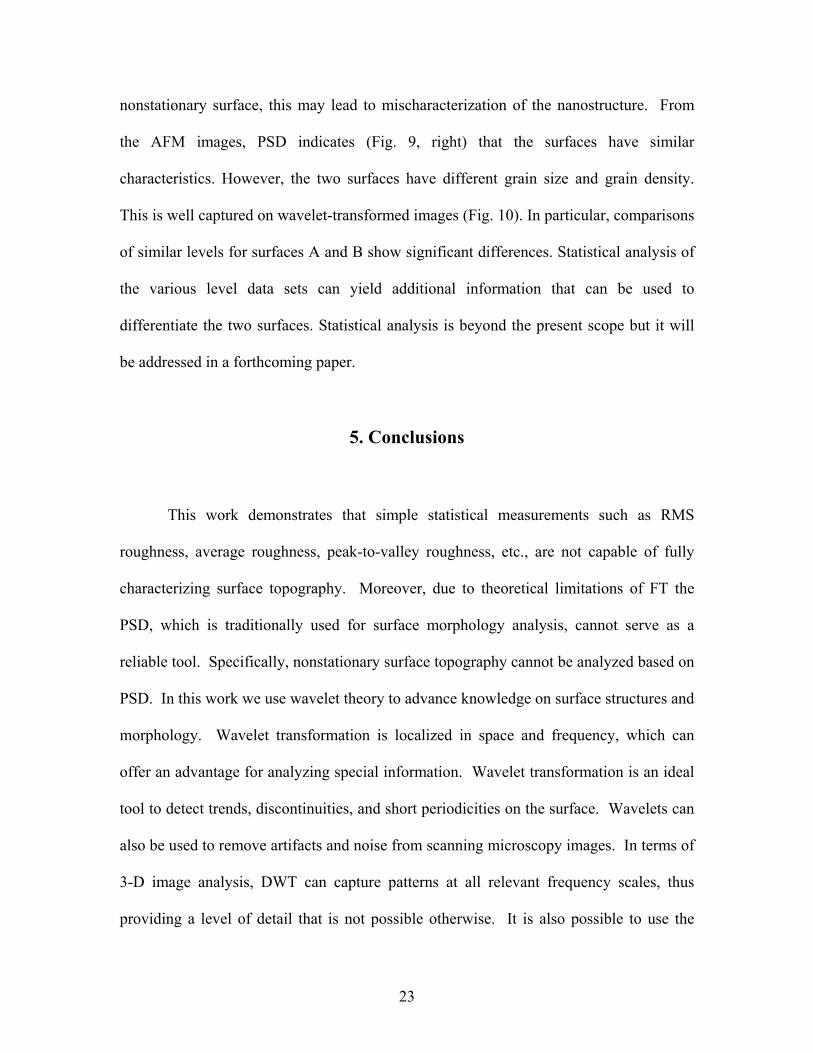
An example of a non-uniform surface pattern is shown in Figure 7a. The surface is

characterized by a large-size grain-like aggregate in the middle of a surface of uniform

grain morphology. The AFM image is clear in both force and height modes, which

permits straightforward topographic surface measurements. However, due to the non-

19

stationary nature of this surface (where different frequency components appear for a short

range), topographic surface measurements based on standard methods such as RMS

roughness, PSD or other traditional techniques would not accurately characterize the

surface. Therefore, we can make use of DWT obtained by a multiresolution scheme that

allows the signal to be decomposed into different frequency components through a set of

low-pass and high-pass filters at desired decomposition level. These components can

then be used to analyze surface features at different decomposition levels and, if

necessary, to reconstruct the original image. After DWT decomposition of a 3D image,

we can get multiple images of detailed coefficients and final approximation coefficients

(Fig. 7b). Approximation coefficients usually represent the base structure of the surface,

since the high frequency components are removed. Consequently, the study of the

approximation coefficients allows us to capture the surface inhomogeneity and analyze it

in much greater detail. In other words, this method allows us to separate the surface

details by filtering at different scales and identify the exact location of the surface

inhomogeneities. Analysis at each level of detail (from small to large) separately on the

same image is now possible. Figure 7b also shows in Level 5 details of a periodic surface

structure, which is not detected in the original AFM image. The observed periodicity,

which is characteristic for the whole image, also suggests that the agglomeration has in

fact the same structure (possible the same composition) as the background.

In this particular case of non-uniform surface patterns, it is important to separate low

frequency components, which usually represent the base structure of the surface, from its

high frequency components and perform measurements on wavelet-reconstructed image

with high frequency components only. This procedure, for example, can also be effective

20

to analyze the kinetics of thin film deposition using the in situ AFM techniques.

Additionally, nanoscale features can be further quantified and can be used to monitor the

evolution of film deposition at specific frequency scales. The advantage of this approach

is that it offers simultaneous structural and kinetics data on thin films that can be used for

modeling purposes.

These preliminary results demonstrate superior capabilities of wavelet approach to

microscopic image analysis over traditional techniques. It is also possible to use this

methodology for analyzing surface structures at the molecular level [21-23].

4.2 Removing AFM artifacts and noise from images

Unlike inorganic surfaces, which are hard surfaces, organic layers have inherent

visualization problems related to the quality of the AFM image due to the wet

environment required for imaging organic layers, and to the softness and mobility of the

surface layer. AFM can image a surface either by maintaining a constant (contact mode)

or intermittent (tapping mode) contact of the scanning tip with the sample, depending on

the particularities of a given surface. However, AFM images may contain artifacts,

distortion and noise due to corrupted scanning features. These artifacts may also be

caused by other sources such as vibration of the cantilever, an unstable and/or moving

surface, random noise, or other causes related to imaging conditions. Wavelet Transform

can help identify such artifacts and noise and in some cases remove them from AFM

images.

21

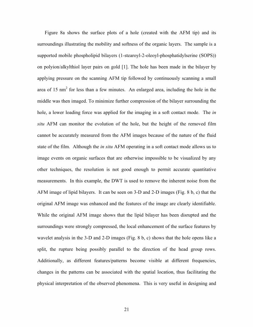
Figure 8a shows the surface plots of a hole (created with the AFM tip) and its

surroundings illustrating the mobility and softness of the organic layers. The sample is a

supported mobile phospholipid bilayers (1-stearoyl-2-oleoyl-phosphatidylserine (SOPS))

on polyion/alkylthiol layer pairs on gold [1]. The hole has been made in the bilayer by

applying pressure on the scanning AFM tip followed by continuously scanning a small

area of 15 nm2 for less than a few minutes. An enlarged area, including the hole in the

middle was then imaged. To minimize further compression of the bilayer surrounding the

hole, a lower loading force was applied for the imaging in a soft contact mode. The in

situ AFM can monitor the evolution of the hole, but the height of the removed film

cannot be accurately measured from the AFM images because of the nature of the fluid

state of the film. Although the in situ AFM operating in a soft contact mode allows us to

image events on organic surfaces that are otherwise impossible to be visualized by any

other techniques, the resolution is not good enough to permit accurate quantitative

measurements. In this example, the DWT is used to remove the inherent noise from the

AFM image of lipid bilayers. It can be seen on 3-D and 2-D images (Fig. 8 b, c) that the

original AFM image was enhanced and the features of the image are clearly identifiable.

While the original AFM image shows that the lipid bilayer has been disrupted and the

surroundings were strongly compressed, the local enhancement of the surface features by

wavelet analysis in the 3-D and 2-D images (Fig. 8 b, c) shows that the hole opens like a

split, the rupture being possibly parallel to the direction of the head group rows.

Additionally, as different features/patterns become visible at different frequencies,

changes in the patterns can be associated with the spatial location, thus facilitating the

physical interpretation of the observed phenomena. This is very useful in designing and

22

engineering nanostructures, studying complex interactions, their mechanism and kinetics

by using high-resolution SPMs.

4.3 Characterization of surface topography

This example shows two different substrates with similar topography but different

composition and processing conditions. This is a common application in thin film

technology. One of the major concerns in thin film deposition is the reduction of surface

and interface roughness. This is because the surface structure of thin films critically

affects the performance of nanoscale devices. The interest in searching for new methods

to characterize surface roughness resides in understanding of surface roughness

measurements down to atomic scale. This approach allows us to have control over the

deposition process, i.e. to optimize the film-processing route and to control the changes in

surface roughness with the film growth and processing conditions.

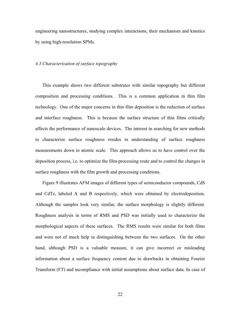
Figure 9 illustrates AFM images of different types of semiconductor compounds, CdS

and CdTe, labeled A and B respectively, which were obtained by electrodeposition.

Although the samples look very similar, the surface morphology is slightly different.

Roughness analysis in terms of RMS and PSD was initially used to characterize the

morphological aspects of these surfaces. The RMS results were similar for both films

and were not of much help in distinguishing between the two surfaces. On the other

hand, although PSD is a valuable measure, it can give incorrect or misleading

information about a surface frequency content due to drawbacks in obtaining Fourier

Transform (FT) and incompliance with initial assumptions about surface data. In case of

23

nonstationary surface, this may lead to mischaracterization of the nanostructure. From

the AFM images, PSD indicates (Fig. 9, right) that the surfaces have similar

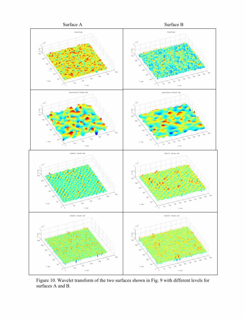
characteristics. However, the two surfaces have different grain size and grain density.

This is well captured on wavelet-transformed images (Fig. 10). In particular, comparisons

of similar levels for surfaces A and B show significant differences. Statistical analysis of

the various level data sets can yield additional information that can be used to

differentiate the two surfaces. Statistical analysis is beyond the present scope but it will

be addressed in a forthcoming paper.

5. Conclusions

This work demonstrates that simple statistical measurements such as RMS

roughness, average roughness, peak-to-valley roughness, etc., are not capable of fully

characterizing surface topography. Moreover, due to theoretical limitations of FT the

PSD, which is traditionally used for surface morphology analysis, cannot serve as a

reliable tool. Specifically, nonstationary surface topography cannot be analyzed based on

PSD. In this work we use wavelet theory to advance knowledge on surface structures and

morphology. Wavelet transformation is localized in space and frequency, which can

offer an advantage for analyzing special information. Wavelet transformation is an ideal

tool to detect trends, discontinuities, and short periodicities on the surface. Wavelets can

also be used to remove artifacts and noise from scanning microscopy images. In terms of

3-D image analysis, DWT can capture patterns at all relevant frequency scales, thus

providing a level of detail that is not possible otherwise. It is also possible to use the

24

methodology for analyzing surface structures at the molecular level. The results

demonstrate superior capabilities of wavelet approach to microscopic image analysis over

traditional techniques.

References

1. L. Zhang, R. Vidu, A. J. Waring, R. I. Lehrer, M. L. Longo, and P. Stroeve,Langmuir 18:1318 (2002).

2. R. Vidu, L. Zang, A. J. Waring, M. L. Longo, and P. Stroeve, Material Scienceand Engineering B 96:199 (2002).

3. R. Vidu, T. Ratto, M. Longo, and P. Stroeve, in Planar Lipid Bilayers (BLMs) andtheir Applications (H. T. Tien, ed.), Elsevier, 2003, p. 886.

4. A. A. Levchenko, B. P. Argo, R. Vidu, R. V. Talroze, and P. Stroeve, Langmuir18:8464 (2002).

5. F. T. Quinlan, K. Sano, T. Willey, R. Vidu, K. Tasaki, and P. Stroeve, Chemistryof Materials 13:4207 (2001).

6. J. M. Bennett and L. Mattsson, Introduction to surface roughness and scattering,Optical Society of America, Washington, D.C., 1989.

7. S. J. Fang, S. Haplepete, W. Chen, C. R. Helms, and H. Edwards, Journal ofApplied Physics 82:5891 (1997).

8. A. Duparre, J. Ferre-Borrull, S. Gliech, G. Notni, J. Steinert, and J. M. Bennett,Applied Optics 41:154 (2002).

9. S. M. Kay, Modern spectral estimation : theory and application, Prentice Hall,Englewood Cliffs, N.J., 1988.

10. L. Angrisani, L. Bechou, D. Dallet, P. Daponte, and Y. Ousten, Measurement31:77 (2002).

11. B. K. Alsberg, A. M. Woodward, and D. B. Kell, Chemometrics & IntelligentLaboratory Systems 37:215 (1997).

12. P. M. Bentley and J. T. E. McDonnell, Electronics & CommunicationEngineering Journal 6:175 (1994).

13. A. Graps, IEEE Computational Science & Engineering 2:50 (1995).14. O. Rioul and M. Vetterli, IEEE SP Magazine 8:14 (1991).15. A. A. Petrosian and F. G. Meyer, Wavelets in signal and image analysis ; from

theory to practice, Kluwer Academic, Dordrecht ; Boston, 2001.

25

16. S. M. Kay, Modern Spectral Estimation, Prentice Hall, 1988, NJ, 1988.

17. S. Qian, Introduction to time-frequency and wavelet transforms, Prentice HallPTR, Upper Saddle River, N.J., 2002.

18. R. N. Bracewell, The Fourier Transform and its Application, McGraw-Hill, NewYork, NY, 1986.

19. S. G. Mallat, IEEE Trans. Pattern Anal. Machine Intell. 11:674 (1989).20. F. Doymaz, A. Bakhtazad, J. A. Romagnoli, and A. Palazoglu, Computers &

Chemical Engineering 25:1549 (2001).21. Z. Moktadir and K. Sato, Surface Science 470:L57 (2000).22. F. El Feninat, S. Elouatik, T. H. Ellis, E. Sacher, and I. Stangel, Applied Surface

Science 183:205 (2001).23. N. Bonnet and P. Vautrot, Microscopy Microanalysis Microstructures 8:59

(1997).

Figure 1. Example of two surface roughness profiles compared to the normal distributioncurve: (a) isotropic surface and its distribution bar chart; (b) non-isotropic surface with

bumps and holes and its distribution bar chart.

(b)

RMS Ra

(a)

RMS Ra

Figure 2. Fourier transform of two artificial surface profiles: (a) is a sum of three sinewaves with 10, 50, and 100 Hz frequencies and white noise; (b) is composed of three sine

waves with 10, 50, and 100 Hz frequencies, at different lengths, and white noise.

(a)

(b)

Figure 3. PSD function of two artificial surface profiles: (a) PSD spectrum of a profilecomposed of 3 sine waves at different frequencies (5, 25 and 50 Hz); (b) PSD spectrum

of a profile composed of 3 sine waves at different frequencies (15, 30 and 45 Hz).

(a)

(b)

Figure 4. Commonly used Wavelets: (a) Haar, (b) Daubechies 2, (c) Symlet 10, and (d)Morlet 16.

(a) (b)

(c) (d)

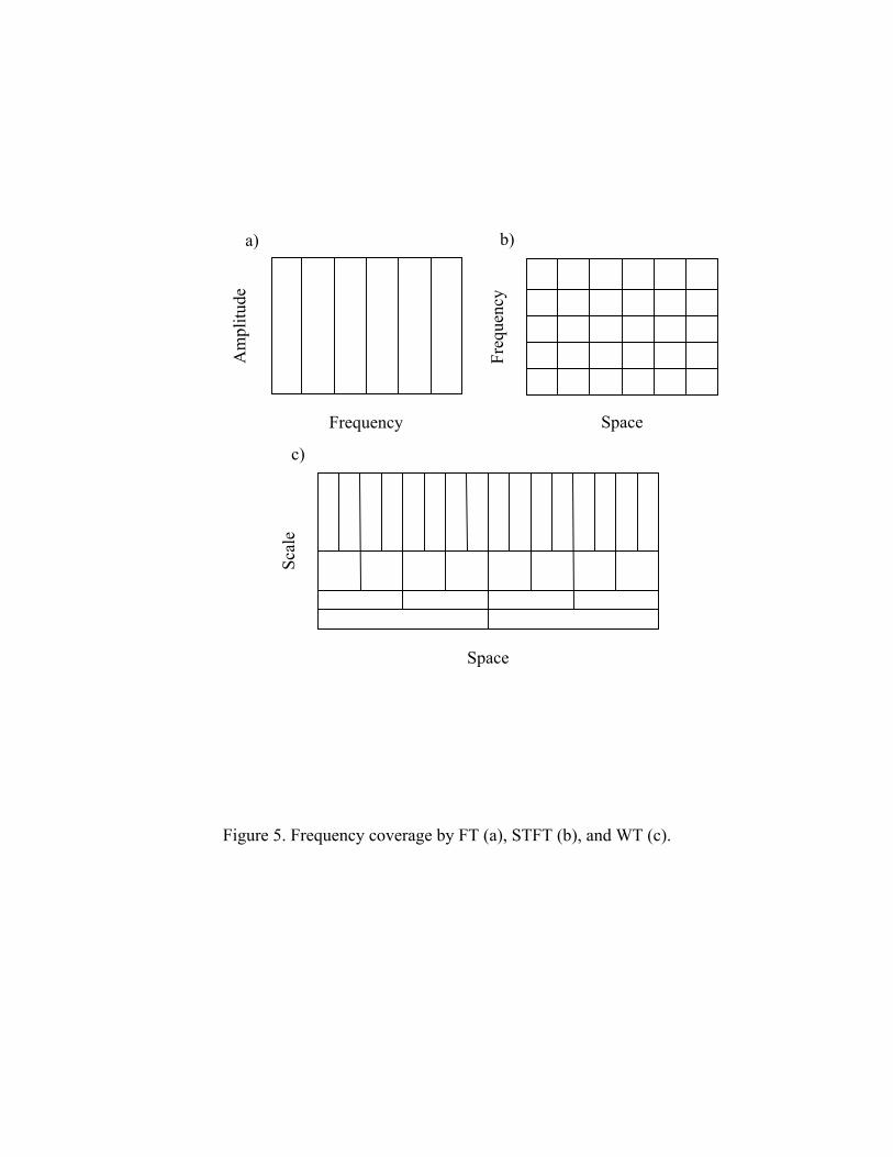
Figure 5. Frequency coverage by FT (a), STFT (b), and WT (c).

c)

b)a)

Space

Freq

uenc

y

Space

Am

plitu

de

Scal

e

Frequency

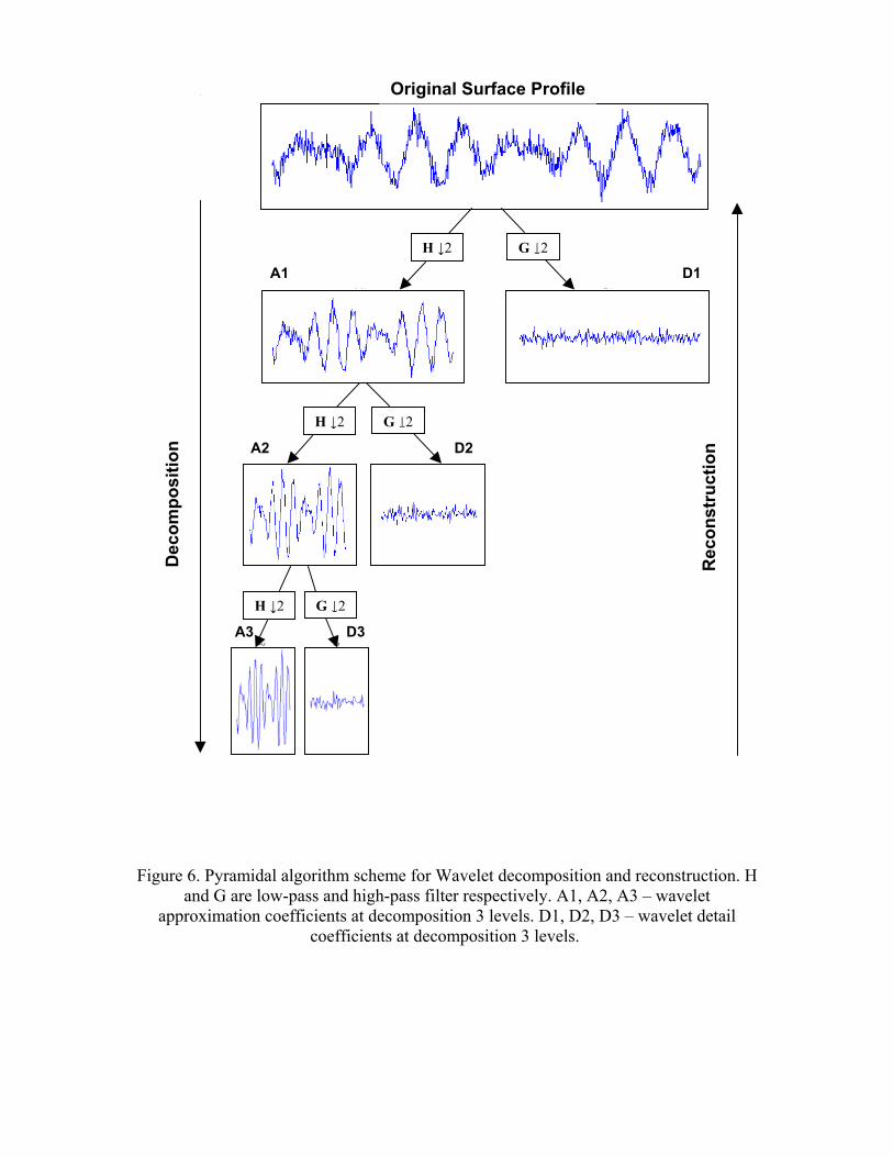
Figure 6. Pyramidal algorithm scheme for Wavelet decomposition and reconstruction. Hand G are low-pass and high-pass filter respectively. A1, A2, A3 – wavelet

approximation coefficients at decomposition 3 levels. D1, D2, D3 – wavelet detailcoefficients at decomposition 3 levels.

Original Surface Profile

H ↓2 G ↓2

A1 D1

A2 D2

H ↓2 G ↓2

A3 D3

H ↓2 G ↓2

Dec

ompo

sitio

n

Rec

onst

ruct

ion

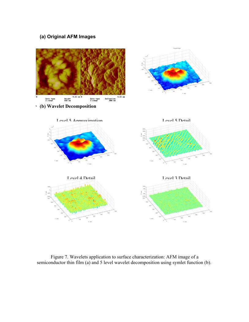
Figure 7. Wavelets application to surface characterization: AFM image of asemiconductor thin film (a) and 5 level wavelet decomposition using symlet function (b).

(a) Original AFM Images

Level 5 Approximation Level 5 Detail

Level 4 Detail Level 3 Detail

(b) Wavelet Decomposition

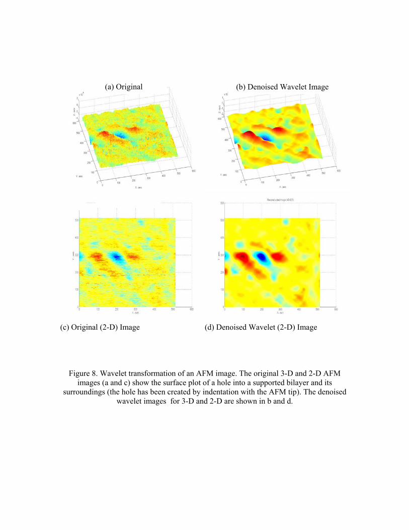
(c) Original (2-D) Image (d) Deno

Figure 8. Wavelet transformation of an AFM imageimages (a and c) show the surface plot of a hole i

surroundings (the hole has been created by indentatiowavelet images for 3-D and 2-D are

(b)

(a) Original (b) Denoised Wavelet Image

Wavelet Denoised Image

ised Wavelet (2-D) Image

. The original 3-D and 2-D AFMnto a supported bilayer and itsn with the AFM tip). The denoised shown in b and d.

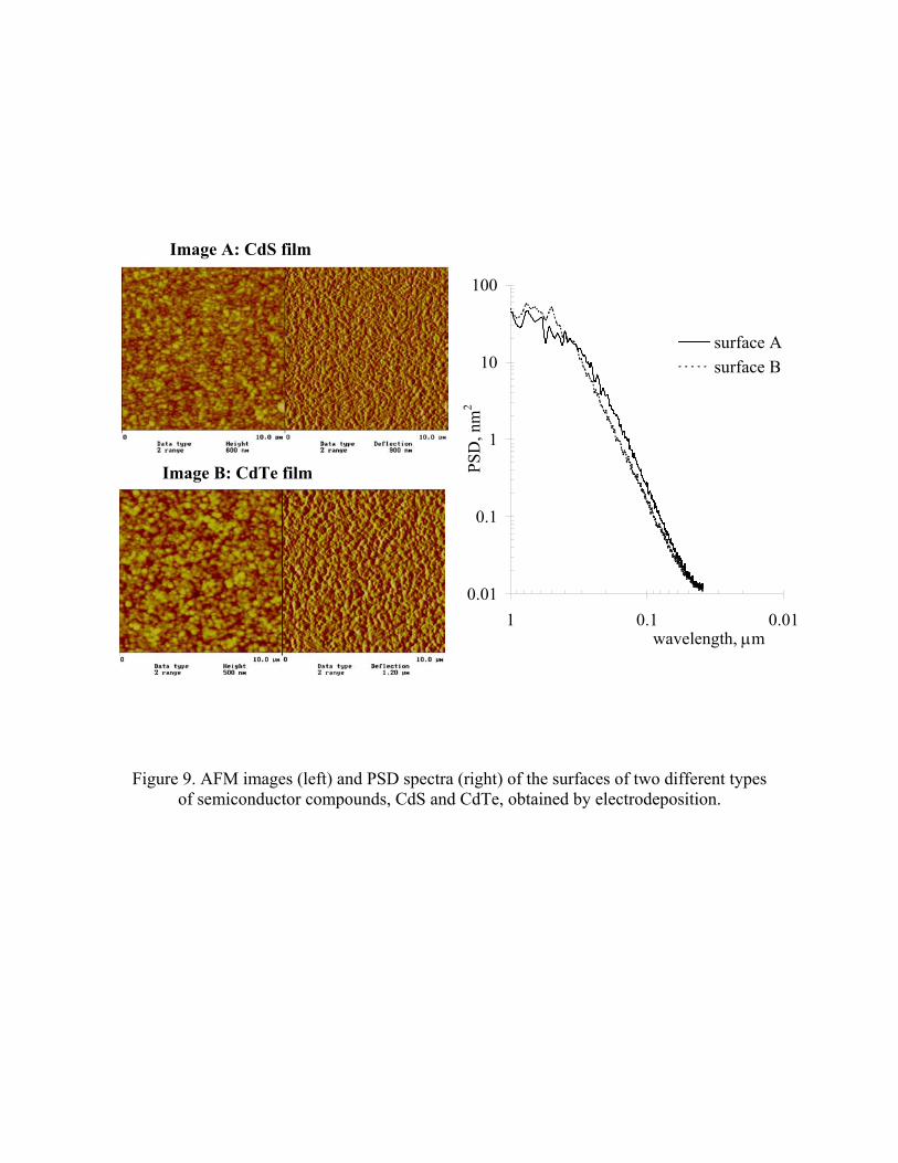
Figure 9. AFM images (left) and PSD spectra (right) of the surfaces of two different typesof semiconductor compounds, CdS and CdTe, obtained by electrodeposition.

Image A: CdS film

0.01

0.1

1

10

100

0.010.11wavelength, µm

PSD

, nm

2

surface Asurface B

Image B: CdTe film

Surface A Surface B

Figure 10. Wavelet transform of the two surfaces shown in Fig. 9 with different levels forsurfaces A and B.