Entropy from Correlations in TIP4P Water

Emanuela Giuffre,1, ∗ Santi Prestipino,1, †

Franz Saija,2, ‡ A. Marco Saitta,3, § and Paolo V. Giaquinta1, ¶

1Universita degli Studi di Messina, Dipartimento di Fisica,

Contrada Papardo, 98166 Messina, Italy

2CNR - Istituto per i Processi Chimico-Fisici,

Sede di Messina, Contrada Papardo,

Viale Ferdinando Stagno d’Alcontres 37, 98158 Messina, Italy

3Universite Pierre et Marie Curie – Paris 06,

UMR 7590, IMPMC, F-75015 Paris, France

(Dated: February 3, 2010)

Abstract

We use Molecular Dynamics to compute the pair distribution function of liquid TIP4P water

as a function of the intermolecular distance and of the five angles that are needed to specify

the relative position and orientation of two water molecules. We also calculate the translational

and orientational contributions to the two-body term in the multiparticle correlation expansion

of the configurational entropy at three selected thermodynamic states, where we also test various

approximations for the angular dependence of the pair distribution function. We finally compare

the results obtained for the pair entropy of TIP4P water with the experimental values of the excess

entropy of ordinary water.

PACS numbers: 05.20.Jj, 61.20.Ja, 64.10.+h

Keywords: Molecular liquids; water; TIP4P; pair entropy; excess entropy; orientational correlations.

1

I. INTRODUCTION

It is superfluous to motivate the persisting interest in a deeper understanding and more

effective modeling of the equilibrium structure of water.1 The paradigmatic status of this

molecular liquid in the realms of natural and life sciences, at the interface between a variety

of disciplines such as physics, chemistry, and biology, justifies the continuing efforts that are

being made to refine experimental tools and theoretical approximations so as to achieve more

and more reliable predictions of the microscopic and macroscopic properties of this substance

as well as of the many anomalous aspects that mark its thermodynamical, structural, and

dynamical behavior in a unique way.2

The main object of the present study is the calculation of the pair entropy of liquid water,

i.e., the contribution of two-body density correlations to the configurational entropy. The

statistical-mechanical framework is that provided by the multiparticle correlation expansion

of the excess entropy, originally derived for a classical atomic fluid in the canonical ensem-

ble3,4 and later extended to the grand-canonical ensemble,5,6 the two expressions having in

fact been shown to be formally equivalent.7 Many other authors have discussed this topic;

we refer the reader to Ref. 8 for a short commented list of some relevant contributions to

the subject. To our knowledge, the first calculation of the pair entropy of a pure molecular

fluid dates back to the seminal paper authored by Lazaridis and Karplus,9 who investigated

the interplay between orientational correlations and entropy in the TIP4P model of liquid

water.10 The TIP4P potential is an effective pairwise four-site potential: a Lennard-Jones

interaction site is located on the oxygen, two positive charges on the hydrogens and an

extra negative charge is located away from the oxygen along the hydrogen-hydrogen bisec-

tor. Intramolecular degrees of freedom are neglected in the TIP4P model but, nonetheless,

this potential turns out to be a good transferable potential in that it ultimately provides a

qualitatively correct representation of the phase diagram of water, also in comparison with

other interaction models, except at very high pressure.11,12

The calculation of the pair entropy for a given model potential requires the knowledge

of the pair distribution function (PDF) of the molecular liquid, a quantity that, in the case

of TIP4P water, depends on six variables, viz., the distance between the centers of mass of

the two molecules and five angles that are needed to specify their relative orientation. Such

a function cannot be easily obtained from numerical simulation since a statistically reliable

2

result requires a massive numerical sampling to be carried out over a discrete six-dimensional

grid whose spacing is consequently the outcome of a delicate compromise between the avail-

able computer power and the desired quantitative accuracy of the calculation. This is

precisely the reason why Lazaridis and Karplus evaluated the pair entropy of liquid TIP4P

water using a variety of approximations for the five-dimensional orientational distribution

function (ODF) which, computed at a given intermolecular separation and then multiplied

by the ordinary radial distribution function (RDF), eventually yields the full six-dimensional

PDF. Such approximations implemented partial representations of the ODF based on com-

binations of the monovariate and bivariate angular distribution functions as obtained from

numerical simulation.

A few other attempts have as yet followed the route traced by Lazaridis and Karplus for

the calculation of the pair entropy of water. Giaquinta and coworkers exploited one of the

approximate schemes illustrated in Ref. 9 the so-called “adjusted gas-phase” (AGP) approxi-

mation, to highlight different ordering regimes in liquid TIP4P water13 and to “measure” the

relative amounts of positional and angular order through the translational and orientational

pair entropies, used for the first time together as unbiased, self-consistent, and independent

“order parameters” to map the phase diagram of water.14 The first “exact” calculation – i.e.,

one performed without resorting to any approximate partial representation of the ODF – of

the pair entropy was carried out by Zielkiewcz in four different models of computer water

at ambient conditions.15,16 A temperature analysis of the results for the single-point charge

(SPC) model was later presented by the same author.17 More recently, Wang and coworkers

suggested a novel nonparametric approach to computing the pair entropy, alternative to

the histogram-based method, and further based on a generalized Kirkwood superposition

approximation (GKSA) for the ODF.18 This approach was tested in five water models at

ambient conditions.

In this paper we present the results of a numeric calculation of the full PDF of liq-

uid TIP4P water, carried out with the method of Molecular Dynamics (MD), at ambient

conditions as well as in two other thermodynamic states, at lower temperature and higher

pressure, respectively. The general theoretical framework is introduced and discussed in

Sec. II, together with the approximations that were implemented for the ODF in addition to

the direct MD calculations, whose technical details are summarized in Sec. III. The resulting

translational and orientational pair entropies are presented in Sec. IV and therein compared

3

with the experimental data for the excess entropy of ordinary water. Section V is finally

devoted to concluding remarks.

II. THEORETICAL FRAMEWORK

A. Pair entropy of a molecular liquid

Statistical mechanics provides a general expression for the entropy of a classical, atomic

or molecular, fluid which, in general, can be written as an infinite sum of contributions

associated with spatially integrated n-point density correlations:

Sex =∞∑n=2

Sn , (1)

where Sex is the excess (with respect to the corresponding ideal gas) entropy. In the ab-

sence of external fields, the two-body term – that, in the following, we shall refer to as the

“pair entropy” – ordinarily delivers the dominant contribution to the excess entropy of a

liquid.13,19,20 As such, S2 has been often used as an approximate “local” (in thermodynamic

space) estimate of Sex in that the calculation of the pair entropy does not require a ther-

modynamic potential to be integrated along an extended path connecting the state whose

entropy one is interested in with another (reference) state where the thermodynamic prop-

erties of the fluid are known by independent means, as in the high-temperature ideal-gas

asymptotic regime, or can be computed with other techniques.12,21

The pair entropy of molecular fluids reads:9,22

S2 = −1

2kB

( ρΩ

)2 ∫[g(r1, r2, ξ1, ξ2) ln g(r1, r2, ξ1, ξ2)− g(r1, r2, ξ1, ξ2) + 1] dr1 dr2 dξ1 dξ2 ,

(2)

where kB is the Boltzmann constant, ρ is the particle number density, and g(r1, r2, ξ1, ξ2)

is the PDF which, in general, depends on the vector radii (r1, r2) of the molecular centers

of mass and on the pair of Euler angles sets (ξ1, ξ2), where ξα ≡ θα, φα, χα specifies

the absolute orientation of the αth molecule in the laboratory reference frame x, y, z.

The three Euler angles are respectively defined in the ranges 0 ≤ θα ≤ π, 0 ≤ φα < 2π,

and 0 ≤ χα < 2π, with angular elements dξα = sin(θα) dθα dφα dχα. Correspondingly,

Ω ≡∫

dξα = 8π2. We note that the set of variables introduced above is in fact redundant

for a homogeneous and isotropic molecular fluid since, in the absence of external fields,

4

the PDF depends on the relative position and orientation of the two molecules. For water

molecules this information can be encoded into six variables only, viz., the radial separation

r between the centers of mass plus five angles. In fact, let us label the oxygen and hydrogen

atoms of the αth molecule as Oα, H1α, and H2α, respectively; let us further identify the

mean point of the segment H1αH2α, joining the two hydrogen atoms, as Dα. In terms of the

unit vectors

z =

−−−→O1O2

|−−−→O1O2|

, zα =

−−−→OαDα

|−−−→OαDα|

, (3)

one has for the angle θα formed by the dipole moment of the αth molecule, lying in the

direction zα, and the intermolecular axis z:

θα = arccos (zα · z) (0 ≤ θα ≤ π) . (4)

In order to define the other Euler angles, we need to specify a reference system xα, yα, zα

sticking out of each molecule. This can be done by defining, for instance, the xα and yα

axes as

xα =

−−−−−→H2αH1α

|−−−−−→H2αH1α|

, yα = zα ∧ xα . (5)

Hence, in terms of the auxiliary unit vector

Nα ≡z ∧ zα|z ∧ zα|

, (6)

specifying the line of nodes that is associated with the αth molecule, we obtain:

φα = arg(x · Nα, y · Nα

)(0 ≤ φα ≤ 2π) (7)

and

χα = arg(xα · Nα,−yα · Nα

)(0 ≤ χα ≤ 2π) , (8)

where arg(u, v) is the polar argument of the vector (u, v). The angle χα describes the

rotation of the αth water molecule around its own dipole vector. One can readily see that

one of the above six angles is superfluous; in fact, upon choosing, say, x ≡ N1, the angle

φ1 identically vanishes. In the following, we shall refer to this set of angular coordinates as

the A set. Actually, one may further take advantage of a symmetry of the PDF that follows

from the observation that the pointing directions of the unit vectors x1 and x2 depend on

the (arbitrary) way one has labeled the two hydrogen atoms within each water molecule.

In turn, this choice uniquely determines the pointing directions of y1 and y2. This residual

5

freedom reflects on the behavior of the (exact) PDF that is in fact invariant under χα

rotations moving this angle to [χα + π (mod 2π)]. Hence, it should suffice to consider the

dependence of the PDF on χα within the interval [0, π]. We shall refer to this modified – by

effect of symmetry – set of variables as the As set.

The above choice of variables closely recalls the one made by Lazaridis and Karplus.9

However, in addition to the pairs (θ1, θ2) and (χ1, χ2), they used the angle φ ≡ φ1 − φ2 de-

scribing the relative rotation of a pair of molecules (more specifically, of their respective

line-of-nodes unit vectors, N1 and N2) around the intermolecular axis. Moreover, their

conventions on how to measure the two pairs of angles mentioned above differ from those

specified for the set A. In particular, H11 was explicitly taken to be the hydrogen atom of

molecule 1 that is closest to the oxygen atom of molecule 2, and similarly for H21 (see Fig. 1

of Ref. 9 and the relative caption). Lazaridis and Karplus further exploited a number of

symmetries of the PDF involving all the five angles. In fact, in addition to those introduced

above which concern the pairs (θ1, θ2) and (χ1, χ2), they also considered two residual sym-

metries of the PDF: they noted that the two water molecules are interchangeable, which

allows one to integrate the angle θ2 from θ1 to π, and also observed that the the angle φ

can be integrated from 0 to π only. We shall refer to this set of angular coordinates as the

Bs set which, however, we shall implement without resorting to the additional symmetry

concerning the angle θ2.

A still different choice (C) was made by Zielkiewicz15,16 who assumed x, y, z ≡

x1, y1, z1, the orthonormal triad attached to molecule 1 being specified as above by Eqs. (3)

and (5). He then considered the spherical coordinates of O2 in the reference frame centered

on O1:

Θ = arccos (r · z1) , Φ = arg (x1 · r⊥, y1 · r⊥) , (9)

where r ≡−−−→O1O2, r⊥ = r − (r · z1) z1, with 0 ≤ Θ ≤ π and 0 ≤ Φ ≤ 2π, in addition to

the three Euler angles (θ2, φ2, χ2) that specify the global orientation of the second molecule

with respect to the central one, according to Eqs. (4), (7), and (8). As observed before, the

alternative for xα is twofold, allowing one to restrict the range of φ2 and χ2 to the interval

[0, π]. The set of variables where this latter symmetry property is employed will be referred

to as the Cs set.

It is important to realize that different choices of the angles that specify the relative

orientation of two water molecules, as well as of the associated intervals within which the

6

PDF is then being sampled, lead to different histograms and, consequently, to potentially

different numerical estimates of the pair entropy. This is obviously due to the finite integra-

tion meshes as well as to the number of symmetries that are implemented in each angular

set. In fact, we should expect that the best results will be achieved when one makes full

use of the symmetries of the PDF which is actually the case of the Bs set. In this respect,

we note that, for an assigned number of configurations over which the PDF histogram is

being sampled, the information contents of the histograms built by using the As and Cs sets

should be four times larger than that of the corresponding histograms in the A and C sets.

On the other hand, the statistical quality achieved with the Bs set should be twice as better

as that achieved with the As and Cs sets.

Now, let Ψ be any fivefold set of independent angular variables. Upon observing that∫dξ1dξ2 = 2π

∫dΨ, we can rewrite Eq. (2) as

s2 = −kB(

2π

Ω

)2

ρ

∫[g(r,Ψ) ln g(r,Ψ)− g(r,Ψ) + 1] r2dr dΨ , (10)

where s2 is the pair entropy per particle. Following Lazaridis and Karplus,9 we factorize the

PDF as

g(r,Ψ) = g(r)g(Ψ|r) , (11)

where g(r) is the RDF and g(Ψ|r) is the conditional distribution for the relative orientation

of two molecules separated by a distance r, i.e., the quantity that we shall refer to in the

following as the ODF. The following normalization condition holds:

2π

Ω2

∫g(r,Ψ)dΨ = g(r) . (12)

Correspondingly, the pair entropy can be resolved into the sum of two terms:

s2 = s(tr)2 + s

(or)2 (13)

where

s(tr)2 = −kB(2π)ρ

∫ ∞0

[g(r) ln g(r)− g(r) + 1] r2dr (14)

is the translational pair entropy and

s(or)2 =

∫ ∞0

ρ g(r)S(or)(r) r2dr (15)

7

is the orientational pair entropy that is defined in terms of the orientational local entropy

(OLE):

S(or)(r) = −kB(

2π

Ω

)2 ∫g(Ψ|r) ln g(Ψ|r)dΨ. (16)

B. Approximations for the pair distribution function

At variance with the RDF, the numerical evaluation of the ODF is a formidable compu-

tational task because of the number of variables this function depends on. Approximating

the ODF may be in many cases the only viable route to the calculation of the orientational

contribution to the thermodynamic properties of liquid water. In this respect, Lazaridis and

Karplus proposed a number of approximate schemes for the full PDF, essentially based on

the assumption that the ODFs of gaseous and liquid water have similar short range struc-

tures.9 The first “family” of such approximations was generated by factorizing the ODF

into a product of one-dimensional (1d) and two-dimensional (2d) marginals, defined as the

probability distributions of one angle, or the joint probability distributions of two angles,

regardless of the values attained by the remaining angles:

g(Ψi|r) ≡∫g(Ψ|r)d4Ψj 6=i∫

d4Ψj 6=i, (17)

and

g(Ψi,Ψj|r) ≡∫g(Ψ|r)d3Ψk 6=i,j∫

d3Ψk 6=i,j. (18)

Lazaridis and Karplus (LK) introduced and discussed various factorizations that were tested

against the thermodynamic properties (energy, entropy) of the gas phase of TIP4P water.9

They eventually concluded that, overall, the most balanced scheme was the one which they

referred to as the F7 factorization:

g(F7)LK (θ1, θ2, φ, χ1, χ2) ≡

[g(θ1, θ2)g(χ1, χ2)g(θ1, χ2)g(θ2, χ1)

g(θ1)g(θ2)g(χ1)g(χ2)

]g(φ) , (19)

where the parametric dependence on the radial separation r is implicit in both the full and

marginal ODFs that appear on the left and right hand side of Eq. (19), respectively. This

approximation exploits the “flatness” of the ODF with respect to the angle φ and the ensuing

absence, in the liquid phase, of significant correlations between φ and the other angles.9

In addition to the factorization scheme illustrated above, Lazaridis and Karplus described

a different approach based on the low-density limit of the ODF, modified by a subset of the

8

marginal ODFs that were obtained from the numerical simulations of liquid TIP4P water.

The resulting AGP approximation for the ODF can be written as follows:

g(AGP)LK (θ1, θ2, φ, χ1, χ2) = gs(θ1, θ2, φ, χ1, χ2) · CLK(θ1, θ2, φ, χ1, χ2) (20)

where

CLK(θ1, θ2, φ, χ1, χ2) =g(θ1, θ2)

gs(θ1, θ2)· g(χ1, χ2)

gs(χ1, χ2)· g(φ)

gs(φ), (21)

and where we have again suppressed the dependence on the intermolecular distance r. In

Eq. (21) g(θ1, θ2), g(χ1, χ2), and g(φ) are the “exact” marginals, which can be calculated by

numerical simulation, while the function gs and the associated marginals follow from

gs(Ψ|r) ≡ ggas(Ψ|r) + S (r) [1− ggas(Ψ|r)] , (22)

where

ggas(Ψ|r) =

(Ω2

2π

)exp[−βu(r,Ψ)]∫

exp[−βu(r,Ψ)]dΨ, (23)

u(r,Ψ) being the interaction potential and

S (r) =UMD(r)− Ugas(r)

U(r)− Ugas(r). (24)

In Eq. (24) UMD(r) is the angularly averaged interaction energy evaluated at a specified

distance r through the MD simulation, Ugas(r) is the corresponding quantity calculated in

the gas phase, and U(r) is the unweighted average of u(r,Ψ) over orientations. The ODF

that follows from Eq. (20) must be eventually normalized so as to satisfy Eq. (12). The

smoothing function S (r) is such that the angularly averaged energy evaluated through the

function gs reproduces the quantity UMD(r).

As seen from Eqs. (20) and (21), the naive gas-phase approximation – formulated in

Eqs. (22), (23), and (24) – is adjusted so as to enforce, through the CLK factor, a reasonable

degree of consistency between the resulting ODF and a subset of liquid-phase marginal

distributions. Wang and coworkers18 recently noted that a non-negligible correlation exists

between the angles θ and χ of each water molecule which cannot be accounted for by the

mere product of the corresponding 1d marginals, i.e., g(θ) and g(χ). Hence, they proposed

a GKSA factorization of the ODF that differs from the F7 scheme set up by Lazaridis and

Karplus in that the modified ODF includes an extra pair of 2d “intramolecular” marginals,

viz., g(θ1, χ1) and g(θ2, χ2). Motivated by this observation, we also report in this paper

9

on three variants of the original AGP approximation where the coupling factor CLK, which

appears in Eq. (20), has been replaced, in turn, by the following expressions:

C1(θ1, θ2, φ, χ1, χ2) = CLK(θ1, θ2, φ, χ1, χ2)

[g(θ1, χ1)

gs(θ1, χ1)· g(θ2, χ2)

gs(θ2, χ2)

], (25)

C2(θ1, θ2, φ, χ1, χ2) = CLK(θ1, θ2, φ, χ1, χ2)

[g(θ1, χ2)

gs(θ1, χ2)· g(θ2, χ1)

gs(θ2, χ1)

], (26)

C3(θ1, θ2, φ, χ1, χ2) = C2(θ1, θ2, φ, χ1, χ2)

[g(θ1, χ1)

gs(θ1, χ1)· g(θ2, χ2)

gs(θ2, χ2)

]. (27)

We shall refer to the three modified AGP schemes reported in Eqs. (25), (26), and (27)

as the AGP1, AGP2, and AGP3 approximation, respectively. We observe that the AGP2

approximation includes the same 2d marginals that also appear in the F7 approximation

originally proposed by Lazaridis and Karplus,9 while the AGP3 coupling factor reproduces

the factorization of 2d marginals adopted by Wang and coworkers.18

In order to simplify the calculation of the pair entropy, Lazaridis and Karplus further

resorted to an approximate computational strategy. In fact, they averaged the liquid-phase

angular distributions that appear in both the F7 and AGP schemes over three distinct spa-

tial regions (“shells”) whose boundaries were chosen so as to coincide with the positions of

the first peak and of the first two troughs in the oxygen-oxygen RDF of TIP4P water at

25 C and 1 atm. Their choice leads to the following intervals: 0 ≤ r ≤ 0.28 nm, 0.28 nm <

r ≤ 0.34 nm, and 0.34 nm < r ≤ 0.56 nm. As for the three gas-phase marginals that also

contribute to the AGP approximation, they were apparently calculated at three “represen-

tative” distances corresponding to the three regions over which the same marginals were

calculated in the liquid by simulation, i.e: 0.28 nm, 0.32 nm, and 0.45 nm. We note that a

similar computational strategy was adopted by Wang and coworkers18 who also computed

the OLE over three consecutive shells that closely correspond to the analogous choice made

by Lazaridis and Karplus. However, they used a different approach to estimate the pair

entropy, viz., the so-called kth nearest-neighbor method.

The AGP approximation clearly depends on the preknowledge of the RDF spatial profile

of the model in a given thermodynamic state. We propose a generalization of this method by

averaging the liquid-phase marginals over a variable number of shells, Nshell = Rmax/∆Rshell,

where Rmax is the chosen distance cutoff and ∆Rshell is the width of each shell. Obviously,

the maximum number of shells over which the marginals can be computed corresponds to a

10

discretization of the interval such that ∆Rshell = ∆r, where ∆r is the spatial resolution of

the calculation. In addition, the gas-phase marginals are computed at the midpoint of each

interval. We shall refer to this modified implementation of the AGP approximation as the

multi-shell AGP (MSAGP) approximation.

III. SIMULATION METHOD AND TECHNICAL DETAILS

We carried out constant-pressure constant-temperature MD simulations of the TIP4P

model, implemented through the PINY code.23 The system contained 512 molecules in a

cubic cell with periodic boundary conditions. The spherical cutoff of the Lennard-Jones

interactions was 0.8 nm. Electrostatic interactions were modeled with the particle-mesh

Ewald method. A time step of 2.5 fs turned out to be sufficient for a proper dynamical

evolution since the TIP4P model is based on a rigid-molecule description. Typical simu-

lation times were in the 50 ns range, corresponding to runs 2 × 107 steps long. The MD

configurations were stored every 0.5 ps in such a way that the PDF was calculated over as

many as 105 system snapshots. At ambient conditions the molecular density was initially

1 g cm−3, corresponding to a width of the simulation cell of 2.48 nm.

As already emphasized, the evaluation of the pair entropy from Eq. (10) is far from

being a trivial task, being the outcome of a six-dimensional integration. In practice, many

aspects of the calculation may seriously influence the final numerical accuracy such as: (i)

the number, Nconf , of configurations contributing to the thermal averages, a parameter that

affects the “quality” of the integrand, i.e., its regularity as a function of the independent

variables; (ii) the integration mesh sizes (∆r,∆Ψ); (iii) the numerical integration method,

whose impact on the result is not a priori obvious, especially when the integrand happens

to be noisy.

The RDF and the full PDF were respectively estimated through the following formulae:

g(r) = I(r; ∆r)

4π

3ρ

[(r +

∆r

2

)3

−(r − ∆r

2

)3]−1

, (28)

g(r,Ψ) = I(r,Ψ; ∆r,∆Ψ)

4π

3ρ

[(r +

∆r

2

)3

−(r − ∆r

2

)3]−1(

2π

Ω2∆Ψ

)−1, (29)

where I(r; ∆r) and I(r,Ψ; ∆r,∆Ψ) are the corresponding histograms and

11

∆Ψ =

[− cos

(θ1 +

∆θ12

)+ cos

(θ1 −

∆θ12

)]×[− cos

(θ2 +

∆θ22

)+ cos

(θ2 −

∆θ22

)]× ∆χ1 ∆χ2 ∆φ2 . (30)

We also took advantage of the symmetry properties of I(r,Ψ; ∆r,∆Ψ), with the effect of

doubling the statistics whenever the range of a given angle is halved from 2π to π. We

assumed ∆r = 0.01 nm and ∆Ψi = 10 for each of the five angles that were involved in the

calculation. This latter value turned out to be a reasonable compromise between histogram

resolution and statistics and, moreover, it is the value that has been commonly used in the

past literature on the subject.9,15,18 All the integrations were performed using the standard

Simpson method. In order to get a quantitative feeling on the numerical error associated

with the choices made for ∆r and ∆Ψi, we compared the RDF obtained directly from the

simulation with the output from the normalization condition reported in Eq. 12 in all the

thermodynamic states investigated. We found that the relative deviation was about 3% at

very short distances, in the region corresponding to the initial rise of the RDF from zero

up to its highest maximum, and rapidly dropped to zero with increasing distances, being

already less than 0.1% for r ≥ 0.3 nm.

IV. RESULTS

We investigated the properties of TIP4P water in three thermodynamic states located in

the stable liquid-phase region, i.e.: (T = 260 K, P = 1 bar), (T = 300 K, P = 1 bar), and

(T = 300 K, P = 4 kbar). We shall first present the results obtained at ambient conditions,

which we shall compare with those obtained by other authors using the Monte Carlo or the

Molecular Dynamics method, either resorting to approximate representations of the ODF9,18

or carrying out a full direct calculation.15,16 We shall then illustrate how the pair entropy

changes upon lowering the temperature down to 260 K or increasing the pressure up to

4 kbar.

12

A. TIP4P water at ambient conditions

We computed equilibrium averages at ambient conditions (T = 300 K, P = 1 bar) over

sets of up to 105 MD configurations. The resulting average values of the specific density ρm

and of the excess internal energy Uex were 0.986 g cm−3 and −10.01 kcal mol−1, respectively.

In such thermodynamic conditions the cumulative ideal-gas contribution to the entropy of

TIP4P water, modeled as a gas of noninteracting rigid molecules, amounts to 30.74 entropy

units (e.u.) (1 e.u. = 4.184 J K−1 mol−1),24 about one third of which (10.44 e.u.) is to be

ascribed to the rotational degrees of freedom. We report in Table I the currently available

TABLE I: Translational and orientational pair entropies (e.u.) of TIP4P water at 298 K; data from

Refs. 9 and 18 refer to constant-pressure simulations carried out at 1 atm, while data from Refs. 15

and 16 refer to constant-volume simulations corresponding to a density ρm = 0.999 g cm−3.

Source s(tr)2 s

(or)2 s2

Lazaridis and Karplus9 −3.14 −9.1a −12.2

Lazaridis and Karplus9 −3.14 −11.7b −14.8

Wang et al.18 −3.15 −10.52 −13.67

Zielkiewicz15,16 −2.97c −11.9d −14.9e

aEstimate obtained using the F7 approximation.bEstimate obtained using the AGP approximation.cThe estimate originally provided in Ref. 15 has been corrected by adding the missing contribution reported

in Ref. 16.dEstimate inferred upon subtracting the translational pair entropy from the cumulative pair entropy.eEstimate inferred upon subtracting the ideal-gas entropy from the absolute entropy reported in Ref. 16.

estimates of the translational, orientational, and cumulative pair entropies of TIP4P water

at ambient conditions for a comparison with the present results.

The translational pair entropy can be computed in a straightforward way since it requires

the RDF only as an input (see Fig. 1). Upon using Eq. (14), we obtained −3.05 e.u. for this

quantity.

13

FIG. 1: Radial distribution function of TIP4P water averaged over 105 configurations: (T =

260 K, P = 1 bar), black continuous curve; (T = 300 K, P = 1 bar), red dotted curve; (T =

300 K, P = 4 kbar), green dashed curve.

1. MD results for the orientational pair entropy

The OLE computed directly from simulation – i.e., using no approximate partial represen-

tation – is shown in Fig. 2 for all the angular sets introduced in Sec. II B. The discrepancies

observed between some of the five estimates are almost entirely due to their different sta-

tistical qualities, as already discussed in Sec. II B. This aspect is clarified in Fig. 3 where

we reported the OLEs obtained using the (A,C), (As, Cs), and Bs angular sets, the corre-

sponding histograms being now averaged over sets of configurations whose numbers lie in

the ratios 8 : 2 : 1, respectively, as suggested by the number of symmetries employed in each

angular set. As a result, the five estimates are manifestly seen to collapse onto the same

curve. This comparison confirms that the Bs set provides the most accurate estimate that

can be generated with an assigned number of configurations.

Figure 4 shows the function I(or)S (r) = ρ g(r)S(or)(r) r2, that yields upon integration the

orientational pair entropy (see Eq. (15)), depicted for increasing values of Nconf . The most

14

FIG. 2: Orientational local entropy (e.u.) of TIP4P water at ambient conditions averaged over 105

MD configurations: A set, blue solid curve (further marked with triangles in the inset); C set,

green dotted curve (further marked with circles in the inset); As set, black solid curve (further

marked with squares in the inset); Cs set, yellow dotted curve (further marked with circles in the

inset); Bs set, red solid curve (further marked with asterisks in the inset).

relevant feature of this function is the profound minimum located at r = 2.75 nm, i.e.,

where the RDF attains its maximum value corresponding to the first coordination shell. We

observe that the shape of the minimum, aside from its depth, does not appreciably change

with the number of configurations; on the other hand, the longer-range part of the function

shifts almost rigidly towards zero as Nconf increases. We found that, even upon sampling

the I(or)S (r) histogram over 105 configurations, the function has not decayed yet to zero over

distances corresponding to half width of the simulation cell. This behavior suggests that,

over such intermolecular separations, the decorrelation time of the angular degrees of freedom

is of the order of the time (∼ 50 ns) spanned by the longest MD trajectory generated in the

present calculations. The concurring effect of the finite mesh size cannot be excluded as well.

Upon integrating the most refined histogram produced for I(or)S (r) we obtained −14.7 e.u.

15

FIG. 3: Orientational local entropy (e.u.) of TIP4P water at ambient conditions averaged over

8×104 configurations for the A and C sets, over 2×104 configurations for the As and Cs sets, and

over 1× 104 configurations for the Bs set.

for the orientational pair entropy, a value that is certainly underestimated because of the

arguments illustrated before. Hence, in order to obtain a more reliable estimate, we resorted

to an extrapolation of the quantity σ(r;Nconf) ≡ g(r;Nconf)S(or)(r;Nconf), that was modeled,

as a function of Nconf , according to the following inverse-power law:

σ(r;Nconf) = σ(r) +A(r)

Nα(r)conf

, (31)

where σ(r), A(r), and α(r) are r-dependent parameters that were determined through a

least-square fit of the MD data. This procedure differs in a significant way from the one

used in Ref. 15, where, instead, a series of estimates of the absolute entropy, obtained over

MD trajectories of increasing length, was extrapolated as a function of the simulation time.

However, as noted above, such estimates are likely affected by a truncation error arising from

the nonvanishing tail of the OLE. This is the reason why we extrapolated this function, and

only afterwards performed the integration in Eq. (15).

The current fit was carried out over seven sets of data corresponding to values of Nconf

16

FIG. 4: The function I(or)S (r) = ρ g(r)S(or)(r) r2, computed for the Bs angular set at ambient con-

ditions, is plotted as a function of the distance for increasing values of the number of configurations

Nconf = 1, 3, 5, 7, 10× 104; the inset shows the long-range behavior of the function, decreasing in

absolute terms with increasing Nconf at fixed r.

ranging between 4 × 104 and 10 × 104, with sequential increments of 104 configurations.

Moreover, every set was assigned a weight proportional to the number of configurations

used to calculate the function σ(r;Nconf). The resulting best-fit values of the parameters

A(r) and α(r) are plotted in Fig. 5 as a function of r. Notwithstanding their apparently

noisy aspect, the quality of the fit was everywhere good: in fact, the minimum root mean

square deviation from the MD data turned out to be less than 10−5 e.u. in the region of the

first minimum – where, as noted before, the OLE does not exhibit a marked dependence

on Nconf –, decreasing further with distance by more than two orders of magnitude for

r > 0.6 nm. The long-range trend of α(r) indicates that the tail of σ(r;Nconf) deviates from

σ(r) approximately as N−1conf . The asymptotic estimate of the integrand function, I(or)S (r),

that we obtained for the Bs set is depicted in Fig. 6. Upon comparing this result with the

present largest Nconf estimate of the same quantity, one notices that the first deep minimum

17

FIG. 5: Space dependent amplitude (continuous black curve, left axis) and exponent (broken

red curve, right axis) of the extrapolating function used for σ(r;Nconf) in the Bs set at ambient

conditions.

was not significantly affected by the extrapolation, whereas the medium and long-range

behavior actually was to an appreciable extent. In fact, at variance with the Nconf = 105

estimate which flattens off over the largest sampled distances at a value of about −0.4

entropy units, the extrapolated function has already decayed to zero over distances beyond

the third coordination shell. As for the resulting orientational pair entropy, we obtained –

upon integrating I(or)S (r) – the value −11.5 e.u., an estimate that is fairly close to the one

(−11.9 e.u.) that we inferred from the results reported in Refs. 15 and 16 at T = 298 K,

which also were obtained without resorting to any approximate partial representation of

the ODF. In any case, a modest increase of the orientational pair entropy as the one we

registered (∼ 0.4 e.u.) might be consistent with the 2 K temperature gap between the two

calculations.

18

FIG. 6: Integrand function, I(or)S (r), computed in the Bs set at ambient conditions: continuous

(black) curve, asymptotic (Nconf →∞) estimate; dotted (red) curve, Nconf = 105 estimate.

2. Approximate results for the orientational pair entropy

Figure 7 shows the outcome of our asymptotic extrapolation of S(or)(r) that is compared

with the corresponding approximate estimate obtained by Lazaridis and Karplus using the

AGP approximation.9 We also included the OLE values (−56.77,−24.58,−0.34) that were

obtained, in entropy units, from the orientational Shannon entropies of TIP4P water as

calculated by Wang and coworkers (see Table 1 of Ref. 18) over three “representative”

shells, i.e.: 0 ≤ r ≤ 0.27, 0.27 < r ≤ 0.33, and 0.33 < r ≤ 0.56, all distances being

expressed in nanometers. We observe that both approximations miss the weakly modulated

medium range tail of S(or)(r). Indeed, the modest global shift towards larger distances

observed in the Lazaridis and Karplus estimate, as compared with the present calculation,

clearly compensates for the faster and abrupt decay to zero of the function which, upon

integration, does in fact lead to a result for the orientational pair entropy that is very

close to the current estimate (see Table I). A similar performance of the three-shell AGP

approximation, with a partial yet fortuitous error compensation, was also observed in the

19

FIG. 7: Orientational local entropy at ambient conditions: continuous (black) curve, present

asymptotic estimate obtained in the Bs set; dot-dashed (red) curve, approximate three-shell AGP

estimate (reproduced from Fig. 4 of Ref. 9); horizontal (blue) bars, approximate three-shell GKSA

estimates from Ref. 18.

other two thermodynamic states that we shall discuss in the following sections. On the

other hand, the estimate reported by Wang and coworkers is one entropy unit larger than

the present one, a discrepancy that is less obvious to explain since the method used by these

latter authors was not based on a partial or full calculation of the ODF histogram, as done

in Ref. 9 as well as in the present work.

The OLEs generated by the highest resolution (∆Rmax = ∆r) multi-shell variants of the

AGP approximation introduced in Sec. II B are shown in Fig. 8 for a reduced set of configu-

rations (Nconf = 104). We first note that the multi-shell implementation of the original AGP

approximation definitely improves over the original three-shell AGP approximation at short

distances. In fact, this more spatially refined estimate closely reproduces the rise of the func-

tion for increasing r: the curve neither shows the rigid shift that we commented on above

nor the kink at r = 0.34 nm, which is actually an artifact of using marginals averaged over

discrete regions. Note, however, that the MSAGP approximation still fails to reproduce the

20

TABLE II: Multi-shell AGP estimates of the orientational pair entropy (e.u.) of TIP4P water

obtained, at different temperatures and pressures, upon sampling 1d and 2d marginals over 104

configurations, using the largest number of shells compatible with the spatial resolution of the

calculation (∆Rmax = ∆r = 0.01 nm); the asymptotic estimates generated by the extrapolated

simulation data are also included for comparison.

Approximation Ia IIb IIIc

MSAGP −11.7 −9.6 −9.0

MSAGP1 −15.8 −12.6 −12.7

MSAGP2 −16.6 −13.6 −13.0

MSAGP3 −21.2 −17.0 −17.4

Simulation −14.8 −11.5 −11.3

aT = 260 K, P = 1 bar (Rmax = 1.20 nm)bT = 300 K, P = 1 bar (Rmax = 1.20 nm)cT = 300 K, P = 4 kbar (Rmax = 1.15 nm)

TABLE III: Convergence of the multi-shell AGP approximations with increasing numbers of con-

figurations at T = 300 K and P = 1 bar.

Number of configurations

Approximation 1× 103 5× 103 10× 103

MSAGP −9.74 −9.64 −9.62

MSAGP1 −12.91 −12.69 −12.63

MSAGP2 −13.82 −13.63 −13.60

MSAGP3 −17.44 −17.09 −17.02

tail of the function. Somewhat paradoxically, notwithstanding the improvement observed in

the OLE at short distances, the multi-shell implementation of the AGP approximation leads

to a lower estimate (in absolute value) of the orientational pair entropy (see Table II) as

21

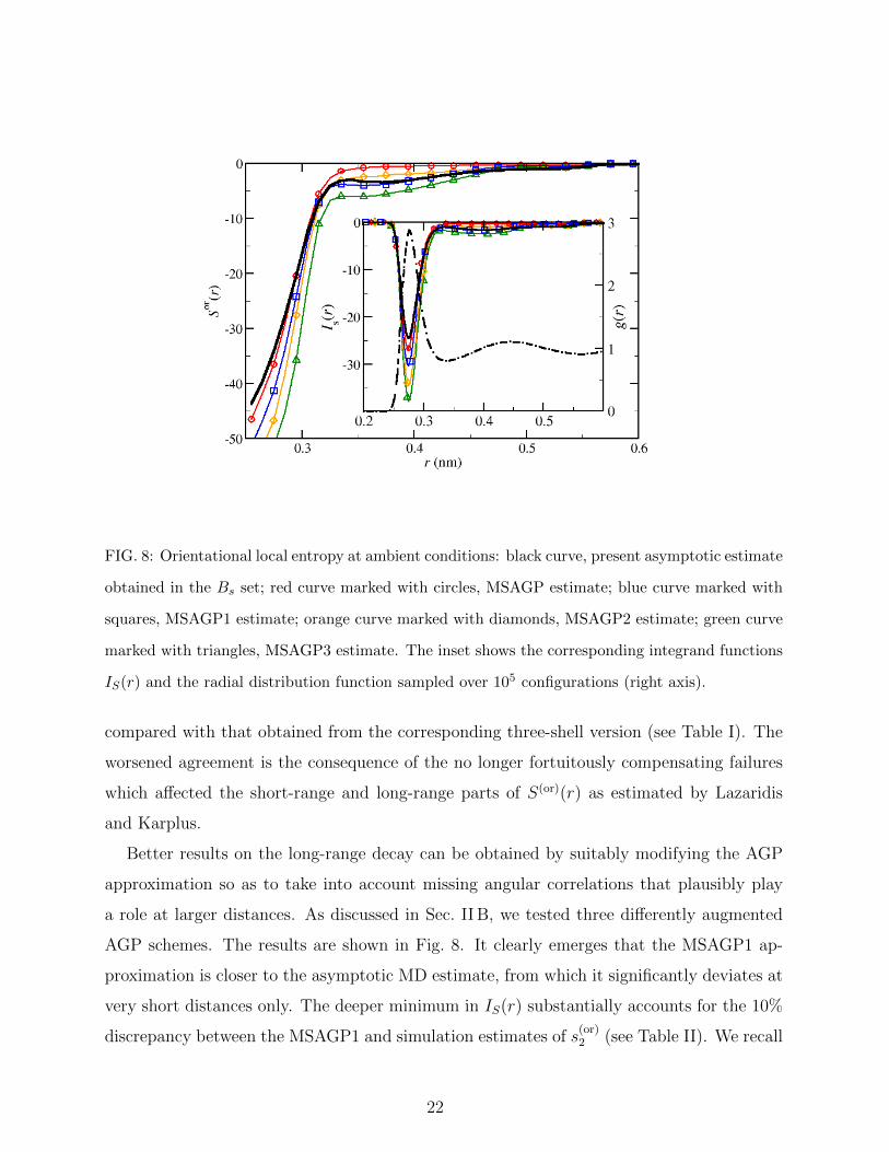
FIG. 8: Orientational local entropy at ambient conditions: black curve, present asymptotic estimate

obtained in the Bs set; red curve marked with circles, MSAGP estimate; blue curve marked with

squares, MSAGP1 estimate; orange curve marked with diamonds, MSAGP2 estimate; green curve

marked with triangles, MSAGP3 estimate. The inset shows the corresponding integrand functions

IS(r) and the radial distribution function sampled over 105 configurations (right axis).

compared with that obtained from the corresponding three-shell version (see Table I). The

worsened agreement is the consequence of the no longer fortuitously compensating failures

which affected the short-range and long-range parts of S(or)(r) as estimated by Lazaridis

and Karplus.

Better results on the long-range decay can be obtained by suitably modifying the AGP

approximation so as to take into account missing angular correlations that plausibly play

a role at larger distances. As discussed in Sec. II B, we tested three differently augmented

AGP schemes. The results are shown in Fig. 8. It clearly emerges that the MSAGP1 ap-

proximation is closer to the asymptotic MD estimate, from which it significantly deviates at

very short distances only. The deeper minimum in IS(r) substantially accounts for the 10%

discrepancy between the MSAGP1 and simulation estimates of s(or)2 (see Table II). We recall

22

that this particular scheme includes the intramolecular correlation between the angles θ and

χ through the marginal distributions g(θ1, χ1) and g(θ2, χ2) whose role and importance have

been recently highlighted by Wang and coworkers.18 However, their approximation as well as

the F7 factorization scheme also include cross intermolecular correlations between the same

angular pairs, a combination that we also exploited in the MSAGP3 approximation. As seen

from Fig. 8, the inclusion of the marginal distributions g(θ1, χ2) and g(θ2, χ1) worsens the

agreement with the simulation data in that these additional correlations do actually overem-

phasize the structure of S(or)(r) both at small and large distances, producing an even more

profound minimum in IS(r) as well as a more prominent long-range tail. Correspondingly,

the estimated orientational pair entropy drops by more than four entropy units. The major

responsibility of intermolecular (θ, χ) correlations in hollowing out a deeper minimum in the

integrand function is also confirmed by the outcome of the MSAGP2 approximation where

intramolecular (θ, χ) correlations have been neglected.

A significative property shared by all the multi-shell AGP approximations discussed above

is their fast convergence rate as a function of the number of configurations. As seen from

Table III, the estimates of s(or)2 obtained after averaging the marginals over 5× 103 configu-

rations do in fact coincide with those produced with 104 configurations to the first decimal

place.

B. TIP4P water close to the temperature of maximum density

Upon lowering the temperature while keeping the pressure fixed at 1 bar, TIP4P wa-

ter first exhibits the well-known maximum density anomaly at TTMD = 253 ± 5 K before

congealing into ice Ih at Tf = 232 ± 5 K, i.e., about 40 K below the experimental freezing

point.25 At 260 K the average values of the specific density and excess internal energy were

found to be 1.001 g cm−3 and −10.67 kcal mol−1, respectively. At lower temperatures both

the positional and angular order are more enhanced and longer-ranged. The RDF of the

liquid is definitely more structured than at ambient conditions (see Fig. 1) and we consis-

tently found a value for the translational pair entropy (−3.59 e.u.) that is about 18% lower

than that obtained at 300 K. As for the calculation of the orientational pair entropy, we

verified that the fit of σ(r;Nconf) was of comparable accuracy as that achieved at higher

temperature. Also in this case the tail of σ(r;Nconf) turned out to scale as N−1conf at large

23

FIG. 9: Orientational local entropy at P = 1 bar and T = 260 K: black curve, present asymptotic

estimate obtained in the Bs set; red curve marked with circles, MSAGP estimate; blue curve marked

with squares, MSAGP1 estimate; orange curve marked with diamonds, MSAGP2 estimate; green

curve marked with triangles, MSAGP3 estimate. The inset shows the corresponding integrand

functions IS(r) and the radial distribution function sampled over 105 configurations (right axis).

distances. Figure 9 shows the extrapolated OLE and the corresponding integrand function.

The comparison with the approximate estimates obtained from the four AGP schemes that

we have already illustrated in the preceding sections confirms that even at this lower tem-

perature the MSAGP1 approximation more faithfully reproduces the profile of S(or)(r), both

at short and large distances. Correspondingly, the MSAGP1 estimate of the orientational

pair entropy was again found to be closer than the other three approximate estimates to

the asymptotic simulation value, the relative discrepancy being about 7% (see Table II).

We observe that s(or)2 – and, correspondingly, the amount of angular order in water – is

more significantly affected than s(tr)2 by the 40 K temperature drop. In fact, the value of the

orientational pair entropy at 260 K was found to be about 29% lower than that at 300 K.

24

C. TIP4P water at higher pressure

We finally investigated the properties of ambient temperature TIP4P water compressed at

a higher pressure (P = 4 kbar), falling in the range where crystalline Ice II and Ice III phases

become stable at lower temperatures.11,12 We found 1.134 g cm−3 and −10.18 kcal mol−1 for

the average values of the specific density and excess internal energy, respectively. At vari-

ance with the behavior ordinarily observed in simple atomic fluids, the compression largely

disrupts the local order observed in water at lower pressures. The effect on positional corre-

lations is manifest in Fig. 1. Notwithstanding this “antagonist” role played by the pressure,

we found that, upon increasing P from 1 bar to 4 kbar at 300 K, the translational pair en-

tropy dropped from −3.05 e.u. to −3.35 e.u.; the disruption of a relatively ordered network,

which would imply a higher entropy, is more than compensated in this case by the reduc-

tion of available positional states produced by the 15% increase of the specific density. The

decorrelating effect produced by compression is even stronger on angular order, as witnessed

by the moderate increase that was registered instead in the orientational pair entropy (see

Table II), notwithstanding the increase of the density.14

The fit of σ(r;Nconf) turned out to be as accurate as that accomplished in the other

two thermodynamic states. The scaling of the function as N−1conf at large distances was

also confirmed. Figure 10 shows the extrapolated OLE and the corresponding integrand

function. The comparison between the results obtained from the four AGP schemes confirms

once more that even at higher pressures the MSAGP1 approximation is the most reliable

approximation at short as well as large distances, and also provides the most accurate

estimate of the orientational pair entropy.

D. Comparison with experimental data

Table IV presents a comparison between the cumulative pair entropies obtained from the

current MD simulations without resorting to any approximation and the excess entropies of

both TIP4P and ordinary water. The TIP4P values26 of sex were obtained using thermody-

namic integration methods for the calculation of the free energy, as extensively discussed in

Ref. 12, while the experimental values follow from the data for the absolute entropy tabulated

in Ref. 27, after subtracting the ideal-gas entropy. This latter contribution was calculated

25

FIG. 10: Orientational local entropy at P = 4 kbar and T = 300 K: black curve, present asymptotic

estimate obtained in the Bs set; red curve marked with circles, MSAGP estimate; blue curve marked

with squares, MSAGP1 estimate; orange curve marked with diamonds, MSAGP2 estimate; green

curve marked with triangles, MSAGP3 estimate. The inset shows the corresponding integrand

functions IS(r) and the radial distribution function sampled over 105 configurations (right axis).

from Eq. (6.5) of Ref. 27, which parametrizes the ideal Helmholtz free energy. Note that

the experimental estimate of the excess entropy at 260 K obviously refers to metastable

undercooled water and was obtained upon extrapolating the values of the specific density

and of the absolute entropy below the freezing temperature. We first observe that the pair

entropy decreases upon lowering the temperature. The effect produced by an increase of

the pressure on the local order of the liquid is more subtle, as already discussed above and

more systematically analyzed in Ref. 14. In this specific instance the effect is almost null,

since the difference of 0.1 e.u. is presumably within the numerical uncertainty of the calcu-

lation. It should further be noted that the almost equal values found for s2 at 300 K across

the 4 kbar pressure gap is the outcome of differing relative weights of the translational and

orientational pair entropies.

26

TABLE IV: Pair and excess entropies

T (K) P (bar) Entropies (e.u.)

s2 [TIP4P] sex[TIP4P]a sex [Expt.]b

260 1× 100 −18.39 −17.00 −15.73c

300 1× 100 −14.57 −14.61 −13.99

300 4× 103 −14.68 −15.14 −14.38

aData from Ref. 26, reported with an estimated uncertainty of 0.06 e.u..bEstimates obtained from the data available in Ref. 27.cEstimate obtained upon extrapolating the properties of liquid water below the freezing point.

As shown in Table IV, at 260 K the pair entropy actually overcomes the excess entropy:

this implies a positive value of the so-called “residual multiparticle entropy” (RMPE), a

quantity defined as the difference between sex and s2.19 As diffusely documented in the lit-

erature, a positive RMPE is evidence of a highly structured liquid.13,28 On the other hand,

at 300 K the RMPE of TIP4P water almost vanishes at ambient pressure conditions, while

being negative at 4 kbar but less than 3% of the total excess entropy. We remark that, as

previously noted by Lazaridis and Karplus,9 a small value of the RMPE does not neces-

sarily imply that triplet or higher-order correlations do not play a role in determining the

microscopic structure of the liquid. In fact, their overall contribution to the configurational

entropy of a given substance may well be small or may even sum up to zero in some thermo-

dynamic points or regions of the phase diagram, despite the fact that distribution functions

beyond the pair one do not trivially reduce to the mere product of lower-order distribution

functions.

It appears from Table IV that at 300 K the pair entropy of TIP4P water provides fairly

good estimates of the excess entropy of ordinary water. However, we are also aware that the

agreement between the model and experimental data might be partially biased by the 40 K

“shift” towards lower temperatures of the phase diagram predicted by the TIP4P model of

water relatively to that of ordinary water.

27

V. CONCLUDING REMARKS

In this paper we have presented a Molecular Dynamics calculation of the pair entropy

of liquid water, modeled with the four-point transferable intermolecular potential (TIP4P)

at three distinct thermodynamic states, corresponding to different values of temperature

and pressure. The pair entropy is an integrated measure of two-body density correlations

and represents the predominant contribution to the configurational entropy of a liquid. As

such, it can be confidently used as a local structural estimate of the total configurational

entropy: local, in that it does not call for an integration of the properties of the liquid along

a thermodynamic path; structural, since it provides a direct connection between entropy and

spatial order as monitored by the pair distribution function. This is the first aspect that

we have put under scrutiny in this paper by extending preexisting analyses carried out for

TIP4P water to thermodynamic states other than ambient conditions. Our new results for

the orientational pair entropy follow from the calculation of the five-dimensional histogram

that we obtained upon sampling, at given temperature and pressure, the configurations

corresponding to different relative orientations of a generic water molecule with respect to

a reference one, while keeping their centers of mass at a fixed distance. An intrinsic bias

on the present results comes from the histogram bin width, with particular regard to the

angular resolution. Our choice (10), while being that commonly made in previous works

on this subject, arises from a compromise between resolution and statistical quality of the

calculations, a compromise that is unavoidably forced by the need of maintaining the overall

size of the computation at a feasibility level.

A secondary goal of this paper was that of discussing and testing some approximate

schemes for the orientational distribution function that are based on the calculation of

lower-order marginals, given the heavy computational task one has to face with in a full-size

calculation. In this respect, we have analyzed the performance of a number of factoriza-

tions that partially modify the “adjusted gas phase approximation” originally proposed by

Lazaridis and Karplus.9 We found that the best results, as far as both the orientational local

entropy and its integrated value are concerned, were obtained at all of the three sampled

thermodynamic states when using the so-called MSAGP1 approximation, which includes in-

tramolecular correlations between the angle formed by the dipole vector of a water molecule

and the intermolecular axis, and the angle describing the rotation of the same molecule

28

about its own dipole vector. We emphasize that the MSAGP1 estimates were obtained

upon sampling the marginal distribution functions over 104 configurations only and appear

to underestimate the corresponding “exact” Molecular Dynamics values – which were ob-

tained with a sampling carried out over a ten times larger number of configurations – by

12% at the most.

On the other hand, we have also verified that including the intermolecular contribution

which arises from cross correlations between the same angles mentioned above but measured

on different molecules does actually worsen the agreement with the Molecular Dynamics

results in that the ensuing modified scheme (MSAGP3) manifestly overestimates the degree

of orientational order present in the liquid in a systematic way.

VI. ACKNOWLEDGMENTS

E. G. acknowledges a Ph.D. grant from CNISM (Italy) and the scientific hospitality of the

Universite Pierre et Marie Curie (Paris, France) in 2008 during a six-month visit cofunded

by the Erasmus/Socrates program, and also thanks Drs. Rubens Esposito and Dino Costa

for numerical assistance at different stages of this work. P. V. G. thanks Prof. Carlos Vega

for providing some reference thermodynamic data on the TIP4P model and Dr. Lingle Wang

for some clarifying comments on the calculation of the orientational entropies with the kth

nearest-neighbor method. The authors gratefully acknowledge the allocation of computer

time from the French National Supercomputing Facility IDRIS, within the projects CP9-

81387 and CP9-91387, and from the “Centro di Calcolo Elettronico ‘Attilio Villari’ della

Universita degli Studi di Messina”.

∗ Electronic address: emanuela.giuffre@unime.it

† Electronic address: santi.prestipino@unime.it

‡ Electronic address: saija@me.cnr.it

§ Electronic address: marco.saitta@impmc.upmc.fr

¶ Electronic address: paolo.giaquinta@unime.it

1 Ben-Naim, A. Molecular Theory of Water and Aqueous Solutions – Part 1: Understanding

Water ; World Scientific: Singapore, 2009.

29

2 Ball, P. Nature 2008, 452, 291.

3 Green, H. S. The Molecular Theory of Fluids; North-Holland: Amsterdam, The Netherlands,

1952.

4 Stratonovich, R. L. Sov. Phys. JETP 1955, 28, 409.

5 Nettleton, R. E.; Green, M. S. J. Chem. Phys. 1958, 29, 1365.

6 Yvon, J. Correlations and Entropy in Classical Statistical Mechanics; Pergamon Press: Oxford,

United Kingdom, 1969.

7 Baranyai, A.; Evans, D. J. Phys. Rev. A 1989, 40, 3817.

8 Prestipino, S.; Giaquinta, P. V. J. Stat. Phys. 1999, 96, 135; 2000, 98, 507.

9 Lazaridis, T.; Karplus, M. J. Chem. Phys. 1996, 105, 4294.

10 Jorgensen, W. L.; Chandrasekhar, J; Madura, J. D.; Impey, R. W.; Klein, M. L. J. Chem. Phys.

1983, 79, 926.

11 Sanz, E.; Vega, C.; Abascal, J. L. F.; MacDowell, L. G. J. Chem. Phys. 2004, 121, 1165.

12 Vega, C.; Sanz, E.; Abascal, J. L. F.; Noya, E. G. J. Phys.: Condens. Matter 2008, 2, 153101.

13 Saija, F.; Saitta, A. M.; Giaquinta, P. V. J. Chem. Phys. 2003, 119, 3587.

14 Esposito, R.; Saija, F.; Saitta, A. M.; Giaquinta, P. V. Phys. Rev. E 2006, 73, 040502(R).

15 Zielkiewicz, J. J. Chem. Phys. 2005, 123, 104501.

16 Zielkiewicz, J. J. Chem. Phys. 2006, 124, 109901.

17 Zielkiewicz, J. J. Phys. Chem. B 2008, 112, 7810.

18 Wang, L.; Abel, R.; Friesner, R. A.; Berne, B. J. J. Chem. Theory Comput. 2009, 5, 1462.

19 Giaquinta, P. V.; Giunta, G. Physica A 1992, 187, 145.

20 Giaquinta, P. V.; Giunta, G.; Prestipino Giarritta, S. Phys. Rev. A 1992, 45, R6966.

21 Jakse, N.; Charpentier, I. Phys. Rev. E 2003, 67, 061203.

22 Prestipino, S.; Giaquinta, P. V. J. Stat. Mech. 2004, P09008.

23 Martyna, G. J.; Tuckerman, M. E.; Klein, M. L. PINY MD (c) Simulation Package c© 2002.

24 IUPAC Compendium of Chemical Terminology, 2nd ed. (the ”Gold Book”). XML on-line cor-

rected version: http://goldbook.iupac.org/E02151.html (accessed Nov 23, 2009).

25 Vega, C.; Abascal, J. L. F. J. Chem. Phys. 2005, 123, 144504.

26 Vega, C. 2009, private communication.

27 Wagner, W.; Pruss, A. J. Phys. Chem. Ref. Data 2002, 31, 387.

28 Giaquinta, P. V. Entropy revisited: The interplay between entropy and correlations. In High-

30

lights in the Quantum Theory of Condensed Matter ; Beltram, F., Ed.; Publications of the Scuola

Normale Superiore (Selections); Edizioni della Normale: Pisa, Italy, 2005; Vol. 1, pp. 9-14; see

also the introduction and the bibliography in: Giaquinta, P. V. Entropy 2008, 10, 248.

31