University of Nebraska - LincolnDigitalCommons@University of Nebraska - Lincoln

Faculty Publications: Agricultural Economics Agricultural Economics Department

9-29-2010

Environmental Efficiency Among Corn EthanolPlantsJuan P. SesmeroPurdue University - Main Campus, jsesmero@purdue.edu

Richard K. PerrinUniversity of Nebraska, rperrin@unl.edu

Lilyan E. FulginitiUniversity of Nebraska, lfulginiti@unl.edu

This Article is brought to you for free and open access by the Agricultural Economics Department at DigitalCommons@University of Nebraska -Lincoln. It has been accepted for inclusion in Faculty Publications: Agricultural Economics by an authorized administrator ofDigitalCommons@University of Nebraska - Lincoln.

Sesmero, Juan P.; Perrin, Richard K.; and Fulginiti, Lilyan E., "Environmental Efficiency Among Corn Ethanol Plants" (2010). FacultyPublications: Agricultural Economics. Paper 105.http://digitalcommons.unl.edu/ageconfacpub/105

1

Environmental Efficiency Among Corn Ethanol Plants

Juan P Sesmero*,1, Richard K Perrin2 and Lilyan E Fulginiti3

1 Department of Agricultural Economics, Purdue University, IN 47907-2056, USA

2, 3 Department of Agricultural Economics, University of Nebraska, Lincoln, NE 68583, USA

* Corresponding author. KRAN 591A, West Lafayette, IN 47907-2056, USA. E-mail address: jsesmero@purdue.edu . Tel.: 1(765) 494-7545.

2

Abstract

Economic viability of the US corn ethanol industry depends on prices, technical and

economic efficiency of plants and on continuation of policy support. Public policy

support is tied to the environmental efficiency of plants measured as their impact on

emissions of greenhouse gases. This study evaluates the environmental efficiency of

seven recently constructed ethanol plants in the North Central region of the U.S., using

nonparametric data envelopment analysis (DEA). The minimum level of GHG emissions

(per gallon of ethanol produced) feasible with the available technology is calculated for

each plant and this level is used to decompose environmental efficiency into its technical

and allocative sources. Results show that, on average, plants in our sample may be able to

reduce GHG emissions by a maximum of 6% or by 3,116 tons per quarter. Input and

output allocations that maximize returns over operating costs (ROOC) are also found

based on observed prices. The environmentally efficient allocation, the ROOC

maximizing allocation, and the observed allocation for each plant are combined to

calculate economic (shadow) cost of reducing greenhouse gas emissions. These shadow

costs gauge the extent to which there is a trade off or a complementarity between

environmental and economic targets. Results reveal that, at current activity levels, plants

may have room for simultaneous improvement of environmental efficiency and economic

profitability.

Keywords: ethanol carbon footprint; environmental efficiency; shadow cost; data

envelopment analysis.

3

1. Introduction

The U.S. corn ethanol industry has benefited from government support due to its

potential to achieve a rather wide set of goals: mitigating emissions of greenhouse gases

(GHG), achieving energy security (diversifying energy sources), improving farm incomes

and fostering rural development among others. Continuation of policy support, however,

is being debated due to doubts about the direct and indirect GHG effects of the industry.

Moreover, the capacity of the industry to reduce GHG emissions per gallon of ethanol

produced may also determine the opportunities opened to it in future carbon markets and

in the National Renewable Fuel Standard program. This study provides information

relevant to these issues by measuring the environmental performance of the industry in

terms of GHG emissions per gallon produced and the economic cost (shadow price) of

GHG reductions.

Input requirements and byproducts’ yield per gallon of ethanol produced are critical

in determining environmental performance. Previous studies have addressed the issue of

input requirements and byproducts’ yield of ethanol plants. Using engineering data

McAloon et al. (2000) and Kwiatkowski et al. (2006) measured considerable

improvement in plant efficiency between 2000 and 2006. Shapouri, et al. (2005) reported

input requirements and cost data based on a USDA sponsored survey of plants for the

year 2002. Wang et al. (2007) and Plevin et al. (2008), reported results based on

spreadsheet models of the industry (GREET and BEACCON, respectively). Pimentel et

al. (2005) and Eidman (2007) reported average performances of plants although they do

not clearly indicate the sources of their estimates. Finally Perrin et al. (2009) reported

results on input requirements, operating costs, and operating revenues based on a survey

4

of seven dry grind plants in the Midwest during 2006 and 2007. This study does not

report however results on the carbon footprint of ethanol plants.

With the exception of Shapouri et al. (2005) and Perrin et al. (2009) all of these

studies reported values corresponding to the average plant (not individual plants) which

prevents comparison of relative performances. In addition, it is generally believed that the

industry has become more efficient and technologically homogeneous since 2005. Since

the data used in Shapouri et al. (2005) was collected in 2002 it may not be representative

of current technologies in the industry. In contrast to Shapouri et al. (2005), Perrin et al.

(2009) surveyed plants in operation during 2006 and 2007 and employed a much more

restrictive sampling criterion (discussed below) which yielded a modern and

technologically homogenous sample of plants. This sample is believed to be more

representative of current technologies and is, hence, our data of choice to assess the

environmental performance of plants. Based on these data the present study evaluates the

environmental efficiency of seven recently constructed ethanol plants in the North

Central region of the U.S. The returns over operating costs (ROOC)1

that may be gained

or lost by plants as a consequence of the effort to reach a given environmental target are

also calculated and discussed.

2. Materials and Method

2.1. Data

The environmental performance of a plant is evaluated on the basis of emission of

greenhouse gases associated with its productive activity. Greenhouse gas emissions from

1 We evaluate economic performance based on returns over operating costs rather than profits. This is because capital costs are not included in our analysis.

5

plants were not directly measured but rather calculated based on observable inputs and

outputs corresponding to each plant. In addition concerns regarding the environmental

impact of ethanol production refer to life cycle2 GHG emissions and not only those

emissions at the processing stage. Therefore we evaluate life cycle GHG emissions

associated with observable inputs and outputs. Our observations consist of 33 quarterly

reports of input and output quantities and prices from a sample of seven Midwest ethanol

plants. Following the non parametric efficiency literature we refer to each observation as

a decision making unit (DMU). Plants produce 3 outputs (ethanol, dry distillers grains

with solubles (DDGS), and modified wet distillers grains with solubles (MWDGS)) using

7 inputs3

(corn, natural gas, electricity, labor, denaturant, chemicals, and “other

processing costs”).

2.2. Ethanol Plants: Characteristics

Table 1 presents some quarterly characteristics of the seven dry grind ethanol plants

surveyed. According to Table 1 the plants produced an average rate equivalent to 53.1

million gallons of ethanol per year, with a range from 42.5 million gallons per year to

88.1 million gallons per year. The period surveyed included from the third quarter of

2006 until the fourth quarter of 2007 (six consecutive quarters). In addition plants could

be differentiated by how much byproduct they sold as DDGS (10% moisture) compared

2 “Life cycle” in this case includes emissions taking place at three stages of the production process: corn production (farmers), ethanol production (biorefinery), and feedlot (byproducts from ethanol plants are given a credit for replacing corn as feed in livestock production). 3 Results of our survey contained total expenditures in labor, denaturant, chemicals, and other processing costs. As a result we calculated implicit quantities for these inputs dividing total expenditures by their corresponding price indexes. Labor and management price index associated to the Basic Chemical Manufacturing Industries was obtained from http://www.bls.gov/oes/current/naics4_325100.htm#b00-0002. Denaturant, chemicals and other processing costs were calculated based on the Producer Input Price Index for “All other basic inorganic chemicals”, http://www.bls.gov/pPI/.

6

to MWDGS (55% moisture). Variation on this variable was significant, averaging 54% of

byproduct sold as DDGS, but ranging from one plant that sold absolutely no byproduct as

DDGS to another plant that sold nearly all byproduct (97%) as DDGS.

Finally, Table 1 briefly characterizes plant marketing strategies. In purchasing input

feedstock, five of the six plants purchased corn via customer contracts. Similarly, in

selling ethanol, five of the six plants used third parties or agents. Byproduct marketing

across plants displayed a higher degree of variance. Marketing of DDGS was split fairly

evenly between spot markets and third parties/agents. An even higher variability was

observed for MWDGS, where no one marketing strategy (spot market, customer contract,

or third party/agent) was significantly more prevalent across plants than any other.

Table 2 displays descriptive statistics of inputs used and outputs produced by the 33

DMUs in our sample. As mentioned before the basic observations in this study

corresponds to a plant in a given quarter; so two quarters of the same plant are considered

as two different observations as are two plants in the same quarter.

2.3. Environmental Performance of Ethanol Plants

2.3.1. Emissions Measurement

No direct measurements of GHG emissions are available in this industry; however

they can be calculated using engineering relationships. A number of computer packages

have been developed to facilitate these calculations (Wang et al. 2007; Farrell et al.

2006). We used the Biofuels Energy Systems Simulator4

4 BESS is a software developed by a team of specialists in the Agronomy Department at the University of Nebraska, Lincoln (Liska, et al, 2009a, 2009b,

(BESS). The BESS model

includes all GHG emissions from the burning of fossil fuels used directly in crop

http://www.bess.unl.edu/ )

7

production, grain transportation, biorefinery energy use, and coproduct transport. All

upstream energy costs and associated GHG emissions with production of fossil fuels,

fertilizer inputs, and electricity used in the production life cycle are also included. Since

these calculations involve modeling of crop production and feedlot and these display

regional differences, BESS includes regional scenarios and an average scenario for the

whole Midwest region. Plants in our sample are scattered across the Midwest and, hence,

we have used scenario 2 in BESS “US Midwest average UNL” which is deemed

representative of the whole region.

The BESS calculations of GHG emissions associated with a dry mill plant are

equivalent to the following linear relationship:

0.00668274 0.063015823 0.0007445 0.000316916

0.4197522186 0.407868 Mg c NG elect Eth

DDGS MWDGS

GHG x x x uu u

= + + +

− − (1)

Where MgGHG represents megagrams of life cycle CO2 equivalent greenhouse gases, cx

is bushels of corn used by the plant, DDGSu and MWDGSu are tons of byproduct sold as

dried and modified wet respectively by the plant, NGx is the total amount of natural gas

used by the plant measured in MMBTUs, electx is total amount of kilowatt hours (kwh) of

electricity used by the plant, and Ethu is the plant’s ethanol production in gallons.

Eq. (1) states that a bushel of corn used in a biorefinery is associated with about

0.0067 megagrams of GHG emitted during the production of that bushel. DDGS and

MWDGS have a positive and a negative component. The former is due to additional

energy used in reducing moisture.5

5 In particular MWDGS require the use of electricity to centrifuge the wet byproduct and DDGS require the use of natural gas for heating and drying the wet byproduct after the centrifuge.

The latter are “credits” attributed to byproducts (i.e.

8

reductions in GHG) due to the replacement of corn that would have been fed to livestock

had the byproduct not been sold. The coefficient for ethanol production represents the

combination of emissions associated with depreciable capital ( 0.0002050 ) and freight for

grain transportation ( 0.000111916 ), expressed on a per gallon basis.

Eq. (1) includes outputs ( ), ,j j j jEth MWDGS DDGSu u u u= and a pollution increasing subset of

all inputs used by ethanol plants6 ( ), ,j j j jp c NG electx x x x= denoted by , where subindex p

indicates pollutant. We can now re express Eq. (1) in vector notation. To do so we

partition inputs and outputs into a column vector of pollution increasing inputs and output

( ), , ,j j j j jc NG elect Etha x x x u= ' and a column vector of pollution reducing byproducts

( ),j j jb MWDGS DDGSu u u= '. The level of greenhouse gas emissions associated with a particular

plant j as a function of observable inputs and outputs can be expressed as:

j j jbGHG a uα β= + (2)

Where ( )0.0066,0.0630,0.00074,0.000316α = is the 1x4 row vector of coefficients

associated with pollution increasing categories ja , and ( )0.419752, 0.407868β = − − is

the 1x2 row vector of coefficients associated with pollution reducing byproducts jbu .

2.3.2. Characterization of Potential Ethanol Technology From Individual Plant Data

Plants are constrained by a technology transforming a vector of N inputs

( ) NNxxxx +ℜ∈= ,...,, 21 into a vector of M outputs ( ) M

Muuuu +ℜ∈= ,...,, 21 . Observed

combinations of inputs used and outputs produced ( ),j jx u are taken to be representative 6 As described before ethanol plants use 7 inputs in production. However only three of them increase life-cycle emissions of GHGs: corn, natural gas, and electricity.

9

points from the feasible ethanol technology. In this study we use data envelopment

analysis (DEA) to infer the boundaries of the feasible technology set from the observed

points, following the notation in Färe, et al.

Observations from the technology consist of a sample of 33 DMUs producing 3

outputs and using 7 inputs. The production technology can be represented by a graph

denoting the collection of all feasible input and output vectors:

( ) ( ){ }7 3, :GR x u x L u++= ∈ℜ ∈

Where ( )uL , is the input correspondence which is defined as the collection of all input

vectors Nx +ℜ∈ that yield at least output vector Mu +ℜ∈ .

The frontier of the graph GR and observed levels of inputs and outputs will serve as

references for environmental efficiency assessment.

2.3.3. Environmental Efficiency Measurement

A given DMU (call it j) is deemed more environmentally efficient whenever it

chooses a feasible (subject to the graph) combination of inputs and byproducts (DDGS

and MWDGS) that results in lower GHG emissions while maintaining its ethanol

production level at the observed value denoted by jEthu . Fixing ethanol production to its

observed level, and assuming variable returns to scale and strong disposability of inputs

and outputs the graph can be denoted by:

( ) ( )33

1, , , : , , , 1, 1,...,33j j j j j j

Eth b b Eth Ethj

GR V S u x u u zM x zN zu u z j=

= ≤ ≥ = = =

∑ (3)

10

Where z depicts a row vector of 33 intensity variables, bM is the 33x2 matrix of

observed byproducts, jbu is the 1x2 vector of observed byproducts corresponding to the

jth DMU, N is the 33x7 matrix of observed inputs, , jx is the 1x7 vector of observed

inputs corresponding to the jth DMU, Ethu is the 33x1 vector of observed outputs, and

jEthu is the observed ethanol production by observation j.

We define the set of all combinations of corn, gas, electricity and byproducts that

result in lower emissions than those actually produced by the thj DMU as:

( ) ( ){ }, , , :j j j j j j j j j jg p b Eth p b x p b x p bGHG x u u x u x u x uα β α β′ ′ ′= + ≤ + (4)

Where xα is a subset of the vector α previously defined which does not include the

coefficient for ethanol, i.e. ( )0.006682,0.063015,0.000744xα = and the rest is as

before.7

From Eq. (4) we can derive an isopollution line in DDGS and corn space, i.e.

combinations of DDGS and corn that result in the same level of emissions keeping

everything else constant. Fig. 1 depicts this set graphically in the corn and DDGS space

(i.e. keeping everything else in the GHG equation fixed). The set

jgGHG consists of all

those points above the isopollution line as indicated by the arrows with direction

northwest.

7 We denote the coefficient associated with ethanol by γ =0.000316. Ethanol production and its associated

coefficient are included in both sets. However, since ethanol is fixed at the observed level jEthu , the

complete version of the inequality is j j j j j jx p b Eth x p b Ethx u u x u uα β γ α β γ′ ′+ + ≤ + + which after

elimination is equivalent to the expression in (4).

11

In Fig. 1 the feasible technology set is represented by a graph displaying variable

returns to scale and strong disposability of inputs and outputs as indicated by the arrows

moving from the frontier ( ( )DDGS cu f x= ) with direction southeast. As clearly seen in

Fig. 1, the set jgGHG includes combinations outside the graph and hence not attainable

by DMUs in the sample. The subset of observations in jgGHG that belong to the graph

and are hence attainable by DMUs is depicted by the intersection of both sets delimited

by the bold lines in Fig. 1:

( ) ( ), , , ,j j j j jg p b Eth EthGHG x u u GR V S u∩ (5)

The thj DMU could choose any alternative production plan within the area denoted

by the bold lines to produce its ethanol production level, achieving a reduction in

emissions while increasing DDGS or reducing corn or both simultaneously. In this study,

the environmental technically efficient projection of a given observation to the boundary

of the technology set follows a hyperbolic path defined by equiproportional reductions in

inputs and increases in byproducts. The value of the proportionate change necessary to

encounter the boundary, jgETE , is defined as the environmental technical efficiency of

plant j:

( ) ( ) ( ){ }1, , min : , , ,j j j j j j jg p b Eth g p b EthETE x u u GHG x u GR V S uλ λ λ−= ∩ ≠ ∅ (6)

Where λ is a scalar defining the proportionate changes and the rest is as before. We

calculated the value of ( ), ,j j j jg p b EthETE x u u using MATLAB as indicated in Appendix A.

12

Environmental technical efficiency defined in Eq. (6) is illustrated in Fig. 2 by the

distance from ( ),j jc DDGSx u to point A which corresponds to the environmental technically

efficient allocation in corn and DDGS space.

Note however that point A does not correspond to the minimum feasible GHG level

since it does not coincide with the point of tangency between the isopollution and the

graph (point B). The allocation that achieves the minimum level of GHG emissions

subject to the graph is called the overall environmental efficient allocation.

Technically, we define this minimum feasible level of GHG emissions as:

( ) ( ){ },min + . . ( , ) , ,

p b

j j j jEth x p b Eth p b Ethx u

GHG u GHG x u u s t x u GR V S uα β γ= = + ∈ (7)

Where ( )j jEthGHG u denotes minimum emissions attainable by j subject to observed

ethanol production jEthu , px is the vector of pollution increasing inputs, bu is the vector

of byproducts and the rest is as defined before. The empirical calculation of Eq. (7) is

described in Appendix B.

Overall environmental efficiency, jgE , is measured by the hyperbolic distance

between a given observation j and the isopollution line corresponding to ( )j jEthGHG u .

The hyperbolic distance is computed through calculation of the reduction of observed

inputs and equiproportional expansion of observed byproducts such that the isopollution

corresponding to ( )j jEthGHG u is reached. This is illustrated by Fig. 3 where overall

environmental efficiency is the distance between ( ),j jc DDGSx u and point C.

13

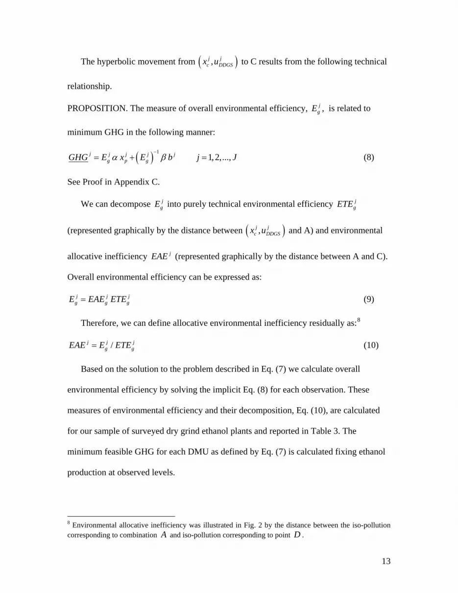
The hyperbolic movement from ( ),j jc DDGSx u to C results from the following technical

relationship.

PROPOSITION. The measure of overall environmental efficiency, jgE , is related to

minimum GHG in the following manner:

( ) 1 1, 2,...,j j j j j

g p gGHG E x E b j Jα β−

= + = (8)

See Proof in Appendix C.

We can decompose jgE into purely technical environmental efficiency j

gETE

(represented graphically by the distance between ( ),j jc DDGSx u and A) and environmental

allocative inefficiency jEAE (represented graphically by the distance between A and C).

Overall environmental efficiency can be expressed as:

j j jg g gE EAE ETE= (9)

Therefore, we can define allocative environmental inefficiency residually as:8

/j j jg gEAE E ETE=

(10)

Based on the solution to the problem described in Eq. (7) we calculate overall

environmental efficiency by solving the implicit Eq. (8) for each observation. These

measures of environmental efficiency and their decomposition, Eq. (10), are calculated

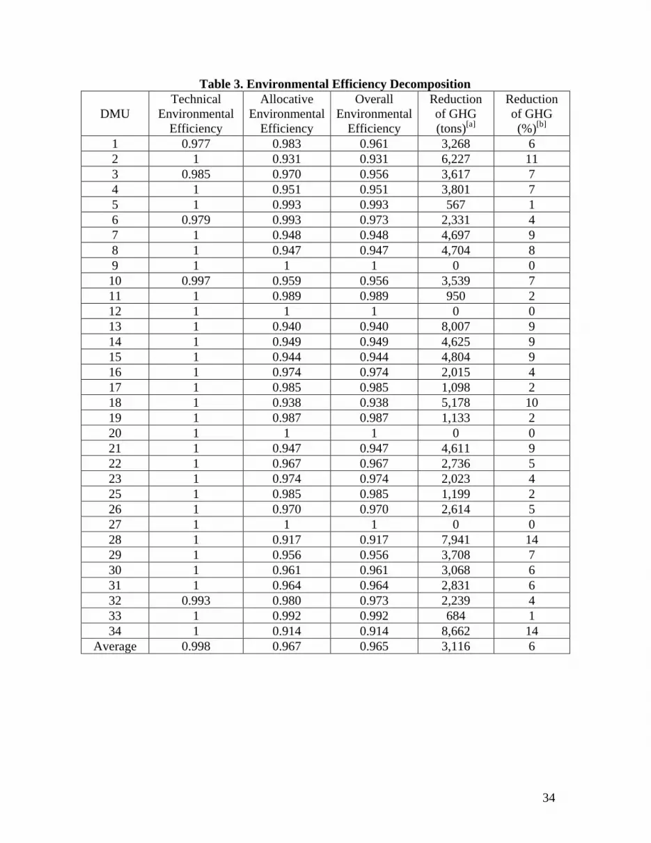
for our sample of surveyed dry grind ethanol plants and reported in Table 3. The

minimum feasible GHG for each DMU as defined by Eq. (7) is calculated fixing ethanol

production at observed levels.

8 Environmental allocative inefficiency was illustrated in Fig. 2 by the distance between the iso-pollution corresponding to combination A and iso-pollution corresponding to point D .

14

2.4. ROOC and Environmental Targets: Trade off or Complementarity?

From Eq. (2) there is a clear relationship between GHG and the combination of inputs

and byproducts. But there is also a relationship between combinations of inputs and

byproducts and the level of ROOC. Therefore, in general, a change in GHG levels

through reallocation of inputs and byproducts would bring about a change in ROOC. For

a given level of ethanol production, the shadow price of GHG mitigation is the change in

ROOC per unit change in GHG levels. The change in ROOC denotes the plant's

maximum willingness to pay (WTP) for a permit to emit GHG. We define the shadow

price of a ton of GHG as:

1 0

1 0 1 0

j jj

GHG j j j jWTPSV

GHG GHG GHG GHGπ π−

= =− −

(11)

Where WTP is willingness to pay for changing emissions from 0jGHG to 1

jGHG . 0jGHG

denotes the original level of GHG and 0jπ the corresponding level of ROOC. 1

jGHG is

the “targeted” level of GHG and 1jπ denotes ROOC at this targeted level. GHG level will

be targeted at the minimum GHG (i.e. 1jGHG = jGHG ), or alternatively at the level

corresponding to maximum achievable ROOC by firm j, *jπ , which we designate as

*jGHG .

2.4.1. Shadow Cost from Observed to ROOC Maximizing Allocation

We define the ROOC maximizing combination of inputs and byproducts (subject to a

given level of ethanol production to make it comparable with the GHG minimizing

combination) as the allocation that solves the following problem:

15

( )( ) { } ( ) ( )* ,, , , , , , , ,

b

j j j j j j j j j jEth Eth Eth Eth b b Ethx u

r p r GR V S u Max r u r u p x s.t. u x GR V S uπ = + − ∈ (12)

Where jEthr is the observed price of ethanol obtained by observation j, j

Ethu is the

observed level of ethanol production by j, bu is the 2x1 column vector of variable outputs

(DDGS and MWDGS), jr represents the 1x2 vector of observed prices of variable

outputs (byproducts)9 x obtained by observation j, is the 1x7 vector of variable inputs

(corn, natural gas, electricity, labor, denaturant, chemicals, and “other processing costs”),

and jp represents the 1x7 vector of observed prices of variable inputs paid by j.

Quantities of labor, denaturant, chemicals and others needed to calculate GR are

obtained implicitly dividing total expenditures in these categories by their price indexes

described in footnote 2. Prices for these categories in equation (12) are also those in

footnote 2. We will denote the allocation that solves Eq. (12) with ethanol fixed at the

observed level by { }* *( , )j jx u . The level *jGHG is calculated by inserting these values

into (2).

We define the shadow value of GHG emissions associated with moving from the

observed allocation to the ROOC maximizing allocation as:

*

*

j jj

GHG j jSVGHG GHG

π π−=

− (13)

An alternative shadow cost to Eq. (13) is that which is incurred by moving from the

observed to the GHG minimizing combination of inputs and byproducts.

9 Three DMUs in our sample did not sell dried byproducts (they sold 100% MWDGS). Since we did not have reported DDGS prices for those three observations to calculate maximum ROOC we used average prices of DDGS obtained by other DMUs in the same quarter.

16

2.4.2. Shadow Cost from Observed to GHG Minimizing Allocation

The GHG minimizing combination is computed by solving Eq. (7) with ethanol

production fixed at observed levels and minimum GHG denoted by jGHG . ROOC

associated with this allocation (calculated by multiplying the GHG minimizing inputs and

outputs times their respective prices) is designated as jπ .

We define the shadow value of GHG related to a change from the observed to the

GHG minimizing point as:

j jj

GHG j jSV

GHG GHGπ π−

=−

(14)

Finally we consider the shadow value of GHG related to a change from the GHG

minimizing to the ROOC maximizing point.

2.4.3. Shadow Cost from GHG Minimizing to ROOC Maximizing Allocation

Such a change is illustrated in Fig. 4 in the corn and DDGS space. In Fig. 4 the GHG

minimizing combination is represented by point B (the isopollution line is denoted by

jGHG ). If relative prices are those corresponding to the slope of *jπ then ROOC

maximization is achieved at point A and this requires a decrease in corn and DDGS with

respect to the GHG minimizing point. ROOC at A are denoted by *jπ and ROOC at B are

*j jπ π< . Emissions at B are denoted by jGHG and emissions at A are *

jjGHG GHG> .

The shadow value associated with a change from the GHG minimizing combination

to the ROOC maximizing one is defined by:

*

*

j jj

GHG jjSV

GHG GHGπ π−

=−

(15)

17

3. Results and Discussion

3.1. Environmental Performance of Ethanol Plants

Fixing ethanol production at observed levels, measures of environmental efficiency

and their decomposition are calculated for our sample of surveyed dry grind ethanol

plants and reported in Table 3. Results reveal that DMUs are very efficient from a

technical point of view and that most environmental inefficiency comes from allocative

sources. Therefore DMUs seem to have room for GHG reductions mainly by changing

input and output combinations subject to the graph. In particular, the average DMU may

be able to reduce emissions by 6% which amounts to 3,116 tons of CO2 equivalent

GHGs per quarter (or 0.46 pounds per gallon of ethanol produced).

The average DMU in our sample, at observed allocations, displays a GHG intensity

of about 46 gCO2e/MJ. At the GHG minimizing allocation, the average DMU in our

sample displays a GHG intensity of 43 gCO2e/MJ which is 6.5% lower than observed

levels. This intensity is, for example, 55% lower than the target standard established by

California by 2019 (86.27 gCO2e/MJ). It is of interest to know what reallocations of

inputs and byproducts may actually achieve this improvement and we will go back to this

point in detail later.

3.2. ROOC and Environmental Targets

Shadow costs associated with moving from observed to ROOC maximizing

allocations are reported in Table 4. Given the rather large variability across observations

both the median and the average are reported as measures of central tendency. Table 4

18

displays some observations that are unusually high and others unusually low. These

disproportionate deviations from the average are due to changes in inputs that affect

ROOC but do not affect emissions, i.e. labor, denaturant, chemicals, and other processing

costs. These inputs are labor, denaturant, chemicals, and other processing costs. We

classify as “outlier” any observation whose value exceeds the average by more than 3

times the standard deviation.

Since there seems to be a great deal of variability in shadow prices of GHG across

DMUs we have plotted a histogram that shows the approximate distribution of these

values in Fig. 5. The histogram does not take into account those observations deemed as

outliers. We have superimposed to the histogram a normal density function that smoothes

out the distribution. An important conclusion we can extract from Table 4 and Fig. 5 is

the fact that almost all DMUs reduce GHG emissions by moving from observed to

maximum ROOC (negative shadow values). This suggests that, under our convexity

assumptions, most DMUs (including the arithmetic average and the mean of the normal

density function) may be able to increase ROOC and reduce GHG simultaneously which

would in turn imply that these DMUs face no trade off between economic and

environmental goals at current combinations of inputs and byproducts.

The fact that DMUs can rearrange inputs and byproducts in such a way that they can

both increase ROOC and reduce emissions prompts the following questions:

What inputs are reduced or increased and which byproduct is reduced or increased

in such a rearrangement?

Why are plants not exploiting these reallocations that achieve greater ROOC?

19

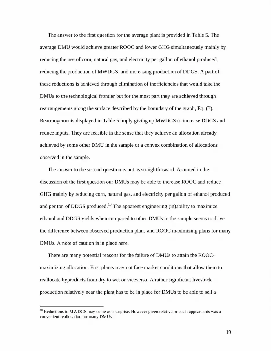
The answer to the first question for the average plant is provided in Table 5. The

average DMU would achieve greater ROOC and lower GHG simultaneously mainly by

reducing the use of corn, natural gas, and electricity per gallon of ethanol produced,

reducing the production of MWDGS, and increasing production of DDGS. A part of

these reductions is achieved through elimination of inefficiencies that would take the

DMUs to the technological frontier but for the most part they are achieved through

rearrangements along the surface described by the boundary of the graph, Eq. (3).

Rearrangements displayed in Table 5 imply giving up MWDGS to increase DDGS and

reduce inputs. They are feasible in the sense that they achieve an allocation already

achieved by some other DMU in the sample or a convex combination of allocations

observed in the sample.

The answer to the second question is not as straightforward. As noted in the

discussion of the first question our DMUs may be able to increase ROOC and reduce

GHG mainly by reducing corn, natural gas, and electricity per gallon of ethanol produced

and per ton of DDGS produced.10

There are many potential reasons for the failure of DMUs to attain the ROOC-

maximizing allocation. First plants may not face market conditions that allow them to

reallocate byproducts from dry to wet or viceversa. A rather significant livestock

production relatively near the plant has to be in place for DMUs to be able to sell a

The apparent engineering (in)ability to maximize

ethanol and DDGS yields when compared to other DMUs in the sample seems to drive

the difference between observed production plans and ROOC maximizing plans for many

DMUs. A note of caution is in place here.

10 Reductions in MWDGS may come as a surprise. However given relative prices it appears this was a convenient reallocation for many DMUs.

20

significant portion of their byproduct as wet. These market constraints are not captured

by our analysis. Second the graph is assumed to be convex in our calculations. Under the

assumption of convexity any difference in performance is attributed to efficiency

differences rather than to technological constraints. However there may be indivisibilities

in the construction and later modifications (expansions or contractions) of plants that

result in non-convexities of the graph, i.e. scaling up or down of production in any

proportion may not be feasible or may be very expensive once capital costs are accounted

for. These non-convexities would prevent plants from choosing the ROOC-maximizing

allocation depicted by the convex graph, rendering economic inefficiencies.

Shadow costs associated with moving from observed to GHG minimizing allocations,

Eq. (14), for each DMU, average, and median are reported in Table 6. Nine DMUs lose

ROOC while reducing GHGs, thus facing positive shadow values of GHGs, meaning a

cost. Seventeen DMUs increase ROOC while reallocating to the minimum GHG level.

The fact that the average willingness to pay for a change in allocation ( j jEπ π− ) is

positive while average change in GHG is negative, results in negative average shadow

values. Table 6 indicates that the average DMU may be able to increase ROOC while

reducing GHG which again seems to suggest unexploited opportunities to improve both

fronts. In particular the average DMU may be able to increase ROOC by about $39 per

ton of GHG reduced. The seventeen firms with negative shadow prices would

presumably be willing to sell permits at any small price, since there is no ROOC lost

from reducing their own GHGs.

Since there seems to be a great deal of variability in shadow prices of GHG across

DMUs we have plotted a histogram that shows the approximate distribution of these

21

values in Fig. 5. The histogram does not take into account those observations deemed as

outliers. The presence of outliers is mainly due, as discussed above, to changes in inputs

affecting ROOC but not GHG, i.e. labor, denaturant, chemicals, and other processing

costs. We have superimposed to the histogram a normal density function that smoothes

out the distribution. Despite the variability across DMUs, the highest frequency of

shadow values (i.e. most of the “mass” of the distribution) appears to be located around

zero. This means that plants are approximately efficient in the sense that they are

operating at levels for which the marginal value of GHG is around zero which is, in turn,

the current GHG price that DMUs face.

According to Table 7 the average DMU achieves minimization of GHG through

substantial reductions in DDGS and MWDGS which in turn allows it to significantly

reduce natural gas and electricity. Finally reductions in corn per gallon of ethanol are also

involved in this GHG minimization. Such reallocations not only achieve reductions in

GHG but also increase ROOC (negative shadow value)

Shadow costs associated with moving from GHG minimizing to ROOC maximizing

allocations, Eq. (15), for each DMU, average and median are reported in Table 8. All

DMUs increase both ROOC and GHGs in moving from low GHG solution to high

ROOC solution. The average DMU would forfeit $1,726 in ROOC for each ton of GHG

reduced, a very high cost of regulation if that firm were required to reduce GHGs. If

DMUs are forced to reduce GHG emissions below ROOC maximizing levels, these

shadow values indicate that they would be willing to purchase permits if the market value

is in the vicinity of $20 to $30 per ton, rather than reduce one ton of GHG emissions. The

histogram (with superimposed normal density) corresponding to Table 8 is plotted in Fig.

22

6. This histogram as the one in Fig. 5 does not take into account those observations

classified as outliers. Again, despite the variability across DMUs, the highest frequency

of shadow values (i.e. most of the “mass” of the distribution) appears to be located

around a very high value.

The reallocation of inputs and byproducts that would take the average DMU from the

GHG minimizing to the ROOC maximizing combination is displayed in Table 9. The

average DMU achieves increases in ROOC mainly through substantial increases in

DDGS which in turn entails increases in natural gas and electricity, and reductions in

MWDGS. Another very important component of ROOC increases is reductions of corn

per gallon of ethanol produced.

Results for the average DMU in Tables 4, 6, and 8 can be combined to recover the

shape of the relationship between GHG and ROOC. Plotting the three averages in the

GHG and ROOC space yields the graph in Fig. 7. We denote the observed combination

of the average by ( ),j jGHG π , the ROOC maximizing combination by ( )* *,j jGHG π , and

the GHG minimizing combination by ( ),j jGHG π . There seems to be room for

simultaneous improvement of environmental and economic performance, as previously

indicated in discussions of Tables 4 and 6. However, if the average firm were able to

adjust inputs and byproducts to the ROOC maximizing combination, it would face an

intense trade off described just above.

4. Conclusions

The purpose of this study was to contribute to the ongoing debate regarding the merits

and potential of the ethanol industry in the US by investigating the current environmental

23

performance at the individual plant level, the potential for improvement in this

performance and its effects on the industry’s overall emissions of greenhouse gases.

Several important conclusions can be drawn from this study. First, our results suggest

that decision making units (DMUs) may have some room for improving environmental

performance. However since plants are technically very efficient, most of this

improvement has to come from changes in combinations of inputs and byproducts along

the frontier (reduction in environmental allocative inefficiencies). By eliminating

allocative inefficiencies the average DMU could apparently decrease emissions by 6%,

which amounts to about 3,116 tons of CO2 equivalent GHG.

Negative shadow values of GHG from observed to ROOC maximizing combinations

reveal that at current operating levels DMUs may be able to increase ROOC and reduce

GHG simultaneously by reaching the “best practice” in the sample. Plants may not be

switching to the ROOC maximizing combination because of capital costs involved in that

reallocation. If such costs exist they are not being accounted for here. However these

costs may be outweighed by revenue opportunities created through carbon reducing

policies, e.g. renewable fuel standards, carbon markets, tax credits for carbon reducing

capital investments, etc.

Additionally once DMUs achieve the ROOC maximizing allocation, our results

suggest that they may face significant ROOC losses if they are forced to reduce GHG any

further. In this case the average DMU in this sample would be willing to pay up to $1,726

for a permit to emit ton of GHG, rather than suffer the ROOC reduction revealed by the

shadow price of reducing carbon from ROOC maximizing to GHG minimizing levels.

24

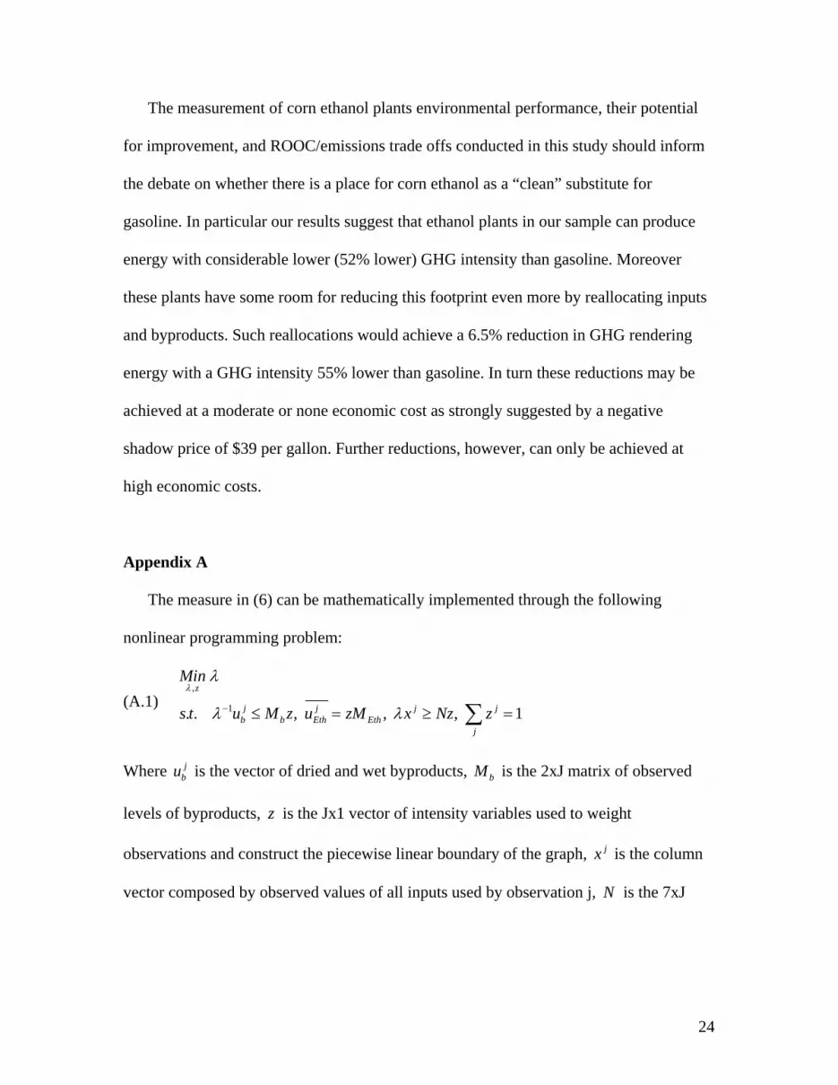
The measurement of corn ethanol plants environmental performance, their potential

for improvement, and ROOC/emissions trade offs conducted in this study should inform

the debate on whether there is a place for corn ethanol as a “clean” substitute for

gasoline. In particular our results suggest that ethanol plants in our sample can produce

energy with considerable lower (52% lower) GHG intensity than gasoline. Moreover

these plants have some room for reducing this footprint even more by reallocating inputs

and byproducts. Such reallocations would achieve a 6.5% reduction in GHG rendering

energy with a GHG intensity 55% lower than gasoline. In turn these reductions may be

achieved at a moderate or none economic cost as strongly suggested by a negative

shadow price of $39 per gallon. Further reductions, however, can only be achieved at

high economic costs.

Appendix A

The measure in (6) can be mathematically implemented through the following

nonlinear programming problem:

(A.1) ,

1

. . , , , 1

z

j j j jb b Eth Eth

j

Min

s t u M z u zM x Nz z

λλ

λ λ− ≤ = ≥ =∑

Where jbu is the vector of dried and wet byproducts, bM is the 2xJ matrix of observed

levels of byproducts, z is the Jx1 vector of intensity variables used to weight

observations and construct the piecewise linear boundary of the graph, jx is the column

vector composed by observed values of all inputs used by observation j, N is the 7xJ

25

matrix of observed values of inputs for all observations, and jEthu is the observed level of

ethanol production of the thj DMU.

After multiplying the constraints times λ it is easily seen that this is equivalent to the

following problem:

(A.2) ,

2

. . , , , , ,

z

j j j jb b Eth Eth

j

Min

s t u M z x Nz z u M z z zλ λ λ λ

′ΓΓ

′′ ′ ′ ′≤ Γ ≥ = = Γ = =∑

Following Färe et al. problem (A.1) is reformulated into problem (A.2) because the

only nonlinear constraint is an equality constraint (i.e. 2λ=Γ ) and is, hence, easier to

program. In particular, these sub vector hyperbolic measures of technical efficiency are

calculated through a nonlinear program implemented with the FMINCON procedure in

MATLAB.

Appendix B

The following program describes the problem:

(B.1) , ,

0.00668274 0.063015823 0.0007445

0.4197522186 0.407868

. . , z, ,

DDGS MWDGSc NG electx u u

DDGS MWDGS

jDDGS DDGS MWDGS MWDGS Eth Eth

Min GHG x x x

u u

s t u M z u M u M z x N

= + +

− −

≤ ≤ = ≥ , 1j

jz z =∑

Where DDGSu is the vector of dried byproducts, DDGSM is the 2xJ matrix of observed

levels of DDGS, z is JX1 vector of intensity variables, MWDGSu is the vector of modified

wet byproducts, MWDGSM is the 2xJ matrix of observed levels of MWDGS , x is the

vector of all inputs, and N is the 7xJ matrix of observed levels of inputs. This program

was calculated using the LINPROG routine in MATLAB.

26

Based on this quantity, we calculate overall environmental efficiency by solving for

jgE implicitly through Eq. (8) for each observation.

Appendix C

Proof:

Let us denote the vector of coefficients of Eq. (1) by ( ),xα β , where xα is the vector of

coefficients for corn, natural gas, and electricity, and β is the vector of coefficients for

both byproducts. In addition, let us define an arbitrary output and input vector by ( ),p bx u

where ( ), ,p c NG electx x x x= and ( ),b MWDGS DDGSu u u= and denote the thj DMU’s observed

output and input vector by ( ),j jp bx u .

Let ( ) ( )( )1, ,j j j j j

p b g g p b gx u GHG E x u E GR−

∈ , then ( ),p bx u GR∈ and since jgE is a

minimum:

( ) ( ) ( ) ( )( ) ( )

0.00668274 0.063015823 0.0007445

0.407868 / 0.4197522186 /

j j j j j jx p b g c g NG g elect

j j j jMWDGS g DDGS g

x u E x E x E x

u E u E

α β+ = + +

− −

Let us denote observations j’s minimum feasible GHG level by jGHG . There are three

cases to consider:

1. Assume ( ) jx p bx u GHGα β+ < , then ( ),p bx u GR∉

2. Asume ( ){ }jx p bx u GHGα β+ > , then

( ) ( ){ } ( ) ( ) ( ){ }, : , :jx x x p bv w v w GHG v w v w x uα β α β α β+ ≤ ⊆ + ≤ + and since the

hyperplanes defining the two sets are parallel, jgE can not be a minimum.

27

Cases 1 and 2 leave the following case:

3. ( ) jx p bx u GHGα β+ = . Therefore ( )1 jj j j j

g x p g bE x E u GHGα β−+ = .

Acknowledgements

Study supported by the Agricultural Research Service, University of Nebraska, and

USDA regional project NC506.

References

[1] Coelli, T., Lauwers, L., and Van Huylenbroeck, G. Environmental efficiency

measurement and the materials balance condition. Journal of Productivity

Analysis 2007; 28: 3-12.

[2] Eidman, Vernon R. Ethanol Economics of Dry Mill Plants. In Corn-Based Ethanol in

Illinois and the U.S.: A Report from the Department of Agricultural and

Consumer Economics, University of Illinois, 2007.

[3] Färe, R., S. Grosskopf and C.A.K. Lovell, Production Frontiers, Cambridge:

Cambridge University Press, 1994.

[4] Farrell, A. E., R. J. Plevin, B. T. Turner, A. D. Jones, M., O’Hare, and D. M.

Kammen.. Ethanol can contribute to energy and environmental goals. Science

2006; 311(5760): 506–508.

[5] Kwiatkowski, Jason R., Andrew J. McAloon, Frank Taylor and David B. Johnson.

Modeling the process and costs of fuel ethanol production by the corn dry-grind

process. Industrial Crops and Products 2006; 23: 288-296.

28

[6] Liska, A.J H.S. Yang, V. Bremer, T. Klopfenstein, D.T. Walters, G. Erickson, K.G.

Cassman. Improvements in Life Cycle energy Efficiency and greenhouse Gas

Emissions of Corn-Ethanol. Journal of Industrial Ecology 2009a; 13(1): 58-74.

[7] Liska, A.J H.S. Yang, V. Bremer, D.T. Walters, G. Erickson, T. Klopfenstein, D.

Kenney, P. Tracy, R. Koelsch, K.G. Cassman. BESS: Biofuel Energy Systems

Simulator; Life Cycle Energy and Emissions Analysis Model for Corn-Ethanol

Biofuel, 2009b; vers.2008.3.1. www.bess.unl.edu. University of Nebraska-

Lincoln.

[8] McAloon, Andrew, Frank Taylor and Winne Yee. Determining the Cost of Producing

Ethanol from Corn Starch and Lignocellulosic Feedstocks. National Renewable

Energy Laboratory, 2000; NREL/TP-580-28893.

[9] Perrin, R.K, Fretes, N, and Sesmero J.P. Efficiency in Midwest US Corn Ethanol

Plants: a Plant Survey. Energy Policy. 2009; 37, 4: 1309-1316

[10] Pimentel, David and Tad W. Patzek. Ethanol Production Using Corn, Switchgrass,

and Wood; Biodiesel Production Using Soybean and Sunflower. Natural

Resources Research, 2005; 14, 1: 65-76.

[11] Plevin, R J, and S Mueller. The effect of CO2 regulations on the cost of corn ethanol

production. Environmental Res. Lett. 2008; 3 024003 .

[12] Shapouri, Hosein and Paul Gallagher. USDA's 2002 Ethanol Cost-of-Production

Survey. Agricultural Economic Report No. 841, U.S. Dept of Agriculture, 2005.

[13] Wang, Michael, May Wu and Hong Huo. Life-cycle energy and greenhouse gas

emission impacts of different corn ethanol plant types. Environ. Res. Lett. 2007;

2.

29

Fig. 1 - Isopollution and Sets

Fig. 2 - Environmental Technical Efficiency

cx

jIso pollution− DDGSu

( ),j jc DDGSx u

jgGHG

( )DDGS cu f x=

( ), , jEthGR V S u

•A •B

BIso pollution−

Isopollution DDGSu

cx

( ),j jc DDGSx u

jgGHG ( )DDGS cu f x=

( ),GR V S

30

Fig. 3 - Decomposition of Overall Environmental Efficiency

Fig. 4 - Shadow Cost from GHG Minimizing to Profit Maximizing Allocation

jIso pollution− DDGSu

cx

( ),j jc DDGSx u

jgGHG

( )u f x=

( ),GR V S

•A • C

BIso pollution−

•B

DDGSu

• A

jGHG

•B

*jπ

jπ

*jGHG

cornx

31

-3500 -3000 -2500 -2000 -1500 -1000 -500 0 500 1000 15000

1

2

3

4

5

6

7

8

Shadow Values of GHG ($/ton)

Freq

uenc

y (n

umbe

r of o

bser

vatio

ns)

Fig. 5 - Histogram of Shadow Values (observed to ROOC-maximizing)

-1000 -800 -600 -400 -200 0 200 400 600 800 10000

1

2

3

4

5

6

Shadow Values of GHG ($/ton)

Freq

uenc

y (n

umbe

r of o

bser

vatio

ns)

Fig. 6 - Histogram of Shadow Values (observed to GHG-minimizing)

32

-2000 -1000 0 1000 2000 3000 4000 5000 60000

0.5

1

1.5

2

2.5

3

3.5

4

4.5

5

Shadow Values of GHG ($/ton)

Freq

uenc

y (n

umbe

r of o

bser

vatio

ns)

Fig. 7 – Histogram of Shadow Values (GHG Minimizing to Profit Maximizing)

Fig. 8 - ROOC and GHG

• ( ),j jGHG π • ( ),j jGHG π

( )* *,j jGHG π •

$1,726

-$39

- $466

ROOC

33

Table 1. Characteristics of the seven surveyed plants States

Represented Iowa, Michigan, Minnesota, Missouri, Nebraska, S. Dakota, Wisconsin

Annual

Production Rate (million

gal/year)

Smallest 42.5 Average 53.1

Largest 88.1

Number of

Survey Responses by

Quarters

03_2006 5 04_2006 6 01_2007 7 02_2007 7 03_2007 7 04_2007 2

Percent of Byproduct Sold

as Dry DGS

Smallest 0 Average 54 Largest 97

Primary Market

Technique

Corn Ethanol DDGS MWDGS Spot 0 0 3 1

Customer Contract 5 1 0 1 Third Party/Agent 0 5 2 2

Table 2. Descriptive Statistics: Inputs and Outputs

Corn

(million bushels)

Natural Gas (thousand

MMBTUs)

Electricity (million kwh)

Ethanol (million gallons)

DDGS (thousand

tons)

MWDGS (thousand

tons) Average 4.8 361 7,8 13.7 21.3 14.5 Std Dev 0.9 61 1.5 2.8 10 15.4

Min 3.6 297 6.7 10.6 0 0.2 Max 8 569 13.3 22,9 34.2 56.2

34

Table 3. Environmental Efficiency Decomposition

DMU Technical

Environmental Efficiency

Allocative Environmental

Efficiency

Overall Environmental

Efficiency

Reduction of GHG (tons)[a]

Reduction of GHG (%)[b]

1 0.977 0.983 0.961 3,268 6 2 1 0.931 0.931 6,227 11 3 0.985 0.970 0.956 3,617 7 4 1 0.951 0.951 3,801 7 5 1 0.993 0.993 567 1 6 0.979 0.993 0.973 2,331 4 7 1 0.948 0.948 4,697 9 8 1 0.947 0.947 4,704 8 9 1 1 1 0 0 10 0.997 0.959 0.956 3,539 7 11 1 0.989 0.989 950 2 12 1 1 1 0 0 13 1 0.940 0.940 8,007 9 14 1 0.949 0.949 4,625 9 15 1 0.944 0.944 4,804 9 16 1 0.974 0.974 2,015 4 17 1 0.985 0.985 1,098 2 18 1 0.938 0.938 5,178 10 19 1 0.987 0.987 1,133 2 20 1 1 1 0 0 21 1 0.947 0.947 4,611 9 22 1 0.967 0.967 2,736 5 23 1 0.974 0.974 2,023 4 25 1 0.985 0.985 1,199 2 26 1 0.970 0.970 2,614 5 27 1 1 1 0 0 28 1 0.917 0.917 7,941 14 29 1 0.956 0.956 3,708 7 30 1 0.961 0.961 3,068 6 31 1 0.964 0.964 2,831 6 32 0.993 0.980 0.973 2,239 4 33 1 0.992 0.992 684 1 34 1 0.914 0.914 8,662 14

Average 0.998 0.967 0.965 3,116 6

35

Table 4. Shadow Values of GHG: observed to profit maximizing combination

DMU WTP for change in

allocation, *j jπ π− ($)

Change in GHG emissions, *j jGHG GHG− (tons)

Shadow Value of GHG ($/ton)

1 948,565 -2,618 -362 2 1,483,022 -5,648 -263 3 2,094,972 -2,728 -768 4 1,223,985 -3,105 -394 5 619,562 120 5,147 - outlier 6 1,263,224 -1,920 -658 7 1,515,535 -4,100 -370 8 2,398,535 -4,405 -545 9 3,199 0 INFINITE 10 850,101 -2,636 -322 11 719,229 -264 -2,726 12 1,382 0 INFINITE 13 2,175,472 -7,709 -282 14 1,597,466 -4,026 -397 15 1,751,089 -4,339 -404 16 825,632 -1,027 -804 17 1,692 0 INFINITE 18 1,540,254 -4,555 -338 19 1,230,951 -488 -2,521 20 258,318 295 877 21 1,797,859 -3,726 -483 22 1,975,711 -2,035 -971 23 781,594 -344 -2,269 24 1,041,712 -332 -3,141 25 2,192,398 -1,990 -1,101 26 9,613 0 INFINITE 27 2,301,210 -7,495 -307 28 1,252,438 -3,075 -407 29 1,439,841 -2,291 -629 30 1,106,262 -1,801 -614 31 727,808 -1,367 -532 32 1,396,934 271 5,154 - outlier 33 1,865,307 -8,663 -215

Average 1,420,685 -3,052 -466 Median 1,439,841 -2,636 -546

36

Table 5. Reallocation from observed to profit maximizing combination Category

Measure Corn Natural Gas Electricity Dry Wet

Average Change (%) -5.88 -3.83 -0.41 26.03 -10.23

Table 6. Shadow Values of GHG: observed to GHG minimizing combination

DMU WTP for change in

allocation, j jEπ π− ($)

Change in GHG emissions, j j

EGHG GHG− (tons) Shadow Value of

GHG ($/ton) 1 659,193 -3,268 -202 2 443,897 -6,227 -71 3 134,209 -3,617 -37 4 -343,266 -3,801 90 5 286,956 -567 -506 6 -526,747 -2,331 226 7 294,875 -4,697 -63 8 610,737 -4,704 -130 9 -18,561 0 INFINITE 10 -886,553 -3,539 250 11 260,637 -950 -274 12 -817,158 0 INFINITE 13 1,728,919 -8,007 -216 14 432,472 -4,625 -94 15 -221,003 -4,804 46 16 -788,455 -2,015 391 17 -842,611 -1,098 767 18 1,041,500 -5,178 -201 19 326,317 -1,133 -288 20 -542,483 0 INFINITE 21 -417,870 -4,611 91 22 1,343,752 -2,736 -491 23 -373,408 -2,023 185 24 -839,949 -1,199 700 25 1,600,339 -2,614 -612 26 -263,194 0 INFINITE 27 307,697 -7,941 -39 28 176,556 -3,708 -48 29 164,586 -3,068 -54 30 -327,399 -2,831 116 31 -649,530 -2,239 290 32 -611,531 -684 894 33 1,046,320 -8,662 -121

Average 138,988 -3,548 -39 Median 176,556 -3,268 -54

37

Table 7. Reallocation from observed to GHG minimizing combination Category

Measure Corn Natural Gas Electricity Dry Wet Average Change (%) -3.05 -6.83 -1.35 -33.63 -4.11

Table 8. Shadow Values: GHG minimizing to profit maximizing combination

DMU WTP for change in

allocation, *j j

Eπ π− ($) Change in GHG emissions,

*j j

EGHG GHG− (tons) Shadow Value of

GHG ($/ton) 1 289,372 650 445 2 1,039,125 579 1,794 3 1,960,763 889 2,206 4 1,567,251 695 2,254 5 332,607 688 484 6 1,789,971 411 4,355 7 1,220,660 597 2,044 8 1,787,797 300 5,964 9 21,760 0 INFINITE

10 1,736,654 903 1,923 11 458,592 687 668 12 818,540 0 INFINITE 13 446,554 298 1,500 14 1,164,994 599 1,945 15 1,972,092 465 4,240 16 1,614,087 988 1,633 17 844,302 1,098 769 18 498,754 622 801 19 904,634 645 1,403 20 800,801 321 2,493 21 2,215,729 886 2,501 22 631,958 701 901 23 1,155,002 1,679 688 24 1,881,661 868 2,168 25 592,059 623 950 26 272,807 0 INFINITE 27 1,993,513 446 4,474 28 1,075,882 632 1,701 29 1,275,255 777 1,641 30 1,433,661 1,030 1,392 31 1,377,339 872 1,580 32 2,008,466 955 2,104 33 818,987 0 INFINITE

Average 1,243,777 721 1,726 Median 1,220,660 687 1,778

38

Table 9. Reallocation from GHG minimizing to profit-maximizing point Category

Measure Corn Natural Gas Electricity Dry Wet

Average Change (%) -2.75 2.82 0.94 12.45 -97.65