Epileptic seizure detection using dynamic wavelet network

Epileptic seizure detection using dynamic wavelet network

Abdulhamit Subasi*

Department of Electrical and Electronics Engineering, Kahramanmaras Sutcu Imam University, 46601 Kahramanmaras, Turkey

Abstract

Epileptic seizures are manifestations of epilepsy. Careful analyses of the electroencephalograph (EEG) records can provide valuable

insight and improved understanding of the mechanisms causing epileptic disorders. The detection of epileptiform discharges in the EEG is an

important component in the diagnosis of epilepsy. Wavelet transform is particularly effective for representing various aspects of non-

stationary signals such as trends, discontinuities, and repeated patterns where other signal processing approaches fail or are not as effective.

Through wavelet decomposition of the EEG records, transient features are accurately captured and localized in both time and frequency

context. This paper deals with a novel method of analysis of EEG signals using discrete wavelet transform, and classification using ANN.

EEG signals were decomposed into the frequency sub-bands using wavelet transform. Then these sub-band frequencies were used as an input

to an ANN with two discrete outputs: normal and epileptic. In this study, FEBANN and DWN based classifiers were developed and compared

in relation to their accuracy in classification of EEG signals. The comparisons between the developed classifiers were primarily based on

analysis of the ROC curves as well as a number of scalar performance measures pertaining to the classification. The DWN-based classifier

outperformed the FEBANN based counterpart. Within the same group, the DWN-based classifier was more accurate than the FEBANN-

based classifier.

q 2005 Elsevier Ltd. All rights reserved.

Keywords: Electroencephalogram (EEG); Epileptic seizure; Discrete wavelet transform (DWT); Feedforward error backpropagation artificial neural network

(FEBANN); Dynamic wavelet network (DWN)

1. Introduction

Epileptic seizures result from a temporary electrical

disturbance of the brain. Sometimes seizures may go

unnoticed, depending on their presentation, and sometimes

may be confused with other events, such as a stroke, which

can also cause falls or migraines. Approximately one in

every 100 persons will experience a seizure at some time in

their life (Iasemidis et al., 2003). Unfortunately, the

occurrence of an epileptic seizure seems unpredictable

and its process is very little understood. Electroencephalo-

gram (EEG) has been the most utilized signal to clinically

assess brain activities. EEG is a record of the electrical

potentials generated by the cerebral cortex nerve cells.

There are two different types of EEG depending on where

the signal is taken in the head: scalp or intracranial. For

scalp EEG, the focus of this research, small metal discs, also

0957-4174/$ - see front matter q 2005 Elsevier Ltd. All rights reserved.

doi:10.1016/j.eswa.2005.04.007

* Tel.: C90 344 219 1253; fax: C90 344 219 1052.

E-mail address: [email protected].

known as electrodes, are placed on the scalp with good

mechanical and electrical contact. Intracranial EEG is

obtained by special electrodes implanted in the brain during

a surgery. In order to provide an accurate detection of the

voltage of the brain neuron current, the electrodes of low

impedance (!5 kU). The changes in the voltage difference

between electrodes are sensed and amplified before being

transmitted to a computer program to display the tracing of

the voltage potential recordings. The recorded EEG

provides a continuous graphic exhibition of the spatial

distribution of the changing voltage fields over time.

Since routine clinical diagnosis needs to analysis of EEG

signals, some automation and computer techniques have

been used for this aim. In the early days of automatic EEG

processing, representations based on a Fourier transform

have been most commonly applied. This approach is based

on earlier observations that the EEG spectrum contains

some characteristic waveforms that fall primarily within

four frequency bands—d (!4 Hz), q (4–8 Hz), a (8–

13 Hz), and b (13–30 Hz). Such methods have proved

beneficial for various EEG characterizations, but fast

Fourier transform (FFT), suffer from large noise sensitivity.

Parametric power spectrum estimation methods such as

Expert Systems with Applications 29 (2005) 343–355

www.elsevier.com/locate/eswa

http://www.elsevier.com/locate/eswa

A. Subasi / Expert Systems with Applications 29 (2005) 343–355344

autoregressive (AR), reduces the spectral loss problems and

gives better frequency resolution. But, since the EEG

signals are non-stationary, the parametric methods are not

suitable for frequency decomposition of these signals

(Subasi, 2005).

A powerful method was proposed in the late 1980s to

perform time-scale analysis of signals: the wavelet trans-

forms (WT). This method provides a unified framework for

different techniques that have been developed for various

applications (Adeli, Zhou, &, Dadmehr, 2003; Basar,

Schurmann, Demiralp, Basar-Eroglu, & Ademoglu, 2001;

Folkers, Mosch, Malina, & Hofmann, 2003; Geva, &

Kerem, 1998; Hazarika, Chen, Tsoi, & Sergejer, 1997;

Kalayci, & Ozdamar, 1995; Khan, & Gotman, 2003;

Patwardhan, Dhawan, & Relue, 2003; Petrosian, Prokhorov,

Homan, Dashei, & Wunsch, 2000; Quiroga, Sakowitz,

Basar, & Schurmann, 2001; Quiroga, & Schurmann, 1999;

Rosso, Blanco, & Rabinowicz, 2003; Rosso, Martin, &

Plastino, 2002; Samar, Bopardikar, Rao, & Swartz, 1999;

Soltani, Simard, & Boichu, 2004; Zhang, Kawabata, & Liu,

2001). It should also be emphasized that the WT is

appropriate for analysis of non-stationary signals, and this

represents a major advantage over spectral analysis. Hence

the WT is well suited to locating transient events. Such

transient events as spikes can occur during epileptic

seizures.

Wavelet is an effective time–frequency analysis tool for

analyzing transient signals. Its feature extraction and

representation properties can be used to analyze various

transient events in biological signals. Adeli et al. (2003)

gave an overview of the DWT developed for recognizing

and quantifying spikes, sharp waves and spike-waves. They

used wavelet transform to analyze and characterize epilepti-

form discharges in the form of 3-Hz spike and wave

complex in patients with absence seizure. Through wavelet

decomposition of the EEG records, transient features are

accurately captured and localized in both time and

frequency context. The capability of this mathematical

microscope to analyze different scales of neural rhythms is

shown to be a powerful tool for investigating small-scale

oscillations of the brain signals. A better understanding of

the dynamics of the human brain through EEG analysis can

be obtained through further analysis of such EEG records.

Numerous other techniques from the theory of signal

analysis have been used to obtain representations and

extract the features of interest for classification purposes.

Neural networks and statistical pattern recognition methods

have been applied to EEG analysis. Neural network

detection systems have been proposed by a number of

researchers (Gabor, Leach, & Dowla, 1996; Haselsteiner, &

Pfurtscheller, 2000; Kiymik, Akin, & Subasi, in

press; Peters, Pfurtscheller, & Flyvbjerg, 2001; Pradhan,

Sadasivan, & Arunodaya, 1996; Qu, & Gotman, 1997;

Robert, Gaudy, & Limoge, 2002; Sun, & Sclabassi, 2000;

Webber, Lesser, Richardson , & Wilson, 1996; Weng, &

Khorasani, 1996).

Kalayci and Ozdamar (1995) showed that an ANN

performs better, if the input and output data can be

processed to capture the characteristic features of the signal.

They used a wavelet representation for automated detection

of the EEG spikes. More recently, ANN that applies

Bayesian methods are shown to be more robust compared

with other techniques because they incorporate measures of

confidence in their output for the Levenberg-Marquardt

(LM) procedure (Vuckovic, Radivojevic, Chen, & Popovic,

2002). In addition, standard MLP was improved by using

finite impulse response filters (FIR) instead of static weights

for a temporal processing of data (Haselsteiner, &

Pfurtscheller, 2000). Petrosian et al. (2000) showed that

the ability of specifically designed and trained recurrent

neural networks (RNN) combined with wavelet pre-

processing, to predict the onset of epileptic seizures both

on scalp and intracranial recordings. Recently, Kiymik et al.

(2004) presented time–frequency analysis of EEG signals

for detecting the information on alertness and drowsiness

using spectral densities of DWT coefficients as an input to

ANN.

Some studies, such as those of Petrosian et al. (2000),

report seizure prediction after analyzing one channel of

electroencephalogram (EEG) from an intracranial depth

electrode in one patient. In these studies, using univariate

techniques no analysis of baseline data far removed from the

seizure was undertaken. A potential pitfall of conclusions

based upon such limited data is that quantitative changes

identified prior to seizure onset may not be specific to the

pre-seizure period, but may occur at other times as well,

unrelated to epileptic events. Validation of prediction

algorithms on long, continuous sets of clinical data,

representing all states of awareness, is an important part

of more recent seizure prediction studies. A number of

promising quantitative features derived from the EEG, each

with different theoretical bases, have demonstrated utility

for seizure prediction.

As compared to the conventional method of frequency

analysis using Fourier transform or short time Fourier

transform, wavelets enable analysis with a coarse to fine

multi-resolution perspective of the signal (Subasi, 2005). In

this work, DWT has been applied for the time–frequency

analysis of EEG signals and ANN for the classification

using wavelet coefficients. EEG signals were decomposed

into frequency sub-bands using discrete wavelet transform

(DWT). An ANN based system was implemented to classify

the EEG signal to one of the categories: epileptic or normal.

The aim of this study was to develop a simple algorithm for

the detection of epileptic seizure which could also be

applied to real-time.

This paper aims to compare the more advanced and

relatively recent neural network techniques, as mathematical

tools for developing classifiers for the detection of epileptic

seizure. In the neural network techniques, both the feedfor-

ward error backpropagation ANN (FEBANN), and the

dynamic wavelet neural network (DWN) (Becerikli, 2004;

A. Subasi / Expert Systems with Applications 29 (2005) 343–355 345

Oysal, Yilmaz, & Koklukaya, 2005) will be used. The choice

of these two networks was based on the fact that the former is

the most popular type of ANNs and the latter is one of the

most powerful networks commonly used in solving

classification/discrimination problems. The accuracy of the

various classifiers will be assessed and cross-compared, and

advantages and limitations of each technique will be

discussed.

Table 1

Frequencies corresponding to different levels of decomposition for

Daubechies 4 filter wavelet with a sampling frequency of 200 Hz

Decomposed signal Frequency range (Hz)

D1 50–100

D2 25–50

D3 12.5–25

D4 6.25–12.5

D5 3.125–6.25

A5 0–3.125

2. Materials and method

2.1. Subjects and data recording

The EEG data used in our study was downloaded from

24-h EEG recorded from both epileptic patients and normal

subjects. The following bipolar EEG channels were selected

for analysis: F7-C3, F8-C4, T5-O1 and T6-O2. In order to

assess the performance of the classifier, we selected 500

EEG segments containing spike and wave complex,

artifacts, and background normal EEG. Twenty absence

seizures (petit mal) from 5 epileptic patients admitted for

video-EEG monitoring were analyzed. The subjects con-

sisted of 3 males and 2 females, age 28.87G15.27 (meanGSD; range 6–43) with a diagnosis of epilepsy and no other

accompanying disorders. Recordings were done under video

control to have an accurate determination of the different

stage of the seizure. The different stages of EEG signals

were determined by two physicians. EEG data were

acquired with Ag/AgCl disk electrodes placed using the

10–20 international electrode placement system. The

recordings band-pass filtered (1–70 Hz) EEG. For this

study, 15-min, 4 channel recordings containing epileptiform

events (spikes, spike and waves) were digitized at 200

samples per second using 12 bit resolution. All EEG were

taken during restful wakefulness stage but some portions of

the EEG contained EMG artifacts.

2.2. Visual inspection and validation

Two neurologists with experience in the clinical analysis

of EEG signals separately inspected every recording

included in this study to score epileptic and normal signals.

Each event was filed on the computer memory and linked to

the tracing with its start and duration. These were then

revised by the two experts jointly to solve disagreements

and set up the training set for the program, consenting to

the choice of threshold for the epileptic seizure detection.

The agreement between the two experts was evaluated—for

the testing set—as the rate between the numbers of epileptic

seizures detected by both experts. A further step was then

performed with the aim of checking the disagreements and

setting up a ‘gold standard’ reference set (De Carli, Nobili,

Gelcich, & Ferrillo, 1999). When revising this unified event

set, the human experts, by mutual consent, marked each

state as epileptic or normal. They also reviewed each

recording entirely for epileptic seizures that had been

overlooked by all during the first pass and marked them as

definite or possible. This validated set provided the

reference evaluation to estimate the sensitivity and speci-

ficity of computer scorings. Nevertheless, a preliminary

analysis was carried out solely on events in the training set,

as each stage in these sets had a definite start and duration.

2.3. Analysis using discrete wavelet transforms

The Discrete Wavelet Transform (DWT) is a versatile

signal processing tool that finds many engineering and

scientific applications. One area in which the DWT has been

particularly successful is the epileptic seizure detection

because it captures transient features and localizes them in

both time and frequency content accurately.

DWT analyzes the signal at different frequency bands,

with different resolutions by decomposing the signal into a

coarse approximation and detail information. DWT

employs two sets of functions called scaling functions and

wavelet functions, which are associated with low-pass and

high-pass filters, respectively. The decomposition of the

signal into the different frequency bands is simply obtained

by successive high-pass and low-pass filtering of the time

domain signal. Detailed derivations related to wavelet

transform are given in Appendix.

Selection of suitable wavelet and the number of levels of

decomposition is very important in analysis of signals using

DWT. The typical way is to visually inspect the data first,

and if the data are kind of discontinuous, Haar or other sharp

wavelet functions are applied; otherwise a smoother wavelet

can be employed. Usually, tests are performed with different

types of wavelets and the one which gives maximum

efficiency is selected for the particular application.

The number of levels of decomposition is chosen based

on the dominant frequency components of the signal. The

levels are chosen such that those parts of the signal that

correlate well with the frequencies required for classifi-

cation of the signal are retained in the wavelet coefficients.

Since the EEG signals do not have any useful frequency

components above 30 Hz, the number of levels was chosen

to be 5. Thus the signal is decomposed into the details D1–

D5 and one final approximation, A5. The ranges of various

frequency bands are shown in Table 1.

0 500 1000 1500 2000 2500 3000–500

0

500

Am

plitu

de

0 500 1000 1500 2000 2500 3000–500

0

500

Am

plitu

de

0 500 1000 1500 2000 2500 3000–500

0

500

Am

plitu

deA

mpl

itude

0 500 1000 1500 2000 2500 3000–500

0

500

F8-C4

F7-C3

T6-O2

T5-O1

Fig. 1. EEG signal taken from unhealthy subject (epileptic patient).


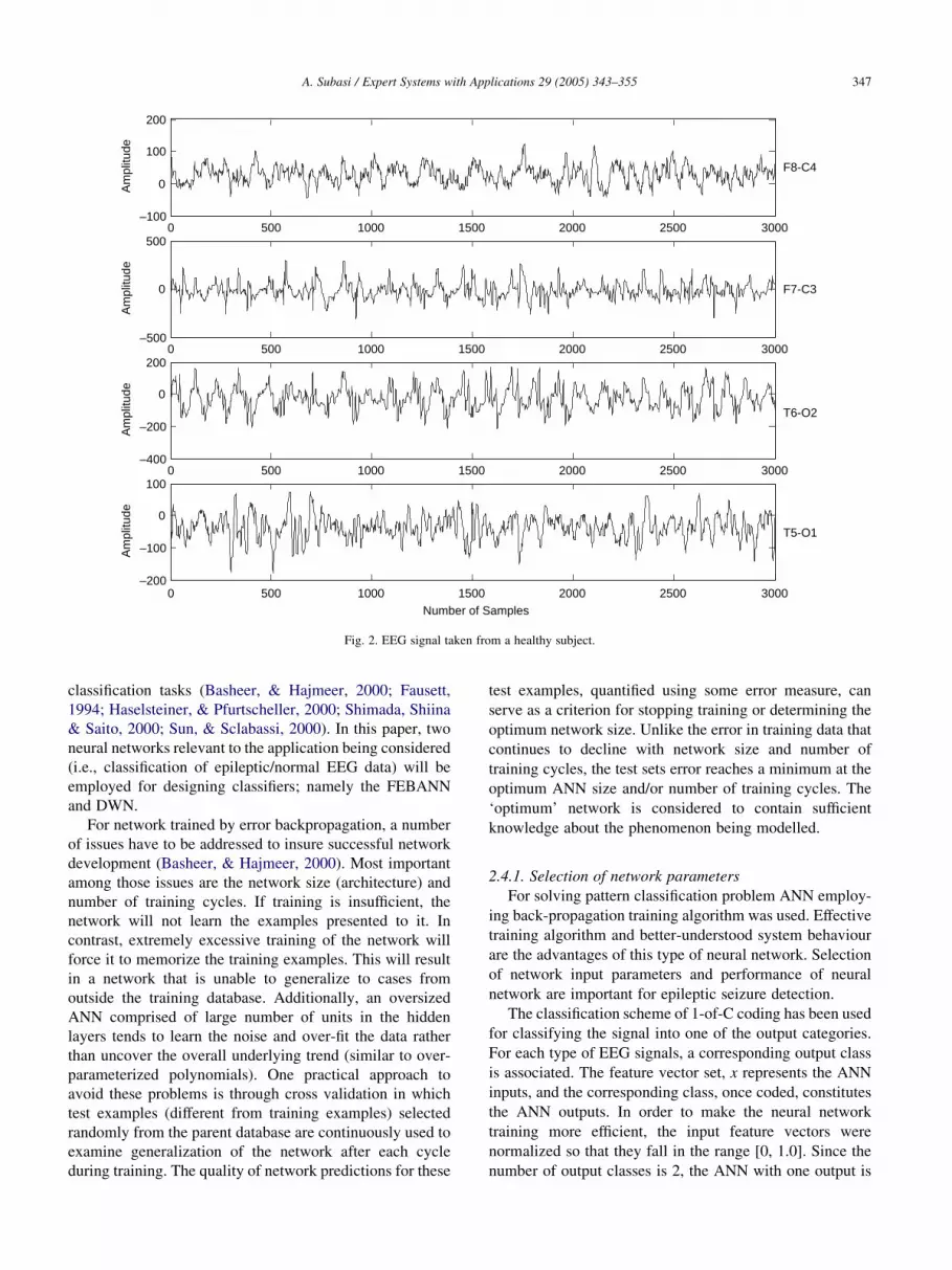
The proposed method was applied on a wide variety of

EEG data for both epileptic and normal signals. Four

channels of EEG (F7-C3, F8-C4, T5-O1 and T6-O2)

recorded from a patient with absence seizure epileptic

discharges are shown in Fig. 1 and normal EEG signal

shown in Fig. 2. Fig. 3 shows five different levels of

approximation (identified by A1–A5 and displayed in the

left column) and details (identified by D1–D5 and displayed

in the right column) of an epileptic EEG signal. Fig. 4 shows

five different levels of approximation (identified by A1–A5

and displayed in the left column) and details (identified by

D1–D5 and displayed in the right column) of a normal EEG

signal. These approximation and detail records are recon-

structed from the Daubechies 4 (DB4) wavelet filter. These

approximation and detail records are reconstructed from the

wavelet coefficients. Approximation A4 is obtained by

superimposing details D5 on approximation A5. Approxi-

mation A3 is obtained by superimposing details D4 on

approximation A4, and so on. Finally, the original signal is

obtained by superimposing details D1 on approximation A1.

Wavelet transform acts like a mathematical microscope,

zooming into small scales to reveal compactly spaced

events in time and zooming out into large scales to exhibit

the global waveform patterns (Adeli et al., 2003).

The extracted wavelet coefficients provide a compact

representation that shows the energy distribution of the EEG

signal in time and frequency. Table 1 presents frequencies

corresponding to different levels of decomposition for

Daubechies order 4 wavelet with a sampling frequency of

200 Hz. It can be seen from Table 1 that the components A5

decomposition are within the d (1–4 Hz), D5 decomposition

are within the q range (4–8 Hz), D4 decomposition are

within the a range (8–13 Hz), and D3 decomposition are

within the b range (13–30 Hz). Lower level decompositions

corresponding to higher frequencies have negligible mag-

nitudes in a normal EEG.

2.4. Classification using artificial neural networks

Artificial neural networks (ANNs) are formed of cells

simulating the low level functions of biological neurons. In

ANN, knowledge about the problem is distributed in

neurons and connections weights of links between neurons.

The neural network has to be trained to adjust the

connection weights and biases in order to produce the

desired mapping. At the training stage, the feature vectors

are applied as input to the network and the network adjusts

its variable parameters, the weights and biases, to capture

the relationship between the input patterns and outputs.

ANNs are particularly useful for complex pattern recog-

nition and classification tasks. The capability of learning

from examples, the ability to reproduce arbitrary non-linear

functions of input, and the highly parallel and regular

structure of ANN make them especially suitable for pattern

0 500 1000 1500 2000 2500 3000–100

0

100

200A

mpl

itude

0 500 1000 1500 2000 2500 3000–500

0

500

Am

plitu

de

0 500 1000 1500 2000 2500 3000–400

–200

0

200

Am

plitu

de

0 500 1000 1500 2000 2500 3000–200

–100

0

100

Number of Samples

Am

plitu

de

F8-C4

F7-C3

T6-O2

T5-O1

Fig. 2. EEG signal taken from a healthy subject.


classification tasks (Basheer, & Hajmeer, 2000; Fausett,

1994; Haselsteiner, & Pfurtscheller, 2000; Shimada, Shiina

& Saito, 2000; Sun, & Sclabassi, 2000). In this paper, two

neural networks relevant to the application being considered

(i.e., classification of epileptic/normal EEG data) will be

employed for designing classifiers; namely the FEBANN

and DWN.

For network trained by error backpropagation, a number

of issues have to be addressed to insure successful network

development (Basheer, & Hajmeer, 2000). Most important

among those issues are the network size (architecture) and

number of training cycles. If training is insufficient, the

network will not learn the examples presented to it. In

contrast, extremely excessive training of the network will

force it to memorize the training examples. This will result

in a network that is unable to generalize to cases from

outside the training database. Additionally, an oversized

ANN comprised of large number of units in the hidden

layers tends to learn the noise and over-fit the data rather

than uncover the overall underlying trend (similar to over-

parameterized polynomials). One practical approach to

avoid these problems is through cross validation in which

test examples (different from training examples) selected

randomly from the parent database are continuously used to

examine generalization of the network after each cycle

during training. The quality of network predictions for these

test examples, quantified using some error measure, can

serve as a criterion for stopping training or determining the

optimum network size. Unlike the error in training data that

continues to decline with network size and number of

training cycles, the test sets error reaches a minimum at the

optimum ANN size and/or number of training cycles. The

‘optimum’ network is considered to contain sufficient

knowledge about the phenomenon being modelled.

2.4.1. Selection of network parameters

For solving pattern classification problem ANN employ-

ing back-propagation training algorithm was used. Effective

training algorithm and better-understood system behaviour

are the advantages of this type of neural network. Selection

of network input parameters and performance of neural

network are important for epileptic seizure detection.

The classification scheme of 1-of-C coding has been used

for classifying the signal into one of the output categories.

For each type of EEG signals, a corresponding output class

is associated. The feature vector set, x represents the ANN

inputs, and the corresponding class, once coded, constitutes

the ANN outputs. In order to make the neural network

training more efficient, the input feature vectors were

normalized so that they fall in the range [0, 1.0]. Since the

number of output classes is 2, the ANN with one output is

500 1000 1500 2000 2500 3000

–400–200

0200400

Original signal and approximations

s

0 1000 2000 3000–1000

0

1000

A1

A2

A3

A4

A5

D1

D2

D3

D4

D5

0 1000 2000 3000–1000

0

1000

0 1000 2000 3000–1000

0

1000

0 1000 2000 3000–1000

0

1000

0 1000 2000 3000–1000

0

1000

Number of Samples

500 1000 1500 2000 2500 3000

–100

0

100

Details

500 1000 1500 2000 2500 3000

–200

0

200

500 1000 1500 2000 2500 3000

–400–200

0200

500 1000 1500 2000 2500 3000–400–200

0200

400

500 1000 1500 2000 2500 3000

–400–200

0200

Number of Samples

Fig. 3. Approximate and detailed coefficients of EEG signal taken from unhealthy subject (epileptic patient).


sufficient to produce a code for each class. The outputs are

represented by basis vectors:

[0.1]Znormal

[0.9]Zepileptic

Each dummy variable is given the value 0.1 except for

the one corresponding to the correct category, which is

given the value 0.9. Using target values of 0.1 and 0.9

instead of the common practice of 0 and 1 prevents the

outputs of the network from being directly interpretable as

posterior probabilities (Kandaswamy, Kumar, Ramanathan,

Jayaraman, & Malmurugan, 2004).

2.4.2. Cross validation

Cross validation (CV) (Basheer, & Hajmeer, 2000;

Haselsteiner, & Pfurtscheller, 2000) is often used for

comparing two or more learning ANN models to estimate

which model will perform the best on the problem at hand.

With n-fold CV, the available data is partitioned into n

disjoint subsets, the union of which is equal to the original

set. Each learning model is trained on nK1 of the available

subsets, and then tested on the one subset which was not

used during training. This process is repeated n times, each

time using a different test set chosen from the n available

partitions of the training data, until all possible choices for

the test set have been exhausted. The n test set scores for

each learning model are then averaged, and the model with

the highest average test set score is chosen as the one most

likely to perform well on unseen data (Kandaswamy et al.,

2004).

2.4.3. Measuring error

Given a random set of initial weights, the outputs of the

network will be very different from the desired classifi-

cations. As the network is trained, the weights of the system

are continually adjusted to reduce the difference between

the output of the system and the desired response. The

difference is referred to as the error and can be measured in

several ways. The most common measurement is sum

500 1000 1500 2000 2500 3000

0

50

100

Original signal and approximations

0 1000 2000 3000–200

0

200

0 1000 2000 3000–200

0

200

0 1000 2000 3000–200

0

200

0 1000 2000 3000–200

0

200

0 1000 2000 3000–100

0

100

Number of Samples

500 1000 1500 2000 2500 3000–5

0

5

Details

500 1000 1500 2000 2500 3000–10

0

10

500 1000 1500 2000 2500 3000

–20

0

20

500 1000 1500 2000 2500 3000

–20

0

20

500 1000 1500 2000 2500 3000–40–20

0204060

Number of Samples

sA

1A

2A

3A

4A

5

D1

D2

D3

D4

D5

Fig. 4. Approximate and detailed coefficients of EEG signal taken from a healthy subject.


squared error (SSE) and mean squared error (MSE). SSE is

the average of the squares of the difference between each

output and the desired output (Basheer, & Hajmeer, 2000;

Haselsteiner, & Pfurtscheller, 2000). In this study, SSE was

used for measuring performance of the neural network.

W2

W3

u y

W1

Fig. 5. Schematic diagram of a DWN with three-wavelon.

2.5. Dynamic wavelet network

Dynamic wavelet network (DWN) models have been

used in the meaning of a network. The DWN model we used

has unconstrained connectivity and has dynamic elements in

the wavelon (neuron of DWN) processing units. A

schematic diagram for the dynamic networks with three

neurons is shown in Fig. 5. Wi can be a wavelon in a DWN.

In general, there are L input signals which can be time-

varying, n dynamic units, n bias terms, and M output signals.

The units have dynamics associated with them and they

receive the input from themselves, the bias term, and from

all other units. The output of a unit yi is an activation

function h(xi) of a state variable xi associated with the unit.

The output of the overall network is a linear weighted sum

of the unit outputs. The bias term bi is added to the unit

inputs. pij is the input connection weights from the jth input

to the ith wavelon, wij is the interconnection weight from the

jth wavelon to the ith wavelon and qij is the output

connection weight from the jth wavelon to the ith output. Ti

is the dynamic constant of the ith wavelon and bi is the bias

(or polarization) term of the ith wavelon (Becerikli, 2004).

In DWNs, wavelet neurons (wavelons) input over a lag

dynamic transport to output via a wavelet activation

function. Wavelets are usually explained as basis functions

which are compact (closed and bounded), orthogonal


(or orthonormal), and have time–frequency localization

properties. But, to provide all of those properties is very

difficult. Basis functions are called ‘activation functions’ in

ANN literature, and can be a global or local feature in time.

Global basis functions are active for the wide values of

inputs and the receptive field of the basis function is

approximately constant far from the center (i.e., logarithmic

sigmoid function). But, the local basis functions are only

active near the center; the value tends to zero far from the

centre (Becerikli, 2004).

If the global basis function is used in a network, all

activation functions interact with each other and each node,

and they cover a wide input interval. This causes the large

number of parameters to adjust and necessitates a long

computation time. In addition, for wide input intervals,

much more extrapolation error occurs. The most important

disadvantage of orthonormal compact basis functions is that

they can not be obtained in the closed analytical form.

To remove all those disadvantages, the local basis

functions can be used. The local basis functions are only

active for certain inputs. In addition, the generalization

errors decrease (Becerikli, 2004). In this study, only the

local basis functions have been used. The most important

local function is Gaussian:

fðtÞ Z exp Kt2

2

� �; x2R (1)

where f2L2(R). For the more general case:

ft Kb

a

� �Z exp K

1

2

t Kb

a

� �2� �; t 2R (2)

where b is the center or translation and a is the standard

deviation or dilation. However, the Gaussian function is not

local in frequency (Becerikli, 2004). The locality features in

both time and frequency is a very important concept for the

representation of the signals. Therefore, the mission of the

wavelet functions is comprehensive.

The locality in time and frequency can be explained as

follows:

†
If a function is described in a bounded interval and has a
very small value outside the boundary, then that function

is local in time. The local function in time can be shifted

by changing its centre.

†
If the frequency spectrum of the local function in time is
described in a bounded frequency interval and has very

small value outside the boundary, and also can be shifted

by changing its dilation, then that function is local in

frequency.

A deficiency of Gaussian-based ANNs is that they do not

have localization capabilities in frequency. Since the

Gaussian function is not local in frequency, it is very

difficult to use Gaussian-based functions in some appli-

cations (Sanner, & Slotine, 1992). To overcome these

problems, there is a very effective way to use wavelet

functions with time–frequency localization properties

(Cannon, & Slotine, 1995). In some studies, the first

derivative of the Gaussian function has been used (Mallat,

1987; Qussar, Rivals, Personnaz, & Dreyfus, 1998).

However, the locality properties of the second derivative

of the Gaussian function are clearer. A non-orthonormal

Mexican Hat basis function (second derivative of the

Gaussian function) can be easily written in the analytical

form and its Fourier transform can be found (Becerikli,

2004), thus:

fðtiÞ Z ð1 K t2i Þexp K

t2i

2

� �; t 2R (3)

fðuÞ Zffiffiffiffiffiffi2p

pu2 exp K

u2

2

� �; u2R (4)

where u is a real frequency. The last equation can be

generalized as follows:

fti Kbi

ai

� �Z 1 K

ti Kbi

ai

� �2� �exp K

1

2

ti Kbi

ai

� �2� �

(5)

where bi and ai are the translation (center) and dilation

(standard deviation) parameters, respectively. Wavelet

functions have efficient time–frequency localization proper-

ties, as shown from the frequency spectrum (Mallat, 1987).

If the dilation parameter is changed, the support region

width of the wavelet function changes, but the number of

cycles does not change. That is, the peak number does not

change; however, when the dilation parameter decreases,

the peak point of the spectrum shifts to a higher frequency.

Therefore, all frequency spectrums can be obtained by

changing the dilation. In this study, Eq. (4) has been used as

a mother (main) wavelet (Becerikli, 2004). An N-dimen-

sional mother wavelet can be given in the separable

structure with the product rule as follows (Cannon, &

Slotine, 1995; Mallat, 1987; Qussar et al., 1998; Zhang, &

Benveniste, 1992; Zhang, Walter, & Lee, 1995):

FiðtÞ ZYN

jZ1

fj

tj Kbij

aij

� �(6)

where ti2RN is the input and N is the input number. A

function yZf(t) can be represented with wavelets obtained

from the mother wavelet, (Cannon, & Slotine, 1995; Mallat,

1987; Qussar et al., 1998) as below:

yi Z hiðtÞ ZXNw

jZ1

sijfjðtÞCai0 CXN

jZ1

aiktk (7)

where sij are the coefficients of the mother wavelets, Nw is

the number of wavelets, ai0 is a mean or bias term, and aik

are the linear term coefficients of this approach.


The wavelet function in this structure will be used in the

DWN given in Fig. 5. The structure used in (Becerikli,

2004; Becerikli, Konar, & Samad, 2003; Becerikli, Oysal, &

Konar, 2004; Oysal et al., 2005) has been adapted to this

network. The wavelets in Eqs. (6) and (7) will be used as the

activation functions in the network. Each activation

function has a single input/single output (SISO), and can

be re-expressed as:

FiðtiÞ Z fi

ti Kbij

aij

� �(8)

yi Z hiðtiÞ ZXNw

jZ1

sijfi

ti Kbij

aij

� �Cai0 Cai1ti (9)

fi

ti Kbij

aij

� �Z 1 K

ti Kbij

aij

� �2� �exp K

1

2

ti Kbij

aij

� �2� �

(10)

2.6. Evaluation of performance

The coherence of the diagnosis of the expert neurologists

and diagnosis information was calculated at the output of

the classifier. Prediction success of the classifier may be

evaluated by examining the confusion matrix. In order to

analyze the output data obtained from the application,

sensitivity (true positive ratio) and specificity (true negative

ratio) are calculated by using confusion matrix. The

sensitivity value (true positive, same positive result as the

diagnosis of expert neurologists) was calculated by dividing

the total of diagnosis numbers to total diagnosis numbers

that are stated by the expert neurologists. Sensitivity, also

called the true positive ratio, is calculated by the formula:

Sensitivity Z TPR ZTP

TP CFN!100% (11)

On the other hand, specificity value (true negative, same

diagnosis as the expert neurologists) is calculated by

dividing the total of diagnosis numbers to total diagnosis

numbers that are stated by the expert neurologists.

Specificity, also called the true negative ratio, is calculated

by the formula:

Specifity Z TNR ZTN

TN CFP!100% (12)

Neural network analyses were compared to each other by

receiver operating characteristic (ROC) analysis. ROC

analysis is an appropriate means to display sensitivity and

specificity relationships when a predictive output for two

possibilities is continuous. In its tabular form, the ROC

analysis displays true and false positive and negative totals

and sensitivity and specificity for each listed cutoff value

between 0 and 1 (Subasi, in 2005).

In order to perform the performance measure of the

output classification graphically, the ROC curve was

calculated by analyzing the output data obtained from the

test. Furthermore, the performance of the model may be

measured by calculating the region under the ROC curve.

The ROC curve is a plot of the true positive rate (sensitivity)

against the false positive rate (1-specificity) for each

possible cutoff. A cutoff value is selected that may classify

the degree of epileptic seizure detection correctly by

determining the input parameters optimally according to

the used model.

3. Results and discussion

In this study, we used EEG signals of normal and

epileptic patients in order to perform comparison between

two neural network models. EEG recordings were divided

into sub-band frequencies such as a, b, d and q by using

DWT (Figs. 3 and 4). Then these wavelet sub-band

frequencies d (1–4 Hz), q (4–8 Hz), a (8–13 Hz) and b

(13–30 Hz) are applied to neural networks.

The classification efficiency which is defined as the

percentage ratio of the number of EEG signals correctly

classified to the total number of EEG signals considered for

classification also depends on the type of wavelet chosen for

the application. In the previous work on application of WT

in EEG analysis (Subasi, 2005), Daubechies wavelet of

order 2 (db2) was used and found to yield good results. In

order to investigate the effect of other wavelets on

classifications efficiency, tests were carried out using other

wavelets also. Apart from db2, Symmlet of order 10

(sym10), Coiflet of order 4 (coif4), Daubechies of order 4

(db4) and Daubechies of order 8 (db8) were also tried.

Average efficiency obtained for each wavelet when EEG

signals were classified using various ANN structures. It can

be seen that the Daubechies wavelet offers better efficiency

than the others, and db4 is marginally better than db2 and

db8. Hence db4 wavelet is chosen for this application.

3.1. Development of neural network model

The objective of the modelling phase in this application

was to develop classifiers that are able to identify any input

combination as belonging to either one of the two classes:

normal or epileptic. For developing neural network

classifiers, 300 examples were randomly taken from the

500 examples and used for training the neural networks, and

100 for the cross validation. The remaining 100 examples

were kept aside and used for testing the developed models.

The class distribution of the samples in the training and

validation data set is summarized in Table 2.

The ANNs were designed with wavelet sub-band

frequencies of EEG signal using DWT, in the input layer;

and the output layer consisted of one node representing

whether epileptic seizure detected or not. A value of 0.1 was

used when the experimental investigation indicated a

normal and 0.9 for epileptic seizure. The preliminary

Table 2

Class distribution of the samples in the training and the validation data sets

Class Training set Validation

set

Test set Total

Epileptic 102 46 42 190

Normal 198 54 58 310

Total 300 100 100 500

Table 3

Comparison of neural network models for EEG signals

Classifier

type

Correctly

classified

(%)

Specifity

(%)

Sensitivity

(%)

Area under

ROC curve

FEBANN 91 91.3 90.4 0.907

DWN 93 93.1 92.8 0.921


architecture of the network was examined using one and two

hidden layers with a variable number of hidden nodes in

each. It was found that one hidden layer is adequate for the

problem at hand. Thus the sought network will contain three

layers of nodes. The training procedure started with one

hidden node in the hidden layer, followed by training on the

training data, and then by testing on the validation data to

examine the network’s prediction performance on cases

never used in its development. Then, the same procedure

was run repeatedly each time the network was expanded by

adding one more node to the hidden layer, until the best

architecture and set of connection weights were obtained.

Using the modified error-backpropagation algorithm for

training, a training rate of 0.0001 and momentum coefficient

of 0.95 were found optimum for training the network with

various topologies. The selection of the optimal network

was based on monitoring the variation of error and some

accuracy parameters as the network was expanded in the

hidden layer size and for each training cycle. The sum of

squares of error representing the sum of square of deviations

of ANN solution (output) from the true (target) values for

both the training and test sets was used for selecting the

optimal network. Additionally, because the problem

involves classification into two classes, sensitivity and

specifity were used as a performance measure. A computer

program that we have written for the training algorithm

based on backpropagation of error was used to develop the

FEBANNs.

The classifier implemented for this work is a DWN with

one hidden layer and one output layer. An input vector is

applied to the input layer where all of the inputs are

distributed to each unit in the first hidden layer. All of the

units have weight vectors which are multiplied by these

input vectors. Each unit sums these inputs and produces a

value that is transformed by a wavelet activation function.

The output of the final layer is then computed by

multiplying the output vector from the hidden layer by the

weights into the final layer. More summations and

activations at these units then give the actual output of the

network. We used a network with a variable number of

hidden units and one output unit as in FEBANN. One output

unit is all that is needed because we are only classifying a

two-task problem.

The number of input vector was equal to the total number

of wavelet coefficients of four sub-bands (a, b, d, q), and the

number of output vector consisted of one node representing

whether epileptic seizure detected or not. Optimum number

of neurons in the hidden layer, training algorithm,

parameters of the training algorithm, and the activation

functions of the two layers were determined by repeated

simulation. According to the theory, the number of nodes in

the hidden layer of the network is equal to that of wavelet

base. If the number is too small, DWN may not reflect the

complex function relationship between input data and

output value. On the contrary, a large number may create

such a complex network that might lead to a very large

output error caused by over-fitting of the training sample.

The optimum number of nodes in hidden layer is 65. As a

result, the network in this paper is constructed by the error

backpropagation neural network using Mexican Hat wavelet

basic function as node activation function. The amount by

which the weights are adjusted on each step is parameter-

ized by learning rate constants. We used one learning rate

for the hidden layer and a different rate for the output layer.

After trying a large number of different values, we found

that a learning rate of 0.0001 for the hidden layer and the

output layer produced the best performance.

3.2. Experimental results

Firstly we used sub-band frequencies of EEG signals for

FEBANN and DWN classification. The procedure was

repeated on EEG recordings of all subjects (healthy and

epileptic patients). Table 3 shows a summary of the

performance measures by using sub-band frequencies of

EEG signals using DWT. It is obvious from Table 3 that the

DWN-based classifier is ranked first in terms of its correct

classification percentage of the EEG signals (epileptic/-

normal data 93%), while the FEBANN-based classifier

came second (91%). While the FEBANN classified the same

data with a success rate of 90.4% and DWN classified the

same data with a success rate of 92.8%.

Also, the area under ROC curves for two classifiers

(FEBANN and DWN) are given in Table 3. To quantify the

performance characteristics of each classifier, the area under

ROC curve (AUC) was computed for validation data ROC

curve. Table 3 presents a summary of these AUC values for

the 2 classifiers developed. As can be seen from Table 3, the

DWN-based classifier is undoubtedly the better classifier

with AUCZ0.921 for the validation data ROC curves,

while the FEBANN-based classifier exhibited a slightly

lower performance (AUCZ0907).

The testing performance of the DWN diagnostic system

is found to be satisfactory and we think that this system can


be used in clinical studies in the future after it is developed.

This application brings objectivity to the evaluation of EEG

signals and its automated nature makes it easy to be used in

clinical practice. Besides the feasibility of a real-time

implementation of the expert diagnosis system, diagnosis

may be made more accurately by increasing the variety and

the number of parameters. A ‘black box’ device that may be

developed as a result of this study may provide feedback to

the neurologists for classification of the EEG signals quickly

and accurately by examining the EEG signals with real-time

implementation.

4. Summary and conclusions

Diagnosing epilepsy is a difficult task requiring obser-

vation of the patient, an EEG, and gathering of additional

clinical information. An artificial neural network that

classifies subjects as having or not having an epileptic

seizure provides a valuable diagnostic decision support tool

for physicians treating potential epilepsy, since differing

etiologies of seizures result in different treatments.

Conventional method of classification of EEG signals

using mutually exclusive time and frequency domain

representations does not give efficient results. In this

work, a novel method of diagnostic classification of EEG

signals is proposed. The EEG signals were decomposed into

time–frequency representations using DWT. FEBANN and

DWN were implemented for the classification of EEG

signals using DWT sub-bands as inputs.

In this paper, two approaches to develop classifiers for

identifying epileptic seizure were discussed. One approach

is based on the traditional neural network technology,

mainly using feedforward neural network trained by the

error-backpropagation algorithm (FEBANN) and the other

is the dynamic wavelet network (DWN). Using DWT of

EEG signals, two classifiers; namely FEBANN, and DWN,

were constructed and cross-compared in terms of their

accuracy relative to the observed epileptic/normal patterns.

The comparisons were based on analysis of the receiving

operator characteristic (ROC) curves of the three classifiers

and two scalar performance measures derived from the

confusion matrices; namely specifity and sensitivity. The

DWN-based classifier identified accurately all the epileptic

and normal cases with specifity 93.1% and sensitivity 92.8%

and the FEBANN-based classifier with specifity 91.3% and

sensitivity 90.4%. Out of the 100 epileptic/normal cases,

FEBANN-based classifier misclassified 9 cases, while the

DWN-based classifier misclassified 7 cases.

Essentially, DWNs and FEBANNs require deciding on

the number of hidden layers, number of nodes in each

hidden layer, number of training iteration cycles, choice of

activation function, selection of the optimal learning rate

and momentum coefficient, as well as other parameters and

problems pertaining to convergence of the solution.

Advantages of DWNs over FEBANNs include their

robustness to noisy data (with outliers) which can severely

hamper many types of ANNs as well as most traditional

statistical methods. Finally, the fact that a DWN-based

classifier can be developed quickly makes such classifiers

efficient tools that can be easily re-trained, as additional data

become available, when implemented in the hardware of

EEG signal processing systems.

With specificity and sensitivity values both above 92%,

the wavelet neural network classification may be used as an

important diagnostic decision support mechanism to assist

physicians in the treatment of epileptic patients.

Appendix

Wavelet transform

The wavelet transform specifically permits to discrimi-

nation of non-stationary signals with different frequency

features (Daubechies, 1996). A signal is stationary if it does

not change much over time. Fourier transform can be

applied to the stationary signals. However, like EEG, plenty

of signals may contain non-stationary or transitory charac-

teristics. Thus it is not ideal to directly apply Fourier

transform to such signals.

The wavelet transform decomposes a signal into a set of

basic functions called wavelets. These basic functions are

obtained by dilations, contractions and shifts of a unique

function called wavelet prototype. Continuous wavelets are

functions generated from one single function j by dilations

and translations (Cohen, & Kovacevic, 1996; Rioul, &

Vetterli, 1991).

ja;bðtÞ Z1ffiffiffiffiffiffi

aj jp j

t Kb

a

� �(A.1)

where b is real valued and called the shift parameter. The

function set (ja,b(t)) is called a wavelet family. Since the

parameters (a, b) are continuous valued, the transform is

called continuous wavelet transform. The definition of

classical wavelets as dilates of one function means that high

frequency wavelets correspond to a!1 or narrow width,

while low frequency wavelets have aO1 or wider width. In

the wavelet transform, f(t) is expressed as linear combi-

nation of scaling and wavelet functions. Both scaling

functions and the wavelet functions are complete sets

(Rioul, & Vetterli, 1991). However, it is common to employ

both wavelet and scaling functions in the transform

representation. In general, the scale and shift parameters

of the discreet wavelet family are given by

a Z aj0; b Z kb0a

j0 (A.2)

where j and k are integers. The function family with

discretized parameters becomes

jj;kðtÞ Z aKj=20 j aKjt Kkb0

� �(A.3)


jj,k(t) is called the discrete wavelet transform (DWT) basis.

Although it is called DWT, the time variable of the

transform is still continuous. The DWT coefficients of a

continuous time function are similarly defined as

dj;k Z hfwðtÞ;jj;kðtÞi Z1

aj=20

ðfwðtÞjða

Kj0 t Kkb0Þdt (A.4)

When the DWT set (jj,k(t)) is complete, the wavelet

representation of a function fw(t) is expressed as

fwðtÞ ZX

j

Xk

hfwðtÞ;jj;kðtÞijj;kðtÞ (A.5)

In general, a function can be completely represented by

using L-finite resolutions of wavelet, and the scaling

function with parameters value of a0Z2 and b0Z1 as

fwðtÞ ZXN

kZKN

cL;k2KL=2fð2t=L KkÞ

CXL

jZ1

XN

kZKN

dj;k2Kj=2jð2t=j KkÞ (A.6)

Where scaling coefficients [cL,k] are similarly defined as

cL;k Z hfwðtÞ;fL;KðtÞi Z

ðfwðtÞ2

KL=2ft

2LKk

�dt (A.7)

and

fL;kðtÞ Z 2KL=2fð2KLt KkÞ (A.8)

j Z 2X

k

h1ðtÞfð2t KkÞ (A.9)

f Z 2X

k

h0ðkÞfð2t KkÞ (A.10)

References

Adeli, H., Zhou, Z., & Dadmehr, N. (2003). Analysis of EEG records in an

epileptic patient using wavelet transform. Journal of Neuroscience

Methods, 123, 69–87.

Basar, E., Schurmann, M., Demiralp, T., Basar-Eroglu, C., & Ademoglu, A.

(2001). Event-related oscillations are ‘real brain responses’—wavelet

analysis and new strategies. International Journal of Psychophysiology,

39, 91–127.

Basheer, I. A., & Hajmeer, M. (2000). Artificial neural networks:

Fundamentals, computing, design, and application. Journal of Micro-

biological Methods, 43, 3–31.

Becerikli, Y. (2004). On three intelligent systems: Dynamic neural, fuzzy

and wavelet networks for training trajectory. Neural Computing

Applications, 13(4), 339–351.

Becerikli, Y., Konar, A. F., & Samad, T. (2003). Intelligent optimal control

with dynamic neural networks. Neural Networks, 16(2), 251–259.

Becerikli, Y., Oysal, Y., & Konar, A. F. (2004). Trajectory priming with

dynamic fuzzy networks in nonlinear optimal control. IEEE Trans-

actions Neural Networks, 15(2), 383–394.

Cannon, M., & Slotine, J. J. E. (1995). Space-frequency localized basis

function networks for nonlinear system estimation and control.

Neurocomputing, 9(3), 293–342.

Cohen, A., & Kovacevic, J. (1996). Wavelets: the mathematical back-

ground. Proceedings of the IEEE, 84, 514–522.

Daubechies, I. (1996). Where do wavelets come from? A personal point of

view. Proceedings of the IEEE, 84, 510–513.

De Carli, F., Nobili, L., Gelcich, P., & Ferrillo, F. (1999). A method for the

automatic detection of arousals during sleep. Sleep, 22, 561–572.

Fausett, L. (1994). Fundamentals of neural networks architectures,

algorithms, and applications. Englewood Cliffs, NJ: Prentice Hall Inc..

Folkers, A., Mosch, F., Malina, T., & Hofmann, U. G. (2003). Realtime

bioelectrical data acquisition and processing from 128 channels

utilizing the wavelet-transformation. Neurocomputing, 52–54, 247–

254.

Gabor, A. J., Leach, R. R., & Dowla, F. U. (1996). Automated seizure

detection using a self-organizing neural network. Electroencephalo-

graphy and Clinical Neurophysiology, 99, 257–266.

Geva, A. B., & Kerem, D. H. (1998). Forecasting generalized epileptic

seizures from the EEG signal by wavelet analysis and dynamic

unsupervised fuzzy clustering. IEEE Transactions on Biomedical

Engineering, 45(10), 1205–1216.

Haselsteiner, E., & Pfurtscheller, G. (2000). Using time-dependent neural

networks for EEG classification. IEEE Transactions on Rehabilitation

Engineering, 8, 457–463.

Hazarika, N., Chen, J. Z., Tsoi, A. C., & Sergejew, A. (1997). Classification

of EEG signals using the wavelet transform. Signal Processing, 59(1),

61–72.

Iasemidis, L. D., Shiau, D. S., Chaovalitwongse, W., Sackellares, J. C.,

Pardalos, P. M., Principe, J. C., et al. (2003). Adaptive epileptic seizure

prediction system. IEEE Transactions on Biomedical Engineering,

50(5), 616–627.

Kalayci, T., & Ozdamar, O. (1995). Wavelet preprocessing for automated

neural network detection of EEG spikes. IEEE Engineering in Medicine

and Biology Magazine, Mar/Apr, 160–166.

Kandaswamy, A., Kumar, C. S., Ramanathan, R. P., Jayaraman, S., &

Malmurugan, N. (2004). Neural classification of lung sounds using

wavelet coefficients. Computers in Biology and Medicine, 34(6),

523–537.

Khan, Y. U., & Gotman, J. (2003). Wavelet based automatic seizure

detection in intracerebral electroencephalogram. Clinical Neurophy-

siology, 114, 898–908.

Kiymik, M. K., Akin, M., & Subasi, A. (2004). Automatic recognition of

alertness level by using wavelet transform and artificial neural network.

Journal of Neuroscience Methods, 139(2), 231–240.

Mallat, S. G. (1987). Multifrequency channel decompositions of images

and wavelet models. IEEE Transactions on ASSP, 37(12), 2091–2109.

Oysal, Y., Yilmaz, A.S., Koklukaya, E. (2005). A dynamic wavelet network

based adaptive load frequency control in power systems. Electrical

Power and Energy Systems, 27, 21–29.

Patwardhan, S. V., Dhawan, A. P., & Relue, P. A. (2003). Classification of

melanoma using tree structured wavelet transforms. Computer Methods

and Programs in Biomedicine, 72, 223–239.

Peters, B. O., Pfurtscheller, G., & Flyvbjerg, H. (2001). Automatic

differentiation of multichannel EEG signals. IEEE Transactions on

Biomedical Engineering, 48, 111–116.

Petrosian, A., Prokhorov, D., Homan, R., Dashei, R., & Wunsch, D. (2000).

Recurrent neural network based prediction of epileptic seizures in intra-

and extracranial EEG. Neurocomputing, 30, 201–218.

Pradhan, N., Sadasivan, P. K., & Arunodaya, G. R. (1996). Detection of

seizure activity in EEG by an artificial neural network: A preliminary

study. Computers and Biomedical Research, 29, 303–313.

Qu, H., & Gotman, J. (1997). A patient-specific algorithm for the detection

of seizure onset in long-term EEG monitoring: Possible use as a

warning device. IEEE Transactions on Biomedical Engineering, 44,

115–122.


Quiroga, R. Q., Sakowitz, O. W., Basar, E., & Schurmann, M. (2001).

Wavelet transform in the analysis of the frequency composition of

evoked potentials. Brain Research Protocols, 8, 16–24.

Quiroga, R. Q., & Schurmann, M. (1999). Functions and sources of event-

related EEG alpha oscillations studied with the wavelet transform.

Clinical Neurophysiology, 110, 643–654.

Qussar, Y., Rivals, I., Personnaz, L., & Dreyfus, G. (1998). Training

wavelet networks for nonlinear dynamic input–output modeling.

Neurocomputing, 20, 173–188.

Rioul, O., & Vetterli, M. (1991). Wavelet and signal processing. IEEE

Signal Processing Magazine , 14–46.

Robert, C., Gaudy, J. F., & Limoge, A. (2002). Electroencephalogram

processing using neural networks. Clinical Neurophysiology, 113,

694–701.

Rosso, O. A., Blanco, S., & Rabinowicz, A. (2003). Wavelet analysis of

generalized tonic-clonic epileptic seizures. Signal Processing, 83,

1275–1289.

Rosso, O. A., Martin, M. T., & Plastino, A. (2002). Brain electrical activity

analysis using wavelet-based informational tools. Physica A, 313, 587–

608.

Samar, V. J., Bopardikar, A., Rao, R., & Swartz, K. (1999). Wavelet

analysis of neuroelectric waveforms: A conceptual tutorial. Brain and

Language, 66, 7–60.

Sanner, R., & Slotine, J. J. E. (1992). Gaussian networks for direct adaptive

control. IEEE Transactions Neural Network, 13(6), 837–863.

Shimada, T., Shiina, T., & Saito, Y. (2000). Detection of characteristic

waves of sleep EEG by neural network analysis. IEEE Transactions on


Soltani, S., Simard, P., & Boichu, D. (2004). Estimation of the self-

similarity parameter using the wavelet transform. Signal Processing,

84, 117–123.

Subasi, A. (2005). Automatic recognition of alertness level from EEG by

using neural network and wavelet coefficients. Expert Systems with

Applications, 28, 701–711.

Sun, M., & Sclabassi, R. J. (2000). The forward EEG solutions can be

computed using artificial neural networks. IEEE Transactions on


Vuckovic, A., Radivojevic, V. A., Chen, C. N., & Popovic, D. (2002).

Automatic recognition of alertness and drowsiness from EEG by an

artificial neural network. Medical Engineering and Physics, 24,

349–360.

Webber, W. R. S., Lesser, R. P., Richardson, R. T., & Wilson, K. (1996).

An approach to seizure detection using an artificial neural network

(ANN). Electroencephalography and Clinical Neurophysiology, 98,

250–272.

Weng, W., & Khorasani, K. (1996). An adaptive structure neural network

with application to EEG automatic seizure detection. Neural Networks,

9, 1223–1240.

Zhang, Q., & Benveniste, A. (1992). Wavelet networks. IEEE Transactions

Neural Networks, 3(6), 889–898.

Zhang, M., Kawabata, H., & Liu, Z. Q. (2001). Electroencephalogram

analysis using fast wavelet transform. Computers in Biology and

Medicine, 31, 429–440.

Zhang, J., Walter, G. G., & Lee, W. (1995). Wavelet neural networks for

function learning. IEEE Transactions Signal Processing, 43(6), 1485–

1497.

Documents

Epileptic seizure detection using dynamic wavelet network