Embed Size (px)
Citation preview
Essential MATLABfor Engineers and Scientists

Essential MATLABfor Engineers and Scientists
Sixth Edition
Brian H. Hahn
Daniel T. Valentine
AMSTERDAM • BOSTON • HEIDELBERG • LONDONNEW YORK • OXFORD • PARIS • SAN DIEGO
SAN FRANCISCO • SINGAPORE • SYDNEY • TOKYO
Academic Press is an imprint of Elsevier
Academic Press is an imprint of Elsevier50 Hampshire Street, 5th Floor, Cambridge, MA 02139, United States525 B Street, Suite 1800, San Diego, CA 92101-4495, United StatesThe Boulevard, Langford Lane, Kidlington, Oxford OX5 1GB, United Kingdom125, London Wall, EC2Y, 5AS, United Kingdom
Copyright © 2017, 2013, 2010 Daniel T. Valentine. Published by Elsevier Ltd. All rights reserved.
Copyright © 2007, 2006, 2002 Brian D. Hahn and Daniel T. Valentine. Published by Elsevier Ltd.
MATLAB® is a trademark of The MathWorks, Inc. and is used with permission.The MathWorks does not warrant the accuracy of the text or exercises in this book.This book’s use or discussion of MATLAB® software or related products does not constitute endorsementor sponsorship by The MathWorks of a particular pedagogical approach or particular use of theMATLAB® software.
No part of this publication may be reproduced, stored in a retrieval system, or transmitted in any formor by any means, electronic, mechanical, photocopying, recording, or otherwise, without the priorwritten permission of the publisher.
Permissions may be sought directly from Elsevier’s Science & Technology Rights Department in Oxford,UK: phone: (+44) 1865 843830, fax: (+44) 1865 853333, E-mail: [email protected]. You mayalso complete your request online via the Elsevier homepage (http://www.elsevier.com), by selecting“Support & Contact” then “Copyright and Permission” and then “Obtaining Permissions.”
Library of Congress Cataloging-in-Publication DataA catalog record for this book is available from the Library of Congress.
British Library Cataloguing-in-Publication DataA catalogue record for this book is available from the British Library.
ISBN: 978-0-08-100877-5
For information on all Academic Press publicationsvisit our website at https://www.elsevierdirect.com
Publisher: Todd Green
Acquisition Editor: Stephen Merken
Editorial Project Manager: Nate McFadden
Production Project Manager: Stalin Viswanathan
Designer: Matthew Limbert
Typeset by VTeX
Preface
The main reason for a sixth edition of Essential MATLAB for Engineers and Scien-tists is to keep up with MATLAB, now in its latest version (9.0 Version R2016a).Like the previous editions, this one presents MATLAB as a problem-solvingtool for professionals in science and engineering, as well as students in thosefields, who have no prior knowledge of computer programming.
In keeping with the late Brian D. Hahn’s objectives in previous editions, thesixth edition adopts an informal, tutorial style for its “teach-yourself” ap-proach, which invites readers to experiment with MATLAB as a way of discov-ering how it works. It assumes that readers have never used this tool in theirtechnical problem solving.
MATLAB, which stands for “Matrix Laboratory,” is based on the concept ofthe matrix. Because readers will be unfamiliar with matrices, ideas and con-structs are developed gradually, as the context requires. The primary audiencefor Essential MATLAB is scientists and engineers, and for that reason certain ex-amples require some first-year college math, particularly in Part II. However,these examples are self-contained and can be skipped without detracting fromthe development of readers’ programming skills.
MATLAB can be used in two distinct modes. One, in keeping the modern-agecraving for instant gratification, offers immediate execution of statements (orgroups of statements) in the Command Window. The other, for the more pa-tient, offers conventional programming by means of script files. Both modesare put to good use here: The former encouraging cut and paste to take fulladvantage of Windows’ interactive environment. The latter stressing program-ming principles and algorithm development through structure plans.
Although most of MATLAB’s basic (“essential”) features are covered, this bookis neither an exhaustive nor a systematic reference. This would not be in keep-ing with its informal style. For example, constructs such as for and if are notalways treated, initially, in their general form, as is common in many texts, butare gradually introduced in discussions where they fit naturally. Even so, they xv
xvi Preface
are treated thoroughly here, unlike in other texts that deal with them only su-perficially. For the curious, helpful syntax and function quick references can befound in the appendices.
The following list contains other highlights of Essential MATLAB for Engineersand Scientists, Sixth Edition:
� Warnings of the many pitfalls that await the unwary beginner� Numerous examples taken from science and engineering (simulation, pop-
ulation modeling, numerical methods) as well as business and everydaylife
� An emphasis on programming style to produce clear, readable code� Comprehensive chapter summaries� Chapter exercises (answers and solutions to many of which are given in an
appendix)� A thorough, instructive index
Essential MATLAB is meant to be used in conjunction with the MATLAB soft-ware. The reader is expected to have the software at hand in order to workthrough the exercises and thus discover how MATLAB does what it is com-manded to do. Learning any tool is possible only through hands-on expe-rience. This is particularly true with computing tools, which produce correctanswers only when the commands they are given and the accompanying datainput are correct and accurate.
ACKNOWLEDGMENTS
I would like to thank Mary, Clara, Zoe Rae and Zach T. for their support andencouragement. I dedicate the sixth edition of Essential MATLAB for Engineersand Scientists to them.
Daniel T. Valentine

1P A R T
Essentials
Part 1 concerns those aspects of MATLAB that you need to know in order tocome to grips with MATLAB’s essentials and those of technical computing. Be-cause this book is a tutorial, you are encouraged to use MATLAB extensivelywhile you go through the text.
CONTENTS
Using MATLAB ...... 5Arithmetic ................. 5Variables.................... 7Mathematicalfunctions.................... 8Functions andcommands................. 8Vectors....................... 9Linear equations ...... 11Tutorials and demos 12
The desktop ......... 13Using the Editor andrunning a script ....... 13Help, publish andview ......................... 16Symbolics and theMuPAD notebookAPP.......................... 18Other APPS.............. 23Additional features .. 23
Sample program. 25Cut and paste .......... 25Saving a program:script files................ 27Current directory....... 28Running a script fromthe current folderbrowser .................... 29A program in action . 29
CHAPTER 1
Introduction
THE OBJECTIVES OF THIS CHAPTER ARE:
� To enable you to use some simple MATLAB commands from theCommand Window.
� To examine various MATLAB desktop and editing features.� To learn some of the new features of the MATLAB R2016a Desktop.� To learn to write scripts in the Editor and Run them from the Editor.� To learn some of the new features associated with the tabs (in particular,
the PUBLISH and APPS features).
MATLAB is a powerful technical computing system for handling scientific andengineering calculations. The name MATLAB stands for Matrix Laboratory, be-cause the system was designed to make matrix computations particularly easy.A matrix is an array of numbers organized in m rows and n columns. An exam-ple is the following m × n = 2 × 3 array:
A =(
1 3 52 4 6
)
Any one of the elements in a matrix can be plucked out by using the rowand column indices that identify its location. The elements in this exampleare plucked out as follows: A(1,1) = 1, A(1,2) = 3, A(1,3) = 5, A(2,1) = 2,A(2,2) = 4, A(2,3) = 6. The first index identifies the row number counted fromtop to bottom; the second index is the column number counted from left toright. This is the convention used in MATLAB to locate information in an array.A computer is useful because it can do numerous computations quickly, sooperating on large numerical data sets listed in tables as arrays or matrices ofrows and columns is quite efficient.
This book assumes that you have never used a computer before to do the sortof scientific calculations that MATLAB handles, but are able to find your way
3Essential MATLAB for Engineers and Scientists. DOI:10.1016/B978-0-08-100877-5.00002-5Copyright © 2017 Daniel T. Valentine. Published by Elsevier Ltd. All rights reserved.
Summary .............. 30
Exercises ...............31
Supplementarymaterial .................31
4 CHAPTER 1: Introduction
around a computer keyboard and know your operating system (e.g., Windows,UNIX or MAC-OS). The only other computer-related skill you will need issome very basic text editing.
One of the many things you will like about MATLAB (and that distinguishesit from many other computer programming systems, such as C++ and Java) isthat you can use it interactively. This means you type some commands at thespecial MATLAB prompt and get results immediately. The problems solved inthis way can be very simple, like finding a square root, or very complicated, likefinding the solution to a system of differential equations. For many technicalproblems, you enter only one or two commands—MATLAB does most of thework for you.
There are three essential requirements for successful MATLAB applications:
� You must learn the exact rules for writing MATLAB statements and usingMATLAB utilities.
� You must know the mathematics associated with the problem you want tosolve.
� You must develop a logical plan of attack—the algorithm—for solving aparticular problem.
This chapter is devoted mainly to the first requirement: learning some basicMATLAB rules. Computer programming is a precise science (some would alsosay an art); you have to enter statements in precisely the right way. There is asaying among computer programmers: Garbage in, garbage out. It means that ifyou give MATLAB a garbage instruction, you will get a garbage result.
With experience, you will be able to design, develop and implement compu-tational and graphical tools to do relatively complex science and engineeringproblems. You will be able to adjust the look of MATLAB, modify the way youinteract with it, and develop a toolbox of your own that helps you solve prob-lems of interest. In other words, you can, with significant experience, customizeyour MATLAB working environment.
As you learn the basics of MATLAB and, for that matter, any other computertool, remember that applications do nothing randomly. Therefore, as you useMATLAB, observe and study all responses from the command-line operationsthat you implement, to learn what this tool does and does not do. To beginan investigation into the capabilities of MATLAB, we will do relatively simpleproblems that we know the answers because we are evaluating the tool and itscapabilities. This is always the first step. As you learn about MATLAB, you arealso going to learn about programming, (1) to create your own computationaltools, and (2) to appreciate the difficulties involved in the design of efficient,robust and accurate computational and graphical tools (i.e., computer pro-grams).
1.1 Using MATLAB 5
In the rest of this chapter we will look at some simple examples. Don’t beconcerned about understanding exactly what is happening. Understanding willcome with the work you need to do in later chapters. It is very important foryou to practice with MATLAB to learn how it works. Once you have graspedthe basic rules in this chapter, you will be prepared to master many of thosepresented in the next chapter and in the Help files provided with MATLAB.This will help you go on to solve more interesting and substantial problems.In the last section of this chapter you will take a quick tour of the MATLABdesktop.
1.1 USING MATLAB
Either MATLAB must be installed on your computer or you must have accessto a network where it is available. Throughout this book the latest version atthe time of writing is assumed (Version R2016a).
To start from Windows, double-click the MATLAB icon on your Windows desk-top. To start from UNIX, type matlab at the operating system prompt. To startfrom MAC-OS open X11 (i.e., open an X-terminal window), then type mat-lab at the prompt. The MATLAB desktop opens as shown in Figure 1.1. Thewindow in the desktop that concerns us for now is the Command Window,where the special >> prompt appears. This prompt means that MATLAB iswaiting for a command. You can quit at any time with one of the followingways:
� Click the X (close box) in the upper right-hand corner of the MATLAB desk-top.
� Type quit or exit at the Command Window prompt followed by pressingthe ‘enter’ key.
Starting MATLAB automatically creates a folder named MATLAB in the user’sDocuments Folder. This feature is quite convenient because it is the defaultworking folder. It is in this folder that anything saved from the CommandWindow will be saved. Now you can experiment with MATLAB in the Com-mand Window. If necessary, make the Command Window active by placingthe cursor in the Command Window and left-clicking the mouse button any-where inside its border.
1.1.1 ArithmeticSince we have experience doing arithmetic, we want to examine if MATLABdoes it correctly. This is a required step to gain confidence in any tool and inour ability to use it.
Type 2+3 after the >> prompt, followed by Enter (press the Enter key) asindicated by <Enter>:
>> 2+3 <Enter>
6 CHAPTER 1: Introduction
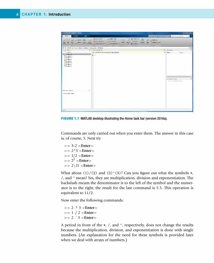
FIGURE 1.1 MATLAB desktop illustrating the Home task bar (version 2016a).
Commands are only carried out when you enter them. The answer in this caseis, of course, 5. Next try
>> 3-2 <Enter>>> 2*3 <Enter>>> 1/2 <Enter>>> 23 <Enter>>> 2\11 <Enter>
What about (1)/(2) and (2)^(3)? Can you figure out what the symbols *,/, and ^ mean? Yes, they are multiplication, division and exponentiation. Thebackslash means the denominator is to the left of the symbol and the numer-ator is to the right; the result for the last command is 5.5. This operation isequivalent to 11/2.
Now enter the following commands:
>> 2 .* 3 <Enter>>> 1 ./ 2 <Enter>>> 2 .ˆ 3 <Enter>
A period in front of the *, /, and ^, respectively, does not change the resultsbecause the multiplication, division, and exponentiation is done with singlenumbers. (An explanation for the need for these symbols is provided laterwhen we deal with arrays of numbers.)
1.1 Using MATLAB 7
Here are hints on creating and editing command lines:
� The line with the >> prompt is called the command line.� You can edit a MATLAB command before pressing Enter by using various
combinations of the Backspace, Left-arrow, Right-arrow, and Del keys.This helpful feature is called command-line editing.
� You can select (and edit) commands you have entered using Up-arrow andDown-arrow. Remember to press Enter to have the command carried out(i.e., to run or to execute the command).
� MATLAB has a useful editing feature called smart recall. Just type the first fewcharacters of the command you want to recall. For example, type the charac-ters 2* and press the Up-arrow key—this recalls the most recent commandstarting with 2*.
How do you think MATLAB would handle 0/1 and 1/0? Try it. If you insiston using ∞ in a calculation, which you may legitimately wish to do, type thesymbol Inf (short for infinity). Try 13+Inf and 29/Inf.
Another special value that you may meet is NaN, which stands for Not-a-Number. It is the answer to calculations like 0/0.
1.1.2 VariablesNow we will assign values to variables to do arithmetic operations with thevariables. First enter the command (statement in programming jargon) a = 2.The MATLAB command line should look like this:
>> a = 2 <Enter>
The a is a variable. This statement assigns the value of 2 to it. (Note that thisvalue is displayed immediately after the statement is executed.) Now try enter-ing the statement a = a + 7 followed on a new line by a = a * 10. Do youagree with the final value of a? Do we agree that it is 90?
Now enter the statement
>> b = 3; <Enter>
The semicolon (;) prevents the value of b from being displayed. However, bstill has the value 3, as you can see by entering without a semicolon:
>> b <Enter>
Assign any values you like to two variables x and y. Now see if you can assignthe sum of x and y to a third variable z in a single statement. One way of doingthis is
>> x = 2; y = 3; <Enter>>> z = x + y <Enter>
8 CHAPTER 1: Introduction
Notice that, in addition to doing the arithmetic with variables with assignedvalues, several commands separated by semicolons (or commas) can be puton one line.
1.1.3 Mathematical functionsMATLAB has all of the usual mathematical functions found on a scientific-electronic calculator, like sin, cos, and log (meaning the natural logarithm).See Appendix B.5 for many more examples.
� Find√
π with the command sqrt(pi). The answer should be 1.7725. Notethat MATLAB knows the value of pi because it is one of its many built-infunctions.
� Trigonometric functions like sin(x) expect the argument x to be in radians.Multiply degrees by π/180 to get radians. For example, use MATLAB to cal-culate sin(90◦). The answer should be 1 (sin(90*pi/180)).
� The exponential function ex is computed in MATLAB as exp(x). Use thisinformation to find e and 1/e (2.7183 and 0.3679).
Because of the numerous built-in functions like pi or sin, care must be takenin the naming of user-defined variables. Names should not duplicate thoseof built-in functions without good reason. This problem can be illustrated asfollows:
>> pi = 4 <Enter>>> sqrt(pi) <Enter>>> whos <Enter>>> clear pi <Enter>>> whos <Enter>>> sqrt(pi) <Enter>>> clear <Enter>>> whos <Enter>
Note that clear executed by itself clears all local variables in the workspace;>>clear pi clears the locally defined variable pi. In other words, if you de-cide to redefine a built-in function or command, the new value is used! Thecommand whos is executed to determine the list of local variables or com-mands presently in the workspace. The first execution of the command pi = 4in the above example displays your redefinition of the built-in pi: a 1-by-1 (or1x1) double array, which means this data type was created when pi was assigneda number (you will learn more about other data types later, as we proceed inour investigation of MATLAB).
1.1.4 Functions and commandsMATLAB has numerous general functions. Try date and calendar for starters.It also has numerous commands, such as clc (for clear command window). helpis one you will use a lot (see below). The difference between functions and
1.1 Using MATLAB 9
commands is that functions usually return with a value (e.g., the date), whilecommands tend to change the environment in some way (e.g., clearing thescreen or saving some statements to the workspace).
1.1.5 VectorsVariables such as a and b that were used in Section 1.1.2 above are called scalars;they are single-valued. MATLAB also handles vectors (generally referred to asarrays), which are the key to many of its powerful features. The easiest wayof defining a vector where the elements (components) increase by the sameamount is with a statement like
>> x = 0 : 10; <Enter>
That is a colon (:) between the 0 and the 10. There is no need to leave a spaceon either side of it, except to make it more readable. Enter x to check that xis a vector; it is a row vector—consisting of 1 row and 11 columns. Type thefollowing command to verify that this is the case:
>> size(x) <Enter>
Part of the real power of MATLAB is illustrated by the fact that other vectorscan now be defined (or created) in terms of the just defined vector x. Try
>> y = 2 .* x <Enter>>> w = y ./ x <Enter>
and
>> y = sin(x) <Enter>
(no semicolons). Note that the first command line creates a vector y by multi-plying each element of x by the factor 2. The second command line is an arrayoperation, creating a vector w by taking each element of y and dividing it bythe corresponding element of x. Since each element of y is two times the cor-responding element of x, the vector w is a row vector of 11 elements all equalto 2. Finally, z is a vector with sin(x) as its elements.
To draw a reasonably nice graph of sin(x), simply enter the following com-mands:
>> x = 0 : 0.1 : 10; <Enter>>> z = sin(x); <Enter>>> plot(x,z), grid <Enter>
The graph appears in a separate figure window. To draw the graph of the sinefunction illustrated in Figure 1.2 replace the last line above with
>> plot(x,y,’-rs’,’LineWidth’,2,’MarkerEdgeColor’,’k’,’MarkerSize’,5),grid<Enter>
10 CHAPTER 1: Introduction
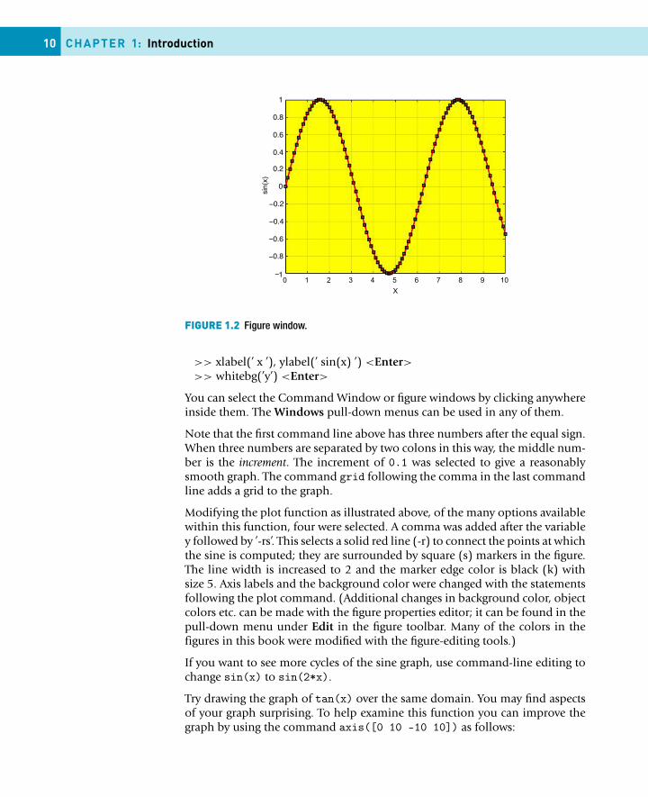
FIGURE 1.2 Figure window.
>> xlabel(’ x ’), ylabel(’ sin(x) ’) <Enter>>> whitebg(’y’) <Enter>
You can select the Command Window or figure windows by clicking anywhereinside them. The Windows pull-down menus can be used in any of them.
Note that the first command line above has three numbers after the equal sign.When three numbers are separated by two colons in this way, the middle num-ber is the increment. The increment of 0.1 was selected to give a reasonablysmooth graph. The command grid following the comma in the last commandline adds a grid to the graph.
Modifying the plot function as illustrated above, of the many options availablewithin this function, four were selected. A comma was added after the variabley followed by ’-rs’. This selects a solid red line (-r) to connect the points at whichthe sine is computed; they are surrounded by square (s) markers in the figure.The line width is increased to 2 and the marker edge color is black (k) withsize 5. Axis labels and the background color were changed with the statementsfollowing the plot command. (Additional changes in background color, objectcolors etc. can be made with the figure properties editor; it can be found in thepull-down menu under Edit in the figure toolbar. Many of the colors in thefigures in this book were modified with the figure-editing tools.)
If you want to see more cycles of the sine graph, use command-line editing tochange sin(x) to sin(2*x).
Try drawing the graph of tan(x) over the same domain. You may find aspectsof your graph surprising. To help examine this function you can improve thegraph by using the command axis([0 10 -10 10]) as follows:
1.1 Using MATLAB 11
>> x = 1:0.1:10; <Enter>>> z = tan(x); <Enter>>> plot(x,z),axis([0 10 -10 10]) <Enter>
An alternative way to examine mathematical functions graphically is to use thefollowing command:
>> ezplot(’tan(x)’) <Enter>
The apostrophes around the function tan(x) are important in the ezplotcommand. Note that the default domain of x in ezplot is not 0 to 10.
A useful Command Window editing feature is tab completion: Type the firstfew letters of a MATLAB name and then press Tab. If the name is unique, it isautomatically completed. If it is not unique, press Tab a second time to see allthe possibilities. Try by typing ta at the command line followed by Tab twice.
1.1.6 Linear equationsSystems of linear equations are very important in engineering and scientificanalysis. A simple example is finding the solution to two simultaneous equa-tions:
x + 2y = 4
2x − y = 3
Here are two approaches to the solution.
Matrix method. Type the following commands (exactly as they are):
>> a = [1 2; 2 -1]; <Enter >
>> b = [4; 3]; <Enter >
>> x = a\b <Enter >
The result is
x =21
i.e., x = 2, y = 1.
Built-in solve function. Type the following commands (exactly as they are):
>> [x,y] = solve(’x+2*y=4’,’2*x - y=3’) <Enter >
>> whos <Enter >
>> x = double(x), y=double(y) <Enter >
>> whos <Enter >
12 CHAPTER 1: Introduction
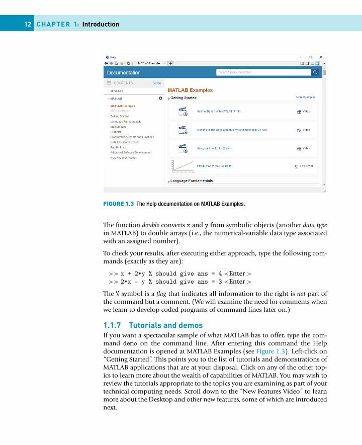
FIGURE 1.3 The Help documentation on MATLAB Examples.
The function double converts x and y from symbolic objects (another data typein MATLAB) to double arrays (i.e., the numerical-variable data type associatedwith an assigned number).
To check your results, after executing either approach, type the following com-mands (exactly as they are):
>> x + 2*y % should give ans = 4 <Enter >
>> 2*x - y % should give ans = 3 <Enter >
The % symbol is a flag that indicates all information to the right is not part ofthe command but a comment. (We will examine the need for comments whenwe learn to develop coded programs of command lines later on.)
1.1.7 Tutorials and demosIf you want a spectacular sample of what MATLAB has to offer, type the com-mand demo on the command line. After entering this command the Helpdocumentation is opened at MATLAB Examples (see Figure 1.3). Left-click on“Getting Started”. This points you to the list of tutorials and demonstrations ofMATLAB applications that are at your disposal. Click on any of the other top-ics to learn more about the wealth of capabilities of MATLAB. You may wish toreview the tutorials appropriate to the topics you are examining as part of yourtechnical computing needs. Scroll down to the “New Features Video” to learnmore about the Desktop and other new features, some of which are introducednext.
1.2 The desktop 13
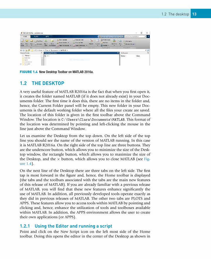
FIGURE 1.4 New Desktop Toolbar on MATLAB 2016a.
1.2 THE DESKTOP
A very useful feature of MATLAB R2016a is the fact that when you first open it,it creates the folder named MATLAB (if it does not already exist) in your Doc-uments folder. The first time it does this, there are no items in the folder and,hence, the Current Folder panel will be empty. This new folder in your Doc-uments is the default working folder where all the files your create are saved.The location of this folder is given in the first toolbar above the CommandWindow. The location is C:\Users\Clara\Documents\MATLAB. This format ofthe location was determined by pointing and left-clicking the mouse in theline just above the Command Window.
Let us examine the Desktop from the top down. On the left side of the topline you should see the name of the version of MATLAB running. In this caseit is MATLAB R2016a. On the right side of the top line are three buttons. Theyare the underscore button, which allows you to minimize the size of the Desk-top window, the rectangle button, which allows you to maximize the size ofthe Desktop, and the × button, which allows you to close MATLAB (see Fig-ure 1.4).
On the next line of the Desktop there are three tabs on the left side. The firsttap is most forward in the figure and, hence, the Home toolbar is displayed(the tabs and the toolbars associated with the tabs are the main new featuresof this release of MATLAB). If you are already familiar with a previous releaseof MATLAB, you will find that these new features enhance significantly theuse of MATLAB. In addition, all previously developed tools operate exactly asthey did in previous releases of MATLAB. The other two tabs are PLOTS andAPPS. These features allow you to access tools within MATLAB by pointing andclicking and, hence, enhance the utilization of tools and toolboxes availablewithin MATLAB. In addition, the APPS environment allows the user to createtheir own applications (or APPS).
1.2.1 Using the Editor and running a scriptPoint and click on the New Script icon on the left most side of the Hometoolbar. Doing this opens the editor in the center of the Desktop as shown in
14 CHAPTER 1: Introduction
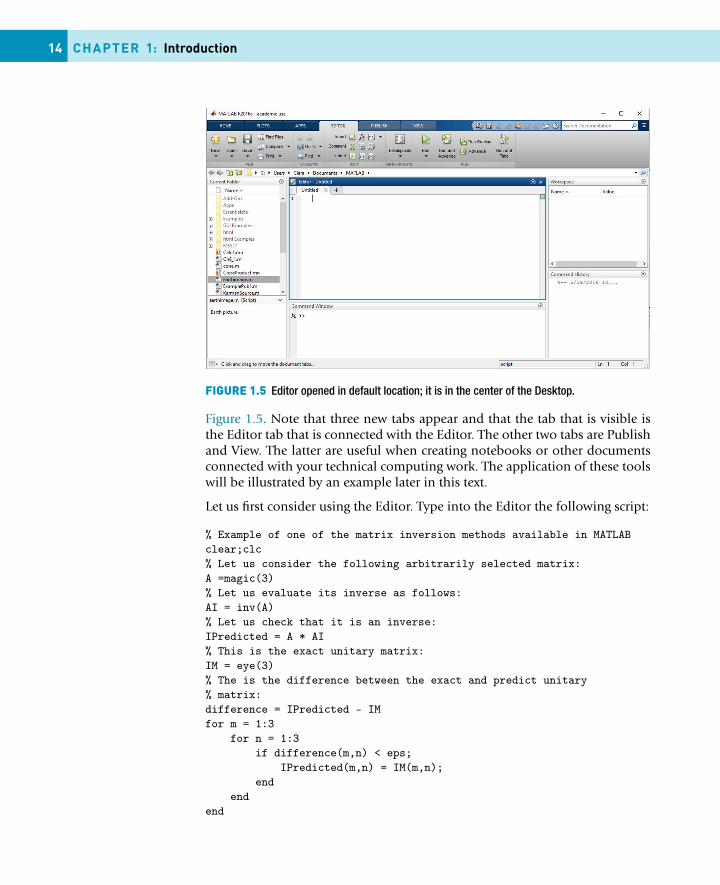
FIGURE 1.5 Editor opened in default location; it is in the center of the Desktop.
Figure 1.5. Note that three new tabs appear and that the tab that is visible isthe Editor tab that is connected with the Editor. The other two tabs are Publishand View. The latter are useful when creating notebooks or other documentsconnected with your technical computing work. The application of these toolswill be illustrated by an example later in this text.
Let us first consider using the Editor. Type into the Editor the following script:
% Example of one of the matrix inversion methods available in MATLABclear;clc% Let us consider the following arbitrarily selected matrix:A =magic(3)% Let us evaluate its inverse as follows:AI = inv(A)% Let us check that it is an inverse:IPredicted = A * AI% This is the exact unitary matrix:IM = eye(3)% The is the difference between the exact and predict unitary% matrix:difference = IPredicted - IMfor m = 1:3
for n = 1:3if difference(m,n) < eps;
IPredicted(m,n) = IM(m,n);end
endend
1.2 The desktop 15
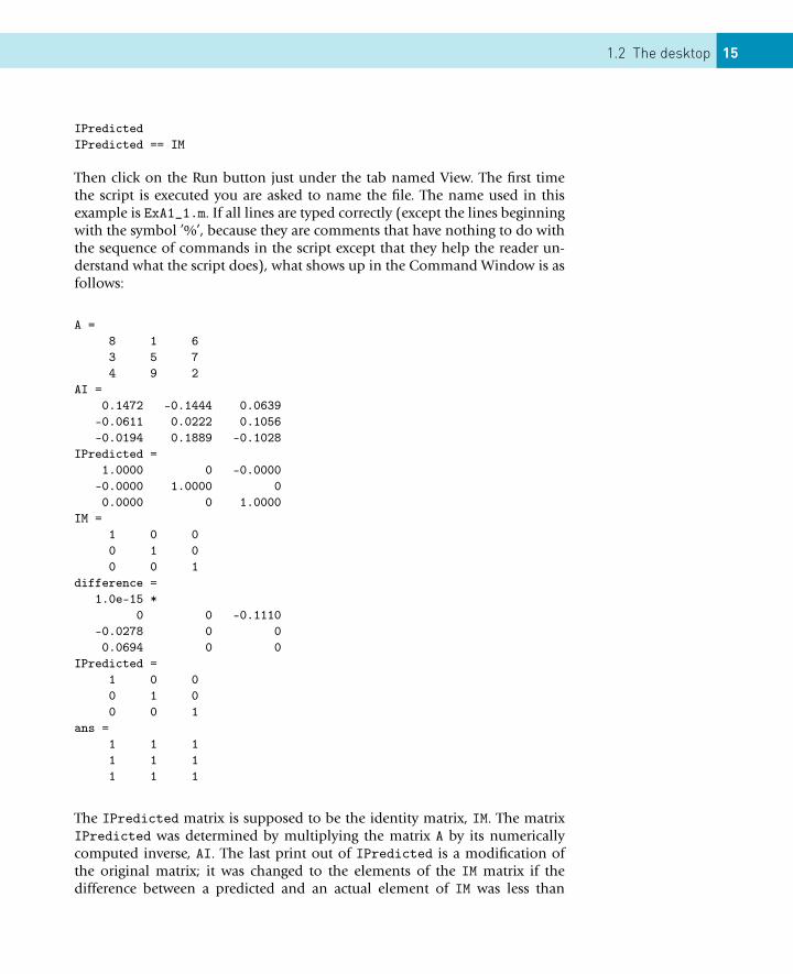
IPredictedIPredicted == IM
Then click on the Run button just under the tab named View. The first timethe script is executed you are asked to name the file. The name used in thisexample is ExA1_1.m. If all lines are typed correctly (except the lines beginningwith the symbol ’%’, because they are comments that have nothing to do withthe sequence of commands in the script except that they help the reader un-derstand what the script does), what shows up in the Command Window is asfollows:
A =8 1 63 5 74 9 2
AI =0.1472 -0.1444 0.0639
-0.0611 0.0222 0.1056-0.0194 0.1889 -0.1028
IPredicted =1.0000 0 -0.0000
-0.0000 1.0000 00.0000 0 1.0000
IM =1 0 00 1 00 0 1
difference =1.0e-15 *
0 0 -0.1110-0.0278 0 00.0694 0 0
IPredicted =1 0 00 1 00 0 1
ans =1 1 11 1 11 1 1
The IPredicted matrix is supposed to be the identity matrix, IM. The matrixIPredicted was determined by multiplying the matrix A by its numericallycomputed inverse, AI. The last print out of IPredicted is a modification ofthe original matrix; it was changed to the elements of the IM matrix if thedifference between a predicted and an actual element of IM was less than
16 CHAPTER 1: Introduction
FIGURE 1.6 Sample script created and executed in the first example of this section.
eps = 2.2204e − 16. Since the result is identical to the identity matrix, thisshows that the inverse was computed correctly (at least to within the compu-tational error of the computing environment, i.e., 0 < eps). This conclusion isa result of the fact that the ans in the above example produced the logical re-sult of 1 (or true) for all entries in the adjusted IPredicted matrix as logicallycompared with the corresponding entries in IM.
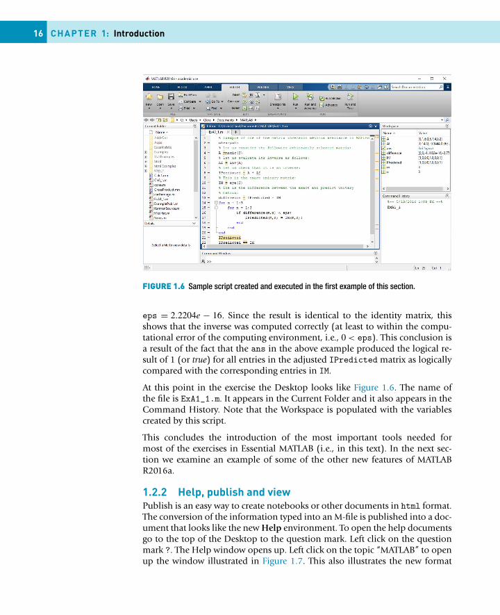
At this point in the exercise the Desktop looks like Figure 1.6. The name ofthe file is ExA1_1.m. It appears in the Current Folder and it also appears in theCommand History. Note that the Workspace is populated with the variablescreated by this script.
This concludes the introduction of the most important tools needed formost of the exercises in Essential MATLAB (i.e., in this text). In the next sec-tion we examine an example of some of the other new features of MATLABR2016a.
1.2.2 Help, publish and viewPublish is an easy way to create notebooks or other documents in html format.The conversion of the information typed into an M-file is published into a doc-ument that looks like the new Help environment. To open the help documentsgo to the top of the Desktop to the question mark. Left click on the questionmark ?. The Help window opens up. Left click on the topic “MATLAB” to openup the window illustrated in Figure 1.7. This also illustrates the new format
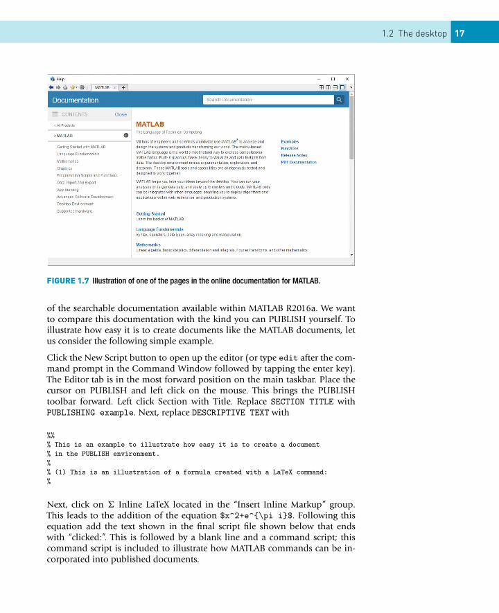
1.2 The desktop 17
FIGURE 1.7 Illustration of one of the pages in the online documentation for MATLAB.
of the searchable documentation available within MATLAB R2016a. We wantto compare this documentation with the kind you can PUBLISH yourself. Toillustrate how easy it is to create documents like the MATLAB documents, letus consider the following simple example.
Click the New Script button to open up the editor (or type edit after the com-mand prompt in the Command Window followed by tapping the enter key).The Editor tab is in the most forward position on the main taskbar. Place thecursor on PUBLISH and left click on the mouse. This brings the PUBLISHtoolbar forward. Left click Section with Title. Replace SECTION TITLE withPUBLISHING example. Next, replace DESCRIPTIVE TEXT with
%%% This is an example to illustrate how easy it is to create a document% in the PUBLISH environment.%% (1) This is an illustration of a formula created with a LaTeX command:%
Next, click on � Inline LaTeX located in the “Insert Inline Markup” group.This leads to the addition of the equation $x^2+e^{\pi i}$. Following thisequation add the text shown in the final script file shown below that endswith “clicked:”. This is followed by a blank line and a command script; thiscommand script is included to illustrate how MATLAB commands can be in-corporated into published documents.
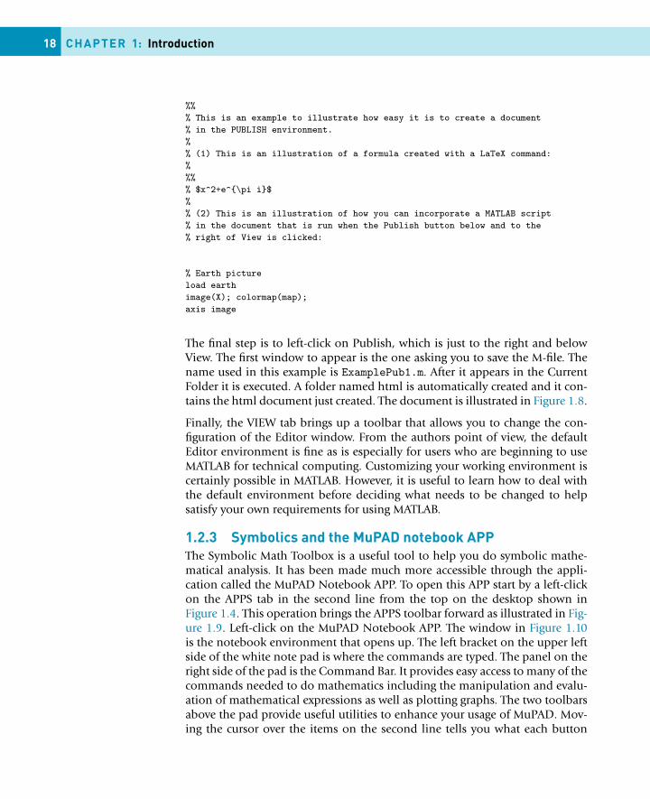
18 CHAPTER 1: Introduction
%%% This is an example to illustrate how easy it is to create a document% in the PUBLISH environment.%% (1) This is an illustration of a formula created with a LaTeX command:%%%% $x^2+e^{\pi i}$%% (2) This is an illustration of how you can incorporate a MATLAB script% in the document that is run when the Publish button below and to the% right of View is clicked:
% Earth pictureload earthimage(X); colormap(map);axis image
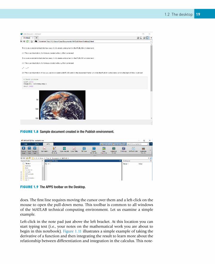
The final step is to left-click on Publish, which is just to the right and belowView. The first window to appear is the one asking you to save the M-file. Thename used in this example is ExamplePub1.m. After it appears in the CurrentFolder it is executed. A folder named html is automatically created and it con-tains the html document just created. The document is illustrated in Figure 1.8.
Finally, the VIEW tab brings up a toolbar that allows you to change the con-figuration of the Editor window. From the authors point of view, the defaultEditor environment is fine as is especially for users who are beginning to useMATLAB for technical computing. Customizing your working environment iscertainly possible in MATLAB. However, it is useful to learn how to deal withthe default environment before deciding what needs to be changed to helpsatisfy your own requirements for using MATLAB.
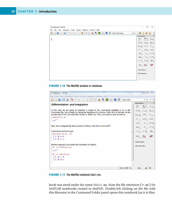
1.2.3 Symbolics and the MuPAD notebook APPThe Symbolic Math Toolbox is a useful tool to help you do symbolic mathe-matical analysis. It has been made much more accessible through the appli-cation called the MuPAD Notebook APP. To open this APP start by a left-clickon the APPS tab in the second line from the top on the desktop shown inFigure 1.4. This operation brings the APPS toolbar forward as illustrated in Fig-ure 1.9. Left-click on the MuPAD Notebook APP. The window in Figure 1.10is the notebook environment that opens up. The left bracket on the upper leftside of the white note pad is where the commands are typed. The panel on theright side of the pad is the Command Bar. It provides easy access to many of thecommands needed to do mathematics including the manipulation and evalu-ation of mathematical expressions as well as plotting graphs. The two toolbarsabove the pad provide useful utilities to enhance your usage of MuPAD. Mov-ing the cursor over the items on the second line tells you what each button
1.2 The desktop 19
FIGURE 1.8 Sample document created in the Publish environment.
FIGURE 1.9 The APPS toolbar on the Desktop.
does. The first line requires moving the cursor over them and a left-click on themouse to open the pull-down menu. This toolbar is common to all windowsof the MATLAB technical computing environment. Let us examine a simpleexample.
Left-click in the note pad just above the left bracket. At this location you canstart typing text (i.e., your notes on the mathematical work you are about tobegin in this notebook). Figure 1.11 illustrates a simple example of taking thederivative of a function and then integrating the result to learn more about therelationship between differentiation and integration in the calculus. This note-
20 CHAPTER 1: Introduction
FIGURE 1.10 The MuPAD window or notebook.
FIGURE 1.11 The MuPAD notebook Calc1.mn.
book was saved under the name Calc1.mn. Note the file extension (‘*.mn’) forMATLAB notebooks created in MuPAD. Double-left clicking on the file withthis filename in the Command Folder panel opens this notebook (as it is illus-
1.2 The desktop 21
trated in the figure). The details of this example are also provided in the figure.They are as follows:
Differentiation and integrationIn this note we are going to examine a few of the mathematical commandsavailable to us and listed in the Command Bar. Let us begin with taking thederivative of a function f. With the cursor placed on the upper left most sym-bol, a left-click on the mouse produces the following result: diff(#f, #x).The # sign is a place holder at which input is required. The next step is to pointto the right of the left bracket below and left-click to place the note pad cursorat this location. Then click on the command of interest in the Command Bar.Change #f to xn and #x to x. Then hit enter to execute the command. The resultis:
[diff(x^n, x)nxn−1
Next, let us integrate this result. First let us save the result under the name S1as follows:
[S1 := diff(x^n, x)nxn−1
Now, let us integrate. Left-click on this operation in the Command Bar to get:int(#f, #x). Replace #f with S1 and #x with x. Thus,
[S2 := int(S1,x){0 if n = 0xn if n �= 0
Hence, integration is, as expected, the inverse of differentiation. The only issue,if any, that you must keep in mind is that the constants of integration are setto zero. If you need to explicitly carry them along in your analysis, then youmust add a constant to the results at this step.
REMARK: Help is available through the help documentation. The help can beaccessed by a left click on the blue circle with the question mark in the toolbarjust above this pad.
A second example is the graphics capabilities in MuPAD. There are other plot-ting utilities within MATLAB that allow you to examine functions graphicallyand quickly. The MuPAD environment is particularly well suited for this kindof investigation. Suppose you are reading a technical article and you comeacross two interesting functions and you want to have an idea as to what theylook like. Let us examine two examples. One is the sech2(x) function whichplays an important role in nonlinear wave theory. The second is the complete
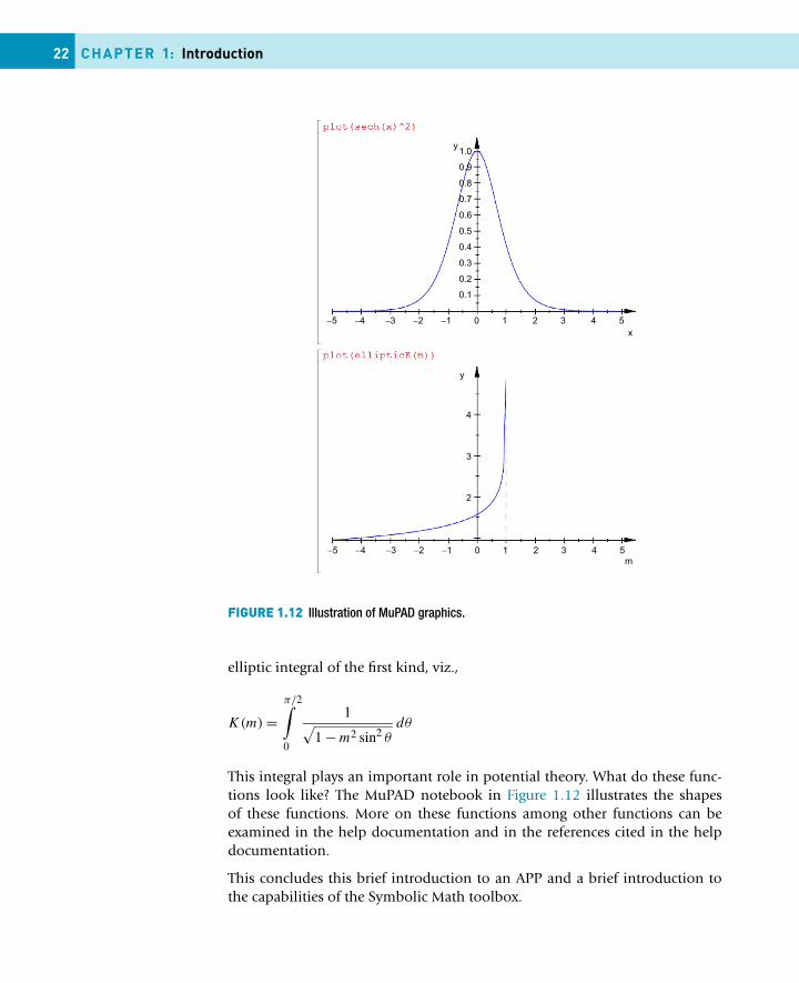
22 CHAPTER 1: Introduction
FIGURE 1.12 Illustration of MuPAD graphics.
elliptic integral of the first kind, viz.,
K(m) =π/2∫0
1√1 − m2 sin2 θ
dθ
This integral plays an important role in potential theory. What do these func-tions look like? The MuPAD notebook in Figure 1.12 illustrates the shapesof these functions. More on these functions among other functions can beexamined in the help documentation and in the references cited in the helpdocumentation.
This concludes this brief introduction to an APP and a brief introduction tothe capabilities of the Symbolic Math toolbox.
1.2 The desktop 23
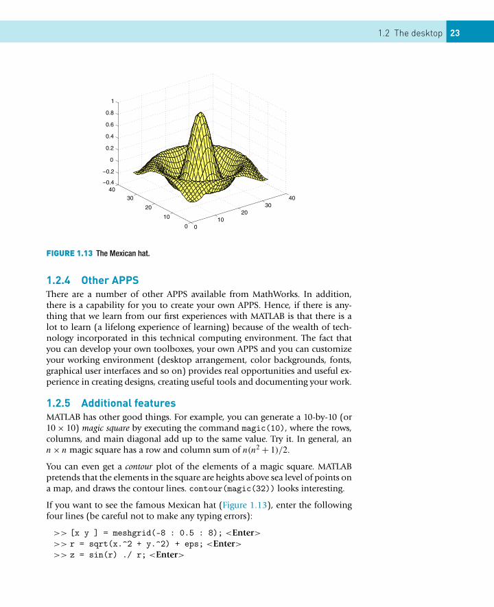
FIGURE 1.13 The Mexican hat.
1.2.4 Other APPSThere are a number of other APPS available from MathWorks. In addition,there is a capability for you to create your own APPS. Hence, if there is any-thing that we learn from our first experiences with MATLAB is that there is alot to learn (a lifelong experience of learning) because of the wealth of tech-nology incorporated in this technical computing environment. The fact thatyou can develop your own toolboxes, your own APPS and you can customizeyour working environment (desktop arrangement, color backgrounds, fonts,graphical user interfaces and so on) provides real opportunities and useful ex-perience in creating designs, creating useful tools and documenting your work.
1.2.5 Additional featuresMATLAB has other good things. For example, you can generate a 10-by-10 (or10 × 10) magic square by executing the command magic(10), where the rows,columns, and main diagonal add up to the same value. Try it. In general, ann × n magic square has a row and column sum of n(n2 + 1)/2.
You can even get a contour plot of the elements of a magic square. MATLABpretends that the elements in the square are heights above sea level of points ona map, and draws the contour lines. contour(magic(32)) looks interesting.
If you want to see the famous Mexican hat (Figure 1.13), enter the followingfour lines (be careful not to make any typing errors):
>> [x y ] = meshgrid(-8 : 0.5 : 8); <Enter>>> r = sqrt(x.^2 + y.^2) + eps; <Enter>>> z = sin(r) ./ r; <Enter>
24 CHAPTER 1: Introduction
>> mesh(z); <Enter>
surf(z) generates a faceted (tiled) view of the surface. surfc(z) or meshc(z)draws a 2D contour plot under the surface. The command
>> surf(z), shading flat <Enter>
produces a nice picture by removing the grid lines.
The following animation is an extension of the Mexican hat graphic in Fig-ure 1.13. It uses a for loop that repeats the calculation from n =−3 to n = 3in increments of 0.05. It begins with a for n =−3:0.05:3 command andends with an end command and is one of the most important constructs inprogramming. The execution of the commands between the for and end state-ments repeat 121 times in this example. The pause(0.05) puts a time delayof 0.05 seconds in the for loop to slow the animation down, so the picturechanges every 0.05 seconds until the end of the computation.
>> [x y]=meshgrid(-8:0.5:8); <Enter>>> r=sqrt( x.^2+y.^2)+eps; <Enter>>> for n=-3:0.05:3; <Enter>>> z=sin(r.*n)./r; <Enter>>> surf(z), view(-37, 38), axis([0,40,0,40,-4,4]); <Enter>>> pause(0.05) <Enter>>> end <Enter>
You can examine sound with MATLAB in any number of ways. One way is tolisten to the signal. If your PC has a speaker, try
>> load handel <Enter>>> sound(y,Fs) <Enter>
for a snatch of Handel’s Hallelujah Chorus. For different sounds try loadingchirp, gong, laughter, splat, and train. You have to run sound(y,Fs) foreach one.
If you want to see a view of the Earth from space, try
>> load earth <Enter>>> image(X); colormap(map) <Enter>>> axis image <Enter>
To enter the matrix presented at the beginning of this chapter into MATLAB,use the following command:
>> A = [1 3 5; 2 4 6] <Enter>
On the next line after the command prompt, type A(2,3) to pluck the numberfrom the second row, third column.
1.3 Sample program 25
There are a few humorous functions in MATLAB. Try why (why not?) Thentry why(2) twice. To see the MATLAB code that does this, type the followingcommand:
>> edit why <Enter>
Once you have looked at this file, close it via the pull-down menu by clickingFile at the top of the Editor desktop window and then Close Editor; do notsave the file, in case you accidently typed something and modified it.
The edit command will be used soon to illustrate the creation of an M-file likewhy.m (the name of the file executed by the command why). You will create anM-file after we go over some of the basic features of the MATLAB desktop. Moredetails on creating programs in the MATLAB environment will be explained inChapter 2.
1.3 SAMPLE PROGRAM
In Section 1.1 we saw some simple examples of how to use MATLAB by en-tering single commands or statements at the MATLAB prompt. However, youmight want to solve problems which MATLAB can’t do in one line, like find-ing the roots of a quadratic equation (and taking all the special cases intoaccount). A collection of statements to solve such a problem is called a program.In this section we look at the mechanics of writing and running two short pro-grams, without bothering too much about how they work—explanations willfollow in the next chapter.
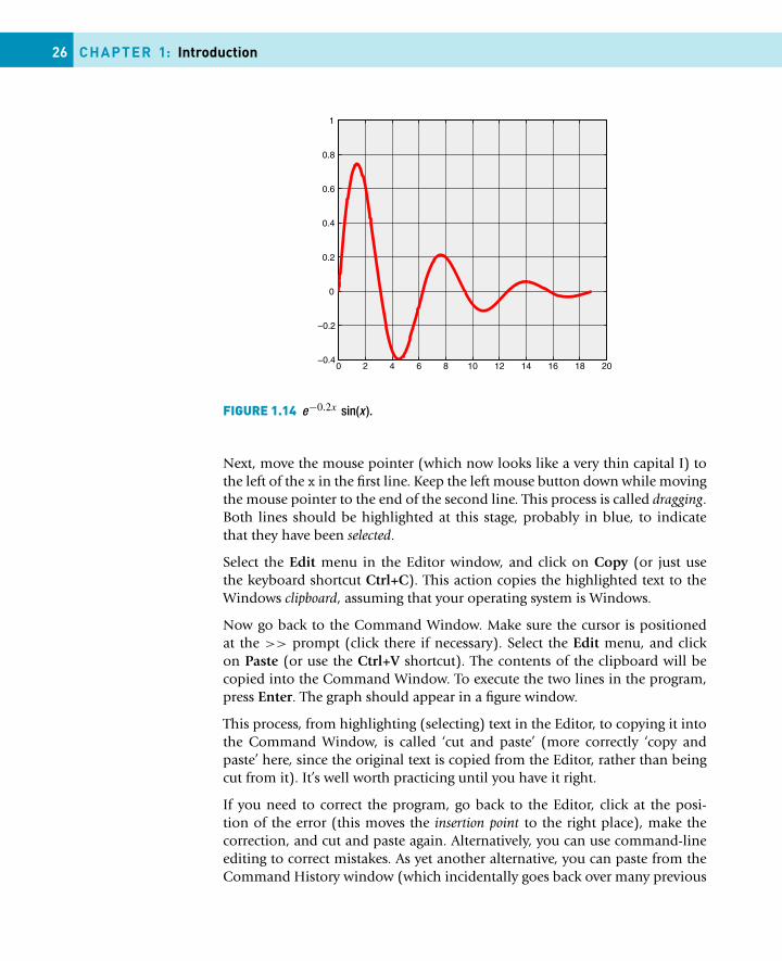
1.3.1 Cut and pasteSuppose you want to draw the graph of e−0.2x sin(x) over the domain 0 to 6π ,as shown in Figure 1.14. The Windows environment lends itself to nifty cut andpaste editing, which you would do well to master. Proceed as follows.
From the MATLAB desktop select File -> New -> Script, or click the new filebutton on the desktop toolbar (you could also type edit in the CommandWindow followed by Enter). This action opens an Untitled window in the Edi-tor/Debugger. You can regard this for the time being as a ‘scratch pad’ in whichto write programs. Now type the following two lines in the Editor, exactly asthey appear here:
x = 0 : pi/20 : 6 * pi;plot(x, exp(-0.2*x) .* sin(x), ’k’),grid
Incidentally, that is a dot (full stop, period) in front of the second * in thesecond line—a more detailed explanation later! The additional argument ’k’for plot will draw a black graph, just to be different. Change ’k’ to ’r’ togenerate a red graph if you prefer.
26 CHAPTER 1: Introduction
FIGURE 1.14 e−0.2x sin(x ).
Next, move the mouse pointer (which now looks like a very thin capital I) tothe left of the x in the first line. Keep the left mouse button down while movingthe mouse pointer to the end of the second line. This process is called dragging.Both lines should be highlighted at this stage, probably in blue, to indicatethat they have been selected.
Select the Edit menu in the Editor window, and click on Copy (or just usethe keyboard shortcut Ctrl+C). This action copies the highlighted text to theWindows clipboard, assuming that your operating system is Windows.
Now go back to the Command Window. Make sure the cursor is positionedat the >> prompt (click there if necessary). Select the Edit menu, and clickon Paste (or use the Ctrl+V shortcut). The contents of the clipboard will becopied into the Command Window. To execute the two lines in the program,press Enter. The graph should appear in a figure window.
This process, from highlighting (selecting) text in the Editor, to copying it intothe Command Window, is called ‘cut and paste’ (more correctly ‘copy andpaste’ here, since the original text is copied from the Editor, rather than beingcut from it). It’s well worth practicing until you have it right.
If you need to correct the program, go back to the Editor, click at the posi-tion of the error (this moves the insertion point to the right place), make thecorrection, and cut and paste again. Alternatively, you can use command-lineediting to correct mistakes. As yet another alternative, you can paste from theCommand History window (which incidentally goes back over many previous
1.3 Sample program 27
sessions). To select multiple lines in the Command History window keep Ctrldown while you click.
If you prefer, you can enter multiple lines directly in the Command Window.To prevent the whole group from running until you have entered the last lineuse Shift+Enter after each line until the last. Then press Enter to run all thelines.
As another example, suppose you have $1000 saved in the bank. Interest iscompounded at the rate of 9% per year. What will your bank balance be af-ter one year? Now, if you want to write a MATLAB program to find your newbalance, you must be able to do the problem yourself in principle. Even witha relatively simple problem like this, it often helps first to write down a roughstructure plan:
1. Get the data (initial balance and interest rate) into MATLAB.2. Calculate the interest (9% of $1000, i.e., $90).3. Add the interest to the balance ($90 + $1000, i.e., $1090).4. Display the new balance.
Go back to the Editor. To clear out any previous text, select it as usual by drag-ging (or use Ctrl+A), and press the Del key. By the way, to de-select highlightedtext, click anywhere outside the selection area. Enter the following program,and then cut and paste it to the Command Window.
balance = 1000;rate = 0.09;interest = rate * balance;balance = balance + interest;disp( ’New balance:’ );disp( balance );
When you press Enter to run it, you should get the following output in theCommand Window:
New balance:1090
1.3.2 Saving a program: script filesWe have seen how to cut and paste between the Editor and the CommandWindow in order to write and run MATLAB programs. Obviously you need tosave the program if you want to use it again later.
To save the contents of the Editor, select File -> Save from the Editor menubar.A Save file as: dialogue box appears. Select a folder and enter a file name,which must have the extension .m, in the File name: box, e.g., junk.m. Click
28 CHAPTER 1: Introduction
on Save. The Editor window now has the title junk.m. If you make subsequentchanges to junk.m in the Editor, an asterisk appears next to its name at the topof the Editor until you save the changes.
A MATLAB program saved from the Editor (or any ASCII text editor) with theextension .m is called a script file, or simply a script. (MATLAB function filesalso have the extension .m. We therefore refer to both script and function filesgenerally as M-files.) The special significance of a script file is that, if you enterits name at the command-line prompt, MATLAB carries out each statement inthe script file as if it were entered at the prompt.
The rules for script file names are the same as those for MATLAB variable names(see the next Chapter 2, Section 2.1).
As an example, save the compound interest program above in a script file underthe name compint.m. Then simply enter the name
compint
at the prompt in the Command Window (as soon as you hit Enter). The state-ments in compint.m will be carried out exactly as if you had pasted theminto the Command Window. You have effectively created a new MATLAB com-mand, viz., compint.
A script file may be listed in the Command Window with the command type,e.g.,
type compint
(the extension .m may be omitted).
Script files provide a useful way of managing large programs which you donot necessarily want to paste into the Command Window every time you runthem.
Current directoryWhen you run a script, you have to make sure that MATLAB’s current folder(indicated in the toolbar just above the Current Folder) is set to the folder (ordirectory) in which the script is saved. To change the current folder type thepath for the new current folder in the toolbar, or select a folder from the drop-down list of previous working folders, or click on the browse button (it is thefirst folder with the green arrow that is to the left of the field that indicates thelocation of the Current Folder. Select a new location for saving and executingfiles (e.g., if you create files for different courses, you may wish to save yourwork in folders with the names or numbers of the courses that you are taking).
1.3 Sample program 29
You can change the current folder from the command line with cd command,e.g.,
cd \mystuff
The command cd by itself returns the name of the current directory or currentfolder (as it is now called in the latest versions of MATLAB).
Running a script from the current folder browserA handy way to run a script is as follows. Select the file in the Current Directorybrowser. Right-click it. The context menu appears (context menus are a generalfeature of the desktop). Select Run from the context menu. The results appearin the Command Window. If you want to edit the script, select Open from thecontext menu.
1.3.3 A program in actionWe will now discuss in detail how the compound interest program works.
The MATLAB system is technically called an interpreter (as opposed to a com-piler). This means that each statement presented to the command line is trans-lated (interpreted) into language the computer understands better, and thenimmediately carried out.
A fundamental concept in MATLAB is how numbers are stored in the com-puter’s random access memory (RAM). If a MATLAB statement needs to store anumber, space in the RAM is set aside for it. You can think of this part of thememory as a bank of boxes or memory locations, each of which can hold onlyone number at a time. These memory locations are referred to by symbolicnames in MATLAB statements. So the statement
balance = 1000
allocates the number 1000 to the memory location named balance. Since thecontents of balance may be changed during a session it is called a variable.
The statements in our program are therefore interpreted by MATLAB as follows:
1. Put the number 1000 into variable balance.2. Put the number 0.09 into variable rate.3. Multiply the contents of rate by the contents of balance and put the an-
swer in interest.4. Add the contents of balance to the contents of interest and put the an-
swer in balance.5. Display (in the Command Window) the message given in single quotes.
30 CHAPTER 1: Introduction
6. Display the contents of balance.
It hardly seems necessary to stress this, but these interpreted statements arecarried out in order from the top down. When the program has finished running,the variables used will have the following values:
balance : 1090interest : 90rate : 0.09
Note that the original value of balance (1000) is lost.
Try the following exercises:
1. Run the program as it stands.2. Change the first statement in the program to read
balance = 2000;
Make sure that you understand what happens now when the program runs.3. Leave out the line
balance = balance + interest;
and re-run. Can you explain what happens?4. Try to rewrite the program so that the original value of balance is not lost.
A number of questions have probably occurred to you by now, such as
� What names may be used for variables?� How can numbers be represented?� What happens if a statement won’t fit on one line?� How can we organize the output more neatly?
These questions will be answered in the next chapter. However, before we writeany more complete programs there are some additional basic concepts whichneed to be introduced. These concepts are introduced in the next chapter.
SUMMARY� MATLAB is a matrix-based computer system designed to assist in scientific
and engineering problem solving.� To use MATLAB, you enter commands and statements on the command
line in the Command Window. They are carried out immediately.� quit or exit terminates MATLAB.� clc clears the Command Window.� help and lookfor provide help.
1.3 Exercises 31
� plot draws an x-y graph in a figure window.� grid draws grid lines on a graph.
EXERCISES1.1 Give values to variables a and b on the command line, e.g., a = 3 and
b = 5. Write some statements to find the sum, difference, product andquotient of a and b.
1.2 In Section 1.2.5 of the text a script is given for an animation of the Mexicanhat problem. Type this into the editor, save it and execute it. Once youfinish debugging it and it executes successfully try modifying it. (a) Changethe maximum value of n from 3 to 4 and execute the script. (b) Changethe time delay in the pause function from 0.05 to 0.1. (c) Change thez=sin(r.*n)./r; command line to z=cos(r.*n); and execute the script.
1.3 Assign a value to the variable x on the command line, e.g., x = 4 * pi^2.What is the square root of x? What is the cosine of the square root of x?
1.4 Assign a value to the variable y on the command line as follows: y = -1.What is the square root of y? Show that the answer is
ans =0 + 1.0000i
Yes, MATLAB deals with complex numbers (not just real numbers). Hencethe symbol i should not be used as an index or as a variable name. Bydefault, it is equal to the square root of −1. (Also, when necessary, j isused in MATLAB as a symbol for
√−1. Hence, it also should not be usedas an index or as a variable name.) Give an example of how you have usedcomplex numbers in your studies of mathematics and the sciences up tothis point in your education.
Solutions to many of the exercises are in Appendix D.
APPENDIX 1.A SUPPLEMENTARY MATERIAL
Supplementary material related to this chapter can be found online at http://dx.doi.org/10.1016/B978-0-08-100877-5.00002-5.
CONTENTS
Variables ............... 33Case sensitivity........ 34
The workspace .... 34Adding commonly usedconstants to theworkspace ............... 35
Arrays: Vectors andmatrices................ 36Initializing vectors:Explicit lists ............. 36Initializing vectors: Thecolon operator ......... 37The linspace andlogspace functions .. 38Transposing vectors 39Subscripts ............... 39Matrices .................. 40Capturing output ..... 40Structure plan ......... 41
Vertical motionunder gravity ....... 42
Operators,expressions, andstatements ........... 44Numbers ................. 45Data types................ 45Arithmetic operators46
CHAPTER 2
MATLAB Fundamentals
THE OBJECTIVE OF THIS CHAPTER IS TO INTRODUCE SOMEOF THE FUNDAMENTALS OF MATLAB PROGRAMMING,INCLUDING:
� Variables, operators, and expressions� Arrays (including vectors and matrices)� Basic input and output� Repetition (for)� Decisions (if)
The tools introduced in this chapter are sufficient to begin solving numerousscientific and engineering problems you may encounter in your course workand in your profession. The last part of this chapter and the next chapterdescribe an approach to designing reasonably good programs to initiate thebuilding of tools for your own toolbox.
2.1 VARIABLESVariables are fundamental to programming. In a sense, the art of programmingis this:
Getting the right values in the right variables at the right time
A variable name (like the variable balance that we used in Chapter 1) mustcomply with the following two rules:
� It may consist only of the letters a–z, the digits 0–9, and the underscore ( _ ).� It must start with a letter.
The name may be as long as you like, but MATLAB only remembers the first 63characters (to check this on your version, execute the command namelength-max in the Command Window of the MATLAB desktop). Examples of valid
33Essential MATLAB for Engineers and Scientists. DOI:10.1016/B978-0-08-100877-5.00003-7Copyright © 2017 Daniel T. Valentine. Published by Elsevier Ltd. All rights reserved.
Operatorprecedence .............. 46The colon operator .. 47The transposeoperator................... 47Arithmetic operationson arrays ................. 48Expressions ............. 49Statements .............. 49Statements,commands, andfunctions.................. 50Formulavectorization .............51
Output.................... 54The disp statement . 54The formatcommand ................ 55Scale factors............ 56
Repeating withfor.......................... 57Square roots withNewton’s method .... 58Factorials! ............... 59Limit of a sequence . 59The basic forconstruct ................. 60for in a single line ... 61More general for..... 61Avoid for loops byvectorizing! .............. 62
Decisions .............. 64The one-line ifstatement ................ 64The if-elseconstruct ................. 66The one-line if-elsestatement ................ 67elseif...................... 67Logical operators .... 68Multiple ifs versuselseif...................... 69Nested ifs............... 70Vectorizing ifs?........71The switchstatement .................71
34 CHAPTER 2: MATLAB Fundamentals
variable names are r2d2 and pay_day. Examples of invalid names (why?) arepay-day, 2a, name$, and _2a.
A variable is created simply by assigning a value to it at the command line orin a program—for example,
a = 98
If you attempt to refer to a nonexistent variable you will get the error message
??? Undefined function or variable ...
The official MATLAB documentation refers to all variables as arrays, whetherthey are single-valued (scalars) or multi-valued (vectors or matrices). In otherwords, a scalar is a 1-by-1 array—an array with a single row and a single columnwhich, of course, is an array of one item.
2.1.1 Case sensitivityMATLAB is case-sensitive, which means it distinguishes between upper- andlowercase letters. Thus, balance, BALANCE and BaLance are three different vari-ables. Many programmers write variable names in lowercase except for the firstletter of the second and subsequent words, if the name consists of more thanone word run together. This style is known as camel caps, the uppercase let-ters looking like a camel’s humps (with a bit of imagination). Examples arecamelCaps, milleniumBug, dayOfTheWeek. Some programmers prefer to sep-arate words with underscores.
Command and function names are also case-sensitive. However, note thatwhen you use the command-line help, function names are given in capitals(e.g., CLC) solely to emphasize them. You must not use capitals when runningbuilt-in functions and commands!
2.2 THE WORKSPACE
Another fundamental concept in MATLAB is the workspace. Enter the commandclear and then rerun the compound interest program (see Section 1.3.2). Nowenter the command who. You should see a list of variables as follows:
Your variables are:
balance interest rate
All the variables you create during a session remain in the workspace until youclear them. You can use or change their values at any stage during the session.
Complexnumbers ............... 72
Summary .............. 74
Exercises .............. 76
Supplementarymaterial ................ 81
2.2 The workspace 35
The command who lists the names of all the variables in your workspace. Thefunction ans returns the value of the last expression evaluated but not assignedto a variable. The command whos lists the size of each variable as well:
Name Size Bytes Class
balance 1x1 8 double arrayinterest 1x1 8 double arrayrate 1x1 8 double array
Each variable here occupies eight bytes of storage. A byte is the amount of com-puter memory required for one character (if you are interested, one byte is thesame as eight bits). These variables each have a size of “1 by 1,” because theyare scalars, as opposed to vectors or matrices (although as mentioned above,MATLAB regards them all as 1-by-1 arrays). The Class double array meansthat the variable holds numeric values as double-precision floating-point (seeSection 2.5).
The command clear removes all variables from the workspace. A particularvariable can be removed from the workspace (e.g., clear rate). More thanone variable can also be cleared (e.g., clear rate balance). Separate the vari-able names with spaces, not commas.
When you run a program, any variables created by it remain in the workspaceafter it runs. This means that existing variables with the same names are over-written.
The Workspace browser on the desktop provides a handy visual representationof the workspace. You can view and even change the values of workspace vari-ables with the Array Editor. To activate the Array Editor click on a variable in theWorkspace browser or right-click to get the more general context menu. Fromthe context menu you can draw graphs of workspace variables in various ways.
2.2.1 Adding commonly used constants to the workspaceIf you often use the same physical or mathematical constants in your MATLABsessions, you can save them in an M-file and run the file at the start of a session.For example, the following statements can be saved in myconst.m:
g = 9.81; % acceleration due to gravityavo = 6.023e23; % Avogadro’s numbere = exp(1); % base of natural logpi_4 = pi / 4;log10e = log10( e );bar_to_kP = 101.325; % atmospheres to kiloPascals
36 CHAPTER 2: MATLAB Fundamentals
If you run myconst at the start of a session, these six variables will be partof the workspace and will be available for the rest of the session or until youclear them. This approach to using MATLAB is like a notepad (it is one ofmany ways). As your experience grows, you will discover many more utilitiesand capabilities associated with MATLAB’s computational and analytical envi-ronment.
2.3 ARRAYS: VECTORS AND MATRICES
As mentioned in Chapter 1, the name MATLAB stands for Matrix Laboratorybecause MATLAB has been designed to work with matrices. A matrix is a rect-angular object (e.g., a table) consisting of rows and columns. We will postponemost of the details of proper matrices and how MATLAB works with them untilChapter 6.
A vector is a special type of matrix, having only one row or one column. Vectorsare called lists or arrays in other programming languages. If you haven’t comeacross vectors officially yet, don’t worry—just think of them as lists of numbers.
MATLAB handles vectors and matrices in the same way, but since vectorsare easier to think about than matrices, we will look at them first. This willenhance your understanding and appreciation of many aspects of MATLAB.As mentioned above, MATLAB refers to scalars, vectors, and matrices gener-ally as arrays. We will also use the term array generally, with vector and ma-trix referring to the one-dimensional (1D) and two-dimensional (2D) arrayforms.
2.3.1 Initializing vectors: Explicit listsAs a start, try the accompanying short exercises on the command line. Theseare all examples of the explicit list method of initializing vectors. (You won’tneed reminding about the command prompt � or the need to <Enter> anymore, so they will no longer appear unless the context absolutely demands it.)
Exercises2.1 Enter a statement like
x = [1 3 0 -1 5]
Can you see that you have created a vector (list) with five elements? (Make sureto leave out the semicolon so that you can see the list. Also, make sure you hitEnter to execute the command.)
2.2 Enter the command disp(x) to see how MATLAB displays a vector.
2.3 Enter the command whos (or look in the Workspace browser). Under theheading Size you will see that x is 1 by 5, which means 1 row and 5 columns.You will also see that the total number of elements is 5.
2.3 Arrays: Vectors and matrices 37
2.4 You can use commas instead of spaces between vector elements if you like. Trythis:
a = [5,6,7]
2.5 Don’t forget the commas (or spaces) between elements; otherwise, you couldend up with something quite different:
x = [130 - 15]
What do you think this gives? Take the space between the minus sign and 15 tosee how the assignment of x changes.
2.6 You can use one vector in a list for another one. Type in the following:
a = [1 2 3];b = [4 5];c = [a -b];
Can you work out what c will look like before displaying it?
2.7 And what about this?
a = [1 3 7];a = [a 0 -1];
2.8 Enter the following
x = [ ]
Note in the Workspace browser that the size of x is given as 0 by 0 because x isempty. This means x is defined and can be used where an array is appropriatewithout causing an error; however, it has no size or value.Making x empty is not the same as saying x = 0 (in the latter case x has size 1by 1) or clear x (which removes x from the workspace, making it undefined).An empty array may be used to remove elements from an array (seeSection 2.3.5).
Remember the following important rules:
� Elements in the list must be enclosed in square brackets, not parentheses.� Elements in the list must be separated either by spaces or by commas.
2.3.2 Initializing vectors: The colon operatorA vector can also be generated (initialized) with the colon operator, as we sawin Chapter 1. Enter the following statements:
x = 1:10
(elements are the integers 1, 2, . . . , 10)
x = 1:0.5:4
38 CHAPTER 2: MATLAB Fundamentals
(elements are the values 1, 1.5, . . . , 4 in increments of 0.5. Note that if thecolons separate three values, the middle value is the increment);
x = 10:-1:1
(elements are the integers 10, 9, . . . , 1, since the increment is negative);
x = 1:2:6
(elements are 1, 3, 5; note that when the increment is positive but not equal to1, the last element is not allowed to exceed the value after the second colon);
x = 0:-2:-5
(elements are 0,−2,−4; note that when the increment is negative but not equalto −1, the last element is not allowed to be less than the value after the secondcolon);
x = 1:0
(a complicated way of generating an empty vector!).
2.3.3 The linspace and logspace functionsThe function linspace can be used to initialize a vector of equally spacedvalues:
linspace(0, pi/2, 10)
creates a vector of 10 equally spaced points from 0 to π/2 (inclusive).
The function logspace can be used to generate logarithmically spaced data.It is a logarithmic equivalent of linspace. To illustrate the application oflogspace try the following:
y = logspace(0, 2, 10)
This generates the following set of numbers 10 numbers between 100 to102 (inclusive): 1.0000, 1.6681, 2.7826, 4.6416, 7.7426, 12.9155, 21.5443,35.9381, 59.9484, 100.0000. If the last number in this function call is omit-ted, the number of values of y computed is by default 50. What is the intervalbetween the numbers 1 and 100 in this example? To compute the distancebetween the points you can implement the following command:
2.3 Arrays: Vectors and matrices 39
dy = diff(y)yy = y(1:end-1) + dy./2plot(yy,dy)
You will find that you get a straight line from the point (yy, dy) =(1.3341,0.6681) to the point (79.9742,40.0516). Thus, the logspace functionproduces a set of points with an interval between them that increases linearlywith y. The variable yy was introduced for two reasons. The first was to gener-ate a vector of the same length as dy. The second was to examine the increasein the interval with increase in y that is obtained with the implementation oflogspace.
2.3.4 Transposing vectorsAll of the vectors examined so far are row vectors. Each has one row and severalcolumns. To generate the column vectors that are often needed in mathematics,you need to transpose such vectors—that is, you need to interchange their rowsand columns. This is done with the single quote, or apostrophe (’), which is thenearest MATLAB can get to the mathematical prime (′) that is often used toindicate the transpose.
Enter x = 1:5 and then enter x’ to display the transpose of x. Note that x itselfremains a row vector. Alternatively, or you can create a column vector directly:
y = [1 4 8 0 -1]’
2.3.5 SubscriptsWe can refer to particular elements of a vector by means of subscripts. Try thefollowing:
1. Enter r = rand(1,7). This gives you a row vector of seven random numbers.2. Enter r(3). This will display the third element of r. The numeral 3 is the
subscript.3. Enter r(2:4). This should give you the second, third, and fourth elements.4. What about r(1:2:7) and r([1 7 2 6])?5. Use an empty vector to remove elements from a vector:
r([1 7 2]) = [ ]
This will remove elements 1, 7, and 2.
To summarize:
� A subscript is indicated by parentheses.� A subscript may be a scalar or a vector.� In MATLAB subscripts always start at 1.� Fractional subscripts are not allowed.
40 CHAPTER 2: MATLAB Fundamentals
2.3.6 MatricesA matrix may be thought of as a table consisting of rows and columns. You cre-ate a matrix just as you do a vector, except that a semicolon is used to indicatethe end of a row. For example, the statement
a = [1 2 3; 4 5 6]
results in
a =1 2 34 5 6
A matrix may be transposed: With a initialized as above, the statement a’ re-sults in
ans =1 42 53 6
A matrix can be constructed from column vectors of the same length. Thus, thestatements
x = 0:30:180;table = [x’ sin(x*pi/180)’]
result in
table =0 0
30.0000 0.500060.0000 0.866090.0000 1.0000120.0000 0.8660150.0000 0.5000180.0000 0.0000
2.3.7 Capturing outputYou can use cut and paste techniques to tidy up the output from MATLABstatements if this is necessary for some sort of presentation. Generate the tableof angles and sines as shown above. Select all seven rows of numerical output
2.3 Arrays: Vectors and matrices 41
in the Command Window, and copy the selected output to the Editor. Youcan then edit the output, for example, by inserting text headings above eachcolumn (this is easier than trying to get headings to line up over the columnswith a disp statement). The edited output can in turn be pasted into a reportor printed as is (the File menu has a number of printing options).
Another way of capturing output is with the diary command. The command
diary filename
copies everything that subsequently appears in the Command Window to thetext file filename. You can then edit the resulting file with any text editor (in-cluding the MATLAB Editor). Stop recording the session with
diary off
Note that diary appends material to an existing file—that is, it adds new infor-mation to the end of it.
2.3.8 Structure planA structure plan is a top-down design of the steps required to solve a particularproblem with a computer. It is typically written in what is called pseudo-code—that is, statements in English, mathematics, and MATLAB describing in detailhow to solve a problem. You don’t have to be an expert in any particular com-puter language to understand pseudo-code. A structure plan may be written ata number of levels, each of increasing complexity, as the logical structure of theprogram is developed.
Suppose we want to write a script to convert a temperature on the Fahrenheitscale (where water freezes and boils at 32◦ and 212◦, respectively) to the Celsiusscale. A first-level structure plan might be a simple statement of the problem:
1. Initialize Fahrenheit temperature2. Calculate and display Celsius temperature3. Stop
Step 1 is pretty straightforward. Step 2 needs elaborating, so the second-levelplan could be something like this:
1. Initialize Fahrenheit temperature (F)2. Calculate Celsius temperature (C) as follows: Subtract 32 from F and mul-
tiply by 5/93. Display the value of C4. Stop
There are no hard and fast rules for writing structure plans. The essential pointis to cultivate the mental discipline of getting the problem logic clear before
42 CHAPTER 2: MATLAB Fundamentals
attempting to write the program. The top-down approach of structure plansmeans that the overall structure of a program is clearly thought out before youhave to worry about the details of syntax (coding). This reduces the number oferrors enormously.
A script to implement this is as follows:
% Script file to convert temperatures from F to C% Daniel T. Valentine ............ 2006/2008/2012%F = input(’ Temperature in degrees F: ’)
C = (F - 32) * 5 / 9;disp([’ Temperature in degrees C = ’,num2str(C)])% STOP
Two checks of the tool were done. They were for F = 32, which gave C = 0, andF = 212, which gave C = 100. The results were found to be correct and hencethis simple script is, as such, validated.
The essence of any structure plan and, hence, any computer program can besummarized as follows:
1. Input: Declare and assign input variables.2. Operations: Solve expressions that use the input variables.3. Output: Display in graphs or tables the desired results.
2.4 VERTICAL MOTION UNDER GRAVITY
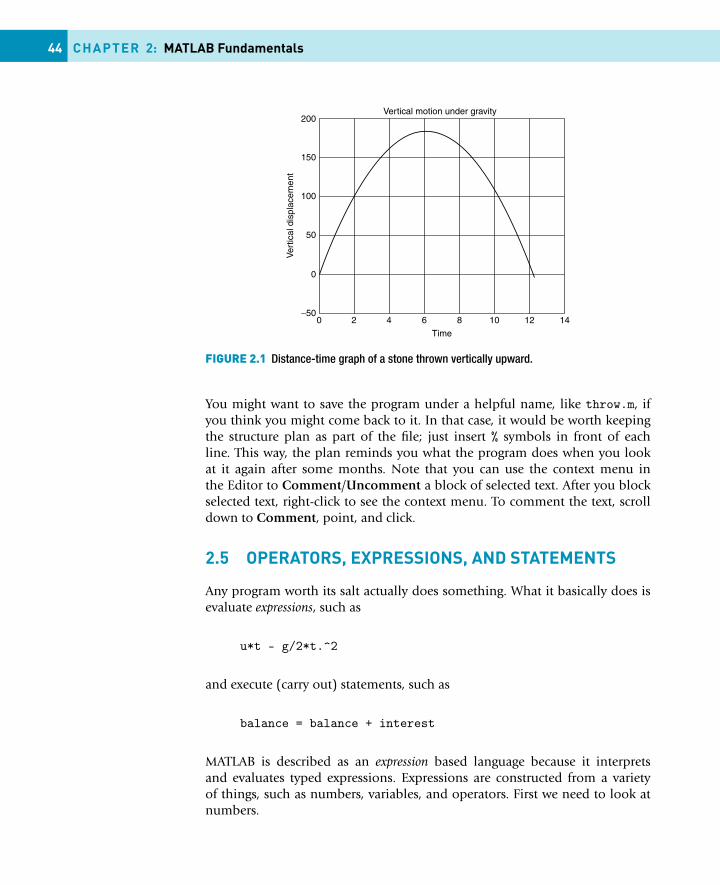
If a stone is thrown vertically upward with an initial speed u, its vertical dis-placement s after an elapsed time t is given by the formula s = ut − gt2/2,where g is the acceleration due to gravity. Air resistance is ignored. We wouldlike to compute the value of s over a period of about 12.3 seconds at intervalsof 0.1 seconds, and plot the distance–time graph over this period, as shown inFigure 2.1. The structure plan for this problem is as follows:
1. % Assign the data (g, u, and t) to MATLAB variables2. % Calculate the value of s according to the formula3. % Plot the graph of s against t4. % Stop
This plan may seem trivial and a waste of time to write down. Yet you wouldbe surprised how many beginners, preferring to rush straight to the computer,start with step 2 instead of step 1. It is well worth developing the mental disci-pline of structure-planning your program first. You can even use cut and pasteto plan as follows:
2.4 Vertical motion under gravity 43
1. Type the structure plan into the Editor (each line preceded by % as shownabove).
2. Paste a second copy of the plan directly below the first.3. Translate each line in the second copy into a MATLAB statement or state-
ments (add % comments as in the example below).4. Finally, paste all the translated MATLAB statements into the Command
Window and run them (or you can just click on the green triangle in thetoolbar of the Editor to execute your script).
5. If necessary, go back to the Editor to make corrections and repaste the cor-rected statements to the Command Window (or save the program in theEditor as an M-file and execute it).
You might like to try this as an exercise before looking at the final program,which is as follows:
% Vertical motion under gravityg = 9.81; % acceleration due% to gravityu = 60; % initial velocity in% metres/sect = 0 : 0.01 : 12.3; % time in secondss = u * t - g / 2 * t .^ 2; % vertical displacement% in metresplot(t, s,’k’,’LineWidth’,3)title( ’Vertical motion under gravity’ )xlabel( ’time’ ), ylabel( ’vertical displacement’ )grid
The graphical output is shown in Figure 2.1.
Note the following points:
� Anything in a line following the symbol % is ignored by MATLAB and maybe used as a comment (description).
� The statement t = 0 : 0.1 : 12.3 sets up a vector.� The formula for s is evaluated for every element of the vector t, making an-
other vector.� The expression t.^2 squares each element in t. This is called an array op-
eration and is different from squaring the vector itself, which is a matrixoperation, as we will see later.
� More than one statement can be entered on the same line if the statementsare separated by commas.
� A statement or group of statements can be continued to the next line withan ellipsis of three or more dots (...).
� The statement disp([t’ s’]) first transposes the row vectors t and s intotwo columns and constructs a matrix from them, which is then displayed.
44 CHAPTER 2: MATLAB Fundamentals
FIGURE 2.1 Distance-time graph of a stone thrown vertically upward.
You might want to save the program under a helpful name, like throw.m, ifyou think you might come back to it. In that case, it would be worth keepingthe structure plan as part of the file; just insert % symbols in front of eachline. This way, the plan reminds you what the program does when you lookat it again after some months. Note that you can use the context menu inthe Editor to Comment/Uncomment a block of selected text. After you blockselected text, right-click to see the context menu. To comment the text, scrolldown to Comment, point, and click.
2.5 OPERATORS, EXPRESSIONS, AND STATEMENTS
Any program worth its salt actually does something. What it basically does isevaluate expressions, such as
u*t - g/2*t.^2
and execute (carry out) statements, such as
balance = balance + interest
MATLAB is described as an expression based language because it interpretsand evaluates typed expressions. Expressions are constructed from a varietyof things, such as numbers, variables, and operators. First we need to look atnumbers.
2.5 Operators, expressions, and statements 45
2.5.1 NumbersNumbers can be represented in MATLAB in the usual decimal form (fixed point)with an optional decimal point,
1.2345 -123 .0001
They may also be represented in scientific notation. For example, 1.2345 × 10⁹
may be represented in MATLAB as 1.2345e9. This is also called floating-pointnotation. The number has two parts: the mantissa, which may have an optionaldecimal point (1.2345 in this example) and the exponent (9), which must bean integer (signed or unsigned). Mantissa and exponent must be separated bythe letter e (or E). The mantissa is multiplied by the power of 10 indicated bythe exponent.
Note that the following is not scientific notation: 1.2345*10^9. It is actu-ally an expression involving two arithmetic operations (* and ^) and thereforemore time consuming. Use scientific notation if the numbers are very smallor very large, since there’s less chance of making a mistake (e.g., represent0.000000001 as 1e-9).
On computers using standard floating-point arithmetic, numbers are repre-sented to approximately 16 significant decimal digits. The relative accuracy ofnumbers is given by the function eps, which is defined as the distance be-tween 1.0 and the next largest floating-point number. Enter eps to see its valueon your computer.
The range of numbers is roughly ±10−308 to ±10308. Precise values for yourcomputer are returned by the MATLAB functions realmin and realmax.
As an exercise, enter the following numbers at the command prompt in scien-tific notation (answers follow in parentheses):
1.234 × 10⁵, −8.765 × 10⁻⁴, 10−15, −1012
(1.234e + 05, −8.765e−04, 1e−15, −1e + 12)
2.5.2 Data typesMATLAB has more than a dozen fundamental data types (or classes). The de-fault numeric data type is double precision; all MATLAB computations are indouble precision. More information on data types can be found in the Helpindex.
MATLAB also supports signed and unsigned integer types and single-precisionfloating-point, by means of functions such as int8, uint8, single, and thelike. However, before mathematical operations can be performed on suchtypes, they must be converted to double precision using the double function.
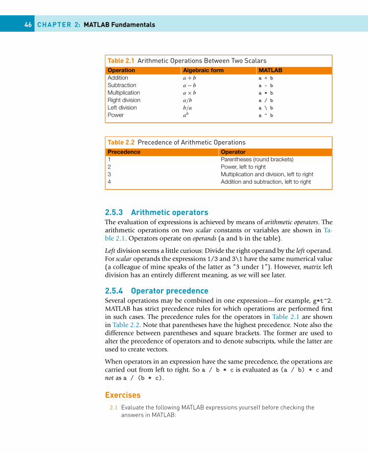
46 CHAPTER 2: MATLAB Fundamentals
Table 2.1 Arithmetic Operations Between Two ScalarsOperation Algebraic form MATLABAddition a + b a + bSubtraction a − b a - bMultiplication a × b a * bRight division a/b a / bLeft division b/a a \ bPower ab a ^ b
Table 2.2 Precedence of Arithmetic OperationsPrecedence Operator1 Parentheses (round brackets)2 Power, left to right3 Multiplication and division, left to right4 Addition and subtraction, left to right
2.5.3 Arithmetic operatorsThe evaluation of expressions is achieved by means of arithmetic operators. Thearithmetic operations on two scalar constants or variables are shown in Ta-ble 2.1. Operators operate on operands (a and b in the table).
Left division seems a little curious: Divide the right operand by the left operand.For scalar operands the expressions 1/3 and 3\1 have the same numerical value(a colleague of mine speaks of the latter as “3 under 1”). However, matrix leftdivision has an entirely different meaning, as we will see later.
2.5.4 Operator precedenceSeveral operations may be combined in one expression—for example, g*t^2.MATLAB has strict precedence rules for which operations are performed firstin such cases. The precedence rules for the operators in Table 2.1 are shownin Table 2.2. Note that parentheses have the highest precedence. Note also thedifference between parentheses and square brackets. The former are used toalter the precedence of operators and to denote subscripts, while the latter areused to create vectors.
When operators in an expression have the same precedence, the operations arecarried out from left to right. So a / b * c is evaluated as (a / b) * c andnot as a / (b * c).
Exercises2.1 Evaluate the following MATLAB expressions yourself before checking the
answers in MATLAB:
2.5 Operators, expressions, and statements 47
1 + 2 * 34 / 2 * 21 + 2 / 41 + 2 \ 42 * 2 ^ 32 * 3 \ 32 ^ (1 + 2)/31/2e-1
2.2 Use MATLAB to evaluate the following expressions. Answers are inparentheses.(a) 1
2×3 (0.1667)(b) 22×3 (64)(c) 1.5 × 10⁻⁴ + 2.5 × 10⁻² (0.0252; use scientific or floating-point notation)
2.5.5 The colon operatorThe colon operator has a lower precedence than the plus operator, as the fol-lowing shows:
1+1:5
The addition is carried out first and a vector with elements 2, . . . , 5 is theninitialized.
You may be surprised at the following:
1+[1:5]
Were you? The value 1 is added to each element of the vector 1:5. In this context,the addition is called an array operation because it operates on each element ofthe vector (array). Array operations are discussed below.
See Appendix B for a complete list of MATLAB operators and their precedences.
2.5.6 The transpose operatorThe transpose operator has the highest precedence. Try
1:5’
The 5 is transposed first (into itself since it is a scalar!), and then a row vectoris formed. Use square brackets if you want to transpose the whole vector:
[1:5]’
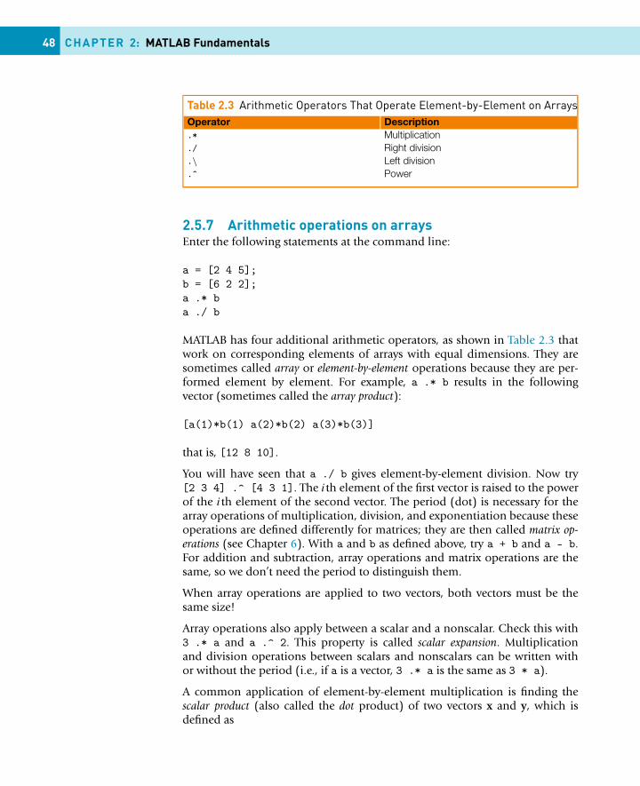
48 CHAPTER 2: MATLAB Fundamentals
Table 2.3 Arithmetic Operators That Operate Element-by-Element on ArraysOperator Description.* Multiplication./ Right division.\ Left division.ˆ Power
2.5.7 Arithmetic operations on arraysEnter the following statements at the command line:
a = [2 4 5];b = [6 2 2];a .* ba ./ b
MATLAB has four additional arithmetic operators, as shown in Table 2.3 thatwork on corresponding elements of arrays with equal dimensions. They aresometimes called array or element-by-element operations because they are per-formed element by element. For example, a .* b results in the followingvector (sometimes called the array product):
[a(1)*b(1) a(2)*b(2) a(3)*b(3)]
that is, [12 8 10].
You will have seen that a ./ b gives element-by-element division. Now try[2 3 4] .^ [4 3 1]. The ith element of the first vector is raised to the powerof the ith element of the second vector. The period (dot) is necessary for thearray operations of multiplication, division, and exponentiation because theseoperations are defined differently for matrices; they are then called matrix op-erations (see Chapter 6). With a and b as defined above, try a + b and a - b.For addition and subtraction, array operations and matrix operations are thesame, so we don’t need the period to distinguish them.
When array operations are applied to two vectors, both vectors must be thesame size!
Array operations also apply between a scalar and a nonscalar. Check this with3 .* a and a .^ 2. This property is called scalar expansion. Multiplicationand division operations between scalars and nonscalars can be written withor without the period (i.e., if a is a vector, 3 .* a is the same as 3 * a).
A common application of element-by-element multiplication is finding thescalar product (also called the dot product) of two vectors x and y, which isdefined as
2.5 Operators, expressions, and statements 49
x · y =∑
i
xiyi
The MATLAB function sum(z) finds the sum of the elements of the vector z,so the statement sum(a .* b) will find the scalar product of a and b (30 for aand b defined above).
Exercises
Use MATLAB array operations to do the following:
2.1. Add 1 to each element of the vector [2 3 -1].
2.2. Multiply each element of the vector [1 4 8] by 3.
2.3. Find the array product of the two vectors [1 2 3] and [0 -1 1]. (Answer:[0 -2 3])
2.4. Square each element of the vector [2 3 1].
2.5.8 ExpressionsAn expression is a formula consisting of variables, numbers, operators, andfunction names. It is evaluated when you enter it at the MATLAB prompt. Forexample, evaluate 2π as follows:
2 * pi
MATLAB’s response is
ans =6.2832
Note that MATLAB uses the function ans (which stands for answer) to returnthe last expression to be evaluated but not assigned to a variable.
If an expression is terminated with a semicolon (;), its value is not displayed,although it is still returned by ans.
2.5.9 StatementsMATLAB statements are frequently of the form
variable = expression
as in
s = u * t - g / 2 * t .^ 2;
50 CHAPTER 2: MATLAB Fundamentals
This is an example of an assignment statement because the value of the expres-sion on the right is assigned to the variable (s) on the left. Assignment alwaysworks in this direction. Note that the object on the left-hand side of the assign-ment must be a variable name. A common mistake is to get the statement thewrong way around, as in
a + b = c
Basically any line that you enter in the Command Window or in a program,which MATLAB accepts, is a statement, so a statement can be an assignment,a command, or simply an expression, such as
x = 29; % assignmentclear % commandpi/2 % expression
This naming convention is in keeping with most programming languages andserves to emphasize the different types of statements that are found in pro-gramming. However, the MATLAB documentation tends to refer to all of theseas “functions.”
As we have seen, a semicolon at the end of an assignment or expression sup-presses any output. This is useful for suppressing irritating output of interme-diate results (or large matrices).
A statement that is too long to fit on one line may be continued to the nextline with an ellipsis of at least three dots:
x = 3 * 4 - 8 ..../ 2 ^ 2;
Statements on the same line may be separated by commas (output not sup-pressed) or semicolons (output suppressed):
a = 2; b = 3, c = 4;
Note that the commas and semicolons are not technically part of the state-ments; they are separators.
Statements may involve array operations, in which case the variable on theleft-hand side may become a vector or a matrix.
2.5.10 Statements, commands, and functionsThe distinction between MATLAB statements, commands, and functions can bea little fuzzy, since all can be entered on the command line. However, it is
2.5 Operators, expressions, and statements 51
helpful to think of commands as changing the general environment in someway, for example, load, save, and clear. Statements do the sort of thing weusually associate with programming, such as evaluating expressions and car-rying out assignments, making decisions (if), and repeating (for). Functionsreturn with calculated values or perform some operation on data, such as sinand plot.
2.5.11 Formula vectorizationWith array operations, you can easily evaluate a formula repeatedly for a largeset of data. This is one of MATLAB’s most useful and powerful features, andyou should always look for ways to exploit it.
Let us again consider, as an example, the calculation of compound interest. Anamount of money A invested over a period of years n with an annual interestrate r grows to an amount A(1 + r)n. Suppose we want to calculate final bal-ances for investments of $750, $1000, $3000, $5000, and $11,999 over 10 yearswith an interest rate of 9%. The following program (comp.m) uses array opera-tions on a vector of initial investments to do this:
format bankA = [750 1000 3000 5000 11999];r = 0.09;n = 10;B = A * (1 + r) ^ n;disp( [A’ B’] )
The output is
750.00 1775.521000.00 2367.363000.00 7102.095000.00 11836.82
11999.00 28406.00
Note the following:
� In the statement B = A * (1 + r) ^ n, the expression (1 + r) ^ n isevaluated first because exponentiation has a higher precedence than multi-plication.
� Each element of the vector A is then multiplied by the scalar (1 + r) ^ n(scalar expansion).
� The operator * may be used instead of .* because the multiplication isbetween a scalar and a nonscalar (although .* would not cause an errorbecause a scalar is a special case of an array).
� A table is displayed whose columns are given by the transposes of A and B.
52 CHAPTER 2: MATLAB Fundamentals
This process is called formula vectorization. The operation in the statement de-scribed in bullet item 1 is such that every element in the vector B is determinedby operating on every element of vector A all at once, by interpreting once asingle command line.
See if you can adjust the program comp.m to find the balances for a singleamount A ($1000) over 1, 5, 10, 15, and 20 years. (Hint: use a vector for n:[1 5 10 15 20].)
Exercises2.1 Evaluate the following expressions yourself (before you use MATLAB to check).
The numerical answers are in parentheses.(a) 2 / 2 * 3 (3)(b) 2 / 3 ˆ 2 (2/9)(c) (2 / 3) ˆ 2 (4/9)(d) 2 + 3 * 4 - 4 (10)(e) 2 ˆ 2 * 3 / 4 + 3 (6)(f) 2 ˆ (2 * 3) / (4 + 3) (64/7)(g) 2 * 3 + 4 (10)(h) 2 ˆ 3 ˆ 2 (64)(i) - 4 ˆ 2 (-16; ˆ has higher precedence than -)
2.2 Use MATLAB to evaluate the following expressions. The answers are inparentheses.(a)
√2 (1.4142; use sqrt or ˆ0.5)
(b)3 + 4
5 + 6(0.6364; use brackets)
(c) Find the sum of 5 and 3 divided by their product (0.5333)(d) 232
(512)(e) Find the square of 2π (39.4784; use pi)(f) 2π2 (19.7392)(g) 1/
√2π (0.3989)
(h)1
2√
π(0.2821)
(i) Find the cube root of the product of 2.3 and 4.5 (2.1793)
(j)1 − 2
3+2
1 + 23−2
(0.2)
(k) 1000(1 + 0.15/12)60 (2107.2—for example, $1000 deposited for 5 years at15% per year, with the interest compounded monthly)
(l) (0.0000123 + 5.678 × 10−3) × 0.4567 × 10−4 (2.5988 × 10⁻⁷; use scientificnotation—for example, 1.23e-5 . . . ; do not use ˆ)
2.3 Try to avoid using unnecessary parentheses in an expression. Can you spot theerrors in the following expression? (Test your corrected version with MATLAB.)
(2(3+4)/(5*(6+1))^2
2.5 Operators, expressions, and statements 53
Note that the MATLAB Editor has two useful ways of dealing with the problemof “unbalanced delimiters” (which you should know about if you have beenworking through Help!):� When you type a closing delimiter, that is, a right ), ], or }, its matching
opening delimiter is briefly highlighted. So if you don’t see the highlightingwhen you type a right delimiter, you immediately know you’ve got one toomany.
� When you position the cursor anywhere inside a pair of delimiters andselect Text → Balance Delimiters (or press Ctrl+B), the characters insidethe delimiters are highlighted.
2.4 Set up a vector n with elements 1, 2, 3, 4, 5. Use MATLAB array operations on itto set up the following four vectors, each with five elements:(a) 2, 4, 6, 8, 10(b) 1/2, 1, 3/2, 2, 5/2(c) 1, 1/2, 1/3, 1/4, 1/5(d) 1,1/22,1/32,1/42,1/52
2.5 Suppose vectors a and b are defined as follows:
a = [2 -1 5 0];b = [3 2 -1 4];
Evaluate by hand the vector c in the following statements. Check your answerswith MATLAB.(a) c = a - b;(b) c = b + a - 3;(c) c = 2 * a + a .ˆ b;(d) c = b ./ a;(e) c = b . a;(f) c = a .ˆ b;(g) c = 2.ˆb+a;(h) c = 2*b/3.*a;(i) c = b*2.*a;
2.6 Water freezes at 32° and boils at 212° on the Fahrenheit scale. If C and F areCelsius and Fahrenheit temperatures, the formula
F = 9C/5 + 32
converts from one to the other. Use the MATLAB command line to convertCelsius 37° (normal human temperature) to Fahrenheit (98.6°).
2.7 Engineers often have to convert from one unit of measurement to another,which can be tricky sometimes. You need to think through the process carefully.For example, convert 5 acres to hectares, given that an acre is 4840 squareyards, a yard is 36 inches, an inch is 2.54 centimeters, and a hectare is 10,000square meters. The best approach is to develop a formula to convert x acres tohectares. You can do this as follows.� One square yard = (36×2.54)2 cm2
� So one acre = 4840 × (36 × 2.54)2 cm2
= 0.4047×108 cm2
= 0.4047 hectares
54 CHAPTER 2: MATLAB Fundamentals
� So x acres = 0.4047 × x hectaresOnce you have found the formula (but not before), MATLAB can do the rest:
x = 5; % acresh = 0.4047 * x; % hectaresdisp( h )
2.8 Develop formulae for the following conversions, and use some MATLABstatements to find the answers (in parentheses).(a) Convert 22 yards (an imperial cricket pitch) to meters. (20.117 meters)(b) One pound (weight) = 454 grams. Convert 75 kilograms to pounds.
(165.20 pounds)(c) Convert 49 meters/second (terminal velocity for a falling human-shaped
object) to kilometers per hour. (176.4 kilometers per hour)(d) One atmosphere pressure = 14.7 pounds per square inch (psi) =
101.325 kilo Pascals (kPa). Convert 40 psi to kPa. (275.71 kPa)(e) One calorie = 4.184 joules. Convert 6.25 kilojoules to calories.
(1.494 kilocalories)
2.6 OUTPUT
There are two straightforward ways of getting output from MATLAB:
� Entering a variable name, assignment, or expression on the command line,without a semicolon
� Using the disp statement (e.g., disp( x ))
2.6.1 The disp statementThe general form of disp for a numeric variable is
disp( variable }
When you use disp, the variable name is not displayed, and you don’t geta line feed before the value is displayed, as you do when you enter a variablename on the command line without a semicolon. disp generally gives a neaterdisplay.
You can also use disp to display a message enclosed in apostrophes (called astring). Apostrophes that are part of the message must be repeated:
disp( ’Pilate said, ’’What is truth?’’’ );
To display a message and a value on the same line, use the following trick:
x = 2;disp( [’The answer is ’, num2str(x)] );
2.6 Output 55
The output should be
The answer is 2
Square brackets create a vector, as we have seen. If we want to display a string,we create it; that is, we type a message between apostrophes. This we havedone already in the above example by defining the string ’The answer is ’.Note that the last space before the second apostrophe is part of the string. Allthe components of a MATLAB array must be either numbers or strings (unlessyou use a cell array—see Chapter 10), so we convert the number x to its stringrepresentation with the function num2str; read this as “number to string.”
You can display more than one number on a line as follows:
disp( [x y z] )
The square brackets create a vector with three elements, which are all displayed.
The command more on enables paging of output. This is very useful whendisplaying large matrices, for example, rand(100000,7) (see help more fordetails). If you forget to switch on more before displaying a huge matrix, youcan always stop the display with Ctrl+C.
As you gain experience with MATLAB you may wish to learn more about theinput and output capabilities in MATLAB. You can begin your search for in-formation by clicking the question mark at the top of the desktop to openthe help documents. Then search for fopen, a utility which allows you toopen a file. Scroll to the bottom of the page in the help manual on this topicand find the following list of functions: fclose, feof, ferror, fprintf,fread, fscanf, fseek, ftell, fwrite. Click on fprintf, which is a for-matted output utility that is popular if you are a C-language programmer.Search for input in the help manual to learn more about this function thatis used in a number of examples in this text. Of course, the simplest input ofdata is the assignment of values to variables in a program of commands.
2.6.2 The format commandThe term format refers to how something is laid out: in this case MATLAB out-put. The default format in MATLAB has the following basic output rules:
� It always attempts to display integers (whole numbers) exactly. However, ifthe integer is too large, it is displayed in scientific notation with five signif-icant digits—1234567890 is displayed as 1.2346e+009 (i.e., 1.2346 × 10⁹).Check this by first entering 123456789 at the command line and then1234567890.
� Numbers with decimal parts are displayed with four significant digits. Ifthe value x is in the range 0.001 < x ≤ 1000, it is displayed in fixed-point form; otherwise, scientific (floating-point) notation is used, in which
56 CHAPTER 2: MATLAB Fundamentals
case the mantissa is between 1 and 9.9999 (e.g., 1000.1 is displayed as1.0001e+003). Check this by entering the following numbers at the prompt(on separate lines): 0.0011, 0.0009, 1/3, 5/3, 2999/3, 3001/3.
You can change from the default with variations on the format command,as follows. If you want values displayed in scientific notation (floating-pointform) whatever their size, enter the command
format short e
All output from subsequent disp statements will be in scientific notation, withfive significant digits, until the next format command is issued. Enter this com-mand and check it with the following values: 0.0123456, 1.23456, 123.456 (allon separate lines).
If you want more accurate output, you can use format long e. This alsogives scientific notation but with 15 significant digits. Try it out on 1/7. Useformat long to get fixed-point notation with 15 significant digits. Try 100/7and pi. If you’re not sure of the order of magnitude of your output you cantry format short g or format long g. The g stands for “general.” MATLABdecides in each case whether to use fixed or floating point.
Use format bank for financial calculations; you get fixed point with two dec-imal digits (for cents). Try it on 10000/7. Suppress irritating line feeds withformat compact, which gives a more compact display. format loose revertsto a more airy display. Use format hex to get hexadecimal display.
Use format rat to display a number as a rational approximation (ratio of twointegers). For example, pi is displayed as 355/113, a pleasant change from thetired old 22/7. Note that even this is an approximation! Try out format raton
√2 and e (exp(1)).
The symbols +, −, and a space are displayed for positive, negative, and zeroelements of a vector or matrix after the command format +. In certain appli-cations this is a convenient way of displaying matrices. The command formatby itself reverts to the default format. You can always try help format if you’reconfused!
2.6.3 Scale factorsEnter the following commands (MATLAB’s response is also shown).
� format compact
� x = [1e3 1 1e-4]
x =
1.0e+003 *
1.0000 0.0010 0.0000
2.7 Repeating with for 57
With format short (the default) and format long, a common scale factor isapplied to the whole vector if its elements are very large or very small or differgreatly in magnitude. In this example, the common scale factor is 1000, so theelements displayed must all be multiplied by it to get their proper value—forexample, for the second element 1.0e+003 * 0.0010 gives 1. Taking a factorof 1000 out of the third element (1e-4) leaves 1e-7, which is represented by0.0000 since only four decimal digits are displayed.
If you don’t want a scale factor, try format bank or format short e:
�x
x =
1000.0000 1.00 0.00
�format short e
�x
x =
1.0000e+003 1.0000e+000 1.0000e-004
2.7 REPEATING WITH for
So far we have seen how to get data into a program (i.e., provide input), howto do arithmetic, and how to get some results (i.e., get output). In this sectionwe look at a new feature: repetition. This is implemented by the extremelypowerful for construct. We will first look at some examples of its use, followedby explanations.
For starters, enter the following group of statements on the command line.Enter the command format compact first to make the output neater:
for i = 1:5, disp(i), end
Now change it slightly to
for i = 1:3, disp(i), end
And what about
for i = 1:0, disp(i), end
Can you see what’s happening? The disp statement is repeated five times, threetimes, and not at all.
58 CHAPTER 2: MATLAB Fundamentals
2.7.1 Square roots with Newton’s methodThe square root x of any positive number a may be found using only the arith-metic operations of addition, subtraction, and division with Newton’s method.This is an iterative (repetitive) procedure that refines an initial guess.
To introduce in a rather elementary way the notion of structured programming(to be described in more detail in Chapter 3), let us consider the structure planof the algorithm to find a square root and a program with sample output fora = 2.
Here is the structure plan:
1. Initialize a
2. Initialize x to a/23. Repeat 6 times (say) the following:
Replace x by (x + a/x)/2Display x
4. Stop
Here is the program:
a = 2;x = a/2;disp([’The approach to sqrt(a) for a = ’, num2str(a)])
for i = 1:6x = (x + a / x) / 2;disp( x )
end
disp( ’Matlab’’s value: ’ )disp( sqrt(2) )
Here is the output (after selecting format long):
The approach to sqrt(a) for a = 21.500000000000001.416666666666671.414215686274511.414213562374691.414213562373101.41421356237310
Matlab’s value:1.41421356237310
2.7 Repeating with for 59
The value of x converges to a limit rather quickly in this case,√
a. Note that itis identical to the value returned by MATLAB’s sqrt function. Most computersand calculators use a similar method internally to compute square roots andother standard mathematical functions.
The general form of Newton’s method is presented in Chapter 14.
2.7.2 Factorials!Run the following program to generate a list of n and n! (“n factorial,” or “nshriek”), where
n! = 1 × 2 × 3 × . . . × (n − 1) × n (2.1)
n = 10;fact = 1;for k = 1:n
fact = k * fact;disp( [k fact] )
end
Experiment to find the largest value of n for which MATLAB can find the n
factorial. (You had better leave out the disp statement! Or you can move itfrom above the end command to below it.)
2.7.3 Limit of a sequencefor loops are ideal for computing successive members of a sequence (as inNewton’s method). The following example also highlights a problem thatsometimes occurs when computing a limit. Consider the sequence
xn = an
n! , n = 1,2,3 . . .
where a is any constant and n! is the factorial function defined above. Thequestion is this: What is the limit of this sequence as n gets indefinitely large?Let’s take the case a = 10. If we try to compute xn directly, we can get intotrouble, because n! grows very rapidly as n increases, and numerical overflowcan occur. However, the situation is neatly transformed if we spot that xn isrelated to xn−1 as follows:
xn = axn−1
n.
There are no numerical problems now.
The following program computes xn for a = 10 and increasing values of n.
a = 10;x = 1;
60 CHAPTER 2: MATLAB Fundamentals
k = 20; % number of terms
for n = 1:kx = a * x / n;disp( [n x] )
end
2.7.4 The basic for constructIn general the most common form of the for loop (for use in a program, noton the command line) is
for index = j:kstatements;
end
or
for index = j:m:kstatements;
end
Note the following points carefully:
� j:k is a vector with elements j, j + 1, j + 2, . . . , k.� j:m:k is a vector with elements j, j + m,j + 2m, . . . , such that the last
element does not exceed k if m > 0 or is not less than k if m < 0.� index must be a variable. Each time through the loop it will contain the next
element of the vector j:k or j:m:k, and statements (there may be one ormore) are carried out for each of these values.If the for construct has the form
for k = first:increment:last
The number of times the loop is executed may be calculated from the fol-lowing equation:
floor(last− firstincrement
)+ 1
where the MATLAB function floor(x) rounds x down toward −∞. Thisvalue is called the iteration or trip count. As an example, let us consider thestatement for i = 1:2:6. It has an iteration count of
floor(
6 − 1
2
)+ 1 = floor
(5
2
)+ 1 = 3
Thus i takes the values 1, 3, 5. Note that if the iteration count is negative,the loop is not executed.
2.7 Repeating with for 61
� On completion of the for loop the index contains the last value used.� If the vector j:k or j:m:k is empty, statements are not executed and control
passes to the statement following end.� The index does not have to appear explicitly in statements. It is basically
a counter. In fact, if the index does appear explicitly in statements, the forcan often be vectorized (more details on this are given in Section 2.7.7).A simple example of a more efficient (faster) program is as follows. Theexamples with disp at the beginning of this section were for illustrationonly; strictly, it would be more efficient to say (without “for”)
i = 1:5; disp( i’ )
Can you see the difference? In this case i is assigned as a vector (hence, thischange vectorizes the original program).
� It is good programming style to indent (tabulate) the statements inside afor loop. You may have noticed that the Editor does this for you automat-ically with a feature called smart indenting.
2.7.5 for in a single lineIf you insist on using for in a single line, here is the general form:
for index = j:k; statements; end
or
for index = j:m:k; statements; end
Note the following:
� Don’t forget the commas (semicolons will also do if appropriate). If youleave them out you will get an error message.
� Again, statements can be one or more statements separated by commas orsemicolons.
� If you leave out end, MATLAB will wait for you to enter it. Nothing willhappen until you do so.
2.7.6 More general forA more general form of for is
for index = v
where v is any vector. The index moves through each element of the vector inturn, providing a neat way of processing each item in a list. Other forms of thefor loop as well as the while loop will be discussed in Chapter 8.
62 CHAPTER 2: MATLAB Fundamentals
2.7.7 Avoid for loops by vectorizing!There are situations where a for loop is essential, as in many of the examplesin this section so far. However, given the way MATLAB has been designed, forloops tend to be inefficient in terms of computing time. If you have written afor loop that involves the index of the loop in an expression, it may be possi-ble to vectorize the expression, making use of array operations where necessary,as the following examples show.
Suppose you want to evaluate
1 00 000∑n=1
n
(and can’t remember the formula for the sum). Here’s how to do it with a forloop (run the program, which also times how long it takes):
t0 = clock;s = 0;for n = 1:100000
s = s + n;endetime(clock, t0)
The MATLAB function clock returns a six-element vector with the current dateand time in the format year, month, day, hour, minute, seconds. Thus, t0records when the calculation starts.
The function etime returns the time in seconds elapsed between its two ar-guments, which must be vectors as returned by clock. On a Pentium II, itreturned about 3.35 seconds, which is the total time for this calculation. (Ifyou have a faster PC, it should take less time.)
Now try to vectorize this calculation (before looking at the solution). Here it is:
t0 = clock;n = 1:100000;s = sum( n );etime(clock, t0)
This way takes only 0.06 seconds on the same PC—more than 50 times faster!
There is a neater way of monitoring the time taken to interpret MATLAB state-ments: the tic and toc function. Suppose you want to evaluate
1 00 000∑n=1
1
n2
Here’s the for loop version:
2.7 Repeating with for 63
tics = 0;for n = 1:100000
s = s + 1/n^2;endtoc
which takes about 6 seconds on the same PC. Once again, try to vectorize thesum:
ticn = 1:100000;s = sum( 1./n.^2 );toc
The same PC gives a time of about 0.05 seconds for the vectorized version—more than 100 times faster! (Of course, the computation time in these ex-amples is small regardless of the method applied. However, learning how toimprove the efficiency of computation to solve more complex scientific or en-gineering problems will be helpful as you develop good programming skills.More details on good problem-solving and program design practices are intro-duced at the end of this chapter and dealt with, in more detail, in the next.)
Series with alternating signs are a little more challenging. This series sums toln(2) (the natural logarithm of 2):
1 − 1
2+ 1
3− 1
4+ 1
5− · · ·
Here’s how to find the sum of the first 9999 terms with a for loop (note howto handle the alternating sign):
sign = -1;s = 0;
for n = 1:9999sign = -sign;
s = s + sign / n;end
Try it. You should get 0.6932. MATLAB’s log(2) gives 0.6931. Not bad.
The vectorized version is as follows:
n = 1:2:9999;s = sum( 1./n - 1./(n+1) )
64 CHAPTER 2: MATLAB Fundamentals
If you time the two versions, you will again find that the vectorized form ismany times faster.
MATLAB’s functions naturally exploit vectorization wherever possible. For ex-ample, prod(1:n) will find n! much faster than the code at the beginning ofthis section (for large values of n).
Exercises
Write MATLAB programs to find the following sums with for loops and byvectorization. Time both versions in each case.
� 12 + 22 + 32 + · · · + 1 0002 (sum is 333 833 500)
� 1 − 1
3+ 1
5− 1
7+ 1
9− · · · − 1
1003(sum is 0.7849—converges slowly to π /4)
� Sum the left-hand side of the series
1
12 · 32+ 1
32 · 52+ 1
52 · 72+ · · · = π2 − 8
16(sum is 0.1169—with 500 terms)
2.8 DECISIONS
The MATLAB function rand generates a random number in the range 0–1.Enter the following two statements at the command line:
r = randif r > 0.5 disp( ’greater indeed’ ), end
MATLAB should only display the message greater indeed if r is in fact greaterthan 0.5 (check by displaying r). Repeat a few times—cut and paste from theCommand History window (make sure that a new r is generated each time).
As a slightly different but related exercise, enter the following logical expressionon the command line:
2 > 0
Now enter the logical expression -1 > 0. MATLAB gives a value of 1 to a logicalexpression that is true and 0 to one that is false.
2.8.1 The one-line if statementIn the last example MATLAB has to make a decision; it must decide whetheror not r is greater than 0.5. The if construct, which is fundamental to allcomputing languages, is the basis of such decision making. The simplest formof if in a single line is
if condition; statements; end
2.8 Decisions 65
Table 2.4 Relational OperatorsRelational operator Meaning< less than<= less than or equal== equal~= not equal> greater than>= greater than or equal
Note the following points:
� condition is usually a logical expression (i.e., it contains a relational operator),which is either true or false. The relational operators are shown in Table 2.4.MATLAB allows you to use an arithmetic expression for condition. If theexpression evaluates to 0, it is regarded as false; any other value is true. Thisis not generally recommended; the if statement is easier to understand (foryou or a reader of your code) if condition is a logical expression.
� If condition is true, statement is executed, but if condition is false, nothinghappens.
� condition may be a vector or a matrix, in which case it is true only if all of itselements are nonzero. A single zero element in a vector or matrix renders itfalse.
if condition statement, end
Here are more examples of logical expressions involving relational operators,with their meanings in parentheses:
b^2 < 4*a*c (b2 < 4ac)
x >= 0 (x ≥ 0)a ~= 0(a = 0)b^2 == 4*a*c (b2 = 4ac)
Remember to use the double equal sign (==) when testing for equality:
if x == 0; disp( ’x equals zero’); end
Exercises
The following statements all assign logical expressions to the variable x. See if youcan correctly determine the value of x in each case before checking your answer withMATLAB.
(a) x = 3 > 2
66 CHAPTER 2: MATLAB Fundamentals
(b) x = 2 > 3(c) x = -4 <= -3(d) x = 1 < 1(e) x = 2 ~= 2(f) x = 3 == 3(g) x = 0 < 0.5 < 1
Did you get item (f)? 3 == 3 is a logical expression that is true since 3 is undoubtedlyequal to 3. The value 1 (for true) is therefore assigned to x. After executing thesecommands type the command whos to find that the variable x is in the class of logicalvariables.
What about (g)? As a mathematical inequality,
0 < 0.5 < 1
is undoubtedly true from a nonoperational point of view. However, as a MATLAB oper-ational expression, the left-hand < is evaluated first, 0 < 0.5, giving 1 (true). Then theright-hand operation is performed, 1 < 1, giving 0 (false). Makes you think, doesn’t it?
2.8.2 The if-else constructIf you enter the two lines
x = 2;if x < 0 disp( ’neg’ ), else disp( ’non-neg’), end
do you get the message non-neg? If you change the value of x to −1 and executethe if again, do you get the message neg this time? Finally, if you try
if 79 disp( ’true’ ), else disp(’false’ ), end
do you get true? Try other values, including 0 and some negative values.
Most banks offer differential interest rates. Suppose the rate is 9% if theamount in your savings account is less than $5000, but 12% otherwise. TheRandom Bank goes one step further and gives you a random amount in youraccount to start with! Run the following program a few times:
bal = 10000 * rand;
if bal < 5000rate = 0.09;
elserate = 0.12;
end
2.8 Decisions 67
newbal = bal + rate * bal;disp( ’New balance after interest compounded is:’ )format bankdisp( newbal )
Display the values of bal and rate each time from the command line to checkthat MATLAB has chosen the correct interest rate.
The basic form of if-else for use in a program file is
if conditionstatementsA
elsestatementsB
end
Note that
� statementsA and statementsB represent one or more statements.� If condition is true, statementsA are executed, but if condition is false, state-
mentsB are executed. This is essentially how you force MATLAB to choosebetween two alternatives.
� else is optional.
2.8.3 The one-line if-else statementThe simplest general form of if-else for use on one line is
if condition; statementA; else; statementB; end
Note the following:
� Commas (or semicolons) are essential between the various clauses.� else is optional.� end is mandatory; without it, MATLAB will wait forever.
2.8.4 elseifSuppose the Random Bank now offers 9% interest on balances of less than$5000, 12% for balances of $5000 or more but less than $10,000, and 15%for balances of $10,000 or more. The following program calculates a customer’snew balance after one year according to this scheme:
bal = 15000 * rand;
if bal < 5000rate = 0.09;
68 CHAPTER 2: MATLAB Fundamentals
elseif bal < 10000rate = 0.12;
elserate = 0.15;
end
newbal = bal + rate * bal;format bankdisp( ’New balance is:’ )disp( newbal )
Run the program a few times, and once again display the values of bal andrate each time to convince yourself that MATLAB has chosen the correct inter-est rate.
In general, the elseif clause is used:
if condition1statementsA
elseif condition2statementsB
elseif condition3statementsC
...else
statementsEend
This is sometimes called an elseif ladder. It works as follows:
1. condition1 is tested. If it is true, statementsA are executed; MATLAB thenmoves to the next statement after end.
2. If condition1 is false, MATLAB checks condition2. If it is true, statementsB areexecuted, followed by the statement after end.
3. In this way, all conditions are tested until a true one is found. As soon asa true condition is found, no further elseifs are examined and MATLABjumps off the ladder.
4. If none of the conditions is true, statements after else are executed.5. Arrange the logic so that not more than one of the conditions is true.6. There can be any number of elseifs, but at most one else.7. elseif must be written as one word.8. It is good programming style to indent each group of statements as shown.
2.8.5 Logical operatorsMore complicated logical expressions can be constructed using the three logicaloperators: & (and), | (or), and ~ (not). For example, the quadratic equation
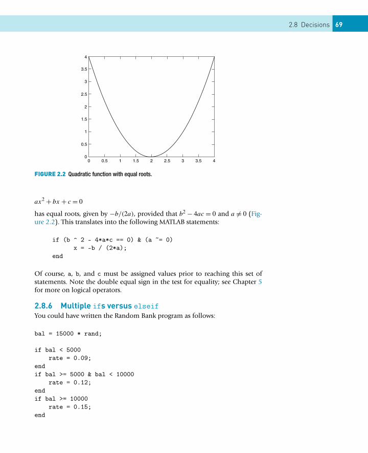
2.8 Decisions 69
FIGURE 2.2 Quadratic function with equal roots.
ax2 + bx + c = 0
has equal roots, given by −b/(2a), provided that b2 − 4ac = 0 and a = 0 (Fig-ure 2.2). This translates into the following MATLAB statements:
if (b ^ 2 - 4*a*c == 0) & (a ~= 0)x = -b / (2*a);
end
Of course, a, b, and c must be assigned values prior to reaching this set ofstatements. Note the double equal sign in the test for equality; see Chapter 5for more on logical operators.
2.8.6 Multiple ifs versus elseifYou could have written the Random Bank program as follows:
bal = 15000 * rand;
if bal < 5000rate = 0.09;
endif bal >= 5000 & bal < 10000
rate = 0.12;endif bal >= 10000
rate = 0.15;end
70 CHAPTER 2: MATLAB Fundamentals
newbal = bal + rate * bal;format bankdisp( ’New balance is’ )disp( newbal )
However, this is inefficient since each of the three conditions is always tested,even if the first one is true. In the earlier elseif version, MATLAB jumps off theelseif ladder as soon as it finds a true condition. This saves a lot of computingtime (and is easier to read) if the if construct is in a loop that is repeated often.
Using this form, instead of the elseif ladder, you can make the followingcommon mistake:
if bal < 5000rate = 0.09;
endif bal < 10000
rate = 0.12;endif bal >= 10000
rate = 0.15;end
Can you see why you get the wrong answer (1120 instead of 1090) if bal hasthe value 1000? When designing the logic, you need to make sure that one andonly one of the conditions will be true at any one time.
Another mistake frequently made is to replace the second if with somethinglike
if 5000 < bal < 10000rate = 0.12;
end
which is compelling, as we saw above. However, whatever the value of bal, thiscondition will always be true. Can you see why? (Note that if bal is greater than5000—for example, bal = 20000—the numerical truth value of the first test,namely, 5000 < bal, is true and hence has the numerical value of 1 since 1 isalways less than 10000, even if bal = 20000.)
2.8.7 Nested ifsAn if construct can contain further ifs and so on. This is called nesting andshould not be confused with the elseif ladder. You have to be careful withelses. In general, else belongs to the most recent if that has not been ended.
2.8 Decisions 71
The correct positioning of end is therefore very important, as the next exampledemonstrates.
Suppose you want to compute the solution to a quadratic equation. You maywant to check whether a = 0 to prevent a division by zero. Your program couldcontain the following nested ifs:
...d = b ^ 2 - 4*a*c;if a ~= 0
if d < 0disp( ’Complex roots’ )
elsex1 = (-b + sqrt( d )) / (2*a);x2 = (-b - sqrt( d )) / (2*a);
end % first end <<<<<<<<<<<<end
The else belongs to the second if by default, as intended.
Now move the first end up as follows:
d = b ^ 2 {-} 4*a*c;if a $^\sim$= 0
if d < 0disp( ’Complex roots’ )
end \% first end moved up now <<<<<<<<<<<<else
x1 = (-b + sqrt( d )) / (2*a);x2 = (-b {-} sqrt( d )) / (2*a);
end
The end that has been moved now closes the second if. The result is that elsebelongs to the first if instead of to the second one. Division by zero is thereforeguaranteed instead of prevented!
2.8.8 Vectorizing ifs?You may be wondering if for statements enclosing ifs can be vectorized. Theanswer is yes, courtesy of logical arrays. Discussion of this rather interestingtopic is postponed until Chapter 5.
2.8.9 The switch statementswitch executes certain statements based on the value of a variable or expres-sion. In this example it is used to decide whether a random integer is 1, 2, or3 (see Section 5.1.5 for an explanation of this use of rand):
72 CHAPTER 2: MATLAB Fundamentals
d = floor(3*rand) + 1switch dcase 1
disp( ’That’’s a 1!’ );case 2
disp( ’That’’s a 2!’ );otherwise
disp( ’Must be 3!’ );end
Multiple expressions can be handled in a single case statement by enclosingthe case expression in a cell array (see Chapter 10):
d = floor(10*rand);switch dcase {2, 4, 6, 8}
disp( ’Even’ );case {1, 3, 5, 7, 9}
disp( ’Odd’ );otherwise
disp( ’Zero’ );end
2.9 COMPLEX NUMBERS
If you are not familiar with complex numbers, you can safely skip this section.However, it is useful to know what they are since the square root of a negativenumber may come up as a mistake if you are trying to work only with realnumbers.
It is very easy to handle complex numbers in MATLAB. The special values iand j stand for
√−1. Try sqrt(-1) to see how MATLAB represents complexnumbers.
The symbol i may be used to assign complex values, for example,
z = 2 + 3*i
represents the complex number 2 + 3i (real part 2, imaginary part 3). You canalso input a complex value like this:
2 + 3*i
in response to the input prompt (remember, no semicolon). The imaginarypart of a complex number may also be entered without an asterisk, 3i.
2.9 Complex numbers 73
All of the arithmetic operators (and most functions) work with complex num-bers, such as sqrt(2 + 3*i) and exp(i*pi). Some functions are specific tocomplex numbers. If z is a complex number, real(z), imag(z), conj(z), andabs(z) all have the obvious meanings.
A complex number may be represented in polar coordinates:
z = reiθ
angle(z) returns θ between −π and π ; that is, atan2(imag(z), real(z)).abs(z) returns the magnitude r .
Since eiθ gives the unit circle in polars, complex numbers provide a neat wayof plotting a circle. Try the following:
circle = exp( 2*i*[1:360]*pi/360 );plot(circle)axis(’equal’)
Note these points:
� If y is complex, the statement plot(y) is equivalent to
plot(real(y), imag(y))
� The statement axis(’equal’) is necessary to make circles look round; itchanges what is known as the aspect ratio of the monitor. axis(’normal’)gives the default aspect ratio.
If you are using complex numbers, be careful not to use i or j for othervariables; the new values will replace the value of
√−1 and will cause nastyproblems.
For complex matrices, the operations ’ and .’ behave differently. The ’ op-erator is the complex conjugate transpose, meaning rows and columns are inter-changed and signs of imaginary parts are changed. The .’ operator, on theother hand, does a pure transpose without taking the complex conjugate. Tosee this, set up a complex matrix a with the statement
a = [1+i 2+2i; 3+3i 4+4i]
which results in
a =1.0000 + 1.0000i 2.0000 + 2.0000i3.0000 + 3.0000i 4.0000 + 4.0000i
The statement
74 CHAPTER 2: MATLAB Fundamentals
a’
then results in the complex conjugate transpose
ans =1.0000 - 1.0000i 3.0000 - 3.0000i2.0000 - 2.0000i 4.0000 - 4.0000i
whereas the statement
a.’
results in the pure transpose
ans =1.0000 + 1.0000i 3.0000 + 3.0000i2.0000 + 2.0000i 4.0000 + 4.0000i
SUMMARY� The MATLAB desktop consists of a number of tools: the Command Win-
dow, the Workspace browser, the Current Directory browser, and the Com-mand History window.
� MATLAB has a comprehensive online Help system. It can be accessedthrough the Help button (?) on the desktop toolbar or the Help menu inany tool.
� A MATLAB program can be written in the Editor and cut and pasted to theCommand Window (or it can be executed from the editor by clicking thegreen right arrow in the toolbar at the top of the Editor window).
� A script file is a text file (created by the MATLAB Editor or any other texteditor) containing a collection of MATLAB statements. In other words, itis a program. The statements are carried out when the script file name isentered at the prompt in the Command Window. A script file name musthave the .m extension. Script files are therefore also called M-files.
� The recommended way to run a script is from the Current Directorybrowser. The output from the script will then appear in the Command Win-dow.
� A variable name consists only of letters, digits, and underscores, and muststart with a letter. Only the first 63 characters are significant. MATLAB iscase-sensitive by default. All variables created during a session remain in theworkspace until removed with clear. The command who lists the variablesin the workspace; whos gives their sizes.
� MATLAB refers to all variables as arrays, whether they are scalars (single-valued arrays), vectors, (1D arrays), or matrices (2D arrays).
2.9 Summary 75
� MATLAB names are case-sensitive.� The Workspace browser on the desktop provides a handy visual represen-
tation of the workspace. Clicking a variable in it invokes the Array Editor,which may be used to view and change variable values.
� Vectors and matrices are entered in square brackets. Elements are separatedby spaces or commas. Rows are separated by semicolons. The colon oper-ator is used to generate vectors, with elements increasing (decreasing) byregular increments (decrements). Vectors are row vectors by default. Usethe apostrophe transpose operator (’) to change a row vector into a col-umn vector.
� An element of a vector is referred to by a subscript in parentheses. A sub-script may itself be a vector. Subscripts always start at 1.
� The diary command copies everything that subsequently appears in theCommand Window to the specified text file until the command diary offis given.
� Statements on the same line may be separated by commas or semicolons.� A statement may be continued to the next line with an ellipsis of at least
three dots.� Numbers may be represented in fixed-point decimal notation or in floating-
point scientific notation.� MATLAB has 14 data types. The default numeric type is double precision.
All mathematical operations are carried out in double precision.� The six arithmetic operators for scalars are +, -, *, \, /, and ^. They
operate according to rules of precedence.� An expression is a rule for evaluating a formula using numbers, operators,
variables, and functions. A semicolon after an expression suppresses displayof its value.
� Array operations are element by element between vectors or between scalarsand vectors. The array operations of multiplication, right and left division,and exponentiation are indicated by .*, ./, .\, and .^ to distinguishthem from vector and matrix operations of the same name. They may beused to evaluate a formula repeatedly for some or all of the elements of avector. This is called vectorization of the formula.
� disp is used to output (display) numbers and strings. num2str is usefulwith disp for displaying strings and numbers on the same line.
� The format command controls the way output is displayed.� When vectors are displayed, a common scale factor is used if the elements
are very large or very small, or differ greatly in magnitude.� The for statement is used to repeat a group of statements a fixed num-
ber of times. If the index of a for statement is used in the expression beingrepeated, the expression can often be vectorized, saving a great deal of com-puting time.
� tic and toc may be used as a stopwatch.� Logical expressions have the value true (1) or false (0) and are constructed
with the six relational operators >, >=, <, <=, ==, and ~=. Any ex-
76 CHAPTER 2: MATLAB Fundamentals
pression that evaluates to zero is regarded as false. Any other value is true.More complicated logical expressions can be formed from other logical ex-pressions using the logical operators & (and), | (or), and ~ (not).
� if–else executes different groups of statements according to whether a log-ical expression is true or false. The elseif ladder is a good way to choosebetween a number of options, only one of which should be true at a time.
� switch enables choices to be made between discrete cases of a variable orexpression.
� A string is a collection of characters enclosed in apostrophes.� Complex numbers may be represented using the special variables i and j,
which stand for the unit imaginary number√−1.
EXERCISES2.1 Decide which of the following numbers are not acceptable in MATLAB,
and state why:(a) 9,87(b) .0(c) 25.82(d) -356231(e) 3.57*e2(f) 3.57e2.1(g) 3.57e+2(h) 3,57e-2
2.2 State, giving reasons, which of the following are not valid MATLAB vari-able names:(a) a2(b) a.2(c) 2a(d) ’a’one(e) aone(f) _x_1(g) miXedUp(h) pay day(i) inf(j) Pay_Day(k) min*2(l) what
2.3 Translate the following expressions into MATLAB:
(a) p + w
u
(b) p + w
u + v
(c)p + w
u+v
p + wu−v
2.9 Exercises 77
(d) x1/2
(e) yy+z
(f) xyz
(g) (xy)z
(h) x − x3/3! + x5/5!2.4 Translate the following into MATLAB statements:
(a) Add 1 to the value of i and store the result in i.(b) Cube i, add j to this, and store the result in i.(c) Set g equal to the larger of the two variables e and f.(d) If d is greater than 0, set x equal to −b.(e) Divide the sum of a and b by the product of c and d, and store the
result in x.2.5 What’s wrong with the following MATLAB statements?
(a) n + 1 = n;(b) Fahrenheit temp = 9*C/5 + 32;(c) 2 = x;
2.6 Write a program to calculate x, where
x = −b + √b2 − 4ac
2a
and a = 2, b = −10, c = 12 (Answer 3.0)2.7 There are eight pints in a gallon and 1.76 pints in a liter. The volume of
a tank is given as 2 gallons and 4 pints. Write a script that inputs thisvolume in gallons and pints and converts it to liters. (Answer: 11.36)
2.8 Write a program to calculate gasoline consumption. It should assign thedistance traveled (in kilometers) and the amount of gas used (in liters)and compute the consumption in km/liter as well as in the more usualform of liters/100 km. Write some helpful headings so that your outputlooks something like this:
Distance Liters used km/L L/100km528 46.23 11.42 8.76
2.9 Write some statements in MATLAB that exchange the contents of twovariables a and b, using only one additional variable t.
2.10 Try Exercise 2.9 without using any additional variables!2.11 If C and F are Celsius and Fahrenheit temperatures, respectively, the
formula for conversion from Celsius to Fahrenheit is F = 9C/5 + 32.(a) Write a script that will ask you for the Celsius temperature and dis-
play the Fahrenheit equivalent with some sort of comment, such as
The Fahrenheit temperature is:...
Try it out on the following Celsius temperatures (answers in paren-theses): 0 (32), 100 (212), −40 (−40!), 37 (normal human temper-ature: 98.6).
78 CHAPTER 2: MATLAB Fundamentals
(b) Change the script to use vectors and array operations to compute theFahrenheit equivalents of Celsius temperatures ranging from 20◦ to30◦ in steps of 1◦, and display them in two columns with a heading,like this:
Celsius Fahrenheit20.00 68.0021.00 69.80...30.00 86.00
2.12 Generate a table of conversions from degrees (first column) to radians(second column). Degrees should go from 0◦ to 360◦ in steps of 10◦.Recall that π radians = 180◦.
2.13 Set up a matrix (table) with degrees in the first column from 0 to 360 insteps of 30, sines in the second column, and cosines in the third column.Now try to add tangents in the fourth column. Can you figure out what’sgoing on? Try some variations of the format command.
2.14 Write some statements that display a list of integers from 10 to 20 inclu-sive, each with its square root next to it.
2.15 Write a single statement to find and display the sum of the successiveeven integers 2, 4, . . . , 200. (Answer: 10,100)
2.16 Ten students in a class take a test. The marks are out of 10. All the marksare entered in a MATLAB vector, marks. Write a statement to find anddisplay the average mark. Try it on the following:
5 8 0 10 3 8 5 7 9 4 (Answer: 5.9)
Hint: Use the mean function.2.17 What are the values of x and a after the following statements have been
executed?(a) a = 0;(b) i = 1;(c) x = 0;(d) a = a + i;(e) x = x + i / a;(f) a = a + i;(g) x = x + i / a;(h) a = a + i;(i) x = x + i / a;(j) a = a + i;(k) x = x + i / a;
2.18 Rewrite the statements in Exercise 2.17 more economically by using afor loop. Can you do even better by vectorizing the code?
2.9 Exercises 79
2.19 Work out by hand the output of the following script for n = 4:
n = input( ’Number of terms? ’ );s = 0;
for k = 1:ns = s + 1 / (k ^ 2);
end;disp(sqrt(6 * s))
If you run this script for larger and larger values of n, you will find thatthe output approaches a well-known limit. Can you figure out what itis? Now rewrite the script using vectors and array operations.
2.20 Work through the following script by hand. Draw up a table of the valuesof i, j, and m to show how they change while the script executes. Checkyour answers by running the script.
v = [3 1 5];i = 1;
for j = vi = i + 1;if i == 3
i = i + 2;m = i + j;
endend
2.21 The steady-state current I flowing in a circuit that contains a resistanceR = 5, capacitance C = 10, and inductance L = 4 in series is given by
I = E√R2 + (2πωL − 1−
2πωC− )2
where E = 2 and ω = 2 are the input voltage and angular frequency,respectively. Compute the value of I . (Answer: 0.0396)
2.22 The electricity accounts of residents in a very small town are calculatedas follows:� If 500 units or fewer are used, the cost is 2 cents per unit.� If more than 500 but not more than 1000 units are used, the cost is
$10 for the first 500 units and 5 cents for every unit in excess of 500.� If more than 1000 units are used, the cost is $35 for the first 1000
units plus 10 cents for every unit in excess of 1000.� A basic service fee of $5 is charged, no matter how much electricity is
used.Write a program that enters the following five consumptions into a vec-tor and uses a for loop to calculate and display the total charge for eachone: 200, 500, 700, 1000, 1500. (Answers: $9, $15, $25, $40, $90)
80 CHAPTER 2: MATLAB Fundamentals
2.23 Suppose you deposit $50 in a bank account every month for a year. Everymonth, after the deposit has been made, interest at the rate of 1% isadded to the balance: After one month the balance is $50.50, and aftertwo months it is $101.51. Write a program to compute and print thebalance each month for a year. Arrange the output to look somethinglike this:
MONTH MONTH-END BALANCE
1 50.502 101.513 153.02...
12 640.47
2.24 If you invest $1000 for one year at an interest rate of 12%, the return is$1120 at the end of the year. But if interest is compounded at the rateof 1% monthly (i.e., 1/12 of the annual rate), you get slightly more inter-est because it is compounded. Write a program that uses a for loop tocompute the balance after a year of compounding interest in this way.The answer should be $1126.83. Evaluate the formula for this result sep-arately as a check: 1000 × 1.0112.
2.25 A plumber opens a savings account with $100,000 at the beginning ofJanuary. He then makes a deposit of $1000 at the end of each month forthe next 12 months (starting at the end of January). Interest is calculatedand added to his account at the end of each month (before the $1000deposit is made). The monthly interest rate depends on the amount A
in his account at the time interest is calculated, in the following way:
A ≤ 1 10 000: 1%1 10 000 < A ≤ 1 25 000: 1.5%
A > 1 25 000: 2%
Write a program that displays, under suitable headings, for each of the 12months, the situation at the end of the month as follows: the number ofthe month, the interest rate, the amount of interest, and the new balance.(Answer: Values in the last row of output should be 12, 0.02, 2534.58,130263.78.)
2.26 It has been suggested that the population of the United States may bemodeled by the formula
P(t) = 19 72 73 000
1 + e−0.03134(t−1913.25)
where t is the date in years. Write a program to compute and display thepopulation every ten years from 1790 to 2000. Try to plot a graph of thepopulation against time as well (Figure 9.16 shows this graph compared
2.A Supplementary material 81
with actual data). Use your program to find out if the population everreaches a “steady state” (i.e., stops changing).
2.27 A mortgage bond (loan) of amount L is obtained to buy a house. Theinterest rate r is 15%. The fixed monthly payment P that will pay off thebond loan over N years is given by the formula
P = rL(1 + r/12)12N
12[(1 + r/12)12N − 1](a) Write a program to compute and print P if N = 20 and the bond is
for $50,000. You should get $658.39.(b) See how P changes with N by running the program for different
values of N (use input). Can you find a value for which the paymentis less than $625?
(c) Go back to N = 20 and examine the effect of different interest rates.You should see that raising the interest rate by 1% (0.01) increasesthe monthly payment by about $37.
2.28 It is useful to work out how the period of a bond repayment changes ifyou increase or decrease P . The formula for N is given by
N =ln
(P
P−rL/12−)
12 ln(1 + r/12)
(a) Write a new program to compute this formula. Use the built-in func-tion log for the natural logarithm ln. How long will it take to payoff a loan of $50,000 at $800 a month if the interest remains at15%? (Answer: 10.2 years—nearly twice as fast as when paying $658a month.)
(b) Use your program to find out by trial and error the smallest monthlypayment that will pay off the loan this side of eternity. Hint: recallthat it is not possible to find the logarithm of a negative number, soP must not be less than rL/12.
APPENDIX 2.A SUPPLEMENTARY MATERIAL
Supplementary material related to this chapter can be found online athttp://dx.doi.org/10.1016/B978-0-08-100877-5.00003-7.
CONTENTS
The program designprocess.................. 84The projectileproblem ................... 87
ProgrammingMATLABfunctions ............... 92Inline objects:Harmonicoscillators................ 92MATLAB function: y =f (x)........................... 93
Summary .............. 96
Exercise ................ 96
CHAPTER 3
Program Design and Algorithm Development
THE OBJECTIVES OF THIS CHAPTER ARE TO INTRODUCEYOU TO:
� Program design� User-defined MATLAB functions
This chapter is an introduction to the design of computer programs. The top-down design process is elaborated to help you think about good problem-solving strategies as they relate to the design of procedures for using softwarelike MATLAB. We will consider the design of your own toolbox to be includedamong those already available with your version of MATLAB, such as Simulink,Symbolic Math, and Controls System. This is a big advantage of MATLAB (andtools like it); it allows you to customize your working environment to meetyour own needs. It is not only the “mathematics handbook” of today’s stu-dent, engineer, and scientist, it is also a useful environment to develop softwaretools that go beyond any handbook to help you to solve relatively complicatedmathematical problems.
In the first part of this chapter we discuss the design process. In the second partwe examine the structure plan—the detailed description of the algorithm to beimplemented. We will consider relatively simple programs. However, the pro-cess described is intended to provide insight into what you will confront whenyou deal with more complex engineering, scientific, and mathematical prob-lems during the later years of your formal education, your life-long learning,and your continuing professional education. In the third part we introduce thebasic construct of a MATLAB function to help you develop more sophisticatedprograms.
To be sure, the examples examined so far have been logically simple. This isbecause we have been concentrating on the technical aspects of writing correctMATLAB statements. It is very important to learn how MATLAB does the arith-metic operations that form the basis of more complex programs. To design a
83Essential MATLAB for Engineers and Scientists. DOI:10.1016/B978-0-08-100877-5.00004-9Copyright © 2017 Daniel T. Valentine. Published by Elsevier Ltd. All rights reserved.

84 CHAPTER 3: Program Design and Algorithm Development
FIGURE 3.1 Creating your work folder: In your Users-Documents folder.
successful program you need to understand a problem thoroughly and breakit down into its most fundamental logical stages. In other words, you have todevelop a systematic procedure or algorithm for solving it.
There are a number of methods that may assist in algorithm development. Inthis chapter we look at one, the structure plan. Its development is the primarypart of the software (or code) design process because it is the steps in it thatare translated into a language the computer can understand—for example, intoMATLAB commands.
3.1 THE PROGRAM DESIGN PROCESS
Useful utilities translated into MATLAB (either sequences of command linesor functions, which are described later in the text) and saved as M-files in yourworking directory are your primary goals (see Figure 3.1). There are numer-ous toolboxes available through MathWorks (among others) on a variety ofengineering and scientific topics. A great example is the Aerospace Toolbox,which provides reference standards, environmental models, and aerodynamiccoefficients importing for advanced aerospace engineering designs. Explore theMathWorks Web site for products available (http://www.mathworks.com/).
In your working directory, (e.g., the folder we are currently in, viz., \MATLAB),you will begin to accumulate a set of M-files that you have created as you useMATLAB.
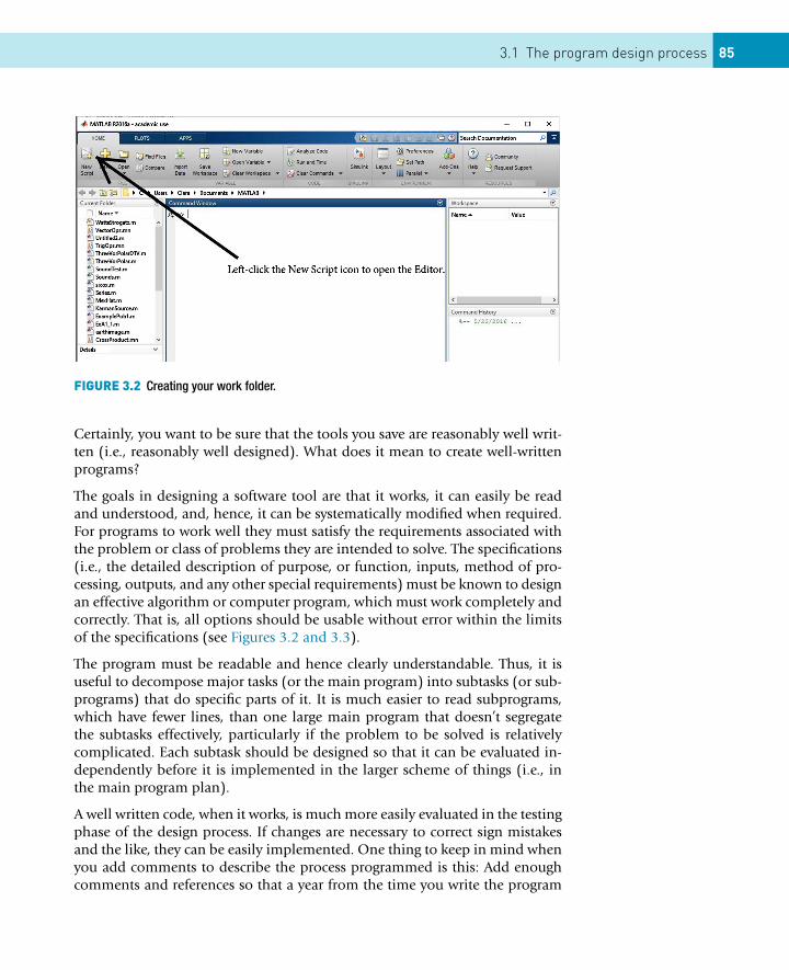
3.1 The program design process 85
FIGURE 3.2 Creating your work folder.
Certainly, you want to be sure that the tools you save are reasonably well writ-ten (i.e., reasonably well designed). What does it mean to create well-writtenprograms?
The goals in designing a software tool are that it works, it can easily be readand understood, and, hence, it can be systematically modified when required.For programs to work well they must satisfy the requirements associated withthe problem or class of problems they are intended to solve. The specifications(i.e., the detailed description of purpose, or function, inputs, method of pro-cessing, outputs, and any other special requirements) must be known to designan effective algorithm or computer program, which must work completely andcorrectly. That is, all options should be usable without error within the limitsof the specifications (see Figures 3.2 and 3.3).
The program must be readable and hence clearly understandable. Thus, it isuseful to decompose major tasks (or the main program) into subtasks (or sub-programs) that do specific parts of it. It is much easier to read subprograms,which have fewer lines, than one large main program that doesn’t segregatethe subtasks effectively, particularly if the problem to be solved is relativelycomplicated. Each subtask should be designed so that it can be evaluated in-dependently before it is implemented in the larger scheme of things (i.e., inthe main program plan).
A well written code, when it works, is much more easily evaluated in the testingphase of the design process. If changes are necessary to correct sign mistakesand the like, they can be easily implemented. One thing to keep in mind whenyou add comments to describe the process programmed is this: Add enoughcomments and references so that a year from the time you write the program
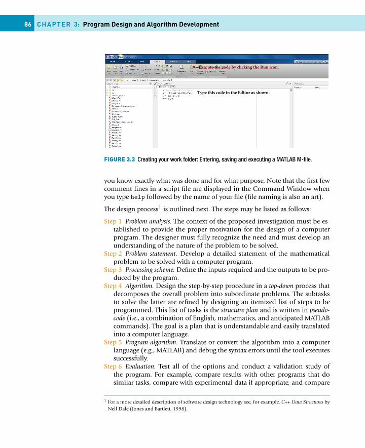
86 CHAPTER 3: Program Design and Algorithm Development
FIGURE 3.3 Creating your work folder: Entering, saving and executing a MATLAB M-file.
you know exactly what was done and for what purpose. Note that the first fewcomment lines in a script file are displayed in the Command Window whenyou type help followed by the name of your file (file naming is also an art).
The design process1 is outlined next. The steps may be listed as follows:
Step 1 Problem analysis. The context of the proposed investigation must be es-tablished to provide the proper motivation for the design of a computerprogram. The designer must fully recognize the need and must develop anunderstanding of the nature of the problem to be solved.
Step 2 Problem statement. Develop a detailed statement of the mathematicalproblem to be solved with a computer program.
Step 3 Processing scheme. Define the inputs required and the outputs to be pro-duced by the program.
Step 4 Algorithm. Design the step-by-step procedure in a top-down process thatdecomposes the overall problem into subordinate problems. The subtasksto solve the latter are refined by designing an itemized list of steps to beprogrammed. This list of tasks is the structure plan and is written in pseudo-code (i.e., a combination of English, mathematics, and anticipated MATLABcommands). The goal is a plan that is understandable and easily translatedinto a computer language.
Step 5 Program algorithm. Translate or convert the algorithm into a computerlanguage (e.g., MATLAB) and debug the syntax errors until the tool executessuccessfully.
Step 6 Evaluation. Test all of the options and conduct a validation study ofthe program. For example, compare results with other programs that dosimilar tasks, compare with experimental data if appropriate, and compare
1 For a more detailed description of software design technology see, for example, C++ Data Structures byNell Dale (Jones and Bartlett, 1998).
3.1 The program design process 87
with theoretical predictions based on theoretical methodology related tothe problems to be solved. The objective is to determine that the subtasksand the overall program are correct and accurate. The additional debuggingin this step is to find and correct logical errors (e.g., mistyping of expressionsby putting a plus sign where a minus sign was supposed to be) and runtimeerrors that may occur after the program successfully executes (e.g., caseswhere division by zero unintentially occurs).
Step 7 Application. Solve the problems the program was designed to solve. Ifthe program is well designed and useful, it can be saved in your workingdirectory (i.e., in your user-developed toolbox) for future use.
3.1.1 The projectile problemStep 1. Let us consider the projectile problem examined in first-semesterphysics. It is assumed that engineering and science students understand thisproblem (if it is not familiar to you, find a physics text that describes it orsearch the Web; the formulas that apply will be provided in step 2).
In this example we want to calculate the flight of a projectile (e.g., a golfball) launched at a prescribed speed and a prescribed launch angle. We wantto determine the trajectory of the flight path and the horizontal distance theprojectile (or object) travels before it hits the ground. Let us assume zero airresistance and a constant gravitational force acting on the object in the oppo-site direction of the vertical distance from the ground. The launch angle, θo,is defined as the angle measured from the horizontal (ground plane) upwardtoward the vertical direction, 0 < θo ≤ π/2, where θo = 0 implies a launch inthe horizontal direction and θo = π/2 implies a launch in the vertical direction(i.e., in the opposite direction of gravity). If g = 9.81 m/s2 is used as the accel-eration of gravity, the launch speed, Vo, must be entered in units of m/s. Thus,if the time, t > 0, is the time in seconds (s) from the launch time of t = 0, thedistance traveled in x (the horizontal direction) and y (the vertical direction)is in meters (m).
We want to determine the time it takes the projectile, from the start of motion,to hit the ground, the horizontal distance traveled, and the shape of the trajec-tory. In addition, we want to plot the speed of the projectile versus the angulardirection of this vector. We need, of course, the theory (or mathematical ex-pressions) that describes the solution to the zero-resistance projectile problemin order to develop an algorithm to obtain solutions to it.
Step 2. The mathematical formulas that describe the solution to the projectileproblem are provided in this step. Given the launch angle and launch speed,the horizontal distance traveled from x = y = 0, which is the coordinate loca-tion of the launcher, is
xmax = 2V 2
o
gsin θo cos θo
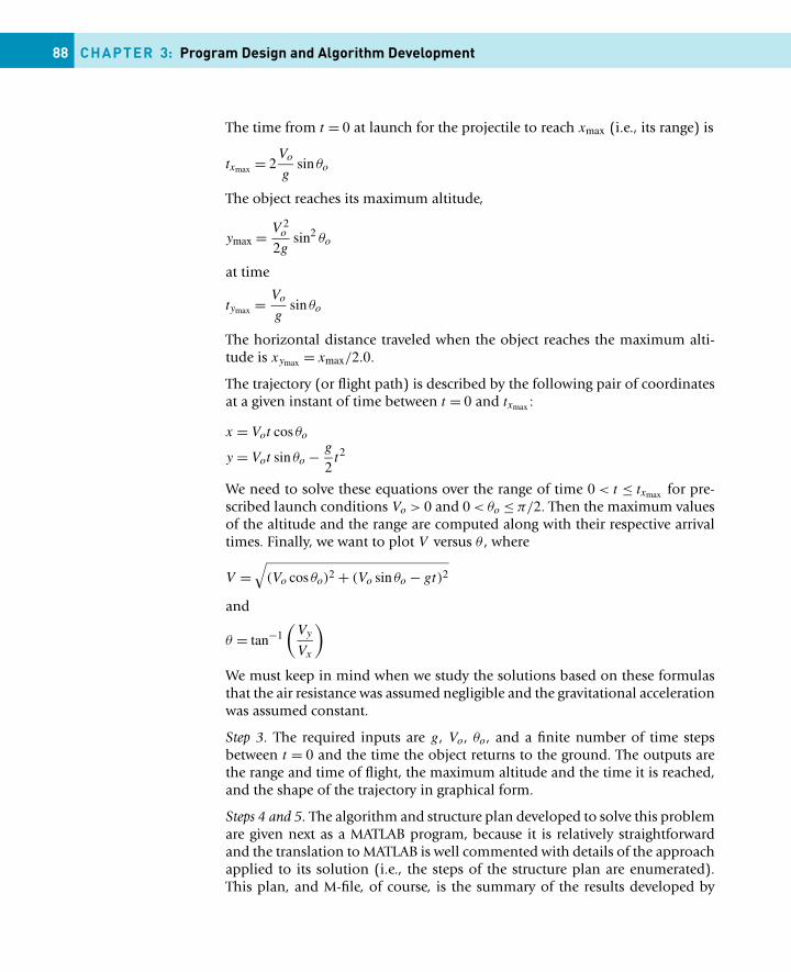
88 CHAPTER 3: Program Design and Algorithm Development
The time from t = 0 at launch for the projectile to reach xmax (i.e., its range) is
txmax = 2Vo
gsin θo
The object reaches its maximum altitude,
ymax = V 2o
2gsin2 θo
at time
tymax = Vo
gsin θo
The horizontal distance traveled when the object reaches the maximum alti-tude is xymax = xmax/2.0.
The trajectory (or flight path) is described by the following pair of coordinatesat a given instant of time between t = 0 and txmax :
x = Vot cos θo
y = Vot sin θo − g
2t2
We need to solve these equations over the range of time 0 < t ≤ txmax for pre-scribed launch conditions Vo > 0 and 0 < θo ≤ π/2. Then the maximum valuesof the altitude and the range are computed along with their respective arrivaltimes. Finally, we want to plot V versus θ , where
V =√
(Vo cos θo)2 + (Vo sin θo − gt)2
and
θ = tan−1(
Vy
Vx
)
We must keep in mind when we study the solutions based on these formulasthat the air resistance was assumed negligible and the gravitational accelerationwas assumed constant.
Step 3. The required inputs are g, Vo, θo, and a finite number of time stepsbetween t = 0 and the time the object returns to the ground. The outputs arethe range and time of flight, the maximum altitude and the time it is reached,and the shape of the trajectory in graphical form.
Steps 4 and 5. The algorithm and structure plan developed to solve this problemare given next as a MATLAB program, because it is relatively straightforwardand the translation to MATLAB is well commented with details of the approachapplied to its solution (i.e., the steps of the structure plan are enumerated).This plan, and M-file, of course, is the summary of the results developed by
3.1 The program design process 89
trying a number of approaches during the design process, and thus discard-ing numerous sheets of scratch paper before summarizing the results! (Thereare more explicit examples of structure plans for your review and investigationin the next section of this chapter.) Keep in mind that it was not difficult toenumerate a list of steps associated with the general design process, that is,the technical problem solving. However, it is certainly not so easy to imple-ment the steps because they draw heavily on your technical-solution designexperience. Hence, we must begin by studying the design of relatively simpleprograms like the one described in this section.
The evaluated and tested code is as follows:
% The proctile problem with zero air resistance% in a gravitational field with constant g.% Written by Daniel T. Valentine .. September 2006% Revised by D. T. Valentine ........... 2012/2016% An eight-step structure plan applied in MATLAB:%% 1. Define the input variables.%g = 9.81; % Gravity in m/s/s.vo = input(’What is the launch speed in m/s? ’)tho = input(’What is the launch angle in degrees? ’)tho = pi*tho/180; % Conversion of degrees to radians.%% 2. Calculate the range and duration of the flight.%txmax = (2*vo/g) * sin(tho);xmax = txmax * vo * cos(tho);%% 3. Calculate the sequence of time steps to compute% trajectory.%dt = txmax/100;t = 0:dt:txmax;%% 4. Compute the trajectory.%x = (vo * cos(tho)) .* t;y = (vo * sin(tho)) .* t - (g/2) .* t.^2;%% 5. Compute the speed and angular direction of the% projectile. Note that vx = dx/dt, vy = dy/dt.%vx = vo * cos(tho);
90 CHAPTER 3: Program Design and Algorithm Development
vy = vo * sin(tho) - g .* t;v = sqrt(vx.*vx + vy.*vy); % Speedth = (180/pi) .* atan2(vy,vx); % Angular direction%% 6. Compute the time and horizontal distance at the% maximum altitude.%tymax = (vo/g) * sin(tho);xymax = xmax/2;ymax = (vo/2) * tymax * sin(tho);%% 7. Display in the Command Window and on figures the ouput.%disp([’Range in meters = ’,num2str(xmax),’,’ ...
’ Duration in seconds = ’, num2str(txmax)])disp(’ ’)disp([’Maximum altitude in meters = ’,num2str(ymax), ...
’, Arrival at this altitude in seconds = ’, num2str(tymax)])plot(x,y,’k’,xmax,y(size(t)),’o’,xmax/2,ymax,’o’)title([’Projectile flight path: v_o = ’, num2str(vo),’ m/s’ ...
’, \theta_o = ’, num2str(180*tho/pi),’ degrees’])xlabel(’x’), ylabel(’y’) % Plot of Figure 3.4.figure % Creates a new figure.plot(v,th,’r’)title(’Projectile speed vs. angle’)xlabel(’V’), ylabel(’\theta’) % Plot of Figure 3.5.%% 8. Stop.
Steps 6 and 7. The program was evaluated by executing a number of values ofthe launch angle and launch speed within the required specifications. The an-gle of 45 degrees was checked to determine that the maximum range occurredat this angle for all specified launch speeds. This is well known for the zero airresistance case in a constant g force field. Executing this code for Vo = 10 m/sand θo = 45 degrees, the trajectory and the plot of orientation versus speed inFigures 3.4 and 3.5, respectively, were produced.
How can you find additional examples of MATLAB programs (good ones orotherwise) to help develop tools to solve your own problems? We all recog-nize that examples aren’t a bad way of learning to use tools. New tools arecontinually being developed by the users of MATLAB. If one proves to be ofmore general use, MathWorks may include it in their list of products (if, ofcourse, the tools’ author desires this). There are also many examples of use-ful scripts that are placed on the Web for anyone interested in them. They, ofcourse, must be evaluated carefully since it is the user’s responsibility, not the
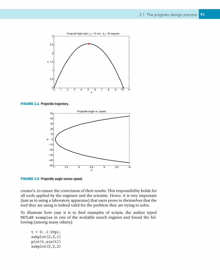
3.1 The program design process 91
FIGURE 3.4 Projectile trajectory.
FIGURE 3.5 Projectile angle versus speed.
creator’s, to ensure the correctness of their results. This responsibility holds forall tools applied by the engineer and the scientist. Hence, it is very important(just as in using a laboratory apparatus) that users prove to themselves that thetool they are using is indeed valid for the problem they are trying to solve.
To illustrate how easy it is to find examples of scripts, the author typedMATLAB examples in one of the available search engines and found the fol-lowing (among many others):
t = 0:.1:2*pi;subplot(2,2,1)plot(t,sin(t))subplot(2,2,2)
92 CHAPTER 3: Program Design and Algorithm Development
plot(t,cos(t))subplot(2,2,3)plot(t,exp(t))subplot(2,2,4)plot(t,1./(1+t.^2))
This script illustrates how to put four plots in a single figure window. To checkthat it works, type each line in the Command Window followed by Enter. Notethe position of each graphic; location is determined by the three integers in thesubplot function list of arguments. Search Help via the question mark (?) formore information on subplot.
3.2 PROGRAMMING MATLAB FUNCTIONS
MATLAB enables you to create your own function M-files. A function M-file issimilar to a script file in that it also has a .m extension. However, a functionM-file differs from a script file in that a function M-file communicates with theMATLAB workspace only through specially designated input and output argu-ments. Functions are indispensable tools when it comes to breaking a problemdown into manageable logical pieces.
Short mathematical functions may be written as one-line inline objects. Thiscapability is illustrated by example in the next subsection. In the subsequentsubsection essential ideas embodied in the creation of a MATLAB functionM-file will be introduced. (Further details on writing functions are provided inChapter 4.)
3.2.1 Inline objects: Harmonic oscillatorsIf two coupled harmonic oscillators, e.g., two masses connected with a springon a very smooth table, are considered as a single system, the output of thesystem as a function of time t could be given by something like
h(t) = cos(8t) + cos(9t). (3.1)
You can represent h(t) at the command line by creating an inline object as fol-lows:
h = inline( ’cos(8*t) + cos(9*t)’ );
Now write some MATLAB statements in the Command Window which useyour function h to draw the graph in Figure 3.6 e.g.,
x = 0 : 20/300 : 20;plot(x, h(x)), grid
Note:
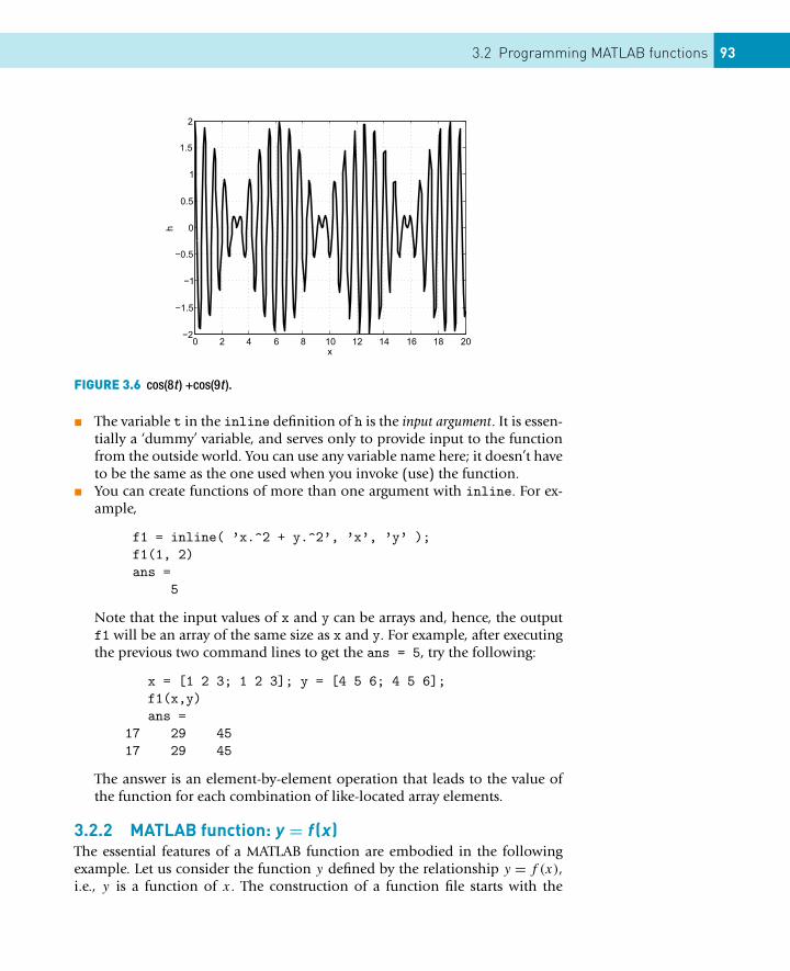
3.2 Programming MATLAB functions 93
FIGURE 3.6 cos(8t ) +cos(9t ).
� The variable t in the inline definition of h is the input argument. It is essen-tially a ‘dummy’ variable, and serves only to provide input to the functionfrom the outside world. You can use any variable name here; it doesn’t haveto be the same as the one used when you invoke (use) the function.
� You can create functions of more than one argument with inline. For ex-ample,
f1 = inline( ’x.^2 + y.^2’, ’x’, ’y’ );f1(1, 2)ans =
5
Note that the input values of x and y can be arrays and, hence, the outputf1 will be an array of the same size as x and y. For example, after executingthe previous two command lines to get the ans = 5, try the following:
x = [1 2 3; 1 2 3]; y = [4 5 6; 4 5 6];f1(x,y)ans =
17 29 4517 29 45
The answer is an element-by-element operation that leads to the value ofthe function for each combination of like-located array elements.
3.2.2 MATLAB function: y = f (x)The essential features of a MATLAB function are embodied in the followingexample. Let us consider the function y defined by the relationship y = f (x),i.e., y is a function of x. The construction of a function file starts with the
94 CHAPTER 3: Program Design and Algorithm Development
declaration of a function command. This is followed by the formula that is thefunction of interest that you wish to substitute a particular value of x to get thecorresponding value of y. The structure plan for the evaluation of a particularalgebraic function is as follows:
1. function y = f(x) % where $x$ is the input and $y$ is theoutput.
2. y = x.^3 - 0.95*x;3. end % This is not necessary to include; however, it plays the
role of STOP.
The function M-file created based on this plan is as follows:
function y = f(x)% where $x$ is the input and $y$ is the output.|
y = x.^3 - 0.95*x;end % This is not necessary to include; however, it plays the
role of STOP.
It was saved as f.m. After saving it, it was used as follows in the CommandWindow. Try the following example:
>> f(2)ans =
6.1000
Let us next create a function that takes as input the three coefficients of thequadratic equation, viz.,
ax2 + bx + c = 0.
We want the determine the two roots of this equation, i.e., we want to deter-mine the solution to this equation. One way of dealing with this problem is toapply the known solutions of the quadratic equation. Let us do this by creatinga function file by following the structure plan for the complete algorithm forfinding the solution(s) x, given the coefficients a, b and c given as follows:
QUADRATIC EQUATION STRUCTURE PLAN
1. Start2. Input data (a, b, c)3. If a = 0 then
If b = 0 thenIf c = 0 then
Display ‘Solution indeterminate’
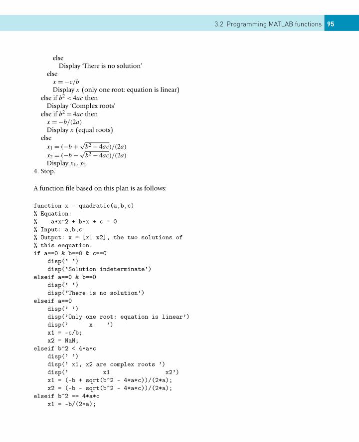
3.2 Programming MATLAB functions 95
elseDisplay ‘There is no solution’
elsex = −c/b
Display x (only one root: equation is linear)else if b2 < 4ac then
Display ‘Complex roots’else if b2 = 4ac then
x = −b/(2a)
Display x (equal roots)else
x1 = (−b + √b2 − 4ac)/(2a)
x2 = (−b − √b2 − 4ac)/(2a)
Display x1, x24. Stop.
A function file based on this plan is as follows:
function x = quadratic(a,b,c)% Equation:% a*x^2 + b*x + c = 0% Input: a,b,c% Output: x = [x1 x2], the two solutions of% this eequation.if a==0 & b==0 & c==0
disp(’ ’)disp(’Solution indeterminate’)
elseif a==0 & b==0disp(’ ’)disp(’There is no solution’)
elseif a==0disp(’ ’)disp(’Only one root: equation is linear’)disp(’ x ’)x1 = -c/b;x2 = NaN;
elseif b^2 < 4*a*cdisp(’ ’)disp(’ x1, x2 are complex roots ’)disp(’ x1 x2’)x1 = (-b + sqrt(b^2 - 4*a*c))/(2*a);x2 = (-b - sqrt(b^2 - 4*a*c))/(2*a);
elseif b^2 == 4*a*cx1 = -b/(2*a);
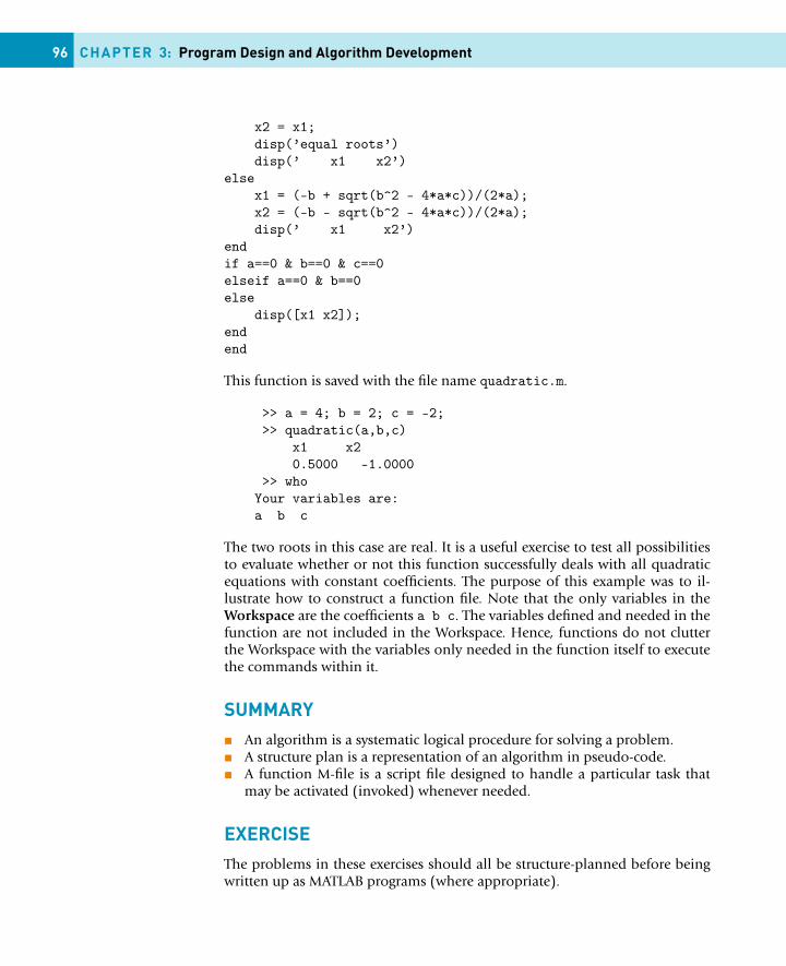
96 CHAPTER 3: Program Design and Algorithm Development
x2 = x1;disp(’equal roots’)disp(’ x1 x2’)
elsex1 = (-b + sqrt(b^2 - 4*a*c))/(2*a);x2 = (-b - sqrt(b^2 - 4*a*c))/(2*a);disp(’ x1 x2’)
endif a==0 & b==0 & c==0elseif a==0 & b==0else
disp([x1 x2]);endend
This function is saved with the file name quadratic.m.
>> a = 4; b = 2; c = -2;>> quadratic(a,b,c)
x1 x20.5000 -1.0000
>> whoYour variables are:a b c
The two roots in this case are real. It is a useful exercise to test all possibilitiesto evaluate whether or not this function successfully deals with all quadraticequations with constant coefficients. The purpose of this example was to il-lustrate how to construct a function file. Note that the only variables in theWorkspace are the coefficients a b c. The variables defined and needed in thefunction are not included in the Workspace. Hence, functions do not clutterthe Workspace with the variables only needed in the function itself to executethe commands within it.
SUMMARY� An algorithm is a systematic logical procedure for solving a problem.� A structure plan is a representation of an algorithm in pseudo-code.� A function M-file is a script file designed to handle a particular task that
may be activated (invoked) whenever needed.
EXERCISEThe problems in these exercises should all be structure-planned before beingwritten up as MATLAB programs (where appropriate).
3.2 Exercise 97
3.1 The structure plan in this example defines a geometric construction. Carryout the plan by sketching the construction:1. Draw two perpendicular x- and y-axes2. Draw the points A (10, 0) and B (0, 1)3. While A does not coincide with the origin repeat: Draw a straight line
joining A and B Move A one unit to the left along the x-axis MoveB one unit up on the y-axis
4. Stop3.2 Consider the following structure plan, where M and N represent MATLAB
variables:1. Set M = 44 and N = 282. While M not equal to N repeat: While M > N repeat: Replace value
of M by M − N While N > M repeat: Replace value of N by N − M
3. Display M
4. Stop(a) Work through the structure plan, sketching the contents of M and
N during execution. Give the output.(b) Repeat (a) for M = 14 and N = 24.(c) What general arithmetic procedure does the algorithm carry out
(try more values of M and N if necessary)?3.3 Write a program to convert a Fahrenheit temperature to Celsius. Test it on
the data in Exercise 2.11 (where the reverse conversion is done).3.4 Write a script that inputs any two numbers (which may be equal) and
displays the larger one with a suitable message or, if they are equal, displaysa message to that effect.
3.5 Write a script for the general solution to the quadratic equation ax2 +bx +c = 0. Use the structure plan in Section 3.2.2. Your script should be able tohandle all possible values of the data a, b, and c. Try it out on the followingvalues:(a) 1, 1, 1 (complex roots)(b) 2, 4, 2 (equal roots of −1.0)(c) 2, 2, −12 (roots of 2.0 and −3.0)The structure plan in Section 3.2.2 is for programming languages that can-not handle complex numbers. MATLAB can. Adjust your script so that itcan also find complex roots. Test it on case (a); the roots are −0.5 ± 0.866i.
3.6 Develop a structure plan for the solution to two simultaneous linear equa-tions (i.e., the equations of two straight lines). Your algorithm must beable to handle all possible situations; that is, lines intersecting, parallel, orcoincident. Write a program to implement your algorithm, and test it onsome equations for which you know the solutions, such as
x + y = 3
2x − y = 3
(x = 2, y = 1).
98 CHAPTER 3: Program Design and Algorithm Development
Hint: Begin by deriving an algebraic formula for the solution to the system:
ax + by = c
dx + ey = f
The program should input the coefficients a, b, c, d , e, and f .We will see in Chapter 6 that MATLAB has a very elegant way of solvingsystems of equations directly, using matrix algebra. However, it is good forthe development of your programming skills to do it the long way, as inthis exercise.
3.7 We wish to examine the motion of a damped harmonic oscillator. Thesmall amplitude oscillation of a unit mass attached to a spring is given bythe formula y = e−(R/2)t sin(ω1t), where ω2
1 = ω2o − R2/4 is the square of
the natural frequency of the oscillation with damping (i.e., with resistanceto motion); ω2
o = k is the square of the natural frequency of undampedoscillation; k is the spring constant; and R is the damping coefficient. Con-sider k = 1 and vary R from 0 to 2 in increments of 0.5. Plot y versus t fort from 0 to 10 in increments of 0.1.Hint: Develop a solution procedure by working backwards through theproblem statement. Starting at the end of the problem statement, the solu-tion procedure requires the programmer to assign the input variables firstfollowed by the execution of the formula for the amplitude and endingwith the output in graphical form.
3.8 Let’s examine the shape of a uniform cable hanging under its own weight.The shape is described by the formula y = cosh(x/c). This shape is calleda uniform catenary. The parameter c is the vertical distance from y = 0where the bottom of the catenary is located. Plot the shape of the catenarybetween x = −10 and x = 10 for c = 5. Compare this with the same resultfor c = 4.Hint: The hyperbolic cosine, cosh, is a built-in MATLAB function that isused in a similar way to the sine function, sin.
CONTENTS
Commonfunctions ............... 99
Importing andexporting data ... 104The load and savecommands............. 104Exporting text (ASCII)data ....................... 104Importing text (ASCII)data ....................... 105Exporting binarydata ....................... 105Importing binarydata ....................... 106
Summary ............ 106
Exercises ............ 106
CHAPTER 4
MATLAB Functions and DataImport-Export Utilities
THE OBJECTIVES OF THIS CHAPTER ARE:
(1) To enable you to become familiar with some of the more commonMATLAB functions.
(2) To introduce you briefly to ways of importing and exporting data in andout of the MATLAB workspace using:� The load and save commands.� The Import Wizard.� The low-level file input/output (I/O) functions.
At this point you should be able to write a MATLAB program which inputsdata, performs simple arithmetic operations on the data, perhaps involvingloops and decisions, and displays the results of the computation in a compre-hensible form. However, more interesting problems in science and engineeringare likely to involve special mathematical functions like sines, cosines, loga-rithms, etc. MATLAB comes with a large collection of such functions; we haveseen some of them already. This chapter introduces you to the more commonfunctions available in MATLAB. In addition, you may wish to import data to beplotted or operated on mathematically, and export data for future use. Hence,this chapter also introduces you to the importing of data into the MATLABworkspace from various sources. It also discusses the exporting of data to filesin your work directory for later use with MATLAB or with other software tools.
4.1 COMMON FUNCTIONS
Tables of MATLAB functions and commands appear in Appendix C. A short listof some of the more common ones follows. Use helpwin at the command lineto see a list of categories of functions, with links to descriptions of the func-tions. Alternatively, go to the Contents listing in the Help Navigator (the leftpane in the Help browser), and expand successively MATLAB, Reference, MAT-
99Essential MATLAB for Engineers and Scientists. DOI:10.1016/B978-0-08-100877-5.00005-0Copyright © 2017 Daniel T. Valentine. Published by Elsevier Ltd. All rights reserved.
100 CHAPTER 4: MATLAB Functions
LAB Function Reference where you can choose either Functions by Category,or Alphabetical List of Functions.
Note that if the argument of a function is an array, the function is appliedelement by element to all the values in the array, e.g.,
sqrt([1 2 3 4])
returns
1.0000 1.4142 1.7321 2.0000
Since this text is written in a tutorial style, it is expected that you will examinethe following list of some of the more common functions in MATLAB. It isalso, to some extent, expected that you already know, from your first courses inmathematics and science, something about these functions. One way to exam-ine these functions is to plot them. Have some fun experimenting with MAT-LAB in your investigation of the following functions! For example, do the fol-lowing exercise for all functions of the assigned variable x, as illustrated next.
x = -1:.1:1; <Enter>plot(x,abs(x),’o’) <Enter>
You should get an illustration that looks like a V.
abs(x)absolute value of x.
acos(x)arc cosine (inverse cosine) of x between 0 and π .
acosh(x)inverse hyperbolic cosine of x, i.e., ln(x + √
x2 − 1).asin(x)
arc sine (inverse sine) of x between −π/2 and π/2.asinh(x)
inverse hyperbolic sine of x, i.e., ln(x + √x2 + 1).
atan(x)arc tangent of x between −π/2 and π/2.
atan2(y, x)arc tangent of y/x between −π and π .
atanh(x)
inverse hyperbolic tangent of x, i.e.,1
2ln
(1 + x
1 − x
).
ceil(x)smallest integer which exceeds x, i.e., rounds up to nearest integer, e.g.,ceil(-3.9) returns -3, ceil(3.9) returns 4.
4.1 Common functions 101
FIGURE 4.1 (a) Exponential, (b) hyperbolic sine and (c) hyperbolic cosine functions.
clocktime and date in a six-element vector, e.g., the statements
t = clock;fprintf( ’ %02.0f:%02.0f:%02.0f\n’, t(4), t(5), t(6) );
result in 14:09:03. Note how the hours, minutes and seconds are left-filledwith zeros if necessary.
cos(x)cosine of x.
cosh(x)
hyperbolic cosine of x, i.e.,ex + e−x
2(see Figure 4.1).
cot(x)cotangent of x.
csc(x)cosecant of x.
cumsum(x)cumulative sum of the elements of x, e.g., cumsum(1:4) returns [1 3 6 10].
datedate in a string in dd-mmm-yyyy format, e.g., 02-Feb-2001.
exp(x)value of the exponential function ex (see Figure 4.1).
fix(x)rounds to the nearest integer towards zero, e.g., fix(-3.9) returns -3,fix(3.9) returns 3.
floor(x)largest integer not exceeding x, i.e., rounds down to nearest integer, e.g.,floor(-3.9) returns -4, floor(3.9) returns 3.
102 CHAPTER 4: MATLAB Functions
length(x)number of elements of vector x.
log(x)natural logarithm of x.
log10(x)base 10 logarithm of x.
max(x)maximum element of vector x.
mean(x)mean value of elements of vector x.
min(x)minimum element of vector x.
pow2(x)2x .
prod(x)product of the elements of x.
randpseudo-random number in the interval (0, 1). The value returned is pseudo-random rather than truly random in the sense that there is an algorithm thatdetermines rand from the initial ‘seed’. The same seed will generate the same‘random’ sequence; see a later chapter for how to seed rand by looking inthe index.
realmaxlargest positive floating point number on your computer.
realminsmallest positive floating point number on your computer.
rem(x, y)remainder when x is divided by y, e.g., rem(19, 5) returns 4 (5 goes 3 times
into 19, remainder 4).Strictly, rem(x, y) returns x - y * n where n = fix(x/y) is the integernearest to x/y. This shows how negative and/or non-integer arguments arehandled.fix and rem are useful for converting smaller units to larger ones, e.g., inchesto feet and inches (one foot = 12 inches). The following statements convert40 inches this way:
feet = fix(40/12)inches = rem(40, 12)
Let us next examine an example that will hopefully inspire you to examine allof the functions listed as well as any other function that you may discoverthat MATLAB supports. Let us consider the arc-cosine, the arc-sine and thearc-tangent functions, i.e., acos(x), asin(x) and atan(x), respectively. If youspecify x, i.e., the cosine, the sine and the tangent, respectively, between −1and 1, what quadrant of the circle are the output angles selected? To provide
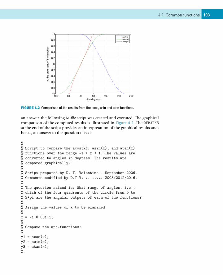
4.1 Common functions 103
FIGURE 4.2 Comparison of the results from the acos, asin and atan functions.
an answer, the following M-file script was created and executed. The graphicalcomparison of the computed results is illustrated in Figure 4.2. The REMARKSat the end of the script provides an interpretation of the graphical results and,hence, an answer to the question raised.
%% Script to compare the acos(x), asin(x), and atan(x)% functions over the range -1 < x < 1. The values are% converted to angles in degrees. The results are% compared graphically.%% Script prepared by D. T. Valentine - September 2006.% Comments modified by D.T.V. ........ 2008/2012/2016.%% The question raised is: What range of angles, i.e.,% which of the four quadrents of the circle from 0 to% 2*pi are the angular outputs of each of the functions?%% Assign the values of x to be examined:%x = -1:0.001:1;%% Compute the arc-functions:%y1 = acos(x);y2 = asin(x);y3 = atan(x);%
104 CHAPTER 4: MATLAB Functions
% Convert the angles from radians to degrees:%y1 = 180*y1/pi;y2 = 180*y2/pi;y3 = 180*y3/pi;%% Plot the results:%plot(y1,x,y2,x,y3,x),gridlegend(’asin(x)’, ’acos(x)’, ’atan(x)’)xlabel(’\theta in degrees’)ylabel(’x, the argument of the function’)%% REMARKS: Note the following:% (1) The acos(x) varies from 0 to 90 to 180 degrees.% (2) The asin(x) varies from -90 to 0 to 90 degrees.% (3) The atan(x) varies from -90 to 0 to 90 degrees.% To check remark (3) try atan(10000000) *180/pi.%% Stop
4.2 IMPORTING AND EXPORTING DATA
When you get into serious programming you will often need to store data ona disk. The process of moving data between MATLAB and disk files is calledimporting (from disk files) and exporting (to disk files). Data are saved in diskfiles in one of two formats: text or binary. In text format, data values are ASCIIcodes, and can be viewed in any text editor. In binary format, data values arenot ASCII codes and cannot be viewed in a text editor. Binary format is moreefficient in terms of storage space required. This chapter provides a brief sum-mary of the main ways in which MATLAB imports and exports data. For fulldetails consult MATLAB Help: Development Environment: Importing andExporting Data.
4.2.1 The load and save commandsIf you want to save data between MATLAB sessions the save and load com-mands are probably the best ones to use.
4.2.2 Exporting text (ASCII) dataTo export (save) the array
A =1 2 34 5 6
4.2 Importing and exporting data 105
in ‘delimited’ ASCII format in the file myData.txt use the command
save myData.txt A -ascii
If you view myData.txt in a text editor (or type it in the Command Window)it looks like this:
1.0000000e+000 2.0000000e+000 3.0000000e+0004.0000000e+000 5.0000000e+000 6.0000000e+000
Delimiters are the characters used to separate the data values in the file—spacesby default. You can use tabs instead of spaces by specifying the -tabs qualifierinstead of -ascii. If you save character arrays (strings) in this way, the ASCIIcodes of the characters are written to the file.
4.2.3 Importing text (ASCII) dataThe load command is the reverse of save, but has a curious twist. If the arrayA has been saved in myData.txt as above the command
load myData.txt
creates a variable in the workspace with the same name as the file, minus theextension, i.e., myData. If you don’t want the filename as the variable name usethe functional form of the command, e.g.,
A = load(’myData.txt’)
Data imported in this way doesn’t have to be created by MATLAB. You cancreate it in a text editor, or it could be created by any other program that exportsdata in ASCII format.
4.2.4 Exporting binary dataThe command
save filename x y z
saves the variables x, y and z in the file filename.mat in MATLAB proprietarybinary format, i.e., such a MAT-file can only be used by MATLAB.
106 CHAPTER 4: MATLAB Functions
Note:
� If no variables are listed the entire workspace is saved.� The extension .mat is the default—you can specify a different extension.� Seek help for all the save options.
4.2.5 Importing binary dataThe command
load filename
loads all the variables from filename.mat into the workspace; see help for allthe load options.
SUMMARY� MATLAB functions may be used to perform a variety of mathematical,
trigonometric and other operations.� Data can be saved to disk files in text (ASCII) format or in binary format.� load and save can be used to import/export both text and binary data (the
latter in the form of MAT-files).
EXERCISES4.1 Write some MATLAB statements which will:
(a) find the length C of the hypotenuse of a right-angle triangle in termsof the lengths A and B of the other two sides;
(b) find the length C of a side of a triangle given the lengths A and B ofthe other two sides and the size in degrees of the included angle θ ,using the cosine rule:
C2 = A2 + B2 − 2AB cos(θ).
4.2 Translate the following formulae into MATLAB expressions:(a) ln(x + x2 + a2)
(b) [e3t + t2 sin(4t)] cos2(3t)
(c) 4 tan−1(1) (inverse tangent)(d) sec2(x) + cot(y)
(e) cot−1(|x/a|) (use MATLAB’s inverse cotangent)4.3 There are 39.37 inches in a meter, 12 inches in a foot, and three feet in a
yard. Write a script to input a length in meters (which may have a decimalpart) and convert it to yards, feet and inches. (Check: 3.51 meters convertsto 3 yds 2 ft 6.19 in.)
4.4 A sphere of mass m1 impinges obliquely on a stationary sphere of mass m2,the direction of the blow making an angle α with the line of motion of the
4.2 Exercises 107
impinging sphere. If the coefficient of restitution is e it can be shown thatthe impinging sphere is deflected through an angle β such that
tan(β) = m2(1 + e) tan(α)
m1 − em2 + (m1 + m2) tan2(α)
Write a script to input values of m1, m2, e, and α (in degrees) and to com-pute the angle β in degrees.
4.5 Section 2.7 has a program for computing the members of the sequencexn = an/n!. The program displays every member xn computed. Adjust it todisplay only every 10th value of xn.Hint: the expression rem(n, 10) will be zero only when n is an exact mul-tiple of 10.Use this in an if statement to display every tenth value of xn.
4.6 To convert the variable mins minutes into hours and minutes you woulduse fix(mins/60) to find the whole number of hours, and rem(mins,60) to find the number of minutes left over. Write a script which inputs anumber of minutes and converts it to hours and minutes.Now write a script to convert seconds into hours, minutes and seconds.Try out your script on 10 000 seconds, which should convert to 2 hours 46minutes and 40 seconds.
4.7 Design an algorithm (i.e., write the structure plan) for a machine whichmust give the correct amount of change from a $100 note for any purchasecosting less than $100. The plan must specify the number and type of allnotes and coins in the change, and should in all cases give as few notesand coins as possible. (If you are not familiar with dollars and cents, useyour own monetary system.)
4.8 A uniform beam is freely hinged at its ends x = 0 and x = L, so that theends are at the same level. It carries a uniformly distributed load of W perunit length, and there is a tension T along the x-axis. The deflection y ofthe beam a distance x from one end is given by
y = WEI
T 2
[cosh[a(L/2 − x)]
cosh(aL/2)− 1
]+ Wx(L − x)
2T,
where a2 = T/EI , E being the Young’s modulus of the beam, and I is themoment of inertia of a cross-section of the beam. The beam is 10 m long,the tension is 1 000 N, the load 100 N/m, and EI is 104.Write a script to compute and plot a graph of the deflection y against x
(MATLAB has a cosh function).To make the graph look realistic you will have to override MATLAB’s auto-matic axis scaling with the statement
axis( [xmin xmax ymin ymax] )
after the plot statement, where xmin etc. have appropriate values.
CONTENTS
Examples ............. 110Discontinuousgraphs .................... 110Avoiding division byzero......................... 111Avoiding infinity ......112Counting randomnumbers .................113Rolling dice.............114
Logicaloperators .............114Operatorprecedence .............116Danger....................116Logical operators andvectors....................117
Subscripting withlogical vectors ....118
Logicalfunctions ..............119Using any and all.. 120
Logical vectorsinstead of elseifladders ................ 121
Summary ............ 123
Exercises ............ 124
CHAPTER 5
Logical Vectors
THE OBJECTIVES OF THIS CHAPTER ARE TO ENABLE YOUTO:
� Understand logical operators more fully
And to introduce you to:
� Logical vectors and how to use them effectively in a number ofapplications
� Logical functions
This chapter introduces a most powerful and elegant feature of MATLAB, viz.,the logical vectors. The topic is so useful and, hence, important that it deservesa chapter of its own.
Try these exercises on the command line:
1. Enter the following statements:
r = 1;r <= 0.5 % no semi-colon
If you correctly left out the semi-colon after the second statement you willhave noticed that it returned the value 0.
2. Now enter the expression r >= 0.5 (again, no semi-colon). It should re-turn the value 1. Note that we already saw in Chapter 2 that a logicalexpression in MATLAB involving only scalars returns a value of 0 if it isFALSE, and 1 if it is TRUE.
3. Enter the following statements:
r = 1:5;r <= 3
Now the logical expression r <= 3 (where r is a vector) returns a vector:109
Essential MATLAB for Engineers and Scientists. DOI:10.1016/B978-0-08-100877-5.00006-2Copyright © 2017 Daniel T. Valentine. Published by Elsevier Ltd. All rights reserved.
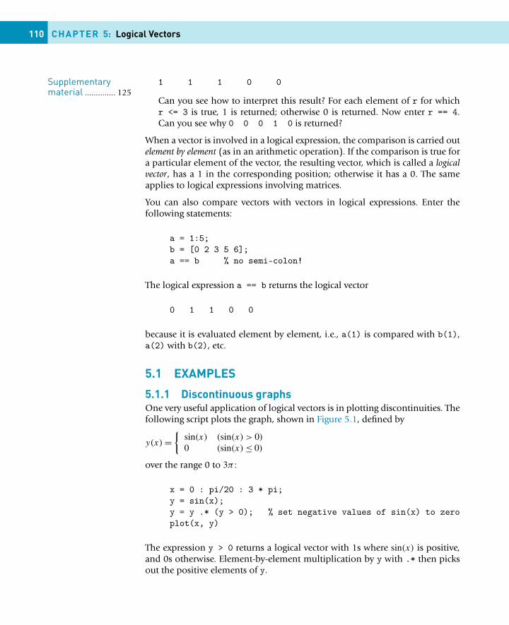
Supplementarymaterial .............. 125
110 CHAPTER 5: Logical Vectors
1 1 1 0 0
Can you see how to interpret this result? For each element of r for whichr <= 3 is true, 1 is returned; otherwise 0 is returned. Now enter r == 4.Can you see why 0 0 0 1 0 is returned?
When a vector is involved in a logical expression, the comparison is carried outelement by element (as in an arithmetic operation). If the comparison is true fora particular element of the vector, the resulting vector, which is called a logicalvector, has a 1 in the corresponding position; otherwise it has a 0. The sameapplies to logical expressions involving matrices.
You can also compare vectors with vectors in logical expressions. Enter thefollowing statements:
a = 1:5;b = [0 2 3 5 6];a == b % no semi-colon!
The logical expression a == b returns the logical vector
0 1 1 0 0
because it is evaluated element by element, i.e., a(1) is compared with b(1),a(2) with b(2), etc.
5.1 EXAMPLES
5.1.1 Discontinuous graphsOne very useful application of logical vectors is in plotting discontinuities. Thefollowing script plots the graph, shown in Figure 5.1, defined by
y(x) ={
sin(x) (sin(x) > 0)
0 (sin(x) ≤ 0)
over the range 0 to 3π :
x = 0 : pi/20 : 3 * pi;y = sin(x);y = y .* (y > 0); % set negative values of sin(x) to zeroplot(x, y)
The expression y > 0 returns a logical vector with 1s where sin(x) is positive,and 0s otherwise. Element-by-element multiplication by y with .* then picksout the positive elements of y.
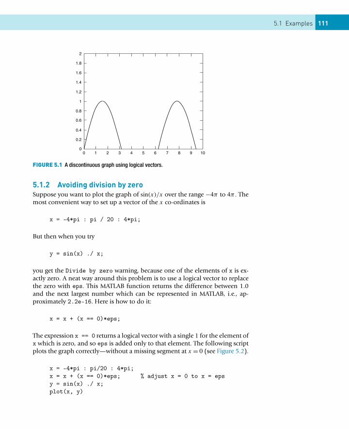
5.1 Examples 111
FIGURE 5.1 A discontinuous graph using logical vectors.
5.1.2 Avoiding division by zeroSuppose you want to plot the graph of sin(x)/x over the range −4π to 4π . Themost convenient way to set up a vector of the x co-ordinates is
x = -4*pi : pi / 20 : 4*pi;
But then when you try
y = sin(x) ./ x;
you get the Divide by zero warning, because one of the elements of x is ex-actly zero. A neat way around this problem is to use a logical vector to replacethe zero with eps. This MATLAB function returns the difference between 1.0and the next largest number which can be represented in MATLAB, i.e., ap-proximately 2.2e-16. Here is how to do it:
x = x + (x == 0)*eps;
The expression x == 0 returns a logical vector with a single 1 for the element ofx which is zero, and so eps is added only to that element. The following scriptplots the graph correctly—without a missing segment at x = 0 (see Figure 5.2).
x = -4*pi : pi/20 : 4*pi;x = x + (x == 0)*eps; % adjust x = 0 to x = epsy = sin(x) ./ x;plot(x, y)
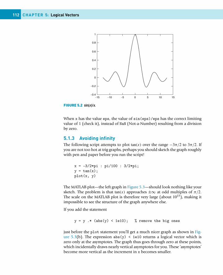
112 CHAPTER 5: Logical Vectors
FIGURE 5.2 sin(x )/x.
When x has the value eps, the value of sin(eps)/eps has the correct limitingvalue of 1 (check it), instead of NaN (Not-a-Number) resulting from a divisionby zero.
5.1.3 Avoiding infinityThe following script attempts to plot tan(x) over the range −3π/2 to 3π/2. Ifyou are not too hot at trig graphs, perhaps you should sketch the graph roughlywith pen and paper before you run the script!
x = -3/2*pi : pi/100 : 3/2*pi;y = tan(x);plot(x, y)
The MATLAB plot—the left graph in Figure 5.3—should look nothing like yoursketch. The problem is that tan(x) approaches ±∞ at odd multiples of π/2.The scale on the MATLAB plot is therefore very large (about 1015), making itimpossible to see the structure of the graph anywhere else.
If you add the statement
y = y .* (abs(y) < 1e10); % remove the big ones
just before the plot statement you’ll get a much nicer graph as shown in Fig-ure 5.3(b). The expression abs(y) < 1e10 returns a logical vector which iszero only at the asymptotes. The graph thus goes through zero at these points,which incidentally draws nearly vertical asymptotes for you. These ‘asymptotes’become more vertical as the increment in x becomes smaller.
5.1 Examples 113
FIGURE 5.3 Variations on tan(x ): (a) Unresticted vertical coordinate. (b) Restricted vertical coor-dinate.
5.1.4 Counting random numbersThe function rand returns a (pseudo-)random number in the interval [0, 1);rand(1, n) returns a row vector of n such numbers. Work out the followingproblem on the command line:
1. Set up a vector r with seven random elements (leave out the semi-colon sothat you can see its elements):
r = rand(1,7) % no semi-colon
Check that the logical expression r < 0.5 gives the correct logical vector.2. Using the function sum on the logical expression r < 0.5 will effectively
count how many elements of r are less than 0.5. Try it, and check youranswer against the values displayed for r:
sum( r < 0.5 )
3. Now use a similar statement to count how many elements of r are greaterthan or equal to 0.5 (the two answers should add up to 7, shouldn’t they?).
4. Since rand generates uniformly distributed random numbers, you would ex-pect the number of random numbers which are less than 0.5 to get closerand closer to half the total number as more and more are generated.Generate a vector of a few thousand random numbers (suppress displaywith a semi-colon this time) and use a logical vector to count how manyare less than 0.5.Repeat a few times with a new set of random numbers each time. Becausethe numbers are random, you should never get quite the same answer eachtime.
Without logical vectors this problem is a little more involved. Here is the pro-gram:
tic % starta = 0; % number >= 0.5b = 0; % number < 0.5
114 CHAPTER 5: Logical Vectors
for n = 1:5000r = rand; % generate one number per loopif r >= 0.5
a = a + 1;else
b = b + 1;end;
end;
t = toc; % finishdisp( [’less than 0.5: ’ num2str(a)] )disp( [’time: ’ num2str(t)] )
It also takes a lot longer. Compare times for the two methods on your com-puter.
5.1.5 Rolling diceWhen a fair dice is rolled, the number uppermost is equally likely to be any in-teger from 1 to 6. So if rand is a random number in the range [0, 1), 6 * randwill be in the range [0, 6), and 6 * rand + 1 will be in the range [1, 7), i.e.,between 1 and 6.9999. Discarding the decimal part of this expression withfloor gives an integer in the required range. Try the following exercises:
1. Generate a vector d of 20 random integers in the range 1 to 6:
d = floor(6 * rand(1, 20)) + 1
2. Count the number of ‘sixes’ thrown by summing the elements of the logicalvector d == 6.
3. Verify your result by displaying d.4. Estimate the probability of throwing a six by dividing the number of sixes
thrown by 20. Using random numbers like this to mimic a real situationbased on chance is called simulation.
5. Repeat with more random numbers in the vector d. The more you have,the closer the proportion of sixes gets to the theoretical expected value of0.1667, i.e., 1/6.
6. Can you see why it would be incorrect to use round instead of floor? Theproblem is that round rounds in both directions, whereas floor roundseverything down.
5.2 LOGICAL OPERATORS
We saw briefly in Chapter 2 that logical expressions can be constructed notonly from the six relational operators, but also from the three logical opera-tors shown in Table 5.1. Table 5.2 shows the effects of these operators on thegeneral logical expressions lex1 and lex2.
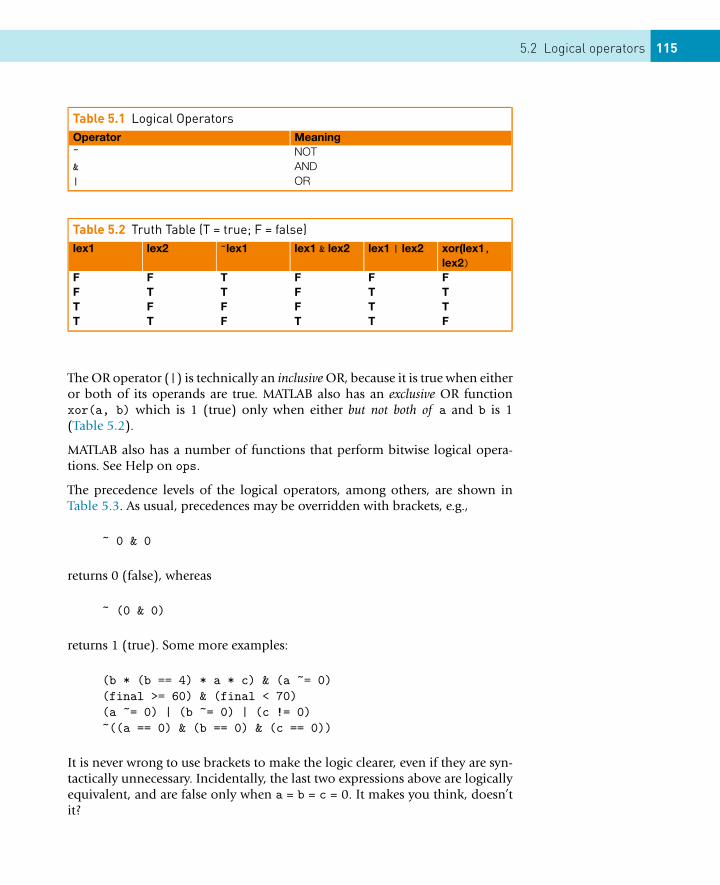
5.2 Logical operators 115
Table 5.1 Logical OperatorsOperator Meaning~ NOT& AND| OR
Table 5.2 Truth Table (T = true; F = false)lex1 lex2 ~lex1 lex1 & lex2 lex1 | lex2 xor(lex1,
lex2)F F T F F FF T T F T TT F F F T TT T F T T F
The OR operator (|) is technically an inclusive OR, because it is true when eitheror both of its operands are true. MATLAB also has an exclusive OR functionxor(a, b) which is 1 (true) only when either but not both of a and b is 1(Table 5.2).
MATLAB also has a number of functions that perform bitwise logical opera-tions. See Help on ops.
The precedence levels of the logical operators, among others, are shown inTable 5.3. As usual, precedences may be overridden with brackets, e.g.,
~ 0 & 0
returns 0 (false), whereas
~ (0 & 0)
returns 1 (true). Some more examples:
(b * (b == 4) * a * c) & (a ~= 0)(final >= 60) & (final < 70)(a ~= 0) | (b ~= 0) | (c != 0)~((a == 0) & (b == 0) & (c == 0))
It is never wrong to use brackets to make the logic clearer, even if they are syn-tactically unnecessary. Incidentally, the last two expressions above are logicallyequivalent, and are false only when a = b = c = 0. It makes you think, doesn’tit?
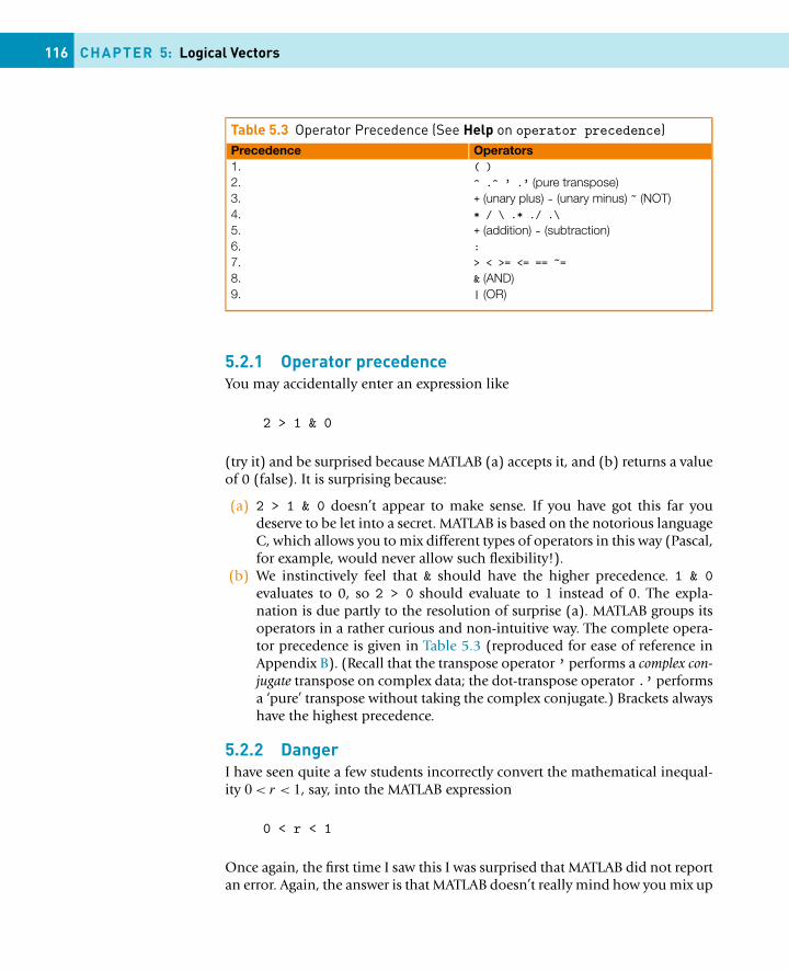
116 CHAPTER 5: Logical Vectors
Table 5.3 Operator Precedence (See Help on operator precedence)Precedence Operators1. ( )2. ^ .^ ’ .’ (pure transpose)3. + (unary plus) - (unary minus) ~ (NOT)4. * / \ .* ./ .\5. + (addition) - (subtraction)6. :7. > < >= <= == ~=8. & (AND)9. | (OR)
5.2.1 Operator precedenceYou may accidentally enter an expression like
2 > 1 & 0
(try it) and be surprised because MATLAB (a) accepts it, and (b) returns a valueof 0 (false). It is surprising because:
(a) 2 > 1 & 0 doesn’t appear to make sense. If you have got this far youdeserve to be let into a secret. MATLAB is based on the notorious languageC, which allows you to mix different types of operators in this way (Pascal,for example, would never allow such flexibility!).
(b) We instinctively feel that & should have the higher precedence. 1 & 0evaluates to 0, so 2 > 0 should evaluate to 1 instead of 0. The expla-nation is due partly to the resolution of surprise (a). MATLAB groups itsoperators in a rather curious and non-intuitive way. The complete opera-tor precedence is given in Table 5.3 (reproduced for ease of reference inAppendix B). (Recall that the transpose operator ’ performs a complex con-jugate transpose on complex data; the dot-transpose operator .’ performsa ‘pure’ transpose without taking the complex conjugate.) Brackets alwayshave the highest precedence.
5.2.2 DangerI have seen quite a few students incorrectly convert the mathematical inequal-ity 0 < r < 1, say, into the MATLAB expression
0 < r < 1
Once again, the first time I saw this I was surprised that MATLAB did not reportan error. Again, the answer is that MATLAB doesn’t really mind how you mix up
5.2 Logical operators 117
operators in an expression. It simply churns through the expression accordingto its rules (which may not be what you expect).
Suppose r has the value 0.5. Mathematically, the inequality is true for this valueof r since it lies in the required range. However, the expression 0 < r < 1is evaluated as 0. This is because the left hand operation (0 < 0.5) is firstevaluated to 1 (true), followed by 1 < 1 which is false.
Inequalities like this should rather be coded as
(0 < r) & (r < 1)
The brackets are not strictly necessary (see Table 5.3) but they certainly help toclarify the logic.
5.2.3 Logical operators and vectorsThe logical operators can also operate on vectors (of the same size), returninglogical vectors, e.g.,
~(~[1 2 0 -4 0])
replaces all the non-zeros by 1s, and leaves the 0s untouched. Try it.
The script in Section 5.1 that avoids division by zero has the critical statement
x = x + (x == 0)*eps;
This is equivalent to
x = x + (~x)*eps;
Try it, and make sure you understand how it works.
Exercises
Work out the results of the following expressions before checking them at thecommand line:
a = [-1 0 3];b = [0 3 1];~aa & ba | bxor(a, b)a > 0 & b > 0
118 CHAPTER 5: Logical Vectors
a > 0 | b > 0~ a > 0a + (~ b)a > ~ b~ a > b~ (a > b)
5.3 SUBSCRIPTING WITH LOGICAL VECTORS
We saw briefly in Chapter 2 that elements of a vector may be referenced withsubscripts, and that the subscripts themselves may be vectors, e.g.,
a = [-2 0 1 5 9];a([5 1 3])
returns
9 -2 1
i.e., the fifth, first and third elements of a. In general, if x and v are vectors,where v has n elements, then x(v) means
[x(v(1)), x(v(2)), ..., x(v(n))]
Now with a as defined above, see what
a(logical([0 1 0 1 0]))
returns. The function logical(v) returns a logical vector, with elements whichare 1 or 0 according as the elements of v are non-zero or 0.
A summary of the rules for the use of a logical vector as a subscript are asfollows:
� A logical vector v may be a subscript of another vector x.� Only the elements of x corresponding to 1s in v are returned.� x and v must be the same size.
Thus, the statement above returns
0 5
i.e., the second and fourth elements of a, corresponding to the 1s inlogical([0 1 0 1 0]).
5.4 Logical functions 119
What will
a(logical([1 1 1 0 0]))
return? And what about a(logical([0 0 0 0 0]))?
Logical vector subscripts provide an elegant way of removing certain elementsfrom a vector, e.g.,
a = a(a > 0)
removes all the non-positive elements from a, because a > 0 returns the log-ical vector [0 0 1 1 1]. We can verify incidentally that the expression a > 0is a logical vector, because the statement
islogical(a > 0)
returns 1. However, the numeric vector [0 0 1 1 1] is not a logical vector; thestatement
islogical([0 0 1 1 1])
returns 0.
5.4 LOGICAL FUNCTIONS
MATLAB has a number of useful logical functions that operate on scalars, vec-tors and matrices. Examples are given in the following list (where x is a vectorunless otherwise stated). See Help on logical functions. (The functions aredefined slightly differently for matrix arguments—see Chapter 6 or Help.)
any(x) returns the scalar 1 (true) if any element of x is non-zero (true).
all(x) returns the scalar 1 if all the elements of x are non-zero.
exist(’a’) returns 1 if a is a workspace variable. For other possible returnvalues see help. Note that a must be enclosed in apostrophes.
find(x) returns a vector containing the subscripts of the non-zero (true) ele-ments of x, so for example,
a = a( find(a) )
removes all the zero elements from a! Try it. Another use of find is in findingthe subscripts of the largest (or smallest) elements in a vector, when there ismore than one. Enter the following:
120 CHAPTER 5: Logical Vectors
x = [8 1 -4 8 6];find(x >= max(x))
This returns the vector [1 4], which are the subscripts of the largest ele-ment (8). It works because the logical expression x >= max(x) returns a logicalvector with 1s only at the positions of the largest elements.
isempty(x) returns 1 if x is an empty array and 0 otherwise. An empty arrayhas a size of 0-by-0.
isinf(x) returns 1s for the elements of x which are +Inf or −Inf, and 0sotherwise.
isnan(x) returns 1s where the elements of x are NaN and 0s otherwise. Thisfunction may be used to remove NaNs from a set of data. This situation couldarise while you are collecting statistics; missing or unavailable values can betemporarily represented by NaNs. However, if you do any calculations involvingthe NaNs, they propagate through intermediate calculations to the final result.To avoid this, the NaNs in a vector may be removed with a statement like
x(isnan(x)) = [ ]
MATLAB has a number of other logical functions starting with the charactersis. See is* in the Help index for the complete list.
5.4.1 Using any and allBecause any and all with vector arguments return scalars, they are particularlyuseful in if statements. For example,
if all(a >= 1)do something
end
means ‘if all the elements of the vector a are greater than or equal to 1, then dosomething’.
Recall from Chapter 2 that a vector condition in an if statement is true only ifall its elements are non-zero. So if you want to execute statement below whentwo vectors a and b are equal (i.e., the same) you could say
if a == bstatement
end
since if considers the logical vector returned by a == b true only if every ele-ment is a 1.
If, on the other hand, you want to execute statement specifically when the vec-tors a and b are not equal, the temptation is to say
5.5 Logical vectors instead of elseif ladders 121
if a ~= b % wrong wrong wrong!!!statement
end
However this will not work, since statement will only execute if each of the cor-responding elements of a and b differ. This is where any comes in:
if any(a ~= b) % right right right!!!statement
end
This does what is required since any(a ~= b) returns the scalar 1 if any ele-ment of a differs from the corresponding element of b.
5.5 LOGICAL VECTORS INSTEAD OF elseif LADDERSThose of us who grew up on more conventional programming languages inthe last century may find it difficult to think in terms of using logical vectorswhen solving general problems. It’s a nice challenge whenever writing a pro-gram to ask yourself whether you can possibly use logical vectors. They arealmost always faster than other methods, although often not as clear to readlater. You must decide when it’s important for you to use logical vectors. But it’sa very good programming exercise to force yourself to use them whenever pos-sible! The following example illustrates these points by first solving a problemconventionally, and then with logical vectors.
It has been said that there are two unpleasant and unavoidable facts of life:death and income tax. A very simplified version of how income tax is calculatedcould be based on the following table:
Taxable income Tax payable$10 000 or less 10% of taxable incomeBetween $10 000 and $20 000 $1000 + 20% of amount by which
taxable income exceeds $10 000More than $20 000 $3000 + 50% of amount by which
taxable income exceeds $20 000
The tax payable on a taxable income of $30 000, for example, is
$3000 + 50% of ($30 000 − $20 000), i.e., $8000.
We would like to calculate the income tax on the following taxable incomes(in dollars): 5000, 10 000, 15 000, 30 000 and 50 000.
The conventional way to program this problem is to set up a vector with thetaxable incomes as elements and to use a loop with an elseif ladder to pro-cess each element, as follows:
122 CHAPTER 5: Logical Vectors
% Income tax the old-fashioned way
inc = [5000 10000 15000 30000 50000];
for ti = inc
if ti < 10000tax = 0.1 * ti;
elseif ti < 20000tax = 1000 + 0.2 * (ti - 10000);
elsetax = 3000 + 0.5 * (ti - 20000);
end;
disp( [ti tax] )end;
Here is the output, suitably edited (note that the amount of tax paid changescontinuously between tax ‘brackets’—each category of tax is called a bracket):
Taxable income Income tax
5000.00 500.0010000.00 1000.0015000.00 2000.0030000.00 8000.0050000.00 18000.00
Now here is the logical way:
% Income tax the logical way
inc = [5000 10000 15000 30000 50000];
tax = 0.1 * inc .* (inc <= 10000);tax = tax + (inc > 10000 & inc <= 20000) ...
.* (0.2 * (inc-10000) + 1000);tax = tax + (inc > 20000) .* (0.5 * (inc-20000) + 3000);
disp( [inc’ tax’] );
To understand how it works, it may help to enter the statements on the com-mand line. Start by entering the vector inc as given. Now enter
inc <= 10000
5.5 Summary 123
which should give the logical vector [1 1 0 0 0]. Next enter
inc .* (inc <= 10000)
which should give the vector [5000 10000 0 0 0]. This has successfully se-lected only the incomes in the first bracket. The tax for these incomes is thencalculated with
tax = 0.1 * inc .* (inc <= 10000)
which returns [500 1000 0 0 0].
Now for the second tax bracket. Enter the expression
inc > 10000 & inc <= 20000
which returns the logical vector [0 0 1 0 0], since there is only one incomein this bracket. Now enter
0.2 * (inc-10000) + 1000
This returns [0 1000 2000 5000 9000]. Only the third entry is correct. Multi-plying this vector by the logical vector just obtained blots out the other entries,giving [0 0 2000 0 0]. The result can be safely added to the vector tax sinceit will not affect the first two entries already there.
I am sure you will agree that the logical vector solution is more interesting thanthe conventional one!
SUMMARY� When a relational and/or logical operator operates on a vector expression,
the operation is carried out element by element. The result is a logical vectorconsisting of 0s (FALSE) and 1s (TRUE).
� A vector may be subscripted with a logical vector of the same size. Only theelements corresponding to the 1s in the logical vector are returned.
� When one of the logical operators (~ & |) operates on an expressionany non-zero value in an operand is regarded as TRUE; zero is regarded asFALSE. A logical vector is returned.
� Arithmetic, relational and logical operators may appear in the same expres-sion. Great care must be taken in observing the correct operator precedencein such situations.
� Vectors in a logical expression must all be the same size.� If a logical expression is a vector or a matrix, it is considered true in an if
statement only if all its elements are non-zero.
124 CHAPTER 5: Logical Vectors
� The logical functions any and all return scalars when taking vector argu-ments, and are consequently useful in if statements.
� Logical vectors may often be used instead of the more conventional elseifladder. This provides faster more elegant code, but requires more ingenuityand the code may be less clear to read later on.
EXERCISES5.1 Determine the values of the following expressions yourself before check-
ing your answers using MATLAB. You may need to consult Table 5.3.(a) 1 & -1(b) 13 & ~(-6)(c) 0 < -2|0(d) ~[1 0 2] * 3(e) 0 <= 0.2 <= 0.4(f) 5 > 4 > 3(g) 2 > 3 & 1
5.2 Given that a = [1 0 2] and b = [0 2 2] determine the values of thefollowing expressions. Check your answers with MATLAB.(a) a ~= b(b) a < b(c) a < b < a(d) a < b < b(e) a | (~a)(f) b & (~b)(g) a(~(~b))(h) a = b == a (determine final value of a)
5.3 Write some MATLAB statements on the command line which use logicalvectors to count how many elements of a vector x are negative, zero orpositive. Check that they work, e.g., with the vector
[-4 0 5 -3 0 3 7 -1 6]
5.4 The Receiver of Revenue (Internal Revenue Service) decides to change thetax table used in Section 5.5 slightly by introducing an extra tax bracketand changing the tax-rate in the third bracket, as shown in the table onthe next page.Amend the logical vector script to handle this table, and test it on thefollowing list of incomes (dollars): 5000, 10 000, 15 000, 22 000, 30 000,38 000 and 50 000.
5.5 A certain company offers seven annual salary levels (dollars): 12 000,15 000, 18 000, 24 000, 35 000, 50 000 and 70 000. The number of em-ployees paid at each level are, respectively: 3000, 2500, 1500, 1000, 400,100 and 25. Write some statements at the command line to find the fol-lowing:
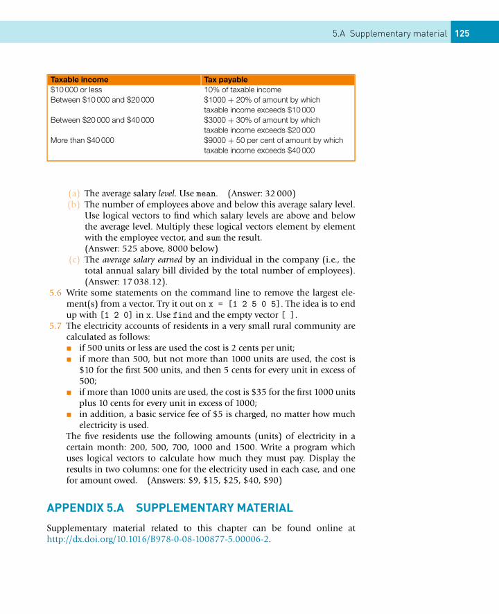
5.A Supplementary material 125
Taxable income Tax payable$10 000 or less 10% of taxable incomeBetween $10 000 and $20 000 $1000 + 20% of amount by which
taxable income exceeds $10 000Between $20 000 and $40 000 $3000 + 30% of amount by which
taxable income exceeds $20 000More than $40 000 $9000 + 50 per cent of amount by which
taxable income exceeds $40 000
(a) The average salary level. Use mean. (Answer: 32 000)(b) The number of employees above and below this average salary level.
Use logical vectors to find which salary levels are above and belowthe average level. Multiply these logical vectors element by elementwith the employee vector, and sum the result.(Answer: 525 above, 8000 below)
(c) The average salary earned by an individual in the company (i.e., thetotal annual salary bill divided by the total number of employees).(Answer: 17 038.12).
5.6 Write some statements on the command line to remove the largest ele-ment(s) from a vector. Try it out on x = [1 2 5 0 5]. The idea is to endup with [1 2 0] in x. Use find and the empty vector [ ].
5.7 The electricity accounts of residents in a very small rural community arecalculated as follows:� if 500 units or less are used the cost is 2 cents per unit;� if more than 500, but not more than 1000 units are used, the cost is
$10 for the first 500 units, and then 5 cents for every unit in excess of500;
� if more than 1000 units are used, the cost is $35 for the first 1000 unitsplus 10 cents for every unit in excess of 1000;
� in addition, a basic service fee of $5 is charged, no matter how muchelectricity is used.
The five residents use the following amounts (units) of electricity in acertain month: 200, 500, 700, 1000 and 1500. Write a program whichuses logical vectors to calculate how much they must pay. Display theresults in two columns: one for the electricity used in each case, and onefor amount owed. (Answers: $9, $15, $25, $40, $90)
APPENDIX 5.A SUPPLEMENTARY MATERIAL
Supplementary material related to this chapter can be found online athttp://dx.doi.org/10.1016/B978-0-08-100877-5.00006-2.
CONTENTS
Matrices .............. 127A concreteexample ................. 127Creating matrices.. 129Subscripts ............. 129Transpose.............. 130The colon operator 130Duplicating rows andcolumns: tiling ...... 133Deleting rows andcolumns................. 134Elementarymatrices ................ 135Specializedmatrices ................ 136Using MATLABfunctions withmatrices ................ 137Manipulatingmatrices ................ 138Array(element-by-element)operations onmatrices ................ 138Matrices and for ... 139Visualization ofmatrices ................ 140Vectorizing nestedfors: loan repaymenttables..................... 140
CHAPTER 6
Matrices and Arrays
THE OBJECTIVES OF THIS CHAPTER ARE TO:
� Introduce you to ways of creating and manipulating matrices.� Introduce you to matrix operations.� Introduce you to character strings and facilities for handling them.� Demonstrate some uses of matrices by examples in:
– Population dynamics.– Markov processes.– Linear equations.
� Introduce MATLAB’s sparse matrix facilities.
As we have already seen, the name MATLAB stands for MATrix LABoratory,because the MATLAB system is designed specially to work with data arranged inthe form of matrices (2-D arrays). The word ‘matrix’ has two distinct meaningsin this chapter:
1. An arrangement of data in rows and columns, e.g., a table.2. A mathematical object, for which particular mathematical operations are
defined, e.g., ‘matrix’ multiplication.
We begin this chapter (in Sections 6.6.1–6.6.3) by looking at matrices in thefirst sense, summarizing and extending what we learned about them in Chap-ter 2. We then go on to look briefly at the mathematical operations on matrices.Subsequently, we examine how these operations can be applied in a numberof widely differing areas, such as systems of linear equations, population dy-namics, and Markov processes.
6.1 MATRICES
6.1.1 A concrete exampleA ready-mix concrete company has three factories (S1, S2 and S3) which mustsupply three building sites (D1, D2 and D3). The costs, in some suitable cur-
127Essential MATLAB for Engineers and Scientists. DOI:10.1016/B978-0-08-100877-5.00007-4Copyright © 2017 Daniel T. Valentine. Published by Elsevier Ltd. All rights reserved.
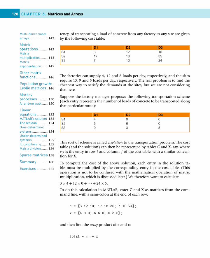
Multi-dimensionalarrays .................... 142
Matrixoperations .......... 143Matrixmultiplication ........ 143Matrixexponentiation....... 145
Other matrixfunctions ............. 146
Population growth:Leslie matrices . 146
Markovprocesses ........... 150A random walk ...... 150
Linearequations ............ 152MATLAB’s solution 153The residual .......... 154Over-determinedsystems ................. 154Under-determinedsystems ................. 155Ill conditioning....... 155Matrix division ....... 156
Sparse matrices 158
Summary ............ 160
Exercises ............ 161
128 CHAPTER 6: Matrices and Arrays
rency, of transporting a load of concrete from any factory to any site are givenby the following cost table:
D1 D2 D3S1 3 12 10S2 17 18 35S3 7 10 24
The factories can supply 4, 12 and 8 loads per day, respectively, and the sitesrequire 10, 9 and 5 loads per day, respectively. The real problem is to find thecheapest way to satisfy the demands at the sites, but we are not consideringthat here.
Suppose the factory manager proposes the following transportation scheme(each entry represents the number of loads of concrete to be transported alongthat particular route):
D1 D2 D3S1 4 0 0S2 6 6 0S3 0 3 5
This sort of scheme is called a solution to the transportation problem. The costtable (and the solution) can then be represented by tables C and X, say, wherecij is the entry in row i and column j of the cost table, with a similar conven-tion for X.
To compute the cost of the above solution, each entry in the solution ta-ble must be multiplied by the corresponding entry in the cost table. (Thisoperation is not to be confused with the mathematical operation of matrixmultiplication, which is discussed later.) We therefore want to calculate
3 × 4 + 12 × 0 + · · · + 24 × 5.
To do this calculation in MATLAB, enter C and X as matrices from the com-mand line, with a semi-colon at the end of each row:
c = [3 12 10; 17 18 35; 7 10 24];
x = [4 0 0; 6 6 0; 0 3 5];
and then find the array product of c and x:
total = c .* x
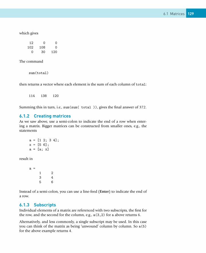
6.1 Matrices 129
which gives
12 0 0102 108 0
0 30 120
The command
sum(total)
then returns a vector where each element is the sum of each column of total:
114 138 120
Summing this in turn, i.e., sum(sum( total )), gives the final answer of 372.
6.1.2 Creating matricesAs we saw above, use a semi-colon to indicate the end of a row when enter-ing a matrix. Bigger matrices can be constructed from smaller ones, e.g., thestatements
a = [1 2; 3 4];x = [5 6];a = [a; x]
result in
a =1 23 45 6
Instead of a semi-colon, you can use a line-feed (Enter) to indicate the end ofa row.
6.1.3 SubscriptsIndividual elements of a matrix are referenced with two subscripts, the first forthe row, and the second for the column, e.g., a(3,2) for a above returns 6.
Alternatively, and less commonly, a single subscript may be used. In this caseyou can think of the matrix as being ‘unwound’ column by column. So a(5)for the above example returns 4.
130 CHAPTER 6: Matrices and Arrays
If you refer to a subscript which is out of range, e.g., a(3,3) for a above, youwill get an error message. However, if you assign a value to an element with asubscript which is out of range the matrix is enlarged to accommodate the newelement, for example, the assignment
a(3,3) = 7
will add a third column to a with 0s everywhere except at a(3,3).
6.1.4 TransposeThe statements
a = [1:3; 4:6]b = a’
result in
a =1 2 34 5 6
b =1 42 53 6
The transpose operator ’ (apostrophe) turns rows into columns and vice versa.
6.1.5 The colon operator� The colon operator is extremely powerful, and provides for very efficient
ways of handling matrices, e.g., if a is the matrix
a =1 2 34 5 67 8 9
the statement
a(2:3,1:2)
results in
4 57 8
6.1 Matrices 131
(returns second and third rows, first and second columns), the statement
a(3,:)
results in
7 8 9
(returns third row), and the statement
a(1:2,2:3) = ones(2)
results in
a =1 1 14 1 17 8 9
(replaces the 2-by-2 submatrix composed of the first and second row andthe second and third column with a square matrix of 1s).Essentially, what is happening in the above examples is that the colon op-erator is being used to create vector subscripts. However, a colon by itself inplace of a subscript denotes all the elements of the corresponding row orcolumn. So a(3,:) means all elements in the third row.This feature may be used, for example, to construct tables. Suppose we wanta table trig of the sines and cosines of the angles 0◦ to 180◦ in steps of 30◦.The following statements achieve this:
x = [0:30:180]’;trig(:,1) = x;trig(:,2) = sin(pi/180*x);trig(:,3) = cos(pi/180*x);
� You can use vector subscripts to get more complicated effects, e.g.,
a(:,[1 3]) = b(:,[4 2])
replaces the first and third columns of a by the fourth and second columnsof b (a and b must have the same number of rows).
� The colon operator is ideal for the sort of row operations performed inGauss reduction (a technique of numerical mathematics), for example, if ais the matrix
a =1 -1 22 1 -13 0 1
132 CHAPTER 6: Matrices and Arrays
the statement
a(2,:) = a(2,:) - a(2,1)*a(1,:)
subtracts the first row multiplied by the first element in the second rowfrom the second row, resulting in
a =1 -1 20 3 -53 0 1
(the idea being to get a zero immediately underneath a(1,1)).� The keyword end refers to the last row or column of an array, for example,
if r is a row vector, the statement
sum(r(3:end))
returns the sum of all the elements of r from the third one to the last one.� The colon operator may also be used as a single subscript, in which case it
behaves differently if it is on the right-hand or left-hand side of an assign-ment. On the right-hand side of an assignment, a(:) gives all the elementsof a strung out by columns in one long column vector, e.g., if
a =1 23 4
the statement
b = a(:)
results in
b =1324
However, on the left-hand side of an assignment, a(:) reshapes a matrix.a must already exist. Then a(:) denotes a matrix with the same dimensions(shape) as a, but with new contents taken from the right-hand side. In otherwords, the matrix on the right-hand side is reshaped into the shape of a onthe left-hand side. Some examples may help. If
b =1 2 34 5 6
6.1 Matrices 133
and
a =0 00 00 0
the statement
a(:) = b
results in
a =1 54 32 6
(the contents of b are strung out into one long column and then fed into aby columns). As another example, the statement
a(:) = 1:6
(with a as above) results in
a =1 42 53 6
Reshaping can also be done with the reshape function. See help.Whether the colon operator appears on the right- or left-hand side of anassignment, the matrices or submatrices on each side of the assignmenthave the same shape (except in the special case below).
� As a special case, a single colon subscript may be used to replace all theelements of a matrix with a scalar, e.g.,
a(:) = -1
6.1.6 Duplicating rows and columns: tilingSometimes it is useful to generate a matrix where all the rows or columns arethe same. This can be done with the repmat function as follows. If a is the rowvector
a =1 2 3
134 CHAPTER 6: Matrices and Arrays
the statement
repmat(a, [3 1])
results in
ans =1 2 31 2 31 2 3
In help’s inimitable phraseology, this statement produces a 3-by-1 ‘tiling’ ofcopies of a. You can think of a as a ‘strip’ of three tiles stuck to self-adhesivebacking. The above statement tiles a floor with three rows and one column ofsuch a strip of tiles.
There is an alternative syntax for repmat:
repmat(a, 3, 1)
An interesting example of this process appears at the end of this section in theloan repayment problem.
6.1.7 Deleting rows and columnsUse the colon operator and the empty array to delete entire rows or columns,for example,
a(:,2) = [ ]
deletes the second column of a.
You can’t delete a single element from a matrix while keeping it a matrix, so astatement like
a(1,2) = [ ]
results in an error. However, using the single subscript notation you can deletea sequence of elements from a matrix and reshape the remaining elements intoa row vector, for example, if
a =1 2 3
6.1 Matrices 135
4 5 67 8 9
the statement
a(2:2:6) = [ ]
results in
a =1 7 5 3 6 9
Get it? (First unwind a by columns, then remove elements 2, 4 and 6.)
You can use logical vectors to extract a selection of rows or columns from a ma-trix, for example, if a is the original 3-by-3 matrix defined above, the statement
a(:, logical([1 0 1]))
results in
ans =1 34 67 9
(first and third columns extracted). The same effect is achieved with
a(:, [1 3])
6.1.8 Elementary matricesThere is a group of functions to generate ‘elementary’ matrices which are usedin a number of applications. See help elmat.
For example, the functions zeros, ones and rand generate matrices of 1s, 0sand random numbers, respectively. With a single argument n, they generaten × n (square) matrices. With two arguments n and m they generate n × m ma-trices. (For very large matrices repmat is usually faster than ones and zeros.)
The function eye(n) generates an n×n identity matrix, i.e., a matrix with 1s onthe main ‘diagonal’, and 0s everywhere else, e.g., the statement
eye(3)
136 CHAPTER 6: Matrices and Arrays
results in
ans =1 0 00 1 00 0 1
(The original version of MATLAB could not use the more obvious name I forthe identity since it did not distinguish between upper- and lowercase lettersand i was the natural choice for the imaginary unit number.)
As an example, eye may be used to construct a tridiagonal matrix as follows.The statements
a = 2 * eye(5);a(1:4, 2:5) = a(1:4, 2:5) - eye(4);a(2:5, 1:4) = a(2:5, 1:4) - eye(4)
result in
a =2 -1 0 0 0
-1 2 -1 0 00 -1 2 -1 00 0 -1 2 -10 0 0 -1 2
Incidentally, if you work with large tridiagonal matrices, you should have alook at the sparse matrix facilities available in MATLAB via the help browser.
6.1.9 Specialized matricesThe following are functions that could be used to generate arbitrary matricesto investigate matrix operations when you cannot think of one to generateyourself. They are special matrices that were discovered by mathematicians,the motivation for their discovery and other details about them you are notexpected to understand.
pascal(n) generates a Pascal matrix of order n. Technically, this is a symmetricpositive definite matrix with entries made up from Pascal’s triangle, e.g.,
pascal(4)
results in
6.1 Matrices 137
ans =1 1 1 11 2 3 41 3 6 101 4 10 20
magic(n) generates an n × n magic square.
MATLAB has a number of other functions which generate special matrices, suchas gallery, hadamard, hankel, hilb, toeplitz, vander, etc. See help elmat.
6.1.10 Using MATLAB functions with matricesWhen a MATLAB mathematical or trigonometric function has a matrix argu-ment, the function operates on every element of the matrix, as you wouldexpect. However, many of the other MATLAB functions operate on matricescolumn by column, e.g., if
a =1 0 11 1 10 0 1
the statement
all(a)
results in
ans =0 0 1
For each column of a where all the elements are true (non-zero) all returns 1,otherwise it returns 0. all therefore returns a logical vector when it takes amatrix argument. To test if all the elements of a are true, use all twice. In thisexample, the statement
all(all(a))
returns 0 because some of the elements of a are 0. On the other hand thestatement
any(a)
138 CHAPTER 6: Matrices and Arrays
returns
ans =1 1 1
because each column of a has at least one non-zero element, and any(any(a))returns 1, since a itself has at least one non-zero element.
If you are not sure whether a particular function operates columnwise or ele-ment by element on matrices, you can always request help.
6.1.11 Manipulating matricesHere are some functions for manipulating matrices. See help for details.
diag extracts or creates a diagonal.
fliplr flips from left to right.
flipud flips from top to bottom.
rot90 rotates.
tril extracts the lower triangular part, e.g., the statement
tril(pascal(4))
results in
ans =1 0 0 01 2 0 01 3 6 01 4 10 20
triu extracts the upper triangular part.
6.1.12 Array (element-by-element) operations on matricesThe array operations discussed in Chapter 2 all apply to matrices as well asvectors. For example, if a is a matrix, a * 2 multiplies each element of a by 2,and if
a =1 2 34 5 6
6.1 Matrices 139
the statement
a .^ 2
results in
ans =1 4 9
16 25 36
6.1.13 Matrices and forIf
a =1 2 34 5 67 8 9
the statements
for v = adisp(v’)
end
result in
1 4 72 5 83 6 9
What happens in this most general form of the for statement is that the indexv takes on the value of each column of the matrix expression a in turn. Thisprovides a neat way of processing all the columns of a matrix. You can do thesame with the rows if you transpose a, e.g., the statements
for v = a’disp(v’)
end
display the rows of a one at a time. Get it?
140 CHAPTER 6: Matrices and Arrays
6.1.14 Visualization of matricesMatrices can be visualized graphically in MATLAB. This subject is discussedbriefly in Chapter 9, with illustrations.
6.1.15 Vectorizing nested fors: loan repayment tablesIf a regular fixed payment P is made n times a year to repay a loan of amountA over a period of k years, where the nominal annual interest rate is r , P isgiven by
P = rA(1 + r/n)nk
n[(1 + r/n)nk − 1] .
We would like to generate a table of repayments for a loan of $1 000 over 15,20 or 25 years, at interest rates that vary from 10% to 20% per annum, insteps of 1%. Since P is directly proportional to A in the above formula, therepayments of a loan of any amount can be found by simple proportion fromsuch a table.
The conventional way of handling this is with ‘nested’ fors. The fprintf state-ments are necessary in order to get the output for each interest rate on the sameline (see MATLAB Help):
A = 1000; % amount borrowedn = 12; % number of payments per year
for r = 0.1 : 0.01 : 0.2fprintf( ’%4.0f%’, 100 * r );for k = 15 : 5 : 25
temp = (1 + r/n) ^ (n*k);P = r * A * temp / (n * (temp - 1));fprintf( ’%10.2f’, P );
end;fprintf( ’\n’ ); % new line
end;
Some sample output (with headings edited in):
rate % 15 yrs 20 yrs 25 yrs
10 10.75 9.65 9.0911 11.37 10.32 9.80...19 16.83 16.21 15.9820 17.56 16.99 16.78
6.1 Matrices 141
However, we saw in Chapter 2 that for loops can often be vectorized, savinga lot of computing time (and also providing an interesting intellectual chal-lenge!). The inner loop can easily be vectorized; the following code uses onlyone for:
...for r = 0.1 : 0.01 : 0.2
k = 15 : 5 : 25;temp = (1 + r/n) .^ (n*k);P = r * A * temp / n ./ (temp - 1);disp( [100 * r, P] );
end;
Note the use of the array operators.
The really tough challenge, however, is to vectorize the outer loop as well. Wewant a table with 11 rows and 3 columns. Start by assigning values to A and n(from the command line):
A = 1000;n = 12;
Then generate a column vector for the interest rates:
r = [0.1:0.01:0.2]’
Now change this into a table with 3 columns each equal to r:
r = repmat(r, [1 3])
The matrix r should look like this:
0.10 0.10 0.100.11 0.11 0.11...0.19 0.19 0.190.20 0.20 0.20
Now do a similar thing for the repayment periods k. Generate the row vector
k = 15:5:25
142 CHAPTER 6: Matrices and Arrays
and expand it into a table with 11 rows each equal to k:
k = repmat(k, [11 1])
This should give you
15 20 2515 20 25...15 20 2515 20 25
The formula for P is a little complicated, so let’s do it in two steps:
temp = (1 + r/n) .^ (n * k);P = r * A .* temp / n ./ (temp - 1)
Finally, you should get this for P:
10.75 9.65 9.0911.37 10.32 9.80...16.83 16.21 15.9817.56 16.99 16.78
This works, because of the way the tables r and k have been constructed, andbecause the MATLAB array operations are performed element by element. Forexample, when the calculation is made for P in row 2 and column 1, the arrayoperations pick out row 2 of r (all 0.11) and column 1 of k (all 15), giving thecorrect value for P (11.37).
The nested for way might be easier to program, but this way is certainly moreinteresting (and quicker to execute).
6.1.16 Multi-dimensional arraysMATLAB arrays can have more than two dimensions. For example, suppose youcreate the matrix
a = [1:2; 3:4]
You can add a third dimension to a with
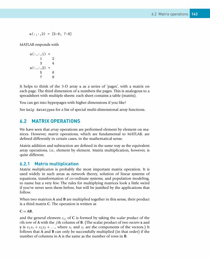
6.2 Matrix operations 143
a(:,:,2) = [5:6; 7:8]
MATLAB responds with
a(:,:,1) =1 23 4
a(:,:,2) =5 67 8
It helps to think of the 3-D array a as a series of ‘pages’, with a matrix oneach page. The third dimension of a numbers the pages. This is analogous to aspreadsheet with multiple sheets: each sheet contains a table (matrix).
You can get into hyperpages with higher dimensions if you like!
See help datatypes for a list of special multi-dimensional array functions.
6.2 MATRIX OPERATIONS
We have seen that array operations are performed element by element on ma-trices. However, matrix operations, which are fundamental to MATLAB, aredefined differently in certain cases, in the mathematical sense.
Matrix addition and subtraction are defined in the same way as the equivalentarray operations, i.e., element by element. Matrix multiplication, however, isquite different.
6.2.1 Matrix multiplicationMatrix multiplication is probably the most important matrix operation. It isused widely in such areas as network theory, solution of linear systems ofequations, transformation of co-ordinate systems, and population modeling,to name but a very few. The rules for multiplying matrices look a little weirdif you’ve never seen them before, but will be justified by the applications thatfollow.
When two matrices A and B are multiplied together in this sense, their productis a third matrix C. The operation is written as
C = AB,
and the general element cij of C is formed by taking the scalar product of theith row of A with the j th column of B. (The scalar product of two vectors x andy is x1y1 + x2y2 + . . ., where xi and yi are the components of the vectors.) Itfollows that A and B can only be successfully multiplied (in that order) if thenumber of columns in A is the same as the number of rows in B.
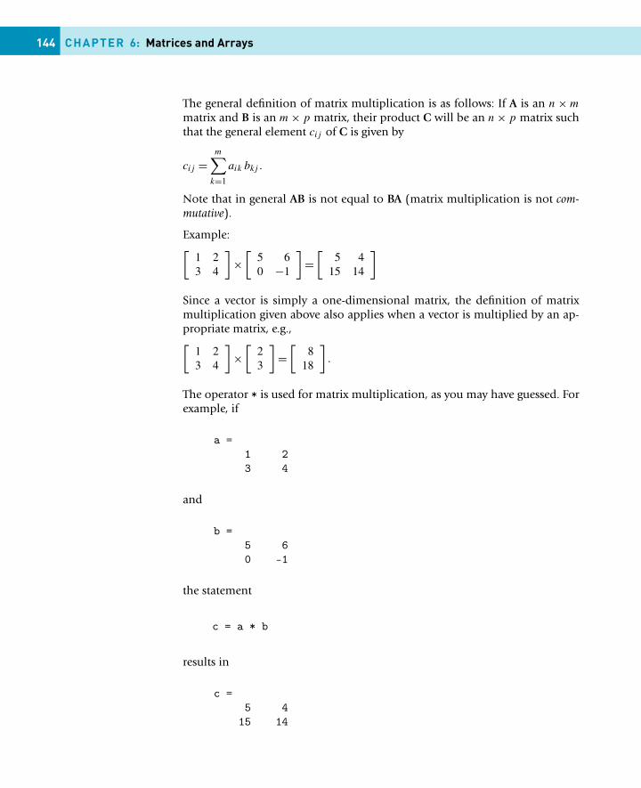
144 CHAPTER 6: Matrices and Arrays
The general definition of matrix multiplication is as follows: If A is an n × m
matrix and B is an m × p matrix, their product C will be an n × p matrix suchthat the general element cij of C is given by
cij =m∑
k=1
aik bkj .
Note that in general AB is not equal to BA (matrix multiplication is not com-mutative).
Example:[1 23 4
]×
[5 60 −1
]=
[5 4
15 14
]
Since a vector is simply a one-dimensional matrix, the definition of matrixmultiplication given above also applies when a vector is multiplied by an ap-propriate matrix, e.g.,[
1 23 4
]×
[23
]=
[8
18
].
The operator * is used for matrix multiplication, as you may have guessed. Forexample, if
a =1 23 4
and
b =5 60 -1
the statement
c = a * b
results in
c =5 4
15 14
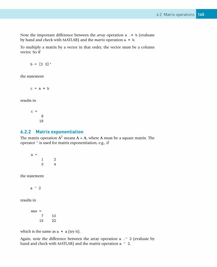
6.2 Matrix operations 145
Note the important difference between the array operation a .* b (evaluateby hand and check with MATLAB) and the matrix operation a * b.
To multiply a matrix by a vector in that order, the vector must be a columnvector. So if
b = [2 3]’
the statement
c = a * b
results in
c =8
18
6.2.2 Matrix exponentiationThe matrix operation A2 means A × A, where A must be a square matrix. Theoperator ^ is used for matrix exponentiation, e.g., if
a =1 23 4
the statement
a ^ 2
results in
ans =7 10
15 22
which is the same as a * a (try it).
Again, note the difference between the array operation a .^ 2 (evaluate byhand and check with MATLAB) and the matrix operation a ^ 2.
146 CHAPTER 6: Matrices and Arrays
6.3 OTHER MATRIX FUNCTIONS
Here are some of MATLAB’s more advanced matrix functions.
det determinant.
eig eigenvalue decomposition.
expm matrix exponential, i.e., eA, where A is a matrix. The matrix exponen-tial may be used to evaluate analytical solutions of linear ordinary differentialequations with constant coefficients.
inv inverse.
lu LU factorization (into lower and upper triangular matrices).
qr orthogonal factorization.
svd singular value decomposition.
6.4 POPULATION GROWTH: LESLIE MATRICES
Our first application of matrices is in population dynamics.
Suppose we want to model the growth of a population of rabbits, in the sensethat given their number at some moment, we would like to estimate the size ofthe population in a few years’ time. One approach is to divide the rabbit pop-ulation up into a number of age classes, where the members of each age classare one time unit older than the members of the previous class, the time unitbeing whatever is convenient for the population being studied (days, months,etc.).
If Xi is the size of the ith age class, we define a survival factor Pi as the propor-tion of the ith class that survive to the (i + 1)th age class, i.e. the proportionthat ‘graduate’. Fi is defined as the mean fertility of the ith class. This is the meannumber of newborn individuals expected to be produced during one time in-terval by each member of the ith class at the beginning of the interval (onlyfemales count in biological modeling, since there are always enough males togo round!).
Suppose for our modified rabbit model we have three age classes, with X1,X2 and X3 members, respectively. We will call them young, middle-aged andold-aged for convenience. We will take our time unit as one month, so X1is the number that were born during the current month, and which will beconsidered as youngsters at the end of the month. X2 is the number of middle-aged rabbits at the end of the month, and X3 the number of oldsters. Supposethe youngsters cannot reproduce, so that F1 = 0. Suppose the fertility rate formiddle-aged rabbits is 9, so F2 = 9, while for oldsters F3 = 12. The probabilityof survival from youth to middle-age is one third, so P1 = 1/3, while no less
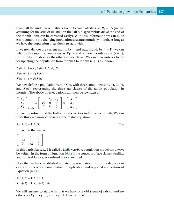
6.4 Population growth: Leslie matrices 147
than half the middle-aged rabbits live to become oldsters, so P2 = 0.5 (we areassuming for the sake of illustration that all old-aged rabbits die at the end ofthe month—this can be corrected easily). With this information we can quiteeasily compute the changing population structure month by month, as long aswe have the population breakdown to start with.
If we now denote the current month by t , and next month by (t + 1), we canrefer to this month’s youngsters as X1(t), and to next month’s as X1(t + 1),with similar notation for the other two age classes. We can then write a schemefor updating the population from month t to month (t + 1) as follows:
X1(t + 1) = F2X2(t) + F3X3(t),
X2(t + 1) = P1X1(t),
X3(t + 1) = P2X2(t).
We now define a population vector X(t), with three components, X1(t), X2(t),and X3(t), representing the three age classes of the rabbit population inmonth t . The above three equations can then be rewritten as⎡⎣ X1
X2X3
⎤⎦
(t+1)
=⎡⎣ 0 F2 F3
P1 0 00 P2 0
⎤⎦ ×
⎡⎣ X1
X2X3
⎤⎦
t
where the subscript at the bottom of the vectors indicates the month. We canwrite this even more concisely as the matrix equation
X(t + 1) = L X(t), (6.1)
where L is the matrix⎡⎣ 0 9 12
1/3 0 00 1/2 0
⎤⎦
in this particular case. L is called a Leslie matrix. A population model can alwaysbe written in the form of Equation (6.1) if the concepts of age classes, fertility,and survival factors, as outlined above, are used.
Now that we have established a matrix representation for our model, we caneasily write a script using matrix multiplication and repeated application ofEquation (6.1):
X(t + 2) = L X(t + 1),
X(t + 3) = L X(t + 2), etc.
We will assume to start with that we have one old (female) rabbit, and noothers, so X1 = X2 = 0, and X3 = 1. Here is the script:
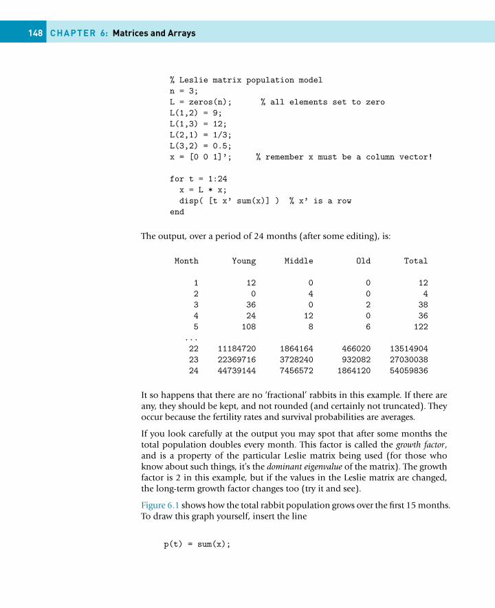
148 CHAPTER 6: Matrices and Arrays
% Leslie matrix population modeln = 3;L = zeros(n); % all elements set to zeroL(1,2) = 9;L(1,3) = 12;L(2,1) = 1/3;L(3,2) = 0.5;x = [0 0 1]’; % remember x must be a column vector!
for t = 1:24x = L * x;disp( [t x’ sum(x)] ) % x’ is a row
end
The output, over a period of 24 months (after some editing), is:
Month Young Middle Old Total
1 12 0 0 122 0 4 0 43 36 0 2 384 24 12 0 365 108 8 6 122
...22 11184720 1864164 466020 1351490423 22369716 3728240 932082 2703003824 44739144 7456572 1864120 54059836
It so happens that there are no ‘fractional’ rabbits in this example. If there areany, they should be kept, and not rounded (and certainly not truncated). Theyoccur because the fertility rates and survival probabilities are averages.
If you look carefully at the output you may spot that after some months thetotal population doubles every month. This factor is called the growth factor,and is a property of the particular Leslie matrix being used (for those whoknow about such things, it’s the dominant eigenvalue of the matrix). The growthfactor is 2 in this example, but if the values in the Leslie matrix are changed,the long-term growth factor changes too (try it and see).
Figure 6.1 shows how the total rabbit population grows over the first 15 months.To draw this graph yourself, insert the line
p(t) = sum(x);
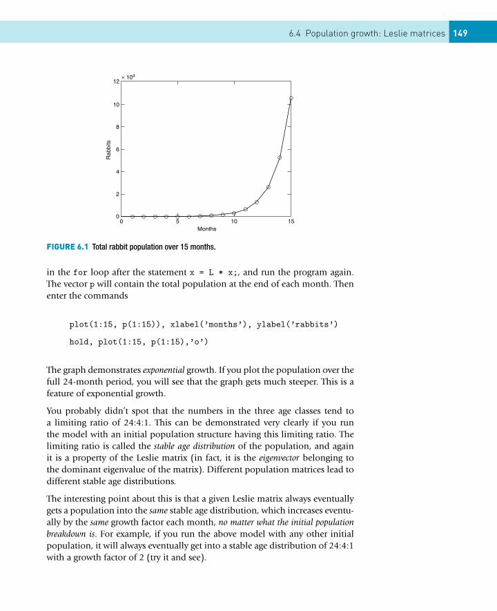
6.4 Population growth: Leslie matrices 149
FIGURE 6.1 Total rabbit population over 15 months.
in the for loop after the statement x = L * x;, and run the program again.The vector p will contain the total population at the end of each month. Thenenter the commands
plot(1:15, p(1:15)), xlabel(’months’), ylabel(’rabbits’)
hold, plot(1:15, p(1:15),’o’)
The graph demonstrates exponential growth. If you plot the population over thefull 24-month period, you will see that the graph gets much steeper. This is afeature of exponential growth.
You probably didn’t spot that the numbers in the three age classes tend toa limiting ratio of 24:4:1. This can be demonstrated very clearly if you runthe model with an initial population structure having this limiting ratio. Thelimiting ratio is called the stable age distribution of the population, and againit is a property of the Leslie matrix (in fact, it is the eigenvector belonging tothe dominant eigenvalue of the matrix). Different population matrices lead todifferent stable age distributions.
The interesting point about this is that a given Leslie matrix always eventuallygets a population into the same stable age distribution, which increases eventu-ally by the same growth factor each month, no matter what the initial populationbreakdown is. For example, if you run the above model with any other initialpopulation, it will always eventually get into a stable age distribution of 24:4:1with a growth factor of 2 (try it and see).
150 CHAPTER 6: Matrices and Arrays
See help eig if you’re interested in using MATLAB to compute eigenvaluesand eigenvectors.
6.5 MARKOV PROCESSES
Often a process that we wish to model may be represented by a number ofpossible discrete (i.e. discontinuous) states that describe the outcome of theprocess. For example, if we are spinning a coin, then the outcome is adequatelyrepresented by the two states ‘heads’ and ‘tails’ (and nothing in between). If theprocess is random, as it is with spinning coins, there is a certain probabilityof being in any of the states at a given moment, and also a probability ofchanging from one state to another. If the probability of moving from onestate to another depends on the present state only, and not on any previousstate, the process is called a Markov chain. The progress of the myopic sailor inChapter 13 is an example of such a process. Markov chains are used widely insuch diverse fields as biology and business decision making, to name just twoareas.
6.5.1 A random walk
This example is a variation on the random walk simulation of Chapter 13.A street has six intersections. A short-sighted student wanders down the street.His home is at intersection 1, and his favorite internet cafe at intersection 6. Ateach intersection other than his home or the cafe he moves in the direction ofthe cafe with probability 2/3, and in the direction of his home with probability1/3. In other words, he is twice as likely to move towards the cafe as towardshis home. He never wanders down a side street. If he reaches his home or thecafe, he disappears into them, never to re-appear (when he disappears we sayin Markov jargon that he has been absorbed).
We would like to know: what are the chances of him ending up at home or inthe cafe, if he starts at a given corner (other than home or the cafe, obviously)?He can clearly be in one of six states, with respect to his random walk, whichcan be labeled by the intersection number, where state 1 means Home and state6 means Cafe. We can represent the probabilities of being in these states by asix-component state vector X(t), where Xi(t) is the probability of him being atintersection i at moment t . The components of X(t) must sum to 1, since hehas to be in one of these states.
We can express this Markov process with the following transition probability ma-trix, P, where the rows represent the next state (i.e. corner), and the columnsrepresent the present state:
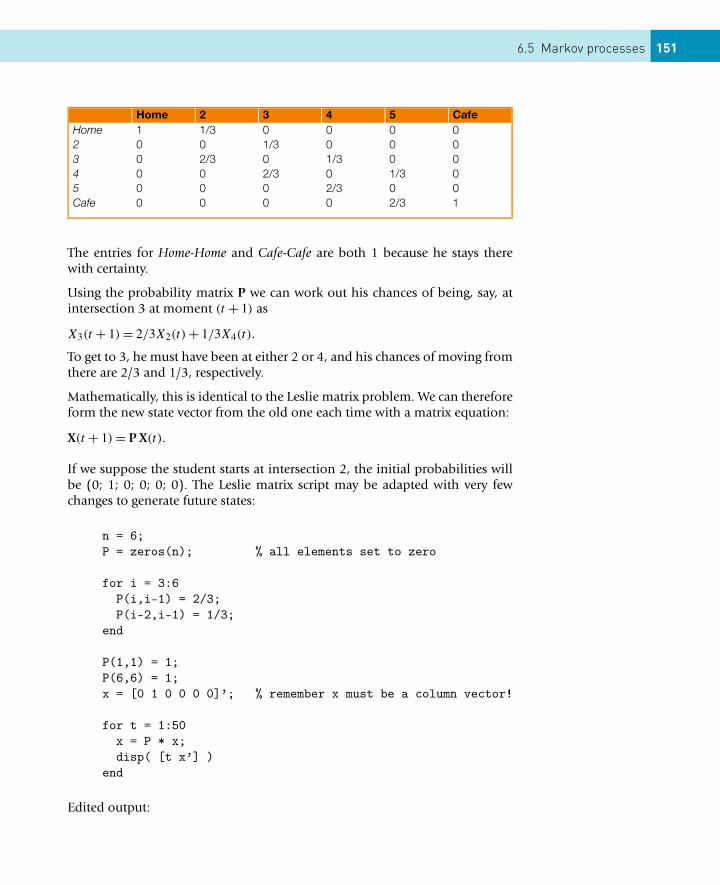
6.5 Markov processes 151
Home 2 3 4 5 CafeHome 1 1/3 0 0 0 02 0 0 1/3 0 0 03 0 2/3 0 1/3 0 04 0 0 2/3 0 1/3 05 0 0 0 2/3 0 0Cafe 0 0 0 0 2/3 1
The entries for Home-Home and Cafe-Cafe are both 1 because he stays therewith certainty.
Using the probability matrix P we can work out his chances of being, say, atintersection 3 at moment (t + 1) as
X3(t + 1) = 2/3X2(t) + 1/3X4(t).
To get to 3, he must have been at either 2 or 4, and his chances of moving fromthere are 2/3 and 1/3, respectively.
Mathematically, this is identical to the Leslie matrix problem. We can thereforeform the new state vector from the old one each time with a matrix equation:
X(t + 1) = P X(t).
If we suppose the student starts at intersection 2, the initial probabilities willbe (0; 1; 0; 0; 0; 0). The Leslie matrix script may be adapted with very fewchanges to generate future states:
n = 6;P = zeros(n); % all elements set to zero
for i = 3:6P(i,i-1) = 2/3;P(i-2,i-1) = 1/3;
end
P(1,1) = 1;P(6,6) = 1;x = [0 1 0 0 0 0]’; % remember x must be a column vector!
for t = 1:50x = P * x;disp( [t x’] )
end
Edited output:
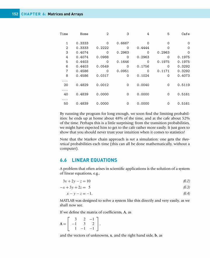
152 CHAPTER 6: Matrices and Arrays
Time Home 2 3 4 5 Cafe
1 0.3333 0 0.6667 0 0 02 0.3333 0.2222 0 0.4444 0 03 0.4074 0 0.2963 0 0.2963 04 0.4074 0.0988 0 0.2963 0 0.19755 0.4403 0 0.1646 0 0.1975 0.19756 0.4403 0.0549 0 0.1756 0 0.32927 0.4586 0 0.0951 0 0.1171 0.32928 0.4586 0.0317 0 0.1024 0 0.4073
...20 0.4829 0.0012 0 0.0040 0 0.5119
...40 0.4839 0.0000 0 0.0000 0 0.5161
...50 0.4839 0.0000 0 0.0000 0 0.5161
By running the program for long enough, we soon find the limiting probabil-ities: he ends up at home about 48% of the time, and at the cafe about 52%of the time. Perhaps this is a little surprising; from the transition probabilities,we might have expected him to get to the cafe rather more easily. It just goes toshow that you should never trust your intuition when it comes to statistics!
Note that the Markov chain approach is not a simulation: one gets the theo-retical probabilities each time (this can all be done mathematically, without acomputer).
6.6 LINEAR EQUATIONS
A problem that often arises in scientific applications is the solution of a systemof linear equations, e.g.,
3x + 2y − z = 10 (6.2)
−x + 3y + 2z = 5 (6.3)
x − y − z = −1. (6.4)
MATLAB was designed to solve a system like this directly and very easily, as weshall now see.
If we define the matrix of coefficients, A, as
A =⎡⎣ 3 2 −1
−1 3 21 −1 −1
⎤⎦ ,
and the vectors of unknowns, x, and the right hand side, b, as
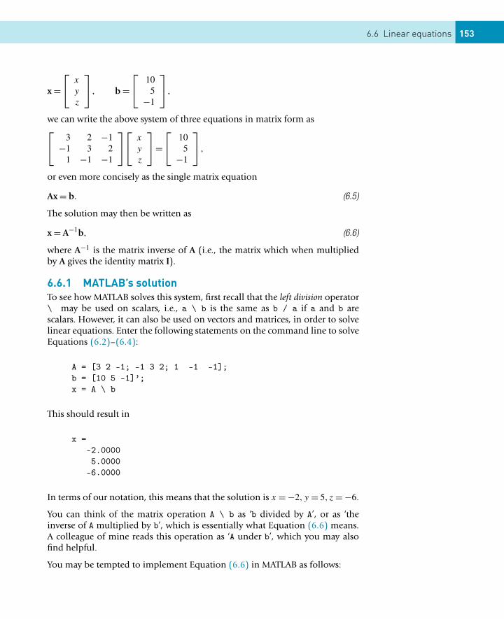
6.6 Linear equations 153
x =⎡⎣ x
y
z
⎤⎦ , b =
⎡⎣ 10
5−1
⎤⎦ ,
we can write the above system of three equations in matrix form as⎡⎣ 3 2 −1
−1 3 21 −1 −1
⎤⎦
⎡⎣ x
y
z
⎤⎦ =
⎡⎣ 10
5−1
⎤⎦ ,
or even more concisely as the single matrix equation
Ax = b. (6.5)
The solution may then be written as
x = A−1b, (6.6)
where A−1 is the matrix inverse of A (i.e., the matrix which when multipliedby A gives the identity matrix I).
6.6.1 MATLAB’s solutionTo see how MATLAB solves this system, first recall that the left division operator\ may be used on scalars, i.e., a \ b is the same as b / a if a and b arescalars. However, it can also be used on vectors and matrices, in order to solvelinear equations. Enter the following statements on the command line to solveEquations (6.2)–(6.4):
A = [3 2 -1; -1 3 2; 1 -1 -1];b = [10 5 -1]’;x = A \ b
This should result in
x =-2.00005.0000
-6.0000
In terms of our notation, this means that the solution is x = −2, y = 5, z = −6.
You can think of the matrix operation A \ b as ‘b divided by A’, or as ‘theinverse of A multiplied by b’, which is essentially what Equation (6.6) means.A colleague of mine reads this operation as ‘A under b’, which you may alsofind helpful.
You may be tempted to implement Equation (6.6) in MATLAB as follows:
154 CHAPTER 6: Matrices and Arrays
x = inv(A) * b
since the function inv finds a matrix inverse directly. However, A \ b is actu-ally more accurate and efficient; see MATLAB Help: Functions — AlphabeticalList and click on inv.
6.6.2 The residualWhenever we solve a system of linear equations numerically we need to havesome idea of how accurate the solution is. The first thing to check is the residual,defined as
r = A*x - b
where x is the result of the operation x = A \ b. Theoretically the residualr should be zero, since the expression A * x is supposed to be equal to b,according to Equation (6.5), which is the equation we are trying to solve. Inour example here the residual is (check it)
r =1.0e-015 *
00.88820.6661
This seems pretty conclusive: all the elements of the residual are less than 10−15
in absolute value. Unfortunately, there may still be problems lurking beneaththe surface, as we shall see shortly.
We will, however, first look at a situation where the residual turns out to be farfrom zero.
6.6.3 Over-determined systemsWhen we have more equations than unknowns, the system is called over-determined, e.g.,
x − y = 0
y = 2
x = 1.
Surprisingly, perhaps, MATLAB gives a solution to such a system. If
A = [1 -1; 0 1; 1 0];b = [0 2 1]’;
6.6 Linear equations 155
the statement
x = A \ b
results in
x =1.33331.6667
The residual r = A*x - b is now
r =-0.3333-0.33330.3333
What happens in this case is that MATLAB produces the least squares best fit.This is the value of x which makes the magnitude of r, i.e.,√r(1)2 + r(2)2 + r(3)3,
as small as possible. You can compute this quantity (0.5774) with sqrt(r’*r)or sqrt(sum(r .* r)). There is a nice example of fitting a decaying exponen-tial function to data with a least squares fit in MATLAB Help: Mathematics:Matrices and Linear Algebra: Solving Linear Equations: OverdeterminedSystems.
6.6.4 Under-determined systemsIf there are fewer equations than unknowns, the system is called under-determined. In this case there are an infinite number of solutions; MATLAB willfind one which has zeros for some of the unknowns.
The equations in such a system are the constraints in a linear programmingproblem.
6.6.5 Ill conditioningSometimes the coefficients of a system of equations are the results of an exper-iment, and may be subject to error. We need in that case to know how sensitivethe solution is to the experimental errors. As an example, consider the system
10x + 7y + 8z + 7w = 32
7x + 5y + 6z + 5w = 23
156 CHAPTER 6: Matrices and Arrays
8x + 6y + 10z + 9w = 33
7x + 5y + 9z + 10w = 31
Use matrix left division to show that the solution is x = y = z = w = 1. Theresidual is exactly zero (check it), and all seems well.
However, if we change the right-hand side constants to 32.1, 22.9, 32.9 and31.1, the ‘solution’ is now given by x = 6, y = −7.2, z = 2.9,w = −0.1. Theresidual is very small.
A system like this is called ill-conditioned, meaning that a small change in the co-efficients leads to a large change in the solution. The MATLAB function rcondreturns the condition estimator, which tests for ill conditioning. If A is the coef-ficient matrix, rcond(A) will be close to zero if A is ill-conditioned, but closeto 1 if it is well-conditioned. In this example, the condition estimator is about2 × 10−4, which is pretty close to zero.
Some authors suggest the rule of thumb that a matrix is ill-conditioned if itsdeterminant is small compared to the entries in the matrix. In this case thedeterminant of A is 1 (check with the function det) which is about an order ofmagnitude smaller than most of its entries.
6.6.6 Matrix divisionMatrix left division, A\B, is defined whenever B has as many rows as A. Thiscorresponds formally to inv(A)*B although the result is obtained withoutcomputing the inverse explicitly. In general,
x = A \ B
is a solution to the system of equations defined by Ax = B.
If A is square, matrix left division is done using Gauss elimination.
If A is not square the over- or under-determined equations are solved in theleast squares sense. The result is an m × n matrix X, where m is the number ofcolumns of A and n is the number of columns of B.
Matrix right division, B/A, is defined in terms of matrix left division suchthat B/A is the same as (A’\B’)’. So with a and b defined as for Equa-tions (6.2)–(6.4), this means that
x = (b’/a’)’
gives the same solution, doesn’t it? Try it, and make sure you can see why.
6.6 Linear equations 157
Sometimes the least squares solutions computed by \ or / for over- or under-determined systems can cause surprises, since you can legally divide one vectorby another. For example, if
a = [1 2];
b = [3 4];
the statement
a / b
results in
ans =0.4400
This is because a/b is the same as (b’\ a’)’, which is formally the solutionof b′ x′ = a′. The result is a scalar, since a’ and b’ each have one column, andis the least squares solution of
(34
)x =
(12
).
With this under your belt, can you explain why
a \ b
gives
ans =0 0
1.5000 2.0000
(try writing the equations out in full)?
A complete discussion of the algorithms used in solving simultaneous linearequations may be found in the online documentation under MATLAB: Ref-erence: MATLAB Function Reference: Alphabetical List of Functions: Arith-metic Operators + - * / \ ^ ’.
158 CHAPTER 6: Matrices and Arrays
6.7 SPARSE MATRICES
Matrices can sometimes get very large, with thousands of entries. Very largematrices can occupy huge amounts of memory, and processing them can takeup a lot of computer time. For example, a system of n simultaneous linearequations requires n2 matrix entries, and the computing time to solve them isproportional to n3.
However, some matrices have relatively few non-zero entries. Such matrices arecalled sparse as opposed to full. The father of modern numerical linear algebra,J.H. Wilkinson, has remarked that a matrix is sparse if ‘it has enough zerosthat it pays to take advantage of them’. MATLAB has facilities for exploitingsparsity, which have the potential for saving huge amounts of memory andprocessing time. For example, the matrix representation of a certain type ofpartial differential equation (a 5-point Laplacian) on a square 64 × 64 grid is a4096 × 4096 element matrix with 20 224 non-zero elements. The sparse formof this matrix in MATLAB occupies only 250 kB of memory, whereas the fullversion of the same matrix would occupy 128 MB, which is way beyond thelimits of most desktop computers. The solution of the system Ax = b usingsparse techniques is about 4000 times faster than solving the full case, i.e., 10 sinstead of 12 hours!
In this section (which you can safely skip, if you want to) we will look brieflyat how to create sparse matrices in MATLAB. For a full description of sparsematrix techniques consult MATLAB Help: Mathematics: Sparse Matrices.
First an example, then an explanation. The transition probability matrix forthe random walk problem in Section 6.5 is a good candidate for sparse rep-resentation. Only ten of its 36 elements are non-zero. Since the non-zerosappear only on the diagonal and the sub- and super-diagonals, a matrix rep-resenting more intersections would be even sparser. For example, a 100 × 100representation of the same problem would have only 198 non-zero entries,i.e., 1.98%.
To represent a sparse matrix all that MATLAB needs to record are the non-zeroentries with their row and column indices. This is done with the sparse func-tion. The transition matrix of Section 6.5 can be set up as a sparse matrix withthe statements
n = 6;P = sparse(1, 1, 1, n, n);P = P + sparse(n, n, 1, n, n);P = P + sparse(1:n-2, 2:n-1, 1/3, n, n);P = P + sparse(3:n, 2:n-1, 2/3, n, n)
which result in (with format rat)
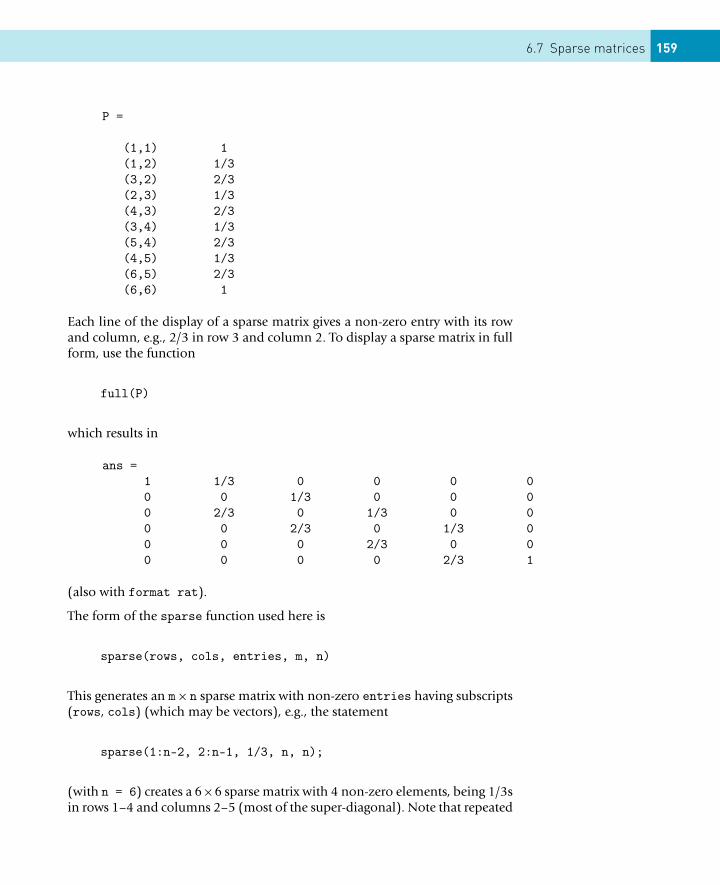
6.7 Sparse matrices 159
P =
(1,1) 1(1,2) 1/3(3,2) 2/3(2,3) 1/3(4,3) 2/3(3,4) 1/3(5,4) 2/3(4,5) 1/3(6,5) 2/3(6,6) 1
Each line of the display of a sparse matrix gives a non-zero entry with its rowand column, e.g., 2/3 in row 3 and column 2. To display a sparse matrix in fullform, use the function
full(P)
which results in
ans =1 1/3 0 0 0 00 0 1/3 0 0 00 2/3 0 1/3 0 00 0 2/3 0 1/3 00 0 0 2/3 0 00 0 0 0 2/3 1
(also with format rat).
The form of the sparse function used here is
sparse(rows, cols, entries, m, n)
This generates an m×n sparse matrix with non-zero entries having subscripts(rows, cols) (which may be vectors), e.g., the statement
sparse(1:n-2, 2:n-1, 1/3, n, n);
(with n = 6) creates a 6×6 sparse matrix with 4 non-zero elements, being 1/3sin rows 1–4 and columns 2–5 (most of the super-diagonal). Note that repeated
160 CHAPTER 6: Matrices and Arrays
use of sparse produces a number of 6 × 6 matrices, which must be addedtogether to give the final form. Sparsity is therefore preserved by operations onsparse matrices. See help for more details of sparse.
It’s quite easy to test the efficiency of sparse matrices. Construct a (full) identitymatrix
a = eye(1000);
Determine the time it takes to compute a^2. Now let us take advantage of thesparseness of a. It is an ideal candidate for being represented as a sparse matrix,since only 1000 of its one million elements are non-zero. It is represented insparse form as
s = sparse(1:1000, 1:1000, 1, 1000, 1000);
Now check the time it takes to find a^2. Use tic and toc to find out how muchfaster is the computation.
The function full(a) returns the full form of the sparse matrix a (withoutchanging the sparse representation of a itself). Conversely, sparse(a) returnsthe sparse form of the full matrix a.
The function spy provides a neat visualization of sparse matrices. Try it on P.Then enlarge P to about 50 × 50, and spy it.
SUMMARY� A matrix is a 2-D array. Elements may be referenced in the conventional
way with two subscripts. Alternatively, one subscript may be used, in whichcase the matrix is ‘unwound’ by columns.
� The colon operator may be used to represent all the rows or columns of amatrix, and also as a single subscript.
� The keyword end refers to the last row or column of a matrix.� Use repmat to duplicate rows or columns of a matrix.� Use the empty array [ ] to delete rows or columns of a matrix.� Arrays may have more than two dimensions. In the case of a 3-D array the
third subscript may be thought of as numbering pages, where each pagecontains a matrix defined by the first two subscripts.
� The matrix operations of multiplication and exponentiation are imple-mented with the matrix operators * and ^.
� The matrix left division operator \ is used for solving systems of linearequations directly. Because the matrix division operators \ and / can some-times produce surprising results with the least squares solution method,
6.7 Exercises 161
you should always compute the residual when solving a system of equa-tions.
� If you work with large matrices with relatively few non-zero entries youshould consider using MATLAB’s sparse matrix facilities.
EXERCISES6.1 Set up any 3×3 matrix a. Write some command-line statements to perform
the following operations on a:(a) interchange columns 2 and 3;(b) add a fourth column (of 0s);(c) insert a row of 1s as the new second row of a (i.e. move the current
second and third rows down);(d) remove the second column.
6.2 Compute the limiting probabilities for the student in Section 6.5 when hestarts at each of the remaining intersections in turn, and confirm that thecloser he starts to the cafe, the more likely he is to end up there.Compute P^50 directly. Can you see the limiting probabilities in the firstrow?
6.3 Solve the equations
2x − y + z = 4
x + y + z = 3
3x − y − z = 1
using the left division operator. Check your solution by computing theresidual. Also compute the determinant (det) and the condition estimator(rcond). What do you conclude?
6.4 This problem, suggested by R.V. Andree, demonstrates ill conditioning(where small changes in the coefficients cause large changes in the solu-tion). Use the left division operator to show that the solution of the system
x + 5.000y = 17.0
1.5x + 7.501y = 25.503
is x = 2, y = 3. Compute the residual.Now change the term on the right-hand side of the second equation to25.501, a change of about one part in 12 000, and find the new solutionand the residual. The solution is completely different. Also try changingthis term to 25.502, 25.504, etc. If the coefficients are subject to experi-mental errors, the solution is clearly meaningless. Use rcond to find thecondition estimator and det to compute the determinant. Do these valuesconfirm ill conditioning?Another way to anticipate ill conditioning is to perform a sensitivity analysison the coefficients: change them all in turn by the same small percentage,and observe what effect this has on the solution.
162 CHAPTER 6: Matrices and Arrays
6.5 Use sparse to represent the Leslie matrix in Section 6.4. Test your repre-sentation by projecting the rabbit population over 24 months.
6.6 If you are familiar with Gauss reduction it is an excellent programming ex-ercise to code a Gauss reduction directly with operations on the rows ofthe augmented coefficient matrix. See if you can write a function
x = mygauss(a, b)
to solve the general system Ax = b. Skillful use of the colon operator in therow operations can reduce the code to a few lines!Test it on A and b with random entries, and on the systems in Section 6.6and Exercise 16.4. Check your solutions with left division.
CONTENTS
Example: Newton’smethod again..... 163
Basic rules ......... 165Subfunctions ......... 170Private functions ... 170P-code files ........... 170Improving M-fileperformance with theprofiler................... 171
Functionhandles................ 171
Command/functionduality.................. 173
Function nameresolution ........... 174
DebuggingM-files ................. 174Debugging a script 174Debugging afunction ................. 176
Recursion ........... 176
Summary ............ 178
Exercises ............ 179
Supplementarymaterial .............. 180
CHAPTER 7
Function M-files
THE OBJECTIVE OF THIS CHAPTER IS TO ENABLE YOU TO:
� Write your own function M-files.
We have already seen that MATLAB has a number of built-in (compiled) func-tions, e.g., sin, sqrt, sum. You can verify that they are built-in by attemptingto type them. Try type sin for example. MATLAB also has some functions inthe form of function M-files, e.g., fzero, why. You can see what’s in them withtype, e.g., type why.
Functions are indispensable when it comes to breaking a problem down intomanageable logical pieces. Hence, MATLAB enables you to create your ownfunction M-files. A function M-file is similar to a script file in that it also hasa .m extension. However, a function M-file differs from a script file in thata function M-file communicates with the MATLAB workspace only throughspecially designated input and output arguments.
We begin this chapter by extending the ideas about implementing function M-files introduced in Chapter 3, Section 3.2.2. We do this by example. We thendeal with the basic rules and the various input/output possibilities availableto you in the development of function M-files. For additional informationand examples type help function in the Command Window and click ondoc function at the bottom of the displayed information.
7.1 EXAMPLE: NEWTON’S METHOD AGAIN
Newton’s method may be used to solve a general equation f (x) = 0 by repeat-ing the assignment
x becomes x − f (x)
f ′(x),
163Essential MATLAB for Engineers and Scientists. DOI:10.1016/B978-0-08-100877-5.00008-6Copyright © 2017 Daniel T. Valentine. Published by Elsevier Ltd. All rights reserved.
164 CHAPTER 7: Function M-files
where f ′(x) (i.e., df/dx) is the first derivative of f (x). The process continuesuntil successive approximations to x are close enough.
Suppose that f (x) = x3 +x−3, i.e., we want to solve the equation x3 +x−3 = 0(another way of stating the problem is to say we want to find the zero of f (x)).We have to be able to differentiate f (x). That’s quite easy here: f ′(x) = 3x2 +1.We could write inline objects for both f (x) and f ′(x), but for this example wewill use function M-files instead.
Use the Editor to create and save (in the current MATLAB directory) the func-tion file f.m as follows:
function y = f(x)y = x^3 + x - 3;
Then create and save another function file df.m:
function y = df(x)y = 3*x^2 + 1;
Now write a separate script file, newtgen.m (in the same directory), which willstop either when the relative error in x is less than 10−8, or after 20 steps, say:
% Newton’s method in general% excludes zero roots!steps = 0; % iteration counterx = input( ’Initial guess: ’ ); % estimate of rootre = 1e-8; % required relative errormyrel = 1;
while myrel > re & (steps < 20)xold = x;x = x - f(x)/df(x);steps = steps + 1;disp( [x f(x)] )myrel = abs((x-xold)/x);
end
if myrel <= redisp( ’Zero found at’ )disp( x )
elsedisp( ’Zero NOT found’ )
end
7.2 Basic rules 165
Note that there are two conditions that will stop the while loop: convergence,or the completion of 20 steps. Otherwise the script could run indefinitely.
Here is a sample run (with format long e), starting with x = 1:
Initial guess: 11.250000000000000e+000 2.031250000000000e-0011.214285714285714e+000 4.737609329445558e-0031.213412175782825e+000 2.779086666571118e-0061.213411662762407e+000 9.583445148564351e-0131.213411662762230e+000 -4.440892098500626e-016
Zero found at1.213411662762230e+000
Note:
� The variable y in the function files f.m and df.m is the output argument. It isa dummy variable, and defines how output will be sent back to the outsideworld.
By the way, you realize of course that you can use your own functions from thecommand line, don’t you? For example,
�f(2)
should return 7 with f.m defined as above.
7.2 BASIC RULES
Try the following more general example, which returns the mean (avg) andstandard deviation (stdev) of the values in the vector x. Although there aretwo MATLAB functions to do this (mean and std), it is useful to have themcombined into one. Write a function file stats.m:
function [avg, stdev] = stats( x ) % function definition line% STATS Mean and standard deviation % H1 line% Returns mean (avg) and standard % Help text% deviation (stdev) of the data in the% vector x, using Matlab functions
avg = mean(x); % function bodystdev = std(x);
Now test it in the Command Window with some random numbers, e.g.,
166 CHAPTER 7: Function M-files
r = rand(100,1);[a, s] = stats(r);
Note the following points about function M-files in general:
� General form of a functionA function M-file name.m has the following general form:
function [ outarg1, outarg2, . . .] = name( inarg1, inarg2, . . .)% comments to be displayed with help...outarg1 = ... ;outarg2 = ... ;...
� function keywordThe function file must start with the keyword function (in the functiondefinition line).
� Input and output argumentsThe input and output arguments (inarg1, outarg1, etc.) are ‘dummy’ vari-ables, and serve only to define the function’s means of communicationwith the workspace. Other variable names may therefore be used in theirplace when the function is called (referenced).You can think of the actual input arguments being copied into the dummyinput arguments when the function is called. So when stats(r) is calledin the above example, the actual input argument r is copied into the inputargument x in the function file. When the function returns (i.e., executionof it is completed) the dummy output arguments avg and stdev in thefunction file are copied into the actual output arguments a and s.
� Multiple output argumentsIf there is more than one output argument, the output arguments must beseparated by commas and enclosed in square brackets in the function defi-nition line, as shown.However, when a function is called with more than one output argument,the actual output arguments may be separated by commas or spaces.If there is only one output argument square brackets are not necessary.
� Naming convention for functionsFunction names must follow the MATLAB rules for variable names.If the filename and the function definition line name are different, the in-ternal name is ignored.
� Help textWhen you type help function_name, MATLAB displays the comment linesthat appear between the function definition line and the first non-comment(executable or blank) line.The first comment line is called the H1 line. The lookfor function searcheson and displays only the H1 line. The H1 lines of all M-files in a direc-
7.2 Basic rules 167
tory are displayed under the Description column of the Desktop CurrentDirectory browser.You can make help text for an entire directory by creating a file with thename Contents.m that resides in the directory. This file must contain onlycomment lines. The contents of Contents.m is displayed with the com-mand
help directory_name
If a directory does not have a Contents.m file, this command displays theH1 line of each M-file in the directory.
� Local variables: scopeAny variables defined inside a function are inaccessible outside the func-tion. Such variables are called local variables—they exist only inside thefunction, which has its own workspace separate from the base workspaceof variables defined in the Command Window.This means that if you use a variable as a loop index, say, inside a function,it will not clash with a variable of the same name in the workspace or inanother function.You can think of the scope of a variable as the range of lines over which thevariable is accessible.
� Global variablesVariables which are defined in the base workspace are not normally acces-sible inside functions, i.e., their scope is restricted to the workspace itself,unless they have been declared global , e.g.,
global PLINK PLONK
If several functions, and possibly the base workspace, all declare particularvariables as global, then they all share single copies of those variables. MAT-LAB recommends that global variables be typed in capital letters, to remindyou that they are global.The function isglobal(A) returns 1 if A is global, and 0 otherwise.The command who global gives a list of global variables.Use clear global to make all variables non-global, or clear PLINK tomake PLINK non-global.
� Persistent variablesA variable in a function may be declared persistent. Local variables nor-mally cease to exist when a function returns. Persistent variables, however,remain in existence between function calls. A persistent variable is initial-ized to the empty array.In the following example, the persistent variable count is used to counthow many times the function test is called:
function test
168 CHAPTER 7: Function M-files
persistent countif isempty(count)
count = 1else
count = count + 1end
Persistent variables remain in memory until the M-file is cleared orchanged, e.g.,
clear test
The function mlock inside an M-file prevents the M-file from being cleared.A locked M-file is unlocked with munlock. The function mislocked indi-cates whether an M-file can be cleared or not.The Help entry on persistent declares confidently: ‘It is an error to declarea variable persistent if a variable with the same name exists in the currentworkspace.’ However, this is definitely not the case at the time of writing(I tried it!).
� Functions that do not return valuesYou might want to write a function that doesn’t return values (such func-tions are called procedures or subroutines in languages like Pascal and Fortran,and void in C++ and Java). In that case you simply omit the output argu-ment(s) and the equal sign in the function definition line. For example, thefollowing function will display n asterisks:
function stars(n)asteriks = char(abs(’*’)*ones(1,n));disp( asteriks )
Go back to Chapter 6 for an explanation of how it works.Write such a function file (stars.m), and test it out, e.g., stars(13) shouldproduce 13 asterisks.
� Vector argumentsIt should come as no surprise that input and output arguments may bevectors, e.g., the following function generates a vector of n random rolls ofa die:
function d = dice( n )d = floor( 6 * rand(1, n) + 1 );
When an output argument is a vector, it is initialized each time the functionis called, any previous elements being cleared. Its size at any moment istherefore determined by the most recent call of the function. For example,suppose the function test.m is defined as
function a = testa(3) = 92;
7.2 Basic rules 169
Then if b is defined in the base workspace as
b =1 2 3 4 5 6
the statement
b = test
results in
b =0 0 92
� How function arguments are passedIf a function changes the value of any of its input arguments, the change isnot reflected in the actual input argument on return to the workspace (un-less the function is called with the same input and output argument—seebelow). For the technically minded, input arguments appear to be passedby value.You might think that passing a large matrix as an input argument by valueis wasteful of memory, and you would be correct. However, the designersof MATLAB were aware of this, and so an input argument is only passed byvalue if a function modifies it (although the modification is not reflectedon return). If a function does not modify an input argument it is passed byreference.
� Simulated pass by referenceA function may be called with the same actual input and output argument.For example, the following function prune.m removes all the zero elementsfrom its input argument:
function y = prune(x)y = x(x ~= 0);
(if you can’t figure out why, refer to Subscripting with logical vectors inChapter 5).You can use it to remove all the zero elements of the vector x as follows:
x = prune(x)
� Checking the number of function argumentsA function may be called with all, some, or none of its input arguments. Ifcalled with no arguments, the parentheses must be omitted. You may notuse more input arguments than appear in its definition.The same applies to output arguments—you may specify all, some, or noneof them when you use the function. If you call a function with no outputarguments, the value of the first one in the definition is returned.
170 CHAPTER 7: Function M-files
There are times when a function may need to know how many input/outputarguments are used on a particular call. In that case, the functions narginand nargout can be used to determine the number of actual input andoutput arguments. For example,
function y = foo(a, b, c);disp( nargin );...
will display the number of input arguments present on each call of foo.� Passing a variable number of arguments
The functions varargin and varargout allow you to call a function withany number of input or output arguments. Since this facility involves pack-ing arguments into a cell array, discussion of it is deferred to Chapter 10.
7.2.1 SubfunctionsA function M-file may contain the code for more than one function. The firstfunction in a file is the primary function, and is the one invoked with the M-filename. Additional functions in the file are called subfunctions, and are visibleonly to the primary function and to other subfunctions.
Each subfunction begins with its own function definition line. Subfunctionsfollow each other in any order after the primary function.
7.2.2 Private functionsA private function is a function residing in a subdirectory with the nameprivate. Private functions are visible only to functions in the parent directory.See Help for more details.
7.2.3 P-code filesThe first time a function is called during a MATLAB session it is parsed (‘com-piled’) into pseudocode and stored in memory to obviate the need for it to beparsed again during the current session. The pseudocode remains in memoryuntil you clear it with clear function_name (see Help for all the possibilitieswith clear).
You can use the pcode function to save the parsed version of an M-file foruse in later MATLAB sessions, or by users from whom you want to hide youralgorithms. For example, the command
pcode stats
parses stats.m and stores the resulting pseudocode in the file named stats.p.
7.3 Function handles 171
MATLAB is very efficient at parsing so producing your own P-code files seldommakes much of a speed difference, except in the case of large GUI applicationswhere many M-files have to be parsed before the application surfaces.
7.2.4 Improving M-file performance with the profilerThe MATLAB Profiler enables you to see where the bottlenecks in your pro-grams are, e.g., which functions are consuming most of the time. With thisinformation you can often redesign programs to be more efficient. To find outmore about this utility open the MATLAB Help documentation via the ‘?’ atthe top of the desktop and type “Profiler” in the search space. You should beat the document titled “The Profiler Utility”.
7.3 FUNCTION HANDLES
Our script file newtgen.m in Section 7.1 solves the equation f (x) = 0, wheref (x) is defined in the function file with the specific name f.m. This is restric-tive because to solve a different equation f.m has to be edited first. To makenewtgen even more general, it can be rewritten as a function M-file itself, witha handle to f.m as an input argument. This process is made possible by thebuilt-in function feval, and the concept of a function handle, which we nowexamine.
Try the following on the command line:
fhandle = @sqrt;feval(fhandle, 9)feval(fhandle, 25)
Can you see that feval(fhandle, x) is the same as sqrt(x)? The statement
fhandle = @sqrt
creates a handle to the function sqrt. The handle provides a way of referringto the function, for example in a list of input arguments to another function.A MATLAB function handle is similar to a pointer in C++, although more gen-eral.
If you have still got a function file f.m defined for f (x) = x3 + x − 3, verify that
feval(@f, 2)
for example, returns the same value as f(2).
172 CHAPTER 7: Function M-files
� In general, the first argument of feval is a handle to the function to beevaluated in terms of the subsequent arguments of feval.
You can use feval inside a function to evaluate another function whose handleis passed as an argument, as we will see now. As an example, we would like torewrite our newtgen script as a function newtfun, to be called as follows:
[x f conv] = newtfun( fh, dfh, x0 )
where fh and dfh are handles for the M-files containing f (x) and f ′(x) respec-tively, and x0 is the initial guess. The outputs are the zero, the function valueat the zero, and an argument conv to indicate whether or not the process hasconverged. The complete M-file newtfun.m is as follows:
function [x, f, conv] = newtfun(fh, dfh, x0)% NEWTON Uses Newton’s method to solve f(x) = 0.% fh is handle to f(x), dfh is handle to f’(x).% Initial guess is x0.% Returns final value of x, f(x), and% conv (1 = convergence, 0 = divergence)
steps = 0; % iteration counterx = x0;re = 1e-8; % required relative errormyrel = 1;
while myrel > re & (steps < 20)xold = x;x = x - feval(fh, x)/feval(dfh, x);steps = steps + 1;disp( [x feval(fh, x)] )myrel = abs((x-xold)/x);
end;
if myrel <= reconv = 1;
elseconv = 0;
end;
f = feval(fh, x);
Try it out. Verify that you can call newtfun with less than three output variables.Also check help newton.
7.4 Command/function duality 173
A function handle gives you more than just a reference to the function. Openthe help document and search for “function handles” to find more informa-tion on this topic.
Functions, such as feval, fplot, newtfun, etc. which take function handlesas arguments are referred to by MATLAB as function functions, as opposed tofunctions which take numeric arrays as arguments.
Use of a function handle to evaluate a function supersedes the earlier use offeval where a string containing the function’s name was passed as an argu-ment.
7.4 COMMAND/FUNCTION DUALITY
In the earliest versions of MATLAB there was a clear distinction between com-mands like
clearsave junk x y zwhos
and functions like
sin(x)plot(x, y)
If commands had any arguments they had to be separated by blanks with nobrackets. Commands altered the environment, but didn’t return results. Newcommands could not be created with M-files.
From Version 4 onwards commands and functions are ‘duals’, in that com-mands are considered to be functions taking string arguments. So
axis off
is the same as
axis( ’off’ )
Other examples are
disp Error!hold(’on’)
This duality makes it possible to generate command arguments with stringmanipulations, and also to create new commands with M-files.
174 CHAPTER 7: Function M-files
7.5 FUNCTION NAME RESOLUTION
Remember that a variable in the workspace can ‘hide’ a built-in function of thesame name, and a built-in function can hide an M-file.
Specifically, when MATLAB encounters a name it resolves it in the followingsteps:
1. Checks if the name is a variable.2. Checks if the name is a subfunction of the calling function.3. Checks if the name is a private function.4. Checks if the name is in the directories specified by MATLAB’s search path.
MATLAB therefore always tries to use a name as a variable first, before trying touse it as a script or function.
7.6 DEBUGGING M-FILES
Run-time errors (as opposed to syntax errors) which occur inside function M-files are often hard to fix, because the function workspace is lost when the errorforces a return to the base workspace. The Editor/Debugger enables you to getinside a function while it is running, to see what’s going wrong.
7.6.1 Debugging a scriptTo see how to debug interactively, let’s first try the script newtgen.m in Sec-tion 7.3. Go through the following steps.
� Open newtgen.m with the MATLAB Editor/Debugger. (Incidentally, haveyou found out that you can run the Editor directly from the command line,e.g., with edit newtgen).You will have noticed that the lines in the Editor window are numbered.You can generate these line numbers from the command line for referencepurposes with the command dbtype:
dbtype newtgen
1 % Newton’s method in general2 % exclude zero roots!34 steps = 0; % iteration counter5 x = input( ’Initial guess: ’ ); % estimate of root6 re = 1e-8; % required relative error7 myrel = 1;89 while myrel > re & (steps < 20)10 xold = x;
7.6 Debugging M-files 175
11 x = x - f(x)/df(x);12 steps = steps + 1;13 disp( [x f(x)] )14 myrel = abs((x-xold)/x);15 end;1617 if myrel <= re18 disp( ’Zero found at’ )19 disp( x )20 else21 disp( ’Zero NOT found’ )22 end;
� To get into Debug mode you need to set a breakpoint just before where youthink the problem might be. Alternatively, if you just want to ‘step through’a script line-by-line, set a breakpoint at the first executable statement. Thecolumn to the right of the line numbers is called the breakpoint alley. Youcan only set breakpoints at executable statements—these are indicated bydashes in the breakpoint alley.Set a breakpoint at line 4 (steps = 0;) by clicking in the breakpoint al-ley. You can remove a breakpoint by clicking on the breakpoint icon, orusing the Editor’s Breakpoints menu (this menu also allows you to specifystopping conditions). You can also set/clear breakpoints on the current linewith the set/clear breakpoint button on the toolbar.
� Having set your breakpoints, run the script in the Editor by clicking the runbutton in the toolbar, or with Debug -> Run (F5).You can also run the script from the command line.
� When the script starts to run, there are two things in particular to notice.First, the symbol K appears to left of the command-line prompt to remindyou that MATLAB is in debug mode.Second, a green arrow appears just to the right of the breakpoint in theEditor. The arrow indicates the next statement which is about to be exe-cuted.
� Now step through the script with Debug -> Step (F10). Note whenline 5 is executed you need to enter the value of x at the commandline.
� When you get to line 11 (x = x - f(x)/df(x);) in this way, use Debug-> Step In (F11) and the Debugger will take you into the functions f.m anddf.m.
� Continue with F10. Note that output appears in the Command Window aseach disp statement is executed.
� There are a number of ways of examining variable values in debugmode:1. Position the cursor to the left of the variable in the Editor. Its current
value appears in a box—this is called a datatip.
176 CHAPTER 7: Function M-files
2. Type the name of the variable in the Command Window.3. Use the Array Editor: open the Workspace browser and double-click a
variable. If you arrange your windows carefully you can watch the valueof a variable change in the Array Editor while you step through a pro-gram.Note that you can view variables only in the current workspace. TheEditor has a Stack field to the right of the toolbar where you canselect the workspace. For example, if you have stepped into f.m thecurrent workspace is shown as f. At this point you can view vari-ables in the newtgen workspace by selecting newtgen in the Stackfield.
You can use the Array Editor or the command line to change the value ofa variable. You can then continue to see how the script performs with thenew value.
� Another useful debugging feature is Debug -> Go Until Cursor. This en-ables you to continue running the script to the line where you’ve positionedthe cursor.
� To quit debugging click the exit debug mode button in the Editor/Debuggertoolbar, or select Debug -> Exit Debug Mode.If you forget to quit debugging you won’t be able to get rid of the K prompton the command line!
7.6.2 Debugging a functionYou can’t run a function directly in the Editor/Debugger—you have to seta breakpoint in the function and run it from the command line. Let’s usenewtfun.m as an example.
� Open newtfun.m in the Editor/Debugger.� Set a breakpoint at line 8 (steps = 0;).� In the Command Window set up function handles for f and df and call
newtfun:
fhand = @f;dfhand = @df;[x f conv] = newtfun(fhand, dfhand, 10)
� Note that MATLAB goes into debug mode and takes you to the breakpointin newtfun. Now you can continue debugging as before.
Debugging may also be done from the command line with the debug func-tions. See help debug.
7.7 RECURSION
Many (mathematical) functions are defined recursively, i.e., in terms of simplercases of themselves, e.g., the factorial function may be defined recursively as
7.7 Recursion 177
n! = n × (n − 1)!as long as 1! is defined as 1. MATLAB allows functions to call themselves; thisprocess is called recursion. The factorial function may be written recursively inan M-file fact.m like this:
function y = fact(n)% FACT Recursive definition of n!
if n > 1y = n * fact(n-1);
elsey = 1;
end;
Recursive functions are usually written in this way: an if statement handlesthe general recursive definition; the else part handles the special case (n = 1).
Although recursion appears deceptively simple, it is an advanced topic, as thefollowing experiment demonstrates. Insert the statement disp(n) into the def-inition of fact immediately above the if statement, and run fact(5) from thecommand line. The effect is what you might expect: the integers 5 to 1 in de-scending order. Now move disp(n) to below the if statement, and see whathappens. The result is the integers 1 to 5 in ascending order now, which is rathersurprising.
In the first case, the value of n is displayed each time fact is called, and theoutput is obvious enough. However, there is the world of difference betweena recursive function being called, and executed. In the second case, the dispstatement is only executed after the if has finished executing. And when isthat exactly? Well, when the initial call to fact takes place, n has the value 5,so the first statement in the if is invoked. However, the value of fact(4) isnot known at this stage, so a copy is made of all the statements in the functionwhich will need to be executed once the value of fact(4) is known. The refer-ence to fact(4) makes fact call itself, this time with a value of 4 for n. Again,the first statement in the if is invoked, and MATLAB discovers that it doesn’tknow the value of fact(3) this time. So another (different) copy is made ofall the statements that will have to be executed once the value of fact(3) isknown. And so each time fact is called, separate copies are made of all thestatements yet to be executed. Finally, MATLAB joyfully finds a value of n (1) forwhich it actually knows the value of fact, so it can at last begin to execute (inreverse order) the pile of statements which have been damming up inside thememory.
This discussion illustrates the point that recursion should be treated with re-spect. While it is perfectly in order to use it in an example like this, it can chewup huge amounts of computer memory and time.
178 CHAPTER 7: Function M-files
SUMMARY� Good structured programming requires real problem-solving programs to
be broken down into function M-files.� The name of a function in the function definition line should be the same
as the name of the M-file under which it is saved. The M-file must have theextension .m.
� A function may have input and output arguments, which are usually itsonly way of communicating with the workspace. Input/output argumentsare dummy variables (placeholders).
� Comment lines up to the first non-comment line in a function are displayedwhen help is requested for the function.
� Variables defined inside a function are local variables and are inaccessibleoutside the function.
� Variables in the workspace are inaccessible inside a function unless theyhave been declared global.
� A function does not have to have any output arguments.� Input arguments have the appearance of being passed by value to a func-
tion. This means that changes made to an input argument inside a functionare not reflected in the actual input argument when the function returns.
� A function may be called with fewer than its full number of input/outputarguments.
� The functions nargin and nargout indicate how many input and outputarguments are used on a particular function call.
� Variables declared persistent inside a function retain their values betweencalls to the function.
� Subfunctions in an M-file are accessible only to the primary function andto other subfunctions in the same M-file.
� Private functions are functions residing in a sub-directory named privateand are accessible only to functions in the parent directory.
� Functions may be parsed (compiled) with the pcode function. The resultingcode has the extension .p and is called a P-code file.
� The Profiler enables you to find out where your programs spend most oftheir time.
� A handle for a function is created with @.A function may be represented by its handle. In particular the handle maybe passed as an argument to another function.
� feval evaluates a function whose handle is passed to it as an argument.� MATLAB first tries to use a name as a variable, then as a built-in function,
and finally as one of the various types of function.� Command/function duality means that new commands can be created
with function M-files, and that command arguments may be generated withstring manipulations.
� The Editor/Debugger enables you to work through a script or function line-by-line in debug mode, examining and changing variables on the way.
� A function may call itself. This feature is called recursion.
7.7 Exercises 179
EXERCISES7.1 Change the function stars of Section 7.2 to a function pretty so that it
will draw a line of any specified character. The character to be used mustbe passed as an additional input (string) argument, e.g., pretty(6, ’$’)should draw six dollar symbols.
7.2 Write a script newquot.m which uses the Newton quotient [f (x + h) −f (x)]/h to estimate the first derivative of f (x) = x3 at x = 1, using suc-cessively smaller values of h: 1, 10−1, 10−2, etc. Use a function M-file forf (x).Rewrite newquot as a function M-file able to take a handle for f (x) as aninput argument.
7.3 Write and test a function double(x) which doubles its input argument,i.e., the statement x = double(x) should double the value in x.
7.4 Write and test a function swop(x, y) which will exchange the values ofits two input arguments.
7.5 Write your own MATLAB function to compute the exponential functiondirectly from the Taylor series:
ex = 1 + x + x2
2! + x3
3! + . . .
The series should end when the last term is less than 10−6. Test your func-tion against the built-in function exp, but be careful not to make x toolarge—this could cause rounding error.
7.6 If a random variable X is distributed normally with zero mean and unitstandard deviation, the probability that 0 ≤ X ≤ x is given by the standardnormal function �(x). This is usually looked up in tables, but it may beapproximated as follows:
�(x) = 0.5 − r(at + bt2 + ct3),
where a = 0.4361836, b = −0.1201676, c = 0.937298, r = exp(−0.5x2)/√
2π ,and t = 1/(1 + 0.3326x).Write a function to compute �(x), and use it in a program to write out itsvalues for 0 ≤ x ≤ 4 in steps of 0.1. Check: �(1) = 0.3413.
7.7 Write a function
function [x1, x2, flag] = quad( a, b, c )
which computes the roots of the quadratic equation ax2 + bx + c = 0. Theinput arguments a, b and c (which may take any values) are the coefficientsof the quadratic, and x1, x2 are the two roots (if they exist), which maybe equal. See Figure 3.3 in Chapter 3 for the structure plan. The outputargument flag must return the following values, according to the numberand type of roots:0: no solution (a = b = 0, c �= 0);
180 CHAPTER 7: Function M-files
1: one real root (a = 0, b �= 0, so the root is −c/b);2: two real or complex roots (which could be equal if they are real);99: any x is a solution (a = b = c = 0).Test your function on the data in Exercise 3.5.
7.8 The Fibonacci numbers are generated by the sequence
1,1,2,3,5,8,13, . . .
Can you work out what the next term is? Write a recursive function f(n)to compute the Fibonacci numbers F0 to F20, using the relationship
Fn = Fn−1 + Fn−2,
given that F0 = F1 = 1.7.9 The first three Legendre polynomials are P0(x) = 1, P1(x) = x, and
P2(x) = (3x2 − 1)/2. There is a general recurrence formula for Legendrepolynomials, by which they are defined recursively:
(n + 1)Pn+1(x) − (2n + 1)xPn(x) + nPn−1(x) = 0.
Define a recursive function p(n,x) to generate Legendre polynomials,given the form of P0 and P1. Use your function to compute p(2,x) fora few values of x, and compare your results with those using the analyticform of P2(x) given above.
APPENDIX 7.A SUPPLEMENTARY MATERIAL
Supplementary material related to this chapter can be found online at http://dx.doi.org/10.1016/B978-0-08-100877-5.00008-6.
CONTENTS
Determinaterepetition withfor........................ 181Binomialcoefficient .............. 181Update processes.. 182Nested fors ........... 184
Indeterminaterepetition withwhile ................... 184A guessing game ... 184The whilestatement .............. 185Doubling time of aninvestment............. 185Prime numbers ..... 187Projectiletrajectory ............... 188break and continue190Menus.................... 190
Summary ............ 191
Exercises ............ 192
CHAPTER 8
Loops
THE OBJECTIVES OF THIS CHAPTER ARE TO ENABLE YOUTO LEARN TO:
� Program (or code) determinate loops with for.� Program (or code) indeterminate loops with while.
In Chapter 2 we introduced the powerful for statement, which is used to repeata block of statements a fixed number of times. This type of structure, where thenumber of repetitions must be determined in advance, is sometimes calleddeterminate repetition. However, it often happens that the condition to end aloop is only satisfied during the execution of the loop itself . Such a structure iscalled indeterminate. We begin with a discussion of determinate repetition.
8.1 DETERMINATE REPETITION WITH for
8.1.1 Binomial coefficientThe binomial coefficient is widely used in mathematics and statistics. It is definedas the number of ways of choosing r objects out of n without regard to order,and is given by(
n
r
)= n!
r!(n − r)! . (8.1)
If this form is used, the factorials can get very big, causing an overflow. But alittle thought reveals we can simplify Equation (8.1) as follows:(
n
r
)= n(n − 1)(n − 2) · · · (n − r + 1)
r! , (8.2)
e.g.,(
103
)= 10!
3! × 7! = 10 × 9 × 8
1 × 2 × 3.
Using Equation (8.2) is computationally much more efficient:181
Essential MATLAB for Engineers and Scientists. DOI:10.1016/B978-0-08-100877-5.00009-8Copyright © 2017 Daniel T. Valentine. Published by Elsevier Ltd. All rights reserved.
182 CHAPTER 8: Loops
ncr = 1;n = ...r = ...
for k = 1:rncr = ncr * (n - k + 1) / k;
end
disp( ncr )
The binomial coefficient is sometimes pronounced ‘n-see-r’. Work through theprogram by hand with some sample values.
8.1.2 Update processesMany problems in science and engineering involve modeling a process wherethe main variable is repeatedly updated over a period of time. Here is an ex-ample of such an update process.
A can of orange juice at temperature 25 ◦C is placed in a fridge, where theambient temperature F is 10 ◦C. We want to find out how the temperature ofthe orange juice changes over a period of time. A standard way of approachingthis type of problem is to break the time period up into a number of smallsteps, each of length dt. If Ti is the temperature at the beginning of step i, wecan use the following model to get Ti+1 from Ti :
Ti+1 = Ti − K dt (Ti − F), (8.3)
where K is a constant parameter depending on the insulating properties of thecan, and the thermal properties of orange juice. Assume that units are chosenso that time is in minutes.
The following script implements this scheme. To make the solution more gen-eral, take the starting time as a, and the end time as b. If dt is very small, it willbe inconvenient to have output displayed after every step, so the script also asksyou for the output interval opint. This is the time (in minutes) between succes-sive rows of output. It checks that this interval is an integer multiple of dt .Try the script with some sample values, e.g., dt = 0.2 minutes and opint = 5minutes (these are the values used for the output below).
K = 0.05;F = 10;a = 0; % start timeb = 100; % end timetime = a; % initialize timeT = 25; % initialize temperatureload train % prepare to blow the whistle
8.1 Determinate repetition with for 183
dt = input( ’dt: ’ );opint = input( ’output interval (minutes): ’ );if opint/dt ~= fix(opint/dt)
sound(y, Fs) % blow the whistle!disp( ’output interval is not a multiple of dt!’ );break
end
clcformat bankdisp( ’ Time Temperature’ );disp( [time T] ) % display initial values
for time = a+dt : dt : bT = T - K * dt * (T - F);if abs(rem(time, opint)) < 1e-6 % practically zero!
disp( [time T] )end
end
Output:
Time Temperature0 25.00
5.00 21.67...
95.00 10.13100.00 10.10
Note:
1. The function rem is used to display the results every opint minutes: whentime is an integer multiple of opint its remainder when divided by opintshould be zero. However, due to rounding error, the remainder is not alwaysexactly zero. It is therefore better to test whether its absolute value is lessthan some very small value. (Rounding error is discussed in Chapter 11.)
2. While this is probably the most obvious way of writing the script, we cannoteasily plot the graph of temperature against time this way, since time and Tare scalars which are repeatedly updated. To plot the graph they both needto be vectors (see Chapter 9).
3. Note how sound is implemented. See help audio for other interestingsounds supplied by MATLAB.
4. In case you are wondering how I got the headings in the right place, I’ll letyou into the secret. Run the script without a heading but with the numer-ical output as you want it. Then simply paste the disp statement with the
184 CHAPTER 8: Loops
headings into the command window and edit it until the headings fall inthe right place. Paste the final version of the disp statement into the script.
5. Note the use of break to stop the script prematurely if the user gives badinput. See below for more general use of break.
8.1.3 Nested forsAs we saw in Chapter 2 (Vectorizing nested fors), for loops can be nestedinside each other. The main point to note is that the index of the inner formoves faster.
8.2 INDETERMINATE REPETITION WITH while
Determinate loops all have in common the fact that you can work out in prin-ciple exactly how many repetitions are required before the loop starts. But in thenext example, there is no way in principle of working out the number of repeats,so a different structure is needed.
8.2.1 A guessing gameThe problem is easy to state. MATLAB ‘thinks’ of an integer between 1 and10 (i.e., generates one at random). You have to guess it. If your guess is toohigh or too low, the script must say so. If your guess is correct, a message ofcongratulations must be displayed.
A little more thought is required here, so a structure plan might be helpful:
1. Generate random integer2. Ask user for guess3. While guess is wrong:
If guess is too lowTell her it is too low
OtherwiseTell her it is too high
Ask user for new guess4. Polite congratulations5. Stop.
Here is the script:
matnum = floor(10 * rand + 1);guess = input( ’Your guess please: ’ );load splat
while guess ~= matnumsound(y, Fs)
if guess > matnum
8.2 Indeterminate repetition with while 185
disp( ’Too high’ )else
disp( ’Too low’ )end;
guess = input( ’Your next guess please: ’ );end
disp( ’At last!’ )load handelsound(y, Fs) % hallelujah!
Try it out a few times. Note that the while loop repeats as long as matnum is notequal to guess. There is no way in principle of knowing how many loops willbe needed before the user guesses correctly. The problem is truly indeterminate.
Note that guess has to be input in two places: firstly to get the while loopgoing, and secondly during the execution of the while.
8.2.2 The while statementIn general the while statement looks like this:
while conditionstatementsend
The while construct repeats statements WHILE its condition remains true. Thecondition therefore is the condition to repeat once again. The condition istested each time BEFORE statements are repeated. Since the condition is evalu-ated before statements are executed, it is possible to arrange for statements not tobe executed at all under certain circumstances. Clearly, condition must dependon statements in some way, otherwise the loop will never end.
Recall that a vector condition is considered true only if all its elements are non-zero.
The command-line form of while is:
while condition statements, end
8.2.3 Doubling time of an investmentSuppose we have invested some money which draws 10% interest per year,compounded. We would like to know how long it takes for the investment todouble. More specifically, we want a statement of the account each year, untilthe balance has doubled. The English statement of the problem hints heavilythat we should use an indeterminate loop with the following structure plan:
186 CHAPTER 8: Loops
1. Initialize balance, year, interest rate2. Display headings3. Repeat
Update balance according to interest rateDisplay year, balance
until balance exceeds twice original balance4. Stop.
A program to implement this plan would be
a = 1000;r = 0.1;bal = a;year = 0;disp( ’Year Balance’ )
while bal < 2 * abal = bal + r * bal;year = year + 1;disp( [year bal] )
end
Note that the more natural phrase in the structure plan ‘until balance exceedstwice original balance’ must be coded as
while bal < 2 * a ...
This condition is checked each time before another loop is made. Repetitionoccurs only if the condition is true. Here’s some output (for an opening balanceof $1000):
Year Balance
1 1100.002 1210.003 1331.004 1464.105 1610.516 1771.567 1948.728 2143.59
Note that when the last loop has been completed, the condition to repeat isfalse for the first time, since the new balance ($2143.59) is more than $2000.
8.2 Indeterminate repetition with while 187
Note also that a determinate for loop cannot be used here because we don’tknow how many loops are going to be needed until after the script has run(although in this particular example perhaps you could work out in advancehow many repeats are needed?).
If you want to write the new balance only while it is less than $2000, all thathas to be done is to move the statement
disp( [year bal] )
until it is the first statement in the while loop. Note that the initial balance of$1000 is displayed now.
8.2.4 Prime numbersMany people are obsessed with prime numbers, and most books on program-ming have to include an algorithm to test if a given number is prime. So here’smine.
A number is prime if it is not an exact multiple of any other number exceptitself and 1, i.e., if it has no factors except itself and 1. The easiest plan ofattack then is as follows. Suppose P is the number to be tested. See if anynumbers N can be found that divide into P without remainder. If there arenone, P is prime. Which numbers N should we try? Well, we can speed thingsup by restricting P to odd numbers, so we only have to try odd divisors N .When do we stop testing? When N = P ? No, we can stop a lot sooner. In fact,we can stop once N reaches
√P , since if there is a factor greater than
√P there
must be a corresponding one less than√
P , which we would have found. Andwhere do we start? Well, since N = 1 will be a factor of any P , we should startat N = 3. The structure plan is as follows:
1. Input P
2. Initialize N to 33. Find remainder R when P is divided by N
4. While R �= 0 and N <√
P repeat:Increase N by 2Find R when P is divided by N
5. If R �= 0 thenP is prime
ElseP is not prime
6. Stop.
Note that there may be no repeats—R might be zero the first time. Note alsothat there are two conditions under which the loop may stop. Consequently,an if is required after completion of the loop to determine which conditionstopped it.
188 CHAPTER 8: Loops
See if you can write the script. Then try it out on the following numbers:4 058 879 (not prime), 193 707 721 (prime) and 2 147 483 647 (prime). Ifsuch things interest you, the largest known prime number at the time of writingwas 26 972 593 − 1 (discovered in June 1999). It has 2 098 960 digits and wouldoccupy about 70 pages if it was printed in a newspaper. Obviously our algo-rithm cannot test such a large number, since it’s unimaginably greater thanthe largest number which can be represented by MATLAB. Ways of testing suchhuge numbers for primality are described in D.E. Knuth, The Art of ComputerProgramming. Volume 2: Seminumerical Algorithms (Addison-Wesley, 1981). Thisparticular whopper was found by the GIMPS (Great Internet Mersenne PrimeSearch). See http://www.utm.edu/research/primes/largest.html for more infor-mation on the largest known primes.
8.2.5 Projectile trajectoryIn Chapter 3 we considered the flight of a projectile, given the usual equationsof motion (assuming no air resistance). We would like to know now when andwhere it will hit the ground. Although this problem can be solved with a deter-minate loop (if you know enough applied mathematics), it is of interest also tosee how to solve it with an indeterminate while loop. The idea is to calculatethe trajectory repeatedly with increasing time, while the vertical displacement(y) remains positive. Here’s the script:
dt = 0.1;g = 9.8;u = 60;ang = input( ’Launch angle in degrees: ’ );ang = ang * pi / 180; % convert to radiansx = 0; y = 0; t = 0; % for startersmore(15)
while y >= 0disp( [t x y] );t = t + dt;y = u * sin(ang) * t - g * t^2 / 2;x = u * cos(ang) * t;
end
The command more(n) gives you n lines of output before pausing. This iscalled paging. To get another single line of output press Enter. To get the nextpage of n lines press the spacebar. To quit the script press q.
Try the script for some different launch angles. Can you find the launch anglewhich gives the maximum horizontal range (x)? What launch angle keeps it inthe air for the longest time?
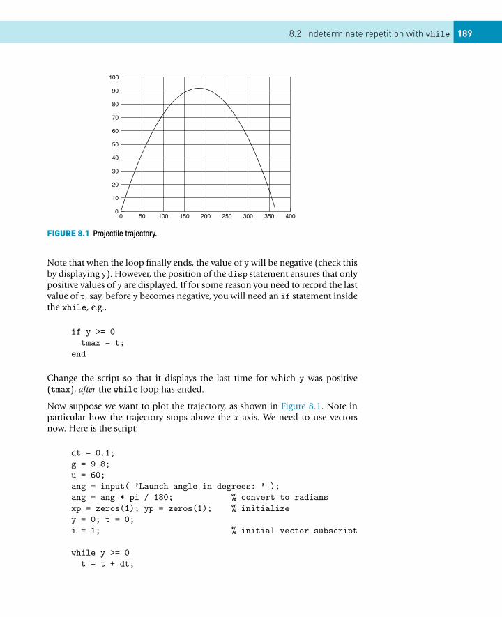
8.2 Indeterminate repetition with while 189
FIGURE 8.1 Projectile trajectory.
Note that when the loop finally ends, the value of y will be negative (check thisby displaying y). However, the position of the disp statement ensures that onlypositive values of y are displayed. If for some reason you need to record the lastvalue of t, say, before y becomes negative, you will need an if statement insidethe while, e.g.,
if y >= 0tmax = t;
end
Change the script so that it displays the last time for which y was positive(tmax), after the while loop has ended.
Now suppose we want to plot the trajectory, as shown in Figure 8.1. Note inparticular how the trajectory stops above the x-axis. We need to use vectorsnow. Here is the script:
dt = 0.1;g = 9.8;u = 60;ang = input( ’Launch angle in degrees: ’ );ang = ang * pi / 180; % convert to radiansxp = zeros(1); yp = zeros(1); % initializey = 0; t = 0;i = 1; % initial vector subscript
while y >= 0t = t + dt;
190 CHAPTER 8: Loops
i = i + 1;y = u * sin(ang) * t - g * t^2 / 2;if y >= 0
xp(i) = u * cos(ang) * t;yp(i) = y;
endend
plot(xp, yp),grid
Note that the function zeros is used to initialize the vectors. This also clearsany vector of the same name hanging around in the workspace from previousruns.
Note also the use of an if inside the while loop to ensure that only co-ordinates of points above the ground are added to the vectors xp and yp.
If you want the last point above the ground to be closer to the ground, try asmaller value of dt, e.g., 0.01.
8.2.6 break and continueAny loop structure you are likely to encounter in scientific programming canbe coded with either ‘pure’ for or while loops, as illustrated by the examplesin this chapter. However, as a concession to intellectual laziness I feel obligedto mention in passing the break and continue statements.
If there are a number of different conditions to stop a while loop you maybe tempted to use a for with the number of repetitions set to some acceptedcut-off value (or even Inf) but enclosing if statements which break out of thefor when the various conditions are met. Why is this not regarded as the bestprogramming style? The reason is simply that when you read the code monthslater you will have to wade through the whole loop to find all the conditionsto end it, rather than see them all paraded at the start of the loop in the whileclause.
If you are going to insist on using break you will have to look it up in help foryourself!
The continue statement is somewhat less virulent than break . . .
8.2.7 MenusTry the following program, which sets up a menu window, as in Figure 8.2:
k = 0;
while k ~= 3
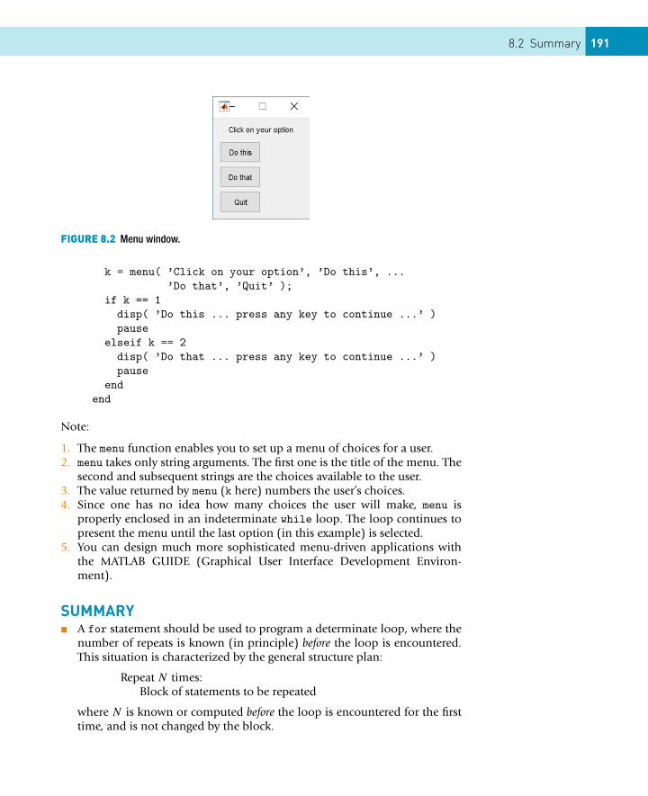
8.2 Summary 191
FIGURE 8.2 Menu window.
k = menu( ’Click on your option’, ’Do this’, ...’Do that’, ’Quit’ );
if k == 1disp( ’Do this ... press any key to continue ...’ )pause
elseif k == 2disp( ’Do that ... press any key to continue ...’ )pause
endend
Note:
1. The menu function enables you to set up a menu of choices for a user.2. menu takes only string arguments. The first one is the title of the menu. The
second and subsequent strings are the choices available to the user.3. The value returned by menu (k here) numbers the user’s choices.4. Since one has no idea how many choices the user will make, menu is
properly enclosed in an indeterminate while loop. The loop continues topresent the menu until the last option (in this example) is selected.
5. You can design much more sophisticated menu-driven applications withthe MATLAB GUIDE (Graphical User Interface Development Environ-ment).
SUMMARY� A for statement should be used to program a determinate loop, where the
number of repeats is known (in principle) before the loop is encountered.This situation is characterized by the general structure plan:
Repeat N times:Block of statements to be repeated
where N is known or computed before the loop is encountered for the firsttime, and is not changed by the block.
192 CHAPTER 8: Loops
� A while statement should be used to program an indeterminate repeatstructure, where the exact number of repeats is not known in advance. An-other way of saying this is that these statements should be used wheneverthe truth value of the condition for repeating is changed in the body of theloop. This situation is characterized by the following structure plan:
While condition is true repeat:statements to be repeated (reset truth value of condition).
Note that condition is the condition to repeat.� The statements in a while construct may sometimes never be executed.� Loops may be nested to any depth.� The menu statement inside a while loop may be used to present a user with
a menu of choices.
EXERCISES8.1 A person deposits $1000 in a bank. Interest is compounded monthly
at the rate of 1% per month. Write a program which will compute themonthly balance, but write it only annually for 10 years (use nestedfor loops, with the outer loop for 10 years, and the inner loop for 12months). Note that after 10 years, the balance is $3300.39, whereas ifinterest had been compounded annually at the rate of 12% per year thebalance would only have been $3105.85.See if you can vectorize your solution.
8.2 There are many formulae for computing π (the ratio of a circle’s circum-ference to its diameter). The simplest is
π
4= 1 − 1/3 + 1/5 − 1/7 + 1/9 − . . . (8.4)
which comes from putting x = 1 in the series
arctanx = x − x3
3+ x5
5− x7
7+ x9
9− . . . (8.5)
(a) Write a program to compute π using Equation (8.4). Use as manyterms in the series as your computer will reasonably allow (startmodestly, with 100 terms, say, and re-run your program with moreand more each time). You should find that the series converges veryslowly, i.e. it takes a lot of terms to get fairly close to π .
(b) Rearranging the series speeds up the convergence:
π
8= 1
1 × 3+ 1
5 × 7+ 1
9 × 11. . .
Write a program to compute π using this series instead. You shouldfind that you need fewer terms to reach the same level of accuracythat you got in (a).
8.2 Exercises 193
(c) One of the fastest series for π is
π
4= 6 arctan
1
8+ 2 arctan
1
57+ arctan
1
239.
Use this formula to compute π . Don’t use the MATLAB function atanto compute the arctangents, since that would be cheating. Rather useEquation (8.5).
(d) Can you vectorize any of your solutions (if you haven’t already)?8.3 The following method of computing π is due to Archimedes:
1. Let A = 1 and N = 62. Repeat 10 times, say:
Replace N by 2N
Replace A by [2 − √(4 − A2)]1/2
Let L = NA/2Let U = L/
√1 − A2/2
Let P = (U + L)/2 (estimate of π)Let E = (U − L)/2 (estimate of error)Print N , P , E
3. Stop.Write a program to implement the algorithm.
8.4 Write a program to compute a table of the function
f (x) = x sin
[π(1 + 20x)
2
]
over the (closed) interval [−1, 1] using increments in x of (a) 0.2, (b)0.1 and (c) 0.01.Use your tables to sketch graphs of f (x) for the three cases (by hand),and observe that the tables for (a) and (b) give totally the wrong pictureof f (x).Get your program to draw the graph of f (x) for the three cases, super-imposed.
8.5 The transcendental number e (2.71828182845904 . . . ) can be shown tobe the limit of
(1 + x)1/x
as x tends to zero (from above). Write a program which shows how thisexpression converges to e as x gets closer and closer to zero.
8.6 A square wave of period T may be defined by the function
f (t) ={
1 (0 < t < T )
−1 (−T < t < 0).
The Fourier series for f (t) is given by
F(t) = 4
π
∞∑k=0
1
2k + 1sin
[(2k + 1)πt
T
].
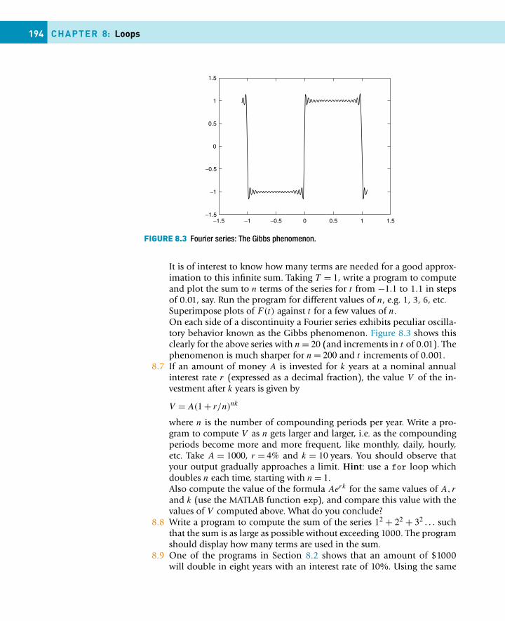
194 CHAPTER 8: Loops
FIGURE 8.3 Fourier series: The Gibbs phenomenon.
It is of interest to know how many terms are needed for a good approx-imation to this infinite sum. Taking T = 1, write a program to computeand plot the sum to n terms of the series for t from −1.1 to 1.1 in stepsof 0.01, say. Run the program for different values of n, e.g. 1, 3, 6, etc.Superimpose plots of F(t) against t for a few values of n.On each side of a discontinuity a Fourier series exhibits peculiar oscilla-tory behavior known as the Gibbs phenomenon. Figure 8.3 shows thisclearly for the above series with n = 20 (and increments in t of 0.01). Thephenomenon is much sharper for n = 200 and t increments of 0.001.
8.7 If an amount of money A is invested for k years at a nominal annualinterest rate r (expressed as a decimal fraction), the value V of the in-vestment after k years is given by
V = A(1 + r/n)nk
where n is the number of compounding periods per year. Write a pro-gram to compute V as n gets larger and larger, i.e. as the compoundingperiods become more and more frequent, like monthly, daily, hourly,etc. Take A = 1000, r = 4% and k = 10 years. You should observe thatyour output gradually approaches a limit. Hint: use a for loop whichdoubles n each time, starting with n = 1.Also compute the value of the formula Aerk for the same values of A, r
and k (use the MATLAB function exp), and compare this value with thevalues of V computed above. What do you conclude?
8.8 Write a program to compute the sum of the series 12 + 22 + 32 . . . suchthat the sum is as large as possible without exceeding 1000. The programshould display how many terms are used in the sum.
8.9 One of the programs in Section 8.2 shows that an amount of $1000will double in eight years with an interest rate of 10%. Using the same
8.2 Exercises 195
interest rate, run the program with initial balances of $500, $2000 and$10000 (say) to see how long they all take to double. The results maysurprise you.
8.10 Write a program to implement the structure plan of Exercise 3.2.8.11 Use the Taylor series
cosx = 1 − x2
2! + x4
4! − x6
6! + . . .
to write a program to compute cosx correct to four decimal places (x isin radians). See how many terms are needed to get 4-figure agreementwith the MATLAB function cos. Don’t make x too large; that could causerounding error.
8.12 A student borrows $10 000 to buy a used car. Interest on her loan is com-pounded at the rate of 2% per month while the outstanding balance ofthe loan is more than $5000, and at 1% per month otherwise. She paysback $300 every month, except for the last month, when the repaymentmust be less than $300. She pays at the end of the month, after the inter-est on the balance has been compounded. The first repayment is madeone month after the loan is paid out. Write a program which displays amonthly statement of the balance (after the monthly payment has beenmade), the final payment, and the month of the final payment.
8.13 A projectile, the equations of motion of which are given in Chapter 3, islaunched from the point O with an initial velocity of 60 m/s at an angleof 50◦ to the horizontal. Write a program which computes and displaysthe time in the air, and horizontal and vertical displacement from thepoint O every 0.5 s, as long as the projectile remains above a horizontalplane through O.
8.14 When a resistor (R), capacitor (C) and battery (V ) are connected inseries, a charge Q builds up on the capacitor according to the formula
Q(t) = CV (1 − e−t/RC)
if there is no charge on the capacitor at time t = 0. The problem is tomonitor the charge on the capacitor every 0.1 s in order to detect whenit reaches a level of 8 units of charge, given that V = 9, R = 4 and C = 1.Write a program which displays the time and charge every 0.1 secondsuntil the charge first exceeds 8 units (i.e. the last charge displayed mustexceed 8). Once you have done this, rewrite the program to display thecharge only while it is strictly less than 8 units.
8.15 Adapt your program for the prime number algorithm in Section 8.2 tofind all the prime factors of a given number (even or odd).
CONTENTS
Basic 2-Dgraphs ................. 197Labels.................... 198Multiple plots on thesame axes ............. 199Line styles, markersand color ............... 200Axis limits.............. 200axes and axis?......... 201Multiple plots in afigure: subplot ...... 202figure, clf and cla203Graphical input ...... 203Logarithmic plots .. 203Polar plots ............. 204Plotting rapidlychanging mathematicalfunctions: fplot .... 205The property editor 206
3-D plots ............. 206plot3 ..................... 206Animated 3-D plotswith comet3 ............ 207Mesh surfaces ....... 207Contour plots......... 209Cropping a surface withNaNs ........................ 211Visualizing vectorfields....................... 211
CHAPTER 9
MATLAB Graphics
THE OBJECTIVE OF THIS CHAPTER IS TO INTRODUCE YOUTO:
� MATLAB’s high-level 2-D and 3-D plotting facilities� Handle Graphics� Editing plots� Animation� Saving and exporting graphs� Color, lighting and the camera
A picture, it is said, is worth a thousand words. MATLAB has a powerful graph-ics system for presenting and visualizing data, which is reasonably easy to use.(Most of the figures in this book have been generated by MATLAB.)
This chapter introduces MATLAB’s high-level 2-D and 3-D plotting facilities.Low-level features, such as handle graphics, are discussed later in this chapter.
It should be stressed that the treatment of graphics in this chapter is of ne-cessity brief, and intended to give you a glimpse of the richness and power ofMATLAB graphics. For the full treatment, you should consult help on the func-tions mentioned in this chapter, as well as the comprehensive list of graphicsfunctions in Help document which you open up by clicking the ‘?’ and typinggraphics in the search tool.
9.1 BASIC 2-D GRAPHS
Graphs (in 2-D) are drawn with the plot statement. In its simplest form, ittakes a single vector argument as in plot(y). In this case the elements of y areplotted against their indexes, e.g., plot(rand(1, 20)) plots 20 random num-bers against the integers 1–20, joining successive points with straight lines, asin Figure 9.1. If y is a matrix, its columns are plotted against element indexes.
197Essential MATLAB for Engineers and Scientists. DOI:10.1016/B978-0-08-100877-5.00010-4Copyright © 2017 Daniel T. Valentine. Published by Elsevier Ltd. All rights reserved.
Visualization ofmatrices ................ 212Rotation of 3-Dgraphs ................... 213
Handle graphics 214Getting handles ..... 214Graphics objectproperties and how tochange them ......... 215A vector of handles 217Graphics objectcreation functions . 218Parenting............... 218Positioning figures 219
Editing plots ....... 220Plot edit mode ....... 220Property Editor ...... 221
Animation ........... 222Animation with HandleGraphics ................ 222
Color etc. ............ 225Colormaps ............. 225Color of surfaceplots....................... 226Truecolor ............... 228
Lighting andcamera ................ 228
Saving, printing andexportinggraphs ................. 229Saving and openingfigure files ............. 229Printing a graph .... 229Exporting a graph.. 229
Summary ............ 230
Exercises ............ 231
198 CHAPTER 9: MATLAB Graphics
FIGURE 9.1 Examples of plot.
Axes are automatically scaled and drawn to include the minimum and maxi-mum data points.
Probably the most common form of plot is plot(x, y) where x and y arevectors of the same length, e.g.,
x = 0:pi/40:4*pi;plot(x, sin(x))
In this case, the co-ordinates of the ith point are xi , yi . This form of plot hasbeen used widely in earlier chapters.
Straight-line graphs are drawn by giving the x and y co-ordinates of the end-points in two vectors. For example, to draw a line between the point withcartesian co-ordinates (0, 1) and (4, 3) use the statement
plot([0 4], [1 3])
i.e., [0 4] contains the x co-ordinates of the two points, and [1 3] containstheir y co-ordinates.
MATLAB has a set of ‘easy-to-use’ plotting commands, all starting with thestring ‘ez’. The easy-to-use form of plot is ezplot, e.g.,
ezplot(’tan(x)’)
Exercises1. Draw lines joining the following points: (0,1), (4,3), (2,0) and (5,−2).
2. See if you can draw a ‘house’ similar to the one depicted in Figure 9.1.
9.1.1 LabelsGraphs may be labeled with the following statements:
9.1 Basic 2-D graphs 199
gtext(’text’)writes a string (’text’) in the graph window. gtext puts a cross-hair inthe graph window and waits for a mouse button or keyboard key to bepressed. The cross-hair can be positioned with the mouse or the arrowkeys. For example,
gtext( ’X marks the spot’ )
Go on—try it!Text may also be placed on a graph interactively with Tools -> Edit Plotfrom the figure window.
grid adds/removes grid lines to/from the current graph. The grid state maybe toggled.
text(x, y, ’text’) writes text in the graphics window at the point speci-fied by x and y.If x and y are vectors, the text is written at each point. If the text is anindexed list, successive points are labeled with corresponding rows of thetext.
title(’text’) writes the text as a title on top of the graph.
xlabel(’horizontal’) labels the x-axis.
ylabel(’vertical’) labels the y-axis.
9.1.2 Multiple plots on the same axesThere are at least three ways of drawing multiple plots on the same set of axes(which may however be rescaled if the new data falls outside the range of theprevious data).
1. The easiest way is simply to use hold to keep the current plot on the axes.All subsequent plots are added to the axes until hold is released, either withhold off, or just hold, which toggles the hold state.
2. The second way is to use plot with multiple arguments, e.g.,
plot(x1, y1, x2, y2, x3, y3, ... )
plots the (vector) pairs (x1, y1), (x2, y2), etc. The advantage of this methodis that the vector pairs may have different lengths. MATLAB automaticallyselects a different color for each pair.If you are plotting two graphs on the same axes you may find plotyyuseful—it allows you to have independent y-axis labels on the left and theright, e.g.,
plotyy(x,sin(x), x, 10*cos(x))
(for x suitably defined).
200 CHAPTER 9: MATLAB Graphics
3. The third way is to use the form
plot(x, y)
where x and y may both be matrices, or where one may be a vector and onea matrix.If one of x or y is a matrix and the other is a vector, the rows or columnsof the matrix are plotted against the vector, using a different color for each.Rows or columns of the matrix are selected depending on which have thesame number of elements as the vector. If the matrix is square, columns areused.If x and y are both matrices of the same size, the columns of x are plottedagainst the columns of y.If x is not specified, as in plot(y), where y is a matrix, the columns of y areplotted against the row index.
9.1.3 Line styles, markers and colorLine styles, markers and colors may be selected for a graph with a string argu-ment to plot, e.g.,
plot(x, y, ’--’)
joins the plotted points with dashed lines, whereas
plot(x, y, ’o’)
draws circles at the data points with no lines joining them. You can specify allthree properties, e.g.,
plot(x,sin(x), x, cos(x), ’om--’)
plots sin(x) in the default style and color and cos(x) with circles joined withdashes in magenta. The available colors are denoted by the symbols c, m, y, k,r, g, b, w. You can have fun trying to figure out what they mean, or you can usehelp plot to see the full range of possible symbols.
9.1.4 Axis limitsWhenever you draw a graph with MATLAB it automatically scales the axis limitsto fit the data. You can override this with
axis( [xmin, xmax, ymin, ymax] )
which sets the scaling on the current plot, i.e., draw the graph first, then resetthe axis limits.
9.1 Basic 2-D graphs 201
If you want to specify one of the minimum or maximum of a set of axis limits,but want MATLAB to autoscale the other, use Inf or -Inf for the autoscaledlimit.
You can return to the default of automatic axis scaling with
axis auto
The statement
v = axis
returns the current axis scaling in the vector v.
Scaling is frozen at the current limits with
axis manual
so that if hold is turned on, subsequent plots will use the same limits.
If you draw a circle, e.g., with the statements
x = 0:pi/40:2*pi;plot(sin(x), cos(x))
the circle probably won’t appear round, especially if you resize the figure win-dow. The command
axis equal
makes unit increments along the x- and y-axis the same physical length onthe monitor, so that circles always appear round. The effect is undone withaxis normal.
You can turn axis labeling and tick marks off with axis off, and back on againwith axis on.
axes and axis?You and I might be forgiven for thinking that the word ‘axes’ denotes the pluralof ‘axis’, which it does indeed in common English usage. However, in MATLABthe word ‘axes’ refers to a particular graphics object, which includes not only thex-axis and y-axis and their tick marks and labels, but also everything drawn onthose particular axes: the actual graphs and any text included in the figure. Axesobjects are discussed in more detail later in this chapter.
202 CHAPTER 9: MATLAB Graphics
FIGURE 9.2 Four subplots: rotations of a 3-D surface.
9.1.5 Multiple plots in a figure: subplotYou can show a number of plots in the same figure window with the subplotfunction. It looks a little curious at first, but it’s quite easy to get the hang of it.The statement
subplot(m, n, p)
divides the figure window into m × n small sets of axes, and selects the pthset for the current plot (numbered by row from the left of the top row). Forexample, the following statements produce the four plots shown in Figure 9.2(details of 3-D plotting are discussed in Section 9.2).
[x, y] = meshgrid(-3:0.3:3);z = x .* exp(-x.^2 - y.^2);subplot(2,2,1)mesh(z),title(’subplot(2,2,1)’)subplot(2,2,2)mesh(z)view(-37.5,70),title(’subplot(2,2,2)’)subplot(2,2,3)mesh(z)view(37.5,-10),title(’subplot(2,2,3)’)subplot(2,2,4)mesh(z)view(0,0),title(’subplot(2,2,4)’)
The command subplot(1,1,1) goes back to a single set of axes in the figure.
9.1 Basic 2-D graphs 203
9.1.6 figure, clf and clafigure(h), where h is an integer, creates a new figure window, or makes figureh the current figure. Subsequent plots are drawn in the current figure. h is calledthe handle of the figure. Handle graphics is discussed further in a later sectionof this chapter.
clf clears the current figure window. It also resets all properties associated withthe axes, such as the hold state and the axis state.
cla deletes all plots and text from the current axes, i.e., leaves only the x- andy-axes and their associated information.
9.1.7 Graphical inputThe command
[x, y] = ginput
allows you to select an unlimited number of points from the current graph us-ing a mouse or arrow keys. A movable cross-hair appears on the graph. Clickingsaves its co-ordinates in x(i) and y(i). Pressing Enter terminates the input.An example is provided in Section 9.6 which involves selecting points in afigure and fitting a curve to them.
The command
[x, y] = ginput(n)
works like ginput except that you must select exactly n points.
See help for further information.
9.1.8 Logarithmic plotsThe command
semilogy(x, y)
plots y with a log10 scale and x with a linear scale. For example, the statements
x = 0:0.01:4;semilogy(x, exp(x)), grid
produce the graph in Figure 9.3. Equal increments along the y-axis representmultiples of powers of 10. So, starting from the bottom, the grid lines aredrawn at 1, 2, 3, . . . , 10, 20, 30 . . . , 100, . . . . Incidentally, the graph of ex
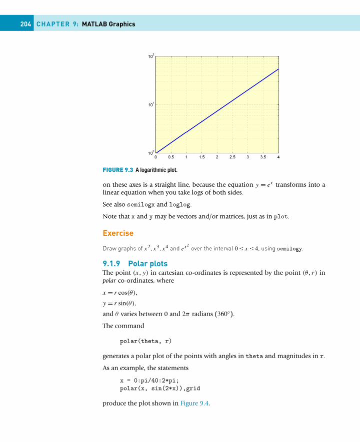
204 CHAPTER 9: MATLAB Graphics
FIGURE 9.3 A logarithmic plot.
on these axes is a straight line, because the equation y = ex transforms into alinear equation when you take logs of both sides.
See also semilogx and loglog.
Note that x and y may be vectors and/or matrices, just as in plot.
Exercise
Draw graphs of x2, x3, x4 and ex2over the interval 0 ≤ x ≤ 4, using semilogy.
9.1.9 Polar plotsThe point (x, y) in cartesian co-ordinates is represented by the point (θ, r) inpolar co-ordinates, where
x = r cos(θ),
y = r sin(θ),
and θ varies between 0 and 2π radians (360◦).
The command
polar(theta, r)
generates a polar plot of the points with angles in theta and magnitudes in r.
As an example, the statements
x = 0:pi/40:2*pi;polar(x, sin(2*x)),grid
produce the plot shown in Figure 9.4.
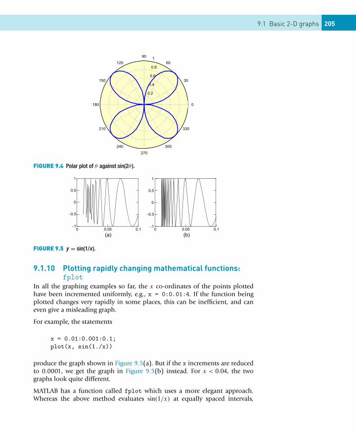
9.1 Basic 2-D graphs 205
FIGURE 9.4 Polar plot of θ against sin(2θ ).
FIGURE 9.5 y = sin(1/x ).
9.1.10 Plotting rapidly changing mathematical functions:fplot
In all the graphing examples so far, the x co-ordinates of the points plottedhave been incremented uniformly, e.g., x = 0:0.01:4. If the function beingplotted changes very rapidly in some places, this can be inefficient, and caneven give a misleading graph.
For example, the statements
x = 0.01:0.001:0.1;plot(x, sin(1./x))
produce the graph shown in Figure 9.5(a). But if the x increments are reducedto 0.0001, we get the graph in Figure 9.5(b) instead. For x < 0.04, the twographs look quite different.
MATLAB has a function called fplot which uses a more elegant approach.Whereas the above method evaluates sin(1/x) at equally spaced intervals,
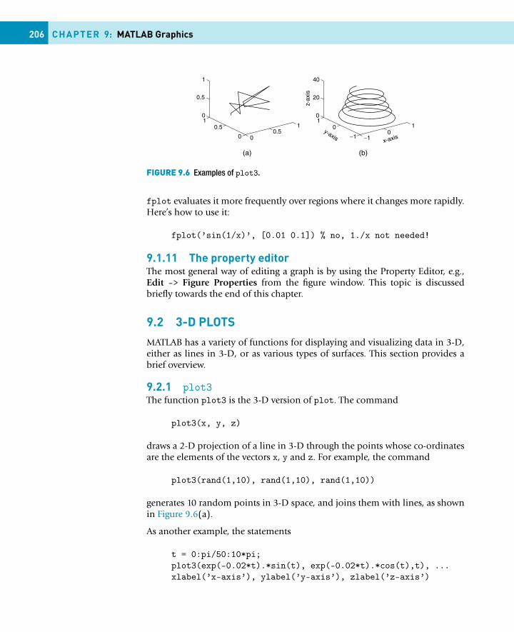
206 CHAPTER 9: MATLAB Graphics
FIGURE 9.6 Examples of plot3.
fplot evaluates it more frequently over regions where it changes more rapidly.Here’s how to use it:
fplot(’sin(1/x)’, [0.01 0.1]) % no, 1./x not needed!
9.1.11 The property editorThe most general way of editing a graph is by using the Property Editor, e.g.,Edit -> Figure Properties from the figure window. This topic is discussedbriefly towards the end of this chapter.
9.2 3-D PLOTS
MATLAB has a variety of functions for displaying and visualizing data in 3-D,either as lines in 3-D, or as various types of surfaces. This section provides abrief overview.
9.2.1 plot3The function plot3 is the 3-D version of plot. The command
plot3(x, y, z)
draws a 2-D projection of a line in 3-D through the points whose co-ordinatesare the elements of the vectors x, y and z. For example, the command
plot3(rand(1,10), rand(1,10), rand(1,10))
generates 10 random points in 3-D space, and joins them with lines, as shownin Figure 9.6(a).
As another example, the statements
t = 0:pi/50:10*pi;plot3(exp(-0.02*t).*sin(t), exp(-0.02*t).*cos(t),t), ...xlabel(’x-axis’), ylabel(’y-axis’), zlabel(’z-axis’)
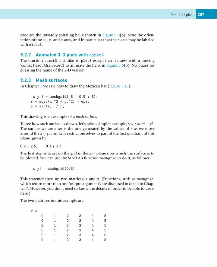
9.2 3-D plots 207
produce the inwardly spiraling helix shown in Figure 9.6(b). Note the orien-tation of the x-, y- and z-axes, and in particular that the z-axis may be labeledwith zlabel.
9.2.2 Animated 3-D plots with comet3The function comet3 is similar to plot3 except that it draws with a moving‘comet head’. Use comet3 to animate the helix in Figure 9.6(b). No prizes forguessing the name of the 2-D version.
9.2.3 Mesh surfacesIn Chapter 1 we saw how to draw the Mexican hat (Figure 1.13):
[x y ] = meshgrid(-8 : 0.5 : 8);r = sqrt(x.^2 + y.^2) + eps;z = sin(r) ./ r;
This drawing is an example of a mesh surface.
To see how such surface is drawn, let’s take a simpler example, say z = x2 − y2.The surface we are after is the one generated by the values of z as we movearound the x-y plane. Let’s restrict ourselves to part of the first quadrant of thisplane, given by
0 ≤ x ≤ 5, 0 ≤ y ≤ 5.
The first step is to set up the grid in the x-y plane over which the surface is tobe plotted. You can use the MATLAB function meshgrid to do it, as follows:
[x y] = meshgrid(0:5);
This statement sets up two matrices, x and y. (Functions, such as meshgrid,which return more than one ‘output argument’, are discussed in detail in Chap-ter 7. However, you don’t need to know the details in order to be able to use ithere.)
The two matrices in this example are:
x =0 1 2 3 4 50 1 2 3 4 50 1 2 3 4 50 1 2 3 4 50 1 2 3 4 50 1 2 3 4 5
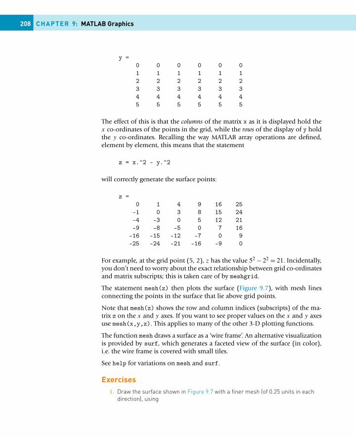
208 CHAPTER 9: MATLAB Graphics
y =0 0 0 0 0 01 1 1 1 1 12 2 2 2 2 23 3 3 3 3 34 4 4 4 4 45 5 5 5 5 5
The effect of this is that the columns of the matrix x as it is displayed hold thex co-ordinates of the points in the grid, while the rows of the display of y holdthe y co-ordinates. Recalling the way MATLAB array operations are defined,element by element, this means that the statement
z = x.^2 - y.^2
will correctly generate the surface points:
z =0 1 4 9 16 25
-1 0 3 8 15 24-4 -3 0 5 12 21-9 -8 -5 0 7 16-16 -15 -12 -7 0 9-25 -24 -21 -16 -9 0
For example, at the grid point (5, 2), z has the value 52 − 22 = 21. Incidentally,you don’t need to worry about the exact relationship between grid co-ordinatesand matrix subscripts; this is taken care of by meshgrid.
The statement mesh(z) then plots the surface (Figure 9.7), with mesh linesconnecting the points in the surface that lie above grid points.
Note that mesh(z) shows the row and column indices (subscripts) of the ma-trix z on the x and y axes. If you want to see proper values on the x and y axesuse mesh(x,y,z). This applies to many of the other 3-D plotting functions.
The function mesh draws a surface as a ‘wire frame’. An alternative visualizationis provided by surf, which generates a faceted view of the surface (in color),i.e. the wire frame is covered with small tiles.
See help for variations on mesh and surf.
Exercises1. Draw the surface shown in Figure 9.7 with a finer mesh (of 0.25 units in each
direction), using
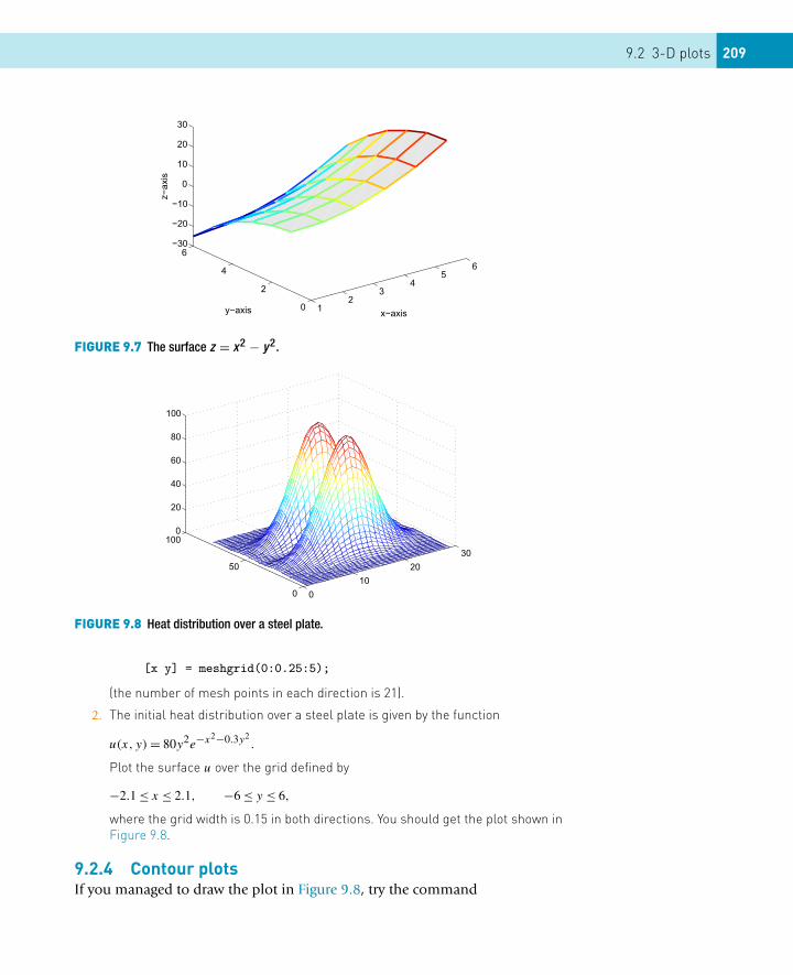
9.2 3-D plots 209
FIGURE 9.7 The surface z = x2 − y2.
FIGURE 9.8 Heat distribution over a steel plate.
[x y] = meshgrid(0:0.25:5);
(the number of mesh points in each direction is 21).
2. The initial heat distribution over a steel plate is given by the function
u(x, y) = 80y2e−x2−0.3y2.
Plot the surface u over the grid defined by
−2.1 ≤ x ≤ 2.1, −6 ≤ y ≤ 6,
where the grid width is 0.15 in both directions. You should get the plot shown inFigure 9.8.
9.2.4 Contour plotsIf you managed to draw the plot in Figure 9.8, try the command
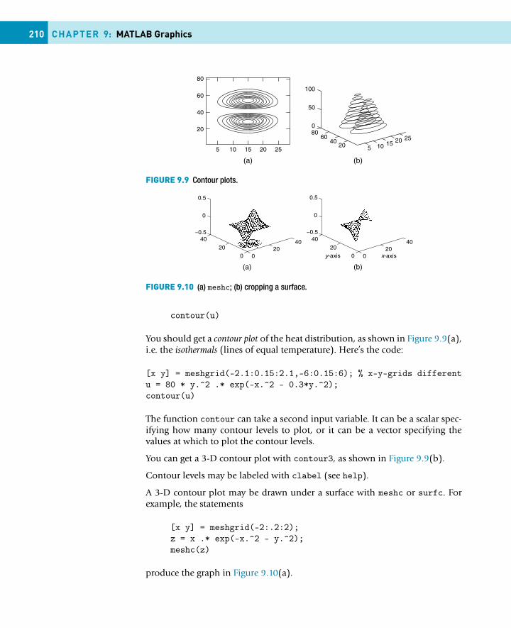
210 CHAPTER 9: MATLAB Graphics
FIGURE 9.9 Contour plots.
FIGURE 9.10 (a) meshc; (b) cropping a surface.
contour(u)
You should get a contour plot of the heat distribution, as shown in Figure 9.9(a),i.e. the isothermals (lines of equal temperature). Here’s the code:
[x y] = meshgrid(-2.1:0.15:2.1,-6:0.15:6); % x-y-grids differentu = 80 * y.^2 .* exp(-x.^2 - 0.3*y.^2);contour(u)
The function contour can take a second input variable. It can be a scalar spec-ifying how many contour levels to plot, or it can be a vector specifying thevalues at which to plot the contour levels.
You can get a 3-D contour plot with contour3, as shown in Figure 9.9(b).
Contour levels may be labeled with clabel (see help).
A 3-D contour plot may be drawn under a surface with meshc or surfc. Forexample, the statements
[x y] = meshgrid(-2:.2:2);z = x .* exp(-x.^2 - y.^2);meshc(z)
produce the graph in Figure 9.10(a).
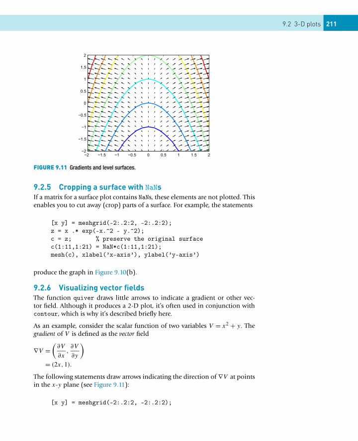
9.2 3-D plots 211
FIGURE 9.11 Gradients and level surfaces.
9.2.5 Cropping a surface with NaNsIf a matrix for a surface plot contains NaNs, these elements are not plotted. Thisenables you to cut away (crop) parts of a surface. For example, the statements
[x y] = meshgrid(-2:.2:2, -2:.2:2);z = x .* exp(-x.^2 - y.^2);c = z; % preserve the original surfacec(1:11,1:21) = NaN*c(1:11,1:21);mesh(c), xlabel(’x-axis’), ylabel(’y-axis’)
produce the graph in Figure 9.10(b).
9.2.6 Visualizing vector fieldsThe function quiver draws little arrows to indicate a gradient or other vec-tor field. Although it produces a 2-D plot, it’s often used in conjunction withcontour, which is why it’s described briefly here.
As an example, consider the scalar function of two variables V = x2 + y. Thegradient of V is defined as the vector field
∇V =(
∂V
∂x,∂V
∂y
)
= (2x,1).
The following statements draw arrows indicating the direction of ∇V at pointsin the x-y plane (see Figure 9.11):
[x y] = meshgrid(-2:.2:2, -2:.2:2);
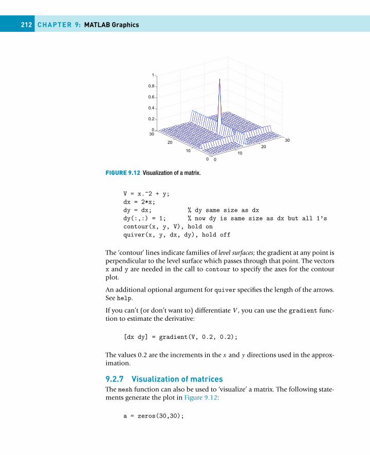
212 CHAPTER 9: MATLAB Graphics
FIGURE 9.12 Visualization of a matrix.
V = x.^2 + y;dx = 2*x;dy = dx; % dy same size as dxdy(:,:) = 1; % now dy is same size as dx but all 1’scontour(x, y, V), hold onquiver(x, y, dx, dy), hold off
The ‘contour’ lines indicate families of level surfaces; the gradient at any point isperpendicular to the level surface which passes through that point. The vectorsx and y are needed in the call to contour to specify the axes for the contourplot.
An additional optional argument for quiver specifies the length of the arrows.See help.
If you can’t (or don’t want to) differentiate V , you can use the gradient func-tion to estimate the derivative:
[dx dy] = gradient(V, 0.2, 0.2);
The values 0.2 are the increments in the x and y directions used in the approx-imation.
9.2.7 Visualization of matricesThe mesh function can also be used to ‘visualize’ a matrix. The following state-ments generate the plot in Figure 9.12:
a = zeros(30,30);
9.2 3-D plots 213
a(:,15) = 0.2*ones(30,1);a(7,:) = 0.1*ones(1,30);a(15,15) = 1;mesh(a)
The matrix a is 30 × 30. The element in the middle—a(15,15)—is 1, all theelements in row 7 are 0.1, and all the remaining elements in column 15 are0.2. mesh(a) then interprets the rows and columns of a as an x-y co-ordinategrid, with the values a(i,j) forming the mesh surface above the points (i, j).
The function spy is useful for visualizing sparse matrices.
9.2.8 Rotation of 3-D graphsThe view function enables you to specify the angle from which you view a 3-D graph. To see it in operation, run the following program, which rotates thevisualized matrix in Figure 9.12:
a = zeros(30,30);a(:,15) = 0.2*ones(30,1);a(7,:) = 0.1*ones(1,30);a(15,15) = 1;el = 30;for az = -37.5:15:-37.5+360
mesh(a), view(az, el)pause(0.5)
end
The function view takes two arguments. The first one, az in this example, iscalled the azimuth or polar angle in the x-y plane (in degrees). az rotates theviewpoint (you) about the z-axis—i.e. about the ‘pinnacle’ at (15,15) in Fig-ure 9.12—in a counter-clockwise direction. The default value of az is −37.5◦.The program therefore rotates you in a counter-clockwise direction about thez-axis in 15◦ steps starting at the default position.
The second argument of view is the vertical elevation el (in degrees). This isthe angle a line from the viewpoint makes with the x-y plane. A value of 90◦for el means you are directly overhead. Positive values of the elevation meanyou are above the x-y plane; negative values mean you are below it. The defaultvalue of el is 30◦.
The command pause(n) suspends execution for n seconds.
You can rotate a 3-D figure interactively as follows. Click the Rotate 3-D buttonin the figure toolbar (first button from the right). Click on the axes and anoutline of the figure appears to help you visualize the rotation. Drag the mouse
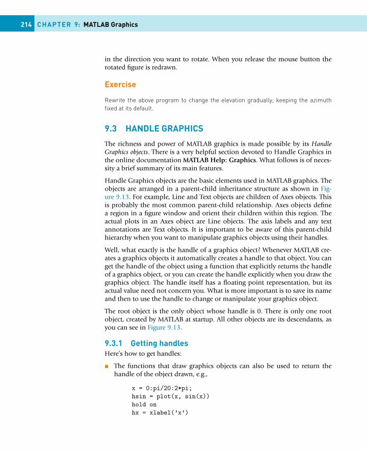
214 CHAPTER 9: MATLAB Graphics
in the direction you want to rotate. When you release the mouse button therotated figure is redrawn.
Exercise
Rewrite the above program to change the elevation gradually, keeping the azimuthfixed at its default.
9.3 HANDLE GRAPHICS
The richness and power of MATLAB graphics is made possible by its HandleGraphics objects. There is a very helpful section devoted to Handle Graphics inthe online documentation MATLAB Help: Graphics. What follows is of neces-sity a brief summary of its main features.
Handle Graphics objects are the basic elements used in MATLAB graphics. Theobjects are arranged in a parent-child inheritance structure as shown in Fig-ure 9.13. For example, Line and Text objects are children of Axes objects. Thisis probably the most common parent-child relationship. Axes objects definea region in a figure window and orient their children within this region. Theactual plots in an Axes object are Line objects. The axis labels and any textannotations are Text objects. It is important to be aware of this parent-childhierarchy when you want to manipulate graphics objects using their handles.
Well, what exactly is the handle of a graphics object? Whenever MATLAB cre-ates a graphics objects it automatically creates a handle to that object. You canget the handle of the object using a function that explicitly returns the handleof a graphics object, or you can create the handle explicitly when you draw thegraphics object. The handle itself has a floating point representation, but itsactual value need not concern you. What is more important is to save its nameand then to use the handle to change or manipulate your graphics object.
The root object is the only object whose handle is 0. There is only one rootobject, created by MATLAB at startup. All other objects are its descendants, asyou can see in Figure 9.13.
9.3.1 Getting handlesHere’s how to get handles:
� The functions that draw graphics objects can also be used to return thehandle of the object drawn, e.g.,
x = 0:pi/20:2*pi;hsin = plot(x, sin(x))hold onhx = xlabel(’x’)
9.3 Handle graphics 215
FIGURE 9.13 Parent-child relationships of Handle Graphics objects (from top to bottom).
hsin is the handle of the Line object (the sine graph), and hx is the handleof the Text object (the x axis label) in the current Axes object.The command
figure(h)
where h is an integer, creates a new figure, or makes figure h the currentfigure. h is the handle of the figure object.
� There are three functions that return the handle of particular graphics ob-jects:gcf gets the handle of the current figure, e.g.,
hf = gcf;
gca gets the handle of the current axes.gco gets the handle of the current graphics object, which is the last graph-
ics object created or clicked on. For example, draw the sine graphabove and get its handle hsin. Click on the graph in the figure win-dow. Then enter the command
ho = gco
in the Command Window. ho should be set to the handle of the sinegraph (it should have the same numeric value as hsin).
9.3.2 Graphics object properties and how to change themOnce you have the handle of a graphics object you can use it to change theproperties of that object. As an example, draw a sine graph and get its handle,as demonstrated above:
x = 0:pi/20:2*pi;hsin = plot(x, sin(x))
Now suppose you want to make the graph much thicker. Enter the followingcommand:
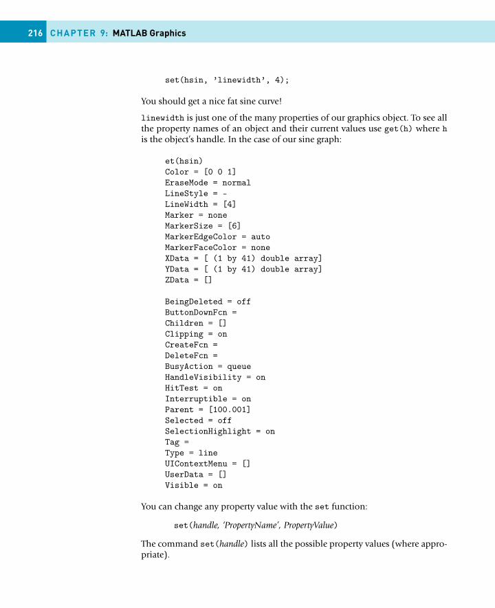
216 CHAPTER 9: MATLAB Graphics
set(hsin, ’linewidth’, 4);
You should get a nice fat sine curve!
linewidth is just one of the many properties of our graphics object. To see allthe property names of an object and their current values use get(h) where his the object’s handle. In the case of our sine graph:
et(hsin)Color = [0 0 1]EraseMode = normalLineStyle = -LineWidth = [4]Marker = noneMarkerSize = [6]MarkerEdgeColor = autoMarkerFaceColor = noneXData = [ (1 by 41) double array]YData = [ (1 by 41) double array]ZData = []
BeingDeleted = offButtonDownFcn =Children = []Clipping = onCreateFcn =DeleteFcn =BusyAction = queueHandleVisibility = onHitTest = onInterruptible = onParent = [100.001]Selected = offSelectionHighlight = onTag =Type = lineUIContextMenu = []UserData = []Visible = on
You can change any property value with the set function:
set(handle, ‘PropertyName’, PropertyValue)
The command set(handle) lists all the possible property values (where appro-priate).
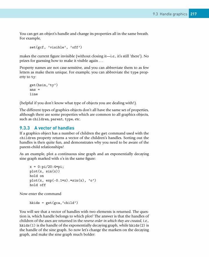
9.3 Handle graphics 217
You can get an object’s handle and change its properties all in the same breath.For example,
set(gcf, ’visible’, ’off’)
makes the current figure invisible (without closing it—i.e., it’s still ‘there’). Noprizes for guessing how to make it visible again . . .
Property names are not case-sensitive, and you can abbreviate them to as fewletters as make them unique. For example, you can abbreviate the type prop-erty to ty:
get(hsin,’ty’)ans =line
(helpful if you don’t know what type of objects you are dealing with!).
The different types of graphics objects don’t all have the same set of properties,although there are some properties which are common to all graphics objects,such as children, parent, type, etc.
9.3.3 A vector of handlesIf a graphics object has a number of children the get command used with thechildren property returns a vector of the children’s handles. Sorting out thehandles is then quite fun, and demonstrates why you need to be aware of theparent-child relationships!
As an example, plot a continuous sine graph and an exponentially decayingsine graph marked with o’s in the same figure:
x = 0:pi/20:4*pi;plot(x, sin(x))hold onplot(x, exp(-0.1*x).*sin(x), ’o’)hold off
Now enter the command
hkids = get(gca,’child’)
You will see that a vector of handles with two elements is returned. The ques-tion is, which handle belongs to which plot? The answer is that the handles ofchildren of the axes are returned in the reverse order in which they are created, i.e.,hkids(1) is the handle of the exponentially decaying graph, while hkids(2) isthe handle of the sine graph. So now let’s change the markers on the decayinggraph, and make the sine graph much bolder:
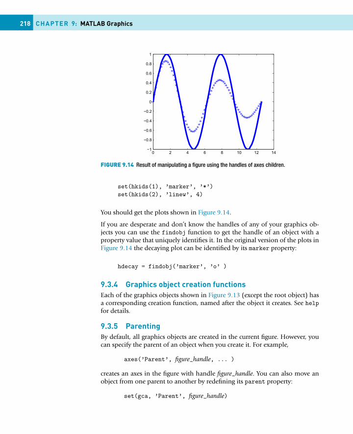
218 CHAPTER 9: MATLAB Graphics
FIGURE 9.14 Result of manipulating a figure using the handles of axes children.
set(hkids(1), ’marker’, ’*’)set(hkids(2), ’linew’, 4)
You should get the plots shown in Figure 9.14.
If you are desperate and don’t know the handles of any of your graphics ob-jects you can use the findobj function to get the handle of an object with aproperty value that uniquely identifies it. In the original version of the plots inFigure 9.14 the decaying plot can be identified by its marker property:
hdecay = findobj(’marker’, ’o’ )
9.3.4 Graphics object creation functionsEach of the graphics objects shown in Figure 9.13 (except the root object) hasa corresponding creation function, named after the object it creates. See helpfor details.
9.3.5 ParentingBy default, all graphics objects are created in the current figure. However, youcan specify the parent of an object when you create it. For example,
axes(’Parent’, figure_handle, ... )
creates an axes in the figure with handle figure_handle. You can also move anobject from one parent to another by redefining its parent property:
set(gca, ’Parent’, figure_handle)
9.3 Handle graphics 219
9.3.6 Positioning figuresAt startup MATLAB determines the default position and size of the figure win-dow, according to the size of your computer screen. You can change this bysetting the Position property of the figure object.
Before you tamper with the figure’s Position property you need to know thedimensions of your screen—this is one of the root object’s properties. For ex-ample,
get(0, ’screensize’)ans =
1 1 800 600
i.e., my screen is 800 by 600 pixels. The units of Screensize are pixels by de-faults. You can (naturally) change the units by setting the root’s Units property.For example,
set(0, ’units’, ’normalized’)
normalizes the width and height of the screen to 1. This is useful when you arewriting an M-file which is to be run on different computer systems.
Having sorted out the size of your screen, you can then fiddle with the figurePosition property, which is defined as a vector
[left bottom width height]
left and bottom define the position of the first addressable pixel in the lowerleft corner of the window, specified with respect to the lower left corner ofthe screen. width and height define the size of the interior of the window(excluding the window border).
You can normalize the figure’s Unit property as well as the root’s Unit property.You can then position figures absolutely, without reference to variations inscreen size. For example, the following code normalizes units and creates twofigures in the upper half of the screen:
set(0, ’units’, ’normalized’)h1 = figure(’units’, ’normalized’, ’visible’, ’off’)h2 = figure(’units’, ’normalized’, ’visible’, ’off’)set(h1, ’position’, [0.05 0.5 0.45 0.35], ’visible’, ’on’)set(h2, ’position’, [0.53 0.5 0.45 0.35], ’visible’, ’on’)
Note that the Visible property is first set to off to avoid the figures beingdrawn in the default position when they are created. They are only drawn when
220 CHAPTER 9: MATLAB Graphics
their positions have been redefined. Alternatively you can do everything whenthe figures are created:
h1 = figure(’un’, ’normalized’, ’pos’, [0.05 0.5 0.45 0.35])
9.4 EDITING PLOTS
There are a number of ways of editing plots.
9.4.1 Plot edit modeTo see how this works draw a graph, e.g., the friendly old sine. There are severalways to activate plot edit mode:
� Select Tools -> Edit Plot in the figure window.� Click on the Edit Plot selection button in the figure window toolbar (arrow
pointing roughly north-west).� Run the plotedit command in the Command Window.
When a figure is in plot edit mode the toolbar selection button is highlighted.Once you are in plot edit mode select an object by clicking on it. Selectionhandles will appear on the selected object.
As an exercise, get the sine graph into plot edit mode and try the following:
� Select the graph (click on it). Selection handles should appear.� Right click on the selected object (the graph). A context menu appears.� Use the context menu to change the graph’s line style and color.� Use the Insert menu to insert a legend (although this makes more sense
where you have multiple plots in the figure).� Insert a text box inside the figure close to the graph as follows. Click on
the Insert Text selection button in the toolbar (the capital A). The cursorchanges shape to indicate that it is in text insertion mode. Move the in-sertion point until it touches the graph somewhere and click. A text boxappears. Enter some text in it.You can use a subset of TEX characters and commands in text objects. Forexample, the text xk in Figure 14.1 was produced with the string {\it x_k}.See the entry Text property under String[1] in the online Help for a listof an available TEX characters and commands.
� Having labeled the graph you can change the format of the labels. Selectthe label and right-click. Change the font size and font style.
� Play around with the Insert Arrow and Insert Line selection buttons on thetoolbar to see if you can insert lines and arrows on the graph.
To exit plot edit mode, click the selection button or uncheck the Edit Plotoption on the Tools menu.
9.4 Editing plots 221
9.4.2 Property EditorThe Property Editor is more general than plot edit mode. It enables you tochange object properties interactively, rather than with the set function. It isideal for preparing presentation graphics.
There are numerous ways of starting the Property Editor (you may already havestumbled onto some):
� If plot edit mode is enabled you can:– Double-click on an object.– Right-click on an object and select Properties from the context menu.
� Select Figure Properties, Axes Properties or Current Object Propertiesfrom the figure Edit menu.
� Run the propedit command on the command line.
To experiment with the Property Editor it will be useful to have multiple plotsin a figure:
x = 0:pi/20:2*pi;hsin = plot(x,sin(x))hold onhcos = plot(x,cos(x))hold off
Start the Property Editor and work through the following exercises:
� The navigation bar at the top of the Property Editor (labeled Edit Propertiesfor:) identifies the object being edited. Click on the down arrow at the rightof the navigation bar to see all the objects in the figure. You will notice thatthere are two line objects. Immediately we are faced with the problem ofidentifying the two line objects in our figure. The answer is to give each ofthem tags by setting their Tag properties.Go back to the figure and select the sine graph. Back in the Property Editorthe navigation bar indicates you are editing one of the line objects. You willsee three tabs below the navigation bar: Data, Style and Info. Click the Infotab, and enter a label in the Tag box, e.g., sine. Press Enter. The tag sineimmediately appears next to the selected line object in the navigation bar.Give the cosine graph a tag as well (start by selecting the other line object).
� Select the sine graph. This time select the Style tab and go beserk changingits color, line style, line width and markers.
� Now select the axes object. Use the Labels tab to insert some axis labels.Use the Scale tab to change the y axis limits, for example.Note that if you were editing a 3-D plot you would be able to use the View-point tab to change the viewing angle and to set various camera properties.
Have fun!
222 CHAPTER 9: MATLAB Graphics
9.5 ANIMATION
There are three facilities for animation in MATLAB:
� The comet and comet3 functions can be used to draw comet plots.� The getframe function may be used to generate ‘movie frames’ from a se-
quence of graphs. The movie function can then be used to play back themovie a specified number of times.The MATLAB online documentation has the following script in MATLABHelp: Graphics: Creating Specialized Plots: Animation. It generates 16frames from the Fast Fourier Transforms of complex matrices:
for k = 1:16plot(fft(eye(k+16)))axis equalM(k) = getframe;
end
Now play it back, say five times:
movie(M, 5)
You can specify the speed of the playback, among other things. See help.� The most versatile (and satisfying) way of creating animations is by using
the Handle Graphics facilities. Two examples follow.
9.5.1 Animation with Handle GraphicsFor starters, run the following script, which should show the marker o tracingout a sine curve, leaving a trail behind it:
% animated sine graphx = 0;y = 0;dx = pi/40;p = plot(x, y, ’o’, ’EraseMode’, ’none’);
% ’xor’ shows only current point% ’ none’ shows all points
axis([0 20*pi -2 2])
for x = dx:dx:20*pi;x = x + dx;y = sin(x);set(p, ’XData’, x, ’YData’, y)drawnow
end
Note:
9.5 Animation 223
� The statement
p = plot(x, y, ’o’, ’EraseMode’, ’none’);
achieves a number of things. It plots the first point of the graph. It savesthe handle p of the plot for further reference. And it specifies that theErasemode property is none, i.e., the object must not be erased when itis drawn again. To achieve complete animation, set this property to xor—try it now. Then the object is erased each time it is redrawn (in a slightlydifferent position), creating the classic animation effect.
� The statement
set(p, ’XData’, x, ’YData’, y)
sets the x and y data values of the object p to the new values generated in thefor loop, and ‘redraws’ the object. However, it is not drawn on the screenimmediately—it joins the ‘event queue’, where it waits until it is flushedout.
� Finally, the drawnow function flushes the event queue and draws the objecton the screen so that we can see the fruit of our labors.As help drawnow will reveal, there are four events that flush the eventqueue:� a return to the MATLAB prompt—this is how you have seen all the
graphs you’ve drawn up to now;� hitting a pause statement;� executing a getframe command;� executing a drawnow command.For example, you could make the marker move in a more stately fashion byreplacing drawnow with pause(0.05)—that’s 0.05 s.
The next example is based on one in the Animation section of the MATLABdocumentation. It involves chaotic motion described by a system of three non-linear differential equations having a ‘strange attractor’ (known as the Lorenzstrange attractor). The system can be written as
dy
dt= Ay,
where y(t) is a vector with three components, and A is a matrix dependingon y:
A(y) =⎡⎣ −8/3 0 y(2)
0 −10 10−y(2) 28 −1
⎤⎦ .
The following script solves the system approximately using Euler’s method(a more accurate numerical solution is discussed in Chapter 14), and shows thesolution orbiting about two different attractors without settling into a steady
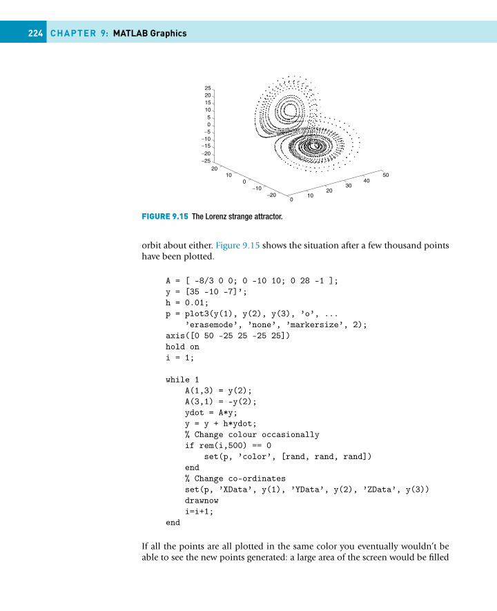
224 CHAPTER 9: MATLAB Graphics
FIGURE 9.15 The Lorenz strange attractor.
orbit about either. Figure 9.15 shows the situation after a few thousand pointshave been plotted.
A = [ -8/3 0 0; 0 -10 10; 0 28 -1 ];y = [35 -10 -7]’;h = 0.01;p = plot3(y(1), y(2), y(3), ’o’, ...
’erasemode’, ’none’, ’markersize’, 2);axis([0 50 -25 25 -25 25])hold oni = 1;
while 1A(1,3) = y(2);A(3,1) = -y(2);ydot = A*y;y = y + h*ydot;% Change colour occasionallyif rem(i,500) == 0
set(p, ’color’, [rand, rand, rand])end% Change co-ordinatesset(p, ’XData’, y(1), ’YData’, y(2), ’ZData’, y(3))drawnowi=i+1;
end
If all the points are all plotted in the same color you eventually wouldn’t beable to see the new points generated: a large area of the screen would be filled
9.6 Color etc. 225
with the drawing color. The color is therefore set randomly after every 500points are plotted.
9.6 COLOR ETC.
9.6.1 ColormapsMATLAB graphics can generate a rich variety of colors. You may be wonderinghow.
The following script shows a view of the Earth from space:
load earthimage(X); colormap(map)axis image
(axis image is the same as axis equal except that the plot box fits tightlyaround the data). For a variation use hot as the argument of colormap insteadof map.
The matrix X loaded from earth is 257-by-250. Each of the elements of X isan integer in the range 1–64. For example, here is a 3-by-3 submatrix of X(somewhere in north-east Africa):
X(39:41,100:102)ans =
14 15 1410 16 1010 10 10
The colormap function generates by default a 64-by-3 matrix with elementsin the range 0–1. The values in the three columns represent the intensities ofthe red, green and blue (RGB) video components respectively. Each row of thismatrix therefore defines a particular color by specifying its RGB components.The image function maps each element of its argument to a row in the col-ormap to find the color of that element. For example, X(40,101) has the value16. Row 16 of the colormap has the three values
0.6784 0.3216 0.1922
(reddish) as you can easily verify with the statements
cm = colormap(map);cm(16,:)
226 CHAPTER 9: MATLAB Graphics
(The map colormap is also loaded from earth.) These values of RGB specifythe color of the pixel 40 from the top and 101 from the left in the figure.Incidentally, you can use the statement
[xp yp] = ginput
to get the co-ordinates of a point in the figure (crosshairs appears in the figure;click on the point whose co-ordinates you want). Clicking on the point innorth-east Africa results in
xp =101.8289 % from the left (column of X)
yp =40.7032 % from the top (row of X)
Note that xp and yp correspond to the columns and rows of X respectively (imag-ine the matrix X superimposed on the figure).
There are a number of functions provided by MATLAB which generate col-ormaps, e.g., jet (the default), bone, flag, prism. See help graph3d for acomplete list.
You can sample the various colormaps quite nicely with the following state-ment, which shows 64 vertical strips, each in a different color:
image(1:64),colormap(prism)
Or why not generate some random colors?
randmap(:,1) = rand(64,1);randmap(:,2) = rand(64,1);randmap(:,3) = rand(64,1);image(1:64);colormap(randmap)
The function colorbar displays the current colormap vertically or horizontallyin the figure with your graph, indicating how the 64 colors are mapped. Try itwith the image of the Earth.
Note that 64 is the default length of a colormap. The functions that generatecolormaps have an optional parameter specifying the length of the colormap.
9.6.2 Color of surface plotsWhen you draw a surface plot with a single matrix argument, e.g., surf(z),the argument z specifies both the height of the surface and the color. As anexample use the function peaks which generates a surface with a couple ofpeaks and valleys:
9.6 Color etc. 227
z = peaks;surf(z), colormap(jet), colorbar
The colorbar indicates that the minimum element of z (somewhat less than−6) is mapped to row 1 of the colormap (R = 0, G = 0, B = 0.5625), whereasthe maximum element (about 8) is mapped to row 64 (R = 0.5625, G = 0,B = 0).
You can specify the color with a second argument the same size as the first:
z = peaks(16); % generates a 16-by-16 meshc = rand(16);surf(z, c), colormap(prism)
Here the surface is tiled with a random pattern of 16-by-16 colors from theprism colormap.
In this form of surf each element of c is used to determine the color of thepoint in the corresponding element of z. By default MATLAB uses a processcalled scaled mapping to map from an element of z (or c) to the color in thecolormap. The details of the scaling are determined by the caxis command.For further details see help caxis or the section Coloring Mesh and SurfacePlots in MATLAB Help: 3-D Visualization: Creating 3-D Graphs.
You can exploit the facility to specify color in order to emphasize properties ofthe surface. The following example is given in the MATLAB documentation:
z = peaks(40);c = del2(z);surf(z, c)colormap hot
The function del2 computes the discrete Laplacian of a surface—the Laplacianis related to the curvature of the surface. Creating a color array from the Lapla-cian means that regions with similar curvature will be drawn in the same color.Compare the surface obtained this way with that produced by the statement
surf(P), colormap(hot)
In the second case regions with similar heights about the x-y plane have thesame color.
Alternative forms of surf (and related surface functions) are:
surf(x, y, z) % colour determined by zsurf(x, y, z, c) % colour determined by c
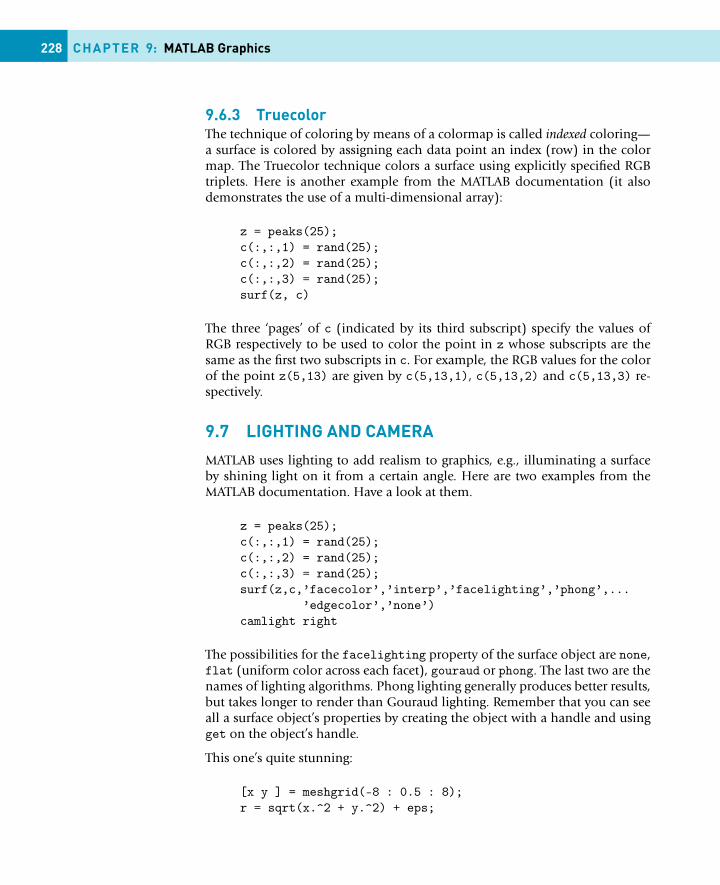
228 CHAPTER 9: MATLAB Graphics
9.6.3 TruecolorThe technique of coloring by means of a colormap is called indexed coloring—a surface is colored by assigning each data point an index (row) in the colormap. The Truecolor technique colors a surface using explicitly specified RGBtriplets. Here is another example from the MATLAB documentation (it alsodemonstrates the use of a multi-dimensional array):
z = peaks(25);c(:,:,1) = rand(25);c(:,:,2) = rand(25);c(:,:,3) = rand(25);surf(z, c)
The three ‘pages’ of c (indicated by its third subscript) specify the values ofRGB respectively to be used to color the point in z whose subscripts are thesame as the first two subscripts in c. For example, the RGB values for the colorof the point z(5,13) are given by c(5,13,1), c(5,13,2) and c(5,13,3) re-spectively.
9.7 LIGHTING AND CAMERA
MATLAB uses lighting to add realism to graphics, e.g., illuminating a surfaceby shining light on it from a certain angle. Here are two examples from theMATLAB documentation. Have a look at them.
z = peaks(25);c(:,:,1) = rand(25);c(:,:,2) = rand(25);c(:,:,3) = rand(25);surf(z,c,’facecolor’,’interp’,’facelighting’,’phong’,...
’edgecolor’,’none’)camlight right
The possibilities for the facelighting property of the surface object are none,flat (uniform color across each facet), gouraud or phong. The last two are thenames of lighting algorithms. Phong lighting generally produces better results,but takes longer to render than Gouraud lighting. Remember that you can seeall a surface object’s properties by creating the object with a handle and usingget on the object’s handle.
This one’s quite stunning:
[x y ] = meshgrid(-8 : 0.5 : 8);r = sqrt(x.^2 + y.^2) + eps;
9.8 Saving, printing and exporting graphs 229
z = sin(r) ./ r;surf(x,y,z,’facecolor’,’interp’,’edgecolor’,’none’, ...
’facelighting’,’phong’)colormap jetdaspect([5 5 1])axis tightview(-50, 30)camlight left
For more information on lighting and the camera see the sections Lighting asa Visualization Tool and Defining the View in MATLAB Help: 3-D Visualiza-tion.
9.8 SAVING, PRINTING AND EXPORTING GRAPHS
9.8.1 Saving and opening figure filesYou can save a figure generated during a MATLAB session so that you can openit in a subsequent session. Such a file has the .fig extension.
� Select Save from the figure window File menu.� Make sure the Save as type is .fig.
To open a figure file select Open from the File menu.
9.8.2 Printing a graphYou can print everything inside a figure window frame, including axis labelsand annotations:
� To print a figure select Print from the figure window File menu.� If you have a black and white printer, colored lines and text are ‘dithered to
gray’ which may not print very clearly in some cases. In that case select PageSetup from the figure File menu. Select the Lines and Text tab and click onthe Black and white option for Convert solid colored lines to:.
9.8.3 Exporting a graphA figure may be exported in one of a number of graphics formats if you wantto import it into another application, such as a text processor. You can alsoexport it to the Windows clipboard and paste it from there into an application.
To export to the clipboard:
� Select Copy Figure from the figure window’s Edit menu (this action copiesto the clipboard).
� Before you copy to the clipboard you may need to adjust the figure’s set-tings. You can do this by selecting Preferences from the figure’s File menu.This action opens the Preferences panel, from which you can select Figure

230 CHAPTER 9: MATLAB Graphics
Copy Template Preferences and Copy Options Preferences to adjust thefigure’s settings.You may also have to adjust further settings with Page Setup from the fig-ure’s File menu.
To export a figure to a file in a specific graphics format:
� Select Export from the figure’s File menu. This action invokes the Exportdialog box.
� Select a graphics format from the Save as type list, e.g., EMF (enhancedmetafiles), JPEG, etc. You may need to experiment to find the best formatfor the target application you have in mind.For example, to insert a figure into a Word document, I find it much easierfirst to save it in EMF or JPEG format and then to insert the graphics fileinto the Word document, rather than to go the clipboard route (there aremore settings to adjust that way).
For further details consult the section Basic Printing and Exporting in MAT-LAB Help: Graphics.
SUMMARY� 2-D plots are drawn with the plot statement.� There is a set of easy-to-use plotters called ez*.� Graphs may be labeled with grid, text, title, xlabel, ylabel, etc.� Multiple plots may be drawn on the same axes in a number of ways.� Line styles, markers and color may be varied.� Axis limits may be set explicitly.� In MATLAB the word ‘axes’ refers to the graphics object in which the x and
y axis and their labels, plots and text annotations are drawn.� A number of axes may be drawn in the same figure with subplot.� Co-ordinates of points in a figure may be selected with ginput.� semilogx, semilogy and loglog are used to plot on log10 scales.� The polar command plots in polar co-ordinates.� fplot provides a handy way of plotting mathematical functions.� plot3 draws lines in 3-D.� comet3 animates a 3-D plot.� A 3-D surface may be plotted with mesh.� A 3-D plot may be rotated with view or with the Rotate 3-D tool in the
figure window.� mesh may also be used to visualize a matrix.� contour and contour3 draws contour levels in 2-D and 3-D respectively.� 3-D surfaces may be cropped.� For a complete list of graphics functions consult the online Help in MAT-
LAB Function Reference: Functions by Category: Graphics.� MATLAB graphics objects are arranged in a parent-child hierarchy.
9.8 Exercises 231
� A handle may be attached to a graphics object at creation; the handle maybe used to manipulate the graphics object.
� If h is the handle of a graphics object, get(h) returns all the current valuesof the object’s properties. set(h) shows you all the possible values of theproperties.
� The functions gcf, gca and gco return the handles of various graphics ob-jects.
� Use set to change the properties of a graphics object.� A graph may be edited to a limited extent in plot edit mode, selected from
the figure window (Tools -> Edit Plot). More general editing can be donewith the Property Editor (Edit -> Figure Properties from the figure win-dow).
� The most versatile way to create animations is by using the Handle Graphicsfacilities. Other techniques involve comet plots and movies.
� Indexed coloring may be done with colormaps.� Graphs saved to .fig files may be opened in subsequent MATLAB sessions.� Graphs may be exported to the Windows clipboard, or to files in a variety
of graphics formats.
EXERCISES9.1 Draw a graph of the population of the USA from 1790 to 2000, using the
(logistic) model
P(t) = 19 72 73 000
1 + e−0.03134(t−1913.25)
where t is the date in years.Actual data (in 1000s) for every decade from 1790 to 1950 are as follows:3929, 5308, 7240, 9638, 12 866, 17 069, 23 192, 31 443, 38 558, 50 156,62 948, 75 995, 91 972, 1 05 711, 1 22 775, 1 31 669, 1 50 697. Superim-pose this data on the graph of P(t). Plot the data as discrete circles (i.e.do not join them with lines) as shown in Figure 9.16.
9.2 The Spiral of Archimedes (Figure 9.17) may be represented in polar co-ordinates by the equation
r = aθ,
where a is some constant. (The shells of a class of animals called num-mulites grow in this way.) Write some command-line statements to drawthe spiral for some values of a.
9.3 Another type of spiral is the logarithmic spiral (Figure 9.17), which de-scribes the growth of shells of animals like the periwinkle and the nautilus.Its equation in polar co-ordinates is
r = aqθ ,
where a > 0, q > 1. Draw this spiral.
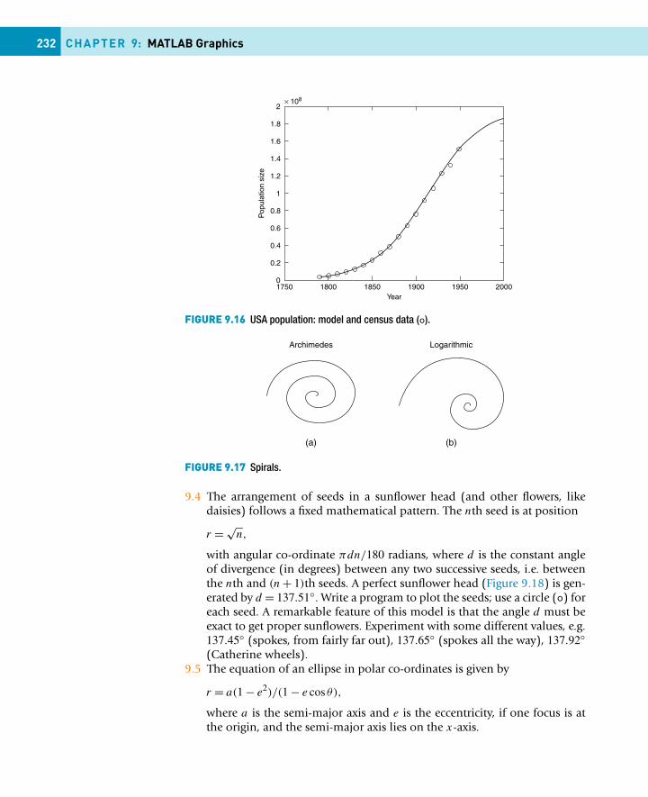
232 CHAPTER 9: MATLAB Graphics
FIGURE 9.16 USA population: model and census data (o).
FIGURE 9.17 Spirals.
9.4 The arrangement of seeds in a sunflower head (and other flowers, likedaisies) follows a fixed mathematical pattern. The nth seed is at position
r = √n,
with angular co-ordinate πdn/180 radians, where d is the constant angleof divergence (in degrees) between any two successive seeds, i.e. betweenthe nth and (n + 1)th seeds. A perfect sunflower head (Figure 9.18) is gen-erated by d = 137.51◦. Write a program to plot the seeds; use a circle (o) foreach seed. A remarkable feature of this model is that the angle d must beexact to get proper sunflowers. Experiment with some different values, e.g.137.45◦ (spokes, from fairly far out), 137.65◦ (spokes all the way), 137.92◦(Catherine wheels).
9.5 The equation of an ellipse in polar co-ordinates is given by
r = a(1 − e2)/(1 − e cos θ),
where a is the semi-major axis and e is the eccentricity, if one focus is atthe origin, and the semi-major axis lies on the x-axis.
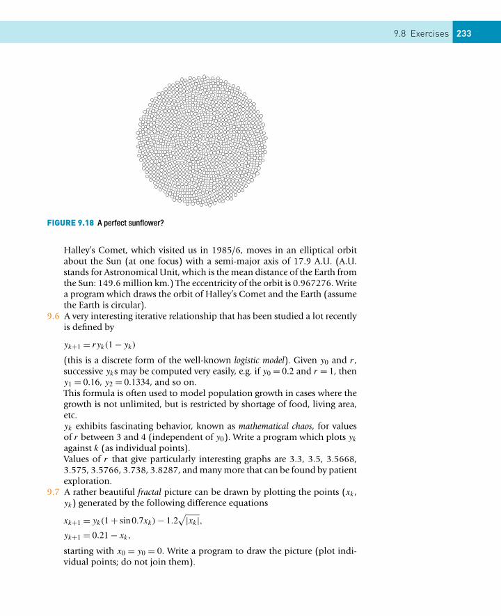
9.8 Exercises 233
FIGURE 9.18 A perfect sunflower?
Halley’s Comet, which visited us in 1985/6, moves in an elliptical orbitabout the Sun (at one focus) with a semi-major axis of 17.9 A.U. (A.U.stands for Astronomical Unit, which is the mean distance of the Earth fromthe Sun: 149.6 million km.) The eccentricity of the orbit is 0.967276. Writea program which draws the orbit of Halley’s Comet and the Earth (assumethe Earth is circular).
9.6 A very interesting iterative relationship that has been studied a lot recentlyis defined by
yk+1 = ryk(1 − yk)
(this is a discrete form of the well-known logistic model). Given y0 and r ,successive yks may be computed very easily, e.g. if y0 = 0.2 and r = 1, theny1 = 0.16, y2 = 0.1334, and so on.This formula is often used to model population growth in cases where thegrowth is not unlimited, but is restricted by shortage of food, living area,etc.yk exhibits fascinating behavior, known as mathematical chaos, for valuesof r between 3 and 4 (independent of y0). Write a program which plots yk
against k (as individual points).Values of r that give particularly interesting graphs are 3.3, 3.5, 3.5668,3.575, 3.5766, 3.738, 3.8287, and many more that can be found by patientexploration.
9.7 A rather beautiful fractal picture can be drawn by plotting the points (xk ,yk) generated by the following difference equations
xk+1 = yk(1 + sin 0.7xk) − 1.2√|xk|,
yk+1 = 0.21 − xk,
starting with x0 = y0 = 0. Write a program to draw the picture (plot indi-vidual points; do not join them).
CONTENTS
Updateprocesses ........... 235Unit time steps ...... 236Non-unit timesteps ...................... 238Using a function .... 239Exact solution........ 241
Frequencies, barcharts andhistograms ......... 242A random walk ...... 242Histograms............ 243
Sorting................. 244Bubble Sort ........... 244MATLAB’s sort ...... 246
Structures .......... 247
Cell arrays.......... 249Assigning data to cellarrays .................... 249Accessing data in cellarrays .................... 250Using cell arrays ... 251Displaying andvisualizing cellarrays .................... 252
Classes andobjects ................. 252
CHAPTER 10
Vectors as Arrays and Other Data Structures
THE OBJECTIVES OF THIS CHAPTER ARE:
� To enable you to solve problems which involve working carefully witharray subscripts.
� To introduce you to:– Structures.– Cells and cell arrays.
In MATLAB an array is just another name for a vector. So why have a large partof a chapter on arrays, when we have already been using vectors for most ofthe book? It is helpful to talk about arrays (as opposed to vectors) when weare concerned with handling individual elements by means of their subscripts,rather than with the vector as a whole. Thus, in the first three sections of thischapter we look at a number of problems which are best solved by treatingvectors as arrays, usually with the help of for loops.
In the last three sections of this chapter we deal with other, more advanced,data structures.
10.1 UPDATE PROCESSES
In Chapter 8 (Update processes) we considered the problem of calculating thetemperature of orange juice (OJ) in a can as it cools in a fridge. This is an ex-ample of an update process, where the main variable is repeatedly updated overa period of time. We now examine how to solve this problem more generally.
The OJ is initially at temperature 25 ◦C when it is placed in the fridge, wherethe ambient temperature F is 10◦. The standard way to solve such an updateprocess is to break the time period up into a number of small steps, each oflength dt. If Ti is the temperature at the beginning of step i, we can get Ti+1
from Ti as follows:235
Essential MATLAB for Engineers and Scientists. DOI:10.1016/B978-0-08-100877-5.00011-6Copyright © 2017 Daniel T. Valentine. Published by Elsevier Ltd. All rights reserved.
Summary ............ 253
236 CHAPTER 10: Vectors as Arrays and Other Data Structures
Ti+1 = Ti − K dt (Ti − F), (10.1)
where K is a physical constant, and units are chosen so that time is in minutes.
10.1.1 Unit time stepsWe first solve the problem using a unit time step, i.e., dt = 1. The simplestway is to use scalars for the time and the temperature, as we saw in Chapter 8(although we didn’t use a unit time step there):
K = 0.05;F = 10;T = 25; % initial temperature of OJ
for time = 1:100 % time in minutesT = T - K * (T - F); % dt = 1if rem(time, 5) == 0
disp( [time T] )end
end;
Note the use of rem to display the results every 5 minutes: when time is aninteger multiple of 5 its remainder when divided by 5 will be zero.
While this is undoubtedly the easiest way of writing the script, we cannot easilyplot the graph of temperature against time. In order to do that, time and Tmust be vectors. The index of the for loop must be used as the subscript ofeach element of T. Here’s the script (update1.m):
K = 0.05;F = 10;time = 0:100; % initialize vector timeT = zeros(1,101); % pre-allocate vector TT(1) = 25; % initial temperature of OJ
for i = 1:100 % time in minutesT(i+1) = T(i) - K * (T(i) - F); % construct T
end;
disp([ time(1:5:101)’ T(1:5:101)’ ]); % display resultsplot(time, T), grid % every 5 mins
See Figure 10.1 for typical graphs.
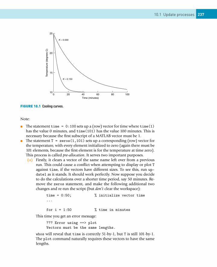
10.1 Update processes 237
FIGURE 10.1 Cooling curves.
Note:
� The statement time = 0:100 sets up a (row) vector for time where time(1)has the value 0 minutes, and time(101) has the value 100 minutes. This isnecessary because the first subscript of a MATLAB vector must be 1.
� The statement T = zeros(1,101) sets up a corresponding (row) vector forthe temperature, with every element initialized to zero (again there must be101 elements, because the first element is for the temperature at time zero).This process is called pre-allocation. It serves two important purposes.(a) Firstly, it clears a vector of the same name left over from a previous
run. This could cause a conflict when attempting to display or plot Tagainst time, if the vectors have different sizes. To see this, run up-date1 as it stands. It should work perfectly. Now suppose you decideto do the calculations over a shorter time period, say 50 minutes. Re-move the zeros statement, and make the following additional twochanges and re-run the script (but don’t clear the workspace):
time = 0:50; % initialize vector time...
for i = 1:50 % time in minutes
This time you get an error message:
??? Error using ==> plotVectors must be the same lengths.
whos will reveal that time is correctly 51-by-1, but T is still 101-by-1.The plot command naturally requires these vectors to have the samelengths.
238 CHAPTER 10: Vectors as Arrays and Other Data Structures
The problem is that, while the operation 0:50 redefines time cor-rectly, the for loop does not have the same effect on T. Since T isbeing updated element by element, the unused elements from 51 to101 from the previous run are left untouched in the workspace. Pre-allocation of the correct number of elements to T with zeros avoidsthis problem.
(b) Secondly, although the script will work without the zeros statement,as we have seen, it will be much slower, since then T has to be redimen-sioned during each repeat of the for loop, in order to make space fora new element each time.It’s extremely instructive to do an experiment using a vector size of10000 elements, say, i.e.,
time = 0:9999; % initialize vector timeT = zeros(1,10000); % pre-allocate vector T...for i = 1:10000...
(and comment out the disp and plot statements, since these willobscure the issue). My Pentium II takes 0.99 s to run the script withpre-allocation of T, but 13.19 s to run without pre-allocation—morethan 10 times longer. This could be a critical consideration in a scriptwhich does a lot of such element-by-element processing.
� The first element of T is set to the initial temperature of the OJ. This is thetemperature at time zero.
� The for loop computes the values for T(2), . . . , T(101).This arrangement ensures that temperature T(i) corresponds to time(i).
� The colon operator is used to display the results at 5-minute intervals.
10.1.2 Non-unit time stepsIt’s not always appropriate and/or accurate enough to take dt = 1 in Equa-tion (10.1). There is a standard way of generating the solution vector in MAT-LAB, given (almost) any value of dt . We introduce a more general notation todo this.
Call the initial time a, and the final time b. If we want time steps of length dt ,the number m of such steps will be
m = (b − a)/dt.
The time at the end of step i will therefore be a + i dt .
The following script, update2.m, implements this scheme. It has some addi-tional features. It prompts you for a value of dt , and checks that this value givesan integer number of steps m. It also asks you for the output interval opint(the intervals in minutes at which the results are displayed in table form) and
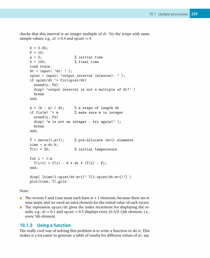
10.1 Update processes 239
checks that this interval is an integer multiple of dt . Try the script with samesample values, e.g., dt = 0.4 and opint = 4.
K = 0.05;F = 10;a = 0; % initial timeb = 100; % final timeload traindt = input( ’dt: ’ );opint = input( ’output interval (minutes): ’ );if opint/dt ~= fix(opint/dt)
sound(y, Fs)disp( ’output interval is not a multiple of dt!’ )break
end;
m = (b - a) / dt; % m steps of length dtif fix(m) ~= m % make sure m is integer
sound(y, Fs)disp( ’m is not an integer - try again!’ );break
end;
T = zeros(1,m+1); % pre-allocate (m+1) elementstime = a:dt:b;T(1) = 25; % initial temperature
for i = 1:mT(i+1) = T(i) - K * dt * (T(i) - F);
end;
disp( [time(1:opint/dt:m+1)’ T(1:opint/dt:m+1)’] )plot(time, T),grid
Note:
� The vectors T and time must each have m+ 1 elements, because there are m
time steps, and we need an extra element for the initial value of each vector.� The expression opint/dt gives the index increment for displaying the re-
sults, e.g., dt = 0.1 and opint= 0.5 displays every (0.5/0.1)th element, i.e.,every 5th element.
10.1.3 Using a functionThe really cool way of solving this problem is to write a function to do it. Thismakes it a lot easier to generate a table of results for different values of dt , say,
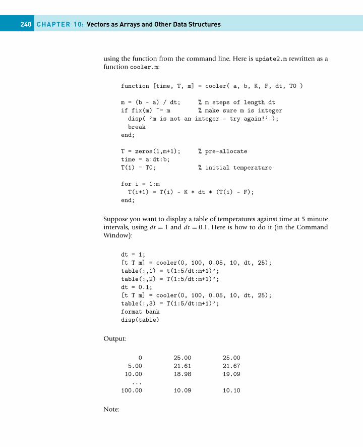
240 CHAPTER 10: Vectors as Arrays and Other Data Structures
using the function from the command line. Here is update2.m rewritten as afunction cooler.m:
function [time, T, m] = cooler( a, b, K, F, dt, T0 )
m = (b - a) / dt; % m steps of length dtif fix(m) ~= m % make sure m is integer
disp( ’m is not an integer - try again!’ );break
end;
T = zeros(1,m+1); % pre-allocatetime = a:dt:b;T(1) = T0; % initial temperature
for i = 1:mT(i+1) = T(i) - K * dt * (T(i) - F);
end;
Suppose you want to display a table of temperatures against time at 5 minuteintervals, using dt = 1 and dt = 0.1. Here is how to do it (in the CommandWindow):
dt = 1;[t T m] = cooler(0, 100, 0.05, 10, dt, 25);table(:,1) = t(1:5/dt:m+1)’;table(:,2) = T(1:5/dt:m+1)’;dt = 0.1;[t T m] = cooler(0, 100, 0.05, 10, dt, 25);table(:,3) = T(1:5/dt:m+1)’;format bankdisp(table)
Output:
0 25.00 25.005.00 21.61 21.6710.00 18.98 19.09
...100.00 10.09 10.10
Note:
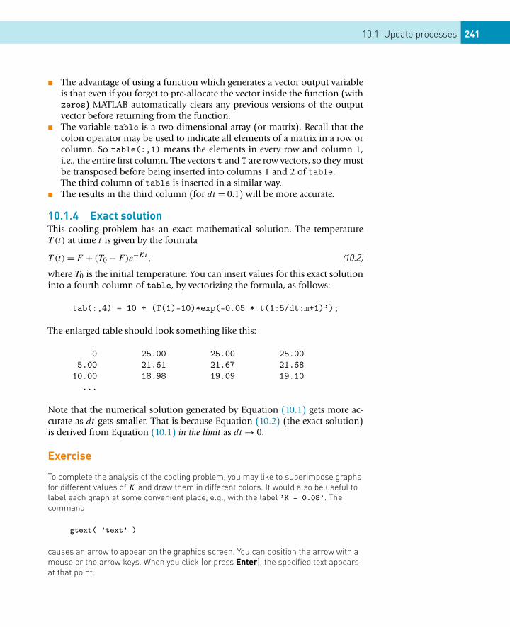
10.1 Update processes 241
� The advantage of using a function which generates a vector output variableis that even if you forget to pre-allocate the vector inside the function (withzeros) MATLAB automatically clears any previous versions of the outputvector before returning from the function.
� The variable table is a two-dimensional array (or matrix). Recall that thecolon operator may be used to indicate all elements of a matrix in a row orcolumn. So table(:,1) means the elements in every row and column 1,i.e., the entire first column. The vectors t and T are row vectors, so they mustbe transposed before being inserted into columns 1 and 2 of table.The third column of table is inserted in a similar way.
� The results in the third column (for dt = 0.1) will be more accurate.
10.1.4 Exact solutionThis cooling problem has an exact mathematical solution. The temperatureT (t) at time t is given by the formula
T (t) = F + (T0 − F)e−Kt , (10.2)
where T0 is the initial temperature. You can insert values for this exact solutioninto a fourth column of table, by vectorizing the formula, as follows:
tab(:,4) = 10 + (T(1)-10)*exp(-0.05 * t(1:5/dt:m+1)’);
The enlarged table should look something like this:
0 25.00 25.00 25.005.00 21.61 21.67 21.68
10.00 18.98 19.09 19.10...
Note that the numerical solution generated by Equation (10.1) gets more ac-curate as dt gets smaller. That is because Equation (10.2) (the exact solution)is derived from Equation (10.1) in the limit as dt → 0.
Exercise
To complete the analysis of the cooling problem, you may like to superimpose graphsfor different values of K and draw them in different colors. It would also be useful tolabel each graph at some convenient place, e.g., with the label ’K = 0.08’. Thecommand
gtext( ’text’ )
causes an arrow to appear on the graphics screen. You can position the arrow with amouse or the arrow keys. When you click (or press Enter), the specified text appearsat that point.
242 CHAPTER 10: Vectors as Arrays and Other Data Structures
The function gtext takes a string argument. If you want to label with a variablenumeric value, use sprintf to convert a number into a string. It works just likefprintf, except that the output goes into a string variable, e.g.,
gtext( sprintf(’K = %5.3f’, K) )
� Draw some graphs, on the same set of axes, for different values of K , in differentcolors, and label them. Figure 10.1 shows what to aim for.Also superimpose the exact solution, given by Equation (10.2).
Plots can also be labeled interactively in plot editing mode or with the Properties Edi-tor.
10.2 FREQUENCIES, BAR CHARTS AND HISTOGRAMS
10.2.1 A random walkImagine an ant walking along a straight line, e.g., the x-axis. She starts at x = 40.She moves in steps of one unit along the line. Each step is to the left or the rightwith equal probability. We would like a visual representation of how muchtime she spends at each position.
Start by running the following script, ant.m:
f = zeros(1,100);x = 40;
for i = 1:1000r = rand;if r >= 0.5
x = x + 1;else
x = x - 1;endif x ~= 0 | x ~= 100
f(x) = f(x) + 1;end
end
Now enter the statement bar(f) in the Command Window. You should get agraph which is similar to the one in Figure 10.2.
Note:
� The function rand returns a random number in the range 0–1. If it’s greaterthan 0.5, the ant moves right (x = x + 1), otherwise she moves left(x = x - 1).
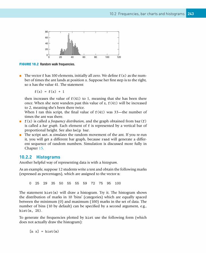
10.2 Frequencies, bar charts and histograms 243
FIGURE 10.2 Random walk frequencies.
� The vector f has 100 elements, initially all zero. We define f(x) as the num-ber of times the ant lands at position x. Suppose her first step is to the right,so x has the value 41. The statement
f(x) = f(x) + 1
then increases the value of f(41) to 1, meaning that she has been thereonce. When she next wanders past this value of x, f(41) will be increasedto 2, meaning she’s been there twice.When I ran this script, the final value of f(41) was 33—the number oftimes the ant was there.
� f(x) is called a frequency distribution, and the graph obtained from bar(f)is called a bar graph. Each element of f is represented by a vertical bar ofproportional height. See also help bar.
� The script ant.m simulates the random movement of the ant. If you re-runit, you will get a different bar graph, because rand will generate a differ-ent sequence of random numbers. Simulation is discussed more fully inChapter 15.
10.2.2 HistogramsAnother helpful way of representing data is with a histogram.
As an example, suppose 12 students write a test and obtain the following marks(expressed as percentages), which are assigned to the vector m:
0 25 29 35 50 55 55 59 72 75 95 100
The statement hist(m) will draw a histogram. Try it. The histogram showsthe distribution of marks in 10 ‘bins’ (categories) which are equally spacedbetween the minimum (0) and maximum (100) marks in the set of data. Thenumber of bins (10 by default) can be specified by a second argument, e.g.,hist(m, 25).
To generate the frequencies plotted by hist use the following form (whichdoes not actually draw the histogram):
[n x] = hist(m)
244 CHAPTER 10: Vectors as Arrays and Other Data Structures
n is a vector containing the frequencies, viz.,
1 0 2 1 0 4 0 2 0 1 1
For example, there is one mark in the first bin (0–9), none in the second (10–19), two in the third, etc.
The second output vector x contains the midpoints of the bins, such thatbar(x, n) plots the histogram. See Help for more details.
Note the subtle difference between a histogram and a bar graph. The valuesplotted by hist are computed from the distribution of values in a vector,whereas bar generates a bar graph directly from the values themselves.
10.3 SORTING
One of the standard applications of arrays is sorting a list of numbers into, say,ascending order. Although MATLAB has its own sorting function (sort), youmay be interested in how sorting algorithms actually work.
10.3.1 Bubble SortThe basic idea is that the unsorted list is assigned to a vector. The numbers arethen ordered by a process which essentially passes through the vector manytimes, swopping consecutive elements that are in the wrong order, until all theelements are in the right order. Such a process is called a Bubble Sort, becausethe smaller numbers rise to the top of the list, like bubbles of air in water. (Infact, in the version shown below, the largest number will ‘sink’ to the bottomof the list after the first pass, which really makes it a ‘Lead Ball’ sort.) There aremany other methods of sorting, such as the Quick Sort, which may be found inmost textbooks on computer science. These are generally more efficient thanthe Bubble Sort, but its advantage is that it is by far the easiest method toprogram. A structure plan for the Bubble Sort is as follows:
1. Input the list X
2. Set N to the length of X
3. Repeat N − 1 times with counter K :Repeat N − K times with counter J :
If Xj > Xj+1 thenSwop the contents of Xj and Xj+1
4. Stop since the list X is now sorted.
As an example, consider a list of five numbers: 27, 13, 9, 5 and 3. They areinitially input into the vector X. Part of MATLAB’s memory for this problem issketched in Table 10.1. Each column shows the list during each pass. A strokein a row indicates a change in that variable during the pass as the script worksdown the list. The number of tests (Xj > Xj+1?) made on each pass is also
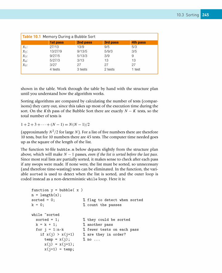
10.3 Sorting 245
Table 10.1 Memory During a Bubble Sort1st pass 2nd pass 3rd pass 4th pass
X1: 27/13 13/9 9/5 5/3X2: 13/27/9 9/13/5 5/9/3 3/5X3: 9/27/5 5/13/3 3/9 9X4: 5/27/3 3/13 13 13X5: 3/27 27 27 27
4 tests 3 tests 2 tests 1 test
shown in the table. Work through the table by hand with the structure planuntil you understand how the algorithm works.
Sorting algorithms are compared by calculating the number of tests (compar-isons) they carry out, since this takes up most of the execution time during thesort. On the Kth pass of the Bubble Sort there are exactly N − K tests, so thetotal number of tests is
1 + 2 + 3 + · · · + (N − 1) = N(N − 1)/2
(approximately N2/2 for large N). For a list of five numbers there are therefore10 tests, but for 10 numbers there are 45 tests. The computer time needed goesup as the square of the length of the list.
The function M-file bubble.m below departs slightly from the structure planabove, which will make N − 1 passes, even if the list is sorted before the last pass.Since most real lists are partially sorted, it makes sense to check after each passif any swops were made. If none were, the list must be sorted, so unnecessary(and therefore time-wasting) tests can be eliminated. In the function, the vari-able sorted is used to detect when the list is sorted, and the outer loop iscoded instead as a non-deterministic while loop. Here it is:
function y = bubble( x )n = length(x);sorted = 0; % flag to detect when sortedk = 0; % count the passes
while ~sortedsorted = 1; % they could be sortedk = k + 1; % another passfor j = 1:n-k % fewer tests on each pass
if x(j) > x(j+1) % are they in order?temp = x(j); % no ...x(j) = x(j+1);x(j+1) = temp;
246 CHAPTER 10: Vectors as Arrays and Other Data Structures
sorted = 0; % a swop was madeend
endend;
y = x;
You can test it on the command line to sort say 20 random numbers as follows:
r = rand(1,20);r = bubble( r );
Note how bubble changes its input vector.
On my PC bubble takes 1.81 s to sort 200 random numbers, but 7.31 s to sort400 numbers. This is consistent with the theoretical result obtained above.
10.3.2 MATLAB’s sortThe built-in MATLAB function sort returns two output arguments: the sortedlist (in ascending order) and a vector containing the indexes used in the sort,i.e., the positions of the sorted numbers in the original list. If the randomnumbers
r = 0.4175 0.6868 0.5890 0.9304 0.8462
are sorted with the command
[y,i] = sort(r)
the output variables are
y = 0.4175 0.5890 0.6868 0.8462 0.9304i = 1 3 2 5 4
For example, the index of the second largest number (0.5890) is 3, which is itssubscript in the original unsorted list r.
As a matter of fact, the built-in functions max and min also return second outputvariables giving indexes.
MATLAB’s sort is very fast. My PC takes 2.36 s to sort a list of one millionrandom numbers! This is because (a) a Quick Sort is used, and (b) the scripthas been compiled as a built-in function; this makes for faster code.
10.4 Structures 247
10.4 STRUCTURES
Up to now we have seen arrays with only one type of element—all numeric,or all character. A MATLAB structure allows you to put different kinds of datain its various fields. For example, we can create a structure called student withone field for a student’s name,
student.name = ’Thandi Mangwane’;
a second field for her student ID number,
student.id = ’MNGTHA003’;
and a third field for all her marks to date,
student.marks = [36 49 74];
To see the whole structure, enter its name:
student
student =name: ’Thandi Mangwane’
id: ’MNGTHA003’marks: [36 49 74]
Here’s how to access her second mark:
student.marks(2)ans =
49
Note the use of the dot to separate the structure name from its fields whencreating it and when accessing its fields.
To add further elements to the structure, use subscripts after the structure name:
student(2).name = ’Charles Wilson’student(2).id = ’WLSCHA007’student(2).marks = [49 98]
(the original student, Thandi Mangwane, is now accessed as student(1)).Note that field sizes do not have to conform across elements of a structure
248 CHAPTER 10: Vectors as Arrays and Other Data Structures
array: student(1).marks has three elements, while student(2).marks hasonly two elements.
The student structure now has size 1-by-2: it has two elements, each elementbeing a student with three fields. Once a structure has more than one elementMATLAB does not display the contents of each field when you type the struc-ture name at the command line. Instead, it gives the following summary:
student
student =1x2 struct array with fields:
nameidmarks
You can also use fieldnames(student) to get this information.
A structure array can be preallocated with the struct function. See Help.
A structure field can contain any kind of data, even another structure—whyever not? Thus we can create a structure course of courses taken by students,where one field is the name of the course, and another field is a student struc-ture with information on all the students taking that particular course:
course.name = ’MTH101’;course.class = student;course
course =name: ’MTH101’
class: [1x2 struct]
We can set up a second element of course for a different class of students:
course(2).name = ’PHY102’;course(2).class = ...
To see all the courses:
course(1:2).nameans =MTH101ans =PHY102
10.5 Cell arrays 249
To see all the students in a particular course:
course(1).class(1:2).nameans =Thandi Mangwaneans =Charles Wilson
There is a curious function called deal which ‘deals inputs to outputs’. You canuse it to generate ‘comma-separated variable lists’ from structure fields:
[name1, name2] = deal(course(1).class(1:2).name);
(but you don’t actually need the commas here . . . ).
You can use the rmfield function to remove fields from a structure.
10.5 CELL ARRAYS
A cell is the most general data object in MATLAB. A cell may be thought of asa ‘data container’, which can contain any type of data: numeric arrays, strings,structures, or cells. An array of cells (and they almost always occur in arrays) iscalled a cell array. While you might think a cell sounds the same as a structure,a cell is more general, and there are also notational differences (which areconfusing!).
10.5.1 Assigning data to cell arraysThere are a number of ways of assigning data to cell arrays.
� Cell indexing:
c(1,1) = {rand(3)};c(1,2) = {char(’Bongani’, ’Thandeka’)};c(2,1) = {13};c(2,2) = {student};
c =[3x3 double] [2x8 char ][ 13] [1x2 struct]
(assuming that the structure student created above still exists). Here theround brackets on the left-hand side of the assignments refer in the normalway to the elements of the cell array. What is different are the curly braceson the right. Curly braces indicate the contents of a cell; on the right-handside of an assignment they are technically cell array constructors (rememberthat each element of this array is a cell).
250 CHAPTER 10: Vectors as Arrays and Other Data Structures
So read the first statement as
‘Construct a cell containing rand(3) and assign the cell to element 1,1 ofthe cell array c.’
� Content indexing:
c{1,1} = rand(3);c{1,2} = char(’Bongani’, ’Thandeka’);c{2,1} = 13;c{2,2} = student;
Here the curly braces on the left indicate the contents of the cell element atthat particular location. So read the first statement as
‘The contents of the cell at location 1,1 becomes rand(3).’
� You can use the curly braces to construct an entire cell array in one state-ment:
b = {[1:5], rand(2); student, char(’Jason’, ’Amy’)}b =
[1x5 double] [2x2 double][1x2 struct] [2x5 char ]
A cell may contain another cell array; nested curly braces may be used tocreate nested cell arrays.
� The cell function enables you to preallocate empty cell arrays, e.g.
a = cell(3,2) % empty 3-by-2 cell arraya =
[] [][] [][] []
You can then use assignment statements to fill the cells, e.g.
a(2,2) = {magic(3)}
Note: if you already have a numeric array with a certain name, don’t try tocreate a cell array of the same name by assignment without first clearing thenumeric array. If you don’t clear the numeric array, MATLAB will generate anerror (it will think you are trying to mix cell and numeric syntaxes).
10.5.2 Accessing data in cell arraysYou can access cell contents using content indexing (curly braces):
r = c{1,1}r =
0.4447 0.9218 0.40570.6154 0.7382 0.93550.7919 0.1763 0.9169
10.5 Cell arrays 251
To access a subset of a cell’s contents you can concatenate curly braces andround brackets if necessary:
rnum = c{1,1}(2,3)rnum =
0.9355
Here the curly braces (content indexing) indicate the contents of the cell arrayelement c(1,1), which is a 3-by-3 numeric matrix. The subscripts (2,3) thenindicate the appropriate element within the matrix.
Curly braces may be concatenated to access nested cell arrays.
10.5.3 Using cell arraysCell arrays come into their own when you need to access (different types of)data as ‘comma-separated variable lists’, as the next example demonstrates.
The functions varargin and varargout, which allow a function to have anynumber of input or output arguments, are none other than cell arrays. Thefunction testvar has a variable number of input arguments, which are dou-bled into the variable number of output arguments (assuming that the numberof output arguments does not exceed the number of input arguments):
function [varargout] = testvar(varargin)
for i = 1:length(varargin)x(i) = varargin{i}; % unpack the input args
end
for i = 1:nargout % how many output arguments?varargout{i} = 2*x(i); % pack up the output args
end
Command line:
[a b c] = testvar(1, 2, 3, 4)a =
2b =
4c =
6
When a function is called with the input argument varargin MATLAB auto-matically packs the list of corresponding input arguments into a cell array. You
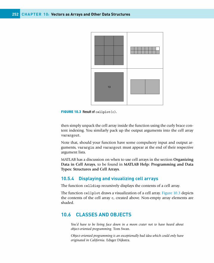
252 CHAPTER 10: Vectors as Arrays and Other Data Structures
FIGURE 10.3 Result of cellplot(c).
then simply unpack the cell array inside the function using the curly brace con-tent indexing. You similarly pack up the output arguments into the cell arrayvarargout.
Note that, should your function have some compulsory input and output ar-guments, varargin and varargout must appear at the end of their respectiveargument lists.
MATLAB has a discussion on when to use cell arrays in the section OrganizingData in Cell Arrays, to be found in MATLAB Help: Programming and DataTypes: Structures and Cell Arrays.
10.5.4 Displaying and visualizing cell arraysThe function celldisp recursively displays the contents of a cell array.
The function cellplot draws a visualization of a cell array. Figure 10.3 depictsthe contents of the cell array c, created above. Non-empty array elements areshaded.
10.6 CLASSES AND OBJECTS
You’d have to be living face down in a moon crater not to have heard aboutobject-oriented programming. Tom Swan.
Object-oriented programming is an exceptionally bad idea which could only haveoriginated in California. Edsger Dijkstra.
10.6 Summary 253
MATLAB, along with most other modern programming languages, espousesthe cause of object-oriented programming, and has all the usual parapherna-lia associated with this paradigm: classes, objects, encapsulation, inheritance,operator overloading, etc., etc.
Object-oriented programming is a subject which requires an entire book todo justice to it. If you want to learn about the concepts, there are many ex-cellent books on the subject. If you want to see how MATLAB implementsobject-oriented programming, consult the online Help: MATLAB Help: Pro-gramming and Data Types: MATLAB Classes and Objects.
SUMMARY� A MATLAB structure allows you to store different types of data in its various
fields.� Arrays of structures may be created.� A cell is the most general data object in MATLAB, and can store any type of
data.� An array of cells is called a cell array—each cell in the array can store differ-
ent types of data, including other cell arrays.� A cell array is constructed with curly braces {}.� The contents of cell in a cell array is accessed with content indexing (curly
braces).� Cell elements in a cell array are accessed in the usual way with round brack-
ets (cell indexing).� Arguments of functions using a variable number of arguments are packed
into cell arrays.� The function cellplot gives a visualization of a cell array.� MATLAB implements object-oriented programming.
CONTENTS
Syntax errors ..... 255Incompatible vectorsizes ...................... 256Name hiding .......... 256
Logic errors ....... 256
Rounding error.. 257
Summary ............ 258
Chapterexercises............. 258
CHAPTER 11
Errors and Pitfalls
THE OBJECTIVE OF THIS CHAPTER IS TO ENABLE YOU TO:
� Begin to recognize and avoid different sorts of errors and pitfalls.
Even experienced programmers seldom get programs to run correctly the firsttime. In computer jargon, an error in a program is called a bug. The story isthat a hapless moth short-circuited two thermionic valves in one of the earliestcomputers. This primeval (charcoaled) ‘bug’ took days to find. The process ofdetecting and correcting such errors is therefore called debugging. There are anumber of different types of errors and pitfalls, some of which are peculiar toMATLAB, and some of which may occur when programming in any language.These are discussed briefly in this chapter.
11.1 SYNTAX ERRORS
Syntax errors are typing errors in MATLAB statements (e.g., plog instead ofplot). They are the most frequent type of error, and are fatal: MATLAB stopsexecution and displays an error message. As MATLAB evolves from one versionto the next, error messages improve. Try the following examples to examinethe latest error messages:
2*(1+3
disp([’the answer is ’ num2str(2)]
There are many possible syntax errors—you will probably have discovered afew yourself. With experience you will become more adept at spotting yourmistakes.
The function lasterr returns the last error message generated.255
Essential MATLAB for Engineers and Scientists. DOI:10.1016/B978-0-08-100877-5.00012-8Copyright © 2017 Daniel T. Valentine. Published by Elsevier Ltd. All rights reserved.
256 CHAPTER 11: Errors and Pitfalls
11.1.1 Incompatible vector sizesConsider the following statements:
x = 0:pi/20:3*pi;y = sin(x);x = 0:pi/40:3*pi;plot(x,y)
You’ll get the error message
Error using ==> plotVectors must be the same lengths.
because you forgot to recalculate y after reducing the x increments. whos revealsthe problem:
x 1x121 ...y 1x61 ...
11.1.2 Name hidingRecall that a workspace variable ‘hides’ a script or function of the same name.The only way to access such a script or function is to clear the offending vari-able from the workspace.
Furthermore, a MATLAB function hides a script of the same name, e.g., create ascript called why.m that displays some junk message, and then type why at thecommand line.
If you are worried that a variable or script which you are thinking of creating,say blob, may be a MATLAB function, try help blob first.
11.2 LOGIC ERRORS
These are errors in the actual algorithm you are using to solve a problem, andare the most difficult to find; the program runs, but gives the wrong answers!It’s even worse if you don’t realize the answers are wrong. The following tipsmight help you to check out the logic.
� Try to run the program for some special cases where you know the answers.� If you don’t know any exact answers, try to use your insight into the prob-
lem to check whether the answers seem to be of the right order of magni-tude.
� Try working through the program by hand (or use MATLAB’s excellent in-teractive debugging facilities—see Chapter 7) to see if you can spot wherethings start going wrong.
11.3 Rounding error 257
11.3 ROUNDING ERROR
At times, as we have seen, a program will give numerical answers which weknow are wrong. This can also be due to rounding error, which results from thefinite precision available on the computer, i.e., eight bytes per variable, insteadof an infinite number.
Run the following program:
x = 0.1;while x ~= 0.2
x = x + 0.001;fprintf( ’%g %g\n’, x, x - 0.2 )
end
You will find that you need to crash the program to stop it, i.e., with Ctrl-breakon a PC. The variable x never has the value 0.2 exactly, because of roundingerror. In fact, x misses 0.2 by about 8.3 × 10⁻¹⁷, as can be seen from displayingthe value of x - 0.2. It would be better to replace the while clause with
while x <= 0.2
or, even better, with
while abs(x - 0.2) > 1e-6
In general, it is always better to test for ‘equality’ of two non-integer expressionsas follows:
if abs((a-b)/a) < 1e-6 disp( ’a practically equals b’ ),end
or
if abs((a-b)/b) < 1e-6 ...
Note that this equality test is based on the relative difference between a and b,rather than on the absolute difference.
Rounding error may sometimes be reduced by a mathematical re-arrangementof a formula. Recall yet again the common or garden quadratic equation
ax2 + bx + c = 0,
with solutions
258 CHAPTER 11: Errors and Pitfalls
x1 = (−b +√
b2 − 4ac)/(2a),
x2 = (−b −√
b2 − 4ac)/(2a).
Taking a = 1, b = −107 and c = 0.001 gives x1 = 107 and x2 = 0. The secondroot is expressed as the difference between two nearly equal numbers, and con-siderable significance is lost. However, as you no doubt remember, the productof the two roots is given by c/a. The second root can therefore be expressed as(c/a)/x1. Using this form gives x2 = 10−10, which is more accurate.
SUMMARY� Syntax errors are mistakes in the construction of MATLAB statements.� Logical errors are errors in the algorithm used to solve a problem.� Rounding error occurs because a computer can store numbers only to a
finite accuracy.
CHAPTER EXERCISES11.1 The Newton quotient
f (x + h) − f (x)
h
may be used to estimate the first derivative f ′(x) of a function f (x), if h is‘small’. Write a program to compute the Newton quotient for the function
f (x) = x2
at the point x = 2 (the exact answer is 4) for values of h starting at 1,and decreasing by a factor of 10 each time (use a for loop). The effect ofrounding error becomes apparent when h gets ‘too small’, i.e., less thanabout 10−12.
11.2 The solution of the set of simultaneous equations
ax + by = c
dx + ey = f
(Exercise 3.6) is given by
x = (ce − bf )/(ae − bd),
y = (af − cd)/(ae − bd).
If (ae − bd) is small, rounding error may cause quite large inaccuracies inthe solution. Consider the system
0.2038x + 0.1218y = 0.2014,
0.4071x + 0.2436y = 0.4038.
11.3 Chapter exercises 259
Show that with four-figure floating point arithmetic the solution ob-tained is x = −1, y = 3. This level of accuracy may be simulated in thesolution of Exercise 3.6 with some statements like
ae = floor( a * e * 1e4 ) / 1e4
and appropriate changes in the coding. The exact solution, obtained with-out rounding, is x = −2, y = 5. If the coefficients in the equations arethemselves subject to experimental error, the ‘solution’ of this system us-ing limited accuracy is totally meaningless.
2P A R T
Applications
Part 2 is on applications. Since this is an introductory course, the applicationsare not extensive. They are illustrative. You ought to recognize that the kindsof problems you actually can solve with MATLAB are much more challengingthan the examples provided. However, many of the examples can be a startingpoint for the development of solutions to more challenging problems. Thegoal of this part of the text is to begin to scratch the surface of the true powerof MATLAB.
CONTENTS
Cantilever beam 265
Electric current . 266
Free fall............... 269
Projectile withfriction ................. 278
Summary ............ 281
Exercises ............ 282
CHAPTER 12
Dynamical Systems
The objective of this chapter is to discuss the importance of learning to usetools like MATLAB. MATLAB and companion toolboxes provide engineers, scien-tists, mathematicians, and students of these fields with an environment for tech-nical computing applications. It is much more than a programming languagelike C, C++ or Fortran. Technical computing includes mathematical computa-tion, analysis, visualization, and algorithm development. The MathWork web-site describes “The Power of Technical Computing with MATLAB” as follows:
� Whatever the objective of your work—an algorithm, an analysis, a graph,a report, or a software simulation—technical computing with MATLAB letsyou work more effectively and efficiently. The flexible MATLABenvironment lets you perform advanced analyses, visualize data, anddevelop algorithms by applying the wealth of functionality available. Withits more than 1000 mathematical, statistical, scientific and engineeringfunctions, MATLAB gives you immediate access to high-performancenumerical computing. This functionality is extended with interactivegraphical capabilities for creating plots, images, surfaces, and volumetricrepresentations.
� The advanced toolbox algorithms enhance MATLAB’s functionality indomains such as signal and image processing, data analysis and statistics,mathematical modeling, and control design. Toolboxes are collections ofalgorithms, written by experts in their fields, that provideapplication-specific numerical, analysis, and graphical capabilities. Byrelying on the work of these experts, you can compare and apply a numberof techniques without writing code. As with MATLAB algorithms, you cancustomize and optimize toolbox functions for your project requirements.
In this chapter we are going to examine the application of MATLAB capabili-ties with four relatively simple problems in engineering science. The problemsare the deflection of a cantilever beam subject to a uniform load, a single-
263Essential MATLAB for Engineers and Scientists. DOI:10.1016/B978-0-08-100877-5.00014-1Copyright © 2017 Daniel T. Valentine. Published by Elsevier Ltd. All rights reserved.
264 CHAPTER 12: Dynamical Systems
loop closed electrical circuit, the free fall problem, and an extension of theprojectile problem discussed in Chapter 2. The first problem is on a structuralelement you investigate in a first course in engineering mechanics. The struc-tural element is the cantilever beam, which is one of the primary elements ofengineered structures, e.g., buildings and bridges. We examine the deflection ofthis beam with a constant cross section when subject to a uniform distributionof load, e.g., its own weight.
The second problem is an examination of the equation that describes the“flow” of electrical current in a simple closed-loop electrical circuit. You ex-amine this type of problem in a first course in electrical science.
The third problem is the free fall of an object in a gravitational field with con-stant acceleration, g. This is one of the first problems you examine in a firstcourse in physics. We examine the effect of friction on the free-fall problemand, hence, learn that with friction (i.e., air resistance) the object can reach aterminal velocity.
The fourth problem is an extension of the projectile that takes into account airresistance (you learn about air resistance in your first course in fluid mechan-ics). By an examination of this problem, you will learn why golfers do not hitthe ball from the tee at 45◦ from the horizontal (which is the optimum anglefor the furthest distance of travel of a projectile launched in frictionless air).
Before we begin, you must keep in mind that this is not a book on engineeringor science; it is an introduction to the essential elements of MATLAB, a pow-erful technical analysis tool. In this and subsequent chapters you will scratchthe surface of its power by solving some relatively simple problems that youhave encountered or will encounter early in your science or engineering edu-cation. Keep in mind that MATLAB is a tool that can be used for a number ofvery productive purposes. One purpose is to learn how to write programs toinvestigate topics you confront in the classroom. You can extend your knowl-edge of MATLAB by self-learning to apply the utilities and any of the toolboxesthat are available to you to solve technical problems. This tool requires a com-mitment from you to continue to discover and to use the power of the toolas part of your continuing education. Developing high-quality computer pro-grams within the MATLAB environment in order to solve technical problemsrequires that you use the utilities available. If you need to write your own codeyou should, if at all possible, include the utilization of generic solvers of par-ticular types of equations that are available in MATLAB. Of course, to do thisyou need to learn more advanced mathematics, science and engineering. Youwill certainly have the opportunity to do this after freshman year.
As a student majoring in science and engineering you will take at least fivesemesters of mathematics. The fifth course is usually titled Advanced Calcu-lus, Advanced Engineering Mathematics, Applied Mathematics, or Methodsof Mathematical Physics. Topics covered in this course are typically ordinary
12.1 Cantilever beam 265
differential equations, systems of differential equations (including nonlinearsystems), linear algebra (including matrix and vector algebra), vector calculus,Fourier analysis, Laplace transforms, partial differential equations, complexanalysis, numerical methods, optimization, probability and statistics. By click-ing the question mark (?) near the center of the upper-most tool bar in theMATLAB desk top, as you already know, opens the help browser. Scan the top-ics and find utilities and examples of approaches to solve problems in all ofthese subjects and more.
The Control Systems Toolbox is an example of one of the numerous engineer-ing and scientific toolboxes that have been developed to advance the art ofdoing science and engineering. SIMULINK and Symbolics are also very im-portant toolboxes. The latter two are included with your “student version”of MATLAB. One of the big advantages of SIMULINK, in addition to beinga graphical algorithm-development and programming environment, is that itis useful when using the computer to measure, record and access data fromlaboratory experiments or data from industrial-process monitoring systems.Symbolics is very useful because it allows you to do symbolic mathematics,e.g., integrating functions like the ones you integrate in your study of the cal-culus. All of the mathematical subjects investigated by you, as a science orengineering major, are applied in your science and engineering courses. Theyare the same techniques that you will apply as a professional (directly or indi-rectly depending on the software tools available within the organization thatyou are employed). Thus, you can use your own copy of MATLAB to help youunderstand the mathematical and software tools that you are expected to applyin the classroom as well as on the job.
12.1 CANTILEVER BEAM
In this section we want to examine the problem of the cantilever beam. Thebeam and its deflection under load is illustrated in Figure 12.1 below, whichis generated by the script m-file created to solve the problem posed next.Many structural mechanics formulas are available in Formulas for Stress andStrain, Fifth Edition by Raymond J. Roark and Warren C. Young, published byMcGraw-Hill Book Company (1982). For a uniformly loaded span of a can-tilever beam attached to a wall at x = 0 with the free end at x = L, the formulafor the vertical displacement from y = 0 under the loaded condition with y thecoordinate in the direction opposite that of the load can be written as follows:
Y = y 24EI
wL4= −
(X4 − 4X3 + 6X2
),
where X = x/L, E is a material property known as the modulus of elastic-ity, I is a geometric property of the cross-section of the beam known as themoment of inertia, L is the length of the beam extending from the wall fromwhich it is mounted, and w is the load per unit width of the beam (this is a
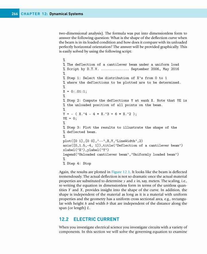
266 CHAPTER 12: Dynamical Systems
two-dimensional analysis). The formula was put into dimensionless form toanswer the following question: What is the shape of the deflection curve whenthe beam is in its loaded condition and how does it compare with its unloadedperfectly horizontal orientation? The answer will be provided graphically. Thisis easily solved by using the following script:
%% The deflection of a cantilever beam under a uniform load% Script by D.T.V. .............. September 2006, May 2016%% Step 1: Select the distribution of X’s from 0 to 1% where the deflections to be plotted are to be determined.%X = 0:.01:1;%% Step 2: Compute the deflections Y at eaxh X. Note that YE is% the unloaded position of all points on the beam.%Y = - ( X.^4 - 4 * X.^3 + 6 * X.^2 );YE = 0;%% Step 3: Plot the results to illustrate the shape of the% deflected beam.%plot([0 1],[0 0],’--’,X,Y,’LineWidth’,2)axis([0,1.5,-4, 1]),title(’Deflection of a cantilever beam’)xlabel(’X’),ylabel(’Y’)legend(’Unloaded cantilever beam’,’Uniformly loaded beam’)%% Step 4: Stop
Again, the results are plotted in Figure 12.1. It looks like the beam is deflectedtremendously. The actual deflection is not so dramatic once the actual materialproperties are substituted to determine y and x in, say, meters. The scaling, i.e.,re-writing the equation in dimensionless form in terms of the unitless quan-tities Y and X, provides insight into the shape of the curve. In addition, theshape is independent of the material as long as it is a material with uniformproperties and the geometry has a uniform cross sectional area, e.g., rectangu-lar with height h and width b that are independent of the distance along thespan (or length) L.
12.2 ELECTRIC CURRENTWhen you investigate electrical science you investigate circuits with a variety ofcomponents. In this section we will solve the governing equation to examine
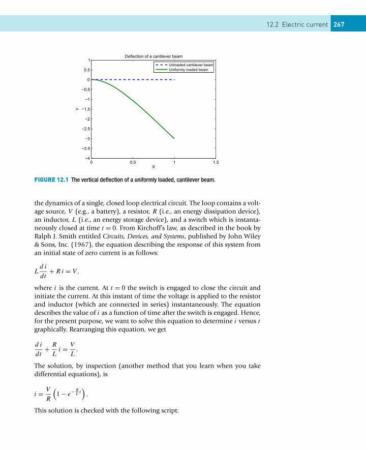
12.2 Electric current 267
FIGURE 12.1 The vertical deflection of a uniformly loaded, cantilever beam.
the dynamics of a single, closed loop electrical circuit. The loop contains a volt-age source, V (e.g., a battery), a resistor, R (i.e., an energy dissipation device),an inductor, L (i.e., an energy storage device), and a switch which is instanta-neously closed at time t = 0. From Kirchoff’s law, as described in the book byRalph J. Smith entitled Circuits, Devices, and Systems, published by John Wiley& Sons, Inc. (1967), the equation describing the response of this system froman initial state of zero current is as follows:
Ld i
dt+ R i = V,
where i is the current. At t = 0 the switch is engaged to close the circuit andinitiate the current. At this instant of time the voltage is applied to the resistorand inductor (which are connected in series) instantaneously. The equationdescribes the value of i as a function of time after the switch is engaged. Hence,for the present purpose, we want to solve this equation to determine i versus t
graphically. Rearranging this equation, we get
d i
dt+ R
Li = V
L.
The solution, by inspection (another method that you learn when you takedifferential equations), is
i = V
R
(1 − e− R
Lt)
.
This solution is checked with the following script:
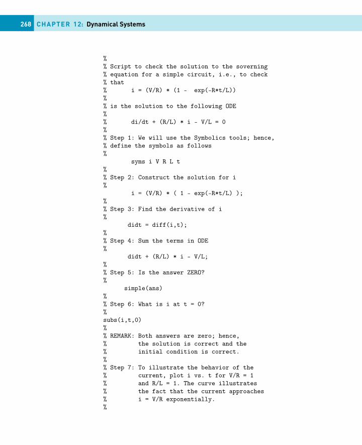
268 CHAPTER 12: Dynamical Systems
%% Script to check the solution to the soverning% equation for a simple circuit, i.e., to check% that% i = (V/R) * (1 - exp(-R*t/L))%% is the solution to the following ODE%% di/dt + (R/L) * i - V/L = 0%% Step 1: We will use the Symbolics tools; hence,% define the symbols as follows%
syms i V R L t%% Step 2: Construct the solution for i%
i = (V/R) * ( 1 - exp(-R*t/L) );%% Step 3: Find the derivative of i%
didt = diff(i,t);%% Step 4: Sum the terms in ODE%
didt + (R/L) * i - V/L;%% Step 5: Is the answer ZERO?%
simple(ans)%% Step 6: What is i at t = 0?%subs(i,t,0)%% REMARK: Both answers are zero; hence,% the solution is correct and the% initial condition is correct.%% Step 7: To illustrate the behavior of the% current, plot i vs. t for V/R = 1% and R/L = 1. The curve illustrates% the fact that the current approaches% i = V/R exponentially.%
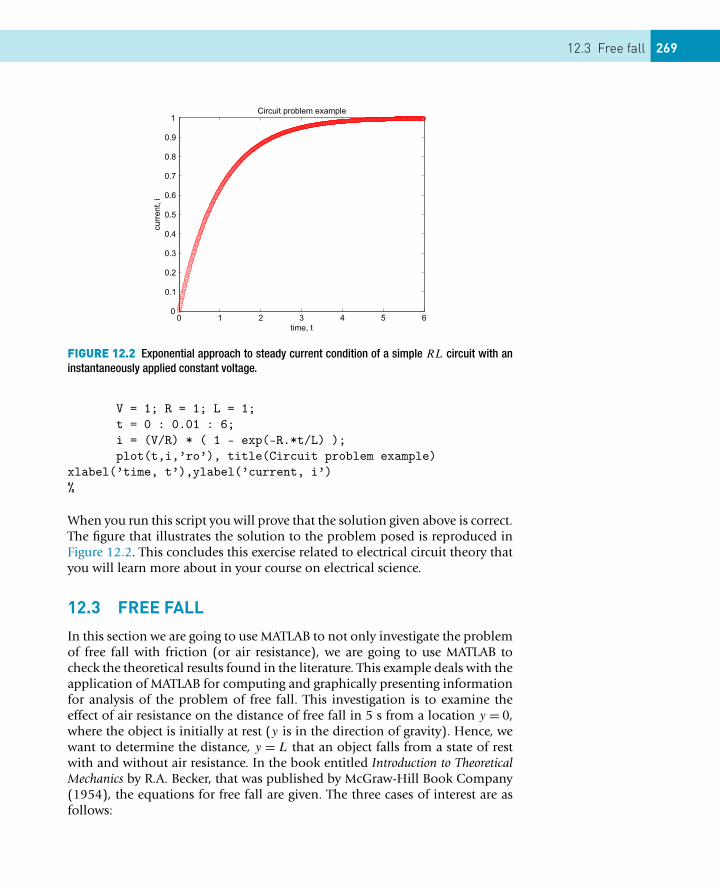
12.3 Free fall 269
FIGURE 12.2 Exponential approach to steady current condition of a simple RL circuit with aninstantaneously applied constant voltage.
V = 1; R = 1; L = 1;t = 0 : 0.01 : 6;i = (V/R) * ( 1 - exp(-R.*t/L) );plot(t,i,’ro’), title(Circuit problem example)
xlabel(’time, t’),ylabel(’current, i’)%
When you run this script you will prove that the solution given above is correct.The figure that illustrates the solution to the problem posed is reproduced inFigure 12.2. This concludes this exercise related to electrical circuit theory thatyou will learn more about in your course on electrical science.
12.3 FREE FALL
In this section we are going to use MATLAB to not only investigate the problemof free fall with friction (or air resistance), we are going to use MATLAB tocheck the theoretical results found in the literature. This example deals with theapplication of MATLAB for computing and graphically presenting informationfor analysis of the problem of free fall. This investigation is to examine theeffect of air resistance on the distance of free fall in 5 s from a location y = 0,where the object is initially at rest (y is in the direction of gravity). Hence, wewant to determine the distance, y = L that an object falls from a state of restwith and without air resistance. In the book entitled Introduction to TheoreticalMechanics by R.A. Becker, that was published by McGraw-Hill Book Company(1954), the equations for free fall are given. The three cases of interest are asfollows:
270 CHAPTER 12: Dynamical Systems
1. Without air resistance:
a = d2y
dt2= g, v = dy
dt= gt, y = 1
2gt2,
where a is the acceleration of the object, v is its speed and y is the distanceof its free fall from the start of motion at t = 0.
2. With resistance proportional to the linear power of velocity:
a = d2y
dt2= g − k
dy
dt, v = dy
dt= g
k
(1 − e−kt
), y = g
kt − g
k2
(1 − e−kt
).
3. With resistance proportional to the second power of velocity:
a = d2y
dt2= g − k
(dy
dt
)2
, v = dy
dt= 1
2
g
ktanh
(gk
2t
),
y = 1
kloge
[cosh (gkt/2)
].
For all three cases the initial condition is y = v = 0 at t = 0. (You will learnmore about ordinary differential equations in your third semester of mathe-matics. In addition, in a first course in fluid mechanics you will learn aboutsome of the details about air resistance. In particular, for air resistance associ-ated with “laminar flow” problems, case 2 applies. In many practical situationsit is case 3 that is usually the case of interest; this is the case where “turbulentflow” is important.)
Let us consider the following problem: Let us assume the above equations arecorrect. Note that they are written for a unit of mass. Let us also assume g =9.81 m/s2 and k = 0.2 for the air-drag parameter. Finally, let us answer thefollowing:
(a) What is y in meters for t = 5 s of free fall for the three cases.(b) What are the terminal speeds in meters per second for cases 2 and 3 for
the specified air-drag parameter?(c) Is the terminal speed reached at t = 5 s?
Note:
The terminal speeds are g/k and (g/k)1/2 for cases 2 and 3, respectively, wherethe terminal speed is the time independent or steady speed reached after asufficient distance of free fall. It is the speed at which the gravitational forcebalances the air resistance force. From Part I, the Essentials, we learned thatMATLAB is quite useful in this type of problem because it has the capability ofcomputing the elementary functions in the formulas above.
As part of providing an answer to the questions raised, we want to examine thedistance of free fall within the 5 s of flight time with the equations for y givenabove. Let us examine the influence of air resistance on free fall graphically;thus, we need to plot the distance y versus t from t = 0 to t = 5 s. We shall plot
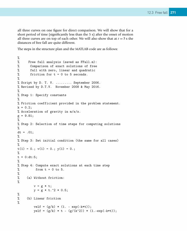
12.3 Free fall 271
all three curves on one figure for direct comparison. We will show that for ashort period of time (significantly less than the 5 s) after the onset of motionall three curves are on top of each other. We will also show that at t = 5 s thedistances of free fall are quite different.
The steps in the structure plan and the MATLAB code are as follows:
%% Free fall analysis (saved as FFall.m):% Comparison of exact solutions of free% fall with zero, linear and quadratic% friction for t = 0 to 5 seconds.%% Script by D. T. V. ......... September 2006.% Revised by D.T.V. November 2008 & May 2016.%% Step 1: Specify constants%% Friction coefficient provided in the problem statement.k = 0.2;% Acceleration of gravity in m/s/s.g = 9.81;%% Step 2: Selection of time steps for computing solutions%dt = .01;%% Step 3: Set initial condition (the same for all cases)%t(1) = 0.; v(1) = 0.; y(1) = 0.;%t = 0:dt:5;%% Step 4: Compute exact solutions at each time step% from t = 0 to 5.%% (a) Without friction:%
v = g * t;y = g * t.^2 * 0.5;
%% (b) Linear friction%
velf = (g/k) * (1. - exp(-k*t));yelf = (g/k) * t - (g/(k^2)) * (1.-exp(-k*t));
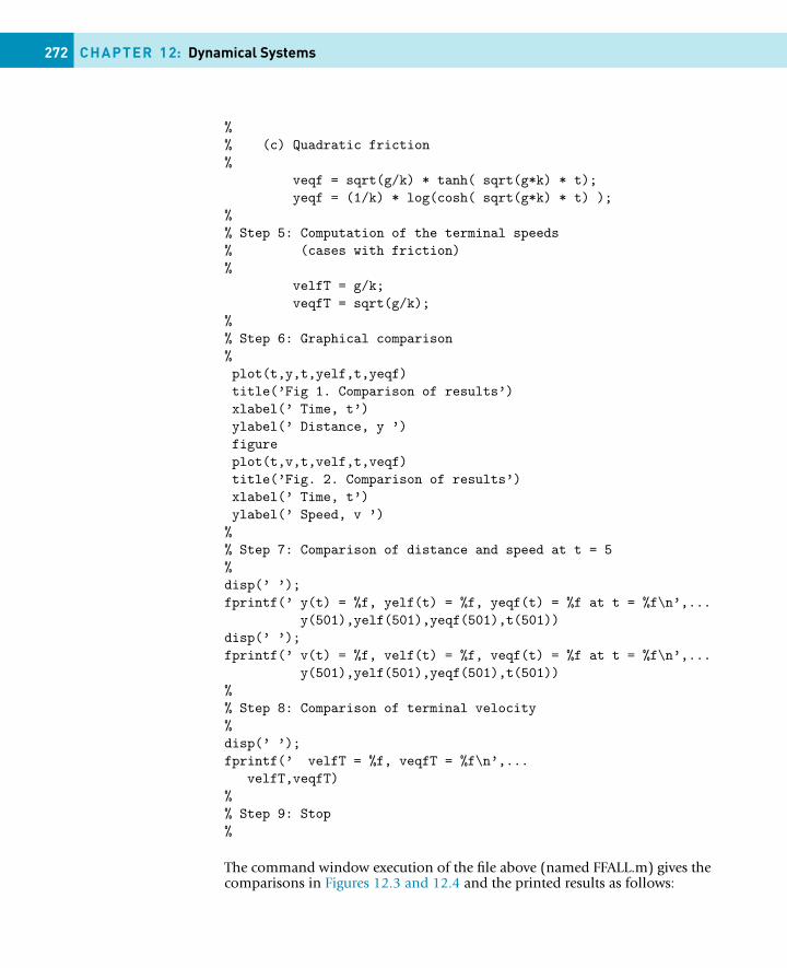
272 CHAPTER 12: Dynamical Systems
%% (c) Quadratic friction%
veqf = sqrt(g/k) * tanh( sqrt(g*k) * t);yeqf = (1/k) * log(cosh( sqrt(g*k) * t) );
%% Step 5: Computation of the terminal speeds% (cases with friction)%
velfT = g/k;veqfT = sqrt(g/k);
%% Step 6: Graphical comparison%plot(t,y,t,yelf,t,yeqf)title(’Fig 1. Comparison of results’)xlabel(’ Time, t’)ylabel(’ Distance, y ’)figureplot(t,v,t,velf,t,veqf)title(’Fig. 2. Comparison of results’)xlabel(’ Time, t’)ylabel(’ Speed, v ’)%% Step 7: Comparison of distance and speed at t = 5%disp(’ ’);fprintf(’ y(t) = %f, yelf(t) = %f, yeqf(t) = %f at t = %f\n’,...
y(501),yelf(501),yeqf(501),t(501))disp(’ ’);fprintf(’ v(t) = %f, velf(t) = %f, veqf(t) = %f at t = %f\n’,...
y(501),yelf(501),yeqf(501),t(501))%% Step 8: Comparison of terminal velocity%disp(’ ’);fprintf(’ velfT = %f, veqfT = %f\n’,...
velfT,veqfT)%% Step 9: Stop%
The command window execution of the file above (named FFALL.m) gives thecomparisons in Figures 12.3 and 12.4 and the printed results as follows:
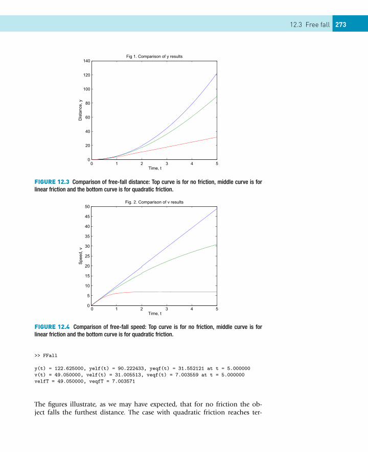
12.3 Free fall 273
FIGURE 12.3 Comparison of free-fall distance: Top curve is for no friction, middle curve is forlinear friction and the bottom curve is for quadratic friction.
FIGURE 12.4 Comparison of free-fall speed: Top curve is for no friction, middle curve is forlinear friction and the bottom curve is for quadratic friction.
>> FFall
y(t) = 122.625000, yelf(t) = 90.222433, yeqf(t) = 31.552121 at t = 5.000000v(t) = 49.050000, velf(t) = 31.005513, veqf(t) = 7.003559 at t = 5.000000velfT = 49.050000, veqfT = 7.003571
The figures illustrate, as we may have expected, that for no friction the ob-ject falls the furthest distance. The case with quadratic friction reaches ter-
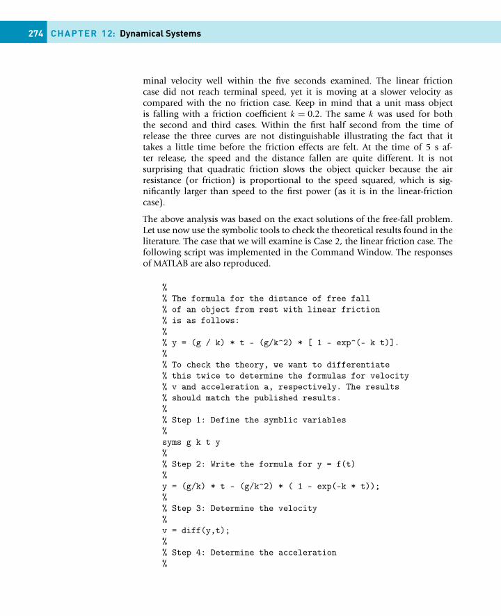
274 CHAPTER 12: Dynamical Systems
minal velocity well within the five seconds examined. The linear frictioncase did not reach terminal speed, yet it is moving at a slower velocity ascompared with the no friction case. Keep in mind that a unit mass objectis falling with a friction coefficient k = 0.2. The same k was used for boththe second and third cases. Within the first half second from the time ofrelease the three curves are not distinguishable illustrating the fact that ittakes a little time before the friction effects are felt. At the time of 5 s af-ter release, the speed and the distance fallen are quite different. It is notsurprising that quadratic friction slows the object quicker because the airresistance (or friction) is proportional to the speed squared, which is sig-nificantly larger than speed to the first power (as it is in the linear-frictioncase).
The above analysis was based on the exact solutions of the free-fall problem.Let use now use the symbolic tools to check the theoretical results found in theliterature. The case that we will examine is Case 2, the linear friction case. Thefollowing script was implemented in the Command Window. The responsesof MATLAB are also reproduced.
%% The formula for the distance of free fall% of an object from rest with linear friction% is as follows:%% y = (g / k) * t - (g/k^2) * [ 1 - exp^(- k t)].%% To check the theory, we want to differentiate% this twice to determine the formulas for velocity% v and acceleration a, respectively. The results% should match the published results.%% Step 1: Define the symblic variables%syms g k t y%% Step 2: Write the formula for y = f(t)%y = (g/k) * t - (g/k^2) * ( 1 - exp(-k * t));%% Step 3: Determine the velocity%v = diff(y,t);%% Step 4: Determine the acceleration%
12.3 Free fall 275
a = diff(v,t);%% Step 5: Print the v and a formulas and compare with% the published results%v, a%% Step 6: Determine a from published formula and v.%a2 = g - k * v;% Step 7: Simplify to somplest forma2 = simple(a2)%% Step 6: Stop. REMARK: Results compare exactly. The% results printed in the command window after executing% this script are as follows:% v = g/k-g/k*exp(-k*t)% a = g*exp(-k*t)% a2 = g/exp(k*t)% These results verify the conclusion that the published% formulas are correct.%
Let us next consider an approximate method for solving the linear-friction case.This procedure is something you could have implemented if you didn’t havethe exact solution. More on numerical methods is provided in Chapter 14 ofthis book.
The equations for free-fall acceleration and velocity are differential equations.The following approximate analysis of a differential equation is called finite-differences. Let us consider the problem of free fall with linear friction (i.e.,air drag that is linearly proportional to the speed of free fall). The formula(or equation) for this problem and its exact solution are given above. In thefollowing analysis a script to solve this problem by the approximate methoddescribed below was written and executed for the same interval of time. Thisis described next. Then the approximate solution is compared with the exactsolution graphically. For a unit mass, the formula that describes the velocityof free fall from rest with air resistance proportional to the linear power ofvelocity can be written as follows:
dv
dt= g − kv.
Let us approximate this equation by inverting the fundamental theorem ofdifferential calculus, i.e., let us re-write it in terms of the definition of what aderivative is before the appropriate limit is taken. What is meant by this is towrite this equation for a small interval of time �t = t (n + 1) − t (n) as follows:
276 CHAPTER 12: Dynamical Systems
dv
dt≈ v(n + 1) − v(n)
�t= g − k
(v(n + 1) + v(n)
2
),
where the value identified by the integer n is the value of v at the beginningof the time interval, i.e., v(n) at t (n). The value identified by n + 1 is the valueof v at the end of the time interval, i.e., v(n + 1) at t (n + 1). This is an initial-value problem; hence, the value of v is known at t (n). Knowing v(n) at t (n),and by specifying t (n + 1), the value v(n + 1) can be calculated by solving thefinite-difference equation for v(n + 1) given above. The solution will dependon the size of �t . This formula gives us v(n + 1). We next need to solve fory(n + 1) from the definition of v (viz., an approximate form of dy/dt). Theaverage value of v over the interval of time, �t , can be written in terms of y asfollows:
dy
dt≈ y(n + 1) − y(n)
�t= v(n + 1) + v(n)
2.
Rearranging this equation, we get a formula for y(n + 1) in terms of v(n + 1),v(n), y(n) and �t . Given the initial condition, i.e., y(n) and v(n) at t (n), wecompute v(n + 1) with the first difference equation followed by computingy(n + 1) with the last equation. Note that the new values become the initial con-dition for the next time step. This procedure is done repeatedly until the overalltime duration of interest is reached (in this case this is t = 5). The script file toimplement this procedure is given next. The m-file is executed and the resultsplotted on the same graph with the exact solution. As shown, the comparisonis remarkable. This is not always the case when approximate methods are used.The comparison is, of course, encouraging because we do not usually have ex-act results and need to resort to numerical approximations in our work.
The script file applied to examine the difference between the approximatemethod and the exact result is as follows:
%% Approximate and exact solution comparison of% free fall with linear friction for t = 0 to 5.%% Script by D. T. V. .......... September 2006.% Revised by D.T.V. . November 2008 & May 2016.%% Step 1: Specified constants%k = 0.2;g = 9.81;%% Step 2: Selection of time step for approximate solution% dt = t(n+1) - t(n)dt = 0.01;
12.3 Free fall 277
%% Step 3: Initial condition%t(1) = 0.;v(1) = 0.;y(1) = 0.;%% Step 3: Sequential implementation of the approximate% solution method by repeating the procedure 500 times% (using a for loop).%for n = 1:1:500
t(n+1) = t(n) + dt;v(n+1) = (v(n) + dt * (g-0.5*k*v(n)) )/(1.+dt*0.5*k);y(n+1) = y(n) + dt * 0.5 * (v(n+1) + v(n));
end%% Step 4: Exact solution over the same interval of time:%
ye = (g/k) * t - (g/(k^2)) * (1.-exp(-k*t));%% Step 5: Graphical comparison:%plot(t,y,’o’,t,ye)title(’Comparison of numerics w/ exact results’)xlabel(’ Time, t’)ylabel(’ Distance of free fall from rest, y’)%% Step 6: Comparison of distance at t=5%disp(’ ’);fprintf(’ y(t) = %f, ye(t) = %f at t = %f \n’,...
y(501),ye(501),t(501))%% Step 7: End of script by DTV.%
In summary, the examination of the free fall problem illustrated the appli-cation and the checking of formulas reported in the literature. In addition,an approximate method was applied to solve the same problem to illustratethe application of a method that would be necessary if exact formulas werenot found. Finally, the approximate method that was applied can certainlybe improved by utilizing the ordinary differential equation solvers available
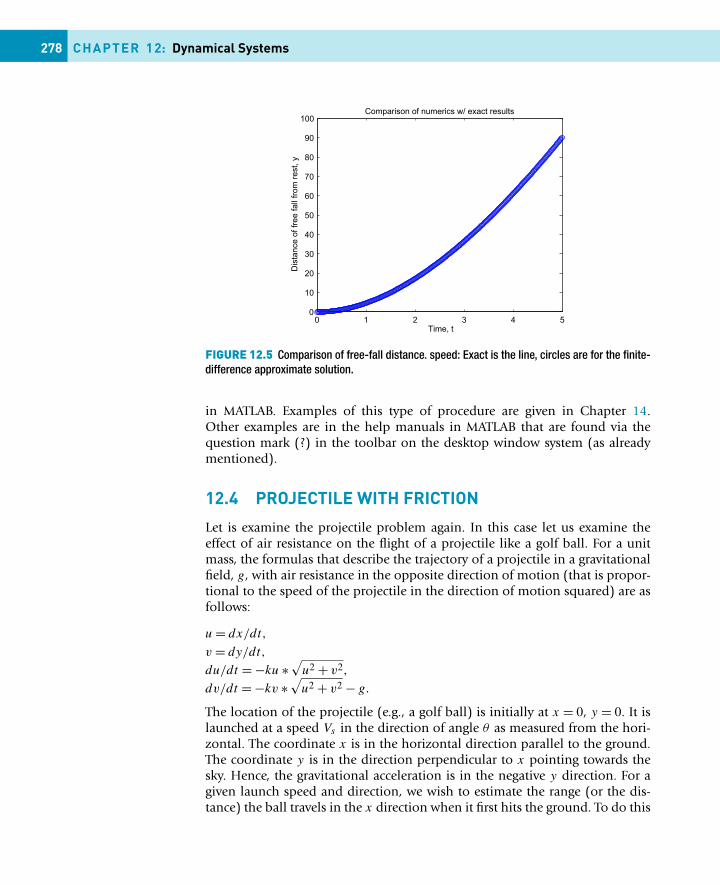
278 CHAPTER 12: Dynamical Systems
FIGURE 12.5 Comparison of free-fall distance. speed: Exact is the line, circles are for the finite-difference approximate solution.
in MATLAB. Examples of this type of procedure are given in Chapter 14.Other examples are in the help manuals in MATLAB that are found via thequestion mark (?) in the toolbar on the desktop window system (as alreadymentioned).
12.4 PROJECTILE WITH FRICTION
Let is examine the projectile problem again. In this case let us examine theeffect of air resistance on the flight of a projectile like a golf ball. For a unitmass, the formulas that describe the trajectory of a projectile in a gravitationalfield, g, with air resistance in the opposite direction of motion (that is propor-tional to the speed of the projectile in the direction of motion squared) are asfollows:
u = dx/dt,
v = dy/dt,
du/dt = −ku ∗√
u2 + v2,
dv/dt = −kv ∗√
u2 + v2 − g.
The location of the projectile (e.g., a golf ball) is initially at x = 0, y = 0. It islaunched at a speed Vs in the direction of angle θ as measured from the hori-zontal. The coordinate x is in the horizontal direction parallel to the ground.The coordinate y is in the direction perpendicular to x pointing towards thesky. Hence, the gravitational acceleration is in the negative y direction. For agiven launch speed and direction, we wish to estimate the range (or the dis-tance) the ball travels in the x direction when it first hits the ground. To do this
12.4 Projectile with friction 279
we shall approximate the four equations in a similar way that we treated thefree falling object problem in the last section.
The solution method is given in detail in the script provided at the end of thisparagraph. It was saved with the name golf.m.
%% "The Golf ball problem"% Numerical computation of the trajectory of a% projectile launched at an angle theta with% a specified launch speed. They are:% theta = launch angle in degrees.% Vs = launch speed.%% Script by D. T. V. ......... September 2006.% Revised by D.T.V. November 2008 & May 2016.%% Equations of motion:% u = dx/dt. v = dy/dt. g is in the opposite% direction of y. x = y = 0 is the location of% the tee. k is the coefficient of air drag. It% is assumed to be constant. Friction is assumed% to be proportional to the speed of the ball% squared and it acts in the opposite direction% of the direction of motion of the ball. The% components of acceleration are thus:% du/dt = - [k (u^2 + v^2) * u/sqrt(u^2+v^2)].% dv/dt = - [k (u^2 + v^2) * v/sqrt(u^2+v^2)] - g.%% INPUT DATA% Specified constants:
k = 0.02;g = 9.81;dt = 0.01;
%% Input the initial condition:%theta = input(’ Initial angle of launch: ’)the = theta * pi/180.;Vs = input(’ Initial speed of launch: ’)u(1) = Vs * cos(the);v(1) = Vs * sin(the);% Launch pad location:x(1) = 0.;y(1) = 0.;
280 CHAPTER 12: Dynamical Systems
%% Compute approximate solution of the trajectory% of flight.% Repeat up to 6000 time, i.e., until ball hits% the ground.%for n=1:1:6000;
u(n+1) = u(n) ...- dt * (k * sqrt(u(n)^2+v(n)^2) * u(n));
v(n+1) = v(n) ...- dt * (k * sqrt(u(n)^2+v(n)^2) * v(n) + g);
x(n+1) = x(n) + u(n) * dt;y(n+1) = y(n) + v(n) * dt;
% Determination of when the object hits ground:if y(n+1) < 0
slope = (y(n+1) - y(n))/(x(n+1) - x(n));b = y(n) - slope * x(n);xhit = - b/slope;
plot(x,y)fprintf(’ The length of the shot = %5.2f \n’, xhit)end
% Once object hits terminate the computations with a break:if y(n+1) < 0; break; end
end%% Graphical presentation of the results:%if y(n+1) > 0
plot(x,y)end% ------ End of golf-ball script by DTV
What is the optimum launch angle for k = 0.02? The answer to this questionis described next for the launch speed of 100. Note that the optimum angleis the angle which gives the longest distance of travel (or greatest range). Tocompute the optimum angle the following script was executed after the lineswith the input statements in the golf.m script were commented out by typing% at the beginning of the two lines with the input commands. The two linesin question were commented out as follows:
%% In golf.m the following alterations were made% prior to running this script!!!!!!%
12.4 Summary 281
% % theta = input(’ Initial angle of launch: ’)% % Vs = input(’ Initial speed of launch: ’)%% This script then finds the optimum angle for k = 0.2% to compare with the zero friction case, which we know% has the optimum launch angle of 45 degrees.%% Script by D. T. V. .......... September 2006.% Revised by D.T.V. November 2008 & May 2016.%% Consider launch angles from 1 to 45 degrees%th = 1:1:45;vs = 100; % Specified launch speed.%% Execute the modified golf.m file 45 times and save% results for each executoion of golf.m%for i=1:45
theta = th(i)golf % Execution of modified golf.m script.xh(i) = xhitthxh(i) = theta
end% Find the maximum distance and the correponding index[xmh,n] = max(xh)% Determine the angle that the maximum distance occured.opt_angle = thxh(n)$ Display the resultsdisp(’ optimum angle ’)disp( opt_angle )% REMARK: For this case the result is 30 degrees.% End of script
The optimum angle of launch for the case of nonlinear friction was computedand found to be equal to 30◦. Without friction it is 45◦. Hence, it is not surpris-ing that golfers launch their best drives at angles significantly less than 45◦.
SUMMARY
In this chapter we examined three problems using some of the utilities in MAT-LAB. We did the following:
282 CHAPTER 12: Dynamical Systems
� We determined the shape of the deflection of a cantilever beam based ona published formula in the engineering literature. Thus, we could use thecapability of MATLAB to do arithmetic with polynomials.
� We examined the effect of friction on the free fall problem. In addition tocomputing the distance and speed of free fall based on published formulas,we checked the formulas with the symbolics tools and we also solved theproblem by an approximate method to illustrate the range of possibilitiesat your disposal to solve technical problems.
� We examined the projectile problem subjected to air resistance. We did thisby applying the same type of approximate method as we applied in thefree fall problem. We found that the optimum angle of launch with frictiontaken into account is less than 45◦ (the frictionless value).
EXERCISES12.1 Reproduce the script for the exact solutions for the free fall problem
(called FFall.m) and execute it for a range of friction coefficients, e.g.,k = 0.1 and 0.3.
12.2 Use the symbolics tools in the same way they were used to check theformulas for the linear-friction case of free fall, to check the other twocases.
12.3 Reproduce the golf.m (projectile script) and look at the effect of varyingthe friction coefficient k. Look at k = 0.01 and 0.03. What influence doesfriction have on the optimum angle for a launch speed of 100?
CONTENTS
Random numbergeneration .......... 283Seeding rand ......... 284
Spinning coins ... 284
Rolling dice ........ 285
Bacteria division286
A random walk .. 286
Traffic flow.......... 288
Normal (Gaussian)randomnumbers ............. 291
Summary ............ 291
Exercises ............ 292
CHAPTER 13
Simulation
THE OBJECTIVE OF THIS CHAPTER IS TO INTRODUCE YOUTO:
� Simulation of “real-life” events.
Simulation is an area of application where computers have come into theirown. A simulation is a computer experiment which mirrors some aspect of thereal world that appears to be based on random processes, or is too compli-cated to understand properly. (Whether events can be really random is actuallya philosophical or theological question.) Some examples are: radio-active de-cay, rolling dice, bacteria division and traffic flow. The essence of a simulationprogram is that the programmer is unable to predict beforehand exactly whatthe outcome of the program will be, which is true to the event being simu-lated. For example, when you spin a coin, you do not know for sure what theresult will be.
13.1 RANDOM NUMBER GENERATION
Random events are easily simulated in MATLAB with the function rand, whichwe have briefly encountered already. By default, rand returns a uniformly dis-tributed pseudo-random number in the range 0 ≤ rand< 1. (A computer cannotgenerate truly random numbers, but they can be practically unpredictable.)rand can also generate row or column vectors, e.g., rand(1,5) returns a rowvector of five random numbers (1 row, 5 column) as shown:
0.9501 0.2311 0.6068 0.4860 0.8913
If you generate more random numbers during the same MATLAB session, youwill get a different sequence each time, as you would expect. However, eachtime you start a MATLAB session, the random number sequence begins at the
283Essential MATLAB for Engineers and Scientists. DOI:10.1016/B978-0-08-100877-5.00015-3Copyright © 2017 Daniel T. Valentine. Published by Elsevier Ltd. All rights reserved.
284 CHAPTER 13: Simulation
same place (0.9501), and continues in the same way. This is not true to life,as every gambler knows. To produce a different sequence each time you start asession, rand can be initially seeded in a different way each time you start.
13.1.1 Seeding randThe random number generator rand can be seeded with the statement
rand(’state’, n)
where n is any integer. (By default, n is set to 0 when a MATLAB session starts.)This is useful if you want to generate the same random sequence every time ascript runs, e.g., in order to debug it properly. Note that this statement doesnot generate any random numbers; it only initializes the generator.
However, you can also arrange for n to be different each time you start MATLABby using the system time. The function clock returns the date and time ina six-element vector with seconds to two decimal places, so the expressionsum(100*clock) never has the same value (well, hardly ever). You can use itto seed rand as follows:
�rand(’state’, sum(100*clock))�rand(1,7)ans =
0.3637 0.2736 0.9910 0.3550 0.8501 0.0911 0.4493�rand(’state’, sum(100*clock))�rand(1,7)ans =
0.9309 0.2064 0.7707 0.7644 0.2286 0.7722 0.5315
Theoretically rand can generate over 21492 numbers before repeating itself.
13.2 SPINNING COINS
When a fair (unbiased) coin is spun, the probability of getting heads or tails is0.5 (50%). Since a value returned by rand is equally likely to anywhere in theinterval (0, 1) we can represent heads, say, with a value less than 0.5, and tailsotherwise.
Suppose an experiment calls for a coin to be spun 50 times, and the resultsrecorded. In real life you may need to repeat such an experiment a number oftimes; this is where computer simulation is handy. The following script simu-lates spinning a coin 50 times:
for i = 1:50
13.3 Rolling dice 285
r = rand;if r < 0.5
fprintf( ’H’ )else
fprintf( ’T’ )end
endfprintf( ’\n’ ) % newline
Here is the output from two sample runs:
THHTTHHHHTTTTTHTHTTTHHTHTTTHHTTTTHTTHHTHHHHHHTTHTTTHTHHHTHTHHTTHTHTTTHHTTTTTTTHHHTTTHTHHTHHHHTTHTHTT
Note that it should be impossible in principle to tell from the output alonewhether the experiment was simulated or real (if the random number genera-tor is sufficiently random).
Can you see why it would be wrong to code the if part of the coin simulationlike this:
if rand < 0.5 fprintf( ’H’ ), endif rand >= 0.5 fprintf( ’T’ ), end
The basic principle is that rand should be called only once for each ‘event’ beingsimulated. Here the single event is spinning a coin, but rand is called twice.Also, since two different random numbers are generated, it is quite possiblethat both logical expressions will be true, in which case ‘H’ and ‘T’ will both bedisplayed for the same coin!
13.3 ROLLING DICE
When a fair dice is rolled, the number uppermost is equally likely to be anyinteger from 1 to 6. We saw in Counting random numbers (Chapter 5) howto use rand to simulate this. The following statement generates a vector with10 random integers in the range 1–6:
d = floor( 6 * rand(1,10) + 1 )
Here are the results of two such simulations:
2 1 5 5 6 3 4 5 1 14 5 1 3 1 3 5 4 6 6
286 CHAPTER 13: Simulation
We can do statistics on our simulated experiment, just as if it were a real one.For example, we could estimate the mean of the number obtained when thedice is rolled 100 times, and the probability of getting a six, say.
13.4 BACTERIA DIVISION
If a fair coin is spun, or a fair dice is rolled, the different events (e.g., getting‘heads’, or a 6) happen with equal likelihood. Suppose, however, that a certaintype of bacteria divides (into two) in a given time interval with a probabilityof 0.75 (75%), and that if it does not divide, it dies. Since a value generatedby rand is equally likely to be anywhere between 0 and 1, the chances of itbeing less than 0.75 are precisely 75%. We can therefore simulate this situationas follows:
r = rand;if r < 0.75
disp( ’I am now we’ )else
disp( ’I am no more’ )end
Again, the basic principle is that one random number should be generated foreach event being simulated. The single event here is the bacterium’s life historyover the time interval.
13.5 A RANDOM WALK
A seriously short-sighted sailor has lost his contact lenses returning from asymphony concert, and has to negotiate a jetty to get to his ship. The jetty is 50paces long and 20 wide. He is in the middle of the jetty at the quay-end, point-ing toward the ship. Suppose at every step he has a 60% chance of stumblingblindly toward the ship, but a 20% chance of lurching to the left or right (hemanages to be always facing the ship). If he reaches the ship-end of the jetty,he is hauled aboard by waiting mates.
The problem is to simulate his progress along the jetty, and to estimate hischances of getting to the ship without falling into the sea. To do this correctly,we must simulate one random walk along the jetty, find out whether or not hereaches the ship, and then repeat this simulation 1000 times, say (if we havea fast enough computer!). The proportion of simulations that end with thesailor safely in the ship will be an estimate of his chances of making it to theship. For a given walk we assume that if he has not either reached the ship orfallen into the sea after, say, 10000 steps, he dies of thirst on the jetty.
13.5 A random walk 287
To represent the jetty, we set up co-ordinates so that the x-axis runs along themiddle of the jetty with the origin at the quay-end. x and y are measured insteps. The sailor starts his walk at the origin each time. The structure plan andscript are as follows:
1. Initialize variables, including number of walks n
2. Repeat n simulated walks down the jetty:Start at the quay-end of the jettyWhile still on the jetty and still alive repeat:
Get a random number R for the next stepIf R < 0.6 then
Move forward (to the ship)Else if R < 0.8 then
Move port (left)Else
Move starboardIf he got to the ship then
Count that walk as a success3. Compute and print estimated probability of reaching the ship4. Stop.
% random walkn = input( ’Number of walks: ’ );nsafe = 0; % number of times he makes it
for i = 1:nsteps = 0; % each new walk ...x = 0; % ... starts at the originy = 0;
while x <= 50 & abs(y) <= 10 & steps < 1000steps = steps + 1; % that’s another stepr = rand; % random number for that stepif r < 0.6 % which way did he go?
x = x + 1; % maybe forward ...elseif r < 0.8
y = y + 1; % ... or to port ...else
y = y - 1; % ... or to starboardend;
end;
if x > 50nsafe = nsafe + 1; % he actually made it this time!
end;
288 CHAPTER 13: Simulation
end;
prob = 100 * nsafe / n;disp( prob );
A sample run of 100 walks gave an 93% probability of reaching the ship.
You can speed up the script by about 20% if you generate a vector of 1 000random numbers, say, at the start of each walk (with r = rand(1,1000);)and then reference elements of the vector in the while loop, e.g.,
if r(steps) < 0.6 ...
13.6 TRAFFIC FLOW
A major application of simulation is in modeling the traffic flow in large cities,in order to test different traffic light patterns before inflicting them on the realtraffic. In this example we look at a very small part of the problem: how tosimulate the flow of a single line of traffic through one set of traffic lights. Wemake the following assumptions (you can make additional or different ones iflike):
1. Traffic travels straight, without turning.2. The probability of a car arriving at the lights in a particular second is in-
dependent of what happened during the previous second. This is called aPoisson process. This probability (call it p) may be estimated by watching carsat the intersection and monitoring their arrival pattern. In this simulationwe take p = 0.3.
3. When the lights are green, assume the cars move through at a steady rateof, say, eight every ten seconds.
4. In the simulation, we will take the basic time period to be ten seconds, sowe want a display showing the length of the queue of traffic (if any) at thelights every ten seconds.
5. We will set the lights red or green for variable multiples of ten seconds.
The situation is modeled with a script file traffic.m which calls three func-tion files: go.m, stop.m, and prq.m. Because the function files need access to anumber of base workspace variables created by traffic.m, these variables aredeclared global in traffic.m, and in all three function files.
In this example the lights are red for 40 s (red = 4) and green for 20 s(green = 2). The simulation runs for 240 s (n = 24).
The script, traffic.m, is as follows:
13.6 Traffic flow 289
clcclear % clear out any previous garbage!global CARS GTIMER GREEN LIGHTS RED RTIMER T
CARS = 0; % number of cars in queueGTIMER = 0; % timer for green lightsGREEN = 2; % period lights are greenLIGHTS = ’R’; % colour of lightsn = 48; % number of 10-sec periodsp = 0.3; % probability of a car arrivingRED = 4; % period lights are redRTIMER = 0; % timer for red lights
for T = 1:n % for each 10-sec period
r = rand(1,10); % 10 seconds means 10 random numbersCARS = CARS + sum(r < p); % cars arriving in 10 seconds
if LIGHTS == ’G’go % handles green lights
elsestop % handles red lights
end;
end;
The function files go.m, stop.m and prq.m (all separate M-files) are as follows:
% ----------------------------------------------------------function goglobal CARS GTIMER GREEN LIGHTSGTIMER = GTIMER + 1; % advance green timerCARS = CARS - 8; % let 8 cars through
if CARS < 0 % ... there may have been < 8CARS = 0;
end;
prq; % display queue of cars
if GTIMER == GREEN % check if lights need to changeLIGHTS = ’R’;GTIMER = 0;
end;
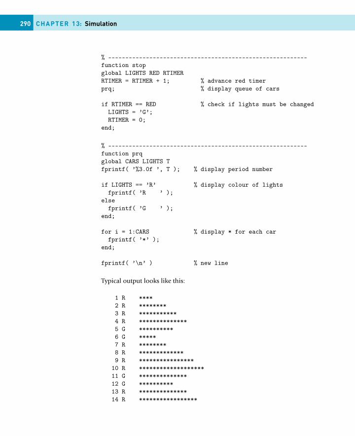
290 CHAPTER 13: Simulation
% ----------------------------------------------------------function stopglobal LIGHTS RED RTIMERRTIMER = RTIMER + 1; % advance red timerprq; % display queue of cars
if RTIMER == RED % check if lights must be changedLIGHTS = ’G’;RTIMER = 0;
end;
% ----------------------------------------------------------function prqglobal CARS LIGHTS Tfprintf( ’%3.0f ’, T ); % display period number
if LIGHTS == ’R’ % display colour of lightsfprintf( ’R ’ );
elsefprintf( ’G ’ );
end;
for i = 1:CARS % display * for each carfprintf( ’*’ );
end;
fprintf( ’\n’ ) % new line
Typical output looks like this:
1 R ****2 R ********3 R ***********4 R **************5 G **********6 G *****7 R ********8 R *************9 R ****************
10 R *******************11 G **************12 G **********13 R **************14 R *****************
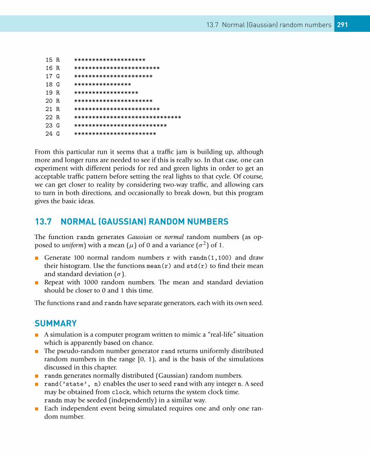
13.7 Normal (Gaussian) random numbers 291
15 R ********************16 R ************************17 G **********************18 G ****************19 R ******************20 R **********************21 R ************************22 R ******************************23 G **************************24 G ***********************
From this particular run it seems that a traffic jam is building up, althoughmore and longer runs are needed to see if this is really so. In that case, one canexperiment with different periods for red and green lights in order to get anacceptable traffic pattern before setting the real lights to that cycle. Of course,we can get closer to reality by considering two-way traffic, and allowing carsto turn in both directions, and occasionally to break down, but this programgives the basic ideas.
13.7 NORMAL (GAUSSIAN) RANDOM NUMBERS
The function randn generates Gaussian or normal random numbers (as op-posed to uniform) with a mean (μ) of 0 and a variance (σ 2) of 1.
� Generate 100 normal random numbers r with randn(1,100) and drawtheir histogram. Use the functions mean(r) and std(r) to find their meanand standard deviation (σ ).
� Repeat with 1000 random numbers. The mean and standard deviationshould be closer to 0 and 1 this time.
The functions rand and randn have separate generators, each with its own seed.
SUMMARY� A simulation is a computer program written to mimic a “real-life” situation
which is apparently based on chance.� The pseudo-random number generator rand returns uniformly distributed
random numbers in the range [0, 1), and is the basis of the simulationsdiscussed in this chapter.
� randn generates normally distributed (Gaussian) random numbers.� rand(’state’, n) enables the user to seed rand with any integer n. A seed
may be obtained from clock, which returns the system clock time.randn may be seeded (independently) in a similar way.
� Each independent event being simulated requires one and only one ran-dom number.
292 CHAPTER 13: Simulation
EXERCISES13.1 Write some statements to simulate spinning a coin 50 times using 0-1
vectors instead of a for loop. Hints: generate a vector of 50 randomnumbers, set up 0-1 vectors to represent the heads and tails, and usedouble and char to display them as a string of Hs and Ts.
13.2 In a game of Bingo the numbers 1 to 99 are drawn at random from abag. Write a script to simulate the draw of the numbers (each numbercan be drawn only once), printing them ten to a line.
13.3 Generate some strings of 80 random alphabetic letters (lowercaseonly). For fun, see how many real words, if any, you can find in thestrings.
13.4 A random number generator can be used to estimate π as follows (sucha method is called a Monte Carlo method). Write a script which gener-ates random points in a square with sides of length 2, say, and whichcounts what proportion of these points falls inside the circle of unitradius that fits exactly into the square. This proportion will be the ratioof the area of the circle to that of the square. Hence estimate π . (This isnot a very efficient method, as you will see from the number of pointsrequired to get even a rough approximation.)
13.5 Write a script to simulate the progress of the short-sighted student inChapter 6 (Markov Processes). Start him at a given intersection, andgenerate a random number to decide whether he moves toward theinternet cafe or home, according to the probabilities in the transitionmatrix. For each simulated walk, record whether he ends up at homeor in the cafe. Repeat a large number of times. The proportion of walksthat end up in either place should approach the limiting probabilitiescomputed using the Markov model described in Chapter 6. Hint: if therandom number is less than 2/3 he moves toward the cafe (unless he isalready at home or in the cafe, in which case that random walk ends),otherwise he moves toward home.
13.6 The aim of this exercise is to simulate bacteria growth.Suppose that a certain type of bacteria divides or dies according to thefollowing assumptions:(a) during a fixed time interval, called a generation, a single bacterium
divides into two identical replicas with probability p;(b) if it does not divide during that interval, it dies;(c) the offspring (called daughters) will divide or die during the next
generation, independently of the past history (there may well beno offspring, in which case the colony becomes extinct).
Start with a single individual and write a script which simulates a num-ber of generations. Take p = 0.75. The number of generations whichyou can simulate will depend on your computer system. Carry out alarge number (e.g. 100) of such simulations. The probability of ultimateextinction, p(E), may be estimated as the proportion of simulations
13.7 Exercises 293
that end in extinction. You can also estimate the mean size of the nthgeneration from a large number of simulations. Compare your estimatewith the theoretical mean of (2p)n.Statistical theory shows that the expected value of the extinction prob-ability p(E) is the smaller of 1, and (1 − p)/p. So for p = 0.75, p(E)
is expected to be 1/3. But for p ≤ 0.5, p(E) is expected to be 1, whichmeans that extinction is certain (a rather unexpected result). You canuse your script to test this theory by running it for different values of p,and estimating p(E) in each case.
13.7 Brian Hahn (the original author of this book) is indebted to a col-league, Gordon Kass, for suggesting this problem.Dribblefire Jets Inc. make two types of aeroplane, the two-engined DFII,and the four-engined DFIV. The engines are terrible and fail with prob-ability 0.5 on a standard flight (the engines fail independently of eachother). The manufacturers claim that the planes can fly if at least halfof their engines are working, i.e. the DFII will crash only if both its en-gines fail, while the DFIV will crash if all four, or if any three enginesfail.You have been commissioned by the Civil Aviation Board to ascer-tain which of the two models is less likely to crash. Since parachutesare expensive, the cheapest (and safest!) way to do this is to simu-late a large number of flights of each model. For example, two calls ofMath.random could represent one standard DFII flight: if both randomnumbers are less than 0.5, that flight crashes, otherwise it doesn’t. Writea script which simulates a large number of flights of both models, andestimates the probability of a crash in each case. If you can run enoughsimulations, you may get a surprising result. (Incidentally, the prob-ability of n engines failing on a given flight is given by the binomialdistribution, but you do not need to use this fact in the simulation.)
13.8 Two players, A and B , play a game called Eights. They take it in turnsto choose a number 1, 2 or 3, which may not be the same as the lastnumber chosen (so if A starts with 2, B may only choose 1 or 3 at thenext move). A starts, and may choose any of the three numbers for thefirst move. After each move, the number chosen is added to a commonrunning total. If the total reaches 8 exactly, the player whose turn itwas wins the game. If a player causes the total to go over 8, the otherplayer wins. For example, suppose A starts with 1 (total 1), B chooses 2(total 3), A chooses 1 (total 4) and B chooses 2 (total 6). A would liketo play 2 now, to win, but he can’t because B cunningly played it onthe last move, so A chooses 1 (total 7). This is even smarter, because B
is forced to play 2 or 3, making the total go over 8 and thereby losing.Write a script to simulate each player’s chances of winning, if they al-ways play at random.
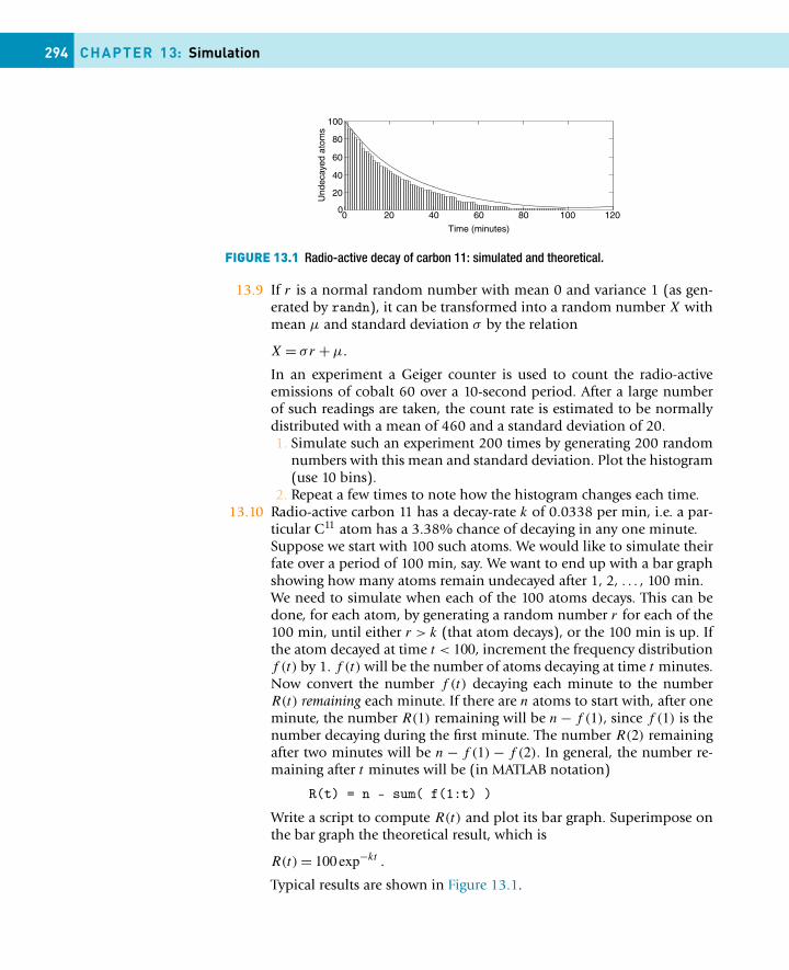
294 CHAPTER 13: Simulation
FIGURE 13.1 Radio-active decay of carbon 11: simulated and theoretical.
13.9 If r is a normal random number with mean 0 and variance 1 (as gen-erated by randn), it can be transformed into a random number X withmean μ and standard deviation σ by the relation
X = σr + μ.
In an experiment a Geiger counter is used to count the radio-activeemissions of cobalt 60 over a 10-second period. After a large numberof such readings are taken, the count rate is estimated to be normallydistributed with a mean of 460 and a standard deviation of 20.1. Simulate such an experiment 200 times by generating 200 random
numbers with this mean and standard deviation. Plot the histogram(use 10 bins).
2. Repeat a few times to note how the histogram changes each time.13.10 Radio-active carbon 11 has a decay-rate k of 0.0338 per min, i.e. a par-
ticular C11 atom has a 3.38% chance of decaying in any one minute.Suppose we start with 100 such atoms. We would like to simulate theirfate over a period of 100 min, say. We want to end up with a bar graphshowing how many atoms remain undecayed after 1, 2, . . . , 100 min.We need to simulate when each of the 100 atoms decays. This can bedone, for each atom, by generating a random number r for each of the100 min, until either r > k (that atom decays), or the 100 min is up. Ifthe atom decayed at time t < 100, increment the frequency distributionf (t) by 1. f (t) will be the number of atoms decaying at time t minutes.Now convert the number f (t) decaying each minute to the numberR(t) remaining each minute. If there are n atoms to start with, after oneminute, the number R(1) remaining will be n − f (1), since f (1) is thenumber decaying during the first minute. The number R(2) remainingafter two minutes will be n − f (1) − f (2). In general, the number re-maining after t minutes will be (in MATLAB notation)
R(t) = n - sum( f(1:t) )
Write a script to compute R(t) and plot its bar graph. Superimpose onthe bar graph the theoretical result, which is
R(t) = 100 exp−kt .
Typical results are shown in Figure 13.1.
CONTENTS
Equations............ 295Newton’s method .. 295Complex roots ......... 297The Bisectionmethod .................. 297fzero ..................... 299roots ..................... 299
Integration.......... 300The Trapezoidalrule ........................ 300Simpson’s rule ...... 301quad ....................... 302
Numericaldifferentiation .... 302diff ....................... 303
First-orderdifferentialequations ............ 304Euler’s method ...... 304Example: bacteriagrowth ................... 305Alternative subscriptnotation ................. 307A predictor-correctormethod .................. 307
CHAPTER 14
Introduction to Numerical Methods
THE OBJECTIVES OF THIS CHAPTER ARE TO INTRODUCENUMERICAL METHODS FOR:
� Solving equations.� Evaluating definite integrals.� Solving systems of ordinary differential equations.� Solving a parabolic partial differential equation.
A major scientific use of computers is in finding numerical solutions to math-ematical problems which have no analytical solutions (i.e., solutions whichmay be written down in terms of polynomials and standard mathematicalfunctions). In this chapter we look briefly at some areas where numerical meth-ods have been highly developed, e.g., solving non-linear equations, evaluatingintegrals, and solving differential equations.
14.1 EQUATIONS
In this section we consider how to solve equations in one unknown numeri-cally. The usual way of expressing the problem is to say that we want to solvethe equation f (x) = 0, i.e., we want to find its root (or roots). This processis also described as finding the zeros of f (x). There is no general method forfinding roots analytically for an arbitrary f (x).
14.1.1 Newton’s methodNewton’s method is perhaps the easiest numerical method to implement forsolving equations, and was introduced briefly in earlier chapters. It is an iter-ative method, meaning that it repeatedly attempts to improve an estimate ofthe root. If xk is an approximation to the root, we can relate it to the nextapproximation xk+1 using the right-angle triangle in Figure 14.1:
295Essential MATLAB for Engineers and Scientists. DOI:10.1016/B978-0-08-100877-5.00016-5Copyright © 2017 Daniel T. Valentine. Published by Elsevier Ltd. All rights reserved.
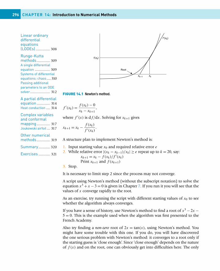
Linear ordinarydifferentialequations(LODEs) ............... 308
Runge-Kuttamethods .............. 309A single differentialequation ................ 309Systems of differentialequations: chaos .... 310Passing additionalparameters to an ODEsolver..................... 312
A partial differentialequation .............. 314Heat conduction .... 314
Complex variablesand conformalmapping .............. 317Joukowski airfoil ... 317
Other numericalmethods .............. 319
Summary ............ 320
Exercises ............ 321
296 CHAPTER 14: Introduction to Numerical Methods
FIGURE 14.1 Newton’s method.
f ′(xk) = f (xk) − 0
xk − xk+1,
where f ′(x) is df/dx. Solving for xk+1 gives
xk+1 = xk − f (xk)
f ′(xk).
A structure plan to implement Newton’s method is:
1. Input starting value x0 and required relative error e
2. While relative error |(xk − xk−1)/xk| ≥ e repeat up to k = 20, say:xk+1 = xk − f (xk)/f
′(xk)
Print xk+1 and f (xk+1)
3. Stop.
It is necessary to limit step 2 since the process may not converge.
A script using Newton’s method (without the subscript notation) to solve theequation x3 + x − 3 = 0 is given in Chapter 7. If you run it you will see that thevalues of x converge rapidly to the root.
As an exercise, try running the script with different starting values of x0 to seewhether the algorithm always converges.
If you have a sense of history, use Newton’s method to find a root of x3 − 2x −5 = 0. This is the example used when the algorithm was first presented to theFrench Academy.
Also try finding a non-zero root of 2x = tan(x), using Newton’s method. Youmight have some trouble with this one. If you do, you will have discoveredthe one serious problem with Newton’s method: it converges to a root only ifthe starting guess is ‘close enough’. Since ‘close enough’ depends on the natureof f (x) and on the root, one can obviously get into difficulties here. The only
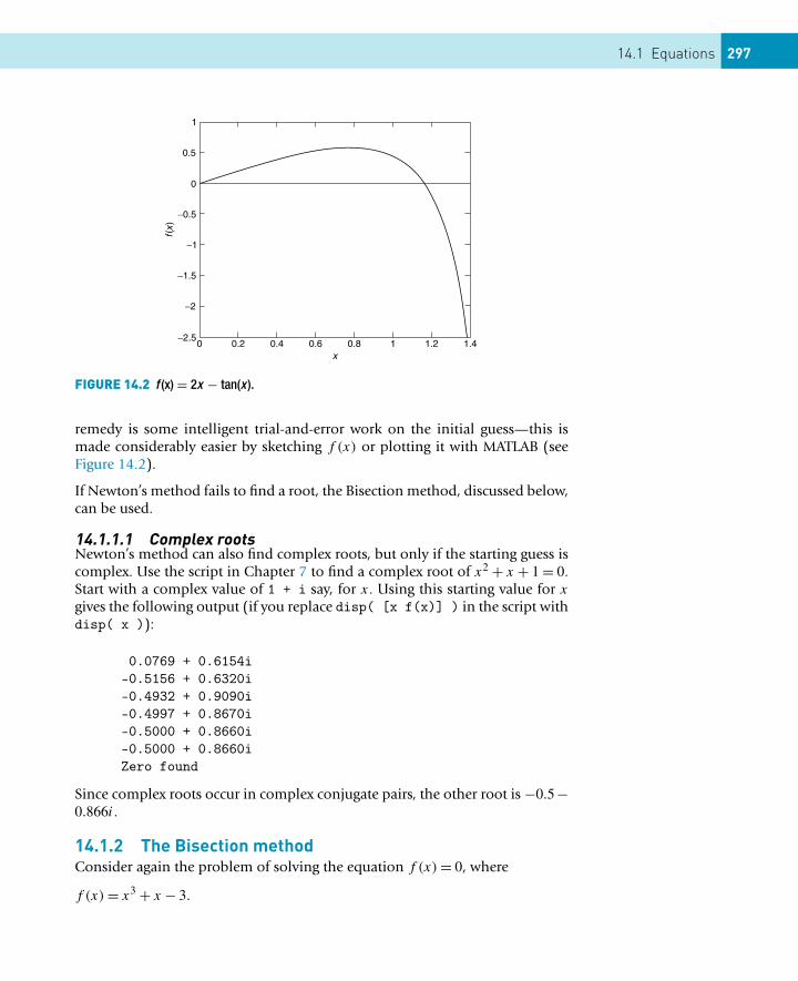
14.1 Equations 297
FIGURE 14.2 f (x) = 2x − tan(x ).
remedy is some intelligent trial-and-error work on the initial guess—this ismade considerably easier by sketching f (x) or plotting it with MATLAB (seeFigure 14.2).
If Newton’s method fails to find a root, the Bisection method, discussed below,can be used.
14.1.1.1 Complex rootsNewton’s method can also find complex roots, but only if the starting guess iscomplex. Use the script in Chapter 7 to find a complex root of x2 + x + 1 = 0.Start with a complex value of 1 + i say, for x. Using this starting value for x
gives the following output (if you replace disp( [x f(x)] ) in the script withdisp( x )):
0.0769 + 0.6154i-0.5156 + 0.6320i-0.4932 + 0.9090i-0.4997 + 0.8670i-0.5000 + 0.8660i-0.5000 + 0.8660iZero found
Since complex roots occur in complex conjugate pairs, the other root is −0.5 −0.866i.
14.1.2 The Bisection methodConsider again the problem of solving the equation f (x) = 0, where
f (x) = x3 + x − 3.
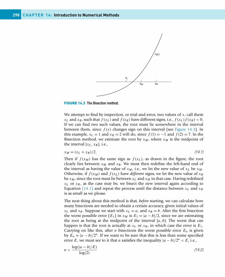
298 CHAPTER 14: Introduction to Numerical Methods
FIGURE 14.3 The Bisection method.
We attempt to find by inspection, or trial-and-error, two values of x, call themxL and xR , such that f (xL) and f (xR) have different signs, i.e., f (xL)f (xR) < 0.If we can find two such values, the root must lie somewhere in the intervalbetween them, since f (x) changes sign on this interval (see Figure 14.3). Inthis example, xL = 1 and xR = 2 will do, since f (1) = −1 and f (2) = 7. In theBisection method, we estimate the root by xM , where xM is the midpoint ofthe interval [xL, xR], i.e.,
xM = (xL + xR)/2. (14.1)
Then if f (xM) has the same sign as f (xL), as drawn in the figure, the rootclearly lies between xM and xR . We must then redefine the left-hand end ofthe interval as having the value of xM , i.e., we let the new value of xL be xM .Otherwise, if f (xM) and f (xL) have different signs, we let the new value of xR
be xM , since the root must lie between xL and xM in that case. Having redefinedxL or xR , as the case may be, we bisect the new interval again according toEquation (14.1) and repeat the process until the distance between xL and xR
is as small as we please.
The neat thing about this method is that, before starting, we can calculate howmany bisections are needed to obtain a certain accuracy, given initial values ofxL and xR . Suppose we start with xL = a, and xR = b. After the first bisectionthe worst possible error (E1) in xM is E1 = |a − b|/2, since we are estimatingthe root as being at the midpoint of the interval [a, b]. The worst that canhappen is that the root is actually at xL or xR , in which case the error is E1.Carrying on like this, after n bisections the worst possible error En is givenby En = |a − b|/2n. If we want to be sure that this is less than some specifiederror E, we must see to it that n satisfies the inequality |a − b|/2n < E, i.e.,
n >log(|a − b|/E)
log(2)(14.2)
14.1 Equations 299
Since n is the number of bisections, it must be an integer. The smallest integern that exceeds the right-hand side of Inequality (14.2) will do as the maximumnumber of bisections required to guarantee the given accuracy E.
The following scheme may be used to program the Bisection method. It willwork for any function f (x) that changes sign (in either direction) between thetwo values a and b, which must be found beforehand by the user.
1. Input a, b and E
2. Initialize xL and xR
3. Compute maximum bisections n from Inequality (14.2)4. Repeat n times:
Compute xM according to Equation (14.1)If f (xL)f (xM) > 0 then
Let xL = xM
otherwiseLet xR = xM
5. Display root xM
6. Stop.
We have assumed that the procedure will not find the root exactly; the chancesof this happening with real variables are infinitesimal.
The main advantage of the Bisection method is that it is guaranteed to finda root if you can find two starting values for xL and xR between which thefunction changes sign. You can also compute in advance the number of bisec-tions needed to attain a given accuracy. Compared to Newton’s method it isinefficient. Successive bisections do not necessarily move closer to the root, asusually happens with Newton’s method. In fact, it is interesting to compare thetwo methods on the same function to see how many more steps the Bisectionmethod requires than Newton’s method. For example, to solve the equationx3 + x − 3 = 0, the Bisection method takes 21 steps to reach the same accuracyas Newton’s in five steps.
14.1.3 fzeroThe MATLAB function fzero(@f, a) finds the zero nearest to the value a ofthe function f represented by the function f.m.
Use it to find a zero of x3 + x − 3.
fzero doesn’t appear to be able to find complex roots.
14.1.4 rootsThe MATLAB function M-file roots(c) finds all the roots (zeros) of the poly-nomial with coefficients in the vector c. See help for details.
Use it to find a zero of x3 + x − 3.
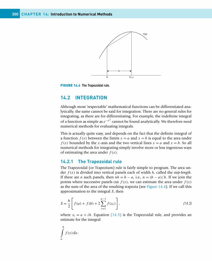
300 CHAPTER 14: Introduction to Numerical Methods
FIGURE 14.4 The Trapezoidal rule.
14.2 INTEGRATION
Although most ‘respectable’ mathematical functions can be differentiated ana-lytically, the same cannot be said for integration. There are no general rules forintegrating, as there are for differentiating. For example, the indefinite integralof a function as simple as e−x2
cannot be found analytically. We therefore neednumerical methods for evaluating integrals.
This is actually quite easy, and depends on the fact that the definite integral ofa function f (x) between the limits x = a and x = b is equal to the area underf (x) bounded by the x-axis and the two vertical lines x = a and x = b. So allnumerical methods for integrating simply involve more or less ingenious waysof estimating the area under f (x).
14.2.1 The Trapezoidal ruleThe Trapezoidal (or Trapezium) rule is fairly simple to program. The area un-der f (x) is divided into vertical panels each of width h, called the step-length.If there are n such panels, then nh = b − a, i.e., n = (b − a)/h. If we join thepoints where successive panels cut f (x), we can estimate the area under f (x)
as the sum of the area of the resulting trapezia (see Figure 14.4). If we call thisapproximation to the integral S, then
S = h
2
[f (a) + f (b) + 2
n−1∑i=1
f (xi)
], (14.3)
where xi = a + ih. Equation (14.3) is the Trapezoidal rule, and provides anestimate for the integral
b∫a
f (x)dx.
14.2 Integration 301
Here is a function to implement the Trapezoidal rule:
function y = trap( fn, a, b, h )n = (b-a)/h;x = a + [1:n-1]*h;y = sum(feval(fn, x));y = h/2*(feval(fn, a) + feval(fn, b) + 2*y);
Note:
1. Since the summation in the rule is implemented with a vectorized formularather than a for loop (to save time), the function to be integrated mustuse array operators where appropriate in its M-file implementation.
2. The user must choose h in such a way that the number of steps n will be aninteger—a check for this could be built in.
As an exercise, integrate f (x) = x3 between the limits 0 and 4 (remember towrite x.^3 in the function M-file). Call trap as follows:
s = trap(@f, 0, 4, h);
With h = 0.1, the estimate is 64.04, and with h = 0.01 it is 64.0004 (the exactintegral is 64). You will find that as h gets smaller, the estimate gets moreaccurate.
This example assumes that f (x) is a continuous function which may be eval-uated at any x. In practice, the function could be defined at discrete pointssupplied as results of an experiment. For example, the speed of an object v(t)
might be measured every so many seconds, and one might want to estimatethe distance traveled as the area under the speed-time graph. In this case, trapwould have to be changed by replacing fn with a vector of function values.This is left as an exercise for the curious. Alternatively, you can use the MAT-LAB function interp1 to interpolate the data. See help.
14.2.2 Simpson’s ruleSimpson’s rule is a method of numerical integration which is a good deal moreaccurate than the Trapezoidal rule, and should always be used before you tryanything fancier. It also divides the area under the function to be integrated,f (x), into vertical strips, but instead of joining the points f (xi) with straightlines, every set of three such successive points is fitted with a parabola. Toensure that there are always an even number of panels, the step-length h isusually chosen so that there are 2n panels, i.e., n = (b − a)/(2h).
Using the same notation as above, Simpson’s rule estimates the integral as
S = h
3
[f (a) + f (b) + 2
n−1∑i=1
f (x2i ) + 4n∑
i=1
f (x2i−1)
]. (14.4)
302 CHAPTER 14: Introduction to Numerical Methods
Coding this formula into a function M-file is left as an exercise.
If you try Simpson’s rule on f (x) = x3 between any limits, you will find rathersurprisingly, that it gives the same result as the exact mathematical solution.This is a nice extra benefit of the rule: it integrates cubic polynomials exactly(which can be proved).
14.2.3 quad
Not surprisingly, MATLAB has a function quad to carry out numerical integra-tion, or quadrature as it is also called. See help.
You may think there is no point in developing our own function files to handlethese numerical procedures when MATLAB has its own. If you have got this far,you should be curious enough to want to know how they work, rather thantreating them simply as ‘black boxes’.
14.3 NUMERICAL DIFFERENTIATION
The Newton quotient for a function f (x) is given by
f (x + h) − f (x)
h, (14.5)
where h is ‘small’. As h tends to zero, this quotient approaches the first deriva-tive, df/dx. The Newton quotient may therefore be used to estimate a deriva-tive numerically. It is a useful exercise to do this with a few functions forwhich you know the derivatives. This way you can see how small you canmake h before rounding errors cause problems. Such errors arise because ex-pression (14.5) involves subtracting two terms that eventually become equalwhen the limit of the computer’s accuracy is reached.
As an example, the following script uses the Newton quotient to estimate f ′(x)
for f (x) = x2 (which must be supplied as a function file f.m) at x = 2, forsmaller and smaller values of h (the exact answer is 4).
h = 1;x = 2;format short efor i = 1:20
nq = (f(x+h) - f(x))/h;disp( [h nq] )h = h / 10;
end
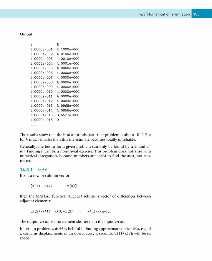
14.3 Numerical differentiation 303
Output:
1 51.0000e-001 4.1000e+0001.0000e-002 4.0100e+0001.0000e-003 4.0010e+0001.0000e-004 4.0001e+0001.0000e-005 4.0000e+0001.0000e-006 4.0000e+0001.0000e-007 4.0000e+0001.0000e-008 4.0000e+0001.0000e-009 4.0000e+0001.0000e-010 4.0000e+0001.0000e-011 4.0000e+0001.0000e-012 4.0004e+0001.0000e-013 3.9968e+0001.0000e-014 4.0856e+0001.0000e-015 3.5527e+0001.0000e-016 0...
The results show that the best h for this particular problem is about 10−8. Butfor h much smaller than this the estimate becomes totally unreliable.
Generally, the best h for a given problem can only be found by trial and er-ror. Finding it can be a non-trivial exercise. This problem does not arise withnumerical integration, because numbers are added to find the area, not sub-tracted.
14.3.1 diffIf x is a row or column vector
[x(1) x(2) ... x(n)]
then the MATLAB function diff(x) returns a vector of differences betweenadjacent elements:
[x(2)-x(1) x(3)-x(2) ... x(n)-x(n-1)]
The output vector is one element shorter than the input vector.
In certain problems, diff is helpful in finding approximate derivatives, e.g., ifx contains displacements of an object every h seconds, diff(x)/h will be itsspeed.
304 CHAPTER 14: Introduction to Numerical Methods
14.4 FIRST-ORDER DIFFERENTIAL EQUATIONS
The most interesting situations in real life that we may want to model, orrepresent quantitatively, are usually those in which the variables change intime (e.g., biological, electrical or mechanical systems). If the changes are con-tinuous, the system can often be represented with equations involving thederivatives of the dependent variables. Such equations are called differentialequations. The main aim of a lot of modeling is to be able to write down aset of differential equations (DEs) that describe the system being studied asaccurately as possible. Very few DEs can be solved analytically, so once again,numerical methods are required. We will consider the simplest method of nu-merical solution in this section: Euler’s method (Euler rhymes with ‘boiler’).We also consider briefly how to improve it.
14.4.1 Euler’s methodIn general we want to solve a first-order DE (strictly an ordinary—ODE) of theform
dy/dx = f (x, y), y(0) given.
Euler’s method for solving this DE numerically consists of replacing dy/dx
with its Newton quotient, so that the DE becomes
y(x + h) − y(x)
h= f (x, y).
After a slight rearrangement of terms, we get
y(x + h) = y(x) + hf (x, y). (14.6)
Solving a DE numerically is such an important and common problem in sci-ence and engineering that it is worth introducing some general notation atthis point. Suppose we want to integrate the DE over the interval x = a (a = 0usually) to x = b. We break this interval up into m steps of length h, so
m = (b − a)/h
(this is the same as the notation used in the update process of Chapter 10,except that dt used there has been replaced by the more general h here).
For consistency with MATLAB’s subscript notation, if we define yi as y(xi) (theEuler estimate at the beginning of step i), where xi = (i − 1)h, then yi+1 =y(x + h), at the end of step i. We can then replace Equation (14.6) by theiterative scheme
yi+1 = yi + hf (xi, yi), (14.7 )
where y1 = y(0). Recall from Chapter 10 that this notation enables us to gener-ate a vector y which we can then plot. Note also the striking similarity between
14.4 First-order differential equations 305
Equation (14.7) and the equation in Chapter 10 representing an update pro-cess. This similarity is no coincidence. Update processes are typically modeledby DEs, and Euler’s method provides an approximate solution for such DEs.
14.4.2 Example: bacteria growthSuppose a colony of 1000 bacteria is multiplying at the rate of r = 0.8 per hourper individual (i.e. an individual produces an average of 0.8 offspring everyhour). How many bacteria are there after 10 hours? Assuming that the colonygrows continuously and without restriction, we can model this growth withthe DE
dN/dt = rN, N(0) = 1000, (14.8)
where N(t) is the population size at time t . This process is called exponentialgrowth. Equation (14.8) may be solved analytically to give the well-known for-mula for exponential growth:
N(t) = N(0)ert .
To solve Equation (14.8) numerically, we apply Euler’s algorithm to it to get
Ni+1 = Ni + rhNi, (14.9)
where the initial value N1 = 1000.
It is very easy to program Euler’s method. The following script implementsEquation (14.9), taking h = 0.5. It also computes the exact solution for com-parison.
h = 0.5;r = 0.8;a = 0;b = 10;m = (b - a) / h;N = zeros(1, m+1);N(1) = 1000;t = a:h:b;
for i = 1:mN(i+1) = N(i) + r * h * N(i);
end
Nex = N(1) * exp(r * t);format bankdisp( [t’ N’ Nex’] )
plot(t, N ), xlabel( ’Hours’ ), ylabel( ’Bacteria’ )
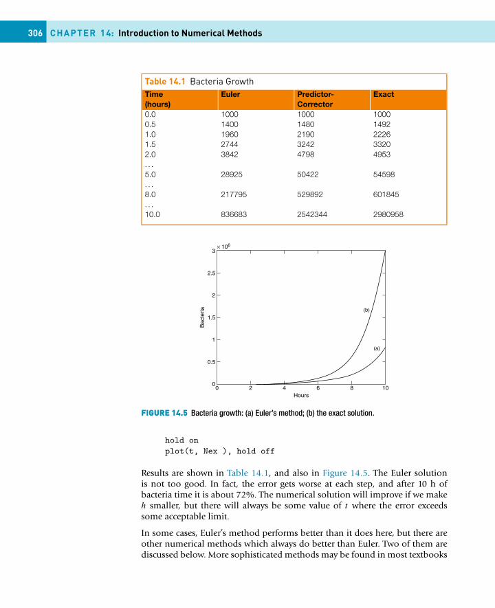
306 CHAPTER 14: Introduction to Numerical Methods
Table 14.1 Bacteria GrowthTime(hours)
Euler Predictor-Corrector
Exact
0.0 1000 1000 10000.5 1400 1480 14921.0 1960 2190 22261.5 2744 3242 33202.0 3842 4798 4953. . .
5.0 28925 50422 54598. . .
8.0 217795 529892 601845. . .
10.0 836683 2542344 2980958
FIGURE 14.5 Bacteria growth: (a) Euler’s method; (b) the exact solution.
hold onplot(t, Nex ), hold off
Results are shown in Table 14.1, and also in Figure 14.5. The Euler solutionis not too good. In fact, the error gets worse at each step, and after 10 h ofbacteria time it is about 72%. The numerical solution will improve if we makeh smaller, but there will always be some value of t where the error exceedssome acceptable limit.
In some cases, Euler’s method performs better than it does here, but there areother numerical methods which always do better than Euler. Two of them arediscussed below. More sophisticated methods may be found in most textbooks
14.4 First-order differential equations 307
on numerical analysis. However, Euler’s method may always be used as a firstapproximation as long as you realize that errors may arise.
14.4.3 Alternative subscript notationEquation (14.9) is an example of a finite difference scheme. The conventionalfinite difference notation is for the initial value to be represented by N0, i.e.with subscript i = 0. Ni is then the estimate at the end of step i. If you want theMATLAB subscripts in the Euler solution to be the same as the finite differencesubscripts, the initial value N0 must be represented by the MATLAB scalar N0,and you have to compute N(1) separately, before the for loop starts. You alsohave to display or plot the initial values separately since they will no longer beincluded in the MATLAB vectors t, N and Nex (which now have m instead ofm + 1 elements). Here is a complete script to generate the Euler solution usingfinite difference subscripts:
h = 0.5;r = 0.8;a = 0;b = 10;m = (b - a) / h;N = zeros(1, m); % one less element nowN0 = 1000;N(1) = N0 + r*h*N0; % no longer ’self-starting’
for i = 2:mN(i) = N(i-1) + r * h * N(i-1); %finite difference notation
end
t = a+h:h:b; % exclude initial time = aNex = N0 * exp(r * t);disp( [a N0 N0] ) % display initial values separatelydisp( [t’ N’ Nex’] )
plot(a, N0) % plot initial values separatelyhold onplot(t, N ), xlabel( ’Hours’ ), ylabel( ’Bacteria’ )plot(t, Nex ), hold off
14.4.4 A predictor-corrector methodOne improvement on the numerical solution of the first-order DE
dy/dx = f (x, y), y(0) given,
308 CHAPTER 14: Introduction to Numerical Methods
is as follows. The Euler approximation, which we are going to denote by anasterisk, is given by
y∗i+1 = yi + hf (xi, yi) (14.10)
But this formula favors the old value of y in computing f (xi, yi) on the right-hand side. Surely it would be better to say
y∗i+1 = yi + h[f (xi+1, y
∗i+1) + f (xi, yi)]/2, (14.11)
where xi+1 = xi +h, since this also involves the new value y∗i+1 in computing f
on the right-hand side? The problem of course is that y∗i+1 is as yet unknown,
so we can’t use it on the right-hand side of Equation (14.11). But we coulduse Euler to estimate (predict) y∗
i+1 from Equation (14.10) and then use Equa-tion (14.11) to correct the prediction by computing a better version of y∗
i+1,which we will call yi+1. So the full procedure is:
Repeat as many times as required:Use Euler to predict: y∗
i+1 = yi + hf (xi, yi)
Then correct y∗i+1 to: yi+1 = yi + h[f (xi+1, y
∗i+1) + f (xi, yi)]/2.
This is called a predictor-corrector method. The script above can easily beadapted to this problem. The relevant lines of code are:
for i = 1:m % m steps of length dtne(i+1) = ne(i) + r * h * ne(i);np = nc(i) + r * h * nc(i);nc(i+1) = nc(i) + r * h * (np + nc(i))/2;disp( [t(i+1) ne(i+1) nc(i+1) nex(i+1)] )
end;
ne stands for the ‘straight’ (uncorrected) Euler solution, np is the Euler predic-tor (since this is an intermediate result a vector is not needed for np), and ncis the corrector. The worst error is now only 15%. This is much better than theuncorrected Euler solution, although there is still room for improvement.
14.5 LINEAR ORDINARY DIFFERENTIAL EQUATIONS(LODES)
Linear ODEs with constant coefficients may be solved analytically in terms ofmatrix exponentials, which are represented in MATLAB by the function expm. Foran example see MATLAB Help: Mathematics: Matrices and Linear Algebra:Matrix Powers and Exponentials.
14.6 Runge-Kutta methods 309
14.6 RUNGE-KUTTA METHODS
There are a variety of algorithms, under the general name of Runge-Kutta,which can be used to integrate systems of ODEs. The formulae involved arerather complicated; they can be found in most books on numerical analysis.
However, as you may have guessed, MATLAB has plenty of ODE solvers, whichare discussed in MATLAB Help: Mathematics: Differential Equations. Amongthem are ode23 (second/third order) and ode45 (fourth/fifth order), which im-plement Runge-Kutta methods. (The order of a numerical method is the powerof h (i.e., dt) in the leading error term. Since h is generally very small, thehigher the power, the smaller the error.) We will demonstrate the use of ode23and ode45 here, first with a single first-order DE, and then with systems of suchequations.
14.6.1 A single differential equationHere’s how to use ode23 to solve the bacteria growth problem, Equa-tion (14.8):
dN/dt = rN, N(0) = 1000.
1. Start by writing a function file for the right-hand side of the DE to be solved.The function must have input variables t and N in this case (i.e., inde-pendent and dependent variables of the DE), in that order, e.g., create thefunction file f.m as follows:
function y = f(t, Nr)y = 0.8 * Nr;
2. Now enter the following statements in the Command Window:
a = 0;b = 10;n0 = 1000;[t, Nr] = ode23(@f, [a:0.5:b], n0);
3. Note the input arguments of ode23:@f: a handle for the function f, which contains the right-hand side of theDE;[a:0.5:b]: a vector (tspan) specifying the range of integration. If tspanhas two elements ([a b]) the solver returns the solution evaluated at ev-ery integration step (the solver chooses the integration steps and may varythem). This form would be suitable for plotting. However, if you want todisplay the solution at regular time intervals, as we want to here, use theform of tspan with three elements as above. The solution is then returnedevaluated at each time in tspan. The accuracy of the solution is not affectedby the form of tspan used.n0: the initial value of the solution N .
310 CHAPTER 14: Introduction to Numerical Methods
4. The output arguments are two vectors: the solutions Nr at times t. For 10 hode23 gives a value of 2961338 bacteria. From the exact solution in Ta-ble 14.1 we see that the error here is only 0.7%.
If the solutions you get from ode23 are not accurate enough, you can requestgreater accuracy with an additional optional argument. See help.
If you need still more accurate numerical solutions, you can use ode45 instead.It gives a final value for the bacteria of 2981290—an error of about 0.01%.
14.6.2 Systems of differential equations: chaosThe reason that weather prediction is so difficult and forecasts are so erratic isno longer thought to be the complexity of the system but the nature of the DEsmodeling it. These DEs belong to a class referred to as chaotic. Such equationswill produce wildly different results when their initial conditions are changedinfinitesimally. In other words, accurate weather prediction depends cruciallyon the accuracy of the measurements of the initial conditions.
Edward Lorenz, a research meteorologist, discovered this phenomenon in1961. Although his original equations are far too complex to consider here,the following much simpler system has the same essential chaotic features:
dx/dt = 10(y − x), (14.12)
dy/dt = −xz + 28x − y, (14.13)
dz/dt = xy − 8z/3. (14.14)
This system of DEs may be solved very easily with the MATLAB ODE solvers.The idea is to solve the DEs with certain initial conditions, plot the solution,then change the initial conditions very slightly, and superimpose the new so-lution over the old one to see how much it has changed.
We begin by solving the system with the initial conditions x(0) = −2,y(0) = −3.5 and z(0) = 21.
1. Write a function file lorenz.m to represent the right-hand sides of the sys-tem as follows:
function f = lorenz(t, x)f = zeros(3,1);f(1) = 10 * (x(2) - x(1));f(2) = -x(1) * x(3) + 28 * x(1) - x(2);f(3) = x(1) * x(2) - 8 * x(3) / 3;
The three elements of the MATLAB vector x, i.e., x(1), x(2) and x(3),represent the three dependent scalar variables x, y and z respectively. Theelements of the vector f represent the right-hand sides of the three DEs.When a vector is returned by such a DE function it must be a column vec-tor, hence the statement
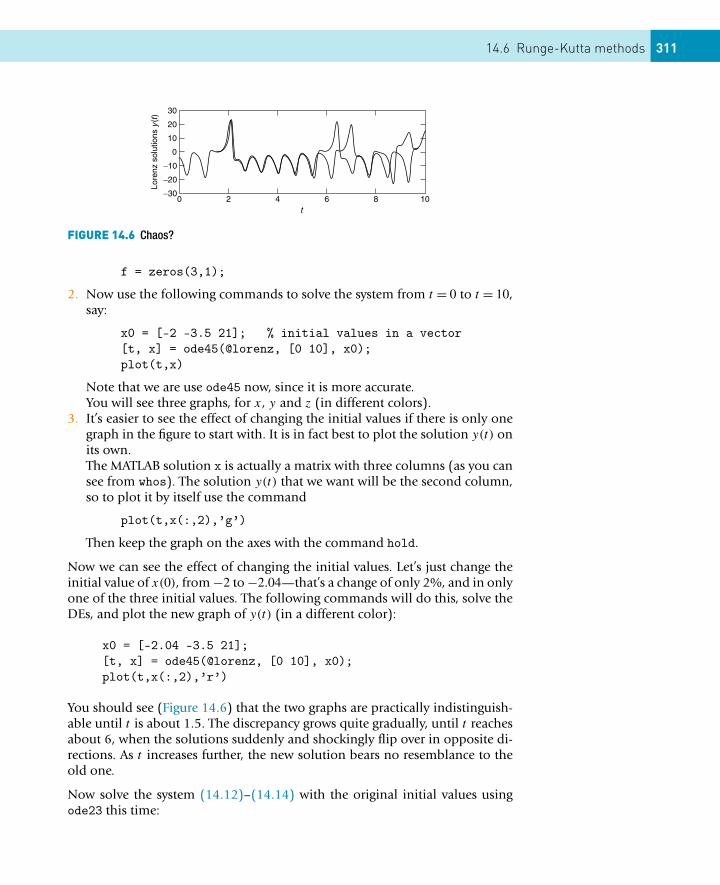
14.6 Runge-Kutta methods 311
FIGURE 14.6 Chaos?
f = zeros(3,1);
2. Now use the following commands to solve the system from t = 0 to t = 10,say:
x0 = [-2 -3.5 21]; % initial values in a vector[t, x] = ode45(@lorenz, [0 10], x0);plot(t,x)
Note that we are use ode45 now, since it is more accurate.You will see three graphs, for x, y and z (in different colors).
3. It’s easier to see the effect of changing the initial values if there is only onegraph in the figure to start with. It is in fact best to plot the solution y(t) onits own.The MATLAB solution x is actually a matrix with three columns (as you cansee from whos). The solution y(t) that we want will be the second column,so to plot it by itself use the command
plot(t,x(:,2),’g’)
Then keep the graph on the axes with the command hold.
Now we can see the effect of changing the initial values. Let’s just change theinitial value of x(0), from −2 to −2.04—that’s a change of only 2%, and in onlyone of the three initial values. The following commands will do this, solve theDEs, and plot the new graph of y(t) (in a different color):
x0 = [-2.04 -3.5 21];[t, x] = ode45(@lorenz, [0 10], x0);plot(t,x(:,2),’r’)
You should see (Figure 14.6) that the two graphs are practically indistinguish-able until t is about 1.5. The discrepancy grows quite gradually, until t reachesabout 6, when the solutions suddenly and shockingly flip over in opposite di-rections. As t increases further, the new solution bears no resemblance to theold one.
Now solve the system (14.12)–(14.14) with the original initial values usingode23 this time:
312 CHAPTER 14: Introduction to Numerical Methods
x0 = [-2 -3.5 21];[t,x] = ode23(@lorenz, [0 10], x0);
Plot the graph of y(t) only—x(:,2)—and then superimpose the ode45 solu-tion with the same initial values (in a different color).
A strange thing happens—the solutions begin to deviate wildly for t > 1.5!The initial conditions are the same—the only difference is the order of theRunge-Kutta method.
Finally solve the system with ode23s and superimpose the solution. (The sstands for ‘stiff’. For a stiff DE, solutions can change on a time scale that is veryshort compared to the interval of integration.) The ode45 and ode23s solutionsonly start to diverge at t > 5.
The explanation is that ode23, ode23s and ode45 all have numerical inaccura-cies (if one could compare them with the exact solution—which incidentallycan’t be found). However, the numerical inaccuracies are different in the threecases. This difference has the same effect as starting the numerical solutionwith very slightly different initial values.
How do we ever know when we have the ‘right’ numerical solution? Well, wedon’t—the best we can do is increase the accuracy of the numerical methoduntil no further wild changes occur over the interval of interest. So in our ex-ample we can only be pretty sure of the solution for t < 5 (using ode23s orode45). If that’s not good enough, you have to find a more accurate DE solver.
So beware: ‘chaotic’ DEs are very tricky to solve!
Incidentally, if you want to see the famous ‘butterfly’ picture of chaos, just plotx against z as time increases (the resulting graph is called a phase plane plot).The following command will do the trick:
plot(x(:,1), x(:,3))
What you will see is a static 2-D projection of the trajectory, i.e., the solutiondeveloping in time. Demos in the MATLAB Launch Pad include an examplewhich enables you to see the trajectory evolving dynamically in 3-D (Demos:Graphics: Lorenz attractor animation).
14.6.3 Passing additional parameters to an ODE solverIn the above examples of the MATLAB ODE solvers the coefficients in the right-hand sides of the DEs (e.g., the value 28 in Equation (14.13)) have all beenconstants. In a real modeling situation, you will most likely want to changesuch coefficients frequently. To avoid having to edit the function files each timeyou want to change a coefficient, you can pass the coefficients as additional
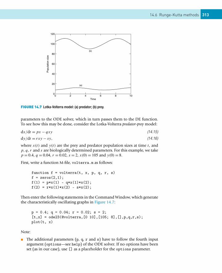
14.6 Runge-Kutta methods 313
FIGURE 14.7 Lotka-Volterra model: (a) predator; (b) prey.
parameters to the ODE solver, which in turn passes them to the DE function.To see how this may be done, consider the Lotka-Volterra predator-prey model:
dx/dt = px − qxy (14.15)
dy/dt = rxy − sy, (14.16)
where x(t) and y(t) are the prey and predator population sizes at time t , andp, q , r and s are biologically determined parameters. For this example, we takep = 0.4, q = 0.04, r = 0.02, s = 2, x(0) = 105 and y(0) = 8.
First, write a function M-file, volterra.m as follows:
function f = volterra(t, x, p, q, r, s)f = zeros(2,1);f(1) = p*x(1) - q*x(1)*x(2);f(2) = r*x(1)*x(2) - s*x(2);
Then enter the following statements in the Command Window, which generatethe characteristically oscillating graphs in Figure 14.7:
p = 0.4; q = 0.04; r = 0.02; s = 2;[t,x] = ode23(@volterra,[0 10],[105; 8],[],p,q,r,s);plot(t, x)
Note:
� The additional parameters (p, q, r and s) have to follow the fourth inputargument (options—see help) of the ODE solver. If no options have beenset (as in our case), use [] as a placeholder for the options parameter.
314 CHAPTER 14: Introduction to Numerical Methods
You can now change the coefficients from the Command Window and get anew solution, without editing the function file.
14.7 A PARTIAL DIFFERENTIAL EQUATION
The numerical solution of partial differential equations (PDEs) is a vast sub-ject, which is beyond the scope of this book. However, a class of PDEs calledparabolic often lead to solutions in terms of sparse matrices, which were men-tioned briefly in Chapter 6. One such example is considered in this section.
14.7.1 Heat conductionThe conduction of heat along a thin uniform rod may be modeled by the par-tial differential equation
∂u
∂t= ∂2u
∂x2, (14.17 )
where u(x, t) is the temperature distribution a distance x from one end of therod at time t , and assuming that no heat is lost from the rod along its length.
Half the battle in solving PDEs is mastering the notation. We set up a rectan-gular grid, with step-lengths of h and k in the x and t directions respectively.A general point on the grid has co-ordinates xi = ih, yj = jk. A concise nota-tion for u(x, t) at xi , yj is then simply ui,j .
Truncated Taylor series may then be used to approximate the PDE by a finite dif-ference scheme. The left-hand side of Equation (14.17) is usually approximatedby a forward difference:
∂u
∂t= ui,j+1 − ui,j
k
One way of approximating the right-hand side of Equation (14.17) is by thescheme
∂2u
∂x2= ui+1,j − 2ui,j + ui−1,j
h2. (14.18)
This leads to a scheme, which although easy to compute, is only conditionallystable.
If however we replace the right-hand side of the scheme in Equation (14.18)by the mean of the finite difference approximation on the j th and (j + 1)thtime rows, we get (after a certain amount of algebra!) the following scheme forEquation (14.17):
−rui−1,j+1 + (2 + 2r)ui,j+1 − rui+1,j+1 = rui−1,j + (2 − 2r)ui,j + rui+1,j ,
(14.19)
14.7 A partial differential equation 315
where r = k/h2. This is known as the Crank-Nicolson implicit method, since itinvolves the solution of a system of simultaneous equations, as we shall see.
To illustrate the method numerically, let’s suppose that the rod has a lengthof 1 unit, and that its ends are in contact with blocks of ice, i.e., the boundaryconditions are
u(0, t) = u(1, t) = 0. (14.20)
Suppose also that the initial temperature (initial condition) is
u(x,0) ={
2x, 0 ≤ x ≤ 1/2,
2(1 − x), 1/2 ≤ x ≤ 1(14.21)
(this situation could come about by heating the center of the rod for a longtime, with the ends kept in contact with the ice, removing the heat source attime t = 0). This particular problem has symmetry about the line x = 1/2; weexploit this now in finding the solution.
If we take h = 0.1 and k = 0.01, we will have r = 1, and Equation (14.19)becomes
−ui−1,j+1 + 4ui,j+1 − ui+1,j+1 = ui−1,j + ui+1,j . (14.22)
Putting j = 0 in Equation (14.22) generates the following set of equations forthe unknowns ui,1 (i.e., after one time step k) up to the midpoint of the rod,which is represented by i = 5, i.e., x = ih = 0.5. The subscript j = 1 has beendropped for clarity:
0 + 4u1 − u2 = 0 + 0.4
−u1 + 4u2 − u3 = 0.2 + 0.6
−u2 + 4u3 − u4 = 0.4 + 0.8
−u3 + 4u4 − u5 = 0.6 + 1.0
−u4 + 4u5 − u6 = 0.8 + 0.8.
Symmetry then allows us to replace u6 in the last equation by u4. These equa-tions can be written in matrix form as⎡⎢⎢⎢⎢⎣
4 −1 0 0 0−1 4 −1 0 0
0 −1 4 −1 00 0 −1 4 −10 0 0 −2 4
⎤⎥⎥⎥⎥⎦
⎡⎢⎢⎢⎢⎣
u1u2u3u4u5
⎤⎥⎥⎥⎥⎦ =
⎡⎢⎢⎢⎢⎣
0.40.81.21.61.6
⎤⎥⎥⎥⎥⎦ . (14.23)
The matrix (A) on the left of Equations (14.23) is known as a tridiagonal matrix.Having solved for the ui,1 we can then put j = 1 in Equation (14.22) andproceed to solve for the ui,2, and so on. The system (14.23) can of course besolved directly in MATLAB with the left division operator. In the script below,the general form of Equations (14.23) is taken as
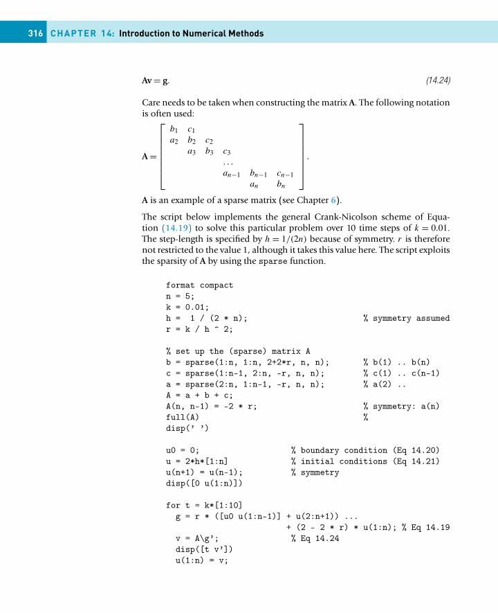
316 CHAPTER 14: Introduction to Numerical Methods
Av = g. (14.24)
Care needs to be taken when constructing the matrix A. The following notationis often used:
A =
⎡⎢⎢⎢⎢⎢⎢⎣
b1 c1a2 b2 c2
a3 b3 c3. . .
an−1 bn−1 cn−1an bn
⎤⎥⎥⎥⎥⎥⎥⎦
.
A is an example of a sparse matrix (see Chapter 6).
The script below implements the general Crank-Nicolson scheme of Equa-tion (14.19) to solve this particular problem over 10 time steps of k = 0.01.The step-length is specified by h = 1/(2n) because of symmetry. r is thereforenot restricted to the value 1, although it takes this value here. The script exploitsthe sparsity of A by using the sparse function.
format compactn = 5;k = 0.01;h = 1 / (2 * n); % symmetry assumedr = k / h ^ 2;
% set up the (sparse) matrix Ab = sparse(1:n, 1:n, 2+2*r, n, n); % b(1) .. b(n)c = sparse(1:n-1, 2:n, -r, n, n); % c(1) .. c(n-1)a = sparse(2:n, 1:n-1, -r, n, n); % a(2) ..A = a + b + c;A(n, n-1) = -2 * r; % symmetry: a(n)full(A) %disp(’ ’)
u0 = 0; % boundary condition (Eq 14.20)u = 2*h*[1:n] % initial conditions (Eq 14.21)u(n+1) = u(n-1); % symmetrydisp([0 u(1:n)])
for t = k*[1:10]g = r * ([u0 u(1:n-1)] + u(2:n+1)) ...
+ (2 - 2 * r) * u(1:n); % Eq 14.19v = A\g’; % Eq 14.24disp([t v’])u(1:n) = v;
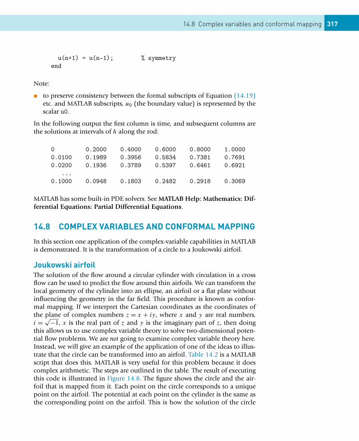
14.8 Complex variables and conformal mapping 317
u(n+1) = u(n-1); % symmetryend
Note:
� to preserve consistency between the formal subscripts of Equation (14.19)etc. and MATLAB subscripts, u0 (the boundary value) is represented by thescalar u0.
In the following output the first column is time, and subsequent columns arethe solutions at intervals of h along the rod:
0 0.2000 0.4000 0.6000 0.8000 1.00000.0100 0.1989 0.3956 0.5834 0.7381 0.76910.0200 0.1936 0.3789 0.5397 0.6461 0.6921
...0.1000 0.0948 0.1803 0.2482 0.2918 0.3069
MATLAB has some built-in PDE solvers. See MATLAB Help: Mathematics: Dif-ferential Equations: Partial Differential Equations.
14.8 COMPLEX VARIABLES AND CONFORMAL MAPPING
In this section one application of the complex-variable capabilities in MATLABis demonstrated. It is the transformation of a circle to a Joukowski airfoil.
Joukowski airfoilThe solution of the flow around a circular cylinder with circulation in a crossflow can be used to predict the flow around thin airfoils. We can transform thelocal geometry of the cylinder into an ellipse, an airfoil or a flat plate withoutinfluencing the geometry in the far field. This procedure is known as confor-mal mapping. If we interpret the Cartesian coordinates as the coordinates ofthe plane of complex numbers z = x + iy, where x and y are real numbers,i = √−1, x is the real part of z and y is the imaginary part of z, then doingthis allows us to use complex variable theory to solve two-dimensional poten-tial flow problems. We are not going to examine complex variable theory here.Instead, we will give an example of the application of one of the ideas to illus-trate that the circle can be transformed into an airfoil. Table 14.2 is a MATLABscript that does this. MATLAB is very useful for this problem because it doescomplex arithmetic. The steps are outlined in the table. The result of executingthis code is illustrated in Figure 14.8. The figure shows the circle and the air-foil that is mapped from it. Each point on the circle corresponds to a uniquepoint on the airfoil. The potential at each point on the cylinder is the same asthe corresponding point on the airfoil. This is how the solution of the circle
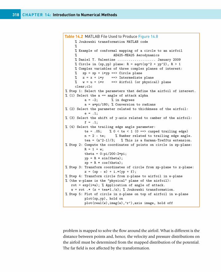
318 CHAPTER 14: Introduction to Numerical Methods
Table 14.2 MATLAB File Used to Produce Figure 14.8% Joukowski transformation MATLAB code%% Example of conformal mapping of a circle to an airfoil% AE425-ME425 Aerodynamics% Daniel T. Valentine .................... January 2009% Circle in (xp,yp) plane: R = sqrt(xp^2 + yp^2), R > 1% Complex variables of three complex planes of interest:% zp = xp + i*yp ==> Circle plane% z = x + i*y ==> Intermediate plane% w = u + i*v ==> Airfoil (or physical) planeclear;clc
% Step 1: Select the parameters that define the airfoil of interest.% (1) Select the a == angle of attack alpha
a = -2; % in degreesa = a*pi/180; % Conversion to radians
% (2) Select the parameter related to thichkness of the airfoil:e = .1;
% (3) Select the shift of y-axis related to camber of the airfoil:f = .1;
% (4) Select the trailing edge angle parameter:te = .05; % 0 < te < 1 (0 ==> cusped trailing edge)n = 2 - te; % Number related to trailing edge angle.tea = (n^2-1)/3; % This is a Karman-Trefftz extension.
% Step 2: Compute the coordinates of points on circle in zp-plane:R = 1 + e;theta = 0:pi/200:2*pi;yp = R * sin(theta);xp = R * cos(theta);
% Step 3: Transform coordinates of circle from zp-plane to z-plane:z = (xp - e) + i.*(yp + f);
% Step 4: Transform circle from z-plane to airfoil in w-plane% (the w-plane is the "physical" plane of the airfoil):
rot = exp(i*a); % Application of angle of attack.w = rot .* (z + tea*1./z); % Joukowski transformation.
% Step 5: Plot of circle in z-plane on top of airfoil in w-planeplot(xp,yp), hold onplot(real(w),imag(w),’r’),axis image, hold off
problem is mapped to solve the flow around the airfoil. What is different is thedistance between points and, hence, the velocity and pressure distributions onthe airfoil must be determined from the mapped distribution of the potential.The far field is not affected by the transformation.
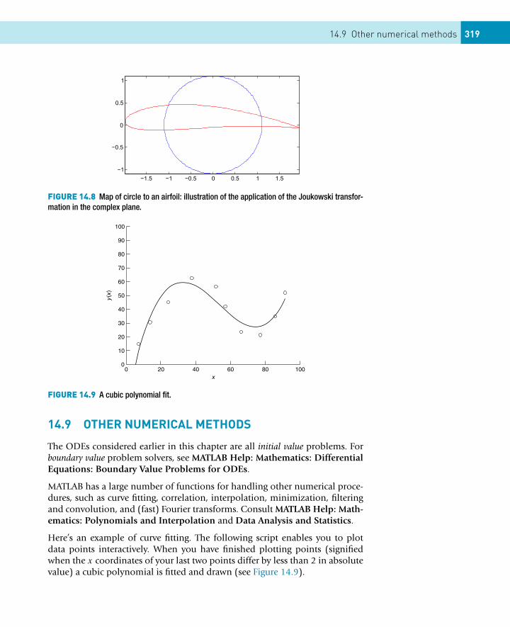
14.9 Other numerical methods 319
FIGURE 14.8 Map of circle to an airfoil: illustration of the application of the Joukowski transfor-mation in the complex plane.
FIGURE 14.9 A cubic polynomial fit.
14.9 OTHER NUMERICAL METHODS
The ODEs considered earlier in this chapter are all initial value problems. Forboundary value problem solvers, see MATLAB Help: Mathematics: DifferentialEquations: Boundary Value Problems for ODEs.
MATLAB has a large number of functions for handling other numerical proce-dures, such as curve fitting, correlation, interpolation, minimization, filteringand convolution, and (fast) Fourier transforms. Consult MATLAB Help: Math-ematics: Polynomials and Interpolation and Data Analysis and Statistics.
Here’s an example of curve fitting. The following script enables you to plotdata points interactively. When you have finished plotting points (signifiedwhen the x coordinates of your last two points differ by less than 2 in absolutevalue) a cubic polynomial is fitted and drawn (see Figure 14.9).

320 CHAPTER 14: Introduction to Numerical Methods
% Interactive script to fit a cubic to data points
clfhold onaxis([0 100 0 100]);
diff = 10;xold = 68;i = 0;xp = zeros(1); % data pointsyp = zeros(1);
while diff > 2[a b] = ginput(1);diff = abs(a - xold);if diff > 2
i = i + 1;xp(i) = a;yp(i) = b;xold = a;plot(a, b, ’ok’)
endend
p = polyfit(xp, yp, 3 );x = 0:0.1:xp(length(xp));y= p(1)*x.^3 + p(2)*x.^2 + p(3)*x + p(4);plot(x,y), title( ’cubic polynomial fit’), ...
ylabel(’y(x)’), xlabel(’x’)hold off
Polynomial fitting may also be done interactively in a figure window, withTools -> Basic Fitting.
SUMMARY� A numerical method is an approximate computer method for solving a
mathematical problem which often has no analytical solution.� A numerical method is subject to two distinct types of error: rounding error
in the computer solution, and truncation error, where an infinite mathemat-ical process, like taking a limit, is approximated by a finite process.
� MATLAB has a large number of useful functions for handling numericalmethods.
14.9 Exercises 321
EXERCISES14.1 Use Newton’s method in a script to solve the following (you may have to
experiment a bit with the starting values). Check all your answers withfzero. Check the answers involving polynomial equations with roots.Hint: use fplot to get an idea of where the roots are, e.g.,
fplot(’x^3-8*x^2+17*x-10’, [0 3])
The Zoom feature also helps. In the figure window select the Zoom Inbutton (magnifying glass) and click on the part of the graph you wantto magnify.(a) x4 − x = 10 (two real roots and two complex roots)(b) e−x = sinx (infinitely many roots)(c) x3 − 8x2 + 17x − 10 = 0 (three real roots)(d) logx = cosx
(e) x4 − 5x3 − 12x2 + 76x − 79 = 0 (four real roots)14.2 Use the Bisection method to find the square root of 2, taking 1 and 2 as
initial values of xL and xR . Continue bisecting until the maximum erroris less than 0.05 (use Inequality (14.2) of Section 14.1 to determine howmany bisections are needed).
14.3 Use the Trapezoidal rule to evaluate∫ 4
0 x2dx, using a step-length ofh = 1.
14.4 A human population of 1000 at time t = 0 grows at a rate given by
dN/dt = aN,
where a = 0.025 per person per year. Use Euler’s method to project thepopulation over the next 30 years, working in steps of (a) h = 2 years,(b) h = 1 year and (c) h = 0.5 years. Compare your answers with theexact mathematical solution.
14.5 Write a function file euler.m which starts with the line
function [t, n] = euler(a, b, dt)
and which uses Euler’s method to solve the bacteria growth DE (14.8).Use it in a script to compare the Euler solutions for dt = 0.5 and 0.05with the exact solution. Try to get your output looking like this:
time dt = 0.5 dt = 0.05 exact
0 1000.00 1000.00 1000.000.50 1400.00 1480.24 1491.821.00 1960.00 2191.12 2225.54...
5.00 28925.47 50504.95 54598.15
14.6 The basic equation for modeling radio-active decay is
322 CHAPTER 14: Introduction to Numerical Methods
dx/dt = −rx,
where x is the amount of the radio-active substance at time t , and r isthe decay rate.Some radio-active substances decay into other radio-active substances,which in turn also decay. For example, Strontium 92 (r1 = 0.256 per hr)decays into Yttrium 92 (r2 = 0.127 per hr), which in turn decays intoZirconium. Write down a pair of differential equations for Strontiumand Yttrium to describe what is happening.Starting at t = 0 with 5 × 1026 atoms of Strontium 92 and none of Yt-trium, use the Runge-Kutta method (ode23) to solve the equations up tot = 8 hr in steps of 1/3 hr. Also use Euler’s method for the same problem,and compare your results.
14.7 The springbok (a species of small buck, not rugby players!) populationx(t) in the Kruger National Park in South Africa may be modeled by theequation
dx/dt = (r − bx sinat)x,
where r , b, and a are constants. Write a program which reads values forr , b, and a, and initial values for x and t , and which uses Euler’s methodto compute the impala population at monthly intervals over a period oftwo years.
14.8 The luminous efficiency (ratio of the energy in the visible spectrum tothe total energy) of a black body radiator may be expressed as a percent-age by the formula
E = 64.77T −4
7×10⁻⁵∫4×10⁻⁵
x−5(e1.432/T x − 1)−1dx,
where T is the absolute temperature in degrees Kelvin, x is the wave-length in cm, and the range of integration is over the visible spectrum.Write a general function simp(fn, a, b, h) to implement Simpson’srule as given in Equation (14.4).Taking T = 3500 K, use simp to compute E, firstly with 10 intervals(n = 5), and then with 20 intervals (n = 10), and compare your results.(Answers: 14.512725% for n = 5; 14.512667% for n = 10)
14.9 Van der Pol’s equation is a second-order non-linear differential equationwhich may be expressed as two first-order equations as follows:
dx1/dt = x2
dx2/dt = ε(1 − x21)x2 − b2x1.
The solution of this system has a stable limit cycle, which means thatif you plot the phase trajectory of the solution (the plot of x1 againstx2) starting at any point in the positive x1-x2 plane, it always moves
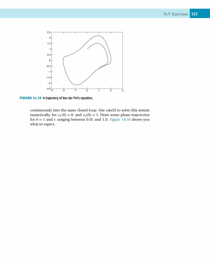
14.9 Exercises 323
FIGURE 14.10 A trajectory of Van der Pol’s equation.
continuously into the same closed loop. Use ode23 to solve this systemnumerically, for x1(0) = 0, and x2(0) = 1. Draw some phase trajectoriesfor b = 1 and ε ranging between 0.01 and 1.0. Figure 14.10 shows youwhat to expect.
CONTENTS
Harmonicanalysis ............... 326
Fast FourierTransform (FFT) 331
CHAPTER 15
Signal Processing
THE OBJECTIVE OF THIS CHAPTER IS TO INTRODUCESIGNAL PROCESSING. YOU WILL LEARN ABOUT TWOMETHODS, OF MANY, TO EXAMINE LARGE DATA SETS. THEYARE:
� Harmonic analysis.� Fast Fourier Transform analysis.
In this chapter we apply MATLAB to examine periodic data sets. Harmonicanalysis is introduced in the next section to examine periodic data sets. In thesubsequent section the fast Fourier transform (FFT) method is applied to exam-ine the temporal-evolution of measured or computed data. These proceduresare important methods in the field of signal processing.
A signal is a sequence of data that is measured by experimental methods orcomputed by computational methods. For example, the data f (x) is measuredat relatively small intervals of a particular variable x, e.g., x could be time ora space dimension. If the signal is periodic in a range of x, e.g., −π to π ,harmonic analysis is a useful and quite practical technique. The FFT method isa related method. Both methods are associated with the fitting of data with aFourier series. In addition, both methods are widely used in engineering, e.g.,in naval architecture, acoustics (or noise) and vibration engineering, electricalengineering, ocean engineering, etc.
The theory of Fourier series is an important topic in mathematics for physicistsand engineers. A reasonably thorough discussion of this topic can be found inMathematics of Physics and Modern Engineering, Second Edition, by I.S. Sokol-nikoff and R.M. Redheffer, a book published by McGraw-Hill (1966). Becauseof the importance of this topic, it should not be surprising that there are manyother books that describe the theory behind the method and the practicalapplications of the method. In this introductory section we give the results
325Essential MATLAB for Engineers and Scientists. DOI:10.1016/B978-0-08-100877-5.00017-7Copyright © 2017 Daniel T. Valentine. Published by Elsevier Ltd. All rights reserved.
326 CHAPTER 15: Signal Processing
associated with applying the Fourier series method that are needed to examinesignals.
Let us suppose f (x) is given by the trigonometric series
f (x) = 1
2ao +
∞∑n=1
(an cosnx + bn sinnx) (15.1)
where −π ≤ x ≤ π and, hence,
an = 1
π
π∫−π
f (x) cosnx dx (15.2)
for n = 0, 1, 2, . . ., and
bn = 1
π
π∫−π
f (x) sinnx dx (15.3)
for n = 1, 2, 3, . . .. This assumes that the function f (x) is periodic, i.e., f (x) =f (x + 2π).
If we are given a data set f (x) and it is assumed to be periodic in the interval−π ≤ x ≤ π , we can compute the coefficients an and bn by applying the aboveformulas. With this approach we say that we expanded f (x) in or say that f (x)
has the Fourier series
f (x) ∼ 1
2Ao +
N∑n=1
(An cosnx + Bn sinnx) (15.4)
where N is a positive integer greater than or equal to 1. It is the number ofterms to be evaluated to construct a Fourier series (or Fourier expansion) off (x). If N → ∞ and f (x) is continuous and periodic, the last equation isessentially the trigonometric expansion of f (x) and the result is exact. An im-portant advantage of this series is that it can represent discontinuous functionsas well. Of course, in this case or in cases where the trigonometric representa-tion is not exact, it is a best fit representation of f (x) in terms of the assumedperiodic function, Equation (15.4).
15.1 HARMONIC ANALYSIS
Let us examine the data illustrated in Figure 15.1 by fitting a trigonometricseries through the data. This sample set of “observed” data was generated byusing the following formula:
f = .6 − cosx − .5 cos 2x + .4 cos 3x + sinx + error, (15.5)
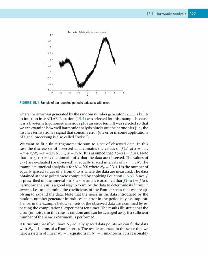
15.1 Harmonic analysis 327
FIGURE 15.1 Sample of ten repeated periodic data sets with error.
where the error was generated by the random number generator randn, a built-in function in MATLAB. Equation (15.5) was selected for this example becauseit is a five-term trigonometric serious plus an error term. It was selected so thatwe can examine how well harmonic analysis plucks out the harmonics (i.e., thefirst five terms) from a signal that contains error (the error in some applicationsof signal processing is also called “noise”).
We want to fit a finite trigonometric sum to a set of observed data. In thiscase the discrete set of observed data contains the values of f (x) at x = −π ,−π + π/N , −π + 2π/N , . . ., π − π/N . It is assumed that f (−π) = f (π). Notethat −π ≤ x < π is the domain of x that the data are observed. The values off (x) are evaluated (or observed) at equally spaced intervals of dx = π/N . Theexample numerical analysis is for N = 200 where Np = 2N +1 is the number ofequally spaced values of f from 0 to π where the data are measured. The dataobtained at these points were computed by applying Equation (15.5). Since f
is prescribed on the interval −π ≤ x ≤ π and it is assumed that f (−π) = f (π),harmonic analysis is a good way to examine the data to determine its harmoniccontent, i.e., to determine the coefficients of the Fourier series that we are ap-plying to expand the data. Note that the noise in the data introduced by therandom number generator introduces an error in the periodicity assumption.Hence, in the example below ten sets of the observed data are examined by re-peating the computational experiment ten times. The results illustrate that theerror (or noise), in this case, is random and can be averaged away if a sufficientnumber of the same experiment is performed.
It turns out that if you have Np equally spaced data points we can fit the datawith Np − 1 terms of a Fourier series. The results are exact in the sense that wehave a system of linear Np − 1 equations in Np − 1 unknowns. It is reasonably
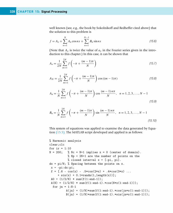
328 CHAPTER 15: Signal Processing
well known (see, e.g., the book by Sokolnikoff and Redheffer cited above) thatthe solution to this problem is
f = Ao +N∑
n=1
An cosnx +N−1∑n=1
Bn sinnx (15.6)
(Note that Ao is twice the value of ao in the Fourier series given in the intro-duction to this chapter.) In this case, it can be shown that
Ao = 1
2N
2N∑m=1
f
(−π + (m − 1)π
N
)(15.7 )
AN = 1
2N
2N∑m=1
f
(−π + (m − 1)π
N
)cos ((m − 1)π) (15.8)
An = 1
N
2N∑m=1
f
(−π + (m − 1)π
N
)cos
(m − 1) nπ
N, n = 1,2,3, . . . ,N − 1
(15.9)
Bn = 1
N
2N∑m=1
f
(−π + (m − 1)π
N
)sin
(m − 1) nπ
N, n = 1,2,3, . . . ,N − 1
(15.10)
This system of equations was applied to examine the data generated by Equa-tion (15.5). The MATLAB script developed and applied is as follows:
% Harmonic analysisclear;clcfor ir = 1:10N = 200; % Nc = N+1 implies x = 0 (center of domain).
% Np = 2N+1 are the number of points on the% closed interval x = [-pi, pi].
dx = pi/N; % Spacing between the points on x.x = -pi:dx:pi;f = [.6 - cos(x) - .5*cos(2*x) + .4*cos(3*x) ...
+ sin(x) + 0.1*randn(1,length(x))];A0 = (1/2/N) * sum(f(1:end-1));A(N) = (1/2/N) * sum(f(1:end-1).*cos(N*x(1:end-1)));for jn = 1:N-1
A(jn) = (1/N)*sum(f(1:end-1).*cos(jn*x(1:end-1)));B(jn) = (1/N)*sum(f(1:end-1).*sin(jn*x(1:end-1)));
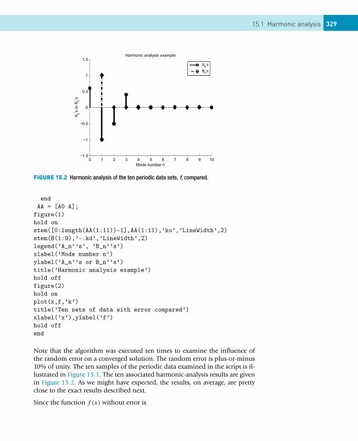
15.1 Harmonic analysis 329
FIGURE 15.2 Harmonic analysis of the ten periodic data sets, f, compared.
endAA = [A0 A];
figure(1)hold onstem([0:length(AA(1:11))-1],AA(1:11),’ko’,’LineWidth’,2)stem(B(1:9),’-.kd’,’LineWidth’,2)legend(’A_n’’s’, ’B_n’’s’)xlabel(’Mode number n’)ylabel(’A_n’’s or B_n’’s’)title(’Harmonic analysis example’)hold offfigure(2)hold onplot(x,f,’k’)title(’Ten sets of data with error compared’)xlabel(’x’),ylabel(’f’)hold offend
Note that the algorithm was executed ten times to examine the influence ofthe random error on a converged solution. The random error is plus-or-minus10% of unity. The ten samples of the periodic data examined in the script is il-lustrated in Figure 15.1. The ten associated harmonic-analysis results are givenin Figure 15.2. As we might have expected, the results, on average, are prettyclose to the exact results described next.
Since the function f (x) without error is
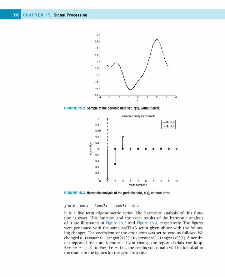
330 CHAPTER 15: Signal Processing
FIGURE 15.3 Sample of the periodic data set, f (x ), without error.
FIGURE 15.4 Harmonic analysis of the periodic data, f (x ), without error.
f = .6 − cosx − .5 cos 2x + .4 cos 3x + sinx
it is a five term trigonometric series. The harmonic analysis of this func-tion is exact. This function and the exact results of the harmonic analysisof it are illustrated in Figure 15.3 and Figure 15.4, respectively. The figureswere generated with the same MATLAB script given above with the follow-ing changes. The coefficient of the error term was set to zero as follows: Wechanged 0.1*randn(1,length(x))]; to 0*randn(1,length(x))];. Since theten repeated trials are identical, if you change the repeated-trials for loop,for ir = 1:10, to for ir = 1:1, the results you obtain will be identical tothe results in the figures for the zero error case.
15.2 Fast Fourier Transform (FFT) 331
Comparing the error-less data with the noisy data generated by adding a ran-dom error, illustrates the need for making repeated measurements in the labo-ratory to get a sensible result for the amplitudes of the harmonics that representthe shape of the phenomenon sought, viz., f (x) in the interval −π ≤ x ≤ π .Note that if a trigonometric series is used to define the input data set, the out-put of harmonic analysis yields an exact reproduction of the input series.
15.2 FAST FOURIER TRANSFORM (FFT)
James W. Cooley and John W. Tukey published An Algorithm for the MachineCalculation of Complex Fourier Series in 1965; it appeared in Mathematics ofComputations 19, 297–301. This paper was cited in the book edited by Leo L. Be-ranek and István L. Vér titled Noise and Vibration Control Engineering publishedby John Wiley & Sons (1992). This book provides a good review of signal pro-cessing as well as its practical applications in noise and vibration engineering.The discussion to follow follows closely the discussion in this book.
The Fourier transform of a time history signal, y(t), that is measured over thetime interval 0 ≤ t ≤ T is defined for all frequencies, both positive and nega-tive, by
Y(ω,T ) =T∫
0
y(t)e−i2πωt dt (15.11)
where Y is a function of frequency, ω. In terms of a digital time series of N
data values where y(t) = y(n�t), n = 0, 1, 2, . . ., N − 1. The Fourier transformmay be written as a complex Fourier series
Y(ω,T ) = Y(k�ω,N) = �t
N−1∑n=0
y(n�t) exp(−i2πωn�t) (15.12)
where the spectral components, i.e., the Y(k�ω,N)s, are generally complexvalued and are defined only at N discrete frequencies
ωk = k�ω = k
N �t, k = 0,1,2, . . . ,N − 1
Hence, this is essentially the complex version of the Fourier series expansionintroduced in the introduction of this chapter. To clarify this point further, letus divide Equation (15.12) by T = N�t . This yields the following result:
Ck = Y(k�ω,N)
N�t= 1
N
N−1∑n=0
x(n�t) exp(−i2πωn�t)
= 1
N
N−1∑n=0
x(n�t) exp(−i2πk n/N) (15.13)

332 CHAPTER 15: Signal Processing
Note the analogy between this formula and the formulas for the Fourier coeffi-cients given in the previous section on harmonic analysis. In this case, however,the coefficients are complex numbers. Since MATLAB deals with complex num-bers and does complex arithmetic, applying the FFT methodology to examinesignals is reasonably straightforward. This will be illustrated below by an ex-ample.
The complex Fourier coefficients defined by Equation (15.13) are for an as-sumed periodic function and, hence, the time history y(t) is assumed to repeatover periods equal to the sampling period, T . The Fourier components areunique only out to k = N/2, i.e., out to the frequency ωk = 1/(2�t), com-monly known as the Nyquist frequency, ωN , of the digital signal. At this fre-quency there are only two sample values per cycle and, hence, the error knownas aliasing is initiated; for details see, e.g., Beranek and Vér (1992) cited above.The first N/2+1 Fourier coefficients, from k = 0 to k = N/2, define the spectralcomponents (i.e., magnitudes of the Fourier coefficients of significant magni-tude) at positive frequencies, while the last N/2 − 1 Fourier coefficients, fromk = N/2 + 1 to k = N − 1, define the spectral components at negative frequen-cies.
The various FFT algorithms developed since the publication of Cooley-Tukeyalgorithm are well documented in the technical literature. The details of de-veloping and FFT algorithm is also beyond the scope of this presentation.However, since the procedure applied in the example examined in this sectioncan be applied to other problems that may be of interest to the reader, a few ofthe hints that need to be considered in applying the Cooley-Tukey algorithmpointed out by Beranek and Vér are worth noting since this algorithm is thebasis for the FFT algorithm applied in the example discussed in this section.They are:
� It is useful to restrict the number of equally spaced data points for each FFTto a power of 2, i.e., N = 2p , where p = 8 to 12 are commonly used.
� The frequency resolution of the Fourier components will be 1/(N �t).� The Nyquist frequency where aliasing is initiated occurs at k = N/2 and it is
ωN = 1/(2�t). The sampling frequency should be at least twice the highestfrequency expected to be found in the signal.
� The first N/2 + 1 Fourier components up to the Nyquist frequency arerelated to the last N/2 − 1 components above the Nyquist frequency byY(k) = Y ∗(N − k), k = 0, 1, 2, . . . , N − 1, where the asterisk denotes com-plex conjugate.
� The Fourier components that define only the positive frequencies is calleda one-sided spectrum. This spectrum is given by Y(0), Y(N/2), and 2Y(k),k = 1, 2, . . . , N/2 − 1.
The one-sided spectral components for a periodic signal with zero mean aregiven by
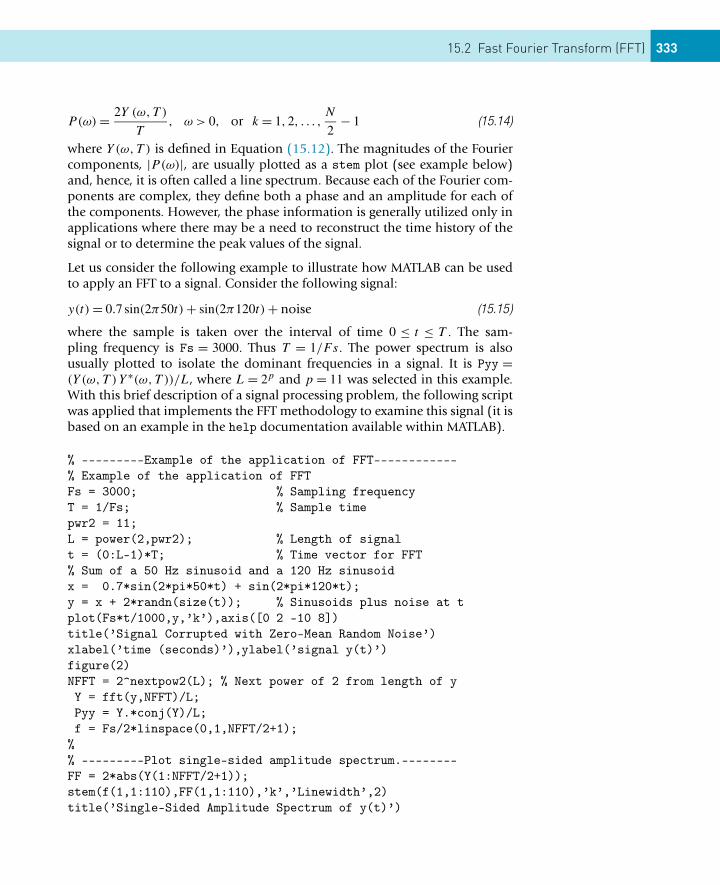
15.2 Fast Fourier Transform (FFT) 333
P(ω) = 2Y (ω,T )
T, ω > 0, or k = 1,2, . . . ,
N
2− 1 (15.14)
where Y(ω,T ) is defined in Equation (15.12). The magnitudes of the Fouriercomponents, |P(ω)|, are usually plotted as a stem plot (see example below)and, hence, it is often called a line spectrum. Because each of the Fourier com-ponents are complex, they define both a phase and an amplitude for each ofthe components. However, the phase information is generally utilized only inapplications where there may be a need to reconstruct the time history of thesignal or to determine the peak values of the signal.
Let us consider the following example to illustrate how MATLAB can be usedto apply an FFT to a signal. Consider the following signal:
y(t) = 0.7 sin(2π50t) + sin(2π120t) + noise (15.15)
where the sample is taken over the interval of time 0 ≤ t ≤ T . The sam-pling frequency is Fs = 3000. Thus T = 1/Fs. The power spectrum is alsousually plotted to isolate the dominant frequencies in a signal. It is Pyy =(Y (ω,T )Y ∗(ω,T ))/L, where L = 2p and p = 11 was selected in this example.With this brief description of a signal processing problem, the following scriptwas applied that implements the FFT methodology to examine this signal (it isbased on an example in the help documentation available within MATLAB).
% ---------Example of the application of FFT------------% Example of the application of FFTFs = 3000; % Sampling frequencyT = 1/Fs; % Sample timepwr2 = 11;L = power(2,pwr2); % Length of signalt = (0:L-1)*T; % Time vector for FFT% Sum of a 50 Hz sinusoid and a 120 Hz sinusoidx = 0.7*sin(2*pi*50*t) + sin(2*pi*120*t);y = x + 2*randn(size(t)); % Sinusoids plus noise at tplot(Fs*t/1000,y,’k’),axis([0 2 -10 8])title(’Signal Corrupted with Zero-Mean Random Noise’)xlabel(’time (seconds)’),ylabel(’signal y(t)’)figure(2)NFFT = 2^nextpow2(L); % Next power of 2 from length of yY = fft(y,NFFT)/L;Pyy = Y.*conj(Y)/L;f = Fs/2*linspace(0,1,NFFT/2+1);
%% ---------Plot single-sided amplitude spectrum.--------FF = 2*abs(Y(1:NFFT/2+1));stem(f(1,1:110),FF(1,1:110),’k’,’Linewidth’,2)title(’Single-Sided Amplitude Spectrum of y(t)’)
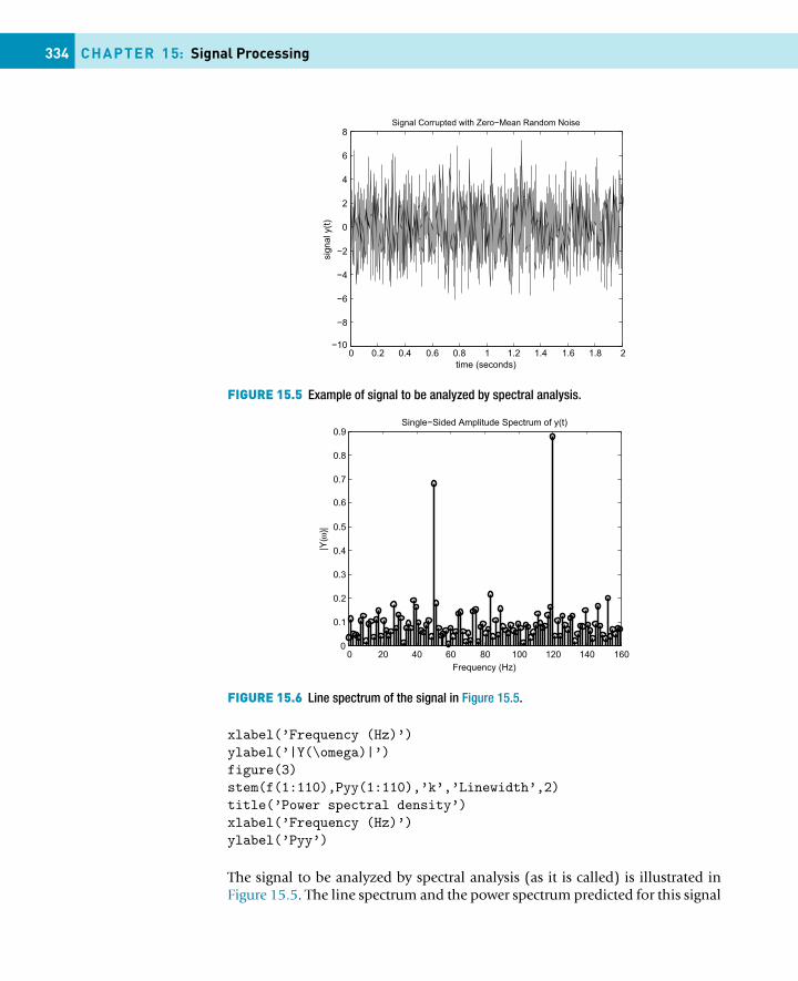
334 CHAPTER 15: Signal Processing
FIGURE 15.5 Example of signal to be analyzed by spectral analysis.
FIGURE 15.6 Line spectrum of the signal in Figure 15.5.
xlabel(’Frequency (Hz)’)ylabel(’|Y(\omega)|’)figure(3)stem(f(1:110),Pyy(1:110),’k’,’Linewidth’,2)title(’Power spectral density’)xlabel(’Frequency (Hz)’)ylabel(’Pyy’)
The signal to be analyzed by spectral analysis (as it is called) is illustrated inFigure 15.5. The line spectrum and the power spectrum predicted for this signal
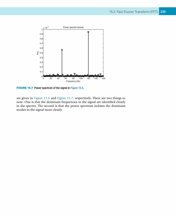
15.2 Fast Fourier Transform (FFT) 335
FIGURE 15.7 Power spectrum of the signal in Figure 15.5.
are given in Figure 15.6 and Figure 15.7, respectively. There are two things tonote. One is that the dominant frequencies in the signal are identified clearlyin the spectra. The second is that the power spectrum isolates the dominantmodes in the signal more clearly.
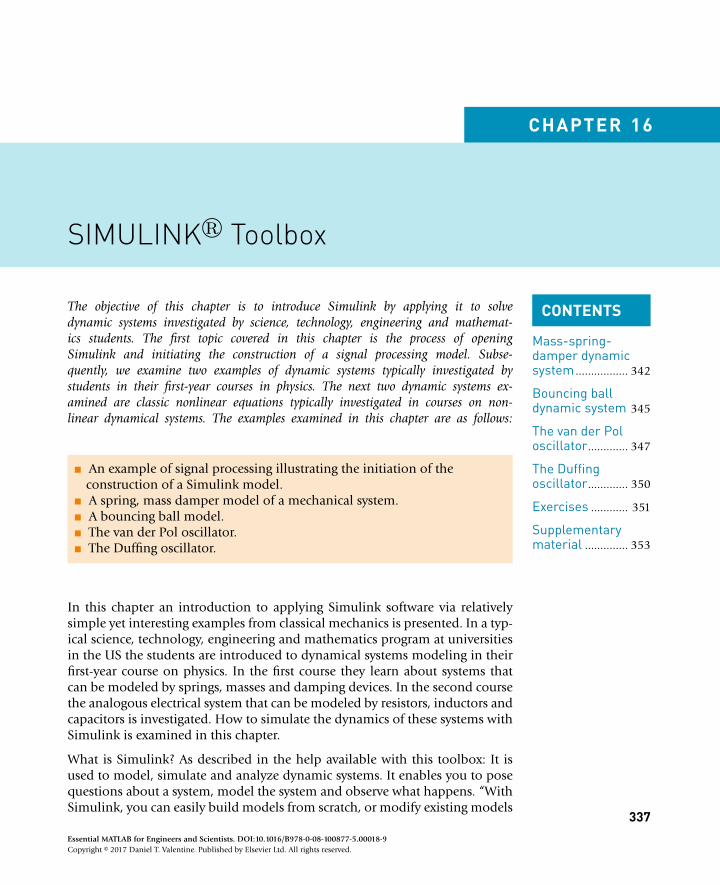
CONTENTS
Mass-spring-damper dynamicsystem ................. 342
Bouncing balldynamic system 345
The van der Poloscillator............. 347
The Duffingoscillator............. 350
Exercises ............ 351
Supplementarymaterial .............. 353
CHAPTER 16
SIMULINK� Toolbox
The objective of this chapter is to introduce Simulink by applying it to solvedynamic systems investigated by science, technology, engineering and mathemat-ics students. The first topic covered in this chapter is the process of openingSimulink and initiating the construction of a signal processing model. Subse-quently, we examine two examples of dynamic systems typically investigated bystudents in their first-year courses in physics. The next two dynamic systems ex-amined are classic nonlinear equations typically investigated in courses on non-linear dynamical systems. The examples examined in this chapter are as follows:
� An example of signal processing illustrating the initiation of theconstruction of a Simulink model.
� A spring, mass damper model of a mechanical system.� A bouncing ball model.� The van der Pol oscillator.� The Duffing oscillator.
In this chapter an introduction to applying Simulink software via relativelysimple yet interesting examples from classical mechanics is presented. In a typ-ical science, technology, engineering and mathematics program at universitiesin the US the students are introduced to dynamical systems modeling in theirfirst-year course on physics. In the first course they learn about systems thatcan be modeled by springs, masses and damping devices. In the second coursethe analogous electrical system that can be modeled by resistors, inductors andcapacitors is investigated. How to simulate the dynamics of these systems withSimulink is examined in this chapter.
What is Simulink? As described in the help available with this toolbox: It isused to model, simulate and analyze dynamic systems. It enables you to posequestions about a system, model the system and observe what happens. “WithSimulink, you can easily build models from scratch, or modify existing models
337Essential MATLAB for Engineers and Scientists. DOI:10.1016/B978-0-08-100877-5.00018-9Copyright © 2017 Daniel T. Valentine. Published by Elsevier Ltd. All rights reserved.
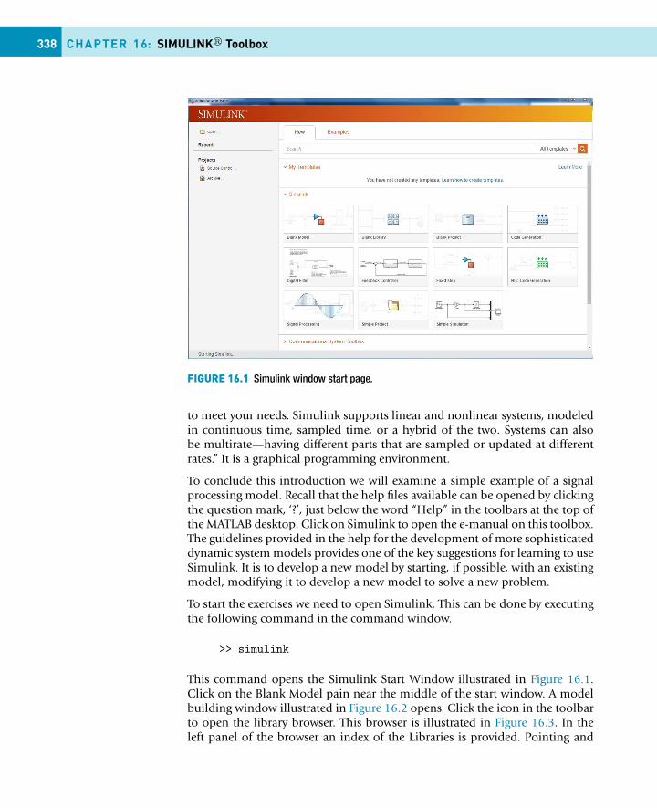
338 CHAPTER 16: SIMULINK� Toolbox
FIGURE 16.1 Simulink window start page.
to meet your needs. Simulink supports linear and nonlinear systems, modeledin continuous time, sampled time, or a hybrid of the two. Systems can alsobe multirate—having different parts that are sampled or updated at differentrates.” It is a graphical programming environment.
To conclude this introduction we will examine a simple example of a signalprocessing model. Recall that the help files available can be opened by clickingthe question mark, ‘?’, just below the word “Help” in the toolbars at the top ofthe MATLAB desktop. Click on Simulink to open the e-manual on this toolbox.The guidelines provided in the help for the development of more sophisticateddynamic system models provides one of the key suggestions for learning to useSimulink. It is to develop a new model by starting, if possible, with an existingmodel, modifying it to develop a new model to solve a new problem.
To start the exercises we need to open Simulink. This can be done by executingthe following command in the command window.
>> simulink
This command opens the Simulink Start Window illustrated in Figure 16.1.Click on the Blank Model pain near the middle of the start window. A modelbuilding window illustrated in Figure 16.2 opens. Click the icon in the toolbarto open the library browser. This browser is illustrated in Figure 16.3. In theleft panel of the browser an index of the Libraries is provided. Pointing and
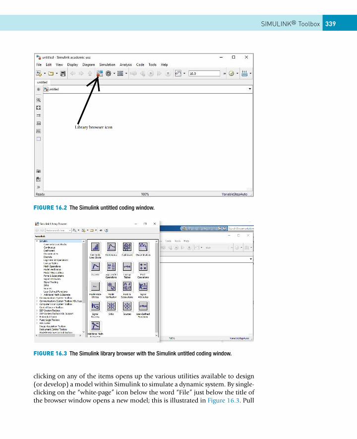
SIMULINK� Toolbox 339
FIGURE 16.2 The Simulink untitled coding window.
FIGURE 16.3 The Simulink library browser with the Simulink untitled coding window.
clicking on any of the items opens up the various utilities available to design(or develop) a model within Simulink to simulate a dynamic system. By single-clicking on the “white-page” icon below the word “File” just below the title ofthe browser window opens a new model; this is illustrated in Figure 16.3. Pull
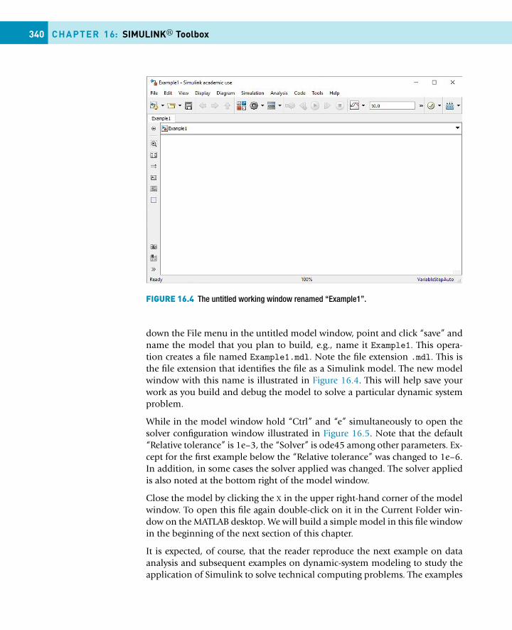
340 CHAPTER 16: SIMULINK� Toolbox
FIGURE 16.4 The untitled working window renamed “Example1”.
down the File menu in the untitled model window, point and click “save” andname the model that you plan to build, e.g., name it Example1. This opera-tion creates a file named Example1.mdl. Note the file extension .mdl. This isthe file extension that identifies the file as a Simulink model. The new modelwindow with this name is illustrated in Figure 16.4. This will help save yourwork as you build and debug the model to solve a particular dynamic systemproblem.
While in the model window hold “Ctrl” and “e” simultaneously to open thesolver configuration window illustrated in Figure 16.5. Note that the default“Relative tolerance” is 1e–3, the “Solver” is ode45 among other parameters. Ex-cept for the first example below the “Relative tolerance” was changed to 1e–6.In addition, in some cases the solver applied was changed. The solver appliedis also noted at the bottom right of the model window.
Close the model by clicking the X in the upper right-hand corner of the modelwindow. To open this file again double-click on it in the Current Folder win-dow on the MATLAB desktop. We will build a simple model in this file windowin the beginning of the next section of this chapter.
It is expected, of course, that the reader reproduce the next example on dataanalysis and subsequent examples on dynamic-system modeling to study theapplication of Simulink to solve technical computing problems. The examples
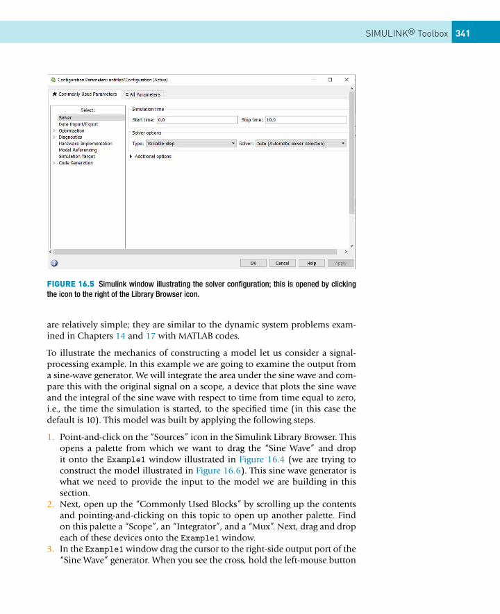
SIMULINK� Toolbox 341
FIGURE 16.5 Simulink window illustrating the solver configuration; this is opened by clickingthe icon to the right of the Library Browser icon.
are relatively simple; they are similar to the dynamic system problems exam-ined in Chapters 14 and 17 with MATLAB codes.
To illustrate the mechanics of constructing a model let us consider a signal-processing example. In this example we are going to examine the output froma sine-wave generator. We will integrate the area under the sine wave and com-pare this with the original signal on a scope, a device that plots the sine waveand the integral of the sine wave with respect to time from time equal to zero,i.e., the time the simulation is started, to the specified time (in this case thedefault is 10). This model was built by applying the following steps.
1. Point-and-click on the “Sources” icon in the Simulink Library Browser. Thisopens a palette from which we want to drag the “Sine Wave” and dropit onto the Example1 window illustrated in Figure 16.4 (we are trying toconstruct the model illustrated in Figure 16.6). This sine wave generator iswhat we need to provide the input to the model we are building in thissection.
2. Next, open up the “Commonly Used Blocks” by scrolling up the contentsand pointing-and-clicking on this topic to open up another palette. Findon this palette a “Scope”, an “Integrator”, and a “Mux”. Next, drag and dropeach of these devices onto the Example1 window.
3. In the Example1 window drag the cursor to the right-side output port of the“Sine Wave” generator. When you see the cross, hold the left-mouse button
342 CHAPTER 16: SIMULINK� Toolbox
down and drag the cross to the top-left input port of the “Mux”. This is oneway to connect a “wire” from one device to the next.
4. Following the same procedure connect the right-side port of the “Mux” tothe left-side input port of the “Scope”.
5. Starting at the left-side input port of the “Integrator” hold the left-mousebutton down and move to any location on the wire already connecting the“Sine Wave” generator to the “Mux”.
6. Finally, connect the right-side output port of the “Integrator” to the lower-left input port of the “Mux”.
7. Pull down the file menu and click “save” to save your work. In this examplewe already saved the name of this file, viz., Example1.mdl.
8. To continue, double click on the “Scope” to open the Scope window.9. Finally, click on the model window to make sure it is in the forefront. To
start the simulation hold the keys “Ctrl” and “T” down simultaneously.
You should see two curves appear on the scope. It will be the sine wave (yellow)and the integral of the sine wave (magenta). The “Mux” allows for two inputsinto the scope. The model and the results of its execution are illustrated inFigure 16.6.
Of course, if you haven’t had any experience with experimental equipmentlike oscilloscopes, sine-wave generators, multiplexers and the like, much ofthis may seem a bit mysterious. In addition, the exercise above is only a look-see exercise. It hardly demonstrates the many more powerful features availablewithin Simulink. However, more experience in your technical training and ed-ucation will allow you to explore more productively this powerful tool andclear up many of these matters. In addition, learning more about Simulinkby exercising many of the examples described in the help documentation willhelp to understand the other toolboxes, e.g., the Control Systems Toolbox.Furthermore, in courses on Dynamical Systems in mechanical and in electricalengineering, many of the available textbooks ask the student to apply Simulinkto investigate the systems examined. Thus, there are numerous sources withsample applications, including searching the computer web, that should provebeneficial in learning how to apply this tool to solve more substantial prob-lems in engineering and science. Additional details on the various utilitiesapplied in the above example can be found in the help. We next examine oneof the simplest yet quite useful dynamic system.
16.1 MASS-SPRING-DAMPER DYNAMIC SYSTEM
The simplest ordinary differential equation that can be used to investigate theoscillation of a dynamic system is the following differential equation:
d2x
dt2+ b
dx
dt+ ω2
ox = A sin(ωt). (16.1)
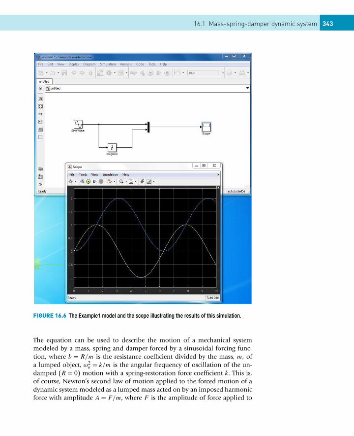
16.1 Mass-spring-damper dynamic system 343
FIGURE 16.6 The Example1 model and the scope illustrating the results of this simulation.
The equation can be used to describe the motion of a mechanical systemmodeled by a mass, spring and damper forced by a sinusoidal forcing func-tion, where b = R/m is the resistance coefficient divided by the mass, m, ofa lumped object, ω2
o = k/m is the angular frequency of oscillation of the un-damped (R = 0) motion with a spring-restoration force coefficient k. This is,of course, Newton’s second law of motion applied to the forced motion of adynamic system modeled as a lumped mass acted on by an imposed harmonicforce with amplitude A = F/m, where F is the amplitude of force applied to
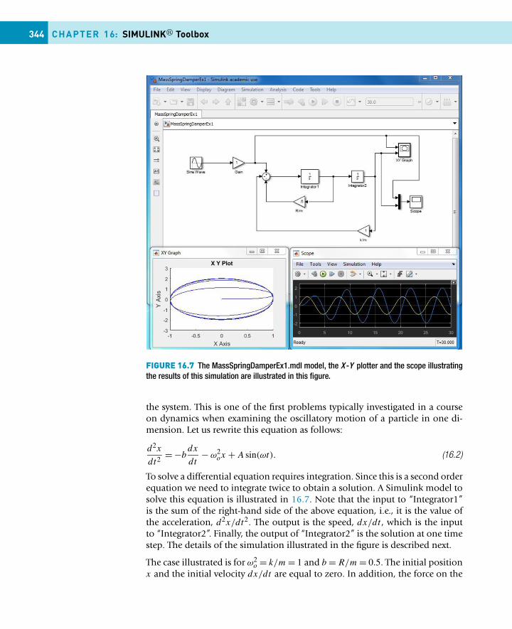
344 CHAPTER 16: SIMULINK� Toolbox
FIGURE 16.7 The MassSpringDamperEx1.mdl model, the X -Y plotter and the scope illustratingthe results of this simulation are illustrated in this figure.
the system. This is one of the first problems typically investigated in a courseon dynamics when examining the oscillatory motion of a particle in one di-mension. Let us rewrite this equation as follows:
d2x
dt2= −b
dx
dt− ω2
ox + A sin(ωt). (16.2)
To solve a differential equation requires integration. Since this is a second orderequation we need to integrate twice to obtain a solution. A Simulink model tosolve this equation is illustrated in 16.7. Note that the input to “Integrator1”is the sum of the right-hand side of the above equation, i.e., it is the value ofthe acceleration, d2x/dt2. The output is the speed, dx/dt , which is the inputto “Integrator2”. Finally, the output of “Integrator2” is the solution at one timestep. The details of the simulation illustrated in the figure is described next.
The case illustrated is for ω2o = k/m = 1 and b = R/m = 0.5. The initial position
x and the initial velocity dx/dt are equal to zero. In addition, the force on the
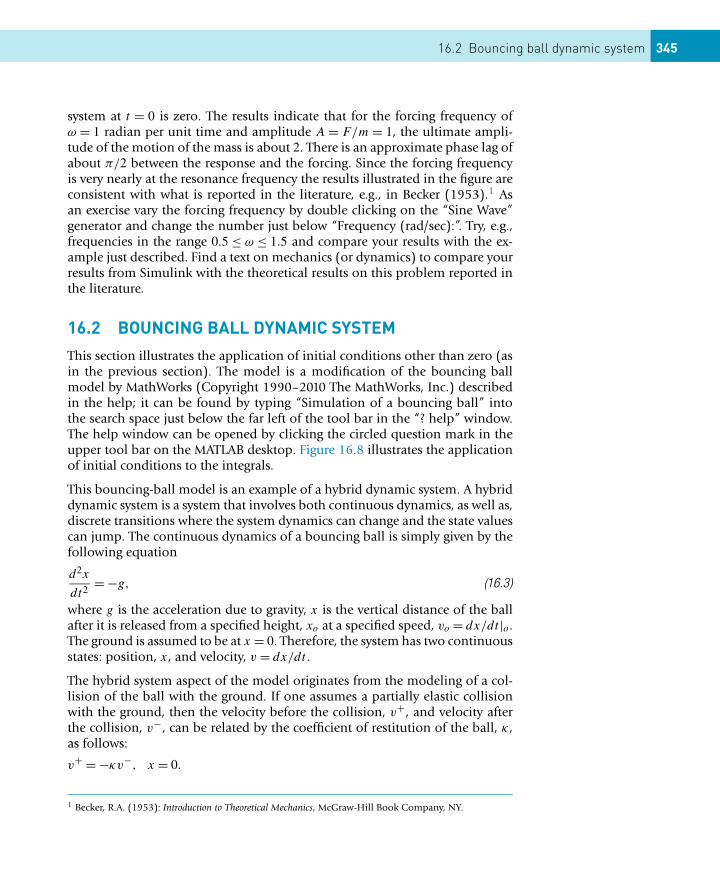
16.2 Bouncing ball dynamic system 345
system at t = 0 is zero. The results indicate that for the forcing frequency ofω = 1 radian per unit time and amplitude A = F/m = 1, the ultimate ampli-tude of the motion of the mass is about 2. There is an approximate phase lag ofabout π/2 between the response and the forcing. Since the forcing frequencyis very nearly at the resonance frequency the results illustrated in the figure areconsistent with what is reported in the literature, e.g., in Becker (1953).1 Asan exercise vary the forcing frequency by double clicking on the “Sine Wave”generator and change the number just below “Frequency (rad/sec):”. Try, e.g.,frequencies in the range 0.5 ≤ ω ≤ 1.5 and compare your results with the ex-ample just described. Find a text on mechanics (or dynamics) to compare yourresults from Simulink with the theoretical results on this problem reported inthe literature.
16.2 BOUNCING BALL DYNAMIC SYSTEMThis section illustrates the application of initial conditions other than zero (asin the previous section). The model is a modification of the bouncing ballmodel by MathWorks (Copyright 1990–2010 The MathWorks, Inc.) describedin the help; it can be found by typing “Simulation of a bouncing ball” intothe search space just below the far left of the tool bar in the “? help” window.The help window can be opened by clicking the circled question mark in theupper tool bar on the MATLAB desktop. Figure 16.8 illustrates the applicationof initial conditions to the integrals.
This bouncing-ball model is an example of a hybrid dynamic system. A hybriddynamic system is a system that involves both continuous dynamics, as well as,discrete transitions where the system dynamics can change and the state valuescan jump. The continuous dynamics of a bouncing ball is simply given by thefollowing equation
d2x
dt2= −g, (16.3)
where g is the acceleration due to gravity, x is the vertical distance of the ballafter it is released from a specified height, xo at a specified speed, vo = dx/dt |o.The ground is assumed to be at x = 0. Therefore, the system has two continuousstates: position, x, and velocity, v = dx/dt .
The hybrid system aspect of the model originates from the modeling of a col-lision of the ball with the ground. If one assumes a partially elastic collisionwith the ground, then the velocity before the collision, v+, and velocity afterthe collision, v−, can be related by the coefficient of restitution of the ball, κ ,as follows:
v+ = −κv−, x = 0.
1 Becker, R.A. (1953): Introduction to Theoretical Mechanics, McGraw-Hill Book Company, NY.
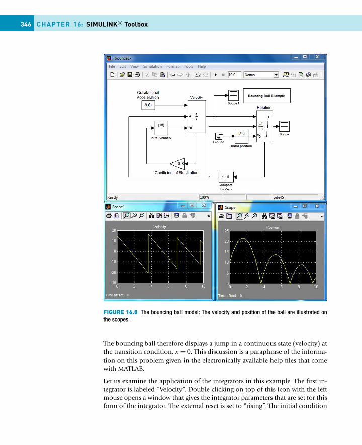
346 CHAPTER 16: SIMULINK� Toolbox
FIGURE 16.8 The bouncing ball model: The velocity and position of the ball are illustrated onthe scopes.
The bouncing ball therefore displays a jump in a continuous state (velocity) atthe transition condition, x = 0. This discussion is a paraphrase of the informa-tion on this problem given in the electronically available help files that comewith MATLAB.
Let us examine the application of the integrators in this example. The first in-tegrator is labeled “Velocity”. Double clicking on top of this icon with the leftmouse opens a window that gives the integrator parameters that are set for thisform of the integrator. The external reset is set to “rising”. The initial condition
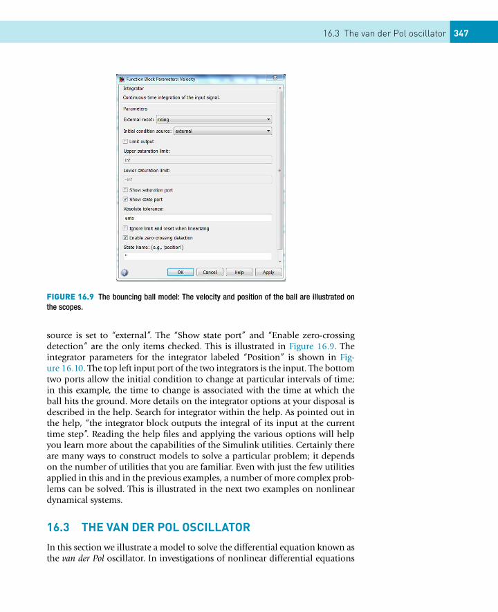
16.3 The van der Pol oscillator 347
FIGURE 16.9 The bouncing ball model: The velocity and position of the ball are illustrated onthe scopes.
source is set to “external”. The “Show state port” and “Enable zero-crossingdetection” are the only items checked. This is illustrated in Figure 16.9. Theintegrator parameters for the integrator labeled “Position” is shown in Fig-ure 16.10. The top left input port of the two integrators is the input. The bottomtwo ports allow the initial condition to change at particular intervals of time;in this example, the time to change is associated with the time at which theball hits the ground. More details on the integrator options at your disposal isdescribed in the help. Search for integrator within the help. As pointed out inthe help, “the integrator block outputs the integral of its input at the currenttime step”. Reading the help files and applying the various options will helpyou learn more about the capabilities of the Simulink utilities. Certainly thereare many ways to construct models to solve a particular problem; it dependson the number of utilities that you are familiar. Even with just the few utilitiesapplied in this and in the previous examples, a number of more complex prob-lems can be solved. This is illustrated in the next two examples on nonlineardynamical systems.
16.3 THE VAN DER POL OSCILLATOR
In this section we illustrate a model to solve the differential equation known asthe van der Pol oscillator. In investigations of nonlinear differential equations
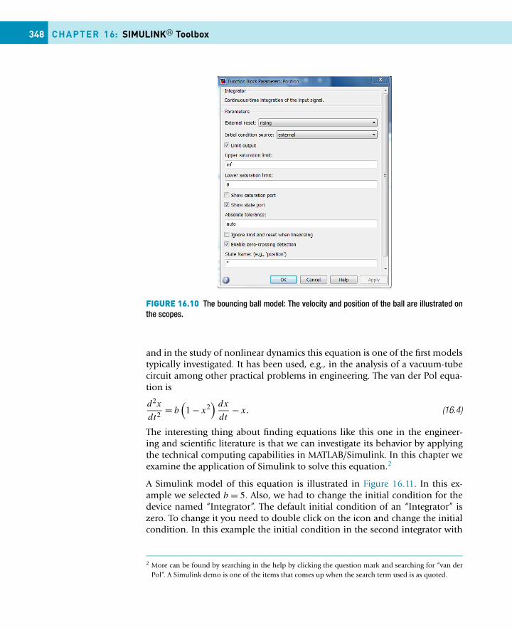
348 CHAPTER 16: SIMULINK� Toolbox
FIGURE 16.10 The bouncing ball model: The velocity and position of the ball are illustrated onthe scopes.
and in the study of nonlinear dynamics this equation is one of the first modelstypically investigated. It has been used, e.g., in the analysis of a vacuum-tubecircuit among other practical problems in engineering. The van der Pol equa-tion is
d2x
dt2= b
(1 − x2
) dx
dt− x. (16.4)
The interesting thing about finding equations like this one in the engineer-ing and scientific literature is that we can investigate its behavior by applyingthe technical computing capabilities in MATLAB/Simulink. In this chapter weexamine the application of Simulink to solve this equation.2
A Simulink model of this equation is illustrated in Figure 16.11. In this ex-ample we selected b = 5. Also, we had to change the initial condition for thedevice named “Integrator”. The default initial condition of an “Integrator” iszero. To change it you need to double click on the icon and change the initialcondition. In this example the initial condition in the second integrator with
2 More can be found by searching in the help by clicking the question mark and searching for “van derPol”. A Simulink demo is one of the items that comes up when the search term used is as quoted.
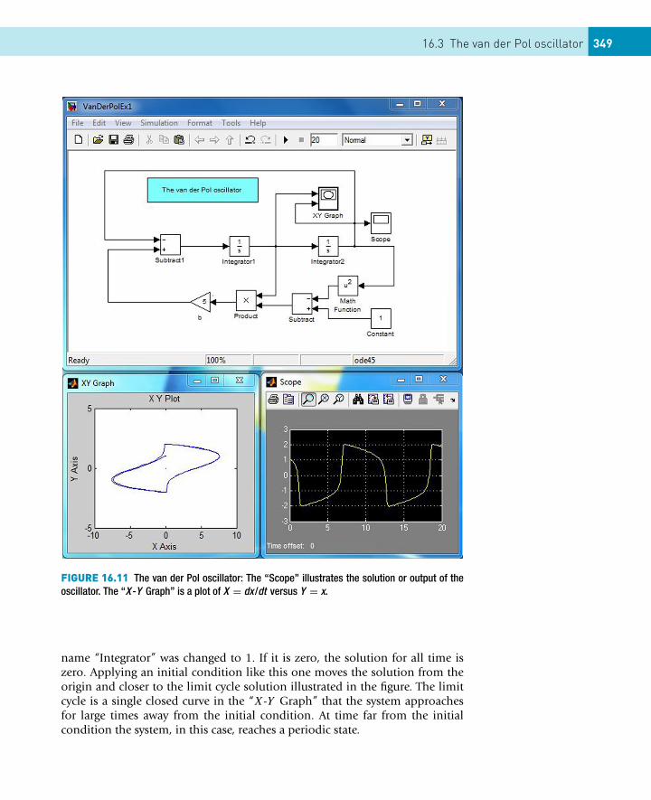
16.3 The van der Pol oscillator 349
FIGURE 16.11 The van der Pol oscillator: The “Scope” illustrates the solution or output of theoscillator. The “X -Y Graph” is a plot of X = dx/dt versus Y = x.
name “Integrator” was changed to 1. If it is zero, the solution for all time iszero. Applying an initial condition like this one moves the solution from theorigin and closer to the limit cycle solution illustrated in the figure. The limitcycle is a single closed curve in the “X-Y Graph” that the system approachesfor large times away from the initial condition. At time far from the initialcondition the system, in this case, reaches a periodic state.
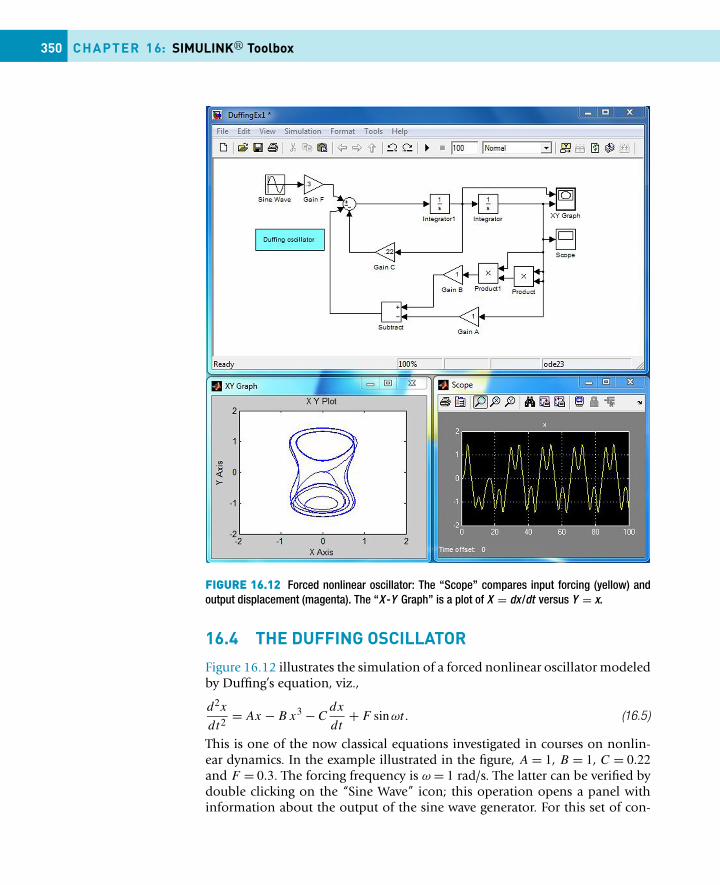
350 CHAPTER 16: SIMULINK� Toolbox
FIGURE 16.12 Forced nonlinear oscillator: The “Scope” compares input forcing (yellow) andoutput displacement (magenta). The “X -Y Graph” is a plot of X = dx/dt versus Y = x.
16.4 THE DUFFING OSCILLATOR
Figure 16.12 illustrates the simulation of a forced nonlinear oscillator modeledby Duffing’s equation, viz.,
d2x
dt2= Ax − B x3 − C
dx
dt+ F sinωt. (16.5)
This is one of the now classical equations investigated in courses on nonlin-ear dynamics. In the example illustrated in the figure, A = 1, B = 1, C = 0.22and F = 0.3. The forcing frequency is ω = 1 rad/s. The latter can be verified bydouble clicking on the “Sine Wave” icon; this operation opens a panel withinformation about the output of the sine wave generator. For this set of con-
16.4 Exercises 351
stants the phase portrait, the X-Y graph in the figure, evolves into a limit cycleor periodic orbit called a “stable period 3 orbit” as described in detail in thebook by Guckenheimer and Holmes.3 This example, like the others presentedin this chapter, are intended to illustrate that you can study the properties ofthe solutions to differential equations numerically relatively easily by applyingthe tools in Simulink (and in MATLAB).
There is a wealth of literature on the theory and the numerics of nonlinearequations and, in particular, the Duffing and the van der Pol equations. Thetheoretical results reported in Guckenheimer and Holmes helped the authorselect the constants applied in this example. Suggestions for changes in theconstants are to be examined in the exercises at the end of this chapter.
EXERCISES16.1 Reproduce the signal processing model, i.e., first example in this chap-
ter on the display of the sine and its integral. Execute the simulationto make sure it works (i.e., compares favorably with the results in theexample). Next, do the following:(a) Double click on the integrator and change the initial condition
from 0 to 1. Apply the change by clicking the button in the lowerright corner of the integrator function block. Execute the simula-tion. What is the maximum value of the integral? What is the mini-mum value of the integral?
(b) Double click on the sine wave icon and change the frequency from1 to 2 and the amplitude from 1 to 2. Apply the changes by clickingthe button in the lower right corner of the sine wave source block.Execute the simulation. Note that the frequency is doubled and theamplitude is doubled.
(c) Change the phase of the sine wave from 0 to π/2. Make sure thatthe amplitude and frequency are set equal to 1. Apply the changesand execute the simulation. Note that the input function is a cosineinstead of a sine function.
16.2 Reproduce the bouncing-ball model and execute it to determine thatyour reproduction is consistent with the example in this chapter. Witha working code examine changes in the coefficient of restitution. Con-sider several values in the range 0.5 ≤ κ ≤ 0.9. Also examine changes inthe initial conditions for κ = 0.8. To change the value of κ you need todouble click on the icon for the coefficient of restitution, change its valueand apply it. The same is done to change the initial velocity or the ini-tial position. Once you examine a few different cases explain what youfound.
3 Guckenheimer, John, & Philip Holmes (1983): Nonlinear Oscillations, Dynamical Systems, and Bifurca-tions of Vector Fields, Springer-Verlag, NY.
352 CHAPTER 16: SIMULINK� Toolbox
16.3 Reproduce the model for a forced spring-mass-damper mechanical sys-tem. Remove the “X-Y Graph”, its connecting wires, the “Mux” and itsconnecting wires. Then reattach the “Scope” to the wire attached to theoutput of “Integrator2”. The model is the spring-mass-damper modelwith a step change in the force applied at t = 0 as can be verified bydouble clicking on the “Step” icon; change the “Step time” from thedefault value of 1 to zero if the time the step is applied is not equalto zero. Set the resistance coefficient R/m to zero. Leave k/m = 1, i.e.,the spring constant coefficient. Execute the simulation. What is the fre-quency of oscillation? Examine R/m = .25, 1, 2 and 4 to determine theeffect of increased damping on the solution. If you look this problem upin a physics book on mechanics it is usually under the topic “dampedharmonic oscillator”. If R/m = 0, it is the harmonic oscillator solutionknown as simple-harmonic motion; this should have been the solutionthat you found as part of the examination of the dynamic system in thisproblem. Without damping (i.e., R = 0) the solution is a sinusoidal mo-tion with constant amplitude. The frequency of oscillation is the naturalfrequency, ωo = √
k/m = 1 in this case. Thus, it is not unexpected that acycle of oscillation occurs over a time interval of 2π ; review your resultsto make sure that this is the case. If ω2 = (R/m)2/2, then the motion iscritically damped. This means that the dynamic system reaches its infi-nite time, constant valued solution without overshoot. If ωo is less thanthis value, the system is said to be underdamped. If ωo is greater thanthis value, the system is said to be overdamped. Setting R/m = 2 leads toa critically damped behavior. Describe, from your solutions for the rangeof R/m considered in this problem, the meaning of underdamped, crit-ically damped and overdamped response (as reflected in the solution x)of the system for the mechanical system examined in this problem.
16.4 In the previous problem try the damping coefficient R/m = −0.25. De-scribe the results. Notice how the amplitude grows with time. Thus, witha negative resistance coefficient we have growth in the amplitude of thesolution. If you set k/m = 0, you can investigate exponential growth.Create a problem that you provide a solution that deals with the prob-lem of exponential growth.
16.5 Reproduce the van der Pol oscillator model. Execute the simulation tocompare your results with the results in the example (this is, of course,a necessary step to check your computer code). Next, set the dampingcoefficient b = 0. Execute the simulation. The result should be simple-harmonic motion of amplitude unity because the initial condition in thesecond integrator was set equal to unity and period equal to 2π . Next,examine the case for b = 1. Finally, examine b = 5. Note the qualitativechanges in the response function, i.e., in the plotted values of x.
16.6 Reproduce the Duffing oscillator model. Execute the simulation to com-pare your results with the results in the example. Set the parameters
16.A Supplementary material 353
A = B = 0. The result is forced harmonic motion at a single frequency.Try examining the linear case, which means B = 0, and −1 ≤ A ≤ −0.1,which means a spring. In all cases the motion ends up being a forcedharmonic motion of a single sinusoidal frequency. This is because thecubic-nonlinear term was suppressed by setting B = 0. (There are manyother combinations that you can explore. However, be aware of the factthat some combinations of parameters lead to chaotic solutions and,hence, may never settle down to a periodic state. There also may be pa-rameter selections that lead to unstable solutions.)
APPENDIX 16.A SUPPLEMENTARY MATERIAL
Supplementary material related to this chapter can be found online athttp://dx.doi.org/10.1016/B978-0-08-100877-5.00018-9.
CONTENTS
Algebra................ 356Polynomials........... 357Vectors................... 359Matrices ................ 360
Calculus .............. 363
Laplace and Ztransforms ......... 366
Generalizedfunctions ............. 367
Differentialequations ............ 369
Implementation offuntool, MuPAD andhelp ...................... 370The funtool ............ 370The MuPAD notebook∗and Symbolic help . 370
Exercises ............ 373
CHAPTER 17
Symbolics Toolbox
The objective of this chapter is to introduce the Symbolic tools available within MAT-LAB. It is a useful set of tools for the application of mathematics in science and en-gineering. Examples of the application of the Symbolic capabilities have already beengiven elsewhere in this book to check analytic solutions found in the literature. In addi-tion, predictions based on the analytic solutions were compared with predictions basedon computational methods. The symbolic mathematical tools covered in this chapterare:
� Algebra: Polynomials, vectors and matrices.� Calculus: Differentiation and integration.� Transforms: Laplace and Z transforms.� Generalized functions: Heaviside and Dirac.� Systems of ordinary differential equations.� The funtool, MuPAD and help.
With the Symbolics toolbox MATLAB can be considered the “mathematicalhandbook” for the students of the 21st century. In the old days science andengineering students were required to purchase a “standard” mathematicshandbook. Today, there are very few students, if any, who own and use a math-ematics handbook. The computer and tools like MATLAB have changed thissituation in a positive way. However, as for the second author of this book, ithas been an interesting exercise to demonstrate that MATLAB is this century’shandbook. In this chapter an introduction to the application of Symbolicsfollows a procedure based on a review of handbook information and provid-ing examples for the kinds of information we were expected to look up in ahandbook and, hence, what we, sort of, expect students to find by applyingcomputer tools like MATLAB.
The main problem, if it is a problem at all, in the application of the symbolictoolbox, or any other computer tool that allows the user to do symbolic anal-
355Essential MATLAB for Engineers and Scientists. DOI:10.1016/B978-0-08-100877-5.00019-0Copyright © 2017 Daniel T. Valentine. Published by Elsevier Ltd. All rights reserved.
356 CHAPTER 17: Symbolics Toolbox
ysis, is that to use the tool effectively you need to know something about themathematical questions being raised. In other words, if you want to differ-entiate the function, f (x), with respect to the variable x, you need to knowthe meaning of a function and the meaning of differentiation or finding thederivative of f with respect to x, viz., finding df/dx.
Another example is finding the solutions of a quadratic equation. You need toknow what kind of equation this is and the meaning of solving an algebraicequation of this type. Hence, if you know what to ask, MATLAB Symbolics canbe applied to help you find an answer to a symbolic mathematical question.
The application of symbolics to examine mathematical questions that can beanswered with the help of mathematical handbooks is addressed in this chap-ter to illustrate the power of the symbolic tools available in MATLAB. Certainlythe tools are more powerful than the relatively simple examples presented inthis chapter. Once you are adept at using this toolbox, then you can extendthe application of this toolbox to examine more difficult questions that mayeven be beyond the capabilities of more traditional applications of appliedmathematics to solve problems in science and in engineering.
The symbolic mathematical topics covered in a typical handbook are, e.g., alge-bra, trigonometry, calculus, integration, differentiation and differential equa-tions. The information provided in a handbook is to help the student, engineeror scientist make progress in solving mathematical problems they confrontin their attempts to solve technical problems. A solid education in science,technology, engineering and mathematics (STEM) provides the necessary back-ground to utilize handbooks and/or tools like MATLAB in a productive way. Ofcourse, MATLAB like handbooks need to be used regularly to gain proficiencyin applying such tools as part of finding solutions. We will touch some of thetopics covered in handbooks to help guide the readers in their attempts toapply the Symbolic toolbox within MATLAB. We will start with algebra includ-ing linear algebra, vector algebra and matrix algebra. Then we will examinedifferentiation and integration. This will be followed by investigating integraltransforms and, in particular, the Laplace transform. Then we will conclude byinvestigating the symbolic solution of differential equations.
17.1 ALGEBRA
In Section 1.1.6 we introduced how to solve a system of linear equations. Oneexample applied the solve utility available in MATLAB Symbolics. Let us ex-tend that example by solving the simultaneous system of quadratic equations
x2 + 3y = 0, y2 + 2x = 0.
Applying the same procedure illustrated in Section 1.1.6, we get the follow-ing results by typing and executing the following command in the CommandWindow. The results are also illustrated below.
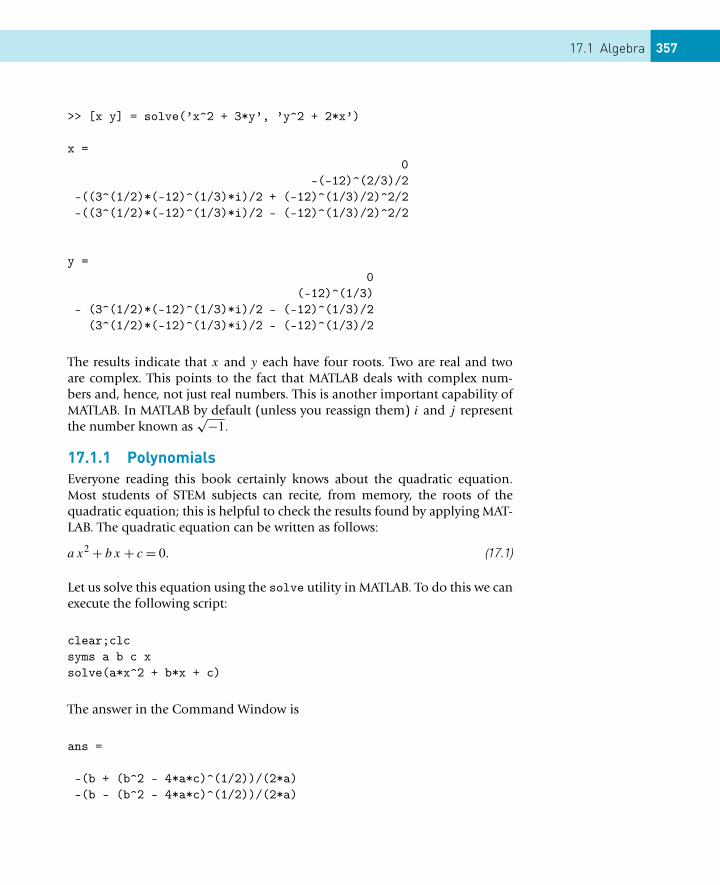
17.1 Algebra 357
>> [x y] = solve(’x^2 + 3*y’, ’y^2 + 2*x’)
x =0
-(-12)^(2/3)/2-((3^(1/2)*(-12)^(1/3)*i)/2 + (-12)^(1/3)/2)^2/2-((3^(1/2)*(-12)^(1/3)*i)/2 - (-12)^(1/3)/2)^2/2
y =0
(-12)^(1/3)- (3^(1/2)*(-12)^(1/3)*i)/2 - (-12)^(1/3)/2
(3^(1/2)*(-12)^(1/3)*i)/2 - (-12)^(1/3)/2
The results indicate that x and y each have four roots. Two are real and twoare complex. This points to the fact that MATLAB deals with complex num-bers and, hence, not just real numbers. This is another important capability ofMATLAB. In MATLAB by default (unless you reassign them) i and j representthe number known as
√−1.
17.1.1 PolynomialsEveryone reading this book certainly knows about the quadratic equation.Most students of STEM subjects can recite, from memory, the roots of thequadratic equation; this is helpful to check the results found by applying MAT-LAB. The quadratic equation can be written as follows:
a x2 + b x + c = 0. (17.1)
Let us solve this equation using the solve utility in MATLAB. To do this we canexecute the following script:
clear;clcsyms a b c xsolve(a*x^2 + b*x + c)
The answer in the Command Window is
ans =
-(b + (b^2 - 4*a*c)^(1/2))/(2*a)-(b - (b^2 - 4*a*c)^(1/2))/(2*a)
358 CHAPTER 17: Symbolics Toolbox
Thus, as expected, the solutions of the quadratic equation are
x = − 1
2a
(b ±
√b2 − 4ac
)(17.2)
For the two roots to be real numbers b2 ≥ 4ac. If the equality holds, then thetwo roots are equal. If b2 < 4ac the roots are complex and unequal. An alter-native one-line command can be used to solve this equation; this can be donein the Command Window as follows
>> solve(’a*x^2+b*x+c’)
The apostrophes indicate that what is between them is a symbolic expression.The output of both procedures of the application of solve is a 2 × 1 symbolicdata-type array. Since this is a quadratic equation we expect to get two solu-tions.
Next, let us examine the cubic polynomial
a x3 + b x2 + c x + d = 0. (17.3)
To find the roots of this equation we can execute the following script:
clear;clcsyms a b c d xsolve(a*x^3 + b*x^2 + c*x + d)
In this case, since we are solving a cubic, the answer (ans) is in a 3 × 1 sym-bolic data-type array. The answer is rather lengthy however and, hence, it is notreproduced here. It is produced in the command window.
Let us consider another example. Let us solve
ax4 + cx = 0.
The following commands were executed in the Command Window:
>> solve(’a*x^4 + c*x ’);>> solution = simple(ans);>> solution
solution =
0(-c/a)^(1/3)
((3^(1/2)*i - 1)*(-c/a)^(1/3))/2-((3^(1/2)*i + 1)*(-c/a)^(1/3))/2
17.1 Algebra 359
>> latex(solution)
ans =
\left(\begin{array}{c} 0\\ {\left(-\frac{c}{a}\right)}^{\frac{1}{3}}\\\frac{\left( - 1 + \sqrt{3}\, \mathrm{i}\right)\,{\left(-\frac{c}{a}\right)}^{\frac{1}{3}}}{2}\\-\frac{\left(1 + \sqrt{3}\, \mathrm{i}\right)\,{\left(-\frac{c}{a}\right)}^{\frac{1}{3}}}{2} \end{array}\right)
This answer (ans) was used in the word processor used by the second author;the word processor implements Latex. This translation to Latex gives the fol-lowing array of the four roots to this quartic equation:⎛⎜⎜⎜⎜⎜⎜⎝
0(− ca
) 13(
−1+√3 i
)(− c
a )13
2
−(
1+√3 i
)(− c
a )13
2
⎞⎟⎟⎟⎟⎟⎟⎠
Note that two of the roots are complex numbers.
Finally, let us examine the solution of three simultaneous linear equations withthe solve utility. Let us solve
x + y + z = 1, 2x + 3y + z = 1, x + y + 3z = 0.
Doing this in the Command Window, we get
>> [x y z] = solve(’x + y + z = 1’,’2*x + 3*y + z = 1’,’x + y + 3*z = 0’)
The solution of this system of equations leads to x = 3, y = −3/2 and z = −1/2.
Note that there are a variety of methods to implement the solve function(or solution procedure utility) within Symbolics. If numerical solutions areobtained, as in the last example, they need to be converted to double data typesto use them in MATLAB scripts (this was already illustrated in Section 1.1.6).
17.1.2 VectorsThe single row or single column arrays are vectors. Let us consider the following3-component vectors:
x1 = (a1, b1, c1), x2 = (a2, b2, c2)
There are two ways to multiply these mathematical objects that most of thestudents are familiar. They are the inner or dot product and the vector or crossproduct. They can be found by applying the following script of Symbolic com-mands (from the editor).
360 CHAPTER 17: Symbolics Toolbox
format compactsyms a1 a2 b1 b2 c1 c2 realx1 = [a1,b1,c1]x2 = [a2,b2,c2]x1_dot_x2 = dot(x1,x2)x1_cross_x2 = cross(x1,x2)format
The results in the Command Window are
x1 =[ a1, b1, c1]x2 =[ a2, b2, c2]x1_dot_x2 =a1*a2 + b1*b2 + c1*c2x1_cross_x2 =[ b1*c2 - b2*c1, a2*c1 - a1*c2, a1*b2 - a2*b1]
The format compact was implemented to get the compact output illustratedabove. The last command, viz., format, was implemented to reset the defaultoutput-display format in the Command Window. The solution can be writtenas follows:
x1 · x2 = a1a2 + b1b2 + c1c2
The dot product is a scalar.
x1 × x2 = (b1c2 − b2c1, a2c1 − a1c2, a1b2 − a2b1)
The cross product is a vector. It is a three-component vector (the same numberof components as the vectors that are multiplied to get this result).
17.1.3 MatricesLet us consider the following mathematical objects known as matrices. We canadd and subtract the two objects. We can multiply and divide the two objects.We will do these operations using the Symbolic toolbox
Ma =(
a11 a12a21 a22
)
Mb =(
b11 b12b21 b22
)
The following script was executed in MATLAB:
17.1 Algebra 361
format compactsyms a11 a12 a21 a22 b11 b12 b21 b22Ma = [a11 a12; a21 a22]Mb = [b11 b12; b21 b22]Msum = Ma + MbMproduct = Ma*Mb
The results in the Command Window are
Ma =[ a11, a12][ a21, a22]Mb =[ b11, b12][ b21, b22]Msum =[ a11 + b11, a12 + b12][ a21 + b21, a22 + b22]Mproduct =[ a11*b11 + a12*b21, a11*b12 + a12*b22][ a21*b11 + a22*b21, a21*b12 + a22*b22]
The addition of the two matrices involve term-by-term addition.
Ma ± Mb =(
a11 ± b11 a12 ± b12a21 ± b21 a22 ± b22
).
The product leads to a matrix of the same size as the matrices that are multi-plied; each term in the result is the multiplication of the a row of Ma times thecolumn on Mb summed together. Study the product matrix, as written below,to verify the matrix multiplication process. The product of the two matrices is
Ma Mb =(
a11 b11 + a12 b21 a11 b12 + a12 b22a21 b11 + a22 b21 a21 b12 + a22 b22
).
Let us analyze a number of properties of the following matrix:
Ma =(
c11 c12c21 c22
)
syms c11 c12 c21 c22 realMc = [c11 c12; c21 c22]Mcdet = det(Mc);Mcinv = inv(Mc);Mc*inv(Mc);disp(’ Mc * Mcinv = Imatrix’)
362 CHAPTER 17: Symbolics Toolbox
Imatrix = simple(ans)McdetMcinv[EigenVectorsMc EigenValuesMc] = eig(Mc)
Except for the eigenvectors and eigenvalues, the following output was in theCommand Window. The latter were converted to Latex and are reported below.
Mc =[ c11, c12][ c21, c22]Mc * Mcinv = ImatrixImatrix =[ 1, 0][ 0, 1]Mcdet =c11*c22 - c12*c21Mcinv =[ c22/(c11*c22 - c12*c21), -c12/(c11*c22 - c12*c21)][ -c21/(c11*c22 - c12*c21), c11/(c11*c22 - c12*c21)]
The eigenvalues associated with this matrix are(c112 + c22
2 −√
c112−2 c11 c22+c22
2+4 c12 c212 0
0 c112 + c22
2 +√
c112−2 c11 c22+c22
2+4 c12 c212
).
This is a result of diagonalizing the matrix (a process interpreted geometricallyas a rotation of the coordinate system to find the coordinates in which thematrix only has finite diagonal terms). The coordinate system at which thisoccurs is given by the orthogonal eigenvectors. The corresponding eigenvectorsfor this example are(
c112 + c22
2 −√
c112−2 c11 c22+c22
2+4 c12 c212
c21− c22
c21
c112 + c22
2 +√
c112−2 c11 c22+c22
2+4 c12 c212
c21− c22
c211 1
).
Let us next consider the analysis of a three-by-three symmetric matrix, viz.,
M =⎛⎝ a d e
d b fe f c
⎞⎠
This matrix was examined in detail by implementing the following script. It isan important mathematical object that plays an important role in, e.g., struc-tural mechanics where it is the form of the stress tensor.
17.2 Calculus 363
format compactsyms a b c d e f realM = [a d e
d b fe f c]
Mdet = det(M);Minv = inv(M);M*inv(M);disp(’ M * Minv = Imatrix’)Imatrix = simple(ans)MdetMinv[EigenVectorsM EigenValuesM] = eig(M)format
The results in the Command Window, except for the rather lengthy eigenvalue,eigenvector and inverse expressions are as follows:
M =[ a, d, e][ d, b, f][ e, f, c]M * Minv = Imatrix
Imatrix =[ 1, 0, 0][ 0, 1, 0][ 0, 0, 1]Mdet =- c*d^2 + 2*d*e*f - b*e^2 - a*f^2 + a*b*c
We know that the inverse of M is determined correctly because M M−1 = I,where I is the identity matrix. It is left as an exercise to examine the inversematrix and the results of the eigenvalue problem solved by the Symbolic toolsin MATLAB.
If the matrix represents the state of stress at a point in a solid material, theeigenvalues would be the principal stresses and the eigenvectors the principaldirections. This information is important in the analysis of the strength of ma-terials. Similar matrices appear in modeling the mechanics of fluids.
17.2 CALCULUS
In this section we examine symbolic differentiation and integration. We willdo this simultaneously because they are essentially inverse operation. Let us
364 CHAPTER 17: Symbolics Toolbox
examine the quadratic function
f = ax2 + bx + c. (17.4)
The derivative of this equation is
df
dx= 2ax + b (17.5)
This can be verified by applying the Symbolic tools in MATLAB. We can do thisas follows:
format compactsyms x a b c realf = a*x^2 + b*x + cdisp(’dfdx = diff(f,x) was executed to get:’)dfdx = diff(f,x)% Integrationdisp(’f = int(dfdx,x) was executed to get:’)f = int(dfdx,x)disp(’ Note that the constant of integration, c, is implied.’)disp(’ Hence, to include it you need to add c to f:’)f = f + cdisp(’f = expand(f) was executed to get:’)f = expand(f)disp(’ Thus, the function f is recovered (as expected).’)format
The output to the Command Window is
f =a*x^2 + b*x + cdfdx = diff(f,x) was executed to get:dfdx =b + 2*a*xf = int(dfdx,x) was executed to get:f =x*(b + a*x)Note that the constant of integration, c, is implied.Hence, to include it you need to add c to f:f =c + x*(b + a*x)f = expand(f) was executed to get:f =a*x^2 + b*x + cThus, the function f is recovered (as expected).
17.2 Calculus 365
Thus, we verified the formula for df/dx. The next step is to verify the resultsof differentiation by integrating. This was done in the script given above byexecuting int(dfdx,x). The result obtained is f to within a constant. Theintegration tool does not explicitly include the arbitrary constant of integration.Hence, a constant needs to be added as illustrated in the above example. Thenthe function f with the added constant is expanded (expand(f)), leading tothe result sought, i.e., the recovery of the original function f .
Let us examine a second example. It is the examination of
f = a sin2 x + b cosx (17.6)
Differentiating this formula and, subsequently, integrating df/dx, we get thefollowing: The script in the editor that was executed is
format compactsyms x a b c realf = a*sin(x)^2 + b*cos(x)dfdx = diff(f,x)% Integrationff = int(dfdx,x)ff = expand(ff)format
The output to the Command Window is
f =a*sin(x)^2 + b*cos(x)dfdx =2*a*cos(x)*sin(x) - b*sin(x)ff =2*(cos(x)/2 + 1/2)*(2*a + b - 2*a*(cos(x)/2 + 1/2))ff =a + b + b*cos(x) - a*cos(x)^2
Note that the result of the integration of df/dx is (it is ff in the script; it is f
below)
f = a + b + b cosx − a cos2 x
Substituting cos2 x = 1 − sin2 x, we get
f = a sin2 x + b cosx + b + c
where c is the arbitrary constant of integration. Since it is arbitrary, let us selectit as c = −b. Thus,
f = a sin2 x + b cosx
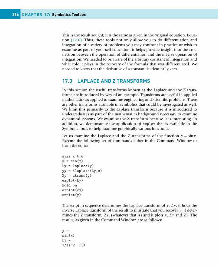
366 CHAPTER 17: Symbolics Toolbox
This is the result sought; it is the same as given in the original equation, Equa-tion (17.6). Thus, these tools not only allow you to do differentiation andintegration of a variety of problems you may confront in practice or wish toexamine as part of your self-education, it helps provide insight into the con-nection between the operation of differentiation and the inverse operation ofintegration. We needed to be aware of the arbitrary constant of integration andwhat role it plays in the recovery of the formula that was differentiated. Weneeded to know that the derivative of a constant is identically zero.
17.3 LAPLACE AND Z TRANSFORMS
In this section the useful transforms known as the Laplace and the Z trans-forms are introduced by way of an example. Transforms are useful in appliedmathematics as applied to examine engineering and scientific problems. Thereare other transforms available in Symbolics that could be investigated as well.We limit this primarily to the Laplace transform because it is introduced toundergraduates as part of the mathematics background necessary to examinedynamical systems. We examine the Z transform because it is interesting. Inaddition, we demonstrate the application of ezplot that is available in theSymbolic tools to help examine graphically various functions.
Let us examine the Laplace and the Z transforms of the function y = sinx.Execute the following set of commands either in the Command Window orfrom the editor.
syms x t wy = sin(x)Ly = laplace(y)yy = ilaplace(Ly,x)Zy = ztrans(y)ezplot(Ly)hold onezplot(Zy)ezplot(y)
The script in sequence determines the Laplace transform of y, Ly, it finds theinverse Laplace transform of the result to illustrate that you recover y, it deter-mines the Z transform, Zy, (whatever that is) and it plots y, Ly and Zy. Theresults, as given in the Command Window, are as follows:
y =sin(x)Ly =1/(s^2 + 1)
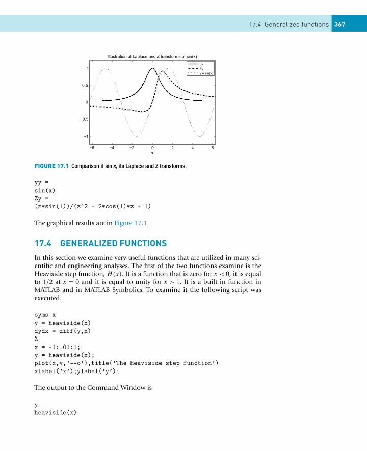
17.4 Generalized functions 367
FIGURE 17.1 Comparison if sin x, its Laplace and Z transforms.
yy =sin(x)Zy =(z*sin(1))/(z^2 - 2*cos(1)*z + 1)
The graphical results are in Figure 17.1.
17.4 GENERALIZED FUNCTIONS
In this section we examine very useful functions that are utilized in many sci-entific and engineering analyses. The first of the two functions examine is theHeaviside step function, H(x). It is a function that is zero for x < 0, it is equalto 1/2 at x = 0 and it is equal to unity for x > 1. It is a built in function inMATLAB and in MATLAB Symbolics. To examine it the following script wasexecuted.
syms xy = heaviside(x)dydx = diff(y,x)%x = -1:.01:1;y = heaviside(x);plot(x,y,’--o’),title(’The Heaviside step function’)xlabel(’x’);ylabel(’y’);
The output to the Command Window is
y =heaviside(x)
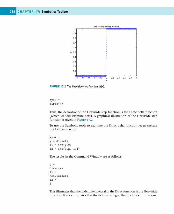
368 CHAPTER 17: Symbolics Toolbox
FIGURE 17.2 The Heaviside step function, H(x ).
dydx =dirac(x)
Thus, the derivative of the Heaviside step function is the Dirac delta function(which we will examine next). A graphical illustration of the Heaviside stepfunction is given in Figure 17.2.
To use the Symbolic tools to examine the Dirac delta function let us executethe following script:
syms xy = dirac(x)I1 = int(y,x)I2 = int(y,x,-1,1)
The results in the Command Window are as follows:
y =dirac(x)I1 =heaviside(x)I2 =1
This illustrates that the indefinite integral of the Dirac function is the Heavisidefunction. It also illustrates that the definite integral that includes x = 0 is one.
17.5 Differential equations 369
The Dirac function is infinite at x = 0 and it is zero everywhere else. It x = 0 isnot included in the range of integration the integral is zero. Note that where thedelta function is infinite and, hence, where the Heaviside step function jumpsfrom zero to one can be changed by changing the x coordinate to anotherorigin where the argument of the two functions is equal to zero.
17.5 DIFFERENTIAL EQUATIONS
The function dsolve is an ordinary differential equation and a system of or-dinary differential equation (ODE) solver. We will examine two examples inthis section. One is the solution of a single ODE and a system of ODEs. Let usexamine the equation
d3y
dx3= a x2.
To solve this equation all we need to do is to execute the following command:
>> dsolve(’D3y= a*x^2’,’x’)
The result of executing this command is
ans =(a*x^5)/60 + (C2*x^2)/2 + C3*x + C4
Thus, the solution is
a x5
60+ C1 x2
2+ C2 x + C3
where C1, C2 and C3 are the three arbitrary constants of integration. The proce-dure for solving a differential equation is to integrate. In this case because it isa third-order differential equation that we solved, it required three integrationsand, hence, the result is to within three arbitrary constants.
In the next example we solve two equations simultaneously. In addition, wespecify constraints (or boundary conditions). The equations to be solved are
df
dt= 3f + 4g,
dg
dt= −4f + 3g.
This system of equations, since it is second order, is subject to two constraints.In this example they are f (0) = 0 and g(0)− 1, which can be interpreted as ini-tial conditions. The solution can be obtained by implementing the followingcommand in MATLAB:
[f, g] = dsolve(’Df = 3*f + 4*g, Dg = -4*f + 3*g’,’f(0) = 0,g(0) = 1’)
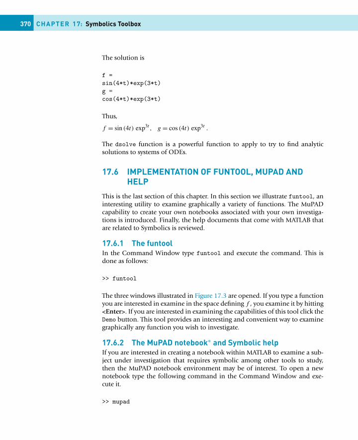
370 CHAPTER 17: Symbolics Toolbox
The solution is
f =sin(4*t)*exp(3*t)g =cos(4*t)*exp(3*t)
Thus,
f = sin (4t) exp3t , g = cos (4t) exp3t .
The dsolve function is a powerful function to apply to try to find analyticsolutions to systems of ODEs.
17.6 IMPLEMENTATION OF FUNTOOL, MUPAD ANDHELP
This is the last section of this chapter. In this section we illustrate funtool, aninteresting utility to examine graphically a variety of functions. The MuPADcapability to create your own notebooks associated with your own investiga-tions is introduced. Finally, the help documents that come with MATLAB thatare related to Symbolics is reviewed.
17.6.1 The funtoolIn the Command Window type funtool and execute the command. This isdone as follows:
>> funtool
The three windows illustrated in Figure 17.3 are opened. If you type a functionyou are interested in examine in the space defining f , you examine it by hitting<Enter>. If you are interested in examining the capabilities of this tool click theDemo button. This tool provides an interesting and convenient way to examinegraphically any function you wish to investigate.
17.6.2 The MuPAD notebook∗ and Symbolic helpIf you are interested in creating a notebook within MATLAB to examine a sub-ject under investigation that requires symbolic among other tools to study,then the MuPAD notebook environment may be of interest. To open a newnotebook type the following command in the Command Window and exe-cute it.
>> mupad
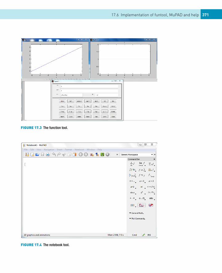
17.6 Implementation of funtool, MuPAD and help 371
FIGURE 17.3 The function tool.
FIGURE 17.4 The notebook tool.
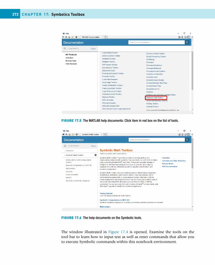
372 CHAPTER 17: Symbolics Toolbox
FIGURE 17.5 The MATLAB help documents: Click item in red box on the list of tools.
FIGURE 17.6 The help documents on the Symbolic tools.
The window illustrated in Figure 17.4 is opened. Examine the tools on thetool bar to learn how to input text as well as enter commands that allow youto execute Symbolic commands within this notebook environment.
17.6 Exercises 373
Finally, to get help on using mupad and other features of the Symbolic toolsclick the circled question mark, ‘?’, just below the word “Help” on the toptool bar. This opened the help window illustrated in Figure 17.5. To get tothe Symbolics help click on Symbolic Math Toolbox in the contents palette.The information in the right hand pane will change to the information in Fig-ure 17.6. Note that there are examples, help for MuPAD and demos that arequite useful.
EXERCISES17.1 Find the derivatives of cosx, and x2 exp2x .17.2 Integrate the function y = 3x2 from x = 0 to x = 10.
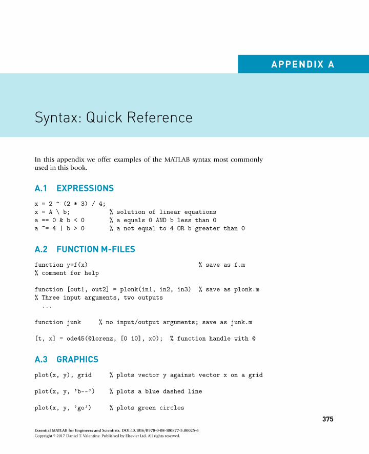
APPENDIX A
Syntax: Quick Reference
In this appendix we offer examples of the MATLAB syntax most commonlyused in this book.
A.1 EXPRESSIONS
x = 2 ^ (2 * 3) / 4;x = A \ b; % solution of linear equationsa == 0 & b < 0 % a equals 0 AND b less than 0a ~= 4 | b > 0 % a not equal to 4 OR b greater than 0
A.2 FUNCTION M-FILES
function y=f(x) % save as f.m% comment for help
function [out1, out2] = plonk(in1, in2, in3) % save as plonk.m% Three input arguments, two outputs
...
function junk % no input/output arguments; save as junk.m
[t, x] = ode45(@lorenz, [0 10], x0); % function handle with @
A.3 GRAPHICS
plot(x, y), grid % plots vector y against vector x on a grid
plot(x, y, ’b--’) % plots a blue dashed line
plot(x, y, ’go’) % plots green circles
375Essential MATLAB for Engineers and Scientists. DOI:10.1016/B978-0-08-100877-5.00025-6Copyright © 2017 Daniel T. Valentine. Published by Elsevier Ltd. All rights reserved.

376 APPENDIX A: Syntax: Quick Reference
plot(y) % if y is a vector plots elements against row numbers% if y is a matrix, plots columns against row numbers
plot(x1, y1, x2, y2) % plots y1 against x1 andy2 against x2 on same graph
semilogy(x, y) % uses a log10 scale for y
polar(theta, r) % generates a polar plot
A.4 if AND switch
if conditionstatement % executed if condition true
end;
if conditionstatement1 % executed if condition true
elsestatement2 % executed if condition false
end;
if a == 0 % test for equalityx = -c / b;
elsex = -b / (2*a);
end;
if condition1 % jumps off ladder at first true conditionstatement1
elseif condition2 % elseif one word!statement2
elseif condition3statement3
...else
statementEend;if condition statement1, else statement2, end % command line
switch lower(expr) % expr is string or scalarcase {’linear’,’bilinear’}
disp(’Method is linear’)case ’cubic’
disp(’Method is cubic’)
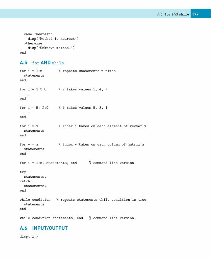
A.5 for and while 377
case ’nearest’disp(’Method is nearest’)
otherwisedisp(’Unknown method.’)
end
A.5 for AND while
for i = 1:n % repeats statements n timesstatements
end;
for i = 1:3:8 % i takes values 1, 4, 7...
end;
for i = 5:-2:0 % i takes values 5, 3, 1...
end;
for i = v % index i takes on each element of vector vstatements
end;
for v = a % index v takes on each column of matrix astatements
end;
for i = 1:n, statements, end % command line version
try,statements,
catch,statements,
end
while condition % repeats statements while condition is truestatements
end;
while condition statements, end % command line version
A.6 INPUT/OUTPUT
disp( x )
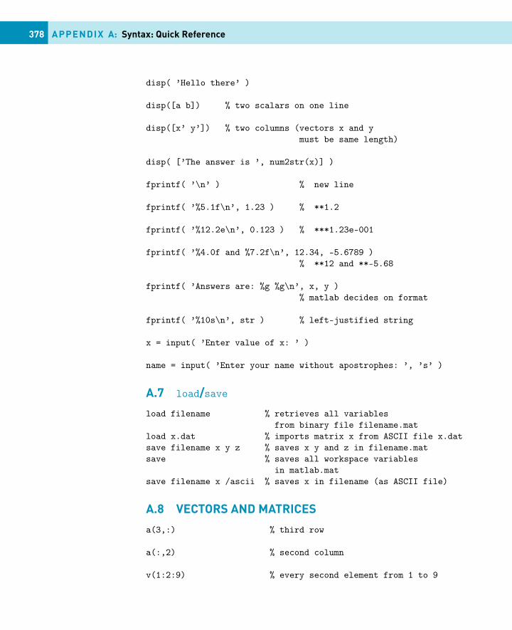
378 APPENDIX A: Syntax: Quick Reference
disp( ’Hello there’ )
disp([a b]) % two scalars on one line
disp([x’ y’]) % two columns (vectors x and ymust be same length)
disp( [’The answer is ’, num2str(x)] )
fprintf( ’\n’ ) % new line
fprintf( ’%5.1f\n’, 1.23 ) % **1.2
fprintf( ’%12.2e\n’, 0.123 ) % ***1.23e-001
fprintf( ’%4.0f and %7.2f\n’, 12.34, -5.6789 )% **12 and **-5.68
fprintf( ’Answers are: %g %g\n’, x, y )% matlab decides on format
fprintf( ’%10s\n’, str ) % left-justified string
x = input( ’Enter value of x: ’ )
name = input( ’Enter your name without apostrophes: ’, ’s’ )
A.7 load/save
load filename % retrieves all variablesfrom binary file filename.mat
load x.dat % imports matrix x from ASCII file x.datsave filename x y z % saves x y and z in filename.matsave % saves all workspace variables
in matlab.matsave filename x /ascii % saves x in filename (as ASCII file)
A.8 VECTORS AND MATRICES
a(3,:) % third row
a(:,2) % second column
v(1:2:9) % every second element from 1 to 9
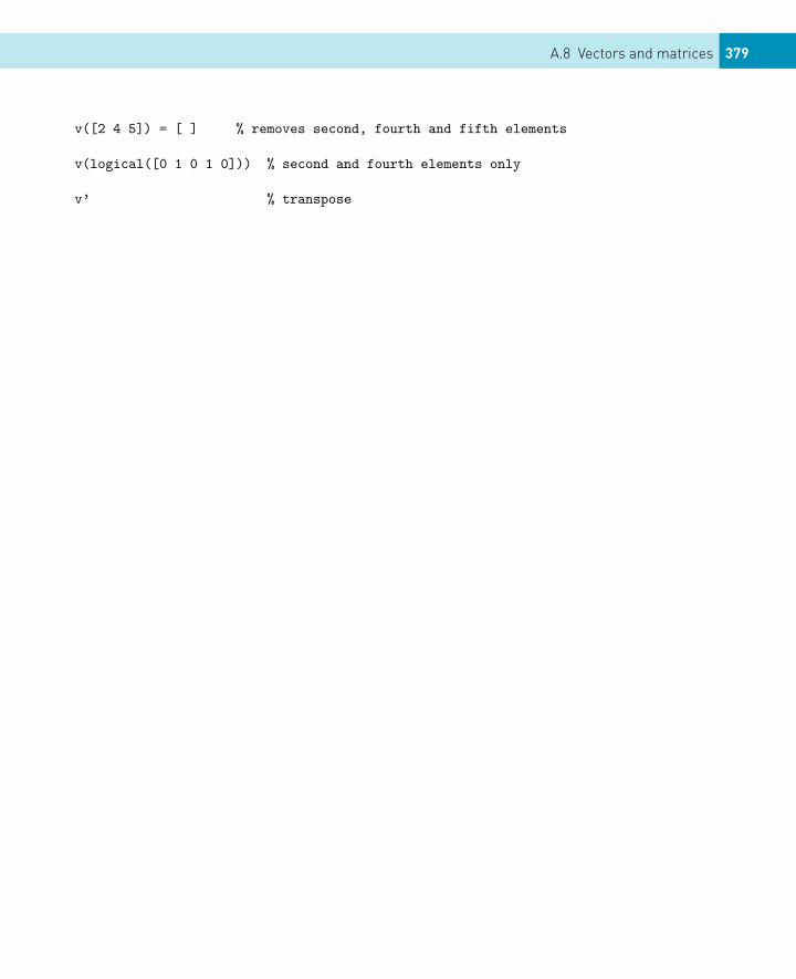
A.8 Vectors and matrices 379
v([2 4 5]) = [ ] % removes second, fourth and fifth elements
v(logical([0 1 0 1 0])) % second and fourth elements only
v’ % transpose
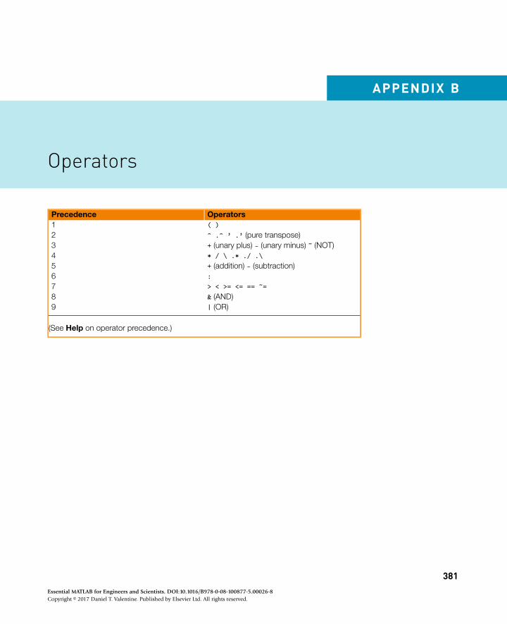
APPENDIX B
Operators
Precedence Operators1 ( )2 ^ .^ ’ .’ (pure transpose)3 + (unary plus) - (unary minus) ~ (NOT)4 * / \ .* ./ .\5 + (addition) - (subtraction)6 :7 > < >= <= == ~=8 & (AND)9 | (OR)
(See Help on operator precedence.)
381Essential MATLAB for Engineers and Scientists. DOI:10.1016/B978-0-08-100877-5.00026-8Copyright © 2017 Daniel T. Valentine. Published by Elsevier Ltd. All rights reserved.
APPENDIX C
Command and Function: Quick Reference
This appendix lists most of the MATLAB commands and functions used in thetext, along with a few others. For a complete list by category (with links todetailed descriptions) see MATLAB: Reference: MATLAB Function Reference:Functions by Category in the online documentation.
The command help by itself displays a list of all the function categories (eachin its own directory).
C.1 GENERAL-PURPOSE COMMANDS
demo Run demoshelp Online helphelpwin Display categories of functions with links to each categorylookfor Keyword search through help entriestype List M-fileswhat Directory listing of M- and MAT-fileswhich Locate functions and files
C.1.1 Managing variables and the workspace
clear Clear variables and functions from memorydisp Display matrix or textlength Length of vectorload Retrieve variables from disksave Save workspace variables to disksize Array dimensionswho, whos List variables in workspace
C.1.2 Files and the operating system
beep Produce beep soundcd Change current working directory
383Essential MATLAB for Engineers and Scientists. DOI:10.1016/B978-0-08-100877-5.00027-XCopyright © 2017 Daniel T. Valentine. Published by Elsevier Ltd. All rights reserved.
384 APPENDIX C: Command and Function: Quick Reference
delete Delete filediary Save text of MATLAB sessiondir Directory listingedit Edit M-file! Execute operating system command
C.1.3 Controlling the Command Window
clc Clear Command Windowecho Echo commands in scriptformat Set output format for disphome Send cursor homemore Control paged output
C.1.4 Starting and quitting MATLAB
exit Terminate MATLABquit Terminate MATLABstartup Execute M-file when MATLAB starts
C.2 LOGICAL FUNCTIONS
all True if all elements of vector are true (nonzero)any True if any element of vector is trueexist Check if variable or file existsfind Find indices of nonzero elementsis* Detect various stateslogical Convert numeric values to logical values
C.3 MATLAB PROGRAMMING TOOLS
error Display error messageeval Interpret string containing MATLAB expressionfeval Function evaluationfor Repeat statement specific number of timesglobal Define global variableif Conditionally execute statementspersistent Define persistent variableswitch Switch among several casestry Begin try blockwhile Repeat statements conditionally
C.4 Matrices 385
C.3.1 Interactive inputinput Prompt user for inputkeyboard Invoke keyboard as script filemenu Generate menu of choices for user inputpause Wait for user response
C.4 MATRICES
eye Identity matrixlinspace Vector with linearly spaced elementsones Matrix of onesrand Uniformly distributed random numbers and arraysrandn Normally distributed random numbers and arrayszeros Matrix of zeros: (colon) Vector with regularly spaced elements
C.4.1 Special variables and constantsans Most recent answereps Floating-point relative accuracyi or j
√−1Inf InfinityNaN Not-a-Numbernargin, nargout Number of actual function argumentspi 3.14159 26535 897 . . .
realmax Largest positive floating-point numberrealmin Smallest positive floating-point numbervarargin, varargout Pass or return variable numbers of arguments
C.4.2 Time and datecalendar Calendarclock Wall clock (complete date and time)date Actual dateetime Elapsed timetic, toc Stopwatchweekday Day of week
C.4.3 Matrix manipulationcat Concatenate arraysdiag Create or extract diagonalfliplr Flip in left/right directionflipud Flip in up/down directionrepmat Replicate and tile array
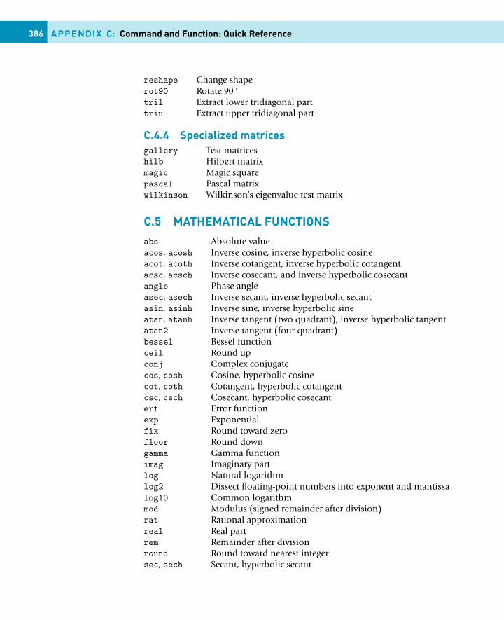
386 APPENDIX C: Command and Function: Quick Reference
reshape Change shaperot90 Rotate 90◦tril Extract lower tridiagonal parttriu Extract upper tridiagonal part
C.4.4 Specialized matricesgallery Test matriceshilb Hilbert matrixmagic Magic squarepascal Pascal matrixwilkinson Wilkinson’s eigenvalue test matrix
C.5 MATHEMATICAL FUNCTIONS
abs Absolute valueacos, acosh Inverse cosine, inverse hyperbolic cosineacot, acoth Inverse cotangent, inverse hyperbolic cotangentacsc, acsch Inverse cosecant, and inverse hyperbolic cosecantangle Phase angleasec, asech Inverse secant, inverse hyperbolic secantasin, asinh Inverse sine, inverse hyperbolic sineatan, atanh Inverse tangent (two quadrant), inverse hyperbolic tangentatan2 Inverse tangent (four quadrant)bessel Bessel functionceil Round upconj Complex conjugatecos, cosh Cosine, hyperbolic cosinecot, coth Cotangent, hyperbolic cotangentcsc, csch Cosecant, hyperbolic cosecanterf Error functionexp Exponentialfix Round toward zerofloor Round downgamma Gamma functionimag Imaginary partlog Natural logarithmlog2 Dissect floating-point numbers into exponent and mantissalog10 Common logarithmmod Modulus (signed remainder after division)rat Rational approximationreal Real partrem Remainder after divisionround Round toward nearest integersec, sech Secant, hyperbolic secant
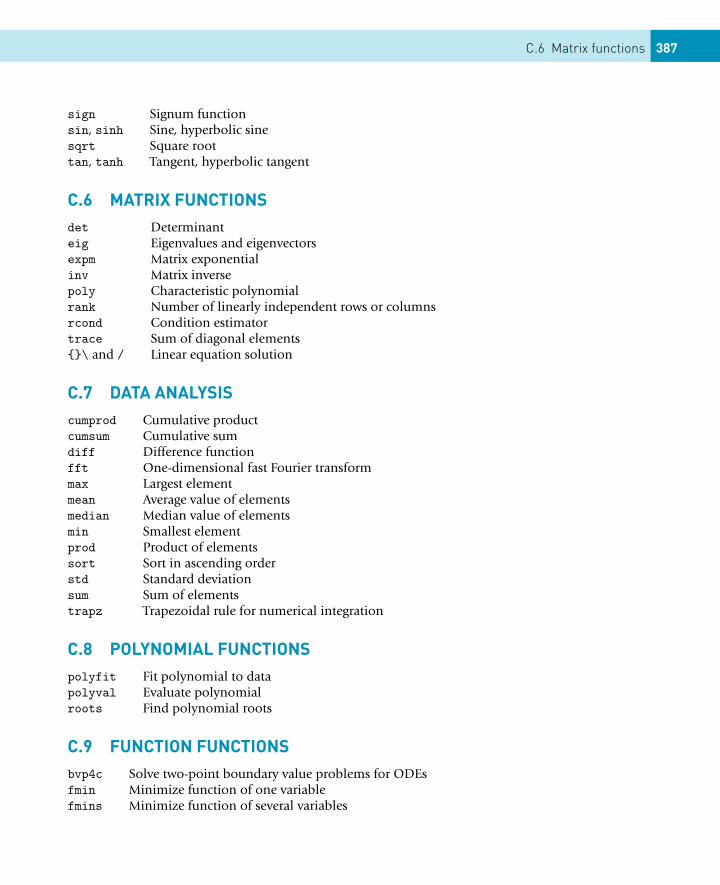
C.6 Matrix functions 387
sign Signum functionsin, sinh Sine, hyperbolic sinesqrt Square roottan, tanh Tangent, hyperbolic tangent
C.6 MATRIX FUNCTIONSdet Determinanteig Eigenvalues and eigenvectorsexpm Matrix exponentialinv Matrix inversepoly Characteristic polynomialrank Number of linearly independent rows or columnsrcond Condition estimatortrace Sum of diagonal elements{}\ and / Linear equation solution
C.7 DATA ANALYSIScumprod Cumulative productcumsum Cumulative sumdiff Difference functionfft One-dimensional fast Fourier transformmax Largest elementmean Average value of elementsmedian Median value of elementsmin Smallest elementprod Product of elementssort Sort in ascending orderstd Standard deviationsum Sum of elementstrapz Trapezoidal rule for numerical integration
C.8 POLYNOMIAL FUNCTIONSpolyfit Fit polynomial to datapolyval Evaluate polynomialroots Find polynomial roots
C.9 FUNCTION FUNCTIONSbvp4c Solve two-point boundary value problems for ODEsfmin Minimize function of one variablefmins Minimize function of several variables
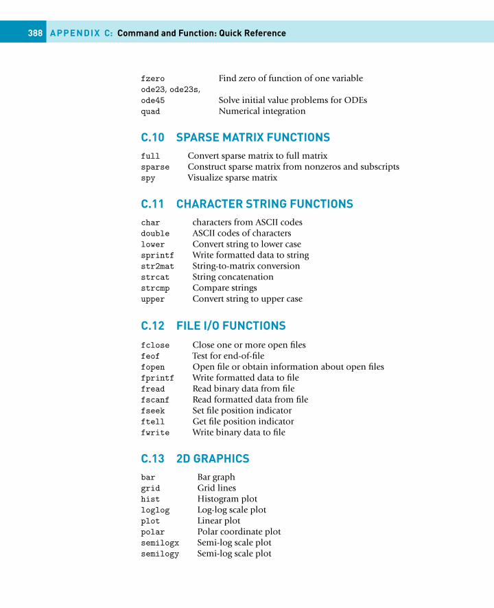
388 APPENDIX C: Command and Function: Quick Reference
fzero Find zero of function of one variableode23, ode23s,ode45 Solve initial value problems for ODEsquad Numerical integration
C.10 SPARSE MATRIX FUNCTIONSfull Convert sparse matrix to full matrixsparse Construct sparse matrix from nonzeros and subscriptsspy Visualize sparse matrix
C.11 CHARACTER STRING FUNCTIONSchar characters from ASCII codesdouble ASCII codes of characterslower Convert string to lower casesprintf Write formatted data to stringstr2mat String-to-matrix conversionstrcat String concatenationstrcmp Compare stringsupper Convert string to upper case
C.12 FILE I/O FUNCTIONS
fclose Close one or more open filesfeof Test for end-of-filefopen Open file or obtain information about open filesfprintf Write formatted data to filefread Read binary data from filefscanf Read formatted data from filefseek Set file position indicatorftell Get file position indicatorfwrite Write binary data to file
C.13 2D GRAPHICSbar Bar graphgrid Grid lineshist Histogram plotloglog Log-log scale plotplot Linear plotpolar Polar coordinate plotsemilogx Semi-log scale plotsemilogy Semi-log scale plot
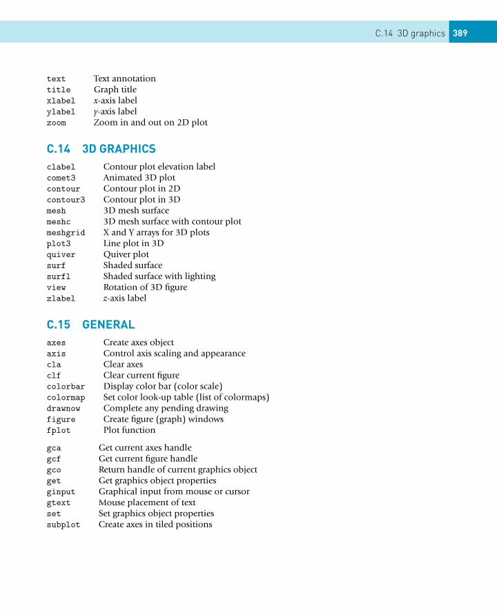
C.14 3D graphics 389
text Text annotationtitle Graph titlexlabel x-axis labelylabel y-axis labelzoom Zoom in and out on 2D plot
C.14 3D GRAPHICSclabel Contour plot elevation labelcomet3 Animated 3D plotcontour Contour plot in 2Dcontour3 Contour plot in 3Dmesh 3D mesh surfacemeshc 3D mesh surface with contour plotmeshgrid X and Y arrays for 3D plotsplot3 Line plot in 3Dquiver Quiver plotsurf Shaded surfacesurfl Shaded surface with lightingview Rotation of 3D figurezlabel z-axis label
C.15 GENERALaxes Create axes objectaxis Control axis scaling and appearancecla Clear axesclf Clear current figurecolorbar Display color bar (color scale)colormap Set color look-up table (list of colormaps)drawnow Complete any pending drawingfigure Create figure (graph) windowsfplot Plot function
gca Get current axes handlegcf Get current figure handlegco Return handle of current graphics objectget Get graphics object propertiesginput Graphical input from mouse or cursorgtext Mouse placement of textset Set graphics object propertiessubplot Create axes in tiled positions
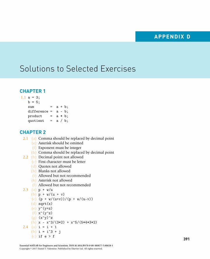
APPENDIX D
Solutions to Selected Exercises
CHAPTER 11.1 a = 3;
b = 5;sum = a + b;difference = a - b;product = a * b;quotient = a / b;
CHAPTER 22.1 (a) Comma should be replaced by decimal point
(e) Asterisk should be omitted(f) Exponent must be integer
(h) Comma should be replaced by decimal point2.2 (b) Decimal point not allowed
(c) First character must be letter(d) Quotes not allowed(h) Blanks not allowed(i) Allowed but not recommended(k) Asterisk not allowed(l) Allowed but not recommended
2.3 (a) p + w/u(b) p + w/(u + v)(c) (p + w/(u+v))/(p + w/(u-v))(d) sqrt(x)(e) y^(y+z)(f) x^(y^z)(g) (x^y)^z(h) x - x^3/(3*2) + x^5/(5*4*3*2)
2.4 (a) i = i + 1(b) i = iˆ3 + j(c) if e > f
391Essential MATLAB for Engineers and Scientists. DOI:10.1016/B978-0-08-100877-5.00028-1Copyright © 2017 Daniel T. Valentine. Published by Elsevier Ltd. All rights reserved.
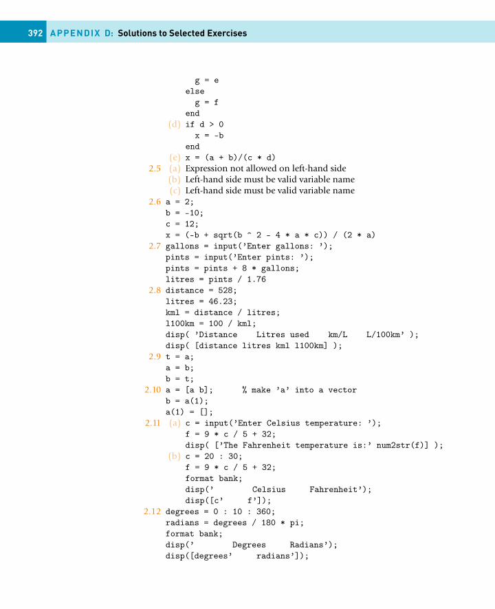
392 APPENDIX D: Solutions to Selected Exercises
g = eelse
g = fend
(d) if d > 0x = -b
end(e) x = (a + b)/(c * d)
2.5 (a) Expression not allowed on left-hand side(b) Left-hand side must be valid variable name(c) Left-hand side must be valid variable name
2.6 a = 2;b = -10;c = 12;x = (-b + sqrt(b ^ 2 - 4 * a * c)) / (2 * a)
2.7 gallons = input(’Enter gallons: ’);pints = input(’Enter pints: ’);pints = pints + 8 * gallons;litres = pints / 1.76
2.8 distance = 528;litres = 46.23;kml = distance / litres;l100km = 100 / kml;disp( ’Distance Litres used km/L L/100km’ );disp( [distance litres kml l100km] );
2.9 t = a;a = b;b = t;
2.10 a = [a b]; % make ’a’ into a vectorb = a(1);a(1) = [];
2.11 (a) c = input(’Enter Celsius temperature: ’);f = 9 * c / 5 + 32;disp( [’The Fahrenheit temperature is:’ num2str(f)] );
(b) c = 20 : 30;f = 9 * c / 5 + 32;format bank;disp(’ Celsius Fahrenheit’);disp([c’ f’]);
2.12 degrees = 0 : 10 : 360;radians = degrees / 180 * pi;format bank;disp(’ Degrees Radians’);disp([degrees’ radians’]);
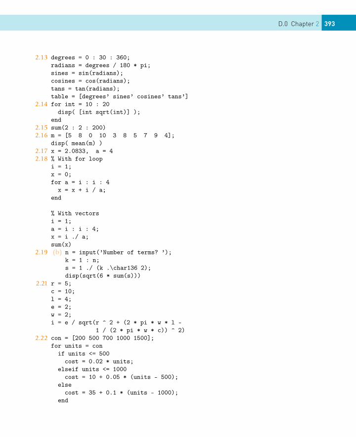
D.0 Chapter 2 393
2.13 degrees = 0 : 30 : 360;radians = degrees / 180 * pi;sines = sin(radians);cosines = cos(radians);tans = tan(radians);table = [degrees’ sines’ cosines’ tans’]
2.14 for int = 10 : 20disp( [int sqrt(int)] );
end2.15 sum(2 : 2 : 200)2.16 m = [5 8 0 10 3 8 5 7 9 4];
disp( mean(m) )2.17 x = 2.0833, a = 42.18 % With for loop
i = 1;x = 0;for a = i : i : 4
x = x + i / a;end
% With vectorsi = 1;a = i : i : 4;x = i ./ a;sum(x)
2.19 (b) n = input(’Number of terms? ’);k = 1 : n;s = 1 ./ (k .\char136 2);disp(sqrt(6 * sum(s)))
2.21 r = 5;c = 10;l = 4;e = 2;w = 2;i = e / sqrt(r ^ 2 + (2 * pi * w * l -
1 / (2 * pi * w * c)) ^ 2)2.22 con = [200 500 700 1000 1500];
for units = conif units <= 500
cost = 0.02 * units;elseif units <= 1000
cost = 10 + 0.05 * (units - 500);else
cost = 35 + 0.1 * (units - 1000);end
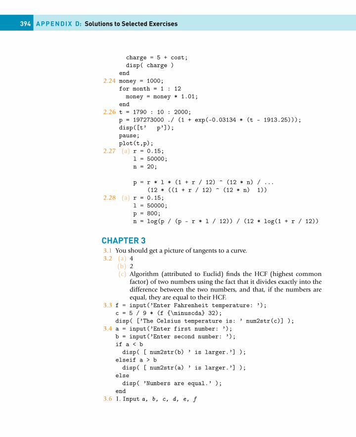
394 APPENDIX D: Solutions to Selected Exercises
charge = 5 + cost;disp( charge )
end2.24 money = 1000;
for month = 1 : 12money = money * 1.01;
end2.26 t = 1790 : 10 : 2000;
p = 197273000 ./ (1 + exp(-0.03134 * (t - 1913.25)));disp([t’ p’]);pause;plot(t,p);
2.27 (a) r = 0.15;l = 50000;n = 20;
p = r * l * (1 + r / 12) ^ (12 * n) / ...(12 * ((1 + r / 12) ^ (12 * n) 1))
2.28 (a) r = 0.15;l = 50000;p = 800;n = log(p / (p - r * l / 12)) / (12 * log(1 + r / 12))
CHAPTER 33.1 You should get a picture of tangents to a curve.3.2 (a) 4
(b) 2(c) Algorithm (attributed to Euclid) finds the HCF (highest common
factor) of two numbers using the fact that it divides exactly into thedifference between the two numbers, and that, if the numbers areequal, they are equal to their HCF.
3.3 f = input(’Enter Fahrenheit temperature: ’);c = 5 / 9 * (f {\minuscda} 32);disp( [’The Celsius temperature is: ’ num2str(c)] );
3.4 a = input(’Enter first number: ’);b = input(’Enter second number: ’);if a < b
disp( [ num2str(b) ’ is larger.’] );elseif a > b
disp( [ num2str(a) ’ is larger.’] );else
disp( ’Numbers are equal.’ );end
3.6 1. Input a, b, c, d, e, f
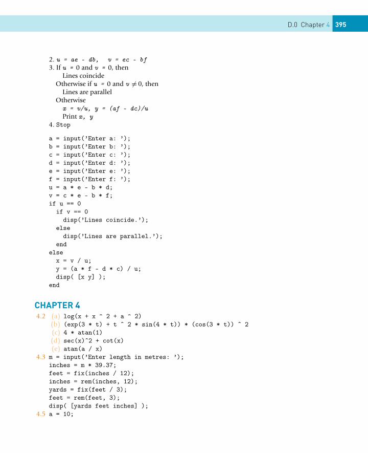
D.0 Chapter 4 395
2. u = ae - db, v = ec - bf3. If u = 0 and v = 0, then
Lines coincideOtherwise if u = 0 and v �= 0, then
Lines are parallelOtherwisex = v/u, y = (af - dc)/uPrint x, y
4. Stop
a = input(’Enter a: ’);b = input(’Enter b: ’);c = input(’Enter c: ’);d = input(’Enter d: ’);e = input(’Enter e: ’);f = input(’Enter f: ’);u = a * e - b * d;v = c * e - b * f;if u == 0
if v == 0disp(’Lines coincide.’);
elsedisp(’Lines are parallel.’);
endelse
x = v / u;y = (a * f - d * c) / u;disp( [x y] );
end
CHAPTER 44.2 (a) log(x + x ^ 2 + a ^ 2)
(b) (exp(3 * t) + t ˆ 2 * sin(4 * t)) * (cos(3 * t)) ˆ 2(c) 4 * atan(1)(d) sec(x)ˆ2 + cot(x)(e) atan(a / x)
4.3 m = input(’Enter length in metres: ’);inches = m * 39.37;feet = fix(inches / 12);inches = rem(inches, 12);yards = fix(feet / 3);feet = rem(feet, 3);disp( [yards feet inches] );
4.5 a = 10;
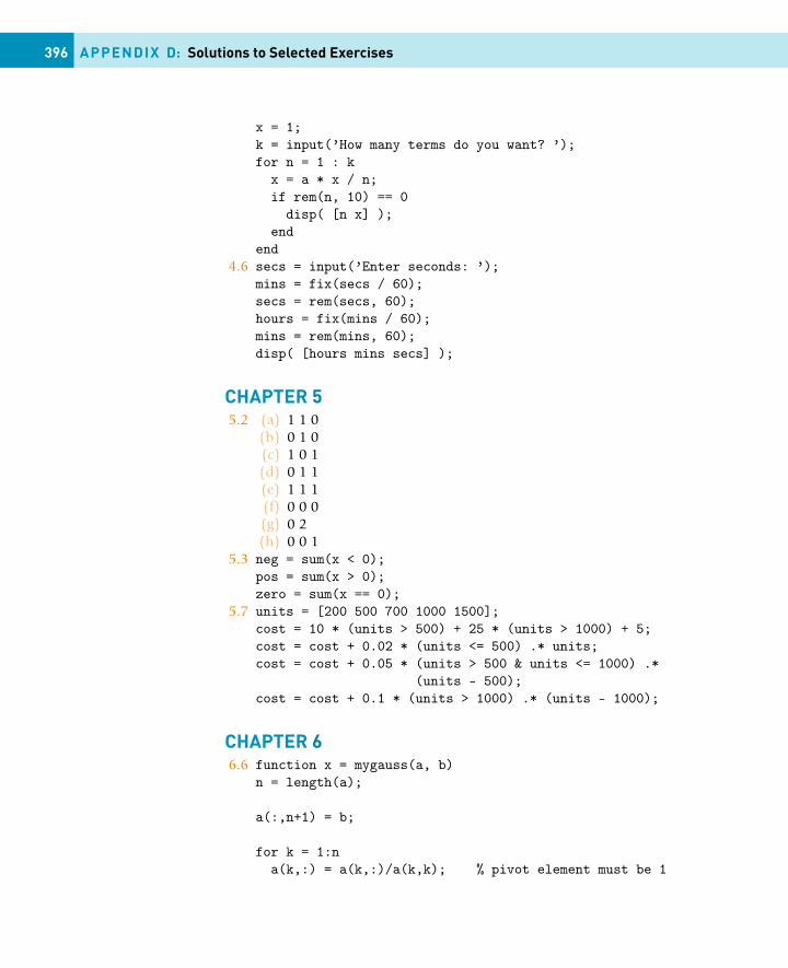
396 APPENDIX D: Solutions to Selected Exercises
x = 1;k = input(’How many terms do you want? ’);for n = 1 : k
x = a * x / n;if rem(n, 10) == 0
disp( [n x] );end
end4.6 secs = input(’Enter seconds: ’);
mins = fix(secs / 60);secs = rem(secs, 60);hours = fix(mins / 60);mins = rem(mins, 60);disp( [hours mins secs] );
CHAPTER 55.2 (a) 1 1 0
(b) 0 1 0(c) 1 0 1(d) 0 1 1(e) 1 1 1(f) 0 0 0(g) 0 2(h) 0 0 1
5.3 neg = sum(x < 0);pos = sum(x > 0);zero = sum(x == 0);
5.7 units = [200 500 700 1000 1500];cost = 10 * (units > 500) + 25 * (units > 1000) + 5;cost = cost + 0.02 * (units <= 500) .* units;cost = cost + 0.05 * (units > 500 & units <= 1000) .*
(units - 500);cost = cost + 0.1 * (units > 1000) .* (units - 1000);
CHAPTER 66.6 function x = mygauss(a, b)
n = length(a);
a(:,n+1) = b;
for k = 1:na(k,:) = a(k,:)/a(k,k); % pivot element must be 1
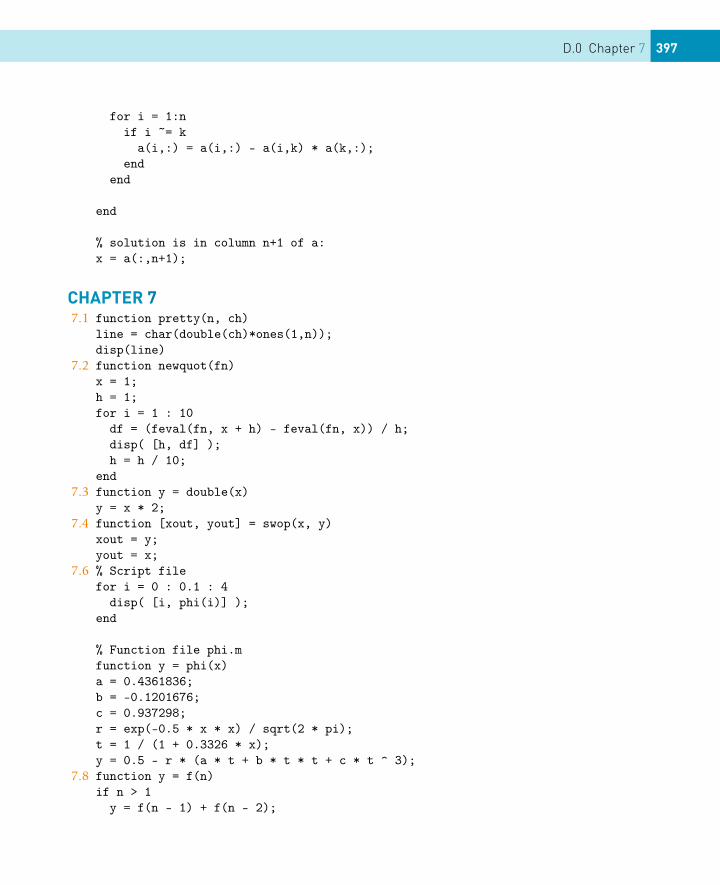
D.0 Chapter 7 397
for i = 1:nif i ~= k
a(i,:) = a(i,:) - a(i,k) * a(k,:);end
end
end
% solution is in column n+1 of a:x = a(:,n+1);
CHAPTER 77.1 function pretty(n, ch)
line = char(double(ch)*ones(1,n));disp(line)
7.2 function newquot(fn)x = 1;h = 1;for i = 1 : 10
df = (feval(fn, x + h) - feval(fn, x)) / h;disp( [h, df] );h = h / 10;
end7.3 function y = double(x)
y = x * 2;7.4 function [xout, yout] = swop(x, y)
xout = y;yout = x;
7.6 % Script filefor i = 0 : 0.1 : 4
disp( [i, phi(i)] );end
% Function file phi.mfunction y = phi(x)a = 0.4361836;b = -0.1201676;c = 0.937298;r = exp(-0.5 * x * x) / sqrt(2 * pi);t = 1 / (1 + 0.3326 * x);y = 0.5 - r * (a * t + b * t * t + c * t ^ 3);
7.8 function y = f(n)if n > 1
y = f(n - 1) + f(n - 2);
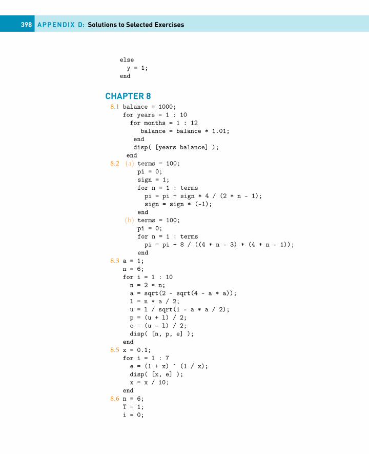
398 APPENDIX D: Solutions to Selected Exercises
elsey = 1;
end
CHAPTER 88.1 balance = 1000;
for years = 1 : 10for months = 1 : 12
balance = balance * 1.01;enddisp( [years balance] );
end8.2 (a) terms = 100;
pi = 0;sign = 1;for n = 1 : terms
pi = pi + sign * 4 / (2 * n - 1);sign = sign * (-1);
end(b) terms = 100;
pi = 0;for n = 1 : terms
pi = pi + 8 / ((4 * n - 3) * (4 * n - 1));end
8.3 a = 1;n = 6;for i = 1 : 10
n = 2 * n;a = sqrt(2 - sqrt(4 - a * a));l = n * a / 2;u = l / sqrt(1 - a * a / 2);p = (u + l) / 2;e = (u - l) / 2;disp( [n, p, e] );
end8.5 x = 0.1;
for i = 1 : 7e = (1 + x) ^ (1 / x);disp( [x, e] );x = x / 10;
end8.6 n = 6;
T = 1;i = 0;
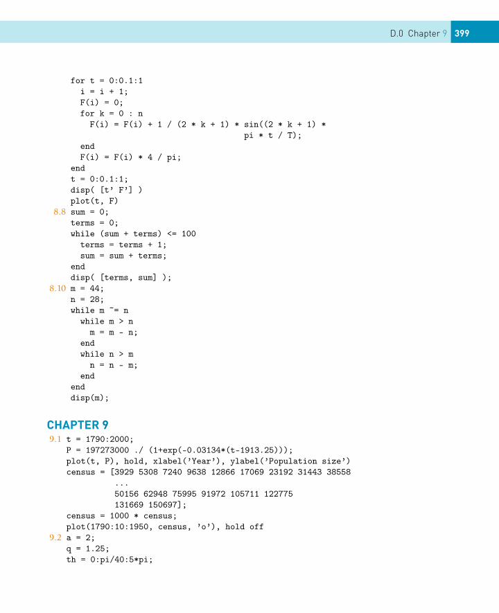
D.0 Chapter 9 399
for t = 0:0.1:1i = i + 1;F(i) = 0;for k = 0 : n
F(i) = F(i) + 1 / (2 * k + 1) * sin((2 * k + 1) *pi * t / T);
endF(i) = F(i) * 4 / pi;
endt = 0:0.1:1;disp( [t’ F’] )plot(t, F)
8.8 sum = 0;terms = 0;while (sum + terms) <= 100
terms = terms + 1;sum = sum + terms;
enddisp( [terms, sum] );
8.10 m = 44;n = 28;while m ~= n
while m > nm = m - n;
endwhile n > m
n = n - m;end
enddisp(m);
CHAPTER 99.1 t = 1790:2000;
P = 197273000 ./ (1+exp(-0.03134*(t-1913.25)));plot(t, P), hold, xlabel(’Year’), ylabel(’Population size’)census = [3929 5308 7240 9638 12866 17069 23192 31443 38558
...50156 62948 75995 91972 105711 122775131669 150697];
census = 1000 * census;plot(1790:10:1950, census, ’o’), hold off
9.2 a = 2;q = 1.25;th = 0:pi/40:5*pi;
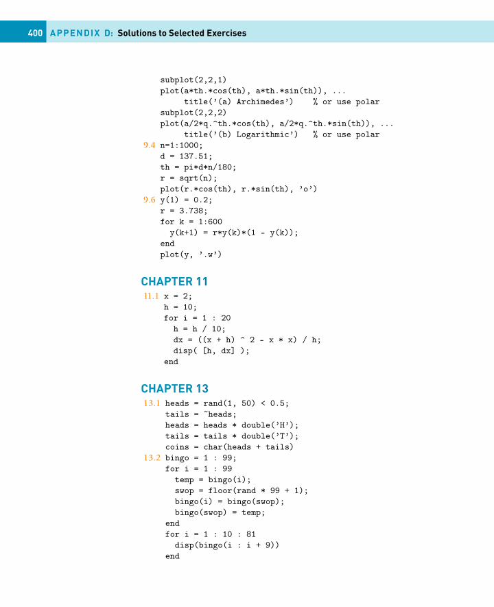
400 APPENDIX D: Solutions to Selected Exercises
subplot(2,2,1)plot(a*th.*cos(th), a*th.*sin(th)), ...
title(’(a) Archimedes’) % or use polarsubplot(2,2,2)plot(a/2*q.^th.*cos(th), a/2*q.^th.*sin(th)), ...
title(’(b) Logarithmic’) % or use polar9.4 n=1:1000;
d = 137.51;th = pi*d*n/180;r = sqrt(n);plot(r.*cos(th), r.*sin(th), ’o’)
9.6 y(1) = 0.2;r = 3.738;for k = 1:600
y(k+1) = r*y(k)*(1 - y(k));endplot(y, ’.w’)
CHAPTER 1111.1 x = 2;
h = 10;for i = 1 : 20
h = h / 10;dx = ((x + h) ^ 2 - x * x) / h;disp( [h, dx] );
end
CHAPTER 1313.1 heads = rand(1, 50) < 0.5;
tails = ~heads;heads = heads * double(’H’);tails = tails * double(’T’);coins = char(heads + tails)
13.2 bingo = 1 : 99;for i = 1 : 99
temp = bingo(i);swop = floor(rand * 99 + 1);bingo(i) = bingo(swop);bingo(swop) = temp;
endfor i = 1 : 10 : 81
disp(bingo(i : i + 9))end
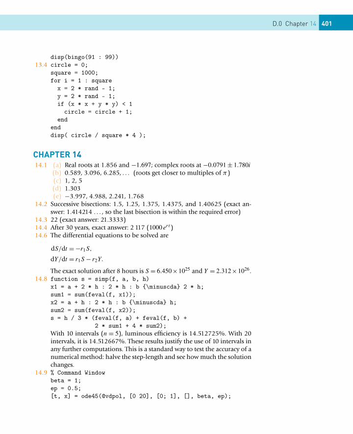
D.0 Chapter 14 401
disp(bingo(91 : 99))13.4 circle = 0;
square = 1000;for i = 1 : square
x = 2 * rand - 1;y = 2 * rand - 1;if (x * x + y * y) < 1
circle = circle + 1;end
enddisp( circle / square * 4 );
CHAPTER 1414.1 (a) Real roots at 1.856 and −1.697; complex roots at −0.0791 ± 1.780i
(b) 0.589, 3.096, 6.285, . . . (roots get closer to multiples of π)(c) 1, 2, 5(d) 1.303(e) −3.997, 4.988, 2.241, 1.768
14.2 Successive bisections: 1.5, 1.25, 1.375, 1.4375, and 1.40625 (exact an-swer: 1.414214 . . . , so the last bisection is within the required error)
14.3 22 (exact answer: 21.3333)14.4 After 30 years, exact answer: 2 117 (1000 ert )14.6 The differential equations to be solved are
dS/dt = −r1S,
dY/dt = r1S − r2Y.
The exact solution after 8 hours is S = 6.450×1025 and Y = 2.312×1026.14.8 function s = simp(f, a, b, h)
x1 = a + 2 * h : 2 * h : b {\minuscda} 2 * h;sum1 = sum(feval(f, x1));x2 = a + h : 2 * h : b {\minuscda} h;sum2 = sum(feval(f, x2));s = h / 3 * (feval(f, a) + feval(f, b) +
2 * sum1 + 4 * sum2);With 10 intervals (n = 5), luminous efficiency is 14.512725%. With 20intervals, it is 14.512667%. These results justify the use of 10 intervals inany further computations. This is a standard way to test the accuracy of anumerical method: halve the step-length and see how much the solutionchanges.
14.9 % Command Windowbeta = 1;ep = 0.5;[t, x] = ode45(@vdpol, [0 20], [0; 1], [], beta, ep);
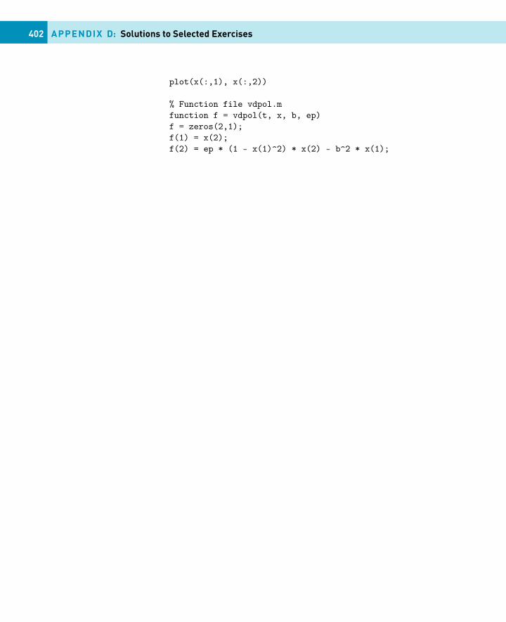
402 APPENDIX D: Solutions to Selected Exercises
plot(x(:,1), x(:,2))
% Function file vdpol.mfunction f = vdpol(t, x, b, ep)f = zeros(2,1);f(1) = x(2);f(2) = ep * (1 - x(1)^2) * x(2) - b^2 * x(1);
Index
Symbols\, 46, 153%, 43@
function handle creation, 171&, 114’, 116, 130.’, 116.*, 48./, 48.\, 48.ˆ, 48:, 9, 130;, 7, 50˜, 114|, 114π , 8π̃ , 192
estimation of, 2923-D plot, 206
Aabs, 73, 100acos, 100acosh, 100air resistance, 269algebra, 356algorithm, 84all, 119, 137
example, 120AND, 114angle, 73animation, 222comet3, 207
ans, 35, 49
any, 119example, 120
apostrophe, 130argument
input, 93input, pass by reference, 169input, pass by value, 169
arithmetic operator, 46array, 9, 34
2-D, 127cell, 249multi-dimensional, 142
Array Editor, 35array operation, 48, 138asin, 100asinh, 100aspect ratio, 73assignment, 7assignment statement, 50atan, 100atan2, 73, 100atanh, 100axis, 200
equal, 73normal, 73
axis limits, 200azimuth, 213
Bbacteria division, 286bacteria growth, 292, 305balance delimiters, 53bar graph, 243base workspace, 167best fit, 155binomial coefficient, 181
404 Index
Bisection method, 297bit, 35bitwise logical operations, 115break, 184, 190breakpoint, 175Bubble Sort, 244bug, 255byte, 35
Ccalculus, 356calendar, 8camel caps, 34cantilever beam, 263cartesian co-ordinates, 204case, 72case sensitivity, 34ceil, 100cell, 249, 250cell array, 249celldisp, 252cellplot, 252chaos, 223, 233, 310
butterfly, 312trajectory, 312
cla, 203clc, 8clear, 35clear M-file, 168clf, 203clipboard, 26clock, 62, 101colon operator, 9, 37, 130colon operator, initialization, 37colon operator, precedence, 47color, 200colorbar, 226colormap, 225comet3, 207command, 50command line, 7command line editing, 7Command Window, 5command/function duality, 173comment, 43compiler, 29complex conjugate transpose, 73complex numbers, 72
condition estimator, 156conj, 73Contents.m, 167context menu, 29continuation of statement, 43, 50continue, 190contour, 210contour plot, 23contour3, 210cos, 101cosh, 101cot, 101Crank-Nicolson method, 315csc, 101cumsum, 101current directory, 28curve fitting, 320cut and paste, 26
Ddata types, 45date, 8, 101deal, 249Debugger, 174debugging, 255degrees to radians, 8del2, 227delimiter highlighting, 53demo, 12determinate repetition, 181diag, 138diary, 41dice, 114diff, 303differential equation, 304, 356differentiation, 356disp, 54display
scale factor, 57division
matrix, 156dot product, 48dot-transpose operator, 116double, 45double precision, 45doubling time of an investment, 185drawnow, 223
Eediting a plot, 220
Index 405
eig, 146eigenvalue, 148eigenvector, 149electrical circuit, 264element-by-element operation, 48ellipse, equation of, 232ellipsis, 43, 50elseif, 68empty, 37empty array, 120end, 132eps, 111error
fatal, 255logical, 256rounding, 257run-time, 174syntax, 255
etime, 62Euler’s method, 304exclusive OR, 115exist, 119exp, 101explicit list, initializing vectors, 36expm, 146, 308exponent, 45exponential
matrix, 308exponential fit, 155exponential growth, 305exporting ASCII data
save, 104exporting binary data
save, 105expression, 44, 46, 49
ans, 49display suppressed, 49logical, 65, 114
eye, 135
Ffactorial, 59false, 109fast Fourier transform, 325feval, 171Fibonacci numbers, 180field, 247fieldnames, 248
figure, 9, 203figure window, 10, 202find, 119findobj, 218finite difference scheme, 307, 314fix, 101fixed point, 45, 55fliplr, 138flipud, 138floating-point, 45, 55floor, 60, 101for, 60
command line version, 61index, 60iteration count, 60more general, 61most general form, 139nested, 140, 184replaced by vectorization, 62used for determinate loop, 191
format, 55, 56formula
vectorization, 52Fourier series, 193, 325fplot, 205fractal, 233free fall problem, 264frequency distribution, 243full, 160full matrix, 158function, 50, 166
handle for passing as argument, 171help, 166MATLAB Function Reference, 100name resolution, 174P-code file, 170private, 170subfunction, 170
function functions, 173function M-file, 163function/command duality, 173fzero, 299
GGauss reduction, 162Gaussian random number, 291gca, 215gcf, 215
406 Index
gco, 215get, 216Gibbs phenomenon, 194ginput, 203global, 167gradient, 211, 212graph, 9
easy-to-use commands, 198graphics
2-D, 1973-D, 2063-D rotation, 213axis limits, 200contour plot, 209cropping a surface, 211editing, 220editing a plot, 220line type, 200logarithmic plot, 203mesh surface, 207multiple plots, 199, 202plotting symbol, 200polar co-ordinates, 204rapidly changing functions, 205saving, 229vector field, 211
grid, 199gtext, 199, 242guessing game, 184
HH1 line, 166Halley’s comet, 233handle
function, 171graphics object, 214
Handle Graphics objects, 214Harmonic analysis, 325help
for a function, 166Help Navigator, 99helpwin, 99hexadecimal, 56hidden name, 174, 256histogram, 243hold, 199
Ii, 72
identity matrix, 135if, 65
command line version, 64elseif, 68nested, 70vectorized with logical vector, 121
if-else, 67command line, 67
ill conditioning, 156, 161imag, 73importing ASCII data
load, 105importing binary data
load, 106inclusive OR, 115indeterminate repetition, 181, 184index of for, 60Inf, 7infinity, 7initialization, colon operator, 37initialization, explicit list, 36inline object, 92input argument, 93integration, 356interpolation, 301interpreter, 29inv, 146isempty, 120isglobal, 167isinf, 120isnan, 120isothermal, 210iteration count, 60
Jj, 72
KKnuth, 188
Lleast squares, 155left division, 46, 153, 156Legendre polynomial, 180length, 102Leslie matrix, 147lighting, 228limit of sequence, 59line numbers, 174line style, 200
Index 407
linear equationsover-determined, 154residual, 154solution, 152under-determined, 155
linspace, 38list
sorting, 244load, 105, 106LODE, 308log, 102log10, 102logarithmic plot, 203logarithmic spiral, 231logical error, 256logical expression, 64, 65, 109, 114
vector, 110logical function, 119logical operator, 68, 114
precedence, 115logical vector, 110
subscripting with, 118loglog, 204logspace, 38lookfor, 166loop
determinate, 181indeterminate, 184
Lorenz, 310Lotka-Volterra model, 313lu, 146
MM-file, 28
function, 163function passed as argument, 171
magic square, 23, 137mantissa, 45, 56marker, 200Markov chain, 150MATLAB functions, 92matrix, 36, 40, 127
array operation, 138creating, 129deleting rows and columns, 134duplicating rows and columns, 133enlarging, 130full, 158
Leslie, 147multiplication, 143plot, 197sparse, 158subscript, 129transpose, 40, 130visualization, 212
matrix division, 156matrix exponential, 308matrix exponentiation, 145matrix multiplication, 143matrix operation, 143matrix operations, 48max, 102, 246mean, 102mechanical system, 337menu, 190mesh, 208mesh surface, 207meshc, 210meshgrid, 207Mexican hat, 23min, 102, 246mlock, 168Monte Carlo estimation of π , 292more, 55, 188multi-dimensional array, 142multiple lines in Command Window, 27multiple plots, 202multiple plots on same axes, 199munlock, 168
Nname hiding, 174, 256NaN, 7nargin, 170nargout, 170nested for, 140nested fors, 184nested ifs, 70Newton quotient, 179, 258, 302Newton’s method, 58, 163Newton’s method in general, 295normally distributed random number,
291NOT, 114not-a-number, 7
408 Index
num2str, 55number, 45numerical differentiation, 302numerical integration, 300numerical method, 295
Bisection method, 297differential equation, 304differentiation, 302Euler’s method, 304integration, 300Newton quotient, 302Newton’s method, 295partial differential equation, 314predictor-corrector, 307Runge-Kutta method, 309Simpson’s rule, 301solution of equations, 295Trapezoidal rule, 300
numerical solution of differentialequations, 304
numerical solution of equations, 295
Oobject, 252
Handle Graphics, 214object-oriented programming, 252ones, 135operand, 46operation
array, 48element-by element, 48matrix, 143
operatorarithmetic, 46colon, 130dot-transpose, 116left division, 153logical, 68, 114precedence, 46, 116relational, 65transpose, 116
operator precedence, complete list, 116,181
OR, 114exclusive, 115
oscillator, 337
output, 54paging, 55suppressed with semicolon, 50
output argument, 165over-determined system, 154
PP-code file, 170paging, 188paging output, 55partial differential equation, 314pascal, 136pause, 213pcode, 170persistent variable, 167pi, 8plot, 197
3-D version, 206logarithmic scale, 203polar co-ordinates, 204
plot edit mode, 220plot3, 206plotedit, 220plotyy, 199Poisson process, 288polar, 204polar co-ordinates, 204polynomial fitting, 320pow2, 102pre-allocation, 237precedence, 116
arithmetic operators, 46colon operator, 47logical operator, 115transpose, 47
precedence of operators, complete list,116
predator-prey model, 313predictor-corrector method, 307prime number
largest known, 188test, 187
private function, 170prod, 102Profiler, 171program, 25projectile problem, 264projectile trajectory, 188
Index 409
Property Editor, 206pseudo-code, 41pseudo-random number, 102
Qqr, 146quad, 302quadrature, 302quiver, 211quote in string, 54
Rradio-active decay, 294RAM, 29rand, 102, 113, 135, 283
seeding, 284uniform, 283
randn, 291random access memory, 29random number, 39, 113
generation, 283normal, 291uniform, 283
random numberscounting, 113
random walk, 150, 243, 286rat, 56real, 73realmax, 45, 102realmin, 45, 102recall
smart, 7recursion, 177redimensioning, 238reference, pass by, 169relational operator, 65relative accuracy, 45rem, 102removing element of vector, 119removing elements of an array, 39repmat, 133reshape, 133reshaping a matrix, 132residual, 154right division, 156rmfield, 249rolling a dice, 285rolling dice, 114
root of an equation, 295roots, 299rot90, 138rounding error, 257, 302run-time error, 174Runge-Kutta method, 309
Ssave, 104, 105saving a file, 27saving a graph, 229scalar, 9scalar expansion, 48scalar product, 48scientific notation, 45
display, 56scope, 167script, 28
recommended way to run, 29script file, 28seeding rand, 284semi-colon, 7semilogx, 204semilogy, 203sensitivity analysis, 161separator, 50series for π , 192set, 216Simpson’s rule, 301simulation, 114, 243
bacteria division, 286bacteria growth, 292estimation of π , 292game of eights, 293radio-active decay, 294random walk, 286rolling a dice, 285spinning coins, 284traffic flow, 288
single-precision, 45size, 35smart indenting, 61smart recall, 7sort, 244, 246sort, bubble, 244sound, 183sparse, 158, 159, 316sparse matrix, 158, 316
410 Index
spinning coins, 284spiral
Archimedes, 231logarithmic, 231
spring, mass damper model, 337sprintf, 242spy, 160, 213sqrt, 8stable age distribution, 149statement, 7, 50
assignment, 50continuation, 50
string, 54containing quote, 54
struct, 248structure, 247structure plan, 27, 41subfunction, 170subplot, 202subscript, 39, 129
logical vectors, 118vector, 118
subscript out of range, 130subscripting with logical vectors, 118sunflower head, 232surf, 208surfc, 210svd, 146switch, 71symbolic mathematical, 355syntax error, 255
Ttab completion, 11Taylor series
exponential, 179terminal speed, 270TeX characters, 220text, 199tic, 62tiling, 134title, 199toc, 62top down programming, 42traffic flow, 288transpose, 39, 40, 130
complex conjugate, 73transpose operator, 116
transpose operator, highest precedence,47
Trapezoidal rule, 300tridiagonal matrix, 315trigonometry, 356tril, 138triu, 138true, 109truecolor, 228truncation error, 320type, 28
Uunder-determined system, 155uniformly distributed random number,
283update process, 235
Vvalue, pass by, 169Van der Pol’s equation, 322varargin, 170, 251varargout, 251variable, 7, 29, 33
global, 167persistent, 167scope, 167termed arrays by MATLAB, 34
vector, 9, 36colon operator, 37explicit list, 36incompatible sizes, 256pre-allocation, 237redimensioning, 238removing element, 119scalar product, 48subscript, 39, 118transpose, 39
vectorization, 52instead of for, 62
view, 213visualization of matrix, 212
Wwhile, 185
command line form, 185used for indeterminate loop, 192vector condition, 185
who, 35whos, 35
Index 411
why, 25workspace, 34
base, 167function, 167
Workspace Browser, 35
Xxlabel, 199xor, 115
Yylabel, 199
Zzero of a function, 295zeros, 135zlabel, 207zoom, 321


