A Matlab Program for Analysis of Kinematics

Example of a four-bar linkage mechanism

mm180mm180mm260

mm80

OCBCABOA

0220sin90

0180cos900sin90sin1300cos90cos130

0sin130sin400cos130cos40

0sin400cos40

:equations Constraint

1

33

33

3322

3322

2211

2211

11

11

tyx

yyxxyyxx

yx

A

B

CO

y

x

11

1

22

33

3

2

333222111 ,,,,,,,, unknown 9for equations 9 thesolve To yxyxyxT q2

The Jacobian matrix and the right-side of the velocity equations

000000100cos9010000000sin9001000000

cos9010cos13010000sin9001sin13001000000cos13010cos4010000sin13001sin4001000000cos4010000000sin4001

3

3

32

32

2

2

9

8

7

6

5

4

3

2

1

J

200000000

qβq velocity for the solve To J

3

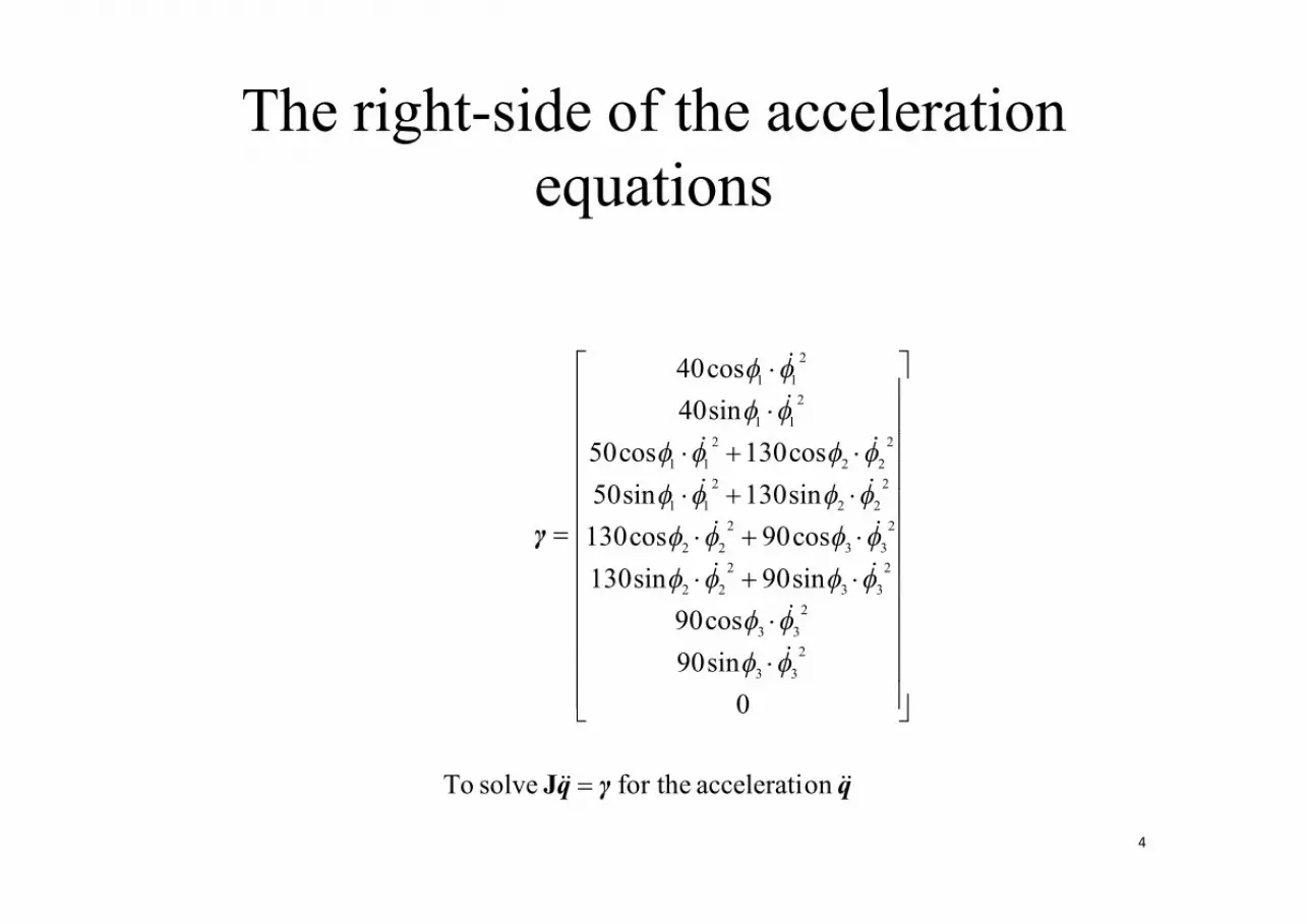
The right-side of the acceleration equations

0sin90cos90

sin90sin130cos90cos130sin130sin50cos130cos50

sin40cos40

233

233

233

222

233

222

222

2

222

2

2

2

γ

qγq onaccelerati for the solve To J

4

The procedure of m-file0at start and Initialize t

tq solve toposition initial hsolver witnonlinear Call

solve to with andmatrix Jacobian Determine tt qqβ

solve to with Determine tt qqγ

iterationnext of position initialnew theasit set and

motion intended with Assume Δtt q

ttt qqq and , of response timePlot the

themanimate and bars theof positions theDetermine5

The code of m.file (1)1. % Set up the time interval and the initial positions of the nine coordinates2. T_Int=0:0.01:2;3. X0=[0 50 pi/2 125.86 132.55 0.2531 215.86 82.55 4.3026];4. global T5. Xinit=X0;6.7. % Do the loop for each time interval8. for Iter=1:length(T_Int);9. T=T_Int(Iter);10. % Determine the displacement at the current time11. [Xtemp,fval] = fsolve(@constrEq4bar,Xinit);12.13. % Determine the velocity at the current time14. phi1=Xtemp(3); phi2=Xtemp(6); phi3=Xtemp(9);15. JacoMatrix=Jaco4bar(phi1,phi2,phi3);16. Beta=[0 0 0 0 0 0 0 0 2*pi]';17. Vtemp=JacoMatrix\Beta;18.19. % Determine the acceleration at the current time20. dphi1=Vtemp(3); dphi2=Vtemp(6); dphi3=Vtemp(9); 21. Gamma=Gamma4bar(phi1,phi2,phi3,dphi1,dphi2,dphi3);22. Atemp=JacoMatrix\Gamma;23.24. % Record the results of each iteration25. X(:,Iter)=Xtemp; V(:,Iter)=Vtemp; A(:,Iter)=Atemp;26.27. % Determine the new initial position to solve the equation of the next28. % iteration and assume that the kinematic motion is with inertia29. if Iter==130. Xinit=X(:,Iter);31. else32. Xinit=X(:,Iter)+(X(:,Iter)-X(:,Iter-1));33. end34.35.end

6

The code of m.file (2)36.% T vs displacement plot for the nine coordinates37.figure38.for i=1:9;39. subplot(9,1,i)40. plot (T_Int,X(i,:))41. set(gca,'xtick',[], 'FontSize', 5)42.end43.% Reset the bottom subplot to have xticks44.set(gca,'xtickMode', 'auto')45.46.% T vs velocity plot for the nine coordinates47.figure48.for i=1:9;49. subplot(9,1,i)50. plot (T_Int,V(i,:))51. set(gca,'xtick',[], 'FontSize', 5)52.end53.set(gca,'xtickMode', 'auto')54.55.% T vs acceleration plot for the nine coordinates56.figure57.for i=1:9;58. subplot(9,1,i)59. plot (T_Int,A(i,:))60. AxeSup=max(A(i,:));61. AxeInf=min(A(i,:));62. if AxeSup-AxeInf<0.0163. axis([-inf,inf,(AxeSup+AxeSup)/2-0.1 (AxeSup+AxeSup)/2+0.1]);64. end65. set(gca,'xtick',[], 'FontSize', 5)66.end67.set(gca,'xtickMode', 'auto') 7

The code of m.file (3)68.% Determine the positions of the four revolute joints at each iteration69.Ox=zeros(1,length(T_Int));70.Oy=zeros(1,length(T_Int));71.Ax=80*cos(X(3,:));72.Ay=80*sin(X(3,:));73.Bx=Ax+260*cos(X(6,:));74.By=Ay+260*sin(X(6,:));75.Cx=180*ones(1,length(T_Int));76.Cy=zeros(1,length(T_Int));77.78.% Animation79.figure80.for t=1:length(T_Int);81. bar1x=[Ox(t) Ax(t)];82. bar1y=[Oy(t) Ay(t)];83. bar2x=[Ax(t) Bx(t)];84. bar2y=[Ay(t) By(t)];85. bar3x=[Bx(t) Cx(t)];86. bar3y=[By(t) Cy(t)];87.88. plot (bar1x,bar1y,bar2x,bar2y,bar3x,bar3y);89. axis([-120,400,-120,200]);90. axis normal91.92. M(:,t)=getframe;93.end

8

Initialization1. % Set up the time interval and the initial positions of the nine coordinates2. T_Int=0:0.01:2;3. X0=[0 50 pi/2 125.86 132.55 0.2531 215.86 82.55 4.3026];4. global T5. Xinit=X0;

1. The sentence is notation that is behind symbol “%”.

2. Simulation time is set from 0 to 2 with Δt = 0.01.

3. Set the appropriate initial positions of the 9 coordinates which are used to solve nonlinear solver.

4. Declare a global variable T which is used to represent the current time t and determine the

driving constraint for angular velocity.

9

Determine the displacement10. [Xtemp,fval] = fsolve(@constrEq4bar,Xinit);

a. function F=constrEq4bar(X)b.c. global Td.e. x1=X(1); y1=X(2); phi1=X(3);f. x2=X(4); y2=X(5); phi2=X(6);g. x3=X(7); y3=X(8); phi3=X(9);h.i. F=[ -x1+40*cos(phi1);j. -y1+40*sin(phi1);k. x1+40*cos(phi1)-x2+130*cos(phi2);l. y1+40*sin(phi1)-y2+130*sin(phi2);m. x2+130*cos(phi2)-x3+90*cos(phi3);n. y2+130*sin(phi2)-y3+90*sin(phi3);o. x3+90*cos(phi3)-180;p. y3+90*sin(phi3);q. phi1-2*pi*T-pi/2];

10. Call the nonlinear solver fsolve in which the constraint equations and initial values are necessary. The

initial values is mentioned in above script. The constraint equations is written as a function (which can

be treated a kind of subroutine in Matlab) as following and named as constrEq4bar. The fsolve finds a

root of a system of nonlinear equations and adopts the trust-region dogleg algorithm by default.

The equation of driving constraint is depended on current time T

10

Determine the velocity14. phi1=Xtemp(3); phi2=Xtemp(6); phi3=Xtemp(9);15. JacoMatrix=Jaco4bar(phi1,phi2,phi3);16. Beta=[0 0 0 0 0 0 0 0 2*pi]';17. Vtemp=JacoMatrix\Beta;

15. Call the function Jaco4bar to obtain the Jacobian Matrix depended on current values of

displacement.

16. Declare the right-side of the velocity equations.

17. Solve linear equation by left matrix division “\” roughly the same as J-1β. The algorithm adopts

several methods such as LAPACK, CHOLMOD, and LU. Please find the detail in Matlab Help.

a. function JacoMatrix=Jaco4bar(phi1,phi2,phi3)b.c. JacoMatrix=[ -1 0 -40*sin(phi1) 0 0 0 0 0 0;d. 0 -1 40*cos(phi1) 0 0 0 0 0 0;e. 1 0 -40*sin(phi1) -1 0 -130*sin(phi2) 0 0 0;f. 0 1 40*cos(phi1) 0 -1 130*cos(phi2) 0 0 0;g. 0 0 0 1 0 -130*sin(phi2) -1 0 -90*sin(phi3);h. 0 0 0 0 1 130*cos(phi2) 0 -1 90*cos(phi3);i. 0 0 0 0 0 0 1 0 -90*sin(phi3);j. 0 0 0 0 0 0 0 1 90*cos(phi3);k. 0 0 1 0 0 0 0 0 0];

11

Determine the acceleration20. dphi1=Vtemp(3); dphi2=Vtemp(6); dphi3=Vtemp(9); 21. Gamma=Gamma4bar(phi1,phi2,phi3,dphi1,dphi2,dphi3);22. Atemp=JacoMatrix\Gamma;

21. Call the function Gamma4bar to obtain the right-side of the velocity equations depended on

current values of velocity.

22. Solve linear equation to obtain the current acceleration.

a. function Gamma=Gamma4bar(phi1,phi2,phi3,dphi1,dphi2,dphi3)b.c. Gamma=[ 40*cos(phi1)*dphi1^2;d. 40*sin(phi1)*dphi1^2;e. 40*cos(phi1)*dphi1^2+130*cos(phi2)*dphi2^2;f. 40*sin(phi1)*dphi1^2+130*sin(phi2)*dphi2^2;g. 130*cos(phi2)*dphi2^2+90*cos(phi3)*dphi3^2;h. 130*sin(phi2)*dphi2^2+90*sin(phi3)*dphi3^2;i. 90*cos(phi3)*dphi3^2;j. 90*sin(phi3)*dphi3^2;k. 0];

12

Determine next initial positions 29. if Iter==130. Xinit=X(:,Iter);31. else32. Xinit=X(:,Iter)+(X(:,Iter)-X(:,Iter-1));33. end

29.~33. Predict the next initial positions with assumption of inertia except the first time of the loop.

13

Plot time response37.figure

38.for i=1:9;

39. subplot(9,1,i)

40. plot (T_Int,X(i,:))

41. set(gca,'xtick',[], 'FontSize', 5)

42.end

43.% Reset the bottom subplot to have xticks

44.set(gca,'xtickMode', 'auto')

45.

46.% T vs velocity plot for the nine coordinates

47.figure

48.for i=1:9;

37.…

37. Create a blank figure .

39. Locate the position of subplot in the figure.

40. Plot the nine subplots for the time responses of nine coordinates.

41. Eliminate x-label for time-axis and set the font size of y-label.

44. Resume x-label at bottom because the nine subplots share the same time-axis.

47.~ It is similar to above.14

Animation69.Ox=zeros(1,length(T_Int));70.Oy=zeros(1,length(T_Int));71.Ax=80*cos(X(3,:));72.Ay=80*sin(X(3,:));73.Bx=Ax+260*cos(X(6,:));

74.…

69. Determine the displacement of revolute joint.

80. Repeat to plot the locations by continue time elapsing.

81. Determine the horizontal location of .

88. Plot .

89. Set an appropriate range of axis.

80.for t=1:length(T_Int);81. bar1x=[Ox(t) Ax(t)];82. bar1y=[Oy(t) Ay(t)];83. bar2x=[Ax(t) Bx(t)];84. bar2y=[Ay(t) By(t)];85. bar3x=[Bx(t) Cx(t)];86. bar3y=[By(t) Cy(t)];87.88. plot (bar1x,bar1y,bar2x,bar2y,bar3x,bar3y);89. axis([-120,400,-120,200]);90. axis normal91.92. M(:,t)=getframe;93.end

OA

OCBCABOA and , , ,15

Time response of displacement

1x

1

1y

2x

2

2y

3x

3

3y

t16

Time response of velocity

1x

1

1y

2x

2

2y

3x

3

3y

t17

Time response of acceleration

1x

1

1y

2x

2

2y

3x

3

3y

t18

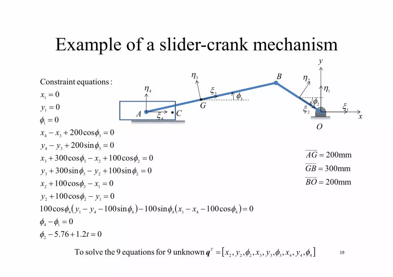
Example of a slider-crank mechanism

mm200mm300mm200

BOGBAG

02.176.50

0cos100sin100sin100cos1000cos1000cos100

0sin100sin3000cos100cos300

0sin2000cos200

000

:equations Constraint

2

14

44144414

122

122

2233

2233

334

334

1

1

1

t

xxyyyyxxyyxx

yyxx

yx

444333222 ,,,,,,,, unknown 9for equations 9 thesolve To yxyxyxT q

A

B

CO

y

x4

4

2

23

33

21

1G

19

The Jacobian matrix and the right-side of the velocity equations

00000036000003500000000340033323100000002928000000272600240000000230220020000191801716000000015014130120000100980000000006504000000000000000300000000000020000000000001

12

11

10

9

8

7

6

5

4

3

2

1

J

2.100000000000

2

3

2

3

3

cos10027 ,17sin30015

sin10023 ,13cos2009sin2005

135 ,24 ,20 ,16 ,12 ,8 ,4136 ,34 ,26 ,22 ,18 ,14 ,10 ,6 ,3 ,2 ,1

144144

4

4

3

sincos10033

29322831

cos10029sin10028

cos30019

yyxx

20

The right-side of the acceleration equations

00

10sin100

cos100

sin100sin300

cos100cos300

sin200

cos200

000

222

222

222

233

222

233

233

233

γ

γ

4144142

444144414 cos100sin100sin200cos20010 where yyxxyyxx

21

Animation

22

Time response of displacement

2x

2

2y

3x

3

3y

4x

4

4y

t23

Time response of velocity

2x

2

2y

3x

3

3y

4x

4

4y

t24

Time response of acceleration

2x

2

2y

3x

3

3y

t

4x

4

4y

25

26

% This script of matlab m.file is used to solve the kinematic problem of a % four-bar linkage for the mechanical dynamics course. % Designer: C. Y. Chuang % Proto-type: 13-July-2012 % Adviser: Prof. Yang clear all clc % Set up the time interval and the initial positions of the nine coordinates T_Int=0:0.01:2; X0=[0 40 pi/2 125.86 132.55 0.2531 215.86 82.55 4.3026]; global T Xinit=X0; % Do the loop for each time interval for Iter=1:length(T_Int); T=T_Int(Iter); % Determine the position at the current time [Xtemp,fval] = fsolve(@constrEq4bar,Xinit); % Determine the velocity at the current time phi1=Xtemp(3); phi2=Xtemp(6); phi3=Xtemp(9); JacoMatrix=Jaco4bar(phi1,phi2,phi3); Beta=[0 0 0 0 0 0 0 0 2*pi]'; Vtemp=JacoMatrix\Beta; % Determine the acceleration at the current time dphi1=Vtemp(3); dphi2=Vtemp(6); dphi3=Vtemp(9); Gamma=Gamma4bar(phi1,phi2,phi3,dphi1,dphi2,dphi3); Atemp=JacoMatrix\Gamma; % Record the results of each iteration X(:,Iter)=Xtemp; V(:,Iter)=Vtemp; A(:,Iter)=Atemp;

Main program: kinematic4bar

27

% Determine the new initial position to solve the equation of the next % iteration and assume that the kinematic motion is with inertia if Iter==1 Xinit=X(:,Iter); else Xinit=X(:,Iter)+(X(:,Iter)-X(:,Iter-1)); end end % T vs displacement plot for the nine coordinates figure for i=1:9; subplot(9,1,i) plot (T_Int,X(i,:),'linewidth',1) AxeSup=max(X(i,:)); AxeInf=min(X(i,:)); AxeSpac=0.05*(AxeSup-AxeInf); if AxeSup-AxeInf<0.01 axis([-inf,inf,(AxeSup+AxeSup)/2-0.1 (AxeSup+AxeSup)/2+0.1]); else axis([-inf,inf,AxeInf-AxeSpac,AxeSup+AxeSpac]); end set(gca,'xtick',[], 'FontSize', 5,'FontName','timesnewroman') end % Reset the bottom subplot to have xticks set(gca,'xtickMode', 'auto') % T vs velocity plot for the nine coordinates figure for i=1:9; subplot(9,1,i) plot (T_Int,V(i,:),'linewidth',1) AxeSup=max(V(i,:)); AxeInf=min(V(i,:)); AxeSpac=0.05*(AxeSup-AxeInf); if AxeSup-AxeInf<0.01 axis([-inf,inf,(AxeSup+AxeSup)/2-0.1 (AxeSup+AxeSup)/2+0.1]); else axis([-inf,inf,AxeInf-AxeSpac,AxeSup+AxeSpac]);

28

end set(gca,'xtick',[], 'FontSize', 5,'FontName','timesnewroman') end set(gca,'xtickMode', 'auto') % T vs acceleration plot for the nine coordinates figure for i=1:9; subplot(9,1,i) plot (T_Int,A(i,:),'linewidth',1) AxeSup=max(A(i,:)); AxeInf=min(A(i,:)); AxeSpac=0.05*(AxeSup-AxeInf); if AxeSup-AxeInf<0.01 axis([-inf,inf,(AxeSup+AxeSup)/2-0.1 (AxeSup+AxeSup)/2+0.1]); else axis([-inf,inf,AxeInf-AxeSpac,AxeSup+AxeSpac]); end set(gca,'xtick',[], 'FontSize', 5,'FontName','timesnewroman') end set(gca,'xtickMode', 'auto') % Determine the positions of the four revolute joints at each iteration Ox=zeros(1,length(T_Int)); Oy=zeros(1,length(T_Int)); Ax=80*cos(X(3,:)); Ay=80*sin(X(3,:)); Bx=Ax+260*cos(X(6,:)); By=Ay+260*sin(X(6,:)); Cx=180*ones(1,length(T_Int)); Cy=zeros(1,length(T_Int)); % Animation figure for t=1:length(T_Int); bar1x=[Ox(t) Ax(t)]; bar1y=[Oy(t) Ay(t)]; bar2x=[Ax(t) Bx(t)]; bar2y=[Ay(t) By(t)]; bar3x=[Bx(t) Cx(t)];

29

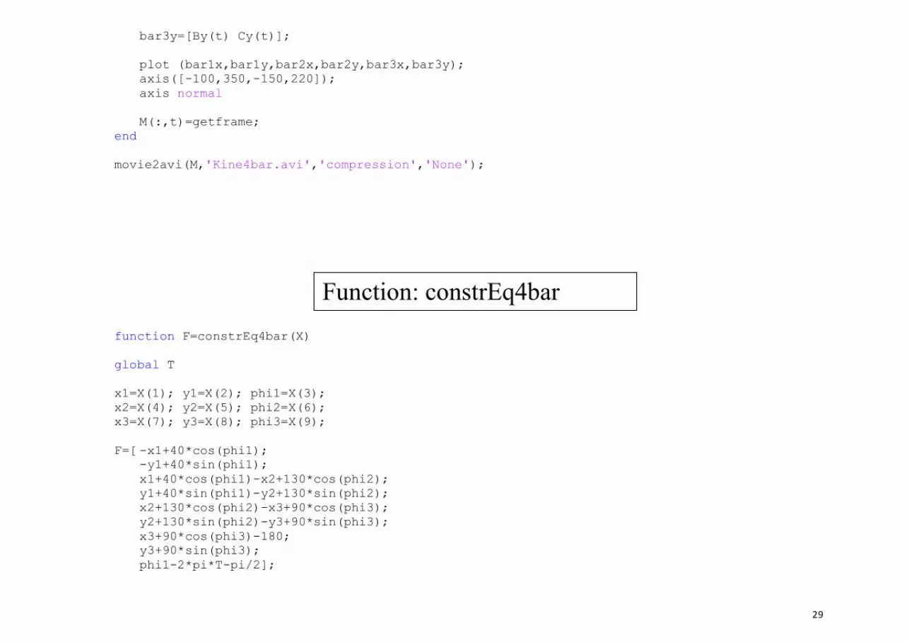
bar3y=[By(t) Cy(t)]; plot (bar1x,bar1y,bar2x,bar2y,bar3x,bar3y); axis([-100,350,-150,220]); axis normal M(:,t)=getframe; end movie2avi(M,'Kine4bar.avi','compression','None'); function F=constrEq4bar(X) global T x1=X(1); y1=X(2); phi1=X(3); x2=X(4); y2=X(5); phi2=X(6); x3=X(7); y3=X(8); phi3=X(9); F=[ -x1+40*cos(phi1); -y1+40*sin(phi1); x1+40*cos(phi1)-x2+130*cos(phi2); y1+40*sin(phi1)-y2+130*sin(phi2); x2+130*cos(phi2)-x3+90*cos(phi3); y2+130*sin(phi2)-y3+90*sin(phi3); x3+90*cos(phi3)-180; y3+90*sin(phi3); phi1-2*pi*T-pi/2];

Function: constrEq4bar

30

function JacoMatrix=Jaco4bar(phi1,phi2,phi3) JacoMatrix=[ -1 0 -40*sin(phi1) 0 0 0 0 0 0; 0 -1 40*cos(phi1) 0 0 0 0 0 0; 1 0 -40*sin(phi1) -1 0 -130*sin(phi2) 0 0 0; 0 1 40*cos(phi1) 0 -1 130*cos(phi2) 0 0 0; 0 0 0 1 0 -130*sin(phi2) -1 0 -90*sin(phi3); 0 0 0 0 1 130*cos(phi2) 0 -1 90*cos(phi3); 0 0 0 0 0 0 1 0 -90*sin(phi3); 0 0 0 0 0 0 0 1 90*cos(phi3); 0 0 1 0 0 0 0 0 0]; function Gamma=Gamma4bar(phi1,phi2,phi3,dphi1,dphi2,dphi3) Gamma=[40*cos(phi1)*dphi1^2; 40*sin(phi1)*dphi1^2; 40*cos(phi1)*dphi1^2+130*cos(phi2)*dphi2^2; 40*sin(phi1)*dphi1^2+130*sin(phi2)*dphi2^2; 130*cos(phi2)*dphi2^2+90*cos(phi3)*dphi3^2; 130*sin(phi2)*dphi2^2+90*sin(phi3)*dphi3^2; 90*cos(phi3)*dphi3^2; 90*sin(phi3)*dphi3^2; 0];

Function: Jaco4bar

Function: Gamma4bar

31

% This script of matlab m.file is used to solve the kinematic problem of a % slider-crank mechanism for the mechanical dynamics course. % Designer: C. Y. Chuang % Proto-type: 13-July-2012 % Adviser: Prof. Yang clear all clc % Set up the time interval and the initial positions of the nine coordinates T_Int=0:0.01:2*pi/1.2; X0=[0 0 0 0 0 5.76 0 0 0 -500 0 0];; global T Xinit=X0; % Do the loop for each time interval for Iter=1:length(T_Int); T=T_Int(Iter); % Determine the position at the current time [Xtemp,fval] = fsolve(@constrEqSC,Xinit); % Determine the velocity at the current time x1=Xtemp(1); y1=Xtemp(2); phi1=Xtemp(3); phi2=Xtemp(6); phi3=Xtemp(9); x4=Xtemp(10); y4=Xtemp(11); phi4=Xtemp(12); JacoMatrix=JacoSC(x1,y1,phi1, phi2, phi3,x4,y4,phi4); Beta=[ 0 0 0 0 0 0 0 0 0 0 0 1.2]'; Vtemp=JacoMatrix\Beta; % Determine the acceleration at the current time dx1=Vtemp(1); dy1=Vtemp(2); dphi1=Vtemp(3); dphi2=Vtemp(6); dphi3=Vtemp(9); dx4=Vtemp(10); dy4=Vtemp(11); dphi4=Vtemp(12); Gamma=GammaSC(x1,y1,phi2,phi3,x4,y4,phi4,dx1,dy1,dphi2,dphi3,dx4,dy4,dphi4);

Main program: kinematicSC

32

Atemp=JacoMatrix\Gamma; % Record the results of each iteration X(:,Iter)=Xtemp; V(:,Iter)=Vtemp; A(:,Iter)=Atemp; % Determine the new initial position to solve the equation of the next % iteration and assume that the kinematic motion is with inertia if Iter==1 Xinit=X(:,Iter); else Xinit=X(:,Iter)+(X(:,Iter)-X(:,Iter-1)); end end % T vs displacement plot for the nine coordinates figure for i=1:9; subplot(9,1,i) plot (T_Int,X(i+3,:),'linewidth',1) AxeSup=max(X(i+3,:)); AxeInf=min(X(i+3,:)); AxeSpac=0.05*(AxeSup-AxeInf); if AxeSup-AxeInf<0.01 axis([-inf,inf,(AxeSup+AxeSup)/2-0.1 (AxeSup+AxeSup)/2+0.1]); else axis([-inf,inf,AxeInf-AxeSpac,AxeSup+AxeSpac]); end set(gca,'xtick',[], 'FontSize', 5,'FontName','timesnewroman') end % Reset the bottom subplot to have xticks set(gca,'xtickMode', 'auto') % T vs velocity plot for the nine coordinates figure for i=1:9; subplot(9,1,i) plot (T_Int,V(i+3,:),'linewidth',1) AxeSup=max(V(i+3,:)); AxeInf=min(V(i+3,:));

33

AxeSpac=0.05*(AxeSup-AxeInf); if AxeSup-AxeInf<0.01 axis([-inf,inf,(AxeSup+AxeSup)/2-0.1 (AxeSup+AxeSup)/2+0.1]); else axis([-inf,inf,AxeInf-AxeSpac,AxeSup+AxeSpac]); end set(gca,'xtick',[], 'FontSize', 5,'FontName','timesnewroman') end set(gca,'xtickMode', 'auto') % T vs acceleration plot for the nine coordinates figure for i=1:9; subplot(9,1,i) plot (T_Int,A(i+3,:),'linewidth',1) AxeSup=max(A(i+3,:)); AxeInf=min(A(i+3,:)); AxeSpac=0.05*(AxeSup-AxeInf); if AxeSup-AxeInf<0.01 axis([-inf,inf,(AxeSup+AxeSup)/2-0.1 (AxeSup+AxeSup)/2+0.1]); else axis([-inf,inf,AxeInf-AxeSpac,AxeSup+AxeSpac]); end set(gca,'xtick',[], 'FontSize', 5,'FontName','timesnewroman') end set(gca,'xtickMode', 'auto') % Determine the positions of the four revolute joints at each iteration Ox=zeros(1,length(T_Int)); Oy=zeros(1,length(T_Int)); Bx=-200*cos(X(6,:)); By=-200*sin(X(6,:)); Ax=Bx-500*cos(X(9,:)); Ay=By-500*sin(X(9,:)); % Animation figure for t=1:length(T_Int); bar2x=[Ox(t) Bx(t)]; bar2y=[Oy(t) By(t)];

34

bar3x=[Bx(t) Ax(t)]; bar3y=[By(t) Ay(t)]; blockx=[Ax(t)-100 Ax(t)+100 Ax(t)+100 Ax(t)-100 Ax(t)-100]; blocky=[Ay(t)-20 Ay(t)-20 Ay(t)+20 Ay(t)+20 Ay(t)-20]; plot (bar2x,bar2y,bar3x,bar3y,blockx,blocky); axis([-900,300,-500,500]); axis normal M(:,t)=getframe; end movie2avi(M,'KineSC.avi','compression','None'); function F=constrEqSC(X) global T x1=X(1); y1=X(2); phi1=X(3); x2=X(4); y2=X(5); phi2=X(6); x3=X(7); y3=X(8); phi3=X(9); x4=X(10); y4=X(11); phi4=X(12); F=[ x1; y1; phi1; x4-x3+200*cos(phi3); y4-y3+200*sin(phi3); x3+300*cos(phi3)-x2+100*cos(phi2); y3+300*sin(phi3)-y2+100*sin(phi2); x2+100*cos(phi2)-x1; y2+100*sin(phi2)-y1; (100*cos(phi4))*(y1-y4-100*sin(phi4))-(100*sin(phi4))*(x1-x4-100*cos(phi4)) phi4-phi1; phi2-5.76+1.2*T];

Function: constrEqSC

35

function JacoMatrix=JacoSC(x1,y1,phi1, phi2, phi3,x4,y4,phi4) % The variable E means the element which is a vector of nonzero values in % the sparse matrix JacoMatrix. E([1 2 3 6 10 14 18 22 26 34 36])=1; E([4 8 12 16 20 24 35])=-1; E(5)=-200*sin(phi3); E(9)=200*cos(phi3); E([13 23])=-100*sin(phi2); E(15)=-300*sin(phi3); E([17 27])=100*cos(phi2); E(19)=300*cos(phi3); E(28)=-100*sin(phi4); E(29)=100*cos(phi4); E(31)=-E(28); E(32)=-E(29); E(33)=-100*( cos(phi4)*(x1-x4) +cos(phi4)*(y1-y4) ); JacoMatrix=[ E(1) 0 0 0 0 0 0 0 0 0 0 0; 0 E(2) 0 0 0 0 0 0 0 0 0 0; 0 0 E(3) 0 0 0 0 0 0 0 0 0; 0 0 0 0 0 0 E(4) 0 E(5) E(6) 0 0; 0 0 0 0 0 0 0 E(8) E(9) E(10) 0 0; 0 0 0 E(12) 0 E(13) E(14) 0 E(15) 0 0 0; 0 0 0 0 E(16) E(17) 0 E(18) E(19) 0 0 0; E(20) 0 0 E(22) 0 E(23) 0 0 0 0 0 0; 0 E(24) 0 0 E(26) E(27) 0 0 0 0 0 0; E(28) E(29) 0 0 0 0 0 0 0 E(31) E(32) E(33); 0 0 E(34) 0 0 0 0 0 0 0 0 E(35); 0 0 0 0 0 E(36) 0 0 0 0 0 0];

Function: JacoSC

36

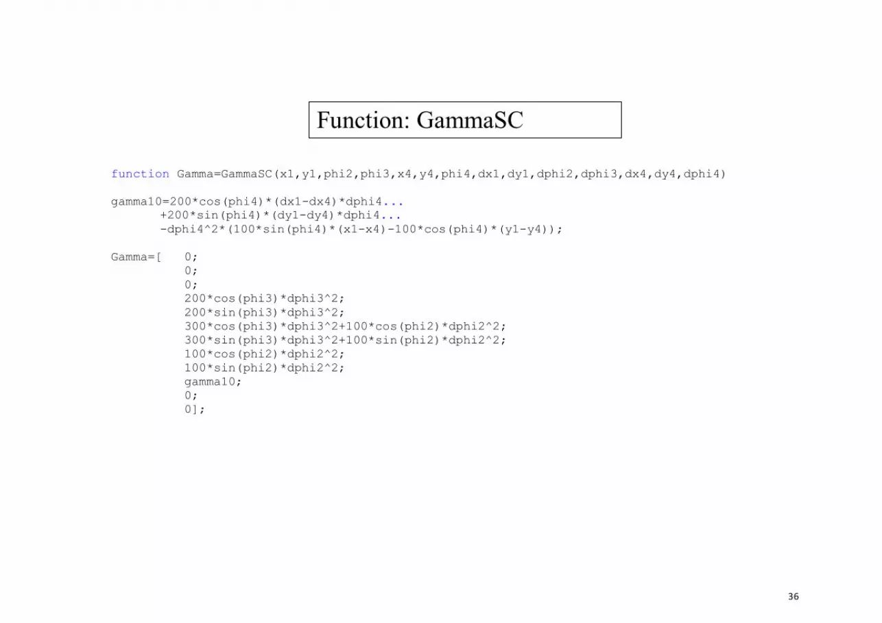
function Gamma=GammaSC(x1,y1,phi2,phi3,x4,y4,phi4,dx1,dy1,dphi2,dphi3,dx4,dy4,dphi4) gamma10=200*cos(phi4)*(dx1-dx4)*dphi4... +200*sin(phi4)*(dy1-dy4)*dphi4... -dphi4^2*(100*sin(phi4)*(x1-x4)-100*cos(phi4)*(y1-y4)); Gamma=[ 0; 0; 0; 200*cos(phi3)*dphi3^2; 200*sin(phi3)*dphi3^2; 300*cos(phi3)*dphi3^2+100*cos(phi2)*dphi2^2; 300*sin(phi3)*dphi3^2+100*sin(phi2)*dphi2^2; 100*cos(phi2)*dphi2^2; 100*sin(phi2)*dphi2^2; gamma10; 0; 0];

Function: GammaSC