1281

Estimating animal behavior and residency from movement data

M. W. Pedersen, T. A. Patterson, U. H. Thygesen and H. Madsen

M. W. Pedersen (mwp@imm.dtu.dk) and H. Madsen, Dept for Informatics and Mathematical Modelling, Technical Univ. of Denmark, DK-2800 Kgs. Lyngby, Denmark. – T. A. Patterson, Commonwealth Scientific and Industrial Research Organization (CSIRO), Wealth From Oceans Flagship and Marine and Atmospheric Research, GPO Box 1538, Hobart, Tasmania 7001, Australia. – U. H. Thygesen, Natl Inst. of Aquatic Resources, Technical Univ. of Denmark, DK-2920 Charlottenlund, Denmark.

We present a process-based approach to estimate residency and behavior from uncertain and temporally correlated move-ment data collected with electronic tags. The estimation problem is formulated as a hidden Markov model (HMM) on a spatial grid in continuous time, which allows straightforward implementation of barriers to movement. Using the grid to explicitly resolve space, location estimation can be supplemented by or based entirely on environmental data (e.g. tem-perature, daylight). The HMM method can therefore analyze any type of electronic tag data. The HMM computes the joint posterior probability distribution of location and behavior at each point in time. With this, the behavioral state of the animal can be associated to regions in space, thus revealing migration corridors and residence areas. We demonstrate the inferential potential of the method by analyzing satellite-linked archival tag data from a southern bluefin tuna Thunnus maccoyii where longitudinal coordinates inferred from daylight are supplemented by latitudinal information in recorded sea surface temperatures.

Movements of individual animals constitute important and highly complex processes which influence the outcome of many large-scale ecological processes. For many species, individual movements can now be assessed empirically using electronic tracking and logging techniques (Cooke et al. 2004). Such information is increasing our understanding of both individual species and ecosystems. However, several problems invariably arise in the resulting data which require a statistical solution. Namely, the need to correct for location uncertainty (Vincent et al. 2002), handle missing or irregu-lar data (Johnson et al. 2008) and the incorporation of bar-riers to movement (Ovaskainen 2004).

The most immediate problem facing empirical measure-ment of movement is noise in the observations of location. The noise is mainly a result of two factors: uncertainty inher-ent in the observation process, and the fact that observa-tions are a discrete sub-sample of the underlying continuous movement process. This error structure necessitates statisti-cal models that are able to separate the two noise contri-butions to estimate the most likely location of an animal at any point in time. State-space models (SSMs, Patterson et al. 2008b) have recently become the favored tool for this (Jonsen et al. 2006, Pedersen et al. 2008, Patterson et al. 2010). As an alternative to SSMs Sumner et al. (2009) sug-gests a Bayesian approach which merges an unconventional underlying movement model with a likelihood model for the observed data.

Recently, models have been investigated which incor-porate different movement modes reflecting shifts in the

underlying behavioral state of the animal (Morales et al. 2004). Behavioral states, being unobserved, are often vaguely defined. Commonly the labels attached to each state reflect predictions from optimal foraging theory. Thus, animals should search more intensively in productive habi-tats and minimize time in other areas. The labels used for the different behavior states include ‘migrating’, ‘ballistic’, or ‘extensive’ for fast, directed movements and ‘diffusive’, ‘foraging’ or ‘intensive’ for slow movements with many direction changes and increased probability of foraging. Such behaviors driving movement are typically hidden to the observer and may only be inferred from the movement data itself (Patterson et al. 2009).

Data from tracking technology is often non-spatial (e.g. data from a temperature logger) yet can be mobilized in a spatial context. As demonstrated below, data from a tem-perature sensor can be used to inform about spatial location if synoptic spatial coverage of similar data is available. Fortu-nately, spatial data (e.g. remote sensing data) is often avail-able, and can provide exactly this. Such data have been used by Nielsen et al. (2006) to improve location estimates from an SSM.

Animal movements are often constrained by barriers or edges. For example, the sea is a barrier to terrestrial animals, as is land for aquatic animals. Such restrictions provide use-ful information in that certain movement trajectories can be ruled out. This is an aspect which has not been included in many SSMs, in particular those that rely on linear-Gaussian models which cannot incorporate hard constraints.

Oikos 120: 1281–1290, 2011 doi: 10.1111/j.1600-0706.2011.19044.x

© 2011 The Authors. Oikos © 2011 Nordic Society OikosSubject Editor: Justin Travis. Accepted 11 January 2011

1282

With Monte Carlo simulation methods (Sumner et al. 2009) it is possible to implement barriers using rejection sampling, however this has a tendency to bias the location distribu-tion near barriers because naively proposed movement paths encountering barriers are removed. Methods using reflec-tive barriers (Pedersen et al. 2011) on the other hand allow obstructed movements to be reoriented and remain inside the model domain to avoid rejection bias.

This paper presents a method that combines all of the above mentioned features in an integrated Bayesian state-space approach using so-called hidden Markov models (HMMs). The aim of any Bayesian state-space analysis is to estimate the posterior distribution of the state (in our case the state is location and behavior of the animal). Previous approaches to Bayesian analyses of tracking data have dis-regarded the state posterior distribution and restricted their attention to reconstructed movement trajectories (typically the posterior mean, Jonsen et al. 2005). A track representa-tion, however, does not express the uncertainty of the esti-mated locations. The full posterior distribution on the other hand, provides this insight and is therefore instrumental in assessing which features of the estimated movement that can be trusted.

The paper is composed as follows. The next section con-tains the continuous-time formulation of the SSM compris-ing location and behavior and explains parameter estimation and model selection in the context of HMMs. By simulta-neously estimating location and behavior we are able to use the posterior distribution to link certain behavior types to certain locations. In the section following we analyse satellite tracking data from a southern bluefin tuna Thunnus mac-coyii. We demonstrate how the posterior distribution can be used to reveal geographical areas of residency and migration while accounting for data uncertainty. The final section dis-cusses the pros and cons of the method and its potential for estimation of residency.

Material and methods

Using a state-space model (SSM) the animal tracking prob-lem is governed by two parts. The system process describes the animal movement and behavior, and the observation model links the process (i.e. movements) to the data (Harvey 1992). Inference regarding the unobservable system process can then be established via this link using statistical method-ology (filtering) which updates location and behavior esti-mates with observed data. Table 1 includes a reference list for the mathematical symbols used in the paper.

Model formulation in continuous time

Since animals change their movement patterns through time as a response to changing environmental factors, prey abundance, habitats etc. (Morales and Ellner 2002), it is necessary to regard the system as a hierarchy of two sub-processes: An underlying behavior process that controls the switching between a number of different movement states; and a derived process that describes the movement dynamics conditional on the behavioral state. Formally we model the behavior process as a continuous-time Markov chain, It, with a

finite state-space, It ∈ {1,2,...,n}, where t denotes time. State switching of the behavior process is described by the genera-tor matrix, Gb (superscript b for behavior), which contains the switching rates, lij, of jumping from behavior state i to behavior state j (Ibe 2009).

The movement of the animal in continuous time is a (biased) brownian motion in the longitudinal (x) and lati-tudinal (y) direction. Given the current behavior state It of the animal, the Brownian motion is decribed by a drift uIt (ux,uy)I

Tt with unit km day–1and a diffusivity matrix

DIt with unit km2 day–1, where superscript T means trans-pose. Diffusion processes of this type are well established for modeling animal movement, both within analysis of tagging data (Sibert et al. 1999, Pedersen et al. 2008) and in ecology in general (Okubo 1980).

To proceed with the analysis of the joint process of move-ment and behavioral shifts, we introduce the probability density ϕi(x,y,t) which describes the probability that the ani-mal at time t is located at (x,y) and at the same time is in behavioral state i. In Okubo (1980) it is shown that the time evolution of the probability density of a particle performing Brownian motion follows a diffusion-advection equation, which is a partial differential equation (PDE). Therefore, by including behavior switching dynamics the PDE describing the time evolution of ϕi is a diffusion-advection equation augmented with a term representing the behavior switching dynamics of the animal:

∂ϕ∂

∇ ϕ ∇ϕ λ ϕii iadv.

i idiffusion j

ji j

behav.

t(u D ) ∑

sswitch

(1)

where ∇ is the two-dimensional spatial gradient operator. The diffusion and advection terms describe the flow of proba-bility between regions in space. The behavior switching term is a weighted sum over the switching rates that jump into state i, i.e. this term represents the net flow of probability into behavioral state i. Recall from theory of continuous-time Markov chains

Table 1. Symbol overview.

Symbol Description

i Behavioral state indexx Longitudinal state indexy Latitudinal state indexn Number of behavioral statesN Number of observationstk kth sample timeDk Length of time interval [tk,tk1]zk Data observed at time kZk All observations available by tklij Rate of switching from behavior i to ju Advection parameter, unit: km day–1

D Diffusion parameter, unit: km2 day–1

Gb Generator matrix for behavioral processGm

i Generator matrix for movement process in behavior state i

Pk Probability transition matrix related to Dk.ϕi Probability density of the animal's location in

behavior state ij Vector containing state probabilitiesq Model parameter vector

1283

(Grimmett and Stirzaker 2001) that lii are always negative while lji 0 for j≠i. Thus, in Eq. 1 the term liiϕj is nega-tive and represents the probability that the animal jumps away from the behavioral state i while the terms ljiϕj for j≠i represents jumps into the behavioral state i. Together, the n coupled PDEs in Eq. 1 describe the underlying dynamics (movement and behavior) of the system in continuous time and continuous space.

To solve Eq. 1 some form of numerical approximation is required. Our approach discretizes the continuous spatial state–space into a finite, albeit large, number of uniformly sized squares (states) (Thygesen et al. 2009). The size of a grid cell is denoted dx. On a discrete state-space, ϕ is no longer a probability density, but is instead represented by a vector j containing the state probabilities ϕa, where the state index a (x,y,i) is composed of location in x and y and the behavior state i. The discretized state–space allows us to derive the generator matrices, Gm

i (superscript m for movement), related to the movement processes i∈{1,2,…,n} (see Supplementary material Appendix 1 for derivation of Gm

i ).It is simple to manipulate Gm

i to explicitly exclude loca-tions from the state-space that are not accessible to the ani-mal by setting the rate of jumping to these states to zeros. In PDE terminology this is a ‘reflecting’ boundary condi-tion, which is a simple but natural way to incorporate barri-ers to movement. The ecological interpretation of reflecting boundaries is that animals that encounter barriers reorient themselves and move on. Thus, steps into and steps through obstacles are avoided.

Observations are assumed to be generated through a function h of the true animal location xt and a random per-turbation or error wt which is related to the uncertainty of the measurement process. Formally the observation equation is written

zt h(t, xt, wt) (2)

where zt is a vector containing the observations available at t. Note that the behavior state i is not part of the observation equation and is therefore fully hidden. This formulation does not require h to be linear and there are no restrictions on the form of the distribution of wt. For example non-Gaussian errors on satellite telemetry location estimates (Jonsen et al. 2005) or animal locations derived from radio-tracking trian-gulation (Anderson-Sprecher 1994) are often heavy tailed in distribution. This necessitates a non-Gaussian distribution of wt such as the t-distribution to accommodate outliers and stabilize estimation. However, the non-linear form of h may also allow for more subtle relations between observations and state, e.g. linking observations of daylight intensity to location (Nielsen et al. 2006). For marine animals, the lack of constraints on h is particularly useful as observations are rarely of location itself but rather of light intensity, depth, temperature etc. and so h becomes strongly nonlinear (Pedersen et al. 2008).

With tracking data we have observations at N points in time, i.e. tk is the time point of the kth observation and the set of observations available by this time is Zk {zt1,...,ztk}. The length of a sampling interval is Dk tk1 –tk. For irregularly sampled data or data sets with

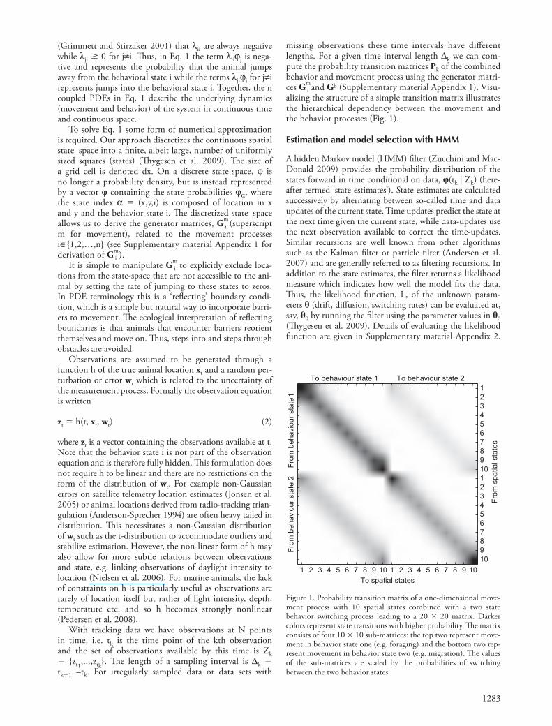
missing observations these time intervals have different lengths. For a given time interval length Dk we can com-pute the probability transition matrices Pk of the combined behavior and movement process using the generator matri-ces Gm

i and Gb (Supplementary material Appendix 1). Visu-alizing the structure of a simple transition matrix illustrates the hierarchical dependency between the movement and the behavior processes (Fig. 1).

Estimation and model selection with HMM

A hidden Markov model (HMM) filter (Zucchini and Mac-Donald 2009) provides the probability distribution of the states forward in time conditional on data, j(tk | Zk) (here-after termed ‘state estimates’). State estimates are calculated successively by alternating between so-called time and data updates of the current state. Time updates predict the state at the next time given the current state, while data-updates use the next observation available to correct the time-updates. Similar recursions are well known from other algorithms such as the Kalman filter or particle filter (Andersen et al. 2007) and are generally referred to as filtering recursions. In addition to the state estimates, the filter returns a likelihood measure which indicates how well the model fits the data. Thus, the likelihood function, L, of the unknown param-eters q (drift, diffusion, switching rates) can be evaluated at, say, q0 by running the filter using the parameter values in q0 (Thygesen et al. 2009). Details of evaluating the likelihood function are given in Supplementary material Appendix 2.

To behaviour state 1 To behaviour state 2

From

spa

tial s

tate

s

To spatial states

From

beh

avio

ur s

tate

2

Fro

m b

ehav

iour

sta

te 1

1 2 3 4 5 6 7 8 9 10 1 2 3 4 5 6 7 8 9 10

1234567891012345678910

Figure 1. Probability transition matrix of a one-dimensional move-ment process with 10 spatial states combined with a two state behavior switching process leading to a 20 20 matrix. Darker colors represent state transitions with higher probability. The matrix consists of four 10 10 sub-matrices: the top two represent move-ment in behavior state one (e.g. foraging) and the bottom two rep-resent movement in behavior state two (e.g. migration). The values of the sub-matrices are scaled by the probabilities of switching between the two behavior states.

1284

V(x, y, t) (t | Z )i 1

n

(x,y,i) N

∑ϕ (4)

which is the probability distribution of the location at time t. Viewing V(x,y,t) in succession for increasing time t (i.e. as an animation) presents an illustrative description of how the location of the animal and its uncertainty changes in time on a day-to-day basis (see Supplementary material Video Appendix for an example). The animation gives particularly important insights when observation errors are non-Gauss-ian or indirect (e.g. of daylight) since in this case the variance of the location is no longer sufficient to describe the spatial correlation patterns.

It is often of interest to examine the amount of time spent by the animal within a spatial region (Walli et al. 2009). As a necessary simplification, previous approaches to calculating the time spent in a region of interest often ignore the fact that the observed location of the animal is uncertain (Aarts et al. 2008). However, Monte Carlo based alternatives incorporating observation uncertainty are available (Sumner et al. 2009). Within the HMM framework the time spent can be expressed as a statistical expectation. At first glance this is not a straightforward calculation because the true locations are always observed with error and, effectively, hidden. Fortunately, the poste-rior distribution can be used to give a reasonable estimate of the time spent at location (x,y) in the time interval t. This time is calculated as the expectation given data and is computed as

R(x, y) (t | Z )l i 1

n

(x,y,i) l N∈τ

ϕ∑∑ (5)

where l indexes time uniformly. This is to avoid that the pos-sibly uneven sample intervals given by the index k lead to a bias in the expectation. Using l means that ϕ(x,y,i)(tl | ZN) must be computed at time points that have no related observa-tion, however at these times the data-update step is simply omitted. So, by summing over the time and behavior indi-ces of the posterior distribution (which incorporate the data induced spatial variability), we get R(x,y) which is a distribu-tional estimate of residence time.

We prefer to normalize R(x,y) and view its cumulative dis-tribution where grid cells are assigned a number between 0% and 100%, so that the 15% contour line, say, contains the smallest region where the animal was expected to spend 15% of its time. This ‘residency distribution’ (RD) is conceptually similar to the utilization distribution (‘UD: The name given to the distribution of an animal’s position in the plane’ cf. Worton 1989). However, as noted by Royle and Dorazio (2008), this and other concepts such as home-ranges (Burt 1943), activ-ity centers etc. (Dixon and Chapman 1980), are often vaguely defined. Despite being notionally similar, the quantity in Eq. 5 should not be directly interpreted as a UD in the usual sense. Nor should it necessarily be related to any sort of home-range, which, in any case, would not make sense for the highly migra-tory animals we consider here (Fig. 3 bottom panel).

In general we may decide to sum over other variables and variable ranges of interest to obtain information about the movement or behavior over a specific time period or for a

Maximum likelihood (ML) estimation of model parameters is then straight forward:

q̂ arg maq

x L(q | ZN) (3)

This optimisation problem can be solved by most stan-dard numerical optimizers which typically also provide an approximation to the Hessian matrix (i.e. curvature) of the likelihood function from which the uncertainty of q̂ can be assessed (Pawitan 2001). For the parameter estimation in this work the optimization toolbox included in Matlab (Mathworks, Natick, USA) was used. In a Bayesian con-text it is common to introduce a priori information about the parameters through the prior density π(q). The maximum a posteriori (MAP) estimate of the parameters is therefore the value of q which maximizes the posterior density L(qZN)π(q). In practice, however, substantial prior information is rarely available (Jonsen et al. 2005) in which case the MAP and the ML estimates are close to identical. Furthermore, for model selection purposes the maximum value of the like-lihood function is required and we therefore use the ML estimate in this study. Selection among alternative models in a Bayesian context would typically employ the Bayesian Information criterion (BIC). Unfortunately, calculating the BIC involves integrals without analytical solutions which therefore must be approximated (Wasserman 2000). The assumptions required by this approximation impose restric-tions on the priors thus reducing the relevance of the BIC in context of the present problem. Instead we calculate Akaike’s information criterion, AIC–2ℓmax2M where ℓmax is the maximum value of the log-likelihood function and M is the number of unknown model parameters. The model having the lower AIC is more likely and therefore ranked higher.

When parameters have been estimated only one step remains which is the so-called HMM smoothing step (Thygesen et al. 2009). The recursions of the smoothing step work backwards in time using the filtered state estimates and all available data to determine the smoothed state estimates, j(tk | ZN). The smoothed state estimates are more accurate and gener-ally appear ‘smoother’ than the filtering estimates because they exploit the full data set (ZN). When fitting an SSM in a Bayesian context the smoothing step provides the posterior distribution of the state. By posterior distribution we mean the probability distribution of all states at all times given all data. Obviously, this distribution has a high dimension and is quite complex. For post-processing purposes it is therefore common to use time marginals of the posterior distribution (i.e. probability distributions of all states at specific times) which, in fact, are the state estimates returned from the HMM smoothing algorithm.

See Supplementary material Appendix 2 for the math-ematical and algorithmic details regarding filtering, smooth-ing, and parameter estimation.

Visualizing results

The posterior distribution obtained from the HMM smooth-ing procedure allows detailed information about behavior and location to be extracted through time. For visualizing details of short-term animal movements we sum the poste-rior distribution over the behavioral state, i.e.

1285

taken from the temperature sensors on the tag. The PSAT was programmed to measure SST and longitude twice per day. However, it was not always the case that the SBT vis-ited the surface in every sample interval. Thus, the returned data were sampled irregularly in time which necessitated a continuous-time analysis.

For the described observation scheme, Eq. 2 becomes

TL

h(t, )t

tt

T

L

æ

èçççç

ö

ø÷÷÷÷÷

æ

èçççç

ö

ø÷÷÷÷÷

xεε

where h is a non-linear function that describes how SST (Tt) and longitude (Lt) inferred from daylight intensity vary as function of location and time. This relation is expressed by hydrographical SST prediction models (six day composite images of remotely sensed SST constructed from advanced very high resolution radiometer (Armstrong and Vazquez-Cuervo 2001), CSIRO Marine and Atmospheric Research) and astronomical models of sunlight exposure (Hill and Braun 2001). Both white noise terms, εT and εL, were assumed to be Gaussian distributed with standard deviations sT 0.71°C and sL 35 km estimated based on inde-pendent data sets (Supplementary material Appendix 5) and were therefore omitted from parameter estimation. For the final results we used a grid size of 111 201 grid cells equat-ing to square cell size of dx 25.52 km. This grid size was limited by computer memory requirements and to keep run times at feasible levels (estimation took 10–40 h depending on the specific model; see below for model configurations).

We considered four movement-behavior models (Table 2) that were different parameter configurations of the SSM and analyzed their relative performance using AIC-based model

specific location. Behavior switching results may be visual-ized by summing over space

B(i, t) (t | Z )x,y

(x,y,i) N∑ϕ (6)

to get the probability of each behavioral state at all time points (Fig. 3 top panel, green line). Viewing B(i,t) with the animation may reveal links between behavior and certain spatial regions (Video appendix VA1, top panel). An alterna-tive approach to relating behavior to space is the expected total time spent in a given region and behavioral state, i.e.

M(x, y, i) (t | Z )l

(x,y,i) l N∈τ

ϕ∑ (7)

These distributions are useful for identifying e.g. migration corridors or residency hot spots while, at the same time, quantifying the spatial uncertainty for these different behav-iors (Fig. 3).

Track estimation is another way to visualize the posterior distribution. A track is an outcome of the posterior distribu-tion and is in the context of this paper defined by a vector a (aT

l,...,aTN). A track in the sense of a not only contains the

estimated geographical coordinates of the animal, but also the most probable switching sequence through the behavior states (Fig. 3 top panel, black line, for an example). Random tracks, conditional on data, can be simulated from the pos-terior distribution as described in Thygesen et al. (2009); this is useful for examining a range of possible tracks and for estimating statistics such as the probability that the indi-vidual enters certain regions. Similarly, the most probable track is the outcome that returns the highest value of the posterior distribution. In technical terms it is a maximum a posteriori estimate, i.e. the state sequence that maximizes the posterior distribution. The probability distribution and the most probable track estimate are different ways of decoding the HMM (cf. Zucchini and MacDonald 2009) and may deviate at times when data are weak (Fig. 3 at the transition from the Tasman Sea to the Southern Ocean).

The algorithm (Viterbi 2006) used to calculate the most probable track is detailed in Supplementary material Appen-dix 3. The performance of the HMM approach with respect to state estimation, parameter estimation and model selec-tion was validated in a simulation study which is in Supple-mentary material Appendix 4.

Data analysis

To demonstrate the described framework, the model was applied to field data from PSATs attached to southern bluefin tuna (SBT) Thunnus maccoyii. Complete details of the data collection procedure are given in (Patterson et al. 2008a). The PSAT (Wildlife Computers PAT-3, Redmond, USA) was deployed on a 168 cm/13 year old SBT captured off the east coast of Australia in the Tasman Sea in July 2003. The known start location was used to initialize the HMM filter. The PSAT detached from the SBT 177 days later, south of Western Australia in the Southern Ocean. Longitude esti-mates (Fig. 2, top) were generated from the PSAT data using the WC-GPE.1.02.0000 software (Wildlife Computers). Mea-surements of sea surface temperature (SST, Fig. 2, bottom) were

Table 2. The four models and their parameter configurations. Model acronyms mean D: diffusion, DA: diffusion–advection, SD: switching diffusion, SDA: switching diffusion–advection.

Model acronym Model parameters No. of parameters

D D1 1DA D1, ux, uy 3SD D1, D2, p11, p22 4SDA D1, D2, ux, uy, p11, p22 6

120

140

160

Long

itude

(°E)

Aug Sep Oct Nov Dec Jan10

15

20

Sea

surfa

cete

mpe

ratu

re (°

C)

Time

Figure 2. The dataset from the southern bluefin tuna as transmitted from the PSAT tag. Top: Longitude as estimated on-board the tag from observed daylight intensity. Bottom: Sea surface temperature measured by the tag when the tuna visited the surface. Notice that data is not sampled uniformly. This is most clear in the final part of the dataset (mid January).

1286

Figure 3 summarizes the movement and behavior estimation for the model with the lowest AIC, i.e. the SDA model. Initially, the SBT resided in the Tasman Sea, east of the Australian continent, for about two months after tag deployment before it moved south to a region northeast of Tasmania. From October and onwards an increased migration probability was apparent (Fig. 3 top panel) as the fish made a westerly migration into the Southern Ocean. The activity level dropped in January as the SBT stayed resident off the Western Australian coast. The RD highlighted four primary areas of residency (Fig. 3 areas A–D). While the RD shown in Fig. 3 is only from a single individual, these areas coincide with apparent residency areas for large SBT from other studies (Patterson et al. 2008a). In the Tasman sea (areas A, B) large SBT have long been targeted by Australian domestic fisheries (Caton 1991). The RD also highlights an appar-ent residency phase in an area off the southern coast of Australia, to the Northwest of Tasmania (area C). This area is known as the ‘Bonnie Upwelling’ (Schahinger 1987) and has been characterized as a local hotspot for a range of predator species, presumably due to the large concentrations of prey species.

Discussion

We presented a hidden Markov model (HMM) as an advanced and versatile approach to state-space modeling. The method provides a unified solution to a number of important complications related to the analysis of move-ment data: the need to explicitly account for movement uncertainty and the entanglement of movement and behav-ior; accounting for barriers to movement; and accommodat-ing multiple sources of non-spatial and possibly irregular data with non-Gaussian error structures. The method can, however, also be useful for mapping behavioral modes present in accurate location data e.g. as recorded by telem-etry devices. Output from the model is calculated using the posterior distribution of the state of the animal. The results therefore have a form that allows detailed biologi-cal insights to be obtained which have not previously been available from tracking data. Additionally, the computa-tion time and accuracy of the solution can be controlled by altering the grid resolution. Thus, coarse results can be obtained rapidly in the implementation phase while final

selection. To maintain focus on the model’s ability to esti-mate behavior we assume that the x and y components of the diffusion terms are uncorrelated. Thus Di diag{[Di,Di]}.

Parameters were estimated for each of the four models listed in Table 2. To ease interpretation we converted the behavior switching rates estimated in continuous-time to transition probabilities for a fixed time step, Dk 0.5 day (12 h). To summarize the movement rate of the SBT we calculated the square root of the expected squared distance moved in a time period of length dt 1 day (24 h):

S E(X ) E(Y )

2D dt (u dt) 2D dt (u dt)i t

2t2

i xi2

i yi2ˆ ˆ ˆ ˆ

which we refer to as the expected movement with unit km day–1. This formula comes from the definition of variance, i.e. that E(A2) V(A) [E(A)]2, where A is a random vari-able. The quantity Si is a useful gauge of the level of activity in behavior state i.

Results

Model selection clearly favored switching models over non-switching models (AIC values in Table 3), a difference which was also highlighted by a 297 km RMS discrepancy between estimated trajectory locations of the diffusion–advection model (DA) and the switching diffusion–advection model (SDA). The estimated values of the advection parameters ux and uy for models DA and SDA were of moderate size and their estimated variance relatively large indicating a reduced influence of these parameters on the tracks and a limited support for these param-eters by the data. Similarly, pairwise comparison of the AIC for the pure diffusion models (D, SD) versus diffusion–advection models (DA, SDA) reported only a slight advantage when the advection parameters were included. However, the SDA model did have the lowest AIC and therefore showed the best fit to data. Estimates of the behavior switching transition rates (pre-sented here as transition probabilities) were almost identical for the two switching models, again supporting the conclusion that the advection contribution to the migratory behavior state for this data was of minor importance. Also the RMS difference in trajectories between the two switching models was small (88 km) and only four locations were classified into different states between the two models. Estimated parameter values and asso-ciated uncertainties are given in Table 3.

Table 3. Results of the data analysis. Maximum likelihood estimates (MLEs) of model parameter values with 95% CI of the four models. Si is the expected movement per day. Unit for Di is km2 day–1, unit for ux and uy is km2 day–1and unit for Si is km.

AICModel D2241.32

Model DA2239.04

Model SD2183.15

Model SDA2180.27

Param. 0.025 MLE 0.975 0.025 MLE 0.975 0.025 MLE 0.975 0.025 MLE 0.975

D1 4923 6644 8365 4873 6739 8605 48 275 502 40 277 514D2 – – – – – – 9519 15439 21360 9391 15577 21763ux – – – –39.6 –22.2 –4.8 – – – –97.4 –53.3 –9.2uy – – – –11.8 5.7 23.1 – – – –33.0 9.3 51.6S1 – 163 – – 166 – – 33 – – 33 –S2 – – – – – – – 248 – – 255 –p11 – – – – – – 0.86 0.95 0.98 0.88 0.95 0.98p22 – – – – – – 0.88 0.95 0.98 0.86 0.95 0.98

1287

the size of a grid cell is smaller than the uncertainty on the estimated position, this limitation is not critical. Also, in many situations discretization of space is actually required and spatially continuous location estimates would need to be discretized post hoc. This applies for example when the objective is to determine residency in a reserve, a habitat patch, or a management unit.

A cogent point for the data considered here is that the precision of an inferred location is much higher than could

results are computed with high accuracy using a fine grid with longer computation times.

Treatments of space and time

A key component of the HMM approach is the need to dis-cretize space. At some level, this requirement may be seen as a limitation since predictions of locations are indeterminate at scales smaller than the model’s spatial units. However, if

Aug Sep Oct Nov Dec Jan0

0.5

1BA C

Mig

ra

tio

n

pro

ba

bility

110°E 120°E 130°E 140°E 150°E 160°E

110°E 120°E 130°E 140°E 150°E 160°E

110°E 120°E 130°E 140°E 150°E 160°E

45°S

42°S

39°S

36°S

33°S

30°S

Ex

pected

p

ro

po

rtio

n o

f tim

e sp

en

t

A

BC

D

Southern Ocean

Tasman Sea

Latitu

de

45°S

42°S

39°S

36°S

33°S

30°S

45°S

42°S

39°S

36°S

33°S

30°S

Latitu

de

Latitu

de

95%

75%

50%

25%

5%

A

BC

D

Southern Ocean

Tasman Sea

Resid

en

t b

eh

avio

rA

BC

D

Southern Ocean

Tasman Sea

Mig

rato

ry b

eh

avio

r

Longitude

D

Figure 3. Top panel: the black line is the most probable behavior switching sequence and the green line is smoothed probability of the migratory behavioral state. Shaded areas relate the behavior switching to the corresponding spatial regions specified in the distribution plots below. Bottom panels: most probable trajectory of the switching diffusion–advection model for the southern bluefin tuna from its release 29 July 2003 to pop-up 22 January 2004. Shaded circles indicate migrating behavior, blue circles indicate resident behavior, green circle is release location and orange square is pop-up location. Underlaid are residency distributions (top: both behaviors, middle: resident, bottom: migratory) showing the expected proportion of time spent by the SBT within the contoured regions. Note that the trajectory deviates from the residency distribution at the migration from the Tasman Sea to the Southern Ocean (details in Methods and Discussion sections). Matlab’s contourf function was used to plot the matrices containing the residency distributions.

1288

Potentially, model structure issues (such as the inclusion of advection terms or not) are important as they may influ-ence inference of biologically relevant quantities, such as estimates of the percentage of time in each behavior mode. For instance, an advection-free model may need to place more locations in the ‘fast’ movement mode to accommo-date directed movement phases. A model with advection may be more flexible and thus able to move the animal faster between locations. However, this did not appear to be a significant factor in the data set we examined. The percent-age of time in the migratory state was only slightly different between the model without advection (9.8% of days) and the model including advection (9.6% of days). Nonetheless, we suspect that further examination of the linkages between model structure, estimation, model selection and subsequent inference of biological quantities is required.

Alternative movement models

As model for individual movement we used variants of Brownian motion, which is the continuous-time equiva-lent to a random walk model. The correlated random walk (CRW) is an alternative model, which is able to capture short-term persistence in the animal’s movement direction (Codling et al. 2008). Thus, the CRW is expected to provide more realistic uncertainty contours for the estimated loca-tions as compared to the Brownian motion. Yet for relatively accurate data an estimated movement path is largely deter-mined by the observations and relies to a smaller extent on the specific model for movement, while for inaccurate data it is not possible to reliably estimate small-scale correlations in movement. Therefore, for the type of data presented here it is unlikely that the estimated overall movement would change significantly if estimated using a CRW instead of the advec-tion-diffusion model. Implementing a CRW in the HMM framework is theoretically possible, but requires gridding of four state dimensions (two-dimensional space and velocity), which entails a substantial total number of states. Even if the velocity can be coarsely discretised, memory requirements and calculation time of a CRW HMM will be immense and possibly impractical.

The Lévy walk (LW, random walk with Lévy distrib-uted steps) is another movement model which has received much attention from ecologists (Sims et al. 2008). It has been argued that LWs in certain scenarios represent the optimal search strategy for animals (Viswanathan et al. 1999). However, theoretical studies have shown (Plank and Codling 2009) that Lévy type movement patterns may arise by sub-sampling of composite random walks (similar to the switching model presented here) and vice versa. Similarly, theoretical results of another study (Thygesen and Nielsen 2009) showed that even if the animal does follow a LW, estimation based on a simple random walk will give only marginally poorer estimation accuracy. Using real data, the state-space and model selection framework we have presented could in a future study be used to compare the estimation performance of switching models versus Lévy models while accounting for observation uncertainty. Such an assessment, while outside the scope of this study, would provide useful insights, for example into the ecological relevance of LWs through statistical tests at the individual animal level.

be inferred from the data alone. Conversely, the scale of the spatial units in the model is much smaller than the scale of migrations made by the animal. Moreover, in this method, barriers to movement are easily included simply by setting the probability of moving to or through impossible locations to zero. Thus any loss of realism stemming from spatial dis-cretization may be offset by ruling out impossible behaviors such as fish crossing land or terrestrial animals crossing large bodies of water. Therefore, the utility of this approach is not significantly diminished by spatial discretization and in fact may offer an integrated approach to aggregating location estimates up to larger spatial scales.

The primary factor influencing the computing time of the method is the grid resolution. Other important fac-tors are the number of behavioral states, the number of parameters to be estimated, and the values of movement parameters. The parameter values are influential because they determine the sparsity of the probability transition matrices (larger values lead to denser matrices and there-fore more computations). With the grid used for our final results the filter requires about one minute to run for the switching model with advection and reasonable parameter values. Total time required for estimation of parameters, tracks, and residency distributions is about a day. If par-allel computing facilities are available more models can be estimated simultaneously thus avoiding extra comput-ing time. The switching HMMs presented here operate in continuous time. Electronic tag data is often subject to regular or irregular gaps in the data stream. As other authors have pointed out (Johnson et al. 2008, Patterson et al. 2010) continuous-time methods handle this seam-lessly. Given that PSAT data is actually a regular time series (twice daily locations) with gaps, a discrete-time approach which handled missing data could equally have been applied. However, the continuous-time approach is more general.

Behavior models and model selection

Model selection for switching Brownian motion models is a challenging process. The simulation study (Supplementary material Appendix 4) confirmed that the correct model was selected if it were present in the candidate set. Predictably, for the analysis of a real data set the situation was not so clear cut. For the SBT track the most complex model (two-state with advection) was ranked highest. From an ecological standpoint, a constant advection term is unlikely to model movement behavior consistently. Future work should, there-fore, consider some of the more advanced models that can be formulated within the state-space framework. While this excludes mechanistic approaches for which a model likeli-hood cannot be computed, a viable future step could be to incorporate time-varying advection in the Brownian motion model. For example, models including constant advection can be rejected when directed movements are present, yet do not exhibit an overall trend through time. In this case a con-stant advection term would most likely be estimated close to zero. Such a result would not however, entail the absence of advective processes in the tuna’s motion but stems from positing sub-optimal models. Then, to incorporate the com-plexity of the observed movement, the diffusivity parameters Di, could end up being spuriously large.

1289

or activity centers, from the model given here, one would use the MPT and treat this as a known set of locations with-out error. Then, kernel smoothing (Breed et al. 2006) or some other approach (Gitzen et al. 2006) could be used for a given sample of MPTs from multiple animals. However, doing this would neglect the uncertainty in the animal’s true locations. Instead, specialized methods for calculating UD (Benhamou and Cornélis 2010) which also incorporate barriers to movement may be considered. In calculating the RD, it may also be useful to marginalize over specific peri-ods of the track. For instance, a researcher may be interested in determining spatial residency of tagged animals over a particular month. Also, the RD may be calculated with respect to specific behavioral states in order to assess which areas are most important as either residency areas or migra-tion corridors (Fig. 3). Finally, by jointly considering the RD from multiple animals it is possible to assess the degree of overlap in their movement paths while simultaneously accounting for uncertainty. These sorts of approaches could be used to large tracking data sets and serve as an advanced alternative to common kernel density estimation methods (Walli et al. 2009).

Conclusion

This paper has demonstrated advances to state-space methods for behavioral estimation. The HMM approach can simultaneously estimate movement parameters, most likely behavioral state, the most-probable track and dem-onstrates how some basic model selection and inference may be carried out. Importantly, the paper provides a method for computing an index of residency which explic-itly accounts for the uncertainty and auto-correlation in both location and behavior. This is an important and often neglected aspect of studies which examine the distribution of animals in space and time using telemetry and elec-tronic tracking data.

Acknowledgements – Karen Evans provided valuable advice and support to this research. Funds were contributed by the Australian Fisheries Management authority.

References

Aarts, G. et al. 2008. Estimating space-use and habitat preference from wildlife telemetry data. – Ecography 31: 140–160.

Andersen, K. H. et al. 2007. Using the particle filter to geolocate Atlantic cod (Gadus morhua) in the Baltic Sea, with special emphasis on determining uncertainty. – Can. J. Fish. Aquat. Sci. 64: 618–627.

Anderson-Sprecher, R. 1994. Robust estimates of wildlife location using telemetry data. – Biometrics 50: 406–416.

Armstrong, E. and Vazquez-Cuervo, J. 2001. A new global satellite-based sea surface temperature climatology. – Geophys. Res. Lett. 28: 4199–4202.

Benhamou, S. and Cornélis, D. 2010. Incorporating movement behavior and barriers to improve kernel home range space use estimates. – J. Wildlife Manage. 74: 1353–1360.

Breed, G. A. et al. 2006. Sexual segregation of seasonal foraging habitats in a non-migratory marine mammal. – Proc. R. Soc. B 273: 2319–2326.

Our primary focus of this study was on behavior and resi-dency estimation, and therefore we employed simple isotro-pic diffusive schemes in the simulation and real data analyses. Naturally, this is a simplification since anisotropic diffu-sion is likely particularly in the presence of advective terms (Codling et al. 2010). Thus, using the HMM approach pre-sented here, or alternative state-space modelling frameworks, to test the statistical significance of anisotropic diffusion with a larger movement dataset would be an interesting topic in future studies.

Spatial patterns

Calculation of most-probable tracksThe most probable track (MPT) is an example of ‘global decoding’ (Zucchini and MacDonald 2009) of the HMM and seeks to find the most likely path given the entire data series taken simultaneously. So-called ‘local decoding’ would involve taking the most likely state from the smoothed time marginal distributions at any particular point in time. Which is used depends on the goal for the inference. For calculating a track the MPT is the most useful, however it can produce some unexpected results. For example, in Fig. 3 the MPT at times deviated from the path that would result from simply choosing the maximum of the time marginal distributions of locations at each time. This can happen when the data for a particular time are uncertain. In this instance the MPT assigns more weight to the distributions from times before and after, and accordingly down-weights the uncertain inter-vening distribution. In such cases, the movement model dominates the MPT and minimizes the rate of movement (depending on the estimated values). The analysis shown here demonstrates that this phenomena may be particularly apparent during migration phases.

One further, useful aspect of the MPT for behavioral switching models is that it avoids the need for ad hoc thresholds for deciding on a most likely behavioral mode. For example, Jonsen et al. (2007) used 0.25 and 0.75 as threshold probabilities for foraging and searching states, respectively.

Mapping spatial uncertaintyOur estimation procedure is Bayesian and therefore gives an estimate of the posterior distribution i.e. the probabil-ity distribution of the animal’s location and behavior. Hav-ing access to the posterior we can calculate the ‘residency distribution’ (RD). As discussed previously, the RD is con-ceptually, and to a degree mathematically, similar to the eco-logical concept of a utilization distribution (UD). However, the RD, as specified here, gives the expected total time the animal visits a location. This is different to other measures such as the UD which assumes that the data provide a rep-resentative (and accurate) snapshot of the distribution of an animal in space. Our RD, on the other hand, accounts for the spatial uncertainty of an animal (Fig. 3) and therefore has certain similarities to the time spent estimation of Sum-ner et al. (2009) although the computational approach is fundamentally different. Whilst the RD and UD are indeed different quantities, the RD has implications for making spatial inferences from uncertain spatial data. To obtain the UD, usage maps (Matthiopoulos 2003, Aarts et al. 2008),

1290

Patterson, T. et al. 2009. Classifying movement behaviour in relation to environmental conditions using hidden Markov models. – J. Anim. Ecol. 78: 1113–1123.

Patterson, T. et al. 2010. Using GPS data to evaluate the accuracy of state–space methods for correction of Argos satellite telem-etry error. – Ecology 91: 273–285.

Pawitan, Y. 2001. In all likelihood: statistical modelling and infer-ence using likelihood. – Oxford Univ. Press.

Pedersen, M. W. et al. 2008. Geolocation of North Sea cod (Gadus morhua) using hidden Markov models and behavioural switching. – Can. J. Fish. Aquat. Sci. 65: 2367–2377.

Pedersen, M. et al. 2011. Nonlinear tracking in a diffusion process with a Bayesian filter and the finite element method. – Comput. Stat. Data An. 55: 280–290.

Plank, M. and Codling, E. 2009. Sampling rate and misidentifica-tion of Lévy and non-Lévy movement paths. – Ecology 90: 3546–3553.

Royle, J. and Dorazio, R. 2008. Hierarchical modeling and infer-ence in ecology: the analysis of data from populations, meta-populations and communities. – Academic Press.

Schahinger, R. B. 1987. Structure of coastal upwelling events observed off the southeast coast of South Australia during February 1983 – April 1984. – Aust. J. Mar. Freshwater Res. 38: 439–459.

Sibert, J. et al. 1999. An advection–diffusion-reaction model for the estimation of fish movement parameters from tagging data, with application to skipjack tuna (Katsuwonus pelamis). – Can. J. Fish. Aquat. Sci. 56: 925–938.

Sims, D. W. et al. 2008. Scaling laws of marine predator search behaviour. – Nature 451: 1098–1102.

Sumner, M. et al. 2009. Bayesian estimation of animal movement from archival and satellite tags. – PloS One 4: e7324.

Thygesen, U. H. and Nielsen, A. 2009. Lessons from a prototype geolocation problem. – In: Nielsen, J. et al. (eds), Tagging and tracking of marine animals with electronic devices. Springer, pp. 257–276.

Thygesen, U. H. et al. 2009. Geolocating fish using hidden Markov models and data storage tags. – In: Nielsen, J. et al. (eds), Tagging and tracking of marine animals with electronic devices. Springer, pp. 277–293.

Vincent, C. et al. 2002. Assessment of Argos location accuracy from satellite tags deployed on captive gray seals. – Mar. Mammal Sci. 18: 156–166.

Viswanathan, G. et al. 1999. Optimizing the success of random searches. – Nature 401: 911–914.

Viterbi, A. J. 2006. A personal history of the Viterbi algorithm. – IEEE Signal Proc. Mag. 23: 120–142.

Walli, A. et al. 2009. Seasonal movements, aggregations and diving behavior of Atlantic bluefin tuna (Thunnus thynnus) revealed with archival tags. – PLoS One 4: e6151.

Wasserman, L. 2000. Bayesian model selection and model averaging. – J. Math. Psychol. 44: 92–107.

Worton, B. 1989. Kernel methods for estimating the utilization distribution in home-range studies. – Ecology 70: 164–168.

Zucchini, W. and MacDonald, I. 2009. Hidden Markov models for time series. – Chapman and Hall/CRC.

Burt, W. 1943. Territoriality and home range concepts as applied to mammals. – J. Mammal. 24: 346–352.

Caton, A. E. 1991. Review of aspects of southern bluefin tuna biology, population and fisheries. – Inter-Am. Trop. Tuna Comm. Spec. Rep 7: 181–350.

Codling, E. et al. 2008. Random walk models in biology. – J. R. Soc. Interface 5: 813–834.

Codling, E. et al. 2010. Diffusion about the mean drift location in a biased random walk. – Ecology 91: 3106–3113.

Cooke, S. J. et al. 2004. Biotelemetry: a mechanistic approach to ecology. – Trends Ecol. Evol. 19: 334–343.

Dixon, K. and Chapman, J. 1980. Harmonic mean measure of animal activity areas. – Ecology 61: 1040–1044.

Gitzen, R. et al. 2006. Bandwidth selection for fixed-kernel analysis of animal utilization distributions. – J. Wildlife Manage. 70: 1334–1344.

Grimmett, G. and Stirzaker, D. 2001. Probability and random processes. – Oxford Univ. Press.

Harvey, A. 1992. Forecasting, structural time series models and the Kalman filter. – Cambridge Univ. Press.

Hill, R. and Braun, M. 2001. Geolocation by light level. – In: Sibert J. R. and Nielsen J. L. (eds), Electronic tagging and tracking in marine fisheries. Kluwer, pp. 315–330.

Ibe, O. 2009. Markov processes for stochastic modeling. – Academic Press.

Johnson, D. S. et al. 2008. Continuous-time correlated random walk model for animal telemetry data. – Ecology 89: 1208–1215.

Jonsen, I. D. et al. 2005. Robust state–space modeling of animal movement data. – Ecology 86: 2874–2880.

Jonsen, I. D. et al. 2006. Robust hierarchical state-space models reveal diel variation in travel rates of migrating leatherback turtles. – J. Anim. Ecol. 75: 1046–1057.

Jonsen, I. D. et al. 2007. Identifying leatherback turtle foraging behaviour from satellite telemetry using a switching state-space model. – Mar. Ecol. Prog. Ser. 337: 255–264.

Matthiopoulos, J. 2003. Model-supervised kernel smoothing for the estimation of spatial usage. – Oikos 102: 367–377.

Morales, J. M. and Ellner, S. P. 2002. Scaling up animal movements in heterogeneous landscapes: the importance of behavior. – Ecology 83: 2240–2247.

Morales, J. et al. 2004. Extracting more out of relocation data: building movement models as mixtures of random walks. – Ecology 85: 2536–2445.

Nielsen, A. et al. 2006. Improving light-based geolocation by includ-ing sea surface temperature. – Fish. Oceanogr. 15: 314–325.

Okubo, A. 1980. Diffusion and ecological problems: mathematical models. – Springer.

Ovaskainen, O. 2004. Habitat-specific movement parameters estimated using mark–recapture data and a diffusion model. – Ecology 85: 242–257.

Patterson, T. et al. 2008a. Movement and behaviour of large southern bluefin tuna (Thunnus maccoyii) in the Australian region determined using pop-up satellite archival tags. – Fish. Oceanogr. 17: 352–367.

Patterson, T. et al. 2008b. State–space models of individual animal movement. – Trends Ecol. Evol. 23: 87–94.

Supplementary material (available online as Appendix O19044 at www.oikosoffice.lu.se/appendix). Appendix 1–5.