Estimating Germany's Potential Output

Working Paper

2/2007

Gustav Horn, Camille Logeay, Silke Tober Macroeconomic Policy Institute (IMK)

in the Hans Boeckler Foundation

ESTIMATING GERMANY’S POTENTIAL OUTPUT

Hans-Böckler-Straße 39 D-40476 Düsseldorf Germany Phone: +49-211-7778-331 [email protected] http://www.imk-boeckler.de

ESTIMATING GERMANY’S POTENTIAL OUTPUT

Gustav Horn, Camille Logeay, Silke Tober1

January 2007

Abstract

Potential output measures a country’s attainable aggregate living standard and is thus one of the most important categories of economics. It is also a key indicator for monetary and fiscal policy. Despite its prominence, how-ever, potential output is a difficult concept to pinpoint both theoretically and even more so empirically. The article discusses the reasons for the marked revisions of potential output estimates by major international or-ganizations. We then present the results of our attempts to quantify Ger-many’s potential output based on a production function approach coupled with the Kalman-filter technique to estimate the NAIRU. We find that po-tential output and potential output growth greatly depend on how the NAIRU and potential total factor productivity are modelled. Given the dif-ficulties involved in robustly estimating potential output, especially in real time, economic policy makers need to learn to pursue their policy objec-tives without reference to this variable.

1. Introduction

Potential output measures a country’s attainable aggregate living standard and is thus one of the most important categories of economics. It is also a key indicator for monetary and fiscal policy. The ECB, for example, uses the output gap – the relative difference between potential output and GDP – as a leading indicator of inflation and requires a precise growth rate of potential output to determine its reference value for M3. Potential output is also relevant for fiscal policy and medium-term fiscal planning, to determine, for example, the structural budget deficit. Despite its prominence, however, potential output is a difficult concept to pinpoint both theoretically and even more so empirically.

In this article we present the results of our attempts to quantify Germany’s potential out-put. Section 2 highlights the theoretical difficulties of unambiguously defining potential out-

1 Paper presented at the workshop “Potential Output and Economic Policy in Europe” organized

by the German Federal Ministry of Economics and Technology in Brussels on 21 September 2006.

1

Horn, Logeay, Tober (2007)

put. Section 3 discusses the reasons for the marked revisions of potential output estimates by major international organizations. Section 4 then presents our own estimates of Germany’s potential output using a production function approach coupled with the Kalman-filter tech-nique to estimate the NAIRU. We find that potential output and potential output growth greatly depends on how the NAIRU and total factor productivity are modelled. In section 5 policy conclusions are drawn from the resulting inexactness and unreliability of potential output estimates.

In the literature the unreliability of real time potential output estimates became a topic of research beginning at the turn of the decade, pioneered by Orphanides (1998) and Smets (1998). Döpke (2004) examines the problem using German data. They attribute the unreli-ability to the endpoint problem, as do we. Our focus is slightly different, however, as we attempted to mitigate the endpoint problem by estimating the crucially important total factor productivity (TFP) using an equation rather than a filtering method or trend estimate. Similar TFP estimates can be found in the literature (for example Denis et al. 2004: 47-48). Unfortu-nately we find that this modification does not reduce the unreliability of potential output estimates by much; nor does the inclusion of exogenous variables when estimating the NAIRU. However, again the focus is different, as we are concerned with the unreliability or arbitrariness of the estimates. The same applies to our NAIRU estimate, which is not a nov-elty, despite the use of exogenous variables. NAIRUs have been estimated by all interna-tional organizations (see, for example Denis et al. 2002, Turner et al. 2001 and International Monetary Fund 2001). Our resulting scepticism concerning potential output estimates does not lead us to advocate the difference rule suggested by Orphanides/Williams (2002) nor to advise that is better “to err on the side of caution” when using output gap estimates (Euro-pean Commission 2002: 9). Rather we support Smets (1998) and others in arguing that un-certain output gap estimates should receive low or rather no weight in economic policy deci-sions. We argue that monetary policy – in order to remain preemtive – should rather focus on the development of wages costs and especially unit labour costs.

2. Potential output in a theoretical perspective

Potential output is the sustainable level of real (inflation-adjusted) GDP. It is constrained due to limited natural resources (population, raw materials), institutional factors (e.g. on labor markets) and the factor endowment (especially the capital stock and human capital). A given level of output is sustainable if it does not generate inflationary or deflationary tendencies. Arthur M. Okun, who coined the term potential output in 1962, defined it as the level pro-duction at full employment, the latter according to Okun referring to the degree of utilisation of the factors of production that does not cause inflationary pressure. In a market economy the concept of potential output necessarily implies an unemployment rate greater than zero. Therefore its analysis also requires analysis of this “equilibrium” unemployment rate, the

2

Estimating Germany’s potential output

non-accelerating inflation rate of unemployment (NAIRU). Okun, for example, calculated potential GDP in an ad hoc manner on the basis of an unemployment rate of 4 % (Okun 1962: 98).

The concept of a sustainable level of output devoid of inflationary and deflationary tenden-cies is much older than the terms „sustainable“, potential output“ and „NAIRU“. More than a century ago Wicksell (1936 [1898]) in his analysis of the “natural” rate of interest asserted that the ratio of output to potential output affects the price level and that inflation theory must analyse the development of aggregate demand and supply. Although Wicksell did not use the term potential output or the term “natural” output level, the concept is obviously implicit in his analysis. And Joan Robinson (1962: 88f.) emphasized that “if we ever reached and maintained a low level of employment, with the same institutions of free wage bargain-ing and the same code of proper behaviour for the trade unions that then obtained, the vi-cious spiral of rising prices, wages, prices would become chronic."

The NAIRU2 may be affected not only by institutional factors, but also by macroeco-nomic policy as indicated by the quote below.

“In some countries, such as the United States, the rise in unemployment was transitory; in others, including many European countries, the NAIRU rose and has remained high ever since. I argue that the reaction of policymakers to the early 1980s recessions largely explain these differences. ... In countries where unemployment rose permanently, it did so because policy remained tight in the face of the 1980s recessions.” (Ball 1999: 190)

The theoretical difficulties of unambiguously defining potential output are due to divergent opinions about the persistency of output gaps and the possible endogeneity of potential out-put, both of which arise from different assumptions about the inherent stability of the econ-omy. From a Keynesian perspective the effectiveness of endogenous mechanisms that return the economy to a given equilibrium is uncertain at best.3 Longer-lasting negative output gaps are thus a likely occurrence and entail the danger of hysteretic effects causing potential out-put to adjust to the GDP rather than vice versa. In contrast, monetarists and proponents of new classical theory hold the view that the rational behaviour of economic agents rapidly corrects disequilibria and that potential output is unaffected by economic downswings and upswings. New Keynesians occupy a position somewhere in between. Economic policy ad-vice differs in accordance with these divergent views. Whereas Keynesians tend to favour active macroeconomic stabilisation policies and regard macroeconomic policy as a necessary adjunct to structural reform, monetarists and new classical theorists view macro policy as

2 The NAIRU concept was developed by Modigliani and Papademos (1975), who, however,

called it NIRU (noninflationary rate of unemployment). The term NAIRU was first used by Tobin (1980). Unlike the term “natural rate of unemployment” introduced by Friedman in his Presidential Address to the American Economic Association in 1968, the NAIRU is not a purely neoclassical con-cept; see Carlin / Soskice (1990: 166).

3 See, for example, Bean (1997), Spahn (1997), Tobin (1993), Greenwald/Stiglitz (1993), Pat-inkin (1992, Leijonhufvud (1990), Riese (1986), Blanchard/Summers (1986), Keynes (1936/1964).

3


more or less superfluous, argue strongly for rule-based policies, and consider structural re-forms to be the key to higher economic growth.

An output gap that persists over a long period is unlikely from a theoretical perspective. Eventually capital stock adjustments (Bean 1997: 93; Gordon 1997: 439) and hysteresis on the labor markets4 will lower potential output until the gap disappears. Underutilization of capital is small if it exists at all and the long-term unemployed may not be hired at the going wage even if aggregate demand picks up. Since monetary policy is generally believed to be powerful enough to cause output gaps in the short and medium run, the implication for monetary policy is apparent: if output gaps close as a result of labour market hysteresis and capital stock adjustments, then macro policy is not neutral in the long run but rather affects the real economy.

“…If monetary policy can affect real economic activity by means other than money illu-sion then it may be possible for money to be nonsuperneutral in the long run.”

Espinosa-Vega (1998: 13)

In addition to the NAIRU, endogenous technological progress is a second channel through which macro policy may affect the level of potential output.

3. Revisions of Germany’s potential output

From an empirical perspective it is also the NAIRU and endogenous technological progress that make it difficult to estimate and forecast potential output with certainty. Volatile out-comes resulting from small changes in the specification or the estimation period pose a prob-lem for policy makers because estimation errors can have dire consequences for unem-ployment and inflation.

Methods to estimate potential output can be categorised into three groups: first, purely statistical methods (eg. Hodrik-Prescott filter and Rotemberg filter); second, methods that determine potential output primarily on statistical grounds but make use of the interaction between certain economic variables (semi-structural methods, eg. multivariate Hodrick-Prescott filter and multivariate Kalman filter); and third, methods that determine potential output on the basis of economic factors (structural methods, eg. production function ap-proach). Only structural methods make possible a distinction between different theoretical approaches. They are also better suited for projections and simulations exercises, especially in the case of changes in the structural or macroeconomic environment at the end of the ob-servation period. They are superior to univariate methods because they provide an economic explanation of movements in potential output.

4 See Logeay/Tober (2006) for an overview of causes of labor market hysteresis.

4


Output gap in % of potential output

IMF estimates at different points in time1

1 Real time is the output gap estimate for the year preceding the publication year

Sources: International Monetary Fund, World Economic Outlook, spring issues 1994 to 2006.

-4

-3

-2

-1

0

1

2

1993 1997 2001 2005WEO April 2000 Real time WEO April 2006

In practice, however, estimates based on production functions are to a large ex-tent based on univariate methods, especially the Hodrick-Prescott filter, to estimate the potential values of the individual components of the production function. It is therefore not surprising that the estimates of potential output of different institutions are quite similar and actually more similar than are the estimates of each institution for a specific year at different points in time. In the case of the International Monetary Fund (IMF) this difference can be exemplified best using the years 1999 and 2001. In the spring 2000 the IMF estimated Germany’s output gap in 1999 to be -2.8 %; in the spring of 2006 the

IMF puts the output gap in 1999 at +0.1 %: this is not only a difference of almost 3 percentage points but also a change from negative to positive. The real-time estimate of Germany’s output gap in 2001, i.e. the estimate in the spring of 2002, was -1.2 %; from to-day’s perspective (spring 2006) the IMF estimates the output gap in 2001 to have been 1.5 % and thus markedly positive. An equally stark picture emerges when looking at the figures provided by the EU Commission and the OECD.5 Revisions of this magnitude invalidate the use of measures of output gaps and potential output growth as indicators for economic pol-icy. To illustrate the problem we calculated Germany’s output gap for 2005 on the basis of the rate of potential growth that the IMF estimated in spring 2000 for period from 1992 to 2001, that is 2.1 %.6 According to this calculation the output gap in 2005 would have ex-ceeded 8 %.7

The frequent and large potential output revisions are largely due to the econometric methods used for estimating potential output, in particular the endpoint problem and forecast mistakes, rather than to data revisions or a changing view of underlying structural factors. Below we show how revisions come about by estimating the potential labor force, potential

5 See also Orphanides and Williams (2002) as well as Döpke (2004), who analyse this discrep-

ancy between potential output estimates in real time and in retrospect for the United States and for Germany, respectively.

6 The potential growth rate deviates from 2.1 % in only two years, namely in 1995 (2.0 %) and in 1998 (2.2 %). This is probably due to rounding errors.

7 This calculation is meant to be illustrative only, since the repercussions of the prolonged eco-nomic weakness on potential output are not considered. The output gap thus calculated cannot be closed immediately but rather only over a period of several years.

5


TFP and the NAIRU based on the following time series of the current AMECO database for the period 1970-2007 and 1970-2000, respectively: real GDP, net capital stock, labor force, standardized unemployment rate, wage share and NAIRU. The time series for West Ger-many and unified Germany are linked using growth rates. We then calculate the average wage share (62 %) and – by rearranging the production function equation – a time series for total factor productivity (TFP). First, we apply an HP filter on the labor force and on TFP to produce their respective potential values and, subsequently, a series for potential output. Focusing again on the year 2000 we calculate an output gap of +1 %. Second, we go back in time to 2001, a time when the time series above included data up to only 2000. To extend the series until 2007 we apply the two methods most commonly used by international organiza-tions: simple ARIMA models and ad-hoc extensions. In the ARIMA version TFP and labor force are estimated in log levels, more specifically with an AR(2) model with trend and a simple AR(2) model, respectively. The new data points thus generated exceed the trend ob-served in 1995-2000. In contrast, the ad-hoc method extrapolates this trend. The NAIRU is in both cases generated according to the method used by the EU Commission, i.e. we in-crease (decrease) the NAIRU by half of the change in the preceding year. We now recalcu-late potential output based on these data. The time series generated by the AR model yields an output gap of 0.4 % in 2000, the trend-based approach one of -0.3 %.

Our example shows that potential output estimates greatly depend on the expected val-ues of its components which, in turn, largely depend on the respective previous development in the estimation models used.8 It follows that current estimates of Germany’s potential out-put may prove to be far too pessimistic if the economic weakness of the past years proves to be a temporary phenomenon.

8 The revisions are not the result of changes in the data provided by the Federal Statistical Office

or a different interpretation of the existing wage pressure. The revisions of Germany’s growth rates for 1999, 2000 and 2001 amount to 0.5 percentage points, 0.1 percentage points and 0.7 percentage points, respectively. Although these revisions can partly explain the revisions of the output gap, they offer no grounds for downward revisions of potential output (Calculations of the authors based on data provided by the Federal Statistical Office.)

6


Potential growth rates in artificial real time

0.5

1.0

1.5

2.0

2.5

3.0

3.5

0.5

1.0

1.5

2.0

2.5

3.0

3.5

1970 1975 1980 1985 1990 1995 2000 2005

Potential output growth in % (AR model from 2001 on)Potential output growth in % (constant growth rates from 2001 on)Potential output growth in % (data available in 2005 from 2001 on)

4. IMK estimates of Germany’s potential output

Like most international organisations we use a production function approach to estimate potential output in Germany. The NAIRU is estimated using a Kalman filter. For various reasons we stick relatively close to the modelling strategy of the EU Commission (Denis et al. 2002), one being its relevance for the national governments in the Euro Area when, for instance, formulating their stabilisation programmes. One important difference is the way in which we calculate the potential level of the components of the production function, namely the NAIRU and total factor productivity.

We estimated the following Cobb-Douglas production function:

Y*t= A*

tL*tα

' K*t1-α ,

where Y* is potential output, A*t potential total factor productivity, L*

t potential hours worked, α the partial elasticity of production with respect to labor and Kt

* the capital stock.

The NAIRU is needed to calculate the potential hours worked. More specifically (1-NAIRU) is multiplied with the potential labor force (HP-filtered actual labor force) to deter-mine the non-inflation-accelerating level of employees. The latter is then multiplied with average potential working time (HP-filtered actual average working time) to calculate poten-tial hours worked. The coefficient α is equated with the average wage share in the given period (0.65). The potential capital stock is taken to be identical with the actual capital stock. Potential total factor productivity (A*

t) is then determined by first solving the production

7


function for At using actual employees and actual GDP rather than their potential levels. This TFP is then estimated as dependent on several determining factors. Potential total factor productivity is calculated by plugging the potential levels of these factors into the equation. In the following we first describe the data used and then present our estimates of the NAIRU, total factor productivity, and potential output.

4.1 Data sources

We mainly use annual data provided by the German Federal Statistical Office (Destatis). These are by and large identical to the data used by the EU Commission. When this paper was written, no official time series for the German capital stock existed, so we used the EU Commission’s time series, adjusted using time series for depreciation and gross fixed in-vestment to make it compatible with the German system of national accounts. Furthermore we use the standardized unemployment rate provided by Destatis on an annual basis, by the OECD on a quarterly basis. We deal with German unification, as does the EU Commission, by linking the time series in growth rates thus calculating (artificial) levels prior to 1992. Institutional variables used in estimating the NAIRU are taken primarily from the dataset of Nickell et al. (2001),9 Bassanini/Duval (2006), the OECD’s databank, Martinez-Mongay (2000, 2003), Destatis, AMECO and Visser (2006). Nickell et al. (2001) provide a time series on employment protection which we extended beyond 1995 using data from Bassan-ini/Duval (2006), the last two data point were estimated making adjustments for various reforms.10 The Nickell et al. (2001) time series on union density was extended using data from Visser (2006), the last year is our estimate based on the assumption that the decreasing trend continued. We continued the series on replacement rates provided by Bassanini/Duval (2006) with two estimated data points, taking into account that replacement rates are lower in 2005 due to the partial merging of welfare benefits and unemployment benefits (Hartz-IV reform) and that the OECD’s net replacement ratio registered a decrease for all household groups in 2004. For the wage wedge we used two different time series: the first is the abso-lute difference between compensation of employees and net wage sum in percent of compen-sation of employees (national accounts data). The second series is an updated version of the effective tax burden (taxes, duties, social security contributions) on labor as calculated by the EU Commission (Martinez-Mongay 2000 and 2003). It is the ratio of the sum of non-wage labor costs and wage tax to gross wages and salaries. The monetary indicators used to esti-mate the NAIRU are based on data from the German Bundesbank. The overnight rate and “indicator of the German economy’s price competitiveness against 19 countries based on the deflators of total sales” were used as provided by the Bundesbank. The real short-term inter-est rate is the overnight rate minus the change in the GDP deflator, the latter calculated on the basis of the Destatis time series on real and nominal GDP (before 1992: West Germany).

9 Labor Market Institutions Database (LMID), Online access: http://cep.lse.ac.uk/pubs/author.

asp? author=nickell. 10 Cf. Deutsche Bundesbank (2005: 25) for an overview of these reforms.

8


To estimate total factor productivity we used as additional data sources the Congressional Budget Office (U.S. potential total factor productivity), AMECO database, OECD Main Science and Technology Indictors (per capita expenditure on research and development) as well as Ifo and OECD (capacity utilization in manufacturing).11

4.2 The NAIRU

4.2.1 Kalman-filter estimate of the NAIRU

The problem with estimating the NAIRU is that it an unobservable variable. The Kalman-filter approach was developed specifically to estimate such variables and it has the advantage over univariate filter methods that it links the unemployment gap to some measure of infla-tion. In that sense it satisfyies the definition of the NAIRU and gives the estimate economic content. In addition, it is possible to estimate the influence of exogenous factors, such as monetary policy. It should be noted, however, that the results of the Kalman-filter estimate strongly depend on the specification of the estimated equations. For example, the fact that the NAIRU is specified as an AR(2)-process implies that it is necessarily a stationary vari-able. Although this is a sensible assumption, it would have been preferable to find this char-acteristic as a result rather than plugging it in as an assumption. An alternative method based on fewer assumptions is the Elemeskov method that the OECD used until a few years ago. Unfortunately the estimated NAIRU is so volatile, that one is forced to use a HP-filter or the like to obtain a sensible time series. The HP-filtered Elemeskov NAIRU, however, is hardly distinguishable from a plain HP-filtered NAIRU, leading us to reject this approach.

To estimate the unobservable NAIRU with the Kalman filter it is necessary to make an assumption about how the NAIRU interacts with other economic variables that are observ-able as well as the time series properties of the NAIRU and, in this case, the output gap. We estimate the NAIRU as a nonstationary trend (time series property), more precisely as a local linear model,12 and assume that the unemployment gap (u-u*) significantly affects inflation. To use the information contained in this economic relation – the Phillips curve – the NAIRU is estimated simultaneously with the Phillips curve. The unemployment gap is modeled as an AR(2) process.13

State equations:

(u-u*)t = ar1 (u-u*)t-1 + ar2 (u-u*)t-2 + εugapt

11 Neither the Federal Statistical Office nor the OECD provides a long time series about the edu-

cational attainment of the population. 12 A local linear model is de facto equivalent to a ARIMA(0,2,1). Depending on the variances of

the two error terms it can be either a simple random walk or an I(2) process. Many authors use this approach because it allows for a smooth trend; cf. Harvey und Jaeger (1993).

13 This is a typical way of modeling the unemployment gap; cf. Fabiani/Mestre (2001) and A-pel/Jansson (1999).

9


Nairuimplizitt = Nairuimplizit

t-1 + trendt + εnairut

trendt = trendt-1 + εtrendt

Nairut = Nairuimplizitt + δZnairu

t

Definition equation:

ut = (u-u*)t + Nairut

Phillips curve equation:

∆²wht = β(u-u*)t + γXPhillips

t + εphillipst

Xphillipst denotes exogenous variables that affect hourly wages (wh).

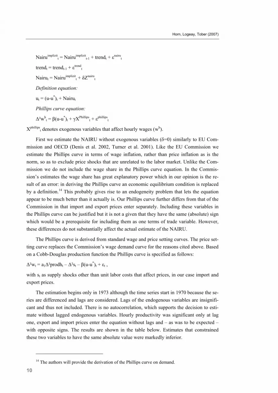
First we estimate the NAIRU without exogenous variables (δ=0) similarly to EU Com-mission and OECD (Denis et al. 2002, Turner et al. 2001). Like the EU Commission we estimate the Phillips curve in terms of wage inflation, rather than price inflation as is the norm, so as to exclude price shocks that are unrelated to the labor market. Unlike the Com-mission we do not include the wage share in the Phillips curve equation. In the Commis-sion’s estimates the wage share has great explanatory power which in our opinion is the re-sult of an error: in deriving the Phillips curve an economic equilibrium condition is replaced by a definition.14 This probably gives rise to an endogeneity problem that lets the equation appear to be much better than it actually is. Our Phillips curve further differs from that of the Commission in that import and export prices enter separately. Including these variables in the Phillips curve can be justified but it is not a given that they have the same (absolute) sign which would be a prerequisite for including them as one terms of trade variable. However, these differences do not substantially affect the actual estimate of the NAIRU.

The Phillips curve is derived from standard wage and price setting curves. The price set-ting curve replaces the Commission’s wage demand curve for the reasons cited above. Based on a Cobb-Douglas production function the Phillips curve is specified as follows:

∆²wt = a1∆²prodht – ∆²st – β(u-u*)t + εt ,

with st as supply shocks other than unit labor costs that affect prices, in our case import and export prices.

The estimation begins only in 1973 although the time series start in 1970 because the se-ries are differenced and lags are considered. Lags of the endogenous variables are insignifi-cant and thus not included. There is no autocorrelation, which supports the decision to esti-mate without lagged endogenous variables. Hourly productivity was significant only at lag one, export and import prices enter the equation without lags and – as was to be expected – with opposite signs. The results are shown in the table below. Estimates that constrained these two variables to have the same absolute value were markedly inferior.

14 The authors will provide the derivation of the Phillips curve on demand.

10


The coefficients can simply be read of the table because there are no lagged endogenous variables: a decline in the output gap by 1 percentage point for one year (three years) perma-nently lowers wage inflation by about 0.5 percentage points (about 1.4 percentage points). A permanent increase in productivity growth by one percentage point permanently raises wage inflation by 0.7 percentage points; at the same time the increase in unit labor costs is perma-nently lowered by 0.3 percentage points. An increase in export price inflation by 1 percent-age point increases wage inflation by 0.4 percentage points, a corresponding increase in im-port prices lowers it by 0.1 percentage points.

The AR-coefficients of the unemployment gap imply an average cycle length of nine years. The unemployment gap is estimated with a small positive constant implying deflation-ary pressure. This is compatible with the three disinflationary periods during the estimation period: The increase in hourly wages diminished from 12 % in the early seventies to 5 % in the late eighties and again since the mid-nineties to nearly 0 % in 2005. The variances of the error terms are not constrained, the local linear model is therefore not a simple random walk (Fabiani/Mestre 2000 and 2001, European Commission 2002 and 2006). The residuals of the NAIRU equation exhibit no autocorrelation. The distribution of the residuals of the Phillips curve is normal, that of the state equations, however, probably not. According to our esti-mate the NAIRU stood at 8.1 % in 2005.

11


Results of the Kalman-filter estimate of the German NAIRU

Variables

State equationsar1 1.264 0.128 9.860ar2 -0.655 0.124 -5.289constant 0.003 0.002 1.145Var(εnairu) 1.88E-04Var(εtrend) 1.95E-04Var(εgap) 2.51-02

Phillips curve(u-u*) -0.462 0.198 -2.327d²prodh(-1) 0.658 0.225 2.927d²pex 0.403 0.192 2.098d²pim -0.127 0.074 -1.713

R² 0.464-2*log-likelihood -418.368Var(εphillips) 1.266E-04

residual tests

State equationsLjung-Box Q(4) statistic 1.463 prob: 83.3%Jarque-Bera statistic 9.599 prob: 0.8%

Phillips curveLjung-Box Q(4) statistic 4.237 prob: 37.5%Jarque-Bera statistic 1.285 prob: 52.6%

Maximum likelihood equation and statisticsestimation periods: 1973-2005 (33 observations)

coefficients s.e. t-stat

12


Kalman-filter estimate of the NAIRU

0

2

4

6

8

10

1970 1975 1980 1985 1990 1995 2000 2005

standardized unemployment rate in %NAIRU in % (Kalman filter without exogenous variables)

The Commission’s GAP program allows us to include exogenous variables in estimating the NAIRU. This approach is somewhat problematic because the state equations are split into three different groups: the unemployment gap, a statistical process (here: local linear model) and the exogenous variables.15 It follows that the exogenous variables can only affect the NAIRU temporarily unless they represent structural breaks. Including lagged unemployment only partly solves the problem since the GAP program then regresses the unemployment rate rather than the NAIRU on the exogenous variables. We therefore applied this one-step Kal-man-filter approach primarily when testing for hysteresis. Institutional and monetary policy variables were, in addition, tested for in a two-step approach: We first estimated the NAIRU with the Kalman filter and then used OLS to regress this NAIRU on the exogenous variables. Compared to other studies using OLS ours has the advantage of using an estimated NAIRU rather than resorting to longer term averages of the unemployment rate like, for example, Blanchard/Wolfers (2000) or forgoing degrees of freedom like Nickell et al. (2002) who include an inflation variable in the regression to exclude cyclical movement.

4.2.1 Exogenous variables

The effects of institutional variables on the NAIRU were tested for using four variables, namely employment protection, union density, replacement rate and wage wedge. These

15 An alternative approach would be to split unemployment into unemployment gap and NAIRU,

the latter in turn being modeled as a function of itself (random walk approach) and the exogenous variables.

13


variables feature greatly in the literature, are available as long time series and largely reflect Germany’s recent labor market reforms. We included the variables in the NAIRU estimation individually and together using both the Kalman filter and OLS. With the exception of the wage wedge,16 the outcomes of the estimations with institutional variables were not robust, being either highly dependent on the specification of the estimated equation or insignificant or bearing the wrong (theoretically implausible) sign. In part this may be due to statistical problems arising from German unification. Furthermore, it should be noted that since the late seventies the examined variables – again with the exception of the wage wedge – should have lowered the German NAIRU if they affected it at all. The limited explanatory power of institutional variables for unemployment is also pointed out in the literature (Blanchard/Katz 1997: 68, Machin/ Manning 1999: 3107, OECD 2006: 214 and Bassanini/Duval 2006: 63). Blanchard/Wolfers (2000:2), for example, argue that

“...many of these institutions were already present when unemployment was low (and similar across countries), and, while many became less employment-friendly in the 1970s, the movement since then has been mostly in the opposite direction. Thus, while labour market institutions can potentially explain cross country differences today, they do not appear able to explain the general evolution of unemployment over time.”

In line with part of the literature monetary policy was also tested for as a factor that af-fects long-term unemployment.17 There is no doubt that the restrictive monetary policy in the late seventies as well as the early eighties and nineties played a big role in the increase of the unemployment rate.18 Whether this effect was only of a short-term nature – thus not affecting the NAIRU – is however quite controversial.19 If monetary policy gives rise to hysteresis in labor markets, for example, and thereby changes the effective labor supply, its short-run effects may extend to the long run. Based on Granger causality tests (Blinder/Bernanke 1992) of various monetary policy indicators and the standardized unemployment rate, we

16 The wage wedge (based on national accounts data) was found to be significant in both the

Kalman-filter estimate and the OLS-estimate. Due to possible endogeneity it was introduced with a lag. The Kalman filter finds a coefficient of 0.18 for the first lag, OLS a comparable one of 0.15. The latter changes only minimally when a different deterministic structure is used. Our results are at the lower end of the range of 0 to 0.6 found in the literature (Planas/Röger/Rossi 2006). The coefficient of 0.18 implies that 2.5 percentage points of the increase in the NAIRU between 1973 and 1998 were the result of a widening wage wedge; since 1998 the wage wedge led to a small reduction in the NAIRU of 0.3 percentage points. In contrast, the wage wedge as calculated in line with the EU Commission was insignificant.

17 Cf. Ball and Mankiw (2002), Ball (1999), Blanchard and Katz (1997) as well as Fitoussi, Jestaz, Phelps, and Zoega (2000), who relate the marked increase in unemployment and the fact that it remained high to the restrictive stance of monetary policy in Europe.

18 Modern monetary policy is based on the notion that money is not neutral in the short term. Nominal rigidities give rise to short-term non-neutrality; cf. Clarida, Galí, and Gertler (1999), McCallum (2001), Mankiw (1985), Akerlof, Dickens, and Perry (2000). In the short term monetary policy is thought to have an effect on real interest rates, aggregate demand and inflation. Unemploy-ment is the key variable through which monetary policy affects inflation (Layard, Nickell, and Jack-man 1991: 13).

19 Contrary to the mainstream view, the view that monetary policy has long-term real effects is put, for example, by Cross (1995) and Ball (1999).

14


used the deviation between the real short-term interest rate and the rate of economic growth. This monetary policy indicator has the advantage of being unaffected by fundamental chan-ges in the real interest rate due, for example, to a change in the potential growth rate. It is superior to the nominal overnight rate because the effects of monetary policy are not inde-pendent of inflation: an increase in interest rates that lags behind the increase in inflation is likely to have an expansionary effect, for example. We analysed the effect of this variable in two different Kalman-filter models and one OLS regression using our Kalman-filter NAIRU. In each case the variable was significant and robust, albeit with a relatively low coefficient of 0.1. As a check we estimated an additional OLS regression in which we determined the long-term monetary policy effect on the unemployment rate directly, rather than its effect on the NAIRU. Conceptually the two are obviously identical. The stationary monetary policy indicator enters the equation in levels, the nonstationary unemployment rate in first differ-ences. The long-term coefficient is here estimated as 0.22 and the results are robust to differ-ent specifications. Our preferred specification was derived using the general-to-specific ap-proach and includes a trend that can be interpreted to proxy omitted variable. It exhibits no econometric problems.

The results of our hysteresis estimates are also robust. Hysteresis can have different causes but the key factor seems to be that the number of long-term unemployed increases and that these influence labour market developments and wages, in particular, less than do the temporarily unemployed. Numerous studies have found empirical evidence for hysteresis (Logeay/Tober 2006; Røed 1997). Our approach is similar to that used by Salemi (1999) and Jaeger/Parkinson (1994) and superior to unit root test (Léon-Ledesma 2002; Léon-Ledesma/McAdam 2004) cointegration (Johansen 1995), lagged unemployment in wage-price systems (Layard, Nickell, and Jackman 1991) and Markov-switching (Léon-Ledesma/McAdam 2004) because it does not require the assumption of a certain invariance of the institutional structure like unit root tests and Markov-switching nor a full specification of the determinants of the NAIRU as do cointegration and panel estimations of wage-price systems.

The time series for long-term unemployment was constructed from two sources. For the period 1983 until 2004 we used OECD data which corresponds more closely to the standard-ized unemployment rate than does the long-term unemployment rate provided by the Federal Employment Agency. The missing years were estimated using data from the Federal Em-ployment Agency and IAB. Several different specifications were used to account for German unification. The best ones included a step or impulse dummy variable for 1991. In both esti-mations the coefficient of the rate of long-term unemployment is 1. Translated into the effect of lagged unemployment, which is often used to measure hysteresis effects, the coefficient is 0.4. Our coefficient is approximately twice as large as that in Jaeger/Parkinson (1994), who apply a similar method but use lagged unemployment and find a coefficient of 0.18 for Ger-many. It does, however, correspond to the coefficient in Jaeger/Parkinson (1990).

15


The fact that the rate of long-term unemployment proved to be significant in the estima-tion of the NAIRU indicates the presence of hysteresis. Hysteresis, in turn, implies that vari-ables will affect the NAIRU if they cause unemployment to stay high or low for a prolonged period. Our analysis thus shows that the unemployment gap and the NAIRU are not inde-pendent of each other: to a certain degree the structure of unemployment hardens or loosens, thus causing the unemployment gap to close partly through an increase or decrease in the NAIRU.

4.2.1 Projecting the NAIRU

Projecting potential output requires that the NAIRU is projected as well. We used three dif-ferent methods to forecast the NAIRU, namely the method employed by the EU Commis-sion, the Kalman filter and an OLS equation with projected values for the exogenous vari-ables wage wedge and monetary policy indicator. Despite the methodological differences the NAIRU projections range only from 8 % to 8.2 %. It follows that the different methods of estimating the NAIRU do not greatly affect the projection of potential output. As indicated above, this does not imply that the projection of the NAIRU is particularly accurate but rather that the statistical characteristics of the NAIRU (and the unemployment gap) – which are identical in all the cases presented here – dominate the results.

It should be noted that the statistical characteristics dominate not only the projection of the NAIRU but also its estimation: The Kalman-filter estimate of the NAIRU using a ficti-tious constant inflation rate for the estimation period yields a time series for the NAIRU that hardly differs from the estimate above. Similarly, the use of a univariate Kalman filter only changes the results by 0.5 % or 0.7 %, depending on the specification used. The chart below shows that the NAIRU estimate is affected more by whether it is modeled as a random walk or as a local linear model than by whether a univariate or a multivariate model is used. There is a difference in the level of the NAIRU, the movement in NAIRU is almost identical, so that although the output gap is affected the effect on potential growth is non-existent.

16


Univariate and multivariate Kalman-filter estimates of the NAIRU

0%

1%

2%

3%

4%

5%

6%

7%

8%

9%

10%

1974 1979 1984 1989 1994 1999 2004

Nairu, multivariat (lokaler linearer Trend) Nairu, univariat (lokaler linearer Trend) Erwerbslosenquote

0%

1%

2%

3%

4%

5%

6%

7%

8%

9%

10%

1973 1978 1983 1988 1993 1998 2003

Nairu, multivariat (Random Walk) Nairu, univariat (Random Walk) Erwerbslosenquote

4.4 Estimate and projection of potential total factor productivity

Potential total factor productivity (TFP*) is the second key variable to be estimated to deter-mine potential output in the production function approach. Unlike the EU Commission (Denis et al. 2005, Carone et al. 2006) we estimated an equation that allows for the total factor productivity to be partly determined by other economic variables, namely the invest-ment ratio, per-capita expenditure on research and development and U.S. total factor produc-tivity.

Because there are only 30 data points we estimated specific to general rather than vice versa. The estimate is in levels although the variables are nonstationary. This is permissible because sufficient lags of each variable are included. An increase in the investment ratio by

17


1 percentage point is estimated to increase total factor productivity by 1.2 %. An increase in expenditure on research and development (per capita) by 1 % raises the TFP by barely 0.1 %. An increase in U.S. TFP by 1 % increases German TFP by 0.9 %. We also find mone-tary policy to have an effect, albeit an indirect one via the investment ratio. An OLS regres-sion with the investment ratio in first differences as dependent variable and the monetary policy indicator as independent variable yields an elasticity of -0.1. According to this esti-mate a three-year monetary restriction keeping the real overnight rate 1 percentage point above the growth rate of GDP, would permanently lower the investment ratio by 0.3 percentage points.

Potential TFP was determined by plugging equilibrium values for the investment ratio and research and development expenditure into the TFP equation. We defined the equilib-rium investment ratio as the average investment ratio during the observation period (21.7 %) which roughly corresponds to the recent investment ratios in the other countries of the Euro Area. The equilibrium path for research and development expenditure was generated with a broken deterministic trend. We distinguished between 4 phases: the seventies with annual per-capita R&D expenditure exceeding 10 %, the eighties when the growth rate was almost half as high; the unification years which saw a decline in the absolute level, and the period since 1995 with relatively low growth rates of 4 to 5 %. For US TFP we took the actual lev-els, because these are assumed to be unaffected by developments in Germany.

Actual, explained and potential TFP1

.04

.05

.06

.07

.08

.09

.04

.05

.06

.07

.08

.09

1970 1975 1980 1985 1990 1995 2000 2005

TFP (alpha = 0.649)Explained TFPPotential TFP

1 Actual TFP is calculated by rearranging the production func-tion, explained TFP is estimated using three exogenous vari-ables and potential TFP is the estimate of TFP with the invest-ment ratio and R&D expenditure in equilibrium.

18


There are different methods for forecasting potential TFP. The EU Commission uses a univariate model to estimate and forecast actual TFP and then an HP-filter to generate an estimate and forecast of potential TFP. Our approach differs in that we use the OLS regres-sion to project potential TFP. The potential investment ratio is again assumed to be 21.7 %, the potential increase of per-capita R&D expenditure 4.6 % which corresponds to the aver-age of the period 1995 to 2004. For the US TFP we use the CBO’s forecast of 1.4 % (CBO 2006). According to the forecast of the EU Commission potential TFP will increase at an annual rate of 0.8 %, the AR model yields 1.5 % and our OLS regression forecasts an annual increase in potential TFP of 1.7 %. It is important to note that in the production function TFP translates one to one into potential output.

4.6 Estimating and projecting potential output

Given the estimates and projections of the NAIRU and TFP we estimated potential output using the following equation:

Yt* = TFPt

* (laborforcet* working timet

* [1-Nairu])0,65 (Kt)1-0,65

Estimates of the German output gap using several NAIRUs and several potential TFPs

-5

-4

-3

-2

-1

0

1

2

3

4

1970 1975 1980 1985 1990 1995 2000 2005

Output gap (HP 100)Output gap (AMECO EU Commission 2006)Output gap (HP for pot. TFP, pot. working time and pot. labor force, K-f Nairu – random walk without driftOutput gap (HP for pot. working time and pot. labor force; K-f Nairu – random walk without drift; pot. TFP - OLS)Output gap (HP for pot. working time and pot. labor force; K-f Nairu – random walk with drift; pot. TFP - OLS)

in %

of p

oten

tial o

utpu

t

The substantial differences between the estimates arise primarily from the different series for potential TFP. At the end of the estimation period our estimates show large negative output gaps resulting from the fact that the recent slowdown in economic activity is not attributed to a change in potential output growth.

Potential output was then projected using the following equation: Yt* = TFPt

* (labor for-cet

* working timet* [1-Nairu])0.65 (K*

t)1-0.65. As we have several versions of the NAIRU and

19


potential TFP we show an upper, lower and middle version. The upper version is based on estimated equations of potential TFP and the NAIRU, the middle version on AR models and the lower version on the respective methods used by the EU Commission. The capital stock is determined endogenously based on the potential investment ratio of 21.7 %. In accordance with its definition the capital stock is calculated as follows.

Kt = Kt-1 + (gross fixed investment – depreciation)

To project the capital stock the equation is rewritten using the equilibrium investment ratio and a depreciation rate of 4.71 %:

Ktforecast = [1/(1–depreciaition rate=4.71%)]*[Kt-1

forecast + investment ratio=21.7%*Yt*].

Combined with the equation for Y*t this is a system that can be solved. The results are shown

in the following chart.

Potential output: different versions1

1000

1200

1400

1600

1800

2000

2200

2400

2600

1970 1975 1980 1985 1990 1995 2000 2005 2010

Pot. output – upper version (OLS forecasts of potential TFP and NAIRU)Pot. output – middle version (AR forecasts of potential TFP and NAIRU)Pot. output – lower version (EU method for projecting pot. TFP and NAIRU)Pot. output – (HP of labor force, working time and TFP; K-f NAIRU – random walk without drift)Pot. output – (HP of labor force and working time; K-f NAIRU – random walk without drift; pot.TFP with OLS

1 All estimates are based on HP filters of the labor force and working time with forecasts until 2010.

Estimation differences result primarily from the following: For the observation period (1970-2005) there is only one source for differences, namely the methods for calculating potential TFP. The blue line is based on the OLS regression of potential TFP with the exogenous vari-ables (exception: US TFP) in equilibrium. The orange and red lines reflect a simple HP filter of TFP; different paths in the forecast period also affect the observation period, especially 2005) because of the endpoint problem. All estimates have the same NAIRU in the observa-tion period, not however in the forecast period. The upper, middle and lower versions of

20


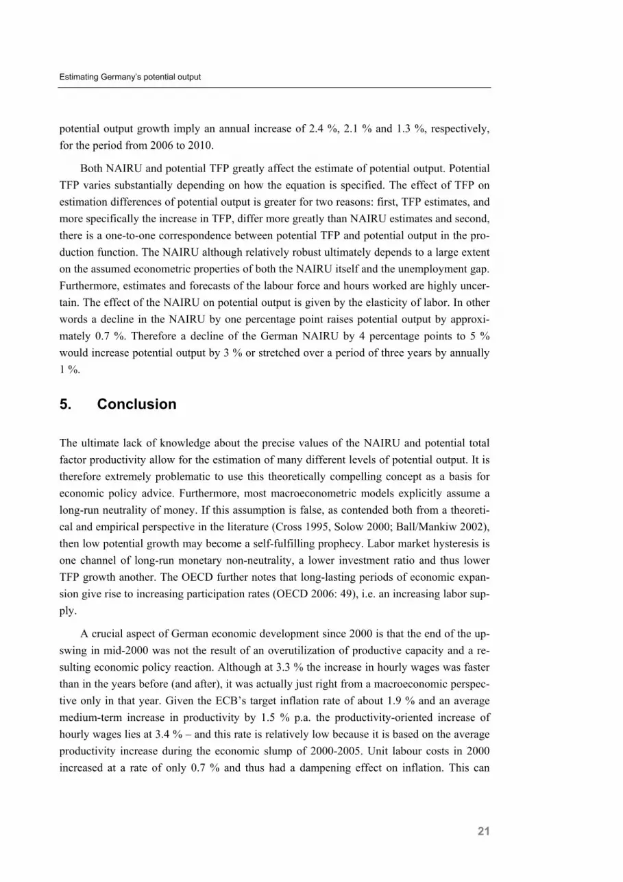
potential output growth imply an annual increase of 2.4 %, 2.1 % and 1.3 %, respectively, for the period from 2006 to 2010.

Both NAIRU and potential TFP greatly affect the estimate of potential output. Potential TFP varies substantially depending on how the equation is specified. The effect of TFP on estimation differences of potential output is greater for two reasons: first, TFP estimates, and more specifically the increase in TFP, differ more greatly than NAIRU estimates and second, there is a one-to-one correspondence between potential TFP and potential output in the pro-duction function. The NAIRU although relatively robust ultimately depends to a large extent on the assumed econometric properties of both the NAIRU itself and the unemployment gap. Furthermore, estimates and forecasts of the labour force and hours worked are highly uncer-tain. The effect of the NAIRU on potential output is given by the elasticity of labor. In other words a decline in the NAIRU by one percentage point raises potential output by approxi-mately 0.7 %. Therefore a decline of the German NAIRU by 4 percentage points to 5 % would increase potential output by 3 % or stretched over a period of three years by annually 1 %.

5. Conclusion

The ultimate lack of knowledge about the precise values of the NAIRU and potential total factor productivity allow for the estimation of many different levels of potential output. It is therefore extremely problematic to use this theoretically compelling concept as a basis for economic policy advice. Furthermore, most macroeconometric models explicitly assume a long-run neutrality of money. If this assumption is false, as contended both from a theoreti-cal and empirical perspective in the literature (Cross 1995, Solow 2000; Ball/Mankiw 2002), then low potential growth may become a self-fulfilling prophecy. Labor market hysteresis is one channel of long-run monetary non-neutrality, a lower investment ratio and thus lower TFP growth another. The OECD further notes that long-lasting periods of economic expan-sion give rise to increasing participation rates (OECD 2006: 49), i.e. an increasing labor sup-ply.

A crucial aspect of German economic development since 2000 is that the end of the up-swing in mid-2000 was not the result of an overutilization of productive capacity and a re-sulting economic policy reaction. Although at 3.3 % the increase in hourly wages was faster than in the years before (and after), it was actually just right from a macroeconomic perspec-tive only in that year. Given the ECB’s target inflation rate of about 1.9 % and an average medium-term increase in productivity by 1.5 % p.a. the productivity-oriented increase of hourly wages lies at 3.4 % – and this rate is relatively low because it is based on the average productivity increase during the economic slump of 2000-2005. Unit labour costs in 2000 increased at a rate of only 0.7 % and thus had a dampening effect on inflation. This can

21


hardly be interpreted as a sign of overheating.20 It follows that OECD and International Monetary Fund in spring of 2001 estimated the German output gap to be at -1.0 % and -0.9 %, respectively. In retrospect from the year 2006 the year 2000 is now interpreted to be a year of marked capacity overutilization: OECD and International Monetary Fund in retro-spect estimate the output gap to have been decidedly positive, at +1.8 % and +1.7 %, respec-tively. This drastically revised interpretation of the business cycle is not due to a reinterpreta-tion of the wage pressure or of the actual increase of GDP in 2000 and the years before, but rather to the methods used to estimate potential output. As discussed, these methods rely heavily on the most recent past. The economic weakness since 2000 has therefore led to a downward revision of potential output (growth). The main reason for the economic downturn was an inappropriate macroeconomic policy reaction to a series of adverse exogenous shocks since 2000.21 Had fiscal policy, in particular, reacted in an appropriate expansionary manner, German growth in 2001-2005 could have been significantly higher than the actual annual average of 0.6 % given an average increase in unit labour costs of only 0.1 % (Hein et al. 2005). Accordingly, unemployment rate and NAIRU would not have increased but rather fallen. The common methods of calculating potential output would have responded to higher growth by showing correspondingly higher potential growth rates.

Using the production function approach it is possible to identify factors that positively affect potential output, as for example, the investment ratio. But no estimate of potential output can be claimed to be accurate or precise and estimates for a given period vary signifi-cantly over time. This, however, vastly complicates fiscal planning and the use of monetary policy rules, such as the Taylor rule. Policy makers cannot rely on actual figures presented since they may change the following period. The bottom line is that potential output as measured by the methods presently available cannot be considered as a yardstick for eco-nomic policy theory.

In the literature there are three key proposals to deal with the uncertainty of potential output estimates. The first is based on Orphanides/Williams (2002) and argues that economic policy should be oriented towards GDP growth rates instead of the output gap (or changes in the unemployment rate rather than the unemployment gap). The second, closely related pro-posal recommends that economic policy makers quantify potential growth and thus the out-put gap conservatively, i.e. rather too small than too large (European Commission 2002: 9). Both proposals essentially imply that the status quo – the existing trend – is reinforced. Fur-thermore, both may provoke excessive policy reactions (Yellen 2002: 132f.). Focussing on the status quo and restrictive macro policy have even more serious implications if macro

20 The fact that inflation in Germany reached 2 % in 2001 was primarily the result of the drastic

oil price hike and the increase in food prices due to two animal diseases – unit labour costs rose by only 0.6 % in 2001 (Federal Statistical Office).

21 To be named first an foremost are the oil price shock and the international collapse of stock prices at the beginning of the decade, but also the US recession, the terror acts of 9/11 and the geopo-litical uncertainties relating to the war in Iraq as well as the further increase in oil prices well into the year 2006.

22


policy is not (super-) neutral in the long run but rather affects not only GDP but also poten-tial output, via hysteresis effects for example. Therefore we find the third proposal superior that argues for giving uncertain output gaps less weight in monetary policy decisions (Smets 1998, Meyer 2000 and Orphanides/Williams 2002). We argue, however, that whilst eco-nomic policy should disregard output gap estimates, it should nonetheless act preemtively by keeping a close eye on wage costs and, in particular, unit labour costs. Unit labour costs are a good indicator for underlying inflation which, in turn, provides information about the under- or overutilization of capacity (Fagan et al. 2001; Duong et al. 2005: 35). For fiscal policy the lack of reliable output gap estimates would be less problematic if its focus were on longer term expenditure paths rather than structural deficits (Horn/Truger 2005).

Given the difficulties involved in robustly estimating potential output, economic policy makers need to learn to pursue their policy objectives without reference to this variable. Pragmatism should prevail. In the face of a benign inflation outlook and high unemployment economic policy should strive to test the limits of potential output and to set in motion a virtuous cycle of a decreasing NAIRU, a rising participation rate, higher productivity growth and an improvement in fiscal balances.

23


6. Literature

Akerlof, G. A., Dickens, W. T. and Perry, G. L. (2000): Near-Rational Wage and Price Setting and the Long-Run Phillips Curve, Brookings Papers on Economic Activity 1, 1-60.

Apel, M. and Jansson, P. (1999): A Theory-Consistent System Approach for Estimating Po-tential Output and the NAIRU, Empirical Economics 24(3), 373-388.

Ball, L. (1999): Aggregate Demand and Long-run Unemployment, Brookings Papers on Eco-nomic Activity 2, 189-251.

Ball, L. (1999): Policy Rules for Open Economies. Ed. by J. Taylor. Monetary Policy Rules. London 1999.

Ball, L. and Mankiw, N. G. (2002): The NAIRU in Theory and Practice, Journal of Economic Perspectives 16(4), 115-136.

Barreto, H. and Howland, D. (1993): There Are Two Okun's Law Relationships Between Output and Unemployment, unveröffentlichten Papier des Wabash College.

Bassanini, A. and Duval, R. (2006): Employment Patterns in OECD Countries: reassessing the role of policies and institutions, OECD Social, Employment and Migration Working Paper 35, and OECD Economics Department Working Paper 486, Paris.

Bean, CH. R. (1997): The role of demand-management policies in reducing unemployment. Unemployment Policy. Government Options for the Labour market. Ed. by D. J. Snower and G. de la Dehesa. Centre for Economic Policy Research, Cambridge University Press, 83-111.

Bernanke, B. S. and Blinder, A. S. (1992): The Federal Funds Rate and the Channels of Monetary Transmission, American Economic Review 82(4), 901-21.

Blanchard, O. J and Wolfers, J. (2000): The Role of Shocks and Institutions in the Rise of European Unemployment: the Aggregate Evidence, The Economic Journal 110(462), C1-C33.

Blanchard, O. J. and Katz, L. F. (1997): What We Know and What We Do Not Know About the Natural Rate of Unemployment, Journal of Economic Perspectives 11(1), 51-72.

Blanchard, O. and L. H. Summers (1986): Hysteresis and the European Unemployment Problem. Working papers 427, Massachusetts Institute of Technology (MIT), Depart-ment of Economics.

Burda, M. and Ch. Wyplosz (1994): Makroökonomik. Eine europäische Perspektive. Vahlen, Munich.

Calmfors, L. and Driffill, J. (1988): Bargaining Structure, Corporatism and Macroeconomic Performance, Economic Policy 6, 14-61.

Carlin, W. and Soskice, D. (1990): Macroeconomics and the Wage Bargain - A Modern Ap-proach to Employment, Inflation, and the Exchange Rate, Oxford University Press, Ox-ford.

CBO – Congressional Budget Office (2006): The Budget and Economic Outlook: Fiscal Years 2007 to 2016, Table 2-2: Key Assumptions in CBO’s Projection of Potential Out-put. Januar, Washington DC.

Clarida, R. J., Galí, I. and Gertler, M. (1999): The Science of Monetary Policy: A New Keynesian Perspective, Journal of Economic Literature 37(4), 1661-1707.

Cross, R. (1995): Is the Natural Rate Hypothesis Consistent with Hysteresis?, The Natural Rate of Unemployment. Reflections in 25 years of the Hypothesis. Ed. by R. Cross, chap. 10, 181-200. Cambridge University Press, Cambridge.

Denis, C., McMorrow, K. und Röger, W. (2002): Production Function Approach To Calculat-ing Potential Growth And Output Gaps – Estimates For The EU Member States And The US, Economic Papers 176, European Commission.

Deutsche Bundesbank (1999): Taylor-Zins and Monetary Conditions Index, Monatsbericht April, 47-63.

24


Deutschen Bundesbank (2005): Monthly Bulletin, Juni. Döpke, J. (2004): Real-time data and business cycle analysis in Germany. Discussion Pa-

per, Studies of the Economic Research Centre 11/2004. Duong, M./Logeay, C./Stephan, S./Zwiener, R. with the collaboration of Serhiy Yahnych,

Modelling European Business Cycles (ECB Model), DIW Berlin, Data Documentation 5, 2005, Berlin

Espinosa-Vega, M. A. (1998): How powerful is monetary policy in the long run? Economic Review, Federal Reserve Bank of Atlanta, issue 3 Q, 12-31.

European Commission (2002): The EU economy: 2002 review. European Economy, No. 6. European Commission (2006): Public Finances in EMU 2006. Erscheint in Kürze in Europe-

an Economy 3/2006. Fagan, G./Henry, J./Mestre, R. (2001): An area-wide model (AWM) for the euro area, ECB

Working Paper Nr. 42, 2001, Frankfurt. Fabiani, S. and Mestre, R. (2000): Alternative measures of the NAIRU in the Euro Area: Es-

timates and assessment, ECB Working Paper 17. Fabiani, S. and Mestre, R. (2001): A System Approach for Measuring the Euro Area NAIRU,

ECB Working Paper 65. Filc, W. (2002): Überlegungen zum wachstumsneutralen Zins. Ed. by A. Heise, Neues Geld

– alte Geldpolitik? Die EZB im makroökonomischen Interaktionsraum, Marburg, Me-tropolis, 157-174.

Fitoussi, J. P., Jestaz, D., Phelps, E. S. and Zoega, G (2000): Roots of the Recent Recover-ies: Labor Reforms or Private Sector Forces? Brookings Papers on Economic Activity I, 237-311.

Gordon, R. J. (1997): The Time-Varying NAIRU and its Implications for Economic Policy, Journal of Economic Perspectives 11(1).

Greenwald, B. and Stiglitz, J. (1993): New and Old Keynesians, Journal of Economic Per-spectives 7(1), 23-44.

Harvey, A. C. and Jaeger, A. (1993): Detrending, stylized facts and the business cycle, Jour-nal of Applied Econometrics 8(3), 231-247.

Hein, E., Horn, G., Tober, S. und Truger, A. (2005): Eine gesamtwirtschaftliche Polit-Strategie für mehr Wachstum und Beschäftigung, WSI-Mitteilungen 8/2005.

Horn, G. und Truger, A. (2005): Strategien zur Konsolidierung der öffentlichen Haushalte, WSI-Mitteilungen 8/2005.

International Monetary Fund (2001): Estimating Potential Output and the NAIRU for the Euro Area. Monetary and Exchange Rate Policies of the Euro Area: Selected Issues, IMF Country Report 1, 4-15.

International Monetary Fund: World Economic Outlook, September, several spring issues. Jaeger, A. and Parkinson, M. (1994): Some evidence on hysteresis in unemployment rates,

European Economic Review 38(2), 329-342. Johansen, K. (1995): Norvegian Wage Curves, Oxford Bulletin of Economics and Statistics

52(2), 229-247. Kalecki, M. (1939): Essays in the Theory of Economic Fluctuations. London. Kalecki, M. (1942): A Theory of Profits, Economic Journal 52(206/7), 258-267. Keynes, J. M. [1936] (1964): The General Theory of Employment, Interest, and Money. San

Diego/New York/London. King, R. G. (2000): The New IS-LM Model: Language, Logic, and Limits, Federal Reserve

Bank of Richmond, Economic Quarterly 86(3). Layard, R., Nickell, S. and Jackman, R (1991): Macroeconomic Performance and the Labour

Market, Oxford University Press. Léon-Ledesma, M. A. (2002): Unemployment Hysteresis in the United States and the EU: A

Panel Approach, Bulletin of Economic Research 54(2), 95-103.

25


Léon-Ledesma, M. A. and McAdam, P. (2004): Unemployment, Hysteresis and Transition, Scottish Journal of Political Economy 51(3), 377-401.

Leijonhufvud, A. (1990): Nautral Rate and Market Rate, The New Palgrave. Money. Ed. by J. Eatwell, M. Milgate and P. Newman. Macmillan, London, Basingstoke, 268-272.

Logeay, C. and Tober, S. (2006): Hysteresis and the NAIRU in the Euro Area, Scottish Jour-nal of Political Economy 53(4), 409-429.

Logeay, C. and Tober, S. (2006): Real Interest Rates and the NAIRU in the Euro Area. Eu-rostat Proceedings, im Erscheinen.

Machin, S. and Manning, A. (1999): The Causes and Consequences on Longterm Unem-ployment in Europe, Handbook for Labour Economics. Ed. by O. C. Ashenfelter and D. Card, 3C, Chap. 47, 3085-3139, North-Holland.

Mankiw, N. G. (1985): Small Menu Costs and Large Business Cycles: A Macroeconomic Model of Monopoly. Quarterly Journal of Economics 100, 529-537. Neu abgedruckt in Mankiw and Romer 1 (1991).

Martinez-Mongay, C. (2000): ECFIN’s Effective tax rates. Properties and Comparisons with other tax indicators, Econonomic Papers 146.

Martinez-Mongay, C. (2003): Labour Taxation in the European Union. Convergence, Compe-tition, Insurance?, Konferenzbeitrag, Banca d’Italia Workshop on Tax Policy, 2-5. April 2003, Perugia.

McCallum, B. T. (2001): Should Monetary Policy Respond Strongly to Output Gaps?, Ameri-can Economic Review. Papers and Proceedings 91(2), 258-262.

Meyer, L. H. (2000): Structural Change and Monetary Policy. Remarks Before the Joint Con-ference of the Federal Reserve Bank of San Francisco and the Stanford Institute for Economic Policy Research, Federal Reserve Bank of San Francisco, San Francisco, California March 3, 2000.

Modigliani, F. and Papademos, L. (1975): Targets for Monetary Policy in the coming year. Brookings Paper on Economic Activity I, 141-163.

Nickell, S. Nunziata, L., Ochel, W., Quintini, G. (2001): The Beveridge Curve, Unemployment and Wages in the OECD from the 1960s to the 1990s - Preliminary Version. CEP-Working Paper 502.

Nickell, S. Nunziata, L., Ochel, W., Quintini, G. (2001): The Beveridge Curve, Unemployment and Wages in the OECD from the 1960s to the 1990s - Preliminary Version. CEP-Working Paper 502.

Nickell, S., Nunziata, L., Ochel,W. and Quintini, G. (2002): The Beveridge curve, unemploy-ment and wages in the OECD from the 1960s to the 1990s. Ed. by P. Aghion, R. Frydman, J. Stiglitz and M. Woodford. Knowledge, Information, and Expectations in Modern Macroeconomics: In Honour of Edmund S. Phelps, Princeton University Press, Princeton, Kap. 19, 394–440.

OECD: Economic Outlook, Paris, several spring issues. OECD (2006): Employment Outlook – Boosting Jobs and Income, June Okun, A. M. (1962): Potential GNP: Its measurement and its significance. Proceedings of the

Business and Economic Statistics Section, American Statistical Association, 98-103. Orphanides, A. (1998): Monetary Policy Evaluation with Noisy Information, Finance and

Economics Discussion Series No.1998: 50. Washington, D.C.: Board of Governors of the Federal Reserve System, November 1998.

Orphanides, A. und Williams J. C. (2002): Robust Monetary Policy Rules with Unknown Natural Rates. Brookings Papers on Economic Activity 2/2002, 63-126.

Patinkin, D. (1992): Real Balances. The New Palgrave Dictionary of Money and Finance. Hrsg. von P. Newman, M. Milgate and J. Eatwell. Macmillan, London, Vol. 3, 295-298.

Planas, Ch., Roeger, W. and Rossi A. (2006): How much has labour taxation contributed to European structural unemployment? Erscheint demnächst in Journal of Economic Dy-namics and Control.

26


Riese, H. (1986): Theorie der Inflation. Tübingen. Robinson J. (1962): Economic Philosophy. Penguin Books. Røed, K. (1997): Hysteresis in Unemployment, Journal of Economic Surveys 11(4), 389-418. Salemi, M. K. (1999): Estimating the Natural Rate of Unemployment and Testing the Natural

Rate Hypothesis, Journal of Applied Econometrics 14(1), 1-25. Smets, F. (1998): Output Gap Uncertainty: Does it matter for the Taylor rule? BIS Working

Papers, No. 60 – November 1998. Solow, R. M. (1998): How cautious must the Fed be? Inflation, Unemployment, and Mone-

tary Policy. Ed. by B. M. Friedman, S. 1-28. The MIT Press, Cambridge, USA. Solow, R. M. (2000): Unemployment in the United States and in Europe: A contrast and the

reasons, Working Paper 231, CESifo. Spahn, H.-P. (1997): Disinflation and Arbeitslosigkeit. Über die Nichtneutralität der Geldpoli-

tik. Diskussionsbeiträge aus dem Institut für Volkswirtschaftslehre (520), Universität Ho-henheim.

Tobin, J. (1980): Stabilization Policy Ten Years After, Brookings Papers on Economic Activ-ity 1, 19-71.

Tobin, J. (1993): Price Flexibility and Output Stability: An Old Keynesian View, Journal of Economic Perspectives 7(1), 45-65.

Turner, D., Boone, L., Giorno, C., Meacci, M., Rae, D. und Richardson, P. (2001): Estimating the structural rate of unemployment for the OECD countries, OECD Economic Studies II(33),171-216.

Visser, J. (2006): Union Membership statistics in 24 countries, Monthly Labor review, Jan., 38-49.

Wicksell, K. (1936): Interest and Prices (Übersetzung der 1898er Ausgabe von R.F. Kahn). London: Macmillan.

Yellen, J. L. (2002): Comments. Brookings Papers on Economic Activity 2/2002, 126-135.

27

Publisher: Hans-Böckler-Stiftung, Hans-Böckler-Str. 39, 40476 Düsseldorf, Germany Phone: +49-211-7778-331, [email protected], http://www.imk-boeckler.de IMK Working Paper is an online publication series available at: http://www.boeckler.de/cps/rde/xchg/hbs/hs.xls/31939.html ISSN: 1861-2199 The views expressed in this paper do not necessarily reflect those of the IMK or the Hans-Böckler-Foundation. All rights reserved. Reproduction for educational and non-commercial purposes is permitted provided that the source is acknowledged.

mailto:[email protected]

http://www.imk-boeckler.de/

Documents

Estimating Germany's Potential Output