Estimating the Potential Economic Value of Seasonal Forecasts in West Africa: A Long-Term Ex-Ante Assessment in Senegal

Estimating the Potential Economic Value of Seasonal Forecasts in West Africa:A Long-Term Ex-Ante Assessment in Senegal

BENJAMIN SULTAN

IRD, LOCEAN/IPSL, Laboratoire d’Oceanographie et du Climat: Experimentation et Approche Numerique,

UMR 7159 (CNRS/IRD/UPMC/MNHN), Universite Pierre et Marie Curie, Paris, France

BRUNO BARBIER

CIRAD, UMR G-EAU/2iE, Ouagadougou, Burkina Faso

JEANNE FORTILUS

IRD, LOCEAN/IPSL, Laboratoire d’Oceanographie et du Climat: Experimentation et Approche Numerique,

UMR 7159 (CNRS/IRD/UPMC/MNHN), Universite Pierre et Marie Curie, Paris, France

SERIGNE MODOU MBAYE

ANCAR, Nioro du Rip, Senegal

GREGOIRE LECLERC

CIRAD, UR GREEN, LERG, Ecole Superieure Polytechnique, Universite Cheikh Anta Diop, Dakar, Senegal

(Manuscript received 27 April 2009, in final form 29 September 2009)

ABSTRACT

Recent improvements in the capability of statistical or dynamic models to predict climate fluctuations

several months in advance may be an opportunity to improve the management of climatic risk in rain-fed

agriculture. The aim of this paper is to evaluate the potential benefits that seasonal climate predictions can

bring to farmers in West Africa. The authorAU1 s have developed an archetypal bioeconomic model of a small-

holder farm in Nioro du Rip, a semiarid region of Senegal. The model is used to simulate the decisions of

farmers who have access to a priori information on the quality of the next rainy season. First, the potential

economic benefits of a perfect rainfall prediction scheme are evaluated, showing how these benefits are af-

fected by forecast accuracy. Then, the potential benefits of several widely used rainfall prediction schemes are

evaluated: one group of schemes based on the statistical relationship between rainfall and sea surface tem-

peratures, and one group based on the predictions of coupled ocean–atmosphere models.

The results show that forecasting a dryer than average rainy season would be the most useful to Nioro du

Rip farmers if they interpret forecasts as deterministic. Indeed, because forecasts are imperfect, predicting

a wetter than average rainy season exposes the farmers to a high risk of failure by favoring cash crops such as

maize and peanut that are highly vulnerable to drought. On the other hand, the farmers’ response to a forecast

of a dryer than average rainy season minimizes the climate risk by favoring robust crops such as millet and

sorghum, which will tolerate higher rainfall in case the forecast is wrong.

When either statistical or dynamic climate models are used for forecasting under the same lead time and the

same 31-yr hindcast period (i.e., 1970–2000), similar skill and economic values at farm level are found. When

a dryer than average rainy season is predicted, both methods yield an increase of the farmers’ income—13.8%

for the statistical model and 9.6% for the bias-corrected Development of a European Multimodel Ensemble

Prediction System for Seasonal to Interannual Prediction (DEMETER) multimodel ensemble mean.

wcas1022

Corresponding author address: Benjamin Sultan, UMR 7159 (CNRS/IRD/UPMC/MNHN), Universite Pierre et Marie Curie, Case 100,

4 Place Jussieu, 75252 Paris, CEDEX 05, France.

E-mail: [email protected]

JOBNAME: WCAS 00#0 2009 PAGE: 1 SESS: 8 OUTPUT: Thu Dec 3 15:34:47 2009 Total No. of Pages: 19/ams/wcas/0/wcas1022

MONTH 2009 S U L T A N E T A L . 1

DOI: 10.1175/2009WCAS1022.1

� 2009 American Meteorological Society

Wea

ther

, Clim

ate,

and

Soc

iety

(Pro

of O

nly)

1. Introduction

Climate has a strong influence on agricultural pro-

duction, is considered to be the most weather dependent

of all human activities (Oram 1989; Hansen 2002), and it

has socioeconomic impacts whose magnitude varies

greatly from one region to another (Ogallo et al. 2000).

The severity of climate impacts is particularly strong in

the Sahel, where rain-fed agriculture is the main source

of food and income and where the means to control the

crop environment (irrigation, mechanization, fertilizers,

and other off-farm inputs) are largely unavailable to

small-scale farmers (Ingram et al. 2002). Dealing with

the uncertainty of climate variability is a challenge for

agriculture as farmers need to make critical climate-

sensitive decisions months before the actual rainy sea-

son takes place (Meza et al. 2008). Therefore, forecasts

about future climate might help African farmers take

crucial strategic decisions to reduce their vulnerability

and increase farm profitability.

Good predictability of seasonal climate fluctuations

has been achieved for many parts of the world (Hansen

2002) by using comprehensive coupled models of the

atmosphere, oceans, and land surface (Palmer et al. 2004)

or regional statistical schemes (Ward 1998; Fontaine et al.

1999; Ogallo et al. 2000; Ward et al. 2004). In addition,

the general circulation models are now able to produce

plausible long-run climate change scenarios in response

to various evolutions of greenhouse gas concentrations.

Improved climate prediction capability might provide

an opportunity for farmers to adapt their current man-

agement to a highly variable present climate (Ingram

et al. 2002) as well as to future climate change (Lobell

et al. 2008). However, obtaining these potential benefits

is not straightforward because forecasting is imperfect

and its application to management issues has not been

developed and tested extensively (Hammer et al. 2001).

Meza et al. (2008) provide an exhaustive review of such

approaches assessing the economic value of seasonal

forecasts. Here, the authors distinguish ex-ante evalua-

tion (i.e., assessing the benefits of forecasts in advance

of their adoption by society) from ex-post evaluation,

which seeks to assess observed outcomes following

adoption of actual forecast schemes. Even if seasonal

forecasts are made routinely in sub-Saharan Africa (as

in other parts of the world), adoption by farmers is too

low to provide any reliable ex-post evaluation (Meza

et al. 2008; Roncoli et al. 2000). Ex-ante approaches

remain the best way to evaluate the forecasts, and they

also present several advantages. They provide quanti-

tative arguments which are often necessary to mobilize

funds and institutional partners and to focus on where

the benefits are likely to be the greatest (Thornton 2006;

Meza et al. 2008). The review of Meza et al. (2008) pres-

ents 58 assessments of the economic value of seasonal

forecasts for agriculture based on 33 scientific papers.

However, none of the referenced studies considers sub-

Saharan Africa or even subsistence agriculture. This

paper is an attempt to fill this gap.

The aim of the present study is (i) to develop a meth-

odology to assess the usefulness of seasonal forecasts in

West Africa, by taking into account both climatic and

economic evaluations, and (ii) to apply this methodology

to state-of-the-art climate predictions that are or can be

made routinely in the subcontinent. To be consistent with

the existing categorical climate prediction systems in West

Africa (Previsions Climatiques Saisonnieres en Afrique

de l’Ouest, le Tchad et le Cameroun, PRESAO; see http://

www.acmad.ne; Hamatan et al. 2004; Ward et al. 2004), we

will focus on forecasts of total seasonal (July to Septem-

ber) rainfall amount categories according to the terciles of

the expected distribution of values: wet (upper tercile),

normal (middle tercile), and dry (lower tercile). How-

ever, although PRESA AU2O and major forecasting centers

provide probabilistic information (e.g., as probability

shifts of the climatological tercile categories), this study

will mostly examine the deterministic case (i.e., farmers

supposing the next rainy season will be in the most

probable tercile category). This allows us to document

which management changes would be needed with a

perfect knowledge of the coming rainy season to opti-

mize farmers’ income and what would be the economic

value of these changes. We thus refer to the potential

economic value since we take into account neither the

probabilistic nature of forecasts nor dissemination, ac-

ceptation, and adoption of forecast within local knowl-

edge frameworks, which would define the real economic

value of the forecasts. Moreover, we understand that

forecasting total rainfall is of limited usefulness for

farmers since it is the timing of the onset and end of the

rainy season and the distribution of rainfall within the

season that are the more salient parameters that may in-

fluence farmers’ cropping decisions (Ingram et al. 2002).

For our purpose, we developed a simple bioeconomic

farm model based on a typical smallholder farm in the

Sahelian zone of Senegal. This kind of model has already

been used to estimate the value of forecast information

(Wilks 1997). While farm-level models can be enhanced

to take into account climatic risk (Cocks 1968; Hazell

and Norton 1986), we prefer, like Cabrera et al. (2006),

to estimate risk by running simulations with actual cli-

mate data. The model, described in section 2, is used to

simulate the farmers’ response to the adoption of cate-

gorical forecast. By looking at the differences between

the simulated farmers’ income with and without a priori

information on probable future rainfall amounts, it is

2 W E A T H E R , C L I M A T E , A N D S O C I E T Y VOLUME 00


Wea

ther

, Clim

ate,

and

Soc

iety

(Pro

of O

nly)

https://www.researchgate.net/publication/234007969_Development_of_a_European_Multi-Model_Ensemble_System_for_Seasonal_to_Interannual_Prediction_DEMETER?el=1_x_8&enrichId=rgreq-4e1a0333-04fa-4950-b8f9-b91b3d49ca5a&enrichSource=Y292ZXJQYWdlOzI0MDY4OTI5MztBUzoxOTk2ODgzNzc2Mzg5MTJAMTQyNDYyMDgyNzE1NQ==

https://www.researchgate.net/publication/4748759_Opportunities_and_constraints_for_farmers_of_West_Africa_to_use_seasonal_precipitation_forecasts_with_Burkina_Faso_as_a_case_study_Agr_Syst?el=1_x_8&enrichId=rgreq-4e1a0333-04fa-4950-b8f9-b91b3d49ca5a&enrichSource=Y292ZXJQYWdlOzI0MDY4OTI5MztBUzoxOTk2ODgzNzc2Mzg5MTJAMTQyNDYyMDgyNzE1NQ==


https://www.researchgate.net/publication/228715987_Applications_of_seasonal_to_interannual_climate_to_agricultural_planning_and_operations?el=1_x_8&enrichId=rgreq-4e1a0333-04fa-4950-b8f9-b91b3d49ca5a&enrichSource=Y292ZXJQYWdlOzI0MDY4OTI5MztBUzoxOTk2ODgzNzc2Mzg5MTJAMTQyNDYyMDgyNzE1NQ==

https://www.researchgate.net/publication/222657352_Realizing_the_potential_benefits_of_climate_prediction_to_agriculture_issues_approaches_challenges_Agr_Syst?el=1_x_8&enrichId=rgreq-4e1a0333-04fa-4950-b8f9-b91b3d49ca5a&enrichSource=Y292ZXJQYWdlOzI0MDY4OTI5MztBUzoxOTk2ODgzNzc2Mzg5MTJAMTQyNDYyMDgyNzE1NQ==

https://www.researchgate.net/publication/237334755_Impact_of_climate_information_on_reducing_farm_risk_by_optimizing_crop_insurance_strategy?el=1_x_8&enrichId=rgreq-4e1a0333-04fa-4950-b8f9-b91b3d49ca5a&enrichSource=Y292ZXJQYWdlOzI0MDY4OTI5MztBUzoxOTk2ODgzNzc2Mzg5MTJAMTQyNDYyMDgyNzE1NQ==

https://www.researchgate.net/publication/4731030_Advances_in_application_of_climate_prediction_in_agriculture_Agr_Syst?el=1_x_8&enrichId=rgreq-4e1a0333-04fa-4950-b8f9-b91b3d49ca5a&enrichSource=Y292ZXJQYWdlOzI0MDY4OTI5MztBUzoxOTk2ODgzNzc2Mzg5MTJAMTQyNDYyMDgyNzE1NQ==

https://www.researchgate.net/publication/227244655_Sensitivity_of_agricultural_production_to_climatic_change?el=1_x_8&enrichId=rgreq-4e1a0333-04fa-4950-b8f9-b91b3d49ca5a&enrichSource=Y292ZXJQYWdlOzI0MDY4OTI5MztBUzoxOTk2ODgzNzc2Mzg5MTJAMTQyNDYyMDgyNzE1NQ==

https://www.researchgate.net/publication/235669340_Economic_Value_of_Seasonal_Climate_Forecasts_for_Agriculture_Review_of_Ex-Ante_Assessments_and_Recommendations_for_Future_Research?el=1_x_8&enrichId=rgreq-4e1a0333-04fa-4950-b8f9-b91b3d49ca5a&enrichSource=Y292ZXJQYWdlOzI0MDY4OTI5MztBUzoxOTk2ODgzNzc2Mzg5MTJAMTQyNDYyMDgyNzE1NQ==



possible to evaluate quantitatively the value of that kind

of climate forecast.

By solving the farm model we obtain the farmer’s dif-

ferent optimal management strategies in response to the

use of a forecast, as well as his resulting income. This allows

us to make an ex-ante assessment of the economic value of

the forecasts and its sensitivity to the forecast accuracy (or

skill). Finally, we evaluate two state-of-the-art climate

prediction methods: a statistical forecast based on the well-

documented link between rainfall and sea surface tem-

perature (SST) and a dynamical forecast system based on

the outputs of seven comprehensive European global

coupled atmosphere–ocean models from the Development

of a European Multimodel Ensemble Prediction System

for Seasonal to Interannual Prediction (DEMETER)

project (Palmer et al. 2004). This evaluation is done over

a 31-year hindcast period from 1970 to 2000.

2. Materials and methods

a. Rainfall data in Senegal

Mitchell and Jones (2005) have produced a global cli-

mate observations database including 1224 monthly grids

of observed climate for the period 1901–2002 and covering

the global land surface at 0.58 resolution. This database is

known as the Climatic Research Unit (CRU) TS 2.1 and is

publicly available (http://www.cru.uea.ac.uk/cru/data/hrg/

cru_ts_2.10). There are nine climate variables available:

daily mean, minimum and maximum temperature, diurnal

temperature range, precipitation, wet day frequency, frost

day frequency, vapor pressure, and cloud cover. In this

study, we use rainfall data for the period 1970–2000. We

compute a Senegal rainfall index by averaging rainfall

data over the grid points from 11.58 to 168N in latitude and

168 to 11.58W in longitude and computing the mean July–

September (JAS) rainfall amount (mm month21). The

Nioro du Rip region, where the bioeconomic model has

been calibrated, is located near the center of the Senegal

rainfall index domain (F F1ig. 1). The area covered by the

rainfall index is much larger than the Nioro du Rip region

since the choice of the domain size is motivated by the

spatial resolution of the climate models’ predictions (see

section 2c). However, when averaging JAS rainfall, there

is good agreement between the large scale of the index

and the farm scale. This agreement is assessed by com-

paring the CRU data and nine local rainfall stations lo-

cated at Nioro du Rip with 31 years of data. We first

transform the Senegal rainfall index from CRU data into

FIG. 1. Map of the studied area in Senegal. The area delimited by the thick black line represents the Nioro du Rip

department where the bioeconomic model was calibrated. The thick gray box represents the area for which rainfall

indexes were computed. The thin grid corresponds to the 2.58 DEMETER model outputs.



Wea

ther

, Clim

ate,

and

Soc

iety

(Pro

of O

nly)


binary time series in which only three outcomes are pos-

sible: an occurrence of a ‘‘wet,’’ ‘‘normal,’’ or ‘‘dry’’ year,

according to whether the rainfall of the year is above the

upper tercile, between the upper and the lower tercile, or

below the lower tercile of the 31-yr rainfall distribution.

Since the JAS Senegal rainfall data are normally distrib-

uted, it permits classification of the years according to

tercile groups that divide the sorted dataset into three

equal parts so that each part represents 1/3 of the sampled

population. For each category defined from CRU data, we

look at the fraction of wet, normal, and dry situations de-

picted from local data from 279 situations (31 years and 9

locations in Nioro du Rip). FF2 igure 2 shows that a dry (wet)

year depicted by the Senegal index from CRU data cor-

responds to a dry (wet) or a normal situation in about 90%

of the cases and corresponds to a strictly dry (wet) situa-

tion in around 60% of the cases. The normal year as de-

picted from the Senegal rainfall index is less discriminate

at the local scale because it corresponds to a normal sit-

uation in only 40% of the cases.

b. Seasonal rainfall hindcasts

1) STATISTICAL TECHNIQUES

A number of empirical studies have been made using

prerainy season SST to predict the summer Sahelian

rainfall total (Folland et al. 1991; Ward 1998; Ward et al.

2004), which helped us in building our own simple sta-

tistical model to predict Senegal total summer rainfall.

This model is based on SST data from the monthly ex-

tended reconstructed sea surface temperature (ERSST;

see http://www.ncdc.noaa.gov/oa/climate/research/sst/

ersstv3.php), which is built using the most recently SST

data available from the International Comprehensive

Ocean–Atmosphere Dataset (ICOADS) and improved

statistical methods that allow stable reconstruction using

sparse data (Smith et al. 2008). Only the SST data over the

1970–2000 period are used in this study. We first compute

lagged correlation maps between the JAS Senegal rainfall

and SST in each of April, May, and June (F F3ig. 3). First,

there is a positive correlation between tropical Atlantic

SST and West Sahel rainfall, implying that wetter years

are associated with warmer SST in this basin through

a northward migration of the intertropical convergence

zone over the tropics. Second, West Sahel rainfall has

a strong connection with Pacific SST in which a warm

phase of El Nino–Southern Oscillation is associated with

reduced precipitation in the Sahel (Janicot et al. 2001).

The correlation maps are then used to select a set of

predictors that are box averages of SST over specific

regions known to be linked with the West African mon-

soon (Ward 1998; Giannini et al. 2003), where the highest

significant correlations are found (Fig. 3). Three sets of

predictors are selected independently, corresponding to

the three considered months. These predictors are then

used to build a stepwise multivariate linear regression

model to predict the JAS Senegal rainfall. The equation

of the multivariate model is

Y 5 a 1 b1X

11 � � � 1 b

pX

p,

where Y represents the predicted JAS Senegal rainfall

value, a is a constant, and each b term denotes a regres-

sion coefficient for the corresponding SST predictor X for

FIG. 2. Comparison between the Senegal rainfall index based on CRU TS 2.1 data (Mitchell

and Jones 2005) and local data. The sample of local data is composed of 279 situations (31 years

and 9 locations in Nioro du Rip). For each category—dry, normal, and wet years defined from

CRU data—the figure shows the corresponding fraction (%) of wet (black), normal (dark

gray), and dry (light gray) situations depicted from local data.



Wea

ther

, Clim

ate,

and

Soc

iety

(Pro

of O

nly)

https://www.researchgate.net/publication/9056687_Oceanic_Forcing_of_Sahel_Rainfall_on_Interdecadal_Time_Scales?el=1_x_8&enrichId=rgreq-4e1a0333-04fa-4950-b8f9-b91b3d49ca5a&enrichSource=Y292ZXJQYWdlOzI0MDY4OTI5MztBUzoxOTk2ODgzNzc2Mzg5MTJAMTQyNDYyMDgyNzE1NQ==

https://www.researchgate.net/publication/249610103_Diagnosis_and_Short-Lead_Time_Prediction_of_Summer_Rainfall_in_Tropical_North_Africa_at_Interannual_and_Multidecadal_Timescales?el=1_x_8&enrichId=rgreq-4e1a0333-04fa-4950-b8f9-b91b3d49ca5a&enrichSource=Y292ZXJQYWdlOzI0MDY4OTI5MztBUzoxOTk2ODgzNzc2Mzg5MTJAMTQyNDYyMDgyNzE1NQ==

https://www.researchgate.net/publication/225722741_Summer_Sahel-ENSO_teleconnection_and_decadal_time_scale_SST_variations?el=1_x_8&enrichId=rgreq-4e1a0333-04fa-4950-b8f9-b91b3d49ca5a&enrichSource=Y292ZXJQYWdlOzI0MDY4OTI5MztBUzoxOTk2ODgzNzc2Mzg5MTJAMTQyNDYyMDgyNzE1NQ==

https://www.researchgate.net/publication/248381934_Improvements_to_NOAA's_Historical_Merged_Land-Ocean_Surface_Temperature_Analysis_1880-2006?el=1_x_8&enrichId=rgreq-4e1a0333-04fa-4950-b8f9-b91b3d49ca5a&enrichSource=Y292ZXJQYWdlOzI0MDY4OTI5MztBUzoxOTk2ODgzNzc2Mzg5MTJAMTQyNDYyMDgyNzE1NQ==

FIG. 3. Correlations between JAS rainfall in Senegal and SST in (top) April, (middle) May,

and (bottom) June. The black boxes indicate the regions where SST was averaged to be in-

cluded in a statistical predictive model of JAS Senegal rainfall.



Wea

ther

, Clim

ate,

and

Soc

iety

(Pro

of O

nly)

a given month. Once a first model is built with all pre-

dictors, we reduce the number of predictors by mini-

mizing the variance inflation factor to reduce colinearity

among predictors in the model. In the same way, we also

apply ascendant and descendant methods to choose the

best set of predictors among the initial set. We built

three different models by using separately the April,

May, and June sets of predictors to explore three differ-

ent prediction lags where 30 April, 31 May, and 30 June

are the last days of observed data of the April, May, and

June models, respectively.

2) THE DEMETER HINDCASTS

Seasonal forecasts were also computed from the

DEMETER project (Palmer et al. 2004), whose objec-

tive was to develop a well-validated European coupled

multimodel ensemble forecast system for seasonal to

interannual prediction. The use of a multimodel en-

semble system based on seven comprehensive European

global coupled atmosphere–ocean models allows for

uncertainties in model formulation to be included in

the estimation of seasonal forecast probabilities and is

thought to produce the most reliable seasonal climate

forecasts possible. By the end of the project, an exten-

sive set of 6-monthly hindcast ensemble integrations had

been generated using the DEMETER system. These

were run four times a year starting on the first of Feb-

ruary, May, August, and November over a period of

about 40 years. Each model produced nine members of

the multimodel ensemble corresponding to nine differ-

ent ocean initial states (see Palmer et al. 2004). In this

study, we obtained hindcasts of monthly rainfall from

the online data retrieval system installed at the Eu-

ropean Centre for Medium-Range Weather Forecasts

(ECMWF; see http://www.ecmwf.int/research/demeter/

data/index.html) from 1970 to 2000 (TT1 able 1). We select

the integration starting on the first of May, which gives

a JAS rainfall prediction with the same lag as the April

statistical model [see section 2b(1)]. The outputs are

provided at 2.58 3 2.58 resolution. We compute the same

JAS Senegal rainfall index as for observation data

(section 2a), but for DEMETER hindcasts it is done by

(i) averaging the 63 model outputs (seven models and

nine initial ocean states) from June to September over

the 11.58–168N, 168–11.58W domain, (ii) computing the

seven individual model ensemble means by averaging

separately the nine runs of each model, and (iii) com-

puting the multimodel ensemble mean (MMEM) by

averaging the seven individual model ensemble means.

c. The climate evaluation

The forecast skill of the hindcasts was assessed using

two standard methods: (i) the correlation between ob-

servations and predictions by cross-validation and (ii) the

relative operating characteristics (ROC) scores.

The leave-one-out cross-validation method (Michaelsen

1987; Wilks et al. 2006) was used to document the stability

of the statistical SST models: model parameters were

computed from a portion of the data (called the training

period) composed by all years minus one, and we looked

at the prediction of the remaining data not used for

training. The cross-validated correlation is a realistic rep-

resentation of the skill of the model for ‘‘unseen’’ years.

Particularly adapted to small datasets, it partly reduces

distortion in skill estimates and protects against over-

fitting (Bouali et al. 2008 AU3). For DEMETER hindcasts we

computed a simple Pearson correlation coefficient be-

tween DEMETER rainfall outputs and the observed

JAS Senegal rainfall.

ROC is a mean of testing the skill of categorical

forecasts (Mason and Graham 1999; WMO 2006). It is

based on contingency tables giving the hit rate (HR) and

false alarm rate (FAR). To be consistent with actual

forecast schemes in West Africa, we first transform our

data and forecasts according to the terciles. We then

compute a contingency table based on these three cat-

egories and calculate the HR and FAR, which are sim-

ply percentages that tell us how well the forecast did

when a wet, normal, or dry year was observed and,

likewise, how well the forecast did when a wet, normal,

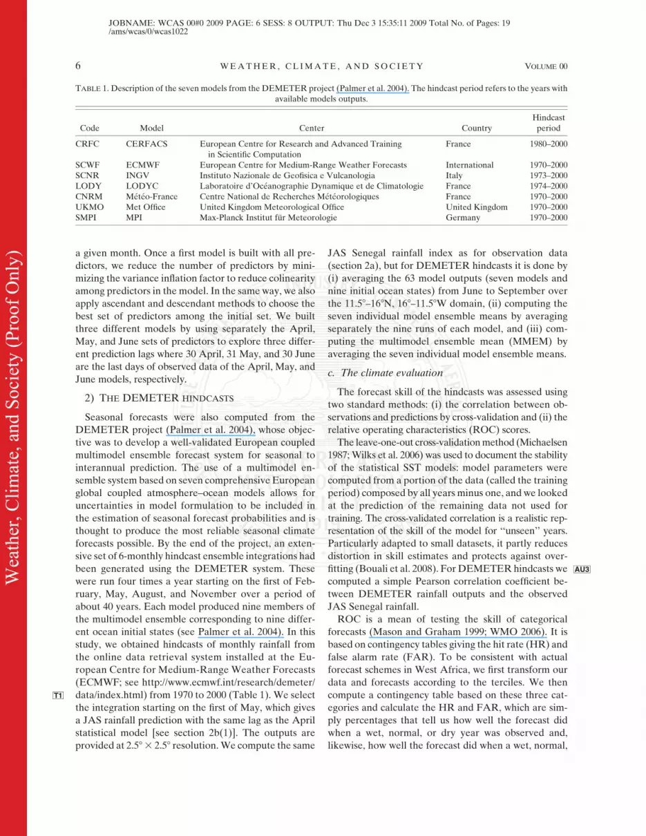
TABLE 1. Description of the seven models from the DEMETER project (Palmer et al. 2004). The hindcast period refers to the years with

available models outputs.

Code Model Center Country

Hindcast

period

CRFC CERFACS European Centre for Research and Advanced Training

in Scientific Computation

France 1980–2000

SCWF ECMWF European Centre for Medium-Range Weather Forecasts International 1970–2000

SCNR INGV Instituto Nazionale de Geofisica e Vulcanologia Italy 1973–2000

LODY LODYC Laboratoire d’Oceanographie Dynamique et de Climatologie France 1974–2000

CNRM Meteo-France Centre National de Recherches Meteorologiques France 1970–2000

UKMO Met Office United Kingdom Meteorological Office United Kingdom 1970–2000

SMPI MPI Max-Planck Institut fur Meteorologie Germany 1970–2000



Wea

ther

, Clim

ate,

and

Soc

iety

(Pro

of O

nly)




https://www.researchgate.net/publication/253913637_Conditional_Probabilities_Relative_Operating_Characteristics_and_Relative_Operating_Levels?el=1_x_8&enrichId=rgreq-4e1a0333-04fa-4950-b8f9-b91b3d49ca5a&enrichSource=Y292ZXJQYWdlOzI0MDY4OTI5MztBUzoxOTk2ODgzNzc2Mzg5MTJAMTQyNDYyMDgyNzE1NQ==

or dry year was not observed. An illustration of how the

contingency table is used, in the case when we are in-

terested in predicting wet years, is given in TT2 able 2. The

‘‘hits’’ category represents the number of wet years that

have been forecasted as such. The ‘‘false alarms’’ cate-

gory represents the number of nonwet years that have

been forecasted as wet years. The HR for the prediction

of wet years is defined as

HR 5hits

hits 1 misses.

It ranges between 0 and 1, 1 meaning that all occurrences

of wet years were correctly forecast as so. The FAR is

defined as

FAR 5false alarms

hits 1 false alarms.

The value can range between 0 and 1, 0 meaning that all

forecasted wet years were observed as so. The ROC score

is a measure of the hit rate to the false alarm rate. It is

recognized that the ROC score as applied to deterministic

forecasts is equivalent to the scaled Hanssen and Kuipers

score (HKS; WMO 2006AU4 ), which is defined as

HKS 5HR� FAR 1 1

2.

The range of possible values goes from 0 to 1; a perfect

forecast system has a value of 1 and a forecast system

with no information has an value of 0.5 (HR being equal

to FAR). The same skill scores can be computed for the

prediction of normal or dry years.

In our study, these standard forecast skill methods are

also applied to a reference forecast method based on

persistence (the JAS rainfall of one year belongs to the

same tercile as the previous year). Indeed, it has been

noticed by Ingram et al. (2002) that most farmers in

Burkina Faso make decisions about planting based on

what happened during the previous season.

d. The bioeconomic model

We designed a simple bioeconomic model based on

mathematical programming model of a typical farm in

Nioro du Rip in central Senegal using the General Al-

gebraic Modeling System (GAMS) software. The region

is under a semiarid climate regime and gets around

700 mm yr21 of rainfall in one short rainy season. With

more than 100 inhabitants per square kilometer, the

Nioro du Rip area experiences high population pressure.

New land is scarce and fallow has almost disappeared.

The cropping intensity over arable land is close to 1 but

agriculture remains of low intensity and is part of a het-

erogeneous landscape. Inputs are expensive, organic

matter application is rare, and crop yields remain low.

The use of animal traction with horses or donkeys is

widespread. Under the Food and Agriculture Organi-

zation (FAO)–United Nations Educational Scientific

and Cultural Organization (UNESCO) soil classifica-

tion system, Nioro du Rip soils were classified as pre-

dominantly dystric nitosols, tropical ferruginous soils

with various degrees of leaching. Farmers—who usually

make a good connection between the extremely variable

soil texture and expected yields—distinguish three types

of soils: lowlands, clayish soils (called deck locally), and

clayish soils with organic matter and sandy soils (called

dior). Farmers perceive important differences in yields

depending on the soil types cropped. Sandy soils are

easy to till but are permeable, making crops sensitive to

dry spells. They cover 38% of the province and support

mainly millet and peanut. Clayish soils (38% of the

province) are richer in micronutrients and organic mat-

ter but harder to till. They are more suited to maize and

sorghum. Mixed soils (deck dior) cover 10% of the area

and are suitable for most crops. Lithosols, which cover

6% of the area, are generally under pasture. Lowlands

(6% of the area) are suitable for rice, sorghum, and

vegetables during the dry season. Saline soils (3% of the

area) are unsuitable for agriculture. Overall, the major

crops are peanut and millet. However, maize area is

increasing fast because of a perceived recent increase of

rainfall, new policy incentives, and the increasing use of

fertilizers. Rice and sorghum are limited to lowlands.

The aim of the farm model is to find the conditions that

maximize the farmers’ global net income generated by

cropping activities for various types of rainy seasons

weighted by the probability of the occurrence of each

type of rainy season (i.e., wet, average, and dry). At this

stage, it is important to keep in mind that such a simple

model is not designed to help farmers, agricultural ex-

tension agents, or even decision makers directly, but

TABLE 2. Illustration of the use of a contingency table to evaluate

the forecast models (here for wet years). We first transform our data

and forecasts into binary time series in which only three outcomes

are possible: an occurrence of a dry year, a normal year, or a wet year

according to the terciles. We then compute a contingency table based

on these three categories. The ‘‘hits’’ category represents the number

of wet years that have been forecast as such. The ‘‘false alarms’’

category represents the number of normal or dry years that have

been forecast as wet years. The ‘‘misses’’ category represents the

number of wet years that have been forecast as normal or dry years.

Predicted

Dry year Normal year Wet year

Observed Dry year False alarms

Normal year False alarms

Wet year Misses Misses Hits



Wea

ther

, Clim

ate,

and

Soc

iety

(Pro

of O

nly)


rather to illustrate farmers’ opportunities to mitigate

climatic risk. All parameters and variables are derived

from interviews with farmers and observations of tra-

ditional farming systems in the Nioro du Rip region. We

analyzed agricultural censuses for the region (2005–06)

and conducted several interviews with local farmers and

agronomists (in the period 2005–06) to get the socio-

economic data needed to build the model. Four crops

are included in the model: maize, peanut, millet, and

sorghum. Consistent with the strategies of farmers in the

area, two input levels were considered for maize and one

for peanut. The model distinguishes three types of soils:

lowlands, deck, and dior. Net income maximization is

made under several constraints (land, labor, capital, crop

rotations, grain consumption, and minimum income dur-

ing dry years).

The model maximizes the farm net cash income I from

cropping activities for three types of rainy seasons y

according to their quality: dry, normal, and wet years.

The objective function is

Maximize I 5 �3

yP

y3 I

y, (1)

where P represents the ex-ante decision of the farmer

regarding the probability of occurrence of each type of

rainy season and I is the net cash income per type of

rainy season:

Iy

5 �c

(pric,y

3 salec,y� bpri

c,y3 purch

c,y

��s

(inpc3 X

c,s1 rpri

c,y3 ryield

c,y,s3 X

c,s),

(2)

where pric,y are sale prices (TT3 able 3), salec,y are number

of sales, bpric,y is the purchase price of grains for family

consumption, purchc,y is the quantity of purchased grains,

inpc the input price (Table 3), Xc,s the cropped area of the

crop c under the soil type s, rpric,y the sale price of crop

residues, and ryieldc,y,s the yield of crop residues. Crop

residues are only considered for peanuts.

The production is allocated to sales and to family

grain consumption:

�c,s

(yieldc,y,s

3 Xc,s

) 5 �c

(consc,y

1 salec,y

) 8 y, (3)

where yieldc,y,s is the expected yields for crop c during

year y on the soil type s. Yields are a compilation of

farmers and agronomists’ observations and local statis-

tics (T T4able 4). Yields and prices vary according to these

three types of years. Production is allocated to consump-

tion consc,y and sales salec,y. Different optimal manage-

ment solutions can be obtained by varying the farmer’s

ex-ante decision about the probability Py of occurrence of

each type of rainy season.

Purchase of grains (purch) and the consumed farm

production (cons) have to satisfy the family needs (need):

�c

purchc,y

1 consc,y

$ need 8 y. (4)

The optimization is made under several other constraints.

The land constraint is the maximum area available for

TABLE 3. Prices (CFA francs) for the considered crops according

to the category of the rainy season (1 USD 5 507 CFA francs).

Peanut 1 and 2 correspond to the cultivation of peanuts with two

levels of intensification (low and high). Maize 1, 2, and 3 corre-

spond to the cultivation of maize with three levels of intensification

(low, medium, and high). The last column gives the input costs for

each crop. A value of zero means that the crop is cultivated without

any fertilizers or pesticides.

Crop Dry Normal Wet Input costs

Peanut1 160 160 160 0

Peanut2 160 160 160 32 000

Maize1 120 100 90 0

Maize2 120 100 90 21 500

Maize3 120 100 90 42 000

Millet 100 90 75 0

Sorghum 120 100 90 0

Peanut1 residues 100 75 60

Peanut2 residues 100 75 60

TABLE 4. Expected yields (kg ha21) for the considered crops

according to the type of soil and the category of the rainy season.

Peanut 1 and 2 correspond to the cultivation of peanuts with two

levels of intensification (low and high). Maize 1, 2 and 3 correspond

to the cultivation of maize with three levels of intensification (low,

medium, and high).

Crop Rainy season Deck Dior Lowlands

Peanut1 Dry 200 200 100

Peanut2 Dry 200 300 100

Maize1 Dry 200 150 300

Maize2 Dry 300 200 400

Maize3 Dry 300 200 600

Millet Dry 400 500 300

Sorghum Dry 300 300 700

Peanut1 Normal 300 600 100

Peanut2 Normal 300 900 100

Maize1 Normal 400 175 350



Millet Normal 600 600 450

Sorghum Normal 500 350 800

Peanut1 Wet 500 1000 100

Peanut2 Wet 500 1500 100

Maize1 Wet 900 200 400

Maize2 Wet 1600 600 700

Maize3 Wet 2200 700 800

Millet Wet 800 700 600

Sorghum Wet 700 400 900



Wea

ther

, Clim

ate,

and

Soc

iety

(Pro

of O

nly)

cropping activities. We fixed this maximum to 10.5 ha

with 5 ha of deck soil, 5 ha of dior soil, and 0.5 ha of

lowlands. The capital constraint fixes the maximum

amount of capital available for purchasing inputs. The

capital is fixed to 50 000 CFA francs (;98 USD).

The farm is also constrained by the amount of labor

dedicated to sowing and harvesting. Although farm size

in the Nioro du Rip region is roughly related to the

number of family workers (one worker cultivates one

hectare on average), we had to be more specific to get all

the scenarios right. We thus obtained the required labor

for each crop and soil type according to farmer interviews

(TT5 able 5) and we estimated a number of working days

available for the major labor bottlenecks of the cropping

season (planting and harvesting).

The rotation constraint specifies that a peanut crop

cannot follow a previous peanut crop because it gener-

ates agronomic problems. Indeed, peanuts are suscep-

tible to a host of foliar and soil-borne diseases and

should be rotated with other crops to reduce diseases,

weeds, and insect susceptibility and to improve yields. In

the model this is translated into a constraint that peanut

cannot cover more than half the total cropped area for

each type of soil.

In the model, risk is taken into account as a constraint

on income, as in the target minimization of total abso-

lute deviations (MOTAD) formulation (Tauer 1983) or

as developed by Jacquet and Pluvinage (1997). It sets

that a minimum income has to be reached under all

conditions, even during the worst type of harvest. It is

defined in the model as

�c,s

(gmc,y,s

3 Xc,s

) $ mi, (5)

where a minimum income mi is fixed and the gross

margin gmc,y,s is

gmc,y,s

5 pric,y

yieldc,y,s

1 rpric,y

ryieldc,y,s� inp

c. (6)

A low value of mi would characterize farmers with a low

risk aversion whereas a high value would lead to high

risk aversion. In this study we set a medium risk aver-

sion, which is consistent with a typical farmer’s strategies

in the area.

e. The economic evaluation

The bioeconomic model provides a plan (area cropped

by crop type, labor, etc.) that maximizes the farm in-

come according to the farmer’s ex-ante decision on the

probability Py of occurrence of each of the three year

types (Py represents the a priori information on climate

used to establish the farmer production strategy). The

year types are called PD, PN, and PW for the probability

Py of a dry, normal, and wet year, respectively. We first

run the model by prescribing an equi-probability of each

year type Py 5 (PD 5 0.33; PN 5 0.33; PW 5 0.33),

which means that the farmer does not know about the

rainfall amount of the coming rainy season. This simu-

lation provides a control strategy (C) with three values

of income: CD, CN, and CW for a dry, normal, and wet

year, respectively. Then we define three strategies that

maximize the income according to the adoption of

climate forecast by the farmer—that is, Py 5 (PD 5 1;

PN 5 0; PW 5 0), Py 5 (PD 5 0; PN 5 1; PW 5 0), Py 5

(PD 5 0; PN 5 0; PW 5 1), respectively called the dry,

normal, and wet strategies—which are the strategies

with perfect knowledge of the upcoming rainy season.

Each strategy corresponds to the farmer’s response to

the adoption of a forecast of a given type of rainy season

(dry, normal, or wet). This corresponds to an extreme

situation since it considers that forecasts are deterministic

or interpreted as such whereas forecasts produced by

PRESAO and by major forecasting centers provide

probabilistic information (e.g., as probability shifts of

the tercile categories). Intermediate strategies in the

context of the use of probabilistic forecasts can be ob-

tained by varying the values of PD, PN, or PW from 1

(deterministic forecast) to 0.33 (no forecast).

One of the model outputs is the farm income according

to each adopted strategy and each type of coming rainy

season (see the income matrix of T T6able 6). By looking

at the differences between the income obtained by

a farmer adopting one of the three strategies and the one

obtained with the control strategy, it is possible to

evaluate the economic value of using that climate in-

formation. This value of the forecast (VOF) varies

whether the deterministic forecast is right or wrong. For

instance, the VOF in case of a dry forecast for one

specific year can take three values:

1) Case 1: Perfect forecast. The season is dry and fore-

cast as such.

VOF 5IDD� C

D

CD

3 100

TABLE 5. Labor time required for crop planting (person-days ha21).

The last column gives the labor time required for harvesting.

Crop Deck Dior Lowlands Harvest

Peanut1 18 15 22 20

Peanut2 20 16 22 20

Maize1 24 19 29 22

Maize2 25 21 30 24

Maize3 28 22 31 26

Millet 18 16 21 18

Sorghum 18 16 21 18



Wea

ther

, Clim

ate,

and

Soc

iety

(Pro

of O

nly)

2) Case 2: Imperfect forecast, type 1. The season is

normal and forecast as dry.

VOF 5IND� C

N

CN

3 100

3) Case 3: Imperfect forecast, type 2. The season is wet

and forecast as dry.

VOF 5IWD� C

W

CW

3 100,

where IDD, IND, and IWD correspond to the in-

come obtained with the dry strategy when the year is

respectively dry, normal, and wet (see Table 6),

computed from Eq. (2) where y corresponds to a dry

year and the values of Xc,s are based respectively on

the dry, normal, and wet strategy.

A similar procedure can be applied to compute the

VOF in case of a wet or normal forecast. Since the com-

putation of the VOF concerns a single year, we then cal-

culate the economic value (EV) of adopting a forecast

system in Senegal during 1970–2000 by summing up the

VOF of each year. The EV can be computed by adopting

only dry, normal, or wet forecasts or by adopting all the

forecasted categories.

3. Results

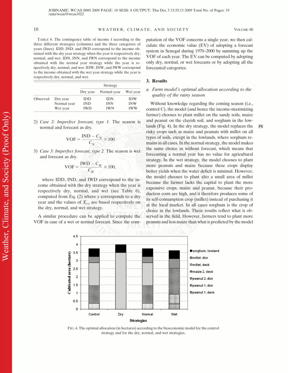
a. Farm model’s optimal allocation according to thequality of the rainy season

Without knowledge regarding the coming season (i.e.,

control C), the model (and hence the income-maximizing

farmer) chooses to plant millet on the sandy soils, maize

and peanut on the clayish soil, and sorghum in the low-

lands (F F4ig. 4). In the dry strategy, the model replaces the

risky crops such as maize and peanuts with millet on all

types of soils, except in the lowlands, where sorghum re-

mains in all cases. In the normal strategy, the model makes

the same choice as without forecast, which means that

forecasting a normal year has no value for agricultural

strategy. In the wet strategy, the model chooses to plant

more peanuts and maize because these crops display

better yields when the water deficit is minimal. However,

the model chooses to plant also a small area of millet

because the farmer lacks the capital to plant the more

expensive crops, maize and peanut, because their pro-

duction costs are high, and it therefore produces some of

its self-consumption crop (millet) instead of purchasing it

at the local market. In all cases sorghum is the crop of

choice in the lowlands. These results reflect what is ob-

served in the field. However, farmers tend to plant more

peanuts and less maize than what is predicted by the model

FIG. 4. The optimal allocation (in hectares) according to the bioeconomic model for the control

strategy and for the dry, normal, and wet strategies.

TABLE 6. The contingency table of income I according to the

three different strategies (columns) and the three categories of

years (lines). IDD, IND, and IWD correspond to the income ob-

tained with the dry year strategy when the year is respectively dry,

normal, and wet. IDN, INN, and IWN correspond to the income

obtained with the normal year strategy while the year is re-

spectively dry, normal, and wet. IDW, INW, and IWW correspond

to the income obtained with the wet year strategy while the year is

respectively dry, normal, and wet.

Strategy


Observed Dry year IDD IDN IDW

Normal year IND INN INW

Wet year IWD IWN IWW



Wea

ther

, Clim

ate,

and

Soc

iety

(Pro

of O

nly)

because peanut prices are guaranteed by the state whereas

prices for the other crops are not regulated. In the model,

the strategies are mainly driven by the yields and gross

margins of each crop (FF5 ig. 5). If the gross margins of

maize and peanuts are large when the rainy season is

wet, they are very small for a dry rainy season, even

smaller than the gross margins of millet or sorghum. The

risky character of maize and peanuts is also illustrated

by comparison of the standard deviation for each crop.

The standard deviation is computed from the values of

Table 4 with nine values per crop, corresponding to the

three considered types of soil and the three considered

types of rainy season. Maize and peanuts show large

standard deviations of yields compared to millet or sor-

ghum (Fig. 5).

To assess the importance of the effect of risk aversion

in driving the farmers’ strategies, we performed three

simulations of the model by varying the value of mi [see

Eq. (5)] to define high, low, and medium risk aversion

categories. When computing income per type of year

and per risk aversion (FF6 ig. 6), one can notice that income

for dry years increases with high risk aversion whereas

income for wet years decreases. It leads to a high vari-

ability of low risk aversion incomes whereas a high risk-

averse management tends to smooth income differences

from one type of year to another. The variability of in-

comes with a low sensitivity to risk is due to a variety of

management options chosen by the model that are close

to the ones described above (corresponding to the in-

termediate case of Fig. 6), with basically an competition

between cash crops for wet years and food crops for dry

years. On the other hand, the low variability of income

and the low mean income over the three types of years

for the high-risk aversion simulation comes from the

predominance of food crops (sorghum and millet) every

year to prevent risks of a bad year.

b. The economic value of using seasonal forecasts:Sensitivity analysis

To document the economic value of the use of sea-

sonal forecasts, we compare the income obtained with

no a priori information on the coming rainy season to

that obtained when the farmer adapts his strategy to

a priori information on the coming season. This value is

FIG. 5. (top) Gross margins (in Franc Communaute Financiere Africaine, FCFAAU12 ) of each

crop and each type of rainy season (dry, normal, and wet). (bottom) Standard deviation of

yields (kg ha21) for each crop. Peanut 1 and 2 correspond to the cultivation of peanut with two

levels of intensification (low and high). Maize 1, 2, and 3 correspond to the cultivation of maize

with three levels of intensification (low, medium, high).



Wea

ther

, Clim

ate,

and

Soc

iety

(Pro

of O

nly)

defined by the VOF (see section 2e) which is computed

separately for dry- and wet-year forecasts (TT7 able 7) in

order to assess which type of rainy season farmers may

find the most useful to know in advance. The VOFs for

dry and wet year forecasts show very different values.

The VOF of a dry year forecast is very high, up to 180%

in case of a perfect forecast. The losses resulting from an

imperfect forecast represent 9% or 28% of the income

obtained using the control strategy respectively in case

of a normal or a wet year. In contrast, the VOF of a wet

year forecast is low (17% respect to the control strat-

egy) and the cost of the error is high, with a loss of in-

come of 11% with the occurrence of a normal year and

70% with the occurrence of a dry year. It means that

predicting dryer rainy seasons is much more useful than

predicting the wetter ones. Indeed, on the one hand the

response to a wet year forecast introduces a high risk

with the increase of areas planted with cash crops such as

maize and peanuts that are highly vulnerable to drought.

On the other hand, the response to a dry year forecast

minimizes the climate risk by favoring robust crops such

as millet and sorghum.

Since forecasts are often probabilistic, we examine the

variations of the VOF of dry and wet years by varying

respectively the value of PD and PW from 1 (the de-

terministic case) to 0.33 (no forecast). FF7 igure 7 shows

that forecasts have an economic value when the proba-

bility of being in a particular tercile category reaches 0.4

for wet year forecasts and 0.5 for dry year forecasts. The

maximum economic value of dry (wet) year forecasts

is obtained with a probability greater than 0.6 (0.8) of

being in the lower (upper) tercile category, which is a

very strong probability shift when considering the out-

puts of the actual seasonal forecast products.

We now examine the sensitivity of the economic value

of the use of seasonal forecasts according to the accuracy

of the forecasts. To do so, we generate random forecasts

of the JAS Senegal rainfall index such as

X 5 Y 1 j 3 k,

where X is a random forecast, Y the JAS Senegal rainfall

index, and j a white-noise process that represents the

uncertainty of the forecast whose amplitude is defined by

a scale factor k. We then generate 10 000 random factors

by varying the value of k. A value of 0 for k indicates

a perfect forecast; the skill score decreases with the in-

crease of k. We then evaluate the performance of these

random forecasts X by computing the correlation with Y,

ROC scores, and the economic value (see sections 2d

and 2e). F F8igure 8 shows the EV of dry year forecasts

according to four measures of skill prediction of dry

years: the HR, the FAR, the HKS, and the correlation.

Several threshold values of the forecast skill can be de-

fined from Fig. 8. Forecast systems of dry years would

lead to benefits (e.g., only positive EV) with an HR, HKS,

and correlation with observations respectively greater

TABLE 7. The value of forecast (see section 2e) of the use of dry,

normal, and wet year forecasts. The VOF of the use of a dry year

forecast varies from 179.7% if the year is dry (perfect forecast) to

29.4% and 227.7% if the year is respectively normal or wet

(wrong forecast). The VOF of the use of a wet year forecast varies

from 16.5% if the year is wet (perfect forecast) to 210.8% and

270.1% if the year is respectively normal or dry (wrong forecast).

The prediction of a normal year shows a VOF of zero.

Predicted


Observed Dry year 179.7 0 270.1

Normal year 29.4 0 210.8

Wet year 227.7 0 16.5

FIG. 6. Net income (FCFA) for three levels of risk aversion and each type of rainy season

(dry, normal, and wet). The medium risk aversion level corresponds to the one chosen for the

Nioro du Rip typical farm.



Wea

ther

, Clim

ate,

and

Soc

iety

(Pro

of O

nly)

than 0.6, 0.7, and 0.6. In the same way, the FAR should be

lower than 0.2. These levels for skill scores are promis-

ing: a forecast system that is able to predict only 6 dry

years out of 10 would still be quite beneficial for farmers.

To expect only benefits from the adoption of the wet

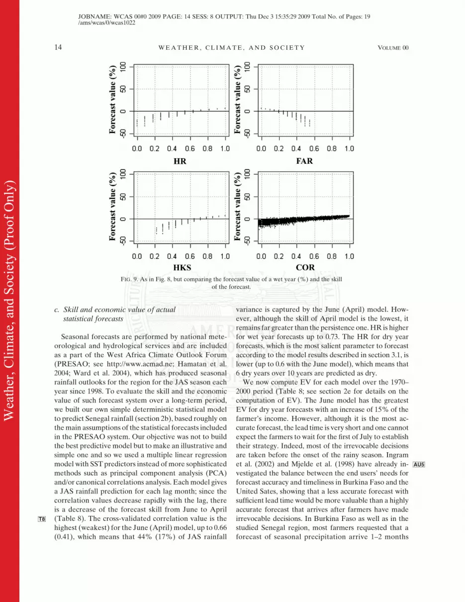
forecasts (F F9ig. 9), the forecast system needs to be more

skilful than the dry one, with an HR greater than 0.7,

an HKS greater than 0.75, and a correlation with ob-

servations greater than 0.8. The FAR should be lower

than 0.15.

FIG. 7. Value of the forecast (VOF) of dry years (black circles and full line) and wet years

(white circle and dashed line) with respect to the control strategy (%) according to the fore-

casted probability of being in the lower (for dry year forecasts) or upper (for wet year forecasts)

tercile category.

FIG. 8. Relationships between the forecast value of a dry year (%) and the skill of the

forecast. The skill of the forecast is assessed by the hit rate (HR), the false alarm rate (FAR),

the Hanssen and Kuipers score (HKS) and the correlation coefficient (COR). Results are based

on the generation of 10 000 virtual forecasts of the JAS Senegal rainfall index, where the un-

certainty of the forecast is modeled by adding noise to the rainfall time series.



Wea

ther

, Clim

ate,

and

Soc

iety

(Pro

of O

nly)

c. Skill and economic value of actualstatistical forecasts

Seasonal forecasts are performed by national mete-

orological and hydrological services and are included

as a part of the West Africa Climate Outlook Forum

(PRESAO; see http://www.acmad.ne; Hamatan et al.

2004; Ward et al. 2004), which has produced seasonal

rainfall outlooks for the region for the JAS season each

year since 1998. To evaluate the skill and the economic

value of such forecast system over a long-term period,

we built our own simple deterministic statistical model

to predict Senegal rainfall (section 2b), based roughly on

the main assumptions of the statistical forecasts included

in the PRESAO system. Our objective was not to build

the best predictive model but to make an illustrative and

simple one and so we used a multiple linear regression

model with SST predictors instead of more sophisticated

methods such as principal component analysis (PCA)

and/or canonical correlations analysis. Each model gives

a JAS rainfall prediction for each lag month; since the

correlation values decrease rapidly with the lag, there

is a decrease of the forecast skill from June to April

(TT8 able 8). The cross-validated correlation value is the

highest (weakest) for the June (April) model, up to 0.66

(0.41), which means that 44% (17%) of JAS rainfall

variance is captured by the June (April) model. How-

ever, although the skill of April model is the lowest, it

remains far greater than the persistence one. HR is higher

for wet year forecasts up to 0.73. The HR for dry year

forecasts, which is the most salient parameter to forecast

according to the model results described in section 3.1, is

lower (up to 0.6 with the June model), which means that

6 dry years over 10 years are predicted as dry.

We now compute EV for each model over the 1970–

2000 period (Table 8; see section 2e for details on the

computation of EV). The June model has the greatest

EV for dry year forecasts with an increase of 15% of the

farmer’s income. However, although it is the most ac-

curate forecast, the lead time is very short and one cannot

expect the farmers to wait for the first of July to establish

their strategy. Indeed, most of the irrevocable decisions

are taken before the onset of the rainy season. Ingram

et al. (2002) and Mjelde et al. (1998 AU5) have already in-

vestigated the balance between the end users’ needs for

forecast accuracy and timeliness in Burkina Faso and the

United Sates, showing that a less accurate forecast with

sufficient lead time would be more valuable than a highly

accurate forecast that arrives after farmers have made

irrevocable decisions. In Burkina Faso as well as in the

studied Senegal region, most farmers requested that a

forecast of seasonal precipitation arrive 1–2 months

FIG. 9. As in Fig. 8, but comparing the forecast value of a wet year (%) and the skill

of the forecast.



Wea

ther

, Clim

ate,

and

Soc

iety

(Pro

of O

nly)

before the expected onset of the rainy season—that is,

by late April or early May. This lead time would enable

them to optimize land allocation, to obtain seed of dif-

ferent varieties, and to prepare fields in different loca-

tions (Ingram et al. 2002). This lead time corresponds to

the April model in the present paper. Even if the cor-

relation between predicted and observed rainfall is

worst from the June model, the April model shows

a good ability to predict the dry years (HR 5 0.5) and it

thus presents a promising EV with an increase of about

14% of income with respect to the control strategy (i.e.,

with no a priori information). One can notice a non-

intuitive difference in EV for dry year forecasts between

the April model (EV 5 14%) and the May model, which

shows a weaker EV (EV 5 8.5%) although the lead time

is weaker, while the HR for dry year forecasts is the

same (HR 5 0.5). This difference results in the fact that

HR does not discriminate between the two types of error

in the case of an imperfect forecast (see section 2e), and

in the computation of VOF (and probably in reality) the

occurrence of a normal year or a wet year when the year

is forecast as a dry one does not have the same impact at

farm level.

d. Skill and economic value of DEMETERdynamical forecasts

We now evaluate the value of DEMETER dynamical

forecasts, which are based on seven coupled model sim-

ulations from a climate and an economic point of view

(TT9 able 9). The lag of these simulations is comparable to

the one of the April statistical model in the section above

and corresponds to the ideal timing for forecast as stated

by Senegal farmers. The skill scores are very low, with

most of the correlation coefficients with negative value

and ROC scores lower than the persistence ones. As

a matter of fact, EV is negative for all forecasts, which

means that no benefits can be expected by using them.

The inability of the DEMETER direct rainfall outputs to

reproduce the year-to-year variability of rainfall in the

western and central Sahel regions has already been docu-

mented by Bouali et al. (2008). Since variables relative to

the atmospheric dynamics are much more predictable and

reproducible than rainfall in a coupled GCM (Philippon

et al. 2008, manuscript submitted to Climate Dyn.), an

alternative approach is to combine in a statistical model

predictors computed from GCM outputs (Bouali et al.

2008; Mo and Thiaw 2002; Paeth and Hense 2003, Rogel

et al. 2006). Such statistical adaptations give very prom-

ising results, greatly increasing the forecast skill of July-

to-September rainfall in comparison with models’ direct

rainfall outputs (Garric et al. 2002; Bouali et al. 2008).

To restore the true potential of dynamic models, we will

therefore apply a correction to the rainfall DEMETER

outputs. This correction, much simpler than the one of

Bouali et al. (2008), is based on the assumption that the

large-scale variability is much more predictable than the

whole signal. The basic idea is that the first modes of

a PCA on JAS rainfall, which contain the large-scale

variability, are likely to be more predictable than a local

rainfall average (such as the JAS Senegal rainfall index

used in this study) and thus the partial reconstruction

of the JAS Senegal rainfall index with only these first

modes would improve its predictability. We apply PCA

separately on both observed and simulated JAS rainfall

over a large African domain (108S–308N, 208W–308E;

see F F10ig. 10).

The spatial structure of the first principal component

(PC) shows similarities in most of the simulations and in

the MMEM simulation, with a zonal maximum of co-

variance between 58 and 108N (Fig. 10). This structure is

shifted southward compared to the observations show-

ing a zonal maximum located between 108 and 158N.

This difference can be attributed to the southward bias

in the location of the ITCZ in most of the coupled

models (Bouali et al. 2008; Cook and Vizy 2006). The

correlations between the PC time series in the observa-

tions and in the models are generally significantly positive,

TABLE 8. The skill scores and economic value (EV) of statistical

forecasts based on the June, May, and April SST and based on

persistence. The skill of the forecast is assessed by the hit rate,

the false alarm rate, and the Hanssen and Kuipers score over the

1970–2000 period. Positive EVs are in bold.

Lag

Dry forecast Wet Forecast

COR HR FAR HKS EV HR FAR HKS EV

June 0.7 0.6 0.2 0.7 15.0 0.7 0.2 0.8 3.0

May 0.6 0.5 0.2 0.6 8.5 0.7 0.2 0.8 2.1

April 0.4 0.5 0.2 0.6 13.8 0.6 0.3 0.7 20.8

Pers 0.3 0.3 0.4 0.5 21.6 0.4 0.3 0.6 26.9

TABLE 9. The skill scores and economic value of DEMETER

dynamical forecasts. The skill of the forecast is assessed by the HR,

the FAR, and the HKS over the 1970–2000 period. The skill scores

and EV are given for each model and for the the multimodel en-

semble mean (MMEM).

Dry forecast Wet forecast


CNRM 20.3 0.2 0.4 0.4 211.2 0.3 0.4 0.4 216.5

CRFC 20.5 0.1 0.4 0.4 218.7 0.0 0.5 0.3 229.7

LODY 20.3 0.2 0.4 0.4 211.4 0.2 0.4 0.4 212.3

SCNR 20.4 0.1 0.4 0.3 221.1 0.2 0.4 0.4 214.7

SCWF 20.1 0.1 0.4 0.3 220.1 0.3 0.4 0.4 211.5

SMPI 0.0 0.4 0.3 0.6 20.9 0.3 0.4 0.4 211.5

UKMO 0.1 0.2 0.4 0.4 211.2 0.4 0.4 0.5 27.2

MMEM 20.2 0.2 0.4 0.4 216.0 0.2 0.5 0.4 216.9



Wea

ther

, Clim

ate,

and

Soc

iety

(Pro

of O

nly)

with a correlation coefficient of 0.33 for the MMEM

simulations, confirming our basic hypothesis of the better

predictability of the large-scale features. However, the

spatial structures of the second or the third PC (not

shown) show a large heterogeneity within models, re-

vealing internal variability of the models, and very few

positive and significant correlations are found with the

observed second and third PC. Therefore, only the first

PC will be used in the rest of this paper and we then

reconstruct the JAS Senegal observed and simulated

rainfall by using solely this PC.

The correlation between this reconstructed index and

the raw index in the observations is 0.79, which means

that 72% of the rainfall variance is explained by this first

mode of variability. The correlation between the simu-

lated reconstructed index (also called the corrected

simulations) and the observed Senegal rainfall has been

largely improved compared to the ones using raw model

rainfall outputs (T T10able 10) with three models—those of

the Centre National de Recherches Meteorologiques

(CNRM), SMPI, and the Met Office (UKMO)—with

a significant correlation coefficient value at 10% and the

FIG. 10. Spatial structure of the first PCA component on JAS rainfall in the observations (OBS), the multimodel ensemble mean

(MULTI), and the seven coupled models from DEMETER (Palmer et al. 2004).



Wea

ther

, Clim

ate,

and

Soc

iety

(Pro

of O

nly)

corrected MMEM giving the highest correlation up to

0.42. The same three models and the MMEM simulation

show an HKS greater than 0.5 while considering the

prediction of the dry years. Another interesting point is

that—once corrected with a simple PCA—the dynami-

cal forecasts perform as well as the statistical ones for

a comparable lag: the skill scores of the corrected MMEM

simulation are close to the one of the April model. Four

of the seven models showed positive economic value

for dry year forecasts (the maximum is reached by the

SMPI model with an EV 5 18.5%), but the expected

increase of income does not exceed 10% of the income

of the control strategy. The corrected MMEM simu-

lation shows a higher economic value (EV 5 19.6%)

for dry year forecasts than the individual model en-

semble means.

4. Conclusions

The methodology developed in this paper assesses the

value of seasonal forecasts for traditional farmers in

West Africa. It helps to fill the lack of quantitative

studies of seasonal climate forecasts in high-risk dryland

smallholder farming systems and in regions with rela-

tively good predictability of rainfall at a seasonal lead

time. It takes into account both climate and economic

valuations. The economic valuation relies on a simple

bioeconomic model calibrated on a typical farm in center

Senegal, which is used to simulate the farmers’ response

and resulting farm income to the dissemination and the

adoption of a forecast of rainfall categories. The appli-

cation of the model to forecasts of categories of total

seasonal rainfall (i.e., dryer than average, average, and

wetter than average) in a deterministic context (i.e.,

either 100% forecast accuracy or farmers’ decisions dic-

tated by the highest probability) has shown that predicting

dryer seasons is the most promising for these farmers.

In the case of an imperfect forecast, the adoption of a

wetter season forecast exposes the farmers to a high risk

of failure by favoring cash crops that are highly vulner-

able to drought. In addition, the response to a dryer

season forecast minimizes the climate risk by favoring

robust crops such as millet and sorghum. The economic

value of a dry forecast is thus very high, with an increase

of income of 80% with respect to the control strategy

in case of a perfect forecast. By investigating a large

number of hypothetic random forecasts, we were able to

estimate the forecast skill scores thresholds that need to

be achieved in order to generate benefits for farmers.

We have found than these skill scores were not as high as

we expected. For instance, a forecast system that is able

to predict 6 dry years over 10 years would be beneficial

for farmers. However, when considering probabilistic

forecasts, a very strong probability shift up to 0.6—

possibly more than available calibrated forecast models

for West Africa would ever produce—is required to shift

the conditional expected value of seasonal rainfall out-

side of the bounds of the middle tercile.

We applied our methodology to two state-of-the-art

approaches to climate predictions: statistical forecast

methods that are close to the ones included in the oper-

ational PRESAO system but are transposed in a deter-

ministic context and coupled atmosphere–ocean models

included in the DEMETER project. We found similar

skill and economic value of the statistical and dynamical

forecast methods by considering the same lead time

(April) and the same 31-yr hindcast period 1970–2000

and keeping only the large-scale variability of DEMETER

model outputs. Both forecast methods would have been

beneficial for Nioro du Rip farmers over this 31-yr period:

by using only the forecasts of dryer years they would have

increased their farm income by 13.8% for the statistical

model and 9.6% for the bias-corrected multimodel en-

semble mean. These two methods perform better than

the adoption of persistence forecasts, which is part of the

farmers’ common strategy.

The methodology and results presented in this paper

are very first steps in assessing the economic value of

seasonal forecasts in West Africa. It also brought for-

ward some clues about what needs to be done to im-

prove this evaluation:

d Our study does not take into account critical scale is-

sues raised by the use of the coarse spatial resolution

of climate models outputs. Because of high spatial

variability of rainfall, the weather experienced by the

farmers at the plot level in semiarid areas (Baron et al.

2005) might be quite different than the average value

in one 0.58 square grid. Downscaling climate predic-

tions (from the Senegal rainfall index grid cell to the

Nioro du Rip region in our case) would probably af-

fect the forecast skill and the economic value of the

forecasts.

TABLE 10. As in Table 9, but for the bias-corrected DEMETER

forecasts.

Dry forecast Wet forecast


CNRM 0.4 0.5 0.2 0.6 3.9 0.6 0.3 0.7 22.0

CRFC 0.1 0.6 0.2 0.7 3.9 0.4 0.3 0.6 23.7

LODY 20.2 0.3 0.3 0.5 213.8 0.2 0.4 0.4 215.2

SCNR 20.4 0.2 0.4 0.4 216.6 0.3 0.4 0.5 214.2

SCWF 20.6 0.2 0.4 0.4 218.0 0.1 0.5 0.3 228.2

SMPI 0.3 0.5 0.2 0.6 8.5 0.6 0.3 0.7 20.8

UKMO 0.4 0.6 0.2 0.7 4.8 0.6 0.2 0.7 0.7

MMEM 0.4 0.6 0.2 0.7 9.6 0.6 0.3 0.7 22.0



Wea

ther

, Clim

ate,

and

Soc

iety

(Pro

of O

nly)

d Another limitation of our study is that we focus on the

forecasts of categories of seasonal rainfall amount

(July to September), which is less critical to farmers

than predicting the onset and/or the end of the rainy

season and the distribution of rainfall within the sea-

son (Ingram et al. 2002). However, despite substantial

progress toward documenting the predictability of the

onset of the rainy seasons (Fontaine and Louvet 2006)

and the intraseasonal variability (Sultan et al. 2009),

there is up to now no routinely reliable forecast of such

variables in West Africa.d Since forecasts and insurance are complementary risk

management tools (Meza et al. 200AU6 9), their inter-

actions should be investigated. The utility of forecasts

can be increased when combined with insurance that

allow a risk-averse producer to make management

decisions based on probabilistic forecast information

that would have too much uncertainty to act on without

insurance (Carriquiry and Osgood 2007). Insurance

systems that can be driven by climate information have

already shown promising results in West Africa by re-

ducing the year-to-year variability of farmers’ income,

especially for cash crops such as maize and peanuts

(Berg et al. 2009).d Since the majority of farmers in the typical farm we

modeled are involved in cash crops, the model is bi-

ased toward cash crops—that is, enhancing the eco-

nomic value of forecasts. It would thus be important to

do the same kind of economic value assessment but for

subsistence farmers, which represent the majority of

farmers in the Sahel–Sudan. However, in these regions

they tend to produce only millet and have few alter-

native choices. Such study would thus require a much

more detailed representation of local practices (dif-

ferent varieties of millet, different sowing dates, use of

fertilizers, etc.) by using a crop model sensitive to

these options (D’Orgeval et al. 2009; Moeller et al.

2008) and to evaluate the most suitable ones based on

coupled simulations between crop models and sea-

sonal climate forecasts (Hansen et al. 2006).d Since seasonal climate forecasts are inherently prob-

abilistic, a better integration of the probabilistic in-

formation in the decision process is required to

improve the evaluation of forecasts (see, e.g., Mjelde

et al. 199AU7 6).

However, while it is true that such exhaustive model-

ing exercises allow quantitative estimates of the potential

benefits and risks of forecasts, they cannot fully capture

the complexity of real life decisions. Multidisciplinary

insights are required to analyze the dissemination, ac-

ceptance, and adoption of seasonal forecasts within local

knowledge frameworks (Magistro and Roncoli 2001;

Roncoli et al. 2000, 2002) in order to contribute in helping

African farmers to get the best from climate science in

a changing climatic environment.

Acknowledgments. This work has been funded by the

AMMA program. AMMA is managed by an international

scientific group and it is currently funded by a large

number of agencies, especially from France, the United

Kingdom, the United States, and Africa. It has been the

beneficiary of a major financial contribution from the

European Community’s Sixth Framework Research

Program. Detailed information on scientific coordination

and funding is available on the AMMA international web

site (see http://www.amma-international.org). This study

contributes also to the French ANR AUTREMENT

project (ANR-06-PADD-002). Thanks are also due to

IRD and CIRAD for additional financial support.

REFERENCES

Baron, C., B. Sultan, M. Balme, B. Sarr, S. Traore, T. Lebel,

S. Janicot, and M. Dingkuhn, 2005: From GCM grid cell to

agricultural plot: Scale issues affecting modelling of climate

impact. Philos. Trans. Roy. Soc., 360B, 2095–2108.

Berg, A., P. Quirion, and B. Sultan, 2009: Weather-index drought

insurance in Burkina Faso: Assessment of its potential interest

to farmers using historical data. Wea. Climate Soc., in press.

Bouali, L., N. Philippon, B. Fontaine, and J. Lemond, 2008: Per-

formance of DEMETER calibration for rainfall forecasting

purposes: Application to the July–August Sahelian rainfall.

J. Geophys. Res., 113, D15111, doi:10.1029/2007JD009403.

Cabrera, V. E., C. W. Fraisse, D. Letson, G. Podesta, and J. Novak,

2006: Impact of climate information on reducing farm risk

by optimizing crop insurance strategy. Trans. ASABE, 49,1223–1233.

Carriquiry, M., and D. Osgood, 2007: Index insurance, production

practices, and probabilistic climate forecasts. International

Research Institute for Climate and Society in the Earth In-

stitute at Columbia University Working Paper, 31 pp.

Cocks, K. D., 1968: Discrete stochastic programming. Manage. Sci.,

15, 72–79.

Cook, K. H., and E. K. Vizy, 2006: Coupled model simulations of

the West African Monsoon system: Twentieth- and twenty-

first-century simulations. J. Climate, 19, 3681–3703.

D’Orgeval, T., J. P. Boulanger, M. J. Capalbo, E. Guevara,

S. Meira, and O. Penalba, 2009: The value of seasonal climate

information for agricultural decision-making in the 3 CLARIS

sites. Climatic Change, in press AU8.

Folland, C. K., J. A. Owen, M. N. Ward, and A. W. Colman, 1991:

Prediction of seasonal rainfall in the Sahel region using em-

pirical and dynamical methods. J. Forecasting, 10, 21–56.

Fontaine, B., and S. Louvet, 2006: Sudan–Sahel rainfall onset:

Definition of an objective index, types of years, and experi-

mental hindcasts. J. Geophys. Res., 111, D20103, doi:10.1029/

2005JD007019.

——, N. Philippon, and P. Camberlin, 1999: An improvement of

June–September rainfall forecasting in the Sahel based upon

region April–May moist static energy content (1968–1997).

Geophys. Res. Lett., 26, 2041–2044.



Wea

ther

, Clim

ate,

and

Soc

iety

(Pro

of O

nly)

Garric, G., H. Douville, and M. Deque, 2002: Prospects for im-

proved seasonal predictions of monsoon precipitation over

Sahel. Int. J. Climatol., 22, 331–345.

Giannini, A., R. Saravanan, and P. Chang, 2003: Oceanic forcing of

Sahel rainfall on interannual to interdecadal time scales. Sci-

ence, 302, 1027–1030, doi:10.1126/science.1089357.

Hamatan, M., G. Mahe, E. Servat, J. E. Paturel, and A. Amani,

2004: Synthese et evaluation des previsions saisonnieres en

Afrique de l’Ouest. Secheresse, 15, 279–286.

Hammer, G. L., J. W. Hansen, J. G. Phillips, J. W. Mjelde, H. Hill,

A. Love, and A. Potgieter, 2001: Advances in application of

climate prediction in agriculture. Agric. Syst., 70, 515–553.

Hansen, J. W., 2002: Realizing the potential benefits of climate

prediction to agriculture: Issues, approaches, challenges. Agric.

Syst., 74, 309–330.

——, A. Challinor, A. Ines, T. Wheeler, and V. Moron, 2006:

Translating climate forecasts into agricultural terms: Ad-

vances and challenges. Climate Res., 33, 27–41.

Hazell, P. B. R., and R. D. Norton, 1986: Mathematical Pro-

gramming for Economic Analysis in Agriculture. MacMillan,

400 pp.

Ingram, K. T., M. C. Roncoli, and P. H. Kirshen, 2002: Opportu-

nities and constraints for farmers of West Africa to use sea-

sonal precipitation forecasts with Burkina Faso as a case study.

Agric. Syst., 74, 331–349.

Jacquet, F., and J. Pluvinage, 1997: Climatic uncertainty and farm

policy: A discrete stochastic programming model for cereal-

livestock farms in Algeria. Agric. Syst., 53, 387–407.

Janicot, S., S. Trzaska, and I. Poccard, 2001: Summer Sahel–ENSO

teleconnection and decadal time scale SST variations. Climate

Dyn., 18, 303–320.

Lobell, D. B., M. B. Burke, C. Tebaldi, M. D. Mastrandrea,

W. P. Falcon, and R. L. Naylor, 2008: Prioritizing climate

change adaptation needs for food security in 2030. Science,

319, 607–610.

Magistro, J., and M. C. Roncoli, 2001: Anthropological perspec-

tives and policy implications of climate change research. Cli-

mate Res., 19, 91–96.

Mason, S. J., and N. E. Graham, 1999: Conditional probabilities,

relative operating characteristics, and relative operating levels.

Wea. Forecasting, 14, 713–725.

Meza, F. J., J. W. Hansen, and D. Osgood, 2008: Economic value of

seasonal climate forecasts for agriculture: Review of ex-ante

assessments and recommendations for future research. J. Appl.

Meteor., 47, 1269–1286.

Michaelsen, J., 1987: Cross-validation in statistical climate forecast

models. J. Climate Appl. Meteor., 26, 1589–1600.

Mitchell, T. D., and P. D. Jones, 2005: An improved method of

constructing a database of monthly climate observations and

associated high-resolution grids. Int. J. Climatol., 25, 693–712.

Mjelde, J. W., S. T. Sonka, B. L. Dixon, and P. J. Lamb, 1988:

Valuing forecast characteristics in a dynamic agricultural

production system. Amer. J. Agric. Econ., 70, 674–684AU9 .

——, T. N. Thompson, C. N. Nixon, and P. J. Lamb, 1997: Utilising

a farm-level decision model to help prioritise future climate

prediction research needs. Meteor. Appl., 4, 161–170AU10 .

Mo, K. C., and W. M. Thiaw, 2002: Ensemble canonical correlation

prediction of precipitation over the Sahel. Geophys. Res. Lett.,

29, 1570, doi:10.1029/2002GL015075.

Moeller, C., I. Smith, S. Asseng, F. Ludwig, and N. Telcik, 2008:

The potential value of seasonal forecasts of rainfall categories—

Case studies from the wheatbelt in Western Australia’s Medi-

terranean region. Agric. For. Meteor., 148, 606–618.

Ogallo, L. A., M. S. Boulahya, and T. Keane, 2000: Applications of

seasonal to interannual climate prediction in agricultural

planning and operations. Agric. For. Meteor., 103, 159–166.

Oram, P. A., 1989: Sensitivity of agricultural production to climatic

change: An update. Proc. Int. Symp. on Climate Variability

and Food Security in Developing Countries, New Delhi, India,

IRRI, 25–44.

Paeth, H., and A. Hense, 2003: Seasonal forecasts of sub-Sahelian

rainfall using cross-validated model output statistics. Meteor.

Z., 12, 157–173.

Palmer, T. N., and Coauthors, 2004: Development of a European

multimodel ensemble system for seasonal-to-interannual pre-

diction (DEMETER). Bull. Amer. Meteor. Soc., 85, 853–872.

Philippon, N., F. Doblas Reyes, L. Bouali, and P. Ruti, 2008: Sea-

sonal reproducibility and predictability of the West African

monsoon in coupled GCMs. Climate Dyn., submitted AU11.

Rogel, P., Y. M. Tourre, V. Benoit, and L. Jarlan, 2006: Tropical

Atlantic moisture availability and precipitation over West

Africa: Application to DEMETER hindcasts. Geophys. Res.

Lett., 33, L21711, doi:10.1029/2006GL027178.

Roncoli, M. C., K. T. Ingram, and P. H. Kirshen, 2000: Can farmers

of Burkina Faso use rainfall forecasts? Pract. Anthropol., 22,24–28.

——, ——, and ——, 2002: Reading the rains: Local knowledge and

rainfall forecasting among farmers of Burkina Faso. Soc. Nat.

Resour., 15, 411–430.

Smith, T. M., R. W. Reynolds, T. C. Peterson, and J. Lawrimore,

2008: Improvements to NOAA’s historical merged land–

ocean surface temperature analysis (1880–2006). J. Climate,

21, 2283–2296.

Sultan, B., S. Janicot, and C. Correia, 2009: Medium lead-time

predictability of intraseasonal variability of rainfall in West

Africa. Wea. Forecasting, 24, 767–784.

Tauer, L., 1983: Target MOTAD. Amer. J. Agric. Econ., 65,

606–610.

Thornton, P. K., 2006: Ex ante impact assessment and seasonal

climate forecasts: Status and issues. Climate Res., 33, 55–65.

Ward, M. N., 1998: Diagnosis and short-lead time prediction of

summer rainfall in tropical North Africa at interannual and

multidecadal timescales. J. Climate, 11, 3167–3191.

——, and Coauthors, 2004: Seasonal-to-decadal predictability and

prediction of West African climate. CLIVAR Exchanges,

No. 9, International CLIVAR Project Office, Southampton,

United Kingdom, 14–20.

Wilks, D. S., 1997: Forecast value: Prescriptive decision studies.

Economic Value of Weather and Climate Forecasts, R. Katz

and A. Murphy, Eds., Cambridge University Press, 109–149.

——, R. Dmowska, D. Harmatan, and H. T. Rossby, 2006: Statis-

tical Methods in the Atmospheric Sciences. 2nd ed. Elsevier,

627 pp.

WMO, 2006: Standardized verification system (SVS) for long-

range forecasts (LRF). Attachment II-8, Manual on the

GDPFS (WMO No. 485), Vol. I, 17 pp. [Available online at

http://www.wmo.int/pages/prog/www/DPS/LRF/ATTACHII-

8SVSfrom%20WMO_485_Vol_I.pdf.]



Wea

ther

, Clim

ate,

and

Soc

iety

(Pro

of O

nly)

Documents

Estimating the Potential Economic Value of Seasonal Forecasts in West Africa: A Long-Term Ex-Ante Assessment in Senegal