Estimation of Alpine Grassland Forage Nitrogen ... - MDPI

remote sensing

Article

Estimation of Alpine Grassland Forage NitrogenCoupled with Hyperspectral Characteristics duringDifferent Growth Periods on the Tibetan Plateau

Jinlong Gao 1,2 , Tiangang Liang 1,*, Jianpeng Yin 1, Jing Ge 1, Qisheng Feng 1, Caixia Wu 1,Mengjing Hou 1, Jie Liu 1 and Hongjie Xie 2

1 State Key Laboratory of Grassland Agro-Ecosystems, Key Laboratory of Grassland Livestock IndustryInnovation, Ministry of Agriculture and Rural Affairs, Engineering Research Center of Grassland Industry,Ministry of Education, College of Pastoral Agriculture Science and Technology, Lanzhou University,Lanzhou 730000, China

2 Center for Advanced Measurements in Extreme Environments and Department of Geological Sciences,University of Texas at San Antonio, San Antonio, TX 78249, USA

* Correspondence: [email protected]; Tel.: +86-931-981-5306; Fax: +86-931-891-0979

Received: 2 August 2019; Accepted: 4 September 2019; Published: 6 September 2019��

Abstract: The applicability of hyperspectral remote sensing models for forage nitrogen (N) retrievalduring different growth periods is limited. This study aims to develop a multivariate model feasiblefor estimating the forage N for the growth periods (June to November) in an alpine grasslandecosystem. The random forest (RF) algorithm is employed to determine the optimum combinationsof 38 spectral variables capable of capturing dynamic variations in forage N. The results show that (1)throughout the growth period, the red-edge first shifts toward longer wavelengths and then shiftstoward shorter wavelengths, the amplitude (AMP) and absorption depth (AD) gradually decrease,and the absorption position (AP) changes slightly; (2) the importance of spectral variables for forageN estimation differs during the different growth periods; (3) the multivariate model achieves betterresults for the first four periods (June to October) than for the last period (when the grass is completelysenesced) (V-R2: 0.58–0.68 versus 0.23); and (4) for the whole growth period (June to November),the prediction accuracy of the general N estimation model validated by the unknown growth period islower than that validated by the unknown location (V-R2 is 0.28 and 0.55 for the validation strategiesof Leave-Time-Out and Leave-Location-Out, respectively). This study demonstrates that the changesin the spectral features of the red wavelength (red-edge position, AMP and AD) are well coupledwith the forage N content. Moreover, the development of a multivariate RF model for estimatingalpine grasslands N content during different growth periods is promising for the improvement ofboth the stability and accuracy of the model.

Keywords: alpine grassland; hyperspectral characteristics; nitrogen; growth periods; Tibetan Plateau

1. Introduction

Nitrogen (N) is a key nutrient for vegetation growth and reproduction and plays an important rolein the sustainability of natural grassland resources and animal husbandry on the Tibetan Plateau [1,2].As a crucial component of proteins, nucleic acids, phospholipids, and chlorophyll in plants, N affectsplant photosynthesis and water absorption [3–5]. Insufficient N supply could result in changes in theexternal morphology and internal metabolism of plants. According to these changes, correspondingagricultural practices should be implemented to ensure the N status of the plants [6]. The accurateand efficient monitoring of the spatial distribution characteristics and seasonal dynamics of forage N

Remote Sens. 2019, 11, 2085; doi:10.3390/rs11182085 www.mdpi.com/journal/remotesensing

http://www.mdpi.com/journal/remotesensing

http://www.mdpi.com

https://orcid.org/0000-0003-1188-8271

https://orcid.org/0000-0003-3516-1210

http://www.mdpi.com/2072-4292/11/18/2085?type=check_update&version=1

http://dx.doi.org/10.3390/rs11182085

http://www.mdpi.com/journal/remotesensing

Remote Sens. 2019, 11, 2085 2 of 19

contribute to the improvement of livestock productivity and the maintenance of the safety and healthof alpine grassland ecosystems.

Hyperspectral remote sensing of grassland has been widely used in recent studies, including themonitoring of the nutritional status, aboveground biomass (AGB) and coverage of grasslands [7–10],species recognition [11,12], and health assessments [13]. In particular, the development of estimationmodels and the spatial mapping of forage N, based on a wide variety of hyperspectral spectrometersand sensors, has been a popular research topic [8,14,15]. Studies have indicated that several specificknown absorption bands for N, proteins, and chlorophyll (i.e., 640 nm, 910 nm, 1510 nm, and 2300 nm)can be successfully used for forage N estimation [14,16–19]. Moreover, some often-used red-edgeparameters, such as the red-edge slope, red-edge vegetation indexes (VIs), and red-edge position (REP),have a strong relationship with forage N [20,21]. Hence, some scholars have successfully estimatedand mapped forage N at the regional level using new-generation, high-resolution multispectralsensors (i.e., Sentinel-2, RapidEye, and WorldView-2) equipped with specialized red-edge wavebandssuitable for detecting vegetation growth information [15,21]. Most studies have employed empiricalspectral VIs to map forage N, such as the soil-adjusted vegetation index (SAVI), normalized differencevegetation index (NDVI), normalized difference nitrogen index (NDNI), and structure-independentpigment index (SIPI) [9,14,22]. The aforementioned spectral variables, VIs, and absorption featuresthat are all sensitive to N, have a significant effect on monitoring the spatial variation and distributioncharacteristics of forage N. However, although the aforementioned studies yielded high N estimationaccuracy, the generality and applicability of the spectral indexes were rarely discussed.

As a result of the differences in the vegetation spectral reflectance and canopy structure ofgrasslands in different ecological regions, nutritional stresses, and growth periods, the accuracy ofhyperspectral remote sensing models generally has certain limitations [23,24]. The growth period offorage has a strong correlation with the changes and distribution of N content, and it significantly affectsthe characteristics and morphology of the vegetation canopy spectrum. Most of the aforementionedhyperspectral parameters (i.e., VIs and absorption features) were proposed based on a specificgrowth period, especially the vigorous growing stage when the effect of biomass on N can beminimized [8,9]. Moreover, most studies have focused on the detection of spatial differences in forageN during a particular period without considering changes in the temporal dimension (different growthperiods) [25,26]. Although these spectral variables have shown great potential in estimating N, whethertheir ability to estimate N differs during different growth periods should be investigated. In conclusion,many factors contribute to the different sensitivities of spectral variables to the physiological parametersof vegetation. Therefore, it is significant to determine spectral variables suitable for estimating theforage N by developing a stable, universal, and high-precision inversion model.

Many nonparametric machine learning algorithms, for example, artificial neural network (ANN),support vector machine (SVM), and random forest (RF), have been employed for variable selection andmodel development because of their superior performance in addressing nonlinear and multivariateproblems in comparison with traditional algorithms. With particular respect to regression algorithms,RF was found to be outstanding when compared with other methods because it has a superiorcapability to correct incorrect and missing data [27] and circumvents overfitting and multicollinearityproblems [28]. In addition, RF can also rank the importance of variables that contributes to a model,suggesting that variable selection can be achieved with this distinct advantage. Recent studies haveindicated that the use of RF for the estimation of forage biochemical parameters (e.g., N, phosphorus,lignin, cellulose) is very promising, both in an African tropical grassland and an alpine grasslandecosystem [15,29,30].

Therefore, to further explore the applicability of spectral variables during different growthperiods, this paper presents a study based on five field experiments across the growth periods onalpine grassland in the Tibetan Plateau (from the end of June to the middle of November) and theRF algorithms to (1) analyze the variations in forage N and the canopy spectrum; (2) explore therelationship between spectral variables and forage N; (3) identify the VIs and spectral features that

Remote Sens. 2019, 11, 2085 3 of 19

are sensitive to forage N based on RF algorithm; and (4) establish multivariate models to estimateforage N during different growth periods. According to this study, we expect to improve the predictionaccuracy of the hyperspectral forage N inversion model and provide technical support for the accuratemonitoring of vegetation growth.

2. Materials and Methods

2.1. Study Area

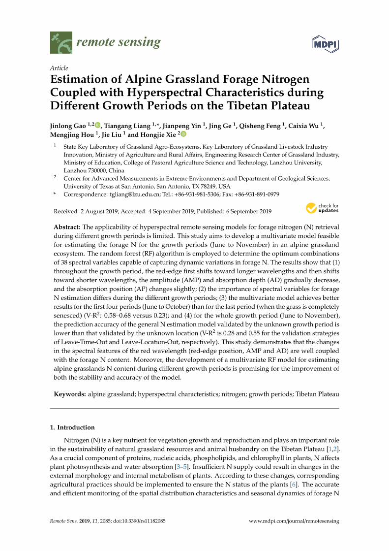
The study area (33.11◦N–35.57◦N, 100.77◦E–102.98◦E) lies in the northeastern margin of theTibetan Plateau, and it has an average altitude of over 3000 m. As shown in Figure 1, the area includesthree counties, from the northeast to southwest: Xiahe, Luqu, and Maqu. The area is characterizedby a continental plateau climate with an average annual temperature of 1.6–13.6 ◦C, with an averageannual precipitation of 400–800 mm, and it exhibits significant spatial differences and temporalvariations. The study area is rich in natural alpine grassland resources and 87% of its land is coveredwith grassland (18,978.3 km2); the major grassland types are alpine meadow and alpine steppe. Thedominant species mainly include Stipa aliena, Festuca ovina, Poa pratensis var. pratensis, Kobresia capillifolia,and Potentilla chinensis. Fertilization and mowing are rarely carried out in the study area, and grasslandutilization is mainly dominated by four-season rotational grazing and grazing blocked by fencing.

Remote Sens. 2019, 11, x FOR PEER REVIEW 3 of 19

are sensitive to forage N based on RF algorithm; and (4) establish multivariate models to estimate forage N during different growth periods. According to this study, we expect to improve the prediction accuracy of the hyperspectral forage N inversion model and provide technical support for the accurate monitoring of vegetation growth.

2. Materials and Methods

2.1. Study Area

The study area (33.11°N–35.57°N, 100.77°E–102.98°E) lies in the northeastern margin of the Tibetan Plateau, and it has an average altitude of over 3000 m. As shown in Figure 1, the area includes three counties, from the northeast to southwest: Xiahe, Luqu, and Maqu. The area is characterized by a continental plateau climate with an average annual temperature of 1.6–13.6 °C, with an average annual precipitation of 400–800 mm, and it exhibits significant spatial differences and temporal variations. The study area is rich in natural alpine grassland resources and 87% of its land is covered with grassland (18,978.3 km2); the major grassland types are alpine meadow and alpine steppe. The dominant species mainly include Stipa aliena, Festuca ovina, Poa pratensis var. pratensis, Kobresia capillifolia, and Potentilla chinensis. Fertilization and mowing are rarely carried out in the study area, and grassland utilization is mainly dominated by four-season rotational grazing and grazing blocked by fencing.

Figure 1. Study area at the northeastern margin of the Tibetan Plateau, with the four sampling areas (GJ, YLJ, XC, and AZ) from north to south.

2.2. Grassland Observation Data

Four sampling areas (GJ, YLJ, XC, and AZ) were set in the study area from north to south according to the spatial representation, accessibility and management mode, as shown in Figure 1. Among those sampling areas, AZ is located in the Azi yak propagation bases of Maqu County, XC is located in the Xicang Township of Luqu County, and YLJ and GJ are located in the Yaliji Township and Ganjia Township of Xiahe County, respectively. In comparison with other sampling areas, XC is nearest to YLJ, and the distance between them is approximately 30 km. In each area, five sample plots

Figure 1. Study area at the northeastern margin of the Tibetan Plateau, with the four sampling areas(GJ, YLJ, XC, and AZ) from north to south.

2.2. Grassland Observation Data

Four sampling areas (GJ, YLJ, XC, and AZ) were set in the study area from north to south accordingto the spatial representation, accessibility and management mode, as shown in Figure 1. Among thosesampling areas, AZ is located in the Azi yak propagation bases of Maqu County, XC is located inthe Xicang Township of Luqu County, and YLJ and GJ are located in the Yaliji Township and GanjiaTownship of Xiahe County, respectively. In comparison with other sampling areas, XC is nearest to YLJ,

Remote Sens. 2019, 11, 2085 4 of 19

and the distance between them is approximately 30 km. In each area, five sample plots were selectedas permanent observation sites. The distance between the plots is limited to approximately 3 km inconsideration of the homogeneity of the plot, and the dimension of each plot is 100 m × 100 m. Fivesubplots (0.5 m × 0.5 m) were set up within each plot to obtain the plot variability.

During the grassland growth period (GP, June to November), five field investigations beganon 24 June, 27 July, 30 August, 27 September, and 15 November 2017. Each fieldwork campaignlasted approximately four to six days; to present the specific time of each field work more intuitively,the beginning date of every investigation was used as a reference for naming the period, namely,GP170624, GP170727, GP170830, GP170927, and GP171115. GP-ALL is used to represent the wholegrowth period from June to November. A total of 100 sample were collected. In each subplot,the canopy reflectance spectra of the mixed grassland community were measured 10 times using aportable ASD Field Spec Pro FR2500 spectroradiometer (Analytical Spectral Devices Inc., Boulder,CO, USA) with spectral range of 350–2500 nm and a view angle of 25◦ between 10:00 and 14:00 on asunny day. The height of the sensor was approximately 1 m from the plant canopy. The reflectancespectra were then averaged as the final spectrum of each plot for the data. In addition, we collected theconventional observations for each subplot, including the geographic location, grassland communityheight and coverage, dominant species, dead component percent of grassland and AGB; grass sampleswere also collected.

After each investigation, all the grass samples were transferred to the lab for further physicalprocessing (oven-dried at 65 ◦C for 48 h, smashed and sieved) and chemical analysis. After the sampleswere boiled and digested with concentrated H2SO4 solution, dehydrated and carbonized, and a seriesof oxidation reactions were performed. A FIAstar 5000 flow injection analyzer was used to quantifythe N content. The method uses K2SO4/CuSO4 as a catalyst, and the operation steps are simple andfast and do not interfere with the quantification of N elements.

2.3. Spectral Variables

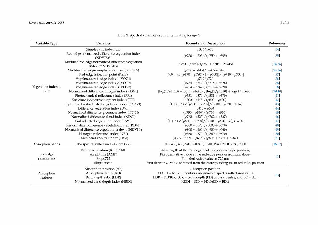
Table 1 summarizes the 38 spectral variables, including 20 VIs, 10 absorption bands, 4 red-edgeparameters, and 4 absorption features, which are widely used for estimating forage N. This study aimsto assess the performance of all these variables in the estimation of N during different growth periodsof grassland.

Narrow-band VIs has been widely used to qualitatively and quantitatively evaluate the growthstatus of grasslands. The specific known protein, chlorophyll, and N absorption bands have beensuccessfully used for the estimation of grass N [14,16,19]. The red-edge parameters, such as REP,amplitude (AMP), Slope725 and Slope_mean, have shown to be significantly correlated with the Nof vegetation [31]. The red-edge parameters were calculated based on the first derivative spectrumto effectively reduce the interference of soil and the atmospheric background [32]. Studies have alsofound that the absorption features of the absorption position (AP), absorption depth (AD), normalizedband depth index (NDBI) and band depth ratio (BDR) in the red-edge range (550–750 nm) based oncontinuum-removed spectra reflectance can effectively extract the biochemical parameters of grasslandvegetation, especially N and chlorophyll [8,9,33].

Remote Sens. 2019, 11, 2085 5 of 19

Table 1. Spectral variables used for estimating forage N.

Variable Type Variables Formula and Description References

Vegetation indexes(VIs)

Simple ratio index (SR) ρ800/ρ670 [34]Red-edge normalized difference vegetation index

(NDVI705) (ρ750− ρ705)/(ρ750 + ρ705) [35]

Modified red-edge normalized difference vegetationindex (mNDVI705)

(ρ750− ρ705)/(ρ750 + ρ705− 2ρ445) [24,36]

Modified red-edge simple ratio index (mSR705) (ρ750− ρ445)/(ρ705− ρ445) [24,36]Red-edge inflection point (REIP)

{700 + 40[(ρ670 + ρ780)/2− ρ700]

}/[(ρ740− ρ700)] [37]

Vogelmann red-edge index 1 (VOG1) ρ740/ρ720 [38]Vogelmann red-edge index 2 (VOG2) (ρ734− ρ747)/(ρ715 + ρ726) [38]Vogelmann red-edge index 3 (VOG3) (ρ734− ρ747)/(ρ715 + ρ720) [38]

Normalized difference nitrogen index (NDNI) [log(1/ρ1510) − log(1/ρ1680)]/[log(1/ρ1510) + log(1/ρ1680)] [39,40]Photochemical reflectance index (PRI) (ρ531− ρ570)/(ρ531 + ρ570) [41]

Structure insensitive pigment index (SIPI) (ρ800− ρ445)/(ρ800− ρ680). [42]Optimized soil-adjusted vegetation index (OSAVI) [(1 + 0.16) × (ρ800− ρ670)]/(ρ800 + ρ670 + 0.16) [43]

Difference vegetation index (DVI) ρ810− ρ680 [44]Normalized difference greenness index (NDGI) (ρ750− ρ550)/(ρ750 + ρ550). [45]

Normalized difference cloud index (NDCI) (ρ762− ρ527)/(ρ762 + ρ527) [46]Soil-adjusted vegetation index (SAVI) [(1 + L) × (ρ800− ρ670)]/(ρ800 + ρ670 + L), L = 0.5 [47]

Renormalized difference vegetation index (RDVI) (ρ800− ρ670)/(ρ800 + ρ670) [48]Normalized difference vegetation index 1 (NDVI 1) (ρ900− ρ660)/(ρ900 + ρ660) [49]

Nitrogen reflectance index (NRI) (ρ560− ρ670)/(ρ560 + ρ670) [50]Three-band spectral index (TBSI) (ρ605− ρ521− ρ682)/(ρ605 + ρ521 + ρ682) [51]

Absorption bands The spectral reflectance at λ nm (Rλ) Λ = 430, 460, 640, 660, 910, 1510, 1940, 2060, 2180, 2300 [16,52]

Red-edgeparameters

Red-edge position (REP) AMP Wavelength of the red-edge peak (maximum slope position)

[31]Amplitude (AMP) First derivative value at the red-edge peak (maximum slope)Slope725 First derivative value at 725 nm

Slope_mean First derivative value obtained from the corresponding mean red-edge position

Absorptionfeatures

Absorption position (AP) Absorption position

[53]Absorption depth (AD) AD = 1 − R′, R′ = continuum-removed spectra reflectance valueBand depth ratio (BDR) BDR = BD/BDc, BDc = band depth (BD) of band centre, and BD = AD

Normalized band depth index (NBDI) NBDI = (BD − BDc)/(BD + BDc)

Remote Sens. 2019, 11, 2085 6 of 19

2.4. Data Analysis and Modeling

2.4.1. RF Algorithm

The nonparametric and multivariate RF algorithm is used to establish a forage N estimation modelfrom different spectral variables during different growth periods. RF can improve the performanceof classification and regression trees (CARTs) through the use of a multitude of decision trees.The algorithm was developed by and is commonly used to solve complicated multiple regressionproblems [27]. The advantages of this algorithm include being less prone to overfitting, handlinghighly nonlinear data, exhibiting strong anti-noise ability, showing high accuracy, and having relativelysimple implementation [54,55]. When using the RF algorithm, it is necessary to optimize three pivotalparameters, mtry (number of predictors tested at each node), ntree (number of regression trees),and nodesize (minimal size of the terminal nodes of the trees). In this study, the RF program isprocessed using MATLAB 2016a software.

2.4.2. Variable Selection

For different growth periods, the sequential backward search (SBS) method, based on the RFalgorithm, is used to determine feature variables. SBS relies on the importance of each spectral variable,which is calculated by measuring the percent increase of the root mean squared error (RMSE) whenthe out-of-bag (OOB) data of each variable are permuted while all others remain unchanged. We rankthe variables (importance not equal to 0) by importance (from large to small) and then evaluate theprediction ability of each RF model, which was established by the first n variables. Finally, we choosethe feature set with the least number of variables and the optimal prediction ability as a result of featureselection. For the whole growth period, the forward feature selection (FFS) algorithm that works inconjunction with target-oriented validation is used to determine variables to improve the generalizationability of the model. The algorithm first tunes and trains the RF models using all possible combinationsof any two spectral variables. The best initial model in view to target oriented performance is kept.Then, the number of variables is iteratively increased. The improvement of the model is tested for eachadditional predictor using target-oriented cross-validation (CV). The process stops when none of theremaining variables decreases the error of the current best model. Finally, the predictor variables withbest modeling performance is determined as the feature variables. The details of this algorithm can befound in Meyer et al. [56].

2.4.3. Validation Strategies

When establishing the RF model of forage N during different growth periods using thecorresponding feature variables, we iterate the two core parameters (ntree and mtry) and choose thedefault values for the other parameters (e.g., nodesize, minimum impurity split, minimum samplesleaves, and minimum samples splits). The ntree values increase from 10 to 1000 in intervals of 10 foreach iteration, with a total of 100 iterations, and mtry is increased from 1 to m (m is the number ofvariables) in intervals of 1 each time for a total of m iterations.

To assess the performance and stability of all models (i.e., models of different growth periodsand whole growth period) in forage N estimation, Leave-One-Out (LOO) CV is used in this studybecause of its merits of unbiased estimation and outlier detection [57]. Moreover, to evaluate theprediction performance of the general model on unknown locations (sample area) and unknownpoints in time (growth period), three “target-oriented” validation strategies are used is this study:Leave-Time-Out (LTO) CV, Leave-Location-Out (LLO) CV and Leave-Location-and-Time-Out (LLTO)CV [56]. The goodness of fit of the measured and simulated forage N is evaluated by the coefficientof determination (R2), mean absolute error (MAE), RMSE, and coefficient of variation in the RMSE(CVRMSE) (Equation (1)).

Remote Sens. 2019, 11, 2085 7 of 19

CVRMSE (%) =

√∑ni=1(yi − yi)

2

n×

100y

(1)

where yi and yi are the N values of the test set for the simulated and measured; y is the measuredmean value; and n equals the sample size of the test dataset. If the CVRMSE < 10%, the predictivecapability is considered excellent; if the CVRMSE ranges from 10–20%, the predictive power is good;if the CVRMSE > 20%, the predictive performance is unsatisfactory.

3. Results

3.1. Variations in Forage N Contents and Reflectance Spectra during Different Growth Periods

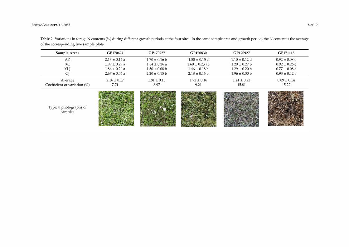
The highest N content was observed at site GJ and the lowest at site YLJ during the differentgrowth periods, as shown in Table 2. The overall forage N contents of different sampling areas duringdifferent growth periods show a clear decreasing trend with plant growth (P < 0.05). The forageN content in AZ is significantly different in the different growth periods (P < 0.05), indicating thatthere is significant spatial heterogeneity of grassland vegetation in this sampling area. Moreover,significant differences are not observed in the N contents in YLJ and GJ among GP170727, GP170830,and GP170927. In addition, the mean forage N content of the four sampling areas ranges from 0.89% to2.16% throughout the growth period and presents a coefficient of variation of 7.71–15.81%. In particular,the coefficient of variation of GP170927 and GP171115 (15.81% and 15.22%) are much greater thanthose of the other periods, indicating that a large spatial difference occurs in the forage N content inthe last two periods. From the typical photographs of samples during different growth periods, someinformation about the status of the grass can be obtained (i.e., color, morphology, and blossom).

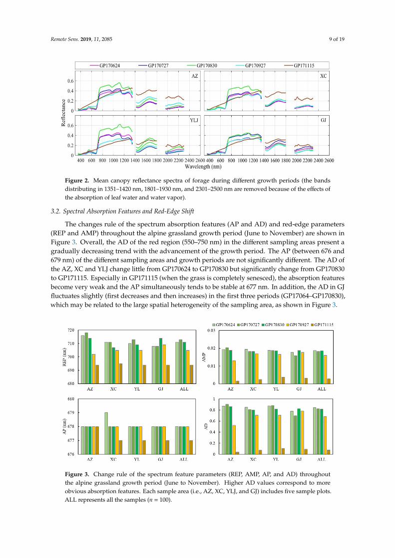
The changes in canopy spectral reflectance at the four sampling areas during different growthperiods, as shown in Figure 2. Overall, from the early period of forage growth (GP170624) to thevigorous growth period (GP170830), the plant mainly undergoes vegetative and reproductive growth.The vegetative stage refers to the developmental period comprising leaf growth and development,and the grass grows rapidly and the vegetation coverage increases gradually. The absorption of thevisible region by the grass canopy is obviously enhanced, and the reflectance in the visible regiondecreases gradually. In addition, the absorption in the red valley between 650 and 710 nm becomesmore obvious, and the reflectance in the near-infrared bands also increases significantly due to multiplescattering. After the vigorous grass growth period, the vegetation coverage decreases gradually andthe forage stops growing and begins to senesce. As the grass gradually senesces, the absorptionof the visible region by the grass gradually weakens, the reflectance in the visible region increaseswhile the near-infrared region decreases significantly (GP170830 to GP170927). When the grass iscompletely senesced in November (GP171115), the spectrum is similar to the spectral characteristics ofthe soil, showing a slowly increasing trend within the wavelengths from 350–1350 nm without obviousabsorption or reflection features. In addition, the higher shortwave near-infrared (1420–1800 nmand 1930–2300 nm) reflectance might be largely due to less water absorption in senesced grass.The absorption features on the spectral curve (i.e., obvious absorption valleys and reflection peaks)are gradually weakened with the advancement of the growth period, which may be related to thebiochemical parameters of the forage.

Remote Sens. 2019, 11, 2085 8 of 19

Table 2. Variations in forage N contents (%) during different growth periods at the four sites. In the same sample area and growth period, the N content is the averageof the corresponding five sample plots.

Sample Areas GP170624 GP170727 GP170830 GP170927 GP171115

AZ 2.13 ± 0.14 a 1.70 ± 0.16 b 1.58 ± 0.15 c 1.10 ± 0.12 d 0.92 ± 0.08 eXC 1.99 ± 0.29 a 1.84 ± 0.26 a 1.60 ± 0.23 ab 1.29 ± 0.27 b 0.92 ± 0.26 cYLJ 1.86 ± 0.20 a 1.50 ± 0.08 b 1.46 ± 0.18 b 1.29 ± 0.20 b 0.77 ± 0.08 cGJ 2.67 ± 0.04 a 2.20 ± 0.15 b 2.18 ± 0.16 b 1.96 ± 0.30 b 0.93 ± 0.12 c

Average 2.16 ± 0.17 1.81 ± 0.16 1.72 ± 0.16 1.41 ± 0.22 0.89 ± 0.14Coefficient of variation (%) 7.71 8.97 9.21 15.81 15.22

Typical photographs ofsamples


Table 2. Variations in forage N contents (%) during different growth periods at the four sites. In the same sample area and growth period, the N content is the average of the corresponding five sample plots.

Sample Areas GP170624 GP170727 GP170830 GP170927 GP171115 AZ 2.13 ± 0.14 a 1.70 ± 0.16 b 1.58 ± 0.15 c 1.10 ± 0.12 d 0.92 ± 0.08 e XC 1.99 ± 0.29 a 1.84 ± 0.26 a 1.60 ± 0.23 ab 1.29 ± 0.27 b 0.92 ± 0.26 c YLJ 1.86 ± 0.20 a 1.50 ± 0.08 b 1.46 ± 0.18 b 1.29 ± 0.20 b 0.77 ± 0.08 c GJ 2.67 ± 0.04 a 2.20 ± 0.15 b 2.18 ± 0.16 b 1.96 ± 0.30 b 0.93 ± 0.12 c

Average 2.16 ± 0.17 1.81 ± 0.16 1.72 ± 0.16 1.41 ± 0.22 0.89 ± 0.14 Coefficient of variation (%) 7.71 8.97 9.21 15.81 15.22

Typical photographs of samples





















Remote Sens. 2019, 11, 2085 9 of 19Remote Sens. 2019, 11, x FOR PEER REVIEW 9 of 19

Figure 2. Mean canopy reflectance spectra of forage during different growth periods (the bands distributing in 1351–1420 nm, 1801–1930 nm, and 2301–2500 nm are removed because of the effects of the absorption of leaf water and water vapor).

3.2. Spectral Absorption Features and Red-Edge Shift

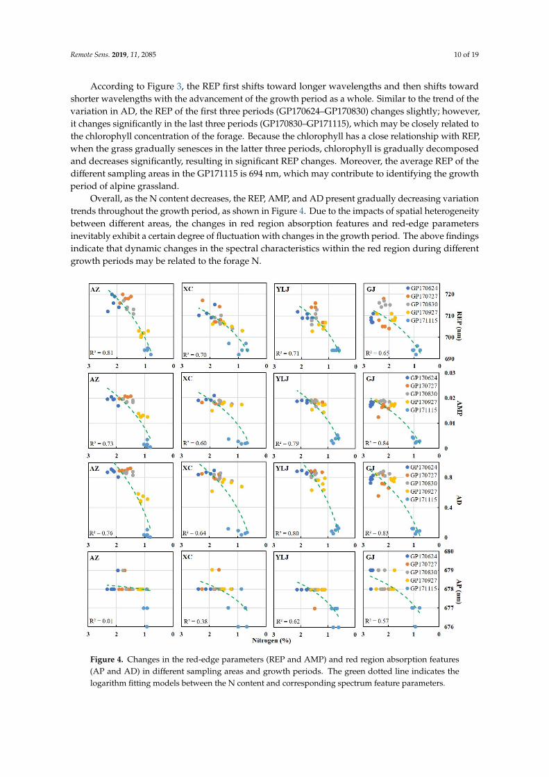
The changes rule of the spectrum absorption features (AP and AD) and red-edge parameters (REP and AMP) throughout the alpine grassland growth period (June to November) are shown in Figure 3. Overall, the AD of the red region (550–750 nm) in the different sampling areas present a gradually decreasing trend with the advancement of the growth period. The AP (between 676 and 679 nm) of the different sampling areas and growth periods are not significantly different. The AD of the AZ, XC and YLJ change little from GP170624 to GP170830 but significantly change from GP170830 to GP171115. Especially in GP171115 (when the grass is completely senesced), the absorption features become very weak and the AP simultaneously tends to be stable at 677 nm. In addition, the AD in GJ fluctuates slightly (first decreases and then increases) in the first three periods (GP17064–GP170830), which may be related to the large spatial heterogeneity of the sampling area, as shown in Figure 3.

Figure 3. Change rule of the spectrum feature parameters (REP, AMP, AP, and AD) throughout the alpine grassland growth period (June to November). Higher AD values correspond to more obvious absorption features. Each sample area (i.e., AZ, XC, YLJ, and GJ) includes five sample plots. ALL represents all the samples (n = 100).

According to Figure 3, the REP first shifts toward longer wavelengths and then shifts toward shorter wavelengths with the advancement of the growth period as a whole. Similar to the trend of

Figure 2. Mean canopy reflectance spectra of forage during different growth periods (the bandsdistributing in 1351–1420 nm, 1801–1930 nm, and 2301–2500 nm are removed because of the effects ofthe absorption of leaf water and water vapor).


The changes rule of the spectrum absorption features (AP and AD) and red-edge parameters(REP and AMP) throughout the alpine grassland growth period (June to November) are shown inFigure 3. Overall, the AD of the red region (550–750 nm) in the different sampling areas present agradually decreasing trend with the advancement of the growth period. The AP (between 676 and679 nm) of the different sampling areas and growth periods are not significantly different. The AD ofthe AZ, XC and YLJ change little from GP170624 to GP170830 but significantly change from GP170830to GP171115. Especially in GP171115 (when the grass is completely senesced), the absorption featuresbecome very weak and the AP simultaneously tends to be stable at 677 nm. In addition, the AD in GJfluctuates slightly (first decreases and then increases) in the first three periods (GP17064–GP170830),which may be related to the large spatial heterogeneity of the sampling area, as shown in Figure 3.


Figure 2. Mean canopy reflectance spectra of forage during different growth periods (the bands distributing in 1351–1420 nm, 1801–1930 nm, and 2301–2500 nm are removed because of the effects of the absorption of leaf water and water vapor).


The changes rule of the spectrum absorption features (AP and AD) and red-edge parameters (REP and AMP) throughout the alpine grassland growth period (June to November) are shown in Figure 3. Overall, the AD of the red region (550–750 nm) in the different sampling areas present a gradually decreasing trend with the advancement of the growth period. The AP (between 676 and 679 nm) of the different sampling areas and growth periods are not significantly different. The AD of the AZ, XC and YLJ change little from GP170624 to GP170830 but significantly change from GP170830 to GP171115. Especially in GP171115 (when the grass is completely senesced), the absorption features become very weak and the AP simultaneously tends to be stable at 677 nm. In addition, the AD in GJ fluctuates slightly (first decreases and then increases) in the first three periods (GP17064–GP170830), which may be related to the large spatial heterogeneity of the sampling area, as shown in Figure 3.

Figure 3. Change rule of the spectrum feature parameters (REP, AMP, AP, and AD) throughout the alpine grassland growth period (June to November). Higher AD values correspond to more obvious absorption features. Each sample area (i.e., AZ, XC, YLJ, and GJ) includes five sample plots. ALL represents all the samples (n = 100).

According to Figure 3, the REP first shifts toward longer wavelengths and then shifts toward shorter wavelengths with the advancement of the growth period as a whole. Similar to the trend of

Figure 3. Change rule of the spectrum feature parameters (REP, AMP, AP, and AD) throughoutthe alpine grassland growth period (June to November). Higher AD values correspond to moreobvious absorption features. Each sample area (i.e., AZ, XC, YLJ, and GJ) includes five sample plots.ALL represents all the samples (n = 100).

Remote Sens. 2019, 11, 2085 10 of 19

According to Figure 3, the REP first shifts toward longer wavelengths and then shifts towardshorter wavelengths with the advancement of the growth period as a whole. Similar to the trend of thevariation in AD, the REP of the first three periods (GP170624–GP170830) changes slightly; however,it changes significantly in the last three periods (GP170830–GP171115), which may be closely related tothe chlorophyll concentration of the forage. Because the chlorophyll has a close relationship with REP,when the grass gradually senesces in the latter three periods, chlorophyll is gradually decomposedand decreases significantly, resulting in significant REP changes. Moreover, the average REP of thedifferent sampling areas in the GP171115 is 694 nm, which may contribute to identifying the growthperiod of alpine grassland.

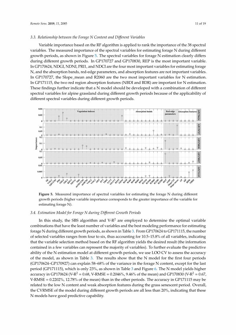
Overall, as the N content decreases, the REP, AMP, and AD present gradually decreasing variationtrends throughout the growth period, as shown in Figure 4. Due to the impacts of spatial heterogeneitybetween different areas, the changes in red region absorption features and red-edge parametersinevitably exhibit a certain degree of fluctuation with changes in the growth period. The above findingsindicate that dynamic changes in the spectral characteristics within the red region during differentgrowth periods may be related to the forage N.


the variation in AD, the REP of the first three periods (GP170624–GP170830) changes slightly; however, it changes significantly in the last three periods (GP170830–GP171115), which may be closely related to the chlorophyll concentration of the forage. Because the chlorophyll has a close relationship with REP, when the grass gradually senesces in the latter three periods, chlorophyll is gradually decomposed and decreases significantly, resulting in significant REP changes. Moreover, the average REP of the different sampling areas in the GP171115 is 694 nm, which may contribute to identifying the growth period of alpine grassland.

Overall, as the N content decreases, the REP, AMP, and AD present gradually decreasing variation trends throughout the growth period, as shown in Figure 4. Due to the impacts of spatial heterogeneity between different areas, the changes in red region absorption features and red-edge parameters inevitably exhibit a certain degree of fluctuation with changes in the growth period. The above findings indicate that dynamic changes in the spectral characteristics within the red region during different growth periods may be related to the forage N.

Figure 4. Changes in the red-edge parameters (REP and AMP) and red region absorption features (AP and AD) in different sampling areas and growth periods. The green dotted line indicates the logarithm fitting models between the N content and corresponding spectrum feature parameters.

3.3. Relationship between the Forage N Content and Different Variables

Variable importance based on the RF algorithm is applied to rank the importance of the 38 spectral variables. The measured importance of the spectral variables for estimating forage N during different growth periods, as shown in Figure 5. The spectral variables for forage N estimation clearly differs during different growth periods. In GP170727 and GP170830, REP is the most important

Figure 4. Changes in the red-edge parameters (REP and AMP) and red region absorption features(AP and AD) in different sampling areas and growth periods. The green dotted line indicates thelogarithm fitting models between the N content and corresponding spectrum feature parameters.

Remote Sens. 2019, 11, 2085 11 of 19

3.3. Relationship between the Forage N Content and Different Variables

Variable importance based on the RF algorithm is applied to rank the importance of the 38 spectralvariables. The measured importance of the spectral variables for estimating forage N during differentgrowth periods, as shown in Figure 5. The spectral variables for forage N estimation clearly differsduring different growth periods. In GP170727 and GP170830, REP is the most important variable.In GP170624, NDGI, NDNI, PRI1, and NDCI are the four most important variables for estimating forageN, and the absorption bands, red-edge parameters, and absorption features are not important variables.In GP170727, the Slope_mean and R2060 are the two most important variables for N estimation.In GP171115, the two red region absorption features (NBDI and BDR) are important for N estimation.These findings further indicate that a N model should be developed with a combination of differentspectral variables for alpine grassland during different growth periods because of the applicability ofdifferent spectral variables during different growth periods.


variable. In GP170624, NDGI, NDNI, PRI1, and NDCI are the four most important variables for estimating forage N, and the absorption bands, red-edge parameters, and absorption features are not important variables. In GP170727, the Slope_mean and R2060 are the two most important variables for N estimation. In GP171115, the two red region absorption features (NBDI and BDR) are important for N estimation. These findings further indicate that a N model should be developed with a combination of different spectral variables for alpine grassland during different growth periods because of the applicability of different spectral variables during different growth periods.

Figure 5. Measured importance of spectral variables for estimating the forage N during different growth periods (higher variable importance corresponds to the greater importance of the variable for estimating forage N).

3.4. Estimation Model for Forage N during Different Growth Periods

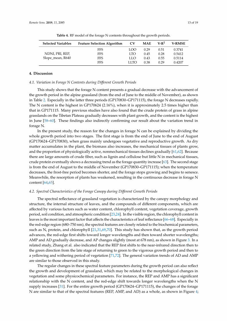
In this study, the SBS algorithm and V-R2 are employed to determine the optimal variable combinations that have the least number of variables and the best modeling performance for estimating forage N during different growth periods, as shown in Table 3. From GP170624 to GP171115, the number of selected variables ranges from four to six, thus accounting for 10.5–15.8% of all variables, indicating that the variable selection method based on the RF algorithm yields the desired result (the information contained in a few variables can represent the majority of variables). To further evaluate the predictive ability of the N estimation model at different growth periods, we use LOO CV to assess the accuracy of the model, as shown in Table 3. The results show that the N model for the first four periods (GP170624–GP170927) can explain 58–68% of the variance in the forage N content, except for the last period (GP171115), which is only 23%, as shown in Table 3 and Figure 6. The N model yields higher accuracy in GP170624 (V-R2 = 0.68, V-RMSE = 0.2046%, 9.46% of the mean) and GP170830 (V-R2 = 0.67, V-RMSE = 0.2202%, 12.78% of the mean) than in the other periods. The accuracy in GP171115 may be related to the low N content and weak absorption features during the grass senescent period. Overall, the CVRMSE of the model during different growth periods are all less than 20%, indicating that these N models have good predictive capability.

Figure 5. Measured importance of spectral variables for estimating the forage N during differentgrowth periods (higher variable importance corresponds to the greater importance of the variable forestimating forage N).

3.4. Estimation Model for Forage N during Different Growth Periods

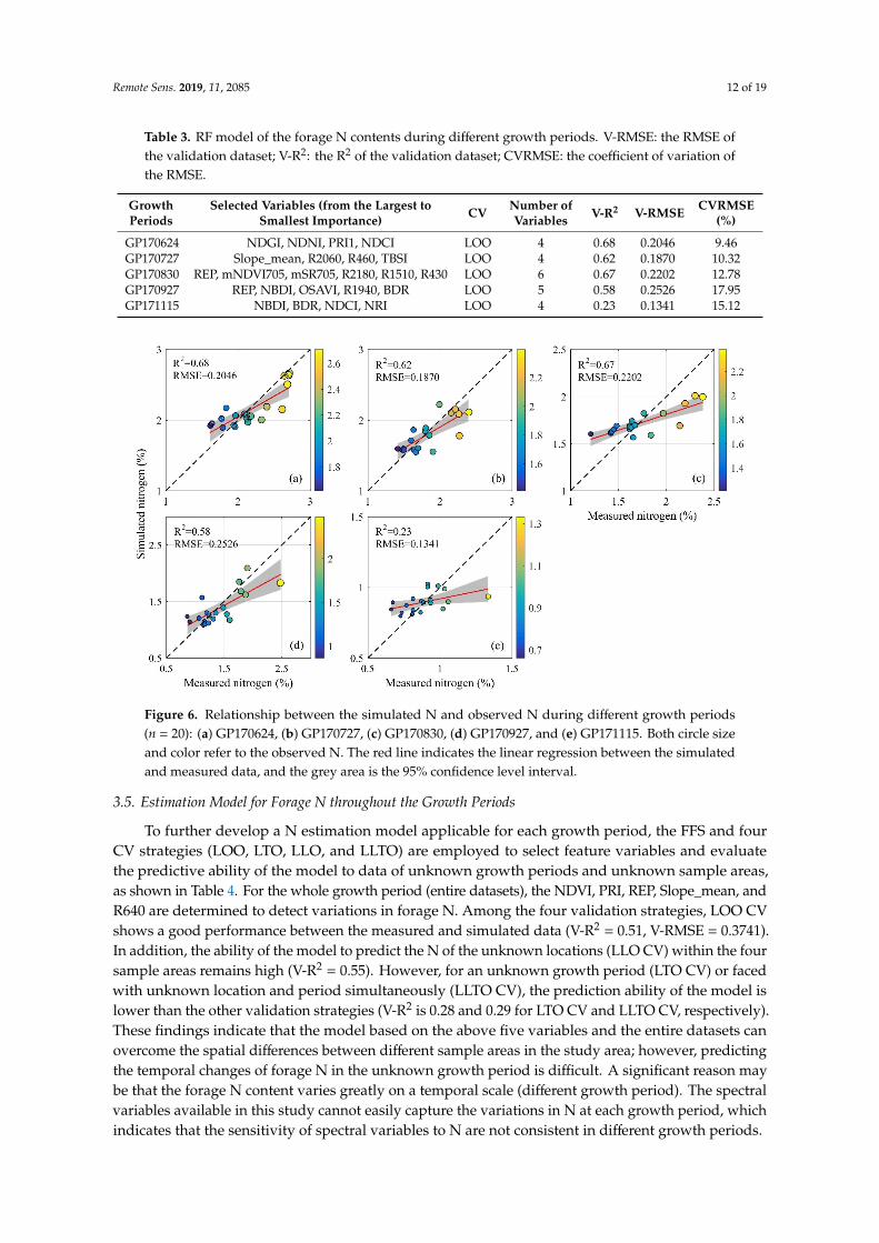
In this study, the SBS algorithm and V-R2 are employed to determine the optimal variablecombinations that have the least number of variables and the best modeling performance for estimatingforage N during different growth periods, as shown in Table 3. From GP170624 to GP171115, the numberof selected variables ranges from four to six, thus accounting for 10.5–15.8% of all variables, indicatingthat the variable selection method based on the RF algorithm yields the desired result (the informationcontained in a few variables can represent the majority of variables). To further evaluate the predictiveability of the N estimation model at different growth periods, we use LOO CV to assess the accuracyof the model, as shown in Table 3. The results show that the N model for the first four periods(GP170624–GP170927) can explain 58–68% of the variance in the forage N content, except for the lastperiod (GP171115), which is only 23%, as shown in Table 3 and Figure 6. The N model yields higheraccuracy in GP170624 (V-R2 = 0.68, V-RMSE = 0.2046%, 9.46% of the mean) and GP170830 (V-R2 = 0.67,V-RMSE = 0.2202%, 12.78% of the mean) than in the other periods. The accuracy in GP171115 may berelated to the low N content and weak absorption features during the grass senescent period. Overall,the CVRMSE of the model during different growth periods are all less than 20%, indicating that theseN models have good predictive capability.

Remote Sens. 2019, 11, 2085 12 of 19

Table 3. RF model of the forage N contents during different growth periods. V-RMSE: the RMSE ofthe validation dataset; V-R2: the R2 of the validation dataset; CVRMSE: the coefficient of variation ofthe RMSE.

GrowthPeriods

Selected Variables (from the Largest toSmallest Importance) CV Number of

Variables V-R2 V-RMSE CVRMSE(%)

GP170624 NDGI, NDNI, PRI1, NDCI LOO 4 0.68 0.2046 9.46GP170727 Slope_mean, R2060, R460, TBSI LOO 4 0.62 0.1870 10.32GP170830 REP, mNDVI705, mSR705, R2180, R1510, R430 LOO 6 0.67 0.2202 12.78GP170927 REP, NBDI, OSAVI, R1940, BDR LOO 5 0.58 0.2526 17.95GP171115 NBDI, BDR, NDCI, NRI LOO 4 0.23 0.1341 15.12


Table 3. RF model of the forage N contents during different growth periods. V-RMSE: the RMSE of the validation dataset; V-R2: the R2 of the validation dataset; CVRMSE: the coefficient of variation of the RMSE.

Growth Periods Selected Variables (from the Largest to Smallest Importance) CV Number of Variables V-R2 V-RMSE CVRMSE (%) GP170624 NDGI, NDNI, PRI1, NDCI LOO 4 0.68 0.2046 9.46 GP170727 Slope_mean, R2060, R460, TBSI LOO 4 0.62 0.1870 10.32 GP170830 REP, mNDVI705, mSR705, R2180, R1510, R430 LOO 6 0.67 0.2202 12.78 GP170927 REP, NBDI, OSAVI, R1940, BDR LOO 5 0.58 0.2526 17.95 GP171115 NBDI, BDR, NDCI, NRI LOO 4 0.23 0.1341 15.12

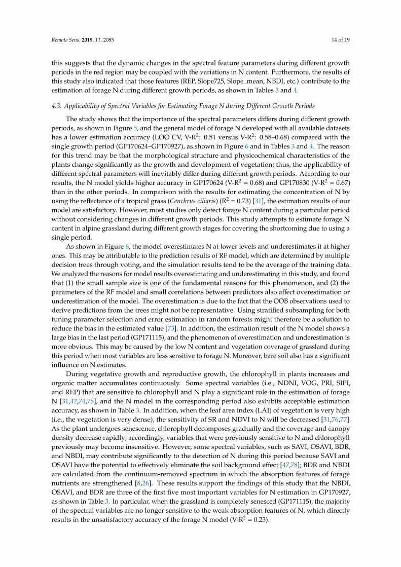
Figure 6. Relationship between the simulated N and observed N during different growth periods (n=20): (a) GP170624, (b) GP170727, (c) GP170830, (d) GP170927, and (e) GP171115. Both circle size and color refer to the observed N. The red line indicates the linear regression between the simulated and measured data, and the grey area is the 95% confidence level interval.

3.5. Estimation Model for Forage N throughout the Growth Periods

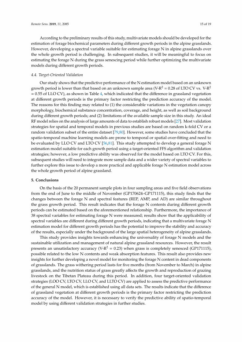
To further develop a N estimation model applicable for each growth period, the FFS and four CV strategies (LOO, LTO, LLO, and LLTO) are employed to select feature variables and evaluate the predictive ability of the model to data of unknown growth periods and unknown sample areas, as shown in Table 4. For the whole growth period (entire datasets), the NDVI, PRI, REP, Slope_mean, and R640 are determined to detect variations in forage N. Among the four validation strategies, LOO CV shows a good performance between the measured and simulated data (V-R2 = 0.51, V-RMSE = 0.3741). In addition, the ability of the model to predict the N of the unknown locations (LLO CV) within the four sample areas remains high (V-R2 = 0.55). However, for an unknown growth period (LTO CV) or faced with unknown location and period simultaneously (LLTO CV), the prediction ability of the model is lower than the other validation strategies (V-R2 is 0.28 and 0.29 for LTO CV and LLTO CV, respectively). These findings indicate that the model based on the above five variables and the entire datasets can overcome the spatial differences between different sample areas in the study area; however, predicting the temporal changes of forage N in the unknown growth period is difficult. A significant reason may be that the forage N content varies greatly on a temporal scale (different growth period). The spectral variables available in this study cannot easily capture the variations in N at each growth period, which indicates that the sensitivity of spectral variables to N are not consistent in different growth periods.

Figure 6. Relationship between the simulated N and observed N during different growth periods(n = 20): (a) GP170624, (b) GP170727, (c) GP170830, (d) GP170927, and (e) GP171115. Both circle sizeand color refer to the observed N. The red line indicates the linear regression between the simulatedand measured data, and the grey area is the 95% confidence level interval.

3.5. Estimation Model for Forage N throughout the Growth Periods

To further develop a N estimation model applicable for each growth period, the FFS and fourCV strategies (LOO, LTO, LLO, and LLTO) are employed to select feature variables and evaluatethe predictive ability of the model to data of unknown growth periods and unknown sample areas,as shown in Table 4. For the whole growth period (entire datasets), the NDVI, PRI, REP, Slope_mean, andR640 are determined to detect variations in forage N. Among the four validation strategies, LOO CVshows a good performance between the measured and simulated data (V-R2 = 0.51, V-RMSE = 0.3741).In addition, the ability of the model to predict the N of the unknown locations (LLO CV) within the foursample areas remains high (V-R2 = 0.55). However, for an unknown growth period (LTO CV) or facedwith unknown location and period simultaneously (LLTO CV), the prediction ability of the model islower than the other validation strategies (V-R2 is 0.28 and 0.29 for LTO CV and LLTO CV, respectively).These findings indicate that the model based on the above five variables and the entire datasets canovercome the spatial differences between different sample areas in the study area; however, predictingthe temporal changes of forage N in the unknown growth period is difficult. A significant reason maybe that the forage N content varies greatly on a temporal scale (different growth period). The spectralvariables available in this study cannot easily capture the variations in N at each growth period, whichindicates that the sensitivity of spectral variables to N are not consistent in different growth periods.

Remote Sens. 2019, 11, 2085 13 of 19

Table 4. RF model of the forage N contents throughout the growth periods.

Selected Variables Feature Selection Algorithm CV MAE V-R2 V-RMSE

NDNI, PRI, REP,Slope_mean, R640

FFS LOO 0.29 0.51 0.3741FFS LTO 0.45 0.28 0.5412FFS LLO 0.43 0.55 0.5114FFS LLTO 0.38 0.29 0.4207

4. Discussion

4.1. Variation in Forage N Contents during Different Growth Periods

This study shows that the forage N content presents a gradual decrease with the advancement ofthe growth period in the alpine grassland (from the end of June to the middle of November), as shownin Table 2. Especially in the latter three periods (GP170830–GP171115), the forage N decreases rapidly.The N content is the highest in GP170624 (2.16%), when it is approximately 2.5 times higher thanthat in GP171115. Many previous studies have also found that the crude protein of grass in alpinegrasslands on the Tibetan Plateau gradually decreases with plant growth, and the content is the highestin June [58–60]. These findings also indirectly confirming our result about the variation trend inforage N.

In the present study, the reason for the changes in forage N can be explained by dividing thewhole growth period into two stages. The first stage is from the end of June to the end of August(GP170624–GP170830), when grass mainly undergoes vegetative and reproductive growth. As drymatter accumulates in the plant, the biomass also increases, the mechanical tissues of plants grow,and the proportion of physiologically active, nonmechanical tissues declines gradually [61,62]. Becausethere are large amounts of crude fiber, such as lignin and cellulose but little N in mechanical tissues,crude protein eventually shows a decreasing trend as the forage quantity increase [63]. The second stageis from the end of August to the middle of November (GP170830–GP171115); when the temperaturedecreases, the frost-free period becomes shorter, and the forage stops growing and begins to senesce.Meanwhile, the resorption of plants has weakened, resulting in the continuous decrease in forage Ncontent [64,65].

4.2. Spectral Characteristics of the Forage Canopy during Different Growth Periods

The spectral reflectance of grassland vegetation is characterized by the canopy morphology andstructure, the internal structure of leaves, and the compounds of different components, which areaffected by various factors such as water content, chlorophyll content, vegetation coverage, growthperiod, soil condition, and atmospheric condition [23,24]. In the visible region, the chlorophyll content inleaves is the most important factor that affects the characteristics of leaf reflectance [66–68]. Especially inthe red-edge region (680–750 nm), the spectral features are closely related to the biochemical parameters,such as N, protein, and chlorophyll [21,31,69,70]. This study has shown that, as the growth periodadvances, the red-edge first shifts toward longer wavelengths and then toward shorter wavelengths;AMP and AD gradually decrease, and AP changes slightly (most at 678 nm), as shown in Figure 3. In arelated study, Zhang et al. also indicated that the REP first shifts to the near-infrared direction then tothe green direction from the late stage of returning to green to the vigorous growth period and then toa yellowing and withering period of vegetation [71,72]. The general variation trends of AD and AMPare similar to those observed in this study.

The regular changes in these spectral feature parameters during the growth period can also reflectthe growth and development of grassland, which may be related to the morphological changes invegetation and some physicochemical parameters. For instance, the REP and AMP has a significantrelationship with the N content, and the red-edge shift towards longer wavelengths when the Nsupply increases [31]. For the entire growth period (GP170624–GP171115), the changes of the forageN are similar to that of the spectral features (REP, AMP, and AD) as a whole, as shown in Figure 4;

Remote Sens. 2019, 11, 2085 14 of 19

this suggests that the dynamic changes in the spectral feature parameters during different growthperiods in the red region may be coupled with the variations in N content. Furthermore, the results ofthis study also indicated that those features (REP, Slope725, Slope_mean, NBDI, etc.) contribute to theestimation of forage N during different growth periods, as shown in Tables 3 and 4.

4.3. Applicability of Spectral Variables for Estimating Forage N during Different Growth Periods

The study shows that the importance of the spectral parameters differs during different growthperiods, as shown in Figure 5, and the general model of forage N developed with all available datasetshas a lower estimation accuracy (LOO CV, V-R2: 0.51 versus V-R2: 0.58–0.68) compared with thesingle growth period (GP170624–GP170927), as shown in Figure 6 and in Tables 3 and 4. The reasonfor this trend may be that the morphological structure and physicochemical characteristics of theplants change significantly as the growth and development of vegetation; thus, the applicability ofdifferent spectral parameters will inevitably differ during different growth periods. According to ourresults, the N model yields higher accuracy in GP170624 (V-R2 = 0.68) and GP170830 (V-R2 = 0.67)than in the other periods. In comparison with the results for estimating the concentration of N byusing the reflectance of a tropical grass (Cenchrus ciliaris) (R2 = 0.73) [31], the estimation results of ourmodel are satisfactory. However, most studies only detect forage N content during a particular periodwithout considering changes in different growth periods. This study attempts to estimate forage Ncontent in alpine grassland during different growth stages for covering the shortcoming due to using asingle period.

As shown in Figure 6, the model overestimates N at lower levels and underestimates it at higherones. This may be attributable to the prediction results of RF model, which are determined by multipledecision trees through voting, and the simulation results tend to be the average of the training data.We analyzed the reasons for model results overestimating and underestimating in this study, and foundthat (1) the small sample size is one of the fundamental reasons for this phenomenon, and (2) theparameters of the RF model and small correlations between predictors also affect overestimation orunderestimation of the model. The overestimation is due to the fact that the OOB observations used toderive predictions from the trees might not be representative. Using stratified subsampling for bothtuning parameter selection and error estimation in random forests might therefore be a solution toreduce the bias in the estimated value [73]. In addition, the estimation result of the N model shows alarge bias in the last period (GP171115), and the phenomenon of overestimation and underestimation ismore obvious. This may be caused by the low N content and vegetation coverage of grassland duringthis period when most variables are less sensitive to forage N. Moreover, bare soil also has a significantinfluence on N estimates.

During vegetative growth and reproductive growth, the chlorophyll in plants increases andorganic matter accumulates continuously. Some spectral variables (i.e., NDNI, VOG, PRI, SIPI,and REP) that are sensitive to chlorophyll and N play a significant role in the estimation of forageN [31,42,74,75], and the N model in the corresponding period also exhibits acceptable estimationaccuracy, as shown in Table 3. In addition, when the leaf area index (LAI) of vegetation is very high(i.e., the vegetation is very dense), the sensitivity of SR and NDVI to N will be decreased [31,76,77].As the plant undergoes senescence, chlorophyll decomposes gradually and the coverage and canopydensity decrease rapidly; accordingly, variables that were previously sensitive to N and chlorophyllpreviously may become insensitive. However, some spectral variables, such as SAVI, OSAVI, BDR,and NBDI, may contribute significantly to the detection of N during this period because SAVI andOSAVI have the potential to effectively eliminate the soil background effect [47,78]; BDR and NBDIare calculated from the continuum-removed spectrum in which the absorption features of foragenutrients are strengthened [8,26]. These results support the findings of this study that the NBDI,OSAVI, and BDR are three of the first five most important variables for N estimation in GP170927,as shown in Table 3. In particular, when the grassland is completely senesced (GP171115), the majorityof the spectral variables are no longer sensitive to the weak absorption features of N, which directlyresults in the unsatisfactory accuracy of the forage N model (V-R2 = 0.23).

Remote Sens. 2019, 11, 2085 15 of 19

According to the preliminary results of this study, multivariate models should be developed for theestimation of forage biochemical parameters during different growth periods in the alpine grasslands.However, developing a spectral variable suitable for estimating forage N in alpine grasslands overthe whole growth period is challenging. In subsequent studies, it will be meaningful to focus onestimating the forage N during the grass senescing period while further optimizing the multivariatemodels during different growth periods.

4.4. Target-Oriented Validation

Our study shows that the predictive performance of the N estimation model based on an unknowngrowth period is lower than that based on an unknown sample area (V-R2 = 0.28 of LTO CV vs. V-R2

= 0.55 of LLO CV), as shown in Table 4, which indicated that the difference in grassland vegetationat different growth periods is the primary factor restricting the prediction accuracy of the model.The reasons for this finding may related to (1) the considerable variations in the vegetation canopymorphology, biochemical substance concentration, coverage, and height, as well as soil backgroundduring different growth periods; and (2) limitations of the available sample size in this study. An idealRF model relies on the analysis of large amounts of data to establish robust models [27]. Most validationstrategies for spatial and temporal models in previous studies are based on random k-fold CV or arandom validation subset of the entire dataset [79,80]. However, some studies have concluded that thespatio-temporal machine learning models are prone to temporal or spatial over-fitting and need tobe evaluated by LLO CV and LTO CV [56,81]. This study attempted to develop a general forage Nestimation model suitable for each growth period using a target-oriented FFS algorithm and validationstrategies; however, a low predictive ability was observed for the model based on LTO CV. For this,subsequent studies will need to integrate more sample data and a wider variety of spectral variables tofurther explore this issue to develop a more practical and applicable forage N estimation model acrossthe whole growth period of alpine grassland.

5. Conclusions

On the basis of the 20 permanent sample plots in four sampling areas and five field observationsfrom the end of June to the middle of November (GP170624–GP171115), this study finds that thechanges between the forage N and spectral features (REP, AMP, and AD) are similar throughoutthe grass growth period. This result indicates that the forage N contents during different growthperiods can be estimated based on the aforementioned relationship. Furthermore, the importance of38 spectral variables for estimating forage N were measured; results show that the applicability ofspectral variables are different during different growth periods, indicating that a multivariate forage Nestimation model for different growth periods has the potential to improve the stability and accuracyof the results, especially under the background of the large spatial heterogeneity of alpine grasslands.

This study provides insights towards enhancing the universality of forage N models and thesustainable utilization and management of natural alpine grassland resources. However, the resultpresents an unsatisfactory accuracy (V-R2 = 0.23) when grass is completely senesced (GP171115),possible related to the low N contents and weak absorption features. This result also provides newinsights for further developing a novel model for monitoring the forage N content in dead componentsof grasslands. The grass withering period lasts for five months (from November to March) in alpinegrasslands, and the nutrition status of grass greatly affects the growth and reproduction of grazinglivestock on the Tibetan Plateau during this period. In addition, four target-oriented validationstrategies (LOO CV, LTO CV, LLO CV, and LLTO CV) are applied to assess the predictive performanceof the general N model, which is established using all data sets. The results indicate that the differenceof grassland vegetation at different growth periods is the primary factor restricting the predictionaccuracy of the model. However, it is necessary to verify the predictive ability of spatio-temporalmodel by using different validation strategies in further studies.

Remote Sens. 2019, 11, 2085 16 of 19

Author Contributions: All authors contributed significantly to this manuscript. J.G. (Jinlong Gao) and T.L.designed this study. J.G. (Jinlong Gao), J.Y., J.G. (Jing Ge), Q.F., C.W., M.H. and J.L. were responsible for the dataprocessing, analysis, and paper writing. H.X. made valuable revisions and editing of the paper.

Funding: This research was funded by the National Natural Science Foundation of China (31672484, 31702175,and 41401472), the Program for Changjiang Scholars and Innovative Research Team in University (IRT_17R50),the National Key Research and Development Program of China project (2017YFC0504801), and the 111 Project(B12002).

Acknowledgments: We acknowledge editors and reviewers for their positive and constructive commentsand suggestions.

Conflicts of Interest: All coauthors declare that there is no conflict of interests.

References

1. He, J.S.; Wang, L.; Flynn, D.F.B.; Wang, X.P.; Ma, W.H.; Fang, J.Y. Leaf nitrogen: Phosphorus stoichiometryacross Chinese grassland biomes. Oecologia 2018, 155, 301–310. [CrossRef]

2. Lu, X.; Yan, Y.; Sun, J.; Zhang, X.K.; Chen, Y.C.; Wang, X.D.; Cheng, G.W. Carbon, nitrogen, and phosphorusstorage in alpine grassland ecosystems of Tibet: Effects of grazing exclusion. Ecol. Evol. 2015, 5, 4492–4504.[CrossRef]

3. Adams, M.A.; Turnbull, T.L.; Sprent, J.I.; Buchmann, N. Legumes are different: Leaf nitrogen, photosynthesis,and water use efficiency. Proc. Natl. Acad. Sci. USA 2016, 113, 4098–4103. [CrossRef]

4. Heckathorn, S.A.; Delucia, E.H.; Zielinski, R.E. The contribution of drought-related decreases in foliarnitrogen concentration to decreases in photosynthetic capacity during and after drought in prairie grasses.Physiol. Plant. 1997, 101, 173–182. [CrossRef]

5. Lu, J.L.; Hu, A.T. Plant Nutriology; Higher Education Press: Beijing, China, 2006.6. Reich, P.B.; Walters, M.B.; Tjoelker, M.G.; Vanderklein, D.; Buschena, C. Photosynthesis and respiration rates

depend on leaf and root morphology and nitrogen concentration in nine boreal tree species differing inrelative growth rate. Funct. Ecol. 2010, 12, 395–405. [CrossRef]

7. Beeri, O.; Phillips, R.; Hendrickson, J.; Frank, A.B.; Kronberg, S. Estimating forage quantity and quality usingaerial hyperspectral imagery for northern mixed-grass prairie. Remote Sens. Environ. 2007, 110, 216–225.[CrossRef]

8. Mutanga, O.; Adam, E.; Adjorlolo, C.; Rahman, E.M.A. Evaluating the robustness of models developed fromfield spectral data in predicting African grass foliar nitrogen concentration using WorldView-2 image as anindependent test dataset. Int. J. Appl. Earth Obs. Geoinf. 2015, 34, 178–187. [CrossRef]

9. Mutanga, O.; Skidmore, A.K.; Prins, H.H.T. Predicting in situ pasture quality in the Kruger National Park,South Africa, using continuum-removed absorption features. Remote Sens. Environ. 2004, 89, 393–408.[CrossRef]

10. Singh, L.; Mutanga, O. Remote sensing of key grassland nutrients using hyperspectral techniques inKwaZulu-Natal, South Africa. J. Appl. Remote Sens. 2017, 11, 036005. [CrossRef]

11. Shoko, C.; Mutanga, O.; Dube, T. Progress in the remote sensing of C3 and C4 grass species abovegroundbiomass over time and space. ISPRS J. Photogramm. Remote Sens. 2016, 120, 13–24. [CrossRef]

12. Adjorlolo, C.; Cho, M.A.; Mutanga, O.; Ismail, R. Optimizing spectral resolutions for the classification ofC3 and C4 grass species, using wavelengths of known absorption features. J. Appl. Remote Sens. 2012, 6,217–224. [CrossRef]

13. Mccann, C.; Repasky, K.S.; Lawrence, R.; Powell, S. Multi-temporal mesoscale hyperspectral data of mixedagricultural and grassland regions for anomaly detection. ISPRS J. Photogramm. Remote Sens. 2017, 131,121–133. [CrossRef]

14. Ramoelo, A.; Skidmore, A.K.; Cho, M.A.; Mathieu, R.; Heitkönig, I.M.A.; Dudeni-Tlhone, N.; Schlerf, M.;Prins, H.H.T. Non-linear partial least square regression increases the estimation accuracy of grass nitrogenand phosphorus using in situ hyperspectral and environmental data. ISPRS J. Photogramm. Remote Sens.2013, 82, 27–40. [CrossRef]

15. Ramoelo, A.A. Monitoring grass nutrients and biomass as indicators of rangeland quality and quantity usingrandom forest modelling and WorldView-2 data. Int. J. Appl. Earth Obs. Geoinf. 2015, 43, 43–54. [CrossRef]

16. Curran, P.J. Remote sensing of foliar chemistry. Remote Sens. Environ. 1989, 30, 271–278. [CrossRef]

http://dx.doi.org/10.1007/s00442-007-0912-y

http://dx.doi.org/10.1002/ece3.1732

http://dx.doi.org/10.1073/pnas.1523936113

http://dx.doi.org/10.1111/j.1399-3054.1997.tb01834.x

http://dx.doi.org/10.1046/j.1365-2435.1998.00209.x

http://dx.doi.org/10.1016/j.rse.2007.02.027

http://dx.doi.org/10.1016/j.jag.2014.08.008


http://dx.doi.org/10.1117/1.JRS.11.036005

http://dx.doi.org/10.1016/j.isprsjprs.2016.08.001

http://dx.doi.org/10.1117/1.JRS.6.063560




http://dx.doi.org/10.1016/0034-4257(89)90069-2

Remote Sens. 2019, 11, 2085 17 of 19

17. Knox, N. Observing Temporal and Spatial Variability of Forage Quality. Ph.D. Thesis, Faculty Geo-InformationScience and Earth Observation and Twente University, Enschede, The Netherlands, 2010.

18. Schlerf, M.; Atzberger, C.; Hill, J.; Buddenbaum, H.; Werner, W.; Schüler, G. Retrieval of chlorophyll andnitrogen in Norway spruce (Picea abies L. Karst.) using imaging spectroscopy. Int. J. Appl. Earth Obs. Geoinf.2010, 12, 17–26. [CrossRef]

19. Skidmore, A.K.; Ferwerda, J.G.; Mutanga, O.; Van Wieren, S.E.; Peel, M.; Grant, R.C.; Prins, H.H.T.; Balcik, F.B.;Venus, V. Forage quality of savannas–simultaneously mapping foliar protein and polyphenols for trees andgrass using hyperspectral imagery. Remote Sens. Environ. 2010, 114, 64–72. [CrossRef]

20. Mutanga, O.; Skidmore, A.K. Red edge shift and biochemical content in grass canopies. ISPRS J. Photogramm.Remote Sens. 2007, 62, 34–42. [CrossRef]

21. Clevers, J.G.P.W.; Gitelson, A.A. Remote estimation of crop and grass chlorophyll and nitrogen content usingred-edge bands on Sentinel-2 and -3. Int. J. Appl. Earth Obs. Geoinf. 2013, 23, 344–351. [CrossRef]

22. Lin, D.; Wei, G.; Jian, Y. Application of spectral indices and reflectance spectrum on leaf nitrogen contentanalysis derived from hyperspectral LiDAR data. Opt. Laser Technol. 2018, 107, 372–379.

23. Choubey, V.K.; Choubey, R. Spectral reflectance, growth and chlorophyll relationships for rice crop in asemi-arid region of India. Water Resour. Manag. 1999, 13, 73–84. [CrossRef]

24. Sims, D.A.; Gamon, J.A. Relationships between leaf pigment content and spectral reflectance across awide range of species, leaf structures and developmental stages. Remote Sens. Environ. 2002, 81, 337–354.[CrossRef]

25. Ramoelo, A.; Cho, M.A.; Madonsela, S.; Mathieu, R.; Korchove, R.V.D.; Kaszta, Z.; Wolf, E. A potential tomonitor nutrients as an indicator of rangeland quality using space borne remote sensing. IOP Conf. Ser.Earth Environ. Sci. 2014, 18, 012094. [CrossRef]

26. Gong, Z.; Kawamura, K.; Ishikawa, N.; Inaba, M.; Alateng, D. Estimation of herbage biomass and nutritivestatus using band depth features with partial least squares regression in Inner Mongolia grassland, China.Grassl. Sci. 2016, 62, 45–54. [CrossRef]

27. Breiman, L. Random forests. Mach. Learn. 2001, 45, 5–32. [CrossRef]28. Mutanga, O.; Adam, E.; Cho, M.A. High density biomass estimation for wetland vegetation using WorldView-2

imagery and random forest regression algorithm. Int. J. Appl. Earth Obs. Geoinf. 2012, 18, 399–406. [CrossRef]29. Singh, L.; Mutanga, O.; Mafongoya, P.; Peerbhay, K.Y. Multispectral mapping of key grassland nutrients in

KwaZulu-Natal, South Africa. J. Spat. Sci. 2018, 63, 155–172. [CrossRef]30. Gao, J.L.; Meng, B.P.; Liang, T.G.; Feng, Q.S.; Ge, J.; Yin, J.P.; Wu, C.X.; Cui, X.; Hou, M.J.; Liu, J.; et al.

Modeling alpine grassland forage phosphorus based on hyperspectral remote sensing and a multi-factormachine learning algorithm in the east of Tibetan Plateau, China. ISPRS J. Photogramm. Remote Sens. 2019,147, 104–117. [CrossRef]

31. Mutanga, O. Hyperspectral Remote Sensing of Tropical Grass Quality and Quantity. Ph.D. Thesis,International Institute for Geoinformation Science and Earth Observation and Wageningen University,Wageningen, The Netherlands, 2004.

32. Horler, D.N.H.; Dockray, M.; Barber, J. The red edge of plant leaf reflectance. Int. J. Remote Sens. 1983, 4,273–288. [CrossRef]

33. Guo, C.F.; Guo, X.Y. Estimating leaf chlorophyll and nitrogen content of wetland emergent plants usinghyperspectral data in the visible domain. Spectrosc. Lett. 2016, 49, 180–187. [CrossRef]

34. Jordan, C.F. Derivation of leaf area index from quality of light on the forest floor. Ecology 1969, 50, 663–666.[CrossRef]

35. Gitelson, A.A.; Merzlyak, M.N. Spectral reflectance changes associated with autumn senescence ofAesculus hippocastanum L. and Acer platanoides L. leaves. Spectral Features and Relation to ChlorophyllEstimation. J. Plant Physiol. 1994, 143, 286–292. [CrossRef]

36. Datt, B. A new reflectance index for remote sensing of chlorophyll content in higher plants: Tests usingEucalyptus leaves. J. Plant Physiol. 1991, 154, 30–36. [CrossRef]

37. Clevers, J.G.P.W. Imaging Spectrometry in Agriculture—Plant Vitality and Yield Indicators Imaging Spectrometry—ATool for Environmental Observations; Springer: Dordrecht, The Netherlands, 1994; pp. 193–219.

38. Vogelmann, J.E.; Rock, B.N.; Moss, D.M. Red edge spectral measurements from sugar maple leaves. Int. J.Remote Sens. 1993, 14, 1563–1575. [CrossRef]





http://dx.doi.org/10.1023/A:1008056400348

http://dx.doi.org/10.1016/S0034-4257(02)00010-X

http://dx.doi.org/10.1088/1755-1315/18/1/012094

http://dx.doi.org/10.1111/grs.12112

http://dx.doi.org/10.1023/A:1010933404324


http://dx.doi.org/10.1080/14498596.2017.1341352


http://dx.doi.org/10.1080/01431168308948546

http://dx.doi.org/10.1080/00387010.2015.1118126

http://dx.doi.org/10.2307/1936256

http://dx.doi.org/10.1016/S0176-1617(11)81633-0

http://dx.doi.org/10.1016/S0176-1617(99)80314-9

http://dx.doi.org/10.1080/01431169308953986

Remote Sens. 2019, 11, 2085 18 of 19

39. Fourty, T.; Baret, F.; Jacquemoud, S. Leaf optical properties with explicit description of its biochemicalcomposition: Direct and inverse problems. Remote Sens. Environ. 1996, 56, 104–117. [CrossRef]

40. Serrano, L.; Peñuelas, J.; Ustin, S.L. Remote sensing of nitrogen and lignin in Mediterranean vegetation fromAVIRIS data: Decomposing biochemical from structural signals. Remote Sens. Environ. 2002, 81, 355–364.[CrossRef]

41. Gamon, J.A.; Penuelas, J.; Field, C.B. A narrow-waveband spectral index that tracks diurnal changes inphotosynthetic efficiency. Remote Sens. Environ. 1992, 41, 35–44. [CrossRef]

42. Penuelas, J.; Baret, F.; Filella, I. Semiempirical indexes to assess carotenoids chlorophyll-a ratio from leafspectral reflectance. Photosynthetica 1995, 31, 221–230.

43. Rondeaux, G.; Steven, M.; Baret, F. Optimization of soil-adjusted vegetation indices. Remote Sens. Environ.1996, 55, 95–107. [CrossRef]

44. Richardson, A.J.; Wiegand, C.L. Distinguishing vegetation from soil background information (by graymapping of Landsat MSS data). Photogramm. Eng. Remote Sens. 1997, 43, 1541–1552.

45. Gitelson, A.A.; Merzlyak, M.N. Signature analysis of leaf reflectance spectra: Algorithm development forremote sensing of chlorophyll. J. Plant Physiol. 1996, 148, 494–500. [CrossRef]

46. Marshak, A.; Knyazikhin, Y.; Davis, A.; Wiscombe, W.; Pilewskie, P. Cloud-vegetation interaction: Use ofnormalized difference cloud index for estimation of cloud optical thickness. Geophys. Res. Lett. 2000, 27,1695–1698. [CrossRef]

47. Huete, A.R. A soil-adjusted vegetation index (SAVI). Remote Sens. Environ. 1988, 25, 295–309. [CrossRef]48. Roujean, J.L.; Breon, F.M. Estimating PAR absorbed by vegetation from bidirectional reflectance measurements.

Remote Sens. Environ. 1995, 51, 375–384. [CrossRef]49. Huete, A.; Didan, K.; Miura, T.; Rodriguez, E.P.; Gao, X.; Ferreira, L.G. Overview of the radiometric

and biophysical performance of the MODIS vegetation indices. Remote Sens. Environ. 2002, 83, 195–213.[CrossRef]

50. Schleicher, T.D.; Bausch, W.C.; Delgado, J.A.; Ayers, P.D. Evaluation and Refinement of the NitrogenReflectance Index (NRI) for Site-Specific Fertilizer Management. In ASAE Annual International Meeting Report;American Society of Agricultural and Biological Engineers: St Joseph, MI, USA, 1998.

51. Tian, Y.C.; Gu, K.J.; Chu, X.; Yao, X.; Cao, W.X.; Zhu, Y. Comparison of different hyperspectral vegetationindices for canopy leaf nitrogen concentration estimation in rice. Plant Soil 2014, 376, 193–209. [CrossRef]

52. Kumar, L.; Schmidt, K.S.; Dury, S.; Skidmore, A.K. Imaging spectroscopy and vegetation science. ImagingSpectrom. Basic Princ. Prospect. Appl. 2001, 4, 111–155.

53. Mutanga, O.; Skidmore, A.K.; Kumar, L.; Ferwerda, J. Estimating tropical pasture quality at canopy levelusing band depth analysis with continuum removal in the visible domain. Int. J. Remote Sens. 2005, 26,1093–1108. [CrossRef]

54. Han, Z.Y.; Zhu, X.C.; Fang, X.Y.; Wang, Z.Y.; Wang, L.; Zhao, G.X.; Jiang, Y.M. Hyperspectral estimation ofapple tree canopy LAI based on SVM and RF regression. Spectrosc. Spectr. Anal. 2016, 36, 800–805.

55. Lebedev, A.; Westman, E.; Van Westen, G.; Kramberger, M.; Lundervold, A.; Aarsland, D.; Soininen, H.;Kłoszewska, I.; Mecocci, P.; Tsolaki, M. Random Forest ensembles for detection and prediction of Alzheimer’sdisease with a good between-cohort robustness. Neuroimage Clin. 2014, 6, 115–125. [CrossRef]

56. Meyer, H.; Reudenbach, C.; Hengl, T.; Katurji, M.; Nauss, T. Improving performance of spatio-temporalmachine learning models using forward feature selection and target-oriented validation. Environ. Model.Softw. 2018, 101, 1–9. [CrossRef]

57. Efron, B.; Gong, G. A leisurely look at the bootstrap, the jackknife, and cross-validation. Am. Stat. 1983, 37,36–48.

58. Zhao, Z.; Wang, A.L.; Ma, H.S.; Song, H.Q. Studies on dynamics monitor and sustainable development ineastern edge of Qinghai-Tibetan alpine grassland (III Seasonal variational dynamics of nutrional contents ofthe predominant plants on 8 main grassland types). Pratacult. Sci. 2002, 19, 5–9.

59. Liang, J.Y.; Jiao, T.; Wu, J.P.; Gong, X.Y.; Du, W.H.; Liu, H.B.; Xiao, Y.M. The relationship between seasonalforage digestibility and forage nutritive value in different grazing pastures. Acta Pratacult. Sin. 2015, 24,108–115.

60. Zhou, H.J.; Mao, Z.X.; Huang, D.J.; Fu, H. Analysis on nutritional quality of Elymus nutans among differentpopulations on Qinghai-Tibet Plateau. Pratacult. Sci. 2011, 28, 1198–1202.

http://dx.doi.org/10.1016/0034-4257(95)00234-0

http://dx.doi.org/10.1016/S0034-4257(02)00011-1

http://dx.doi.org/10.1016/0034-4257(92)90059-S

http://dx.doi.org/10.1016/0034-4257(95)00186-7

http://dx.doi.org/10.1016/S0176-1617(96)80284-7

http://dx.doi.org/10.1029/1999GL010993

http://dx.doi.org/10.1016/0034-4257(88)90106-X

http://dx.doi.org/10.1016/0034-4257(94)00114-3

http://dx.doi.org/10.1016/S0034-4257(02)00096-2

http://dx.doi.org/10.1007/s11104-013-1937-0

http://dx.doi.org/10.1080/01431160512331326738

http://dx.doi.org/10.1016/j.nicl.2014.08.023

http://dx.doi.org/10.1016/j.envsoft.2017.12.001

Remote Sens. 2019, 11, 2085 19 of 19

61. Niklas, K.J. Plant allometry, leaf nitrogen and phosphorus stoichiometry, and interspecific trends in annualgrowth rates. Ann. Bot. 2005, 97, 155–163. [CrossRef] [PubMed]

62. Niklas, K.J.; Owens, T.; Reich, P.B.; Cobb, E.D. Nitrogen/phosphorus leaf stoichiometry and the scaling ofplant growth. Ecol. Lett. 2005, 8, 636–642. [CrossRef]

63. Shi, Y.; Ma, Y.L.; Ma, W.H.; Liang, C.Z.; Zhao, X.Q.; Fang, J.Y.; He, J.S. Large scale patterns of forage yield andquality across Chinese grasslands. Chin. Sci. Bull. 2013, 58, 1187–1199. [CrossRef]

64. Huang, J.Y.; Zhu, X.G.; Yuan, Z.Y.; Song, S.H.; Li, X.; Li, L.H. Changes in nitrogen resorption traits of sixtemperate grassland species along a multi-level N addition gradient. Plant Soil 2008, 306, 149–158. [CrossRef]

65. Li, L.; Gao, X.P.; Li, X.Y.; Lin, L.S.; Zeng, F.J.; Gui, D.W.; Lu, Y. Nitrogen (N) and phosphorus (P) resorptionof two dominant alpine perennial grass species in response to contrasting N and P availability. Environ.Exp. Bot. 2016, 127, 37–44. [CrossRef]

66. Gitelson, A.A.; Gritz, Y.; Merzlyak, M.N. Relationships between leaf chlorophyll content and spectralreflectance and algorithms for non-destructive chlorophyll assessment in higher plant leaves. J. Plant Physiol.2003, 160, 271–282. [CrossRef] [PubMed]

67. Feng, W. Monitoring Nitrogen Status and Growth Characters with Hyperspectral Remote Sensing in Wheat.Ph.D. Thesis, Nanjing Agriculture University, Nanjing, China, 2007.

68. Yoder, B.J.; Pettigrew-Crosby, R.E. Predicting nitrogen and chlorophyll content and concentrations fromreflectance spectra (400–2500 nm) at leaf and canopy scales. Remote Sens. Environ. 1995, 53, 199–211.[CrossRef]

69. Filella, I.; Penuelas, J. The red edge position and shape as indicators of plant chlorophyll content, biomassand hydric status. Int. J. Remote Sens. 1994, 15, 1459–1470. [CrossRef]

70. Sibanda, M.; Mutanga, O.; Rouget, M. Testing the capabilities of the new WorldView-3 space-borne sensor’sred-edge spectral band in discriminating and mapping complex grassland management treatments. Int. J.Remote Sens. 2017, 38, 1–22. [CrossRef]

71. Zhang, F.L.; Yin, Q.; Kuang, D.B.; Li, F.X.; Zhou, B.R. Analysis of time series spectrum feature parametersderived from dominant natural grasslands in the region around Qinghai lake. Acta Ecol. Sin. 2005, 25,3155–3160.

72. Zhang, F.L.; Yin, Q.; Kuang, D.B.; Li, F.X.; Zhou, B.R. Analysis of a spectral experiment conducted throughthe growth period of the main grassland types found in the region around Qinghai Lake. Acta Pratacult. Sin.2006, 15, 42–47.

73. Janitza, S.; Hornung, R. On the overestimation of random forest’s out-of-bag error. PLoS ONE 2018, 13,e0201904. [CrossRef]

74. Penuelas, J.; Gamon, J.A.; Freeden, A.L.; Merino, J.; Field, C. Reflectance indices associated with physiologicalchanges in nitrogen and water-limited sunflower leaves. Remote Sens. Environ. 1994, 48, 135–146. [CrossRef]

75. Jago, R.A.; Cutler, M.E.J.; Curran, P.J. Estimating canopy chlorophyll concentration from field and airbornespectra. Remote Sens. Environ. 1999, 68, 217–224. [CrossRef]

76. Sellers, P.J. Canopy reflectance, photosynthesis and transpiration. Int. J. Remote Sens. 1985, 6, 1335–1372.[CrossRef]

77. Thenkabail, P.S.; Smith, R.B.; De Pauw, E. Hyperspectral vegetation indices and their relationships withagricultural crop characteristics. Remote Sens. Environ. 2000, 71, 158–182. [CrossRef]

78. Hatfield, J.L.; Prueger, J.H. Value of using different vegetative indices to quantify agricultural cropcharacteristics at different growth stages under varying management practices. Remote Sens. 2010, 2,562–578. [CrossRef]

79. Ke, Y.; Im, J.; Park, S.; Gong, H. Downscaling of MODIS one kilometer evapotranspiration using Landsat-8data and machine learning approaches. Remote Sens. 2016, 8, 215. [CrossRef]

80. Ludwig, A.; Meyer, H.; Nauss, T. Automatic classification of Google Earth images for a larger scale monitoringof bush encroachment in South Africa. Int. J. Appl. Earth Obs. Geoinf. 2016, 50, 89–94. [CrossRef]

81. Gudmundsson, L.; Seneviratne, S.I. Towards observation-based gridded runoff estimates for Europe.Hydrol. Earth Syst. Sci. 2015, 19, 2859–2879. [CrossRef]

© 2019 by the authors. Licensee MDPI, Basel, Switzerland. This article is an open accessarticle distributed under the terms and conditions of the Creative Commons Attribution(CC BY) license (http://creativecommons.org/licenses/by/4.0/).

http://dx.doi.org/10.1093/aob/mcj021

http://www.ncbi.nlm.nih.gov/pubmed/16287903

http://dx.doi.org/10.1111/j.1461-0248.2005.00759.x

http://dx.doi.org/10.1007/s11434-012-5493-4

http://dx.doi.org/10.1007/s11104-008-9565-9

http://dx.doi.org/10.1016/j.envexpbot.2016.03.008

http://dx.doi.org/10.1078/0176-1617-00887

http://www.ncbi.nlm.nih.gov/pubmed/12749084

http://dx.doi.org/10.1016/0034-4257(95)00135-N

http://dx.doi.org/10.1080/01431169408954177

http://dx.doi.org/10.1080/01431161.2016.1259678

http://dx.doi.org/10.1371/journal.pone.0201904

http://dx.doi.org/10.1016/0034-4257(94)90136-8

http://dx.doi.org/10.1016/S0034-4257(98)00113-8

http://dx.doi.org/10.1080/01431168508948283

http://dx.doi.org/10.1016/S0034-4257(99)00067-X

http://dx.doi.org/10.3390/rs2020562

http://dx.doi.org/10.3390/rs8030215


http://dx.doi.org/10.5194/hess-19-2859-2015

http://creativecommons.org/

http://creativecommons.org/licenses/by/4.0/.

Documents

Estimation of Alpine Grassland Forage Nitrogen ... - MDPI