Res. Popul. Ecol. (1990)32, 151--171. ~) by the Society of Population Ecology

E S T I M A T I O N OF C O N T E M P O R A N E O U S M O R T A L I T Y FACTORS

John P. BUONACCORSI* and Joseph S. ELKINTON**

*Department of Mathematics and Statistics, University of Massachusetts, Amherst, Massachusetts 01003, U.S.A.

**Department of Entomology, University of Massachusetts, Amherst, Massachusetts 01003, U.S.A.

INTRODUCTION

Methods for quantification of mortality and construction of life tables for animal

populations were pioneered by Deevy (1947) and extended by Morris (1959) and

Varley and Gradwell (1960) to insect populations with discrete generations. The most

frequent measure of mortality calculated from such life tables is the stage specific or ap-

parent mortality which is defined as the proportion of those hosts that entered a par-

ticular host stage (larval or pupal stage for instance) that are attacked and killed by a

specific agent. However, difficulties arise when more than one agent act contem-

poraneously within a stage. The sum of stage specific mortalities from all contem-

poraneous mortalities within a stage is equal to the total mortality in that stage. The

problem is that the changes in size of the specific mortality will influence the propor-

tion killed by other contemporaneous agents without changing the impact of those lat-

ter agents on the resulting proportion surviving to the end of the generation. Royama

(1981) argued that the problem could be solved if mortality was expressed as the

marginal probabilities of dying (herinafter termed the marginal attack rates) from each

factor. The product of the marginal survivorships (1-marginal attack rate) of all con-

temporaneous factors acting during any particular life stage is equal to the total sur-

vivorship during that stage. The marginal attack rate is typically unaffected by other

sources of mortality and represents the best measure of the impact of a particular mor-

tality agent on its host population. The marginal attack rate can be converted directly

into a k-value (sensu Varley and Gradwell, 1960). It differs from the proportion that

are observed to die from that factor because some individuals that would have died

from that factor during the life stage die from other causes beforehand. In many

studies, the impact of parasitoids or disease agents are measured by collecting hosts

and rearing them to determine what proportion die from disease or from parasitoid

death. The problem faced by researchers who employ such techniques is to estimate

the marginal attack rates from the observed proportions dying.

There are two main issues not fully resolved in the work of Royarna (1981) which

are the subject of this paper. The first has to do with obtaining solutions for the

marginal attack rates given observed proportions dying. This includes the issues of

152

numerical methods to be used and the underlying effects of assumptions about internal

competition among factors. The second major issue is one of carrying out statistical in-

ference from the observed death rates. Usually one has observed death rates from the

field which are used to estimate the marginal attack rates. These are of course subject

to sampling error and one would like to determine appropriate standard errors to at-

tach to these, obtain confidence intervals and test various hypotheses. We will first

treat the problem of solving for the attack rates and then address the statistical issues.

Converting from mortality rates to k-values is also considered.

SOLVING FOR Two FACTORS

Suppose there are two factors A and B that affect a particular life stage or age inter-

val of a population. For instance, suppose we are studying an insect host attacked

during a given life stage or age interval by two parasitoids A and B. If hosts were

collected from the population, we could determine the proportion parasitized either

by dissecting the hosts to look for immature parasitoids or rearing them until adult

parasitoids emerged. What we would like to estimate is the proportion of those hosts

that entered the stage that were attacked by each agent. This proportion is typically

different from the proportion that are present in a given sample due to, among other

things, the phenology of parasitoid oviposition and subsequent adult death (Van

Driesche 1983). However, to illustrate our point we begin by making the following

simple assumptions;

A1. Attacks by A and B are independent, meaning that the probability of attack

by either parasitoid is not influenced by the presence of the other species within the

host. In many host/parasitoid systems, this assumption is not tenable.

A2. A period of time exists during the age interval during which all attacks by A

and B were complete and no death of A and B from the parasitized hosts had occur-

red. A single sample taken at this point thus reflects all hosts that would be attacked

by A or B during the age interval. Otherwise, one would be forced to engage in the

complex procedures for converting sample percentage parasitism into stage specific

values as discussed by Van Driesche (1983) or Southwood (1978). These issues are

beyond the scope of this manuscript.

A3. Death is scored by collecting hosts and rearing them to determine the pro-

portion of hosts from which A or B emerge. In many cases rearing is much easier than

the alternative of dissecting the hosts.

In general, when we speak of a factor emerging, we mean that factor has been

designated as a cause of death for the particular host.

We denote the various combinations for the occurrence of the factors and the

153

sssociated probabilities as follows.

B present B absent

A Present mAB rnAB' mA A Absen ma'~ rnA'B' ran'

?n B ?FtB'

For example, mAB represents the probabili ty that a host has been attacked by both

A and B. Note that ma (=maB+m.4B') and mB (----ma~+mA'~) are the marginal pro-

babilities of attack by A and B respectively. A consequence of the independence

assumption (A1) is that mAB = m a Xml~ with similar factorizations holding for the other

cells. This fac t is crucial in our development.

As noted earlier, the observed death rates are not the same as the marginal attack

rates, since when A and B are both present, both do not necessarily emerge. Pro-

cedures to determine the attack rates from the observed death rates vary, depending on

what assumptions are made regarding death once the agent(s) are present.

Case I: One Factor Emerging

We consider first the case in which at most a single factor is at tr ibuted as the cause

of death. In addition to our earlier assumptions, we assume

A4. Hosts that are attacked by both A and B die from either A or B but not

both. None of the hosts attacked by A or B die without A or B emerging from them.

Tha t is if A is present alone, then A will emerge and similarly for B.

A5. There is some fixed probabili ty c that hosts attacked by both A and B yield A

and, because of assumption 4, probabili ty ( l - - c ) that such hosts yield B.

Let dA=probabil i ty that factor A emerges and dB=probabil i ty that B emerges

denote the death rates due to A and B respectively. It can be shown (see equations

(12) and (13) in Royama (1981)) that under the stated assumptions,

d.4=mA+m,4mB(c--1) and dB=mB--cmAmB. (1)

It can be shown that for a set of death rates (i.e., da and d8 each between 0 and 1,

and dA +dB <-- 1) there is a unique set of marginal attack r a t e s (mA and mB, each between

0 and 1) such that the equations in (1) are satisfied. Assuming 0 < c < 1, the unique

acceptable solution to (1) is

ma=(b--(b2--4cd.4)x/2)/2c and mB=ds/(1--cmA) (2)

where b=c(da+dB)+l-dB. This result is obtained by showing that (1) leads to

solving a quadratic equation for mA with the root given above always being between 0

and 1 while the other root is always greater than 1 (and hence is not acceptable for ma).

In the case where da+dB = 1 either rna, ms or both will equal 1.

154

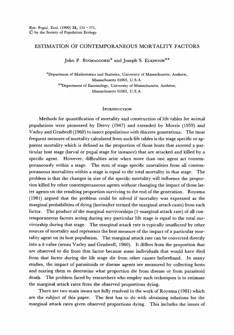
Figure 1 provides solutions for the marginal attack rates for four sets of death

rates, illustrating how the attack rates depend on the choice of the compet i t ion pro-

bability c. For two cases, the solution for the marginal attack rates is relatively insen-

sitive to the value ofc . However , in the other two cases, the value o f t is important.

Analytically, it can be shown that mA decreases as c increases. Hence the maximum value for mA is dA/(l --dB) which occurs at c = 0 and the m i n i m u m value is dA which oc-

curs when c = 1. O f course, the latter result is expected, since if c - -1 , we always see

factor A when it is present and hence the observed death rate is the same as the

marginal attack rate. Similary, the solution for ms has a m i n i m u m value ofdB at c = 0

and a m a x i m u m value of dJ(1 -dA) at c = 1. So even without any knowledge of c, it is

possible to bound the attack rates. It is obvious that the attack rate for a factor is at

least as big as the corresponding death rate.

Carey (1989) proposes an analogous set o f equations and solution but does not

-<

1,0

,9

,8

.7

.6

.5

.4

.3

.2

.1

.0

A 1.0

-9 t B ,-.'""' " ' " ........ . ............................... .B. . .....................

i6 "" ' 5

FACTOR A

- FACTOR B

'.3 -~ '-~ ',6 '.7 "8 '.9 1.0 .o h .~ .o '., '.= :3 '., '.5 ~ '.~ \8 '., ,.o

. 4 �9

.3

.2

. t

,O

<~

Fig. I.

1.0

V9

.8

.7

.6

.5

.4

.3

.2

.I

.0

C . J D

.6 "1

. 4

.3

,2 4 ....................... 2 ................... !

Plots of solutions for marginal attack rates as a function of competit ion probability c, for the two factor/one winner setting, Each of the four plots corresponds to a set of death rates. A; dA=.4, ds----.4 , B; da----.3, ds=.6, C; da = .8, d~=.05, D; da=.2, dn=.2.

.......................................................................... "~ ' "" ' " ' " ' " ' " .1

1 . o ~ . , - F - , , �9 0 , �9

.o '.! ;2 :.t ',4 ;.5 "6 1,7 ",8 '.9 L 0 .0 .I ,2 , .3 .4 .5 .6 .7 .8 ",9 1.0

c c

155

specifically identify the competition probabili ty c for this problem. In order to obtain

a solution he makes the assumption that the ratio of death rates is equal to the ratio of

marginal attack rates; da/dB=ma/mB. Substi tuting the expressions for dA and de from

(1), this assumption implies

mA + mAmB(c -- 1 ) _ mA mB-- cmamB mB '

which leads to c = mB/(mA + roB). That is, c (the probability that A emerges from hosts

parasitized by A and B) is proportional to the marginal attack rate for B. As mB becomes large relative to mA, a larger proportion of the individuals attacked by both

must yield A instead of B. For example, with marginal attack rates of .3 for A and .6

for B, Carey 's assumption implies that the probabili ty that A wins when the two com-

pete is 0.667. We believe that it is more reasonable to assume that either that c = .5 or

that c is proportional to the marginal attack rate for A, rather than B. The latter situa-

tion might arise under the condition of "first one in wins", assuming that both agents

have the same temporal distribution of attacks over the stage or age interval. We can

think of no reason why c should be proportional to the marginal attack rate for B.

Case II: Zero, One or Two Factors Emerging

We generalize now to the case where each host can yield 0, 1 or 2 factors. Let

dA and dB be as defined previously and let dab be the proport ion with both A and B

emerging. This setting clearly requires a more elaborate set of competition probabil-

ities. Let

c(A [A)=P(A emerges when A only is present)

c(B[B) = P(B emerges when B only is present)

c(A IAB)=P(A alone emerges when both A and B are present)

c(B ]AB)=P(B alone emerges when both A and B are present)

c(AB[AB)=P(A and B both emerge when both A and B are present).

Retaining our assumptions 1-3, the following relationships are obtained:

dA=ma(1 --mB) c(A [A)+mamB c(A [AB) (3)

dB= mB(1 -- mA) c( B [ A ) + mAmB c( B MB) (4)

dab = rnamB c(AB lAB). ( 5 )

Equations (14) through (17) of Royama (1981) represent a special case of the

above in which c(A [A) and c(B[B) both equal 1 and c(A [AB)+c(B [AB)+c(ABIAB) = 1. For simplicity, we refer to this as the Royama case.

Care must be taken in trying to solve for the attack rates given the death rates. In

fact, a given set of death rates limits rather severely what competit ion probabilities can

be present. We illustrate with the Royama case, where for convenience we write ca for

156

c(A [AB) , CB for c ( B [ A B ) and CAB for c ( A B I A B ) . Recall that these three probabilities

sum to 1. The equations to be solved can be written now as

dA ---- mA - - m a m ~ 1 - - CA)

d B = m B - - m a m a ( 1 - - CB)

dab = mAmBCAB = mamB(1 - - CA - - CB).

R o y a m a (1981) suggested that if we can determine the competition rates (the c 's )

experimentally, the marginal attack rates are determined by solving the above equa-

tions simultaneously. However, if the c's are fixed along with the the three death

rates, there is often no pair of attack rates that provide a solution. To see this, one can

produce a solution for mA and mB using just the first two equations or one can substitute

mAmB=daB/CAB into the first two equations and obtain a second solution. These will

not agree unless one has just the right combinations of c's present. Hence, for all

three equations to be solved simultaneously, the competition probabilities are con-

strained to a sometimes narrow range of values. One way to approach the problem, is

to specify one of the c's. This leaves three unknowns (the other c and the two attack

rates) which can be solved using a numerical routine for solving nonlinear equations.

Throughout , we utilized the subroutine Z S P O W from the I M S L (International

Mathematics and Statistics Library) subroutines run on a C D C Cyber at the Univer-

sity of Massachusetts. For example, suppose we have death rates dA=.2, dB=.5,

and daB----. 1. Table i was obtained by fixing different values of ca and solving for cB,

ma and ms. The first line indicates that for the given death rates, if ca is . 1, then c~

must be .5551 (and consequently CAB = . 3 4 4 9 ) . There is no other value o f c s that will

work. There is a second solution to the equations when ca = . 1 but it yields cB----.8783,

ma = 4.34 and ms = 1.06 and hence is unacceptable. Equivalently, if cB was fixed to

�9 5551, then ca would have to be . 1. Alternatively, one could fix cB and solve for ca and

the attack rates. We also see from Table 1, that for a given set of death rates, some

competition probabilities are not permissible. For example, with CA = . 6, the only way

to solve all three equations simultaneously is to use unacceptable values ofcB. This re-

mains true for all values of ca greater than .6. Similarly for certain fixed values of CB

there are no acceptable solutions. In practice, for the observed death rates, one can ob-

tain a range of solutions for attack rates by varying the competition rates.

Table 1. Solutions to two factor problem with 0, 1 or 2 agents emerging with death rates da=.2, dB = .5 and dAn=.l.

ca c8 CAB m,~ rn B

�9 100 �9 .345 .461 .629 .300 .437 .363 �9 �9 �9 500 .046 .454 .310 .710 .600 -- .093 .493 .281 .722

157

Moving away from the Royama case, the same general principles apply when

handling equations (3) through (5). Fixing all of the c's will often result in there being

no set of attack rates that solve the equations. One will typically need to fix some of

the c's and then solve for the remaining c's and the attack rates.

SOLVING FOR MULTIPLE FACTORS

Assume now that there are N contemporaneous attack factors operating on a

population. With a slight change in notation, we denote the marginal attack rates by

ml, m2,...mN. We extend our assumptions 1 to 3 from the previous section in par-

ticular assuming that the N factors operate independently. We also generalize assump-

tion 4 and discuss only the case with a single agent emerging from each host. The ex-

perimenter must now supply a set of probabilities that describe competition among the

factors for all possible combination of factors. For example, if factors 1, 2 and 3 are

present then we need probabilities for 1 emerging, 2 emerging and 3 emerging. We

write c(1 I1, 2, 3) for the probability factor 1 emerges when a host is attacked contem-

poraneously by factors 1, 2 and 3. Similary c(211, 2, 3) and c(3 I1, 2, 3) are the pro-

babilities of 2 and 3 emerging respectively (still with factors 1, 2 and 3 present).

Notice that there is a restriction in that the sum of these three probabilities will add to

one (since we are assuming that there is always one winner). In general, c(j ]jl,j2,...jm) denotes the probability that factor j emerges when the host is attacked by factorsjx,...jm.

In APPENDIX 1 a general system of nonlinear equations is given which relate the

death rates (now denoted dl .... du) to the marginal attack rates for an arbitrary number of factors. The basic issues can be presented with the details of the three factor case.

The resulting equations in this case are:

dl=ml{l+m2(1--m3)(c(lla, 2)--a)+m2m~(c(1 [1, 2, 3)--1)

+m3(1 --m2)(c(1 I1, 3)-- 1)} d2----rn2{1 +rnl(1 --m3)(c(2 ] 1, 2)-- 1)+rnlrn3(c(211, 2, 3)-- 1)

+m3(1 --ml)(C(212, 3)-- 1)}

d3=m3{ l +m2(1--ml)(c(313, 2)-- l)+m2mx(c(3 [1, 2, 3)--1)

+mx(1--m2)(c(311, 3)-- 1)} (6)

There are only five distinct competition probabilities involved since c ( l l l , 2)

+c(211, 2 )=1 , c(1]l, 3)+c(311, 3)=1, c(312, 3)+c(212, 3)----1, and c(1 I1, 2, 3)+

c(211, 2, 3)+c(311, 2, 3)=1. With the c's known, we have three equations in three unknowns (the marginal attack

rates). With N factors, the system consists of N nonlinear equations. While no

analytic solution is available, numerical routines for solving such equations are readily

available. To illustrate, Table 2 provides solution for some three factor settings while

Table 3 shows a five factor problem. For all cases, exact solutions were obtained

under the assumption of equal competition probabilities (i.e., probability 1/2 when

158

two factors compete, probability 1/3 when three factors compete, etc.) using the IMS L

subroutine ZSPOW.

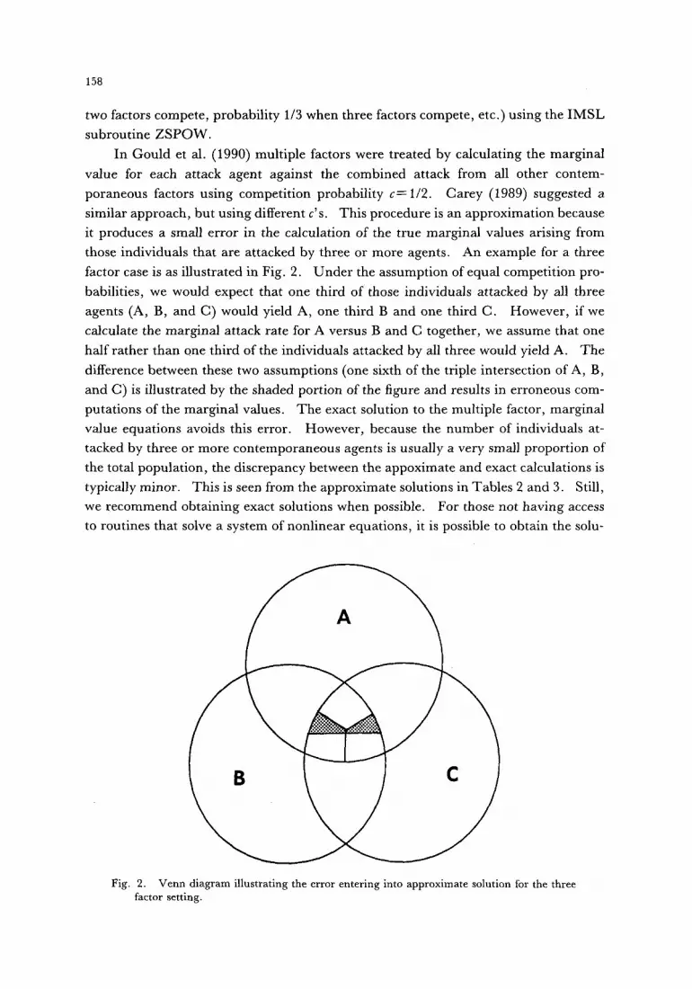
In Gould et al. (1990) multiple factors were treated by calculating the marginal

value for each attack agent against the combined attack from all other contem-

poraneous factors using competit ion probability c = 1/2. Carey (1989) suggested a

similar approach, but using different c's. This procedure is an approximation because

it produces a small error in the calculation of the true marginal values arising from

those individuals that are attacked by three or more agents. An example for a three

factor case is as illustrated in Fig. 2. Under the assumption of equal competit ion pro-

babilities, we would expect that one third of those individuals attacked by all three

agents (A, B, and C) would yield A, one third B and one third C. However , if we

calculate the marginal attack rate for A versus B and C together, we assume that one

half rather than one third of the individuals attacked by all three would yield A. The

difference between these two assumptions (one sixth of the triple intersection of A, B,

and C) is illustrated by the shaded portion of the figure and results in erroneous com-

putations of the marginal values. The exact solution to the multiple factor, marginal

value equations avoids this error. However , because the number of individuals at-

tacked by three or more contemporaneous agents is usually a very small proportion of

the total population, the discrepancy between the appoximate and exact calculations is

typically minor. This is seen from the approximate solutions in Tables 2 and 3. Still,

we recommend obtaining exact solutions when possible. For those not having access

to routines that solve a system of nonlinear equations, it is possible to obtain the solu-

A

s / 1 c

Fig. 2. Venn diagram illustrating the error entering into approximate solution for the three factor setting.

Table 2. Exact and approximate solutions for attack rates with three factors.

Factor Death Rate Exact Approx.

1 .5 .7404 .7298

2 .3 .5181 .5000

3 .1 .2006 .1783

1 .3 .5358 .5000

2 .3 .5358 .5000

3 .3 .5358 .5000

Table 3. Exact and approximate solutions for attack rates with five factors.

Factor Death Rate Exact Approx.

159

1 .30 .3913 .3861

2 .20 .2782 .2762

3 .10 .1485 .1432

4 .05 .0767 .0732

5 .01 .0157 .0149

tion iteratively. On each iteration one solves for each factor versus the rest as in the ap-

proximate solution above, but the c's used are updated based on the solution for the

marginal attack rates at the previous step.

We have not proved that there is always a unique set of acceptable attack rates

which satisfy the equations. However , we have run numerous examples for three,

four and five factor settings under equal competit ion probabilities. In every one of

these cases, though there may be multiple solutions for the system, there has only been

one which is acceptable in that all the values are between 0 and 1. We thus recom-

mend that experimenters use many different starting points in exploring solutions.

With regards to the competit ion probabilities, it is obvious that the experimenter

needs an abundance of information. For example, in the five factor case, there are 49

distinct probabilities that must be specified. It is also clear that an analysis of the sen-

sitivity of the solution to the choice of these probabilities is a much more difficult task

than was given in the two factor settings. This needs further investigation.

STATISTICAL INFERENCE FOR Two FACTORS

We have described how to solve for attack rates given the death rates. In practice

the death rates are estimated from field data and thus are subject to error. Royama

(1981) recognized this but assumed the sample sizes were large enough in order for the

errors in the death rates to be negligible. The second objective of this paper is to ex-

amine some statistical problems associated with making inferences for the marginal at-

tack rates accounting for the sampling error. In particular, we will explore the sampl-

160

ing behavior of the estimated marginal attack rates and develop confidence intervals

and tests of hypotheses.

We begin with two factors, limiting ourselves to the case with a single factor

emerging. Assume that n individuals are observed with A emerging from nn hosts and

B emerging from nB hosts. To address inferences, there must be a model for the data.

We concern ourselves with the simplest scenario in which the n individuals represent a

simple random sample from a single population. Under the above assumption about

the sampling of individuals, one takes da=nn/n and dB=nB/n as the estimated death

rates, where n-~nn + ns. (We employ the common statistical device of using a carat to

distinguish an estimator calculated from the data from the corresponding true but

unknown parameter) . Estimates for the attack rates are obtained as in equation (2)

but with d's replaced by their estimates. The estimated attack rates are denoted ~A

and rhB.

O u r objectives are as follows:

(i) Determine the sampling behavior of the rfi's. In particular, find the mean and the

variance and more generally the approximate distribution for rhA and rhB. As we shall

see, the complicated form of these estimators allows for only approximate results.

(ii) Obtain estimated standard deviations (standard errors) for r~A and rfiB. These pro-

vide measures of precision of the estimates. This can be done in a few different ways.

We consider simple substitutions of estimated values into the approximate standard

deviations and the use of the bootstrap resampling technique.

(iii) Obtain approximate confidence intervals and tests of hypotheses for the marginal

attack rates. We describe two approaches. The first uses the estimated standard

errors and relies on a normal approximation. The second approach is based on the

empirical bootstrap distribution.

The estimated marginal attack rates are nonlinear functions of the estimated

death rates which carries two implications. The first is that the sampling properties of

the estimated attack rates depend on the sampling properties of the estimated death

rates. Secondly, exact properties of the estimated marginal attack rates are difficult to

write down and hence we rely on approximations.

Under the model assumed above, the pair (nA, riB) follows a multinomial distribu-

tion and consequently the joint sampling behavior of dn and a~B is well known; see

Mood, Graybill and Boes (1974). A standard technique, known as the delta method,

is used to obtain approximations for the mean, variances and covariance of the

estimated attack rates; see ApPEnDIX 2. Lett ing Var denote variance, E denote ex-

pected value and Coy denote covariance, the following approximations are obtained.

E(rhA) .w. ma E(rhB) .-~ mB

Var(rhA)~QA/n, Var(rhB)~Q3/n, and Cov(rhA, rhB)~QA#n (7)

where

161

t2mA2dB( 1 -- dB)+ e 2dA(1 -- dA) -- 2 temAdBdA Q'A= n{(c-- I)mB--CmA+ 1} 2

Qs = c2mBZda(1 -- dA) + f2dB(1 -- ds) -- 2cfrnBdAdB n{(c-- 1)mB--cma+ 1} 2

QAB = (1 -- tmB)( tmAdB(1 -- ds) ) -- edAdB + cmB( eda(1 -- dA) -- tmAdadB) n{(c-- 1)ms-- CmA + 1 }2

t = 1 --c, e= 1 --cmA, f-~- 1 - - m s + c m s and ~ means approximately equal to.

The result for the expectations says that the estimates are approximately unbiased

(ignoring terms involving n -2 or smaller). This is also supported by our later in-

vestigations with the bootstrap. These approximations are based on large sample

results and may behave poorly for small samples.

Large sample theory says that for "large" n, rha is approximately normally

distributed with mean mA and variance Var(rhA) as given above. Similarly, rhs is ap-

proximately normal. This provides a succinct description of the sampling behavior

for large sample sizes and also allows us to obtain approximate confidence intervals.

The approximate normality for the distribution of the estimates is illustrated later via the bootstrap analysis.

We note that necessary sample sizes can be determined in a standard way. To

illustrate, suppose the experimenter wants n large enough to be 950//00 sure that the

estimate rhA is within d units of the true value mA. Then (assuming the resulting n is

large enough for the normal approximation to be reasonable) the sample size needed is

n=(1.96)ZQa/d 2. The purpose of giving these details is to note that Qa involves a lot of

information about unknown quantities making apriori sample size computations relatively difficult.

Approximate Confidence Intervals

The above approximations to the variances and covariance involve unknown

parameters and for the purposes of inferences must be estimated. This can be done in

the obvious way by replacing unknown values by their estimates. Denote the square

roots of the estimated variances by SE(rhA) and SE(rhB). These estimated standard

deviations will be referred to as the standard errors for rha and rhs. Large sample

theory suggests that approximate confidence intervals can be obtained via

rhA +--- z~/2SE(rhA) rhB +- z~/2SE(rhB) (8)

where z~/z denotes the appropriate standard normal table value (e.g., for a 95% inter-

val, use z.025----1.96). One can also test hypotheses about the marginal attack rates based on z-tests in a standard way.

162

C o m p a r i n g T w o Rates

Additionally, one may be interested in examining the difference between the two

marginal rates. An estimate of the difference is D=rhA--rhB. The variance of this

est imated difference will involve the covariance between rhA and rhB. Let t ing C denote

the est imated covariance, the s tandard error attached to D is

SE(D) = { (SE(,~B)) 2 + (SE(~B)) 2 -- 2 C} ~:~

A confidence interval for the difference in margina l attack rates is given by D+z~/z

SE(D). A test of the hypothesis H0 : mA = mB can be carried out at level a by rejecting

H0 if 0 is not in the confidence interval. Equivalently one can base the test on the

test statistic Z=D/SE(D) and rejecting H0 if the absolute value of Z is greater than

z~/2. This latter formulat ion allows one to also determine an approximate P-value

(significance level).

I f one is interested in compar ing attack rates for the same agent across two

independent studies, the procedure is similar to the one just described but with no

covariance te rm involved.

Example

T o illustrate, suppose the observed death rates are dA=.6 and dB=.3. The

estimated margina l at tack rates are rha= .8 and rhB=.5, which do not depend on

sample size. Est imated standard errors and approximate confidence intervals are com-

puted following the above developments and are displayed in Table 4 for the cases

where n = 2 0 and n = 1 0 0 . O f course, the s tandard errors decrease as n increases,

resulting in narrower confidence intervals.

Boots t rapping

The procedures described in the preceding sections based on normal approxima-

tions will per form well for reasonable sample sizes. There are other ways to obtain

est imated standard errors which tend to improve on those methods in the presence of

small sample sizes. These include the use of resampl ing plans such as the jackknife

and the bootstrap. These techniques have received considerable at tention lately in

handl ing nonlinear problems in ecological settings; see for example Mueller and

Table 4. Two factor example based on "delta method" with c = 1/2.

Sample Size Factor d rh SE(rh) CI

20 a .6 .8 .1171 (.5705, 1) B .3 .5 .1637 (. 1792, .8209)

100 A .6 .8 .0524 (.6973, .9027) B .3 .5 .0732 (.3565, .6435)

d=observed proportion dying due to factor; rh=estimated marginal attack rate; SE and CI are the estimated standard error and approximate confidence interval from equations (5) and (6).

163

Altenberg (1985), Meyer et al. (1986) and Buonaccorsi and Liebhold (1988). The

bootstrap (see Efron and Tibshirani, 1986) will be examined here. This technique

also allows us to estimate bias and construct approximate confidence intervals.

A total of B bootstrap samples are taken where B is typically large, such as 500 or

1000. F o r j = 1 to B, t h e j t h bootstrap sample consists of the following steps.

a) For i = 1 to n, generate a random quanti ty Xi where Xi = 1 with probability d~

and X i = 2 with probabili ty db.

b) Form dAj = proportion of time that Xi equals and dBj equal the proport ion of

time that Xi equals 2.

c) Obtain solutions for the attack rates using the death rates from b). Denote

these rhAj and rhBj.

What this method does essentially is treat the sample data as if it were the popula-

tion and simulates sampling from it. The result is a set of B solutions for the attack

rates, {(rh~4j, rhBj), j = 1 to B}. The bootstrap sampling is illustrated in Table 5 with

B = 5 0 0 for the two factor example with observed death rates .6 and .3. Each

bootstrap sample takes 20 independent draws where on each draw there is probabilities

.6, .3 and .1 for getting A, B or neither respectively. The first bootstrap sample

resulted in death rates of .6 and .25 respectively producing estimated marginal attack

rates o f . 75 and .4. The last bootstrap sample yielded estimated marginal attack rates

of .8 and .5 which just happens to be the ones obtained from the original data. B

Let mx = Y, ~Aj/B denote the mean of the B bootstrap values and j = 1

B SEB(mA) = {~=l(mAj rnA)2/(B - 1)} '/2

the standard deviation. With respect to Table 3, these are just the mean and standard

deviation of the entries in the third column (rhAj). In a similar fashion, define mB and

SEB(mB). Recall that our estimates obtained from the data are rh~ and rhB. The bootstrap

estimate of the bias of rhA is mA--r hA, while SEB(mA) is the bootstrap estimate of the stan-

dard deviation of rhA. The results for the two factor example with death rates of .6 and

.3 are illustrated in Table 6. There are only modest differences between the estimated

Table 5. Illustration of bootstrap sampling results for two factor example with n=20.

Sample # (j) dAj dsj mxj msj

1 .60 .25 .7500 .4000 2 .55 .25 .6783 .3783

500 .60 .30 .8000 .5000

164

Table 6. Bootstrap analysis oftwo factor exam#e with c=.5.

Sample Size Factor d ~ BMEAN BMED SEB BP BC

20 A .6 .8 .8063 .8000 .1232 (.5362, 1) (.5606, 1)

B .3 .5 .5056 .5000 .1643 (.1834, .8848) (.25, 1)

100 A .6 .8 .8012 .8000 .0528 (.6878, .8986) (.6516, .8994)

B .3 .5 .4950 .5000 .0761 (.3369, .6450) (.3345, .6393)

d=observed proportion dying; ~h=estimated marginal attack rate; BMEAN=bootstrap mean; BMED=bootstrap median; SEB=bootstrap standard error; BP=95~ confidence interval based on per- centile method; BC=95% bias corrected bootstrap interval.

standard errors using the bootstrap method and those in Table 4 from the delta method

even at the smaller sample size. Notice also, the relatively small bootstrap estimates of bias (eg..0063 for factor A when n= 20) which supports the earlier analytical result

which gave an approximate bias of 0.

)__ 0.40 - 0 Z 0.35 W 25) 0.30 O m 0.25 s I.J_ 0.20- Let > O.lS I-- <~ o.10. ._l

w 0.05- (22

o.oo - o.0 o.1

m A

t ~ e n = 2 0

0.2 0,3 0.4 0.5 0.6 0.7 0.8 "0.9 1.0

0 . 4 0 >- i m A (D 0.35. z ~ : ] a n = l O 0

0.30-

O 0.25-

n," L,- 0.20- W

llJl 0.10- W

0 0 0 ! , , ~. fq ~ - 0 0 o , 0 2 0 3 0 4 0 5 0 , o , 0 8 ~ , 0

Fig. 3. Empirical bootstrap distribution of the estimated attack rates for each of the two factors in the two factor example under sample sizes 20 and 100.

165

The empirical boots t rap distribution (EBD) is the distribution of the B boots t rap

values. Figure 3 depicts the EBD for both factors under both sample sizes. These

figures provide an idea of what the sampling distributions look like. Recall that large

sample theory tells us that as n gets large, these distributions will approach a normal

distribution. This is illustrated by figure 3B for n = 100 while for n = 20 (Fig. 3A) there

is some skewness present.

The EBD can also be used to form confidence intervals in several ways. The

easiest is the so-called percentile method. For example, a 95% confidence interval for

rna would use the 2.5th and 97.5th percentile of the EBD. I f the EBD is approximate ly

normal then the percentile method will yield an interval that looks very much like what

would be obtained using (8) but with SE replaced by the boots t rap estimate of s tandard

error. The percentile intervals are presented in Table 6 under the column headed

BP. When the sample size is 20, there is a bit of a difference between these intervals

and the approximate large sample intervals of Table 4, though qualitatively the infor-

mat ion about the margina l at tack rates is not very different.

There are other ways to use the EBD that m a y per form bet ter when the distribu-

tion is asymmetr ic . These are described in detail in Efron and Tibshirani (1986) and

we will not reproduce any details here. We have applied what Efron and Tibshirani

refer to as the BC (bias corrected) method with the results a p p e a r i n g in table 6 under

the column BC. This modification is impor tan t when there is a substantial difference

between the mean and the median (which usually occurs when the distribution is

skewed). For factor B with n = 20 there is a major shift but the other intervals do not

change much.

INFERENCES FOR MANY FACTORS

Though the comput ing becomes more involved, the basic issues and solutions are

the same with more than two factors. As described earlier, we are faced with the ques-

tion of how to describe the precision of the est imated marginal at tack rates. It is pos-

sible to use the delta method, which was employed explicitly in the two factor case, to

obtain approx imate variances and covariances for the est imated marginal at tack rates.

Table 7. Inferences for five factor example assuming equal competition probabilities.

Factor d rh BMEAN BMED SEB BP BC

1 .30 .3913 .3934 .3922 .06125 (.2716, .5075) (.2736, .5094) 2 .20 .2782 .2770 .2765 .05186 (.1810, .3853) (.1817, .3862) 3 .10 .1485 .1520 .1468 .04553 (.0728, .2430) (.0764, .2489) 4 .05 .0767 .0732 .0731 .03038 (.0154, .1336) (.0156, .1336) 5 .01 .0157 .0155 .0156 .01445 (0,.0483) (0,.0477)

d=observed proportion emerging; rh=estimated marginal attack rate; BMEAN=bootstrap mean; BMED=bootstrap median; SEB=bootStrap standard error; CIP=95% confidence interval based on percentile method; BC=95% bias corrected bootstrap interval.

166

While general analytic results are available (APPEm~xx 2), this approach quickly

becomes tedious, both theoretically and computat ional ly, for more than three factors.

As in the two factor case, there is the alternative of bootstrapping. The boots t rap

is carried out in the same m a n n e r as for two factors, except each that for each sample

one must solve for N ra ther than 2 factors.

A boots t rap analysis, with 500 boots t rap samples, was carried out for the five

factor example which was discussed earlier. The data was treated as if it arose form a

sample of n = 100 with results presented in Table 7.

While the boots t rap, and other resampling techniques, provide reasonable

methods of data analysis, they do not provide analytical expressions for variances.

These are helpful both for unders tanding what is contr ibut ing to uncer ta inty and for

sample size determinat ion.

ESTIMATING k-VALUES

T h e k value for a at tack factor is defined by -- log ( i -- m) (Varley and Gradwell ,

1960) where rn is the marginal at tack rate (Royama , 1981) and the log is base 10.

From the inferential s tandpoint , we would like to have a s tandard error to at tach to the

est imated k-value. There are two ways to approach this. One is via the bootstrap,

where we proceed as described earlier, but on each boots t rap sample, after comput ing

the at tack rates one then computes the associated k-values. The s tandard error for the

k-value is then the s tandard deviation over the boots t rap replicates. The other

method, uses s tandard t ransformat ion theory and approximates the s tandard error for

the k-value f rom the s tandard error for the at tack rate and the est imated attack rate.

The relationship is SE(]~)~ SE(rh)/[(1 --rh)2.3026]. Table 8 exhibits est imated k-values

and associated s tandard errors, using both methods, for the five factor example. The

two techniques yield only slight differences.

T h e question of what role the sampling error in the k-values plays in further

analyses, such as density dependence and key-factor analysis (Varley and Gradwell ,

1960), is a very impor tan t one but is well beyond the scope of this paper; see K u n o

(1971, 1973).

Table 8. Estimated k-values and standard errors for five factor example.

Factor k-value SE- T SE-B

1 .2156 .0430 .0445 2 .1416 .0312 .0314 3 .0699 .0232 .0238 4 .0350 .0143 .0143 5 .0070 .0064 .0064

SE-T is standard error using transformation SE-B is standard error obtained from bootstrap

167

DISCUSSION

We have shown that determinat ion of marginal attack rates involves solving a

system of nonlinear equations with the number of equations equal to the number of fac-

tors. An exact solution is given for the two factor case but more than two factors re-

quires iterative techniques.

In order to determine marginal attack rates, information is needed regarding com-

petition probabilites, i.e., the probabilites governing death when factors compete

within the host. In the two factor case it was possible to analytically characterize the

effect of the competit ion rate on the solution (Fig. 1) and it is thus possible to bound the

estimates. With more factors we are faced with difficult problems. Firstly the ex-

per imenter needs information about a potentially large number of probabilities.

Secondly, the ability to assess the dependence of the solutions on the given probabilites

becomes increasingly difficult. One approach is to carry out a sensitivity analysis by

varying these probabilities. We have assumed that the competit ion probabilities (c's)

are known constants and usually that there is equal competition. In principle one

could perform experiments to determine the values for c, but in many cases this infor-

mation will not be available. Fur thermore , the values for c may not be constants at all,

but may vary with environmental conditions or with the t iming of attack of the various

attack agents. In many systems the first agent to attack will be the winner. Thus in

practice one would likely be forced to make simplified assumptions concerning the

values for c. If it is possible to carry out independent experiments to estimate these

c's, the statistical methods can be modified (though this may be complicated with

many factors) to account for the uncertainty in these probabilities.

The statistical methods proposed have been of two types. The so-called delta

method provides approximate variances and covariances for the estimated attack

rates. Estimates of these variances and covariances feed into standard errors and

consequently approximate tests of hypotheses and confidence intervals. The delta

method is cumbersome to employ for three or more factors. The other basic technique

is based on the bootstrap resampling scheme. This provided estimated biases, stand-

ard errors and approximate confidence intervals. It is as easy to apply for five factors

as it is for two (except for the increase in computer time used). With respect to inter-

val estimation it will typically surpass the delta method when the sample sizes are

small. The second method, the bootstrap, especially using the corrected percentile

methods, has broad application though the actual coverage rate of the intervals may

still fall short of the desired goals. However , except for extremely small samples, the

general view provided by bootstrap intervals should be useful. O f course, the problem

will benefit from simulations to evaluate the procedures. Finally, we note that the

delta method has the advantage of providing analytical expressions for variances which

aids in sample size determinat ion as illustrated in the two factor case.

168

SUMMARY

W e p r e s e n t m e t h o d s for so lv ing a n d m a k i n g s ta t i s t ica l in fe rences a b o u t m a r g i n a l

a t t ack ra tes based on o b s e r v e d d e a t h ra tes for c o n t e m p o r a n e o u s m o r t a l i t y factors .

T h e genera l m e t h o d o f so lu t ion involves so lv ing a sys t em of n o n l i n e a r e q u a t i o n s which

d e p e n d in pa r t on c o m p e t i t i o n coeff• tha t express the o u t c o m e w h e n m o r e t h a n

one a g e n t a t t acks the s a m e hos t i n d i v i d u a l . F o r two factors , we p r e se n t a de t a i l ed

ana lys i s of the effect of v a r y i n g this c o m p e t i t i o n coefficient. S ta t i s t ica l in fe rences a re

i l l u s t r a t ed u s i n g s t a n d a r d l a rge s a m p l e a p p r o x i m a t i o n s ( the de l t a m e t h o d ) a n d the

b o o t s t r a p , which is a r e s a m p l i n g t echn ique . W e also ex t end the resul t s to a l low

infe rences for k-values .

ACKNOWLEDGEMENTS: We are grateful to Tom Bellows, Sandy Liebhold and Roy Van Driesche for

reviewing the manuscript and for their helpful comments.

REFERENCES

Bishop, Y. M. M., S. E. Fienberg and P. W. Holland (1975) Discrete Multivariate Analysis. MIT Press:

Cambridge.

Buonaccorsi, J. P. and A. M. Liebhold (1988) Statistical methods for estimating ratios and products in

ecological studies. Environ. Entomol. 17: 572-580.

Carey, J. R. (1989) The multiple decrement life table: a unifying framework for cause-of-death analysis in

ecology. Oecologia 78: 131-137.

Deevy, E. S. (1947) Life tables for natural populations of animals. Quart. Rev. Biol. 22: 283-314.

Efron, B. and R. Tibshirani (1986) Bootstrap methods for standard errors, confidence intervals and other

measures of statistical accuracy. Statistical Science 1: 54-77.

Gould, J. R., J. S. Elkinton and W. E. Wallner (1990) Density dependent suppression of experimentally

created gypsy moth, Lymantria dispar (Lepidoptera: Lymantriidae), populations by natural enemies.

J. Anim. Ecol. 59: 213-233. Kuno, E. (1971) Sampling error as a misleading artifact in 'key factor analysis'. Res. Popul. Ecol. 13: 28-

45. Kuno, E. (1973) Statistical characteristics of the density-independent population fluctuation and the

evaluation of density-dependence and regualtion in animal populations. Res. Popul. Ecol. 15: 99-120.

Meyer, J. S., C. G. Ingersoll, L. L. McDonald and M. S. Boyce (1986) Estimating uncertainty in popula-

tion growth rates: jackknife vs. bootstrap methods. Ecology 67:1156-1166.

Mood, A. M., F.A. Graybill and D. C. Boes (1974) Introduction to the theory of statistics. McGraw-Hill:

New York.

Morris, R. F. (1959) Single factor analysis in population dynamics. Ecology 40: 580-588.

Mueller, L. D. and L. Altenberg (1985) Statistical inference on measures of niche overlap. Ecology 66:

1204-1210.

Royama, T. (1981) Evaluation of mortality factors in insect life table analysis. Ecol. Monogr. 5: 495-505.

Southwood, T. R. E. (1978) Ecological methods with particular reference to the study of insect populations. (2nd

ed.) Ghapman and Hall, London and N.Y.

169

Van Driesche, R. G. (1983) The meaning of "percent parasitism" in studies of insect parasitoids. En-

viron. Entomol. 12: 1611-1622.

Varley, G. Q. and G. R. Gradwell (1960) Key factors in population studies. J. Anita. Ecol. 29: 399-401.

j . P. BUONACCORSl �9 J. S. ELKINTON

~fl-~f[~,~ -v ~'~. ~/~J-~J~fl~l]~., ~.~[~3?s Z 7o ~y~ (delta method) ~ ~ g 7 ~ 6 � 9 ~ ~- 7o J:5~ (bootstrap method) �9 Z ~ ~ ~Y- ~ o "~ ~ ~--J'~]~ ~ ' ~ 7o Y- ~ 'qZ~ l~ ~c. ~- ;~L ~ 0-3 ~fl~[~{~'~] L,

170

APPENDIX 1

Here we provide the general form of the equations relating death rates to marginal attack rates for N

factors. For N factors, we have the following system of N nonlinear equations: for j = 1 to K,

dj= mj I~ (1 -- mj,) + mjY.mq lI(1 -- m~_)c(j Ij, i~) ix 4-j fi iz z

+ rnjZZrni mi II(1 - m i )c(j[j, ix,iz)+mjZY.Zml mi mi 1](1 -mq)c( j [j,ibi2d'3) il i2 1 2 i3 3 il i2 is 1 2 3 i4

. . .etc.

where 1~ denotes a product. There are restrictions on the ranges of the indices in the sums and the pro-

ducts that are not expressed in the above (except for the first product). For example, in the second term of

the expression, the sum over il runs over il from 1 to Nexcep t il ~:j and the product over i2 runs from 1 to N

but i2 must not be equal t o j or il. In general, an indice on a product or sum will run from 1 to N b u t with

the restriction that it not e q u a l j or the indices to the left of it in the expression.

To illustrate, in the three factor case, we have

P(factor 1 emerges)=P(fac tor 1 emerges given only factor 1 was present)P(only factor 1 present)

+P(fac tor 1 emerges given 1 and 2 are present)P(factors 1 and 2 are present)

+P( fac tor 1 emerges given 1 and 3 are present)P(1 and 3 are present)

+P(1 emerges given 1, 2 and 3 are present)P(1, 2 and 3 are present)

= lml ( l - -m2)(1- -m3)+c( l I 1, 2)mlm2(1 - -ms)+c(1 [ 1, 3)mlm3(1--m2)

+c(1 [1, 2, 3)mam2m3.

This simplifies to the first equation in (6).

APPENDIX 2

Here we describe the general method for approximat ing the covariance matrix of the est imated attack

rates for an arbitrary number of factors.

Denote the estimated marginal attack rates by dh, d~2,..., d~N. Let ~ * denote the covariance matrix of

the estimated marginal attack rates. The diagonal elements therefore contain the variances and the off

diagonal elements covariances. Equivalently, the square roots of the diagonal elements of Y,* contain what

are commonly referred to as the s tandard errors. As in the two factor problem, the off diagonal terms are

important when compar ing among the marginal attack rates.

The approximate behavior of the dds is obtained by applying what is referred to as the "delta method"

see Bishop, Fineberg and Hol land (I 975, p.493), and relies on first knowing the sampling properties of the

estimated death rates. Let ~v be the covariance matrix o f t h e esfimated death rates. U n d e r the sampling

scheme assumed, the death rates follow a mulfinomial distribution. Hence, the matrix ~,~ has di(1--di)/n

for the (i , i)th element and --didj/n for the ( i , j ) th element when i-'r

Then an approximation to Y.* is given by

Z * ~ G - 1 Z ~ G - l t

where t denotes matrix transpose. F o r j = 1 to N, write dj=gj(m) where gj(m) simply denotes the function

that defines ~ in terms of ma ... . mN; see APPENDIX 1. The matrix G has as its (j ,k)th element the value

~gj(m)/amk which denotes the partial derivative ofgj(m) with respect to ink.

To illustrate, for the two factor case, we have

and

y, r dA(1--dA)/n - d # J n d=[ - d # J n d~(1 -d~)/~ ]

G = [ 1 + m 8 ( c - 1 ) ma(c-1)

- - C m B 1 - - ( , m A ] '

Forming

Var(rhA Z* = [ t Cov( ~A, ~ )

COV(r~A, ~8) ] ] = G-1ZdG-1t

Var(rh~)

leads to the results in equation 7.

171