Shrinkage Estimation of

Contemporaneous Outliers in

Concurrent Time Series

Nalini Ravishanker*

Department of Statistics

University of Connecticut

Storrs, CT 06269-3120

Lilian S.-Y. Wu

IBM Research Division

Department of Mathematical Sciences

T.J. Watson Research Center

Yorktown Heights, NY 10598

Dipak K. Dey

Department of Statistics

University of Connecticut

Storrs, CT 06269-3120

November 1, 1994

The work of the �rst author was partly supported by a U.S. Army Grant

DAAL03-91-G-0104.

1

Abstract

Contemporaneous outlier blocks (additive or reallocation) caused by spe-

cial events frequently occur in repeated business time series. When the time

series have strong inter-series dependence, shrinkage estimation techniques

provide improved estimates of the time series model parameters and of the

outlier block. A bootstrap estimate of the covariance matrix of the vector of

outlier magnitudes enables us to incorporate the dependence and obtain the

shrinkage estimates.

1 Introduction

American industry is characterized by constant change. Companies intro-

duce new products and reorganize. In this environment of constant change,

historical data on which forecasts are based are often short, comprising usu-

ally of not more than three or four years of monthly data. Frequently, com-

panies are organized into smaller units or divisions and short data series are

available for each division leading to a set of repeated time series. For ex-

ample, in IBM, the division is in terms of geographic areas and short sets

of data on sales of products and revenues are available for each geographic

region. An important characteristic of these repeated series is that they are

de�ned over a common time period and are consequently a�ected by a com-

mon economic and industry environment. This leads to strong inter-regional

dependencies in the data and consequently the estimated model parameters

would be correlated. Further, companies frequently initiate actions such as

price promotions, advertising campaigns or bonuses to sales people. When

such an action is taken, it is critical for a company to obtain an accurate

estimate of the magnitude of the e�ect of the promotional event. This intro-

duces a further similarity between the series through the presence of a block

of anomalous observations in each series at the same known time period - we

refer to this as a contemporaneous outlier block. Within each series, these

outliers could either constitute a continuous block of additive outliers (Mar-

tin, 1989) or a block of reallocation outliers (Wu et al., 1993), the latter

2

being de�ned as a block of additive outliers restricted to sum to zero. It is

of interest in modeling and forecasting, to estimate these contemporaneous

outliers and the parameters of the time series model �tted to the repeated

series as accurately as possible, while incorporating the dependence between

the series.

In this article, we show that shrinkage estimation techniques that account

for cross-sectional dependencies for a moderate number of repeated series

yields large positive improvements for model parameters and the contempo-

raneous outlier magnitudes. Shrinkage estimation for a location parameter

vector from multinormal population has been discussed in the literature, for

example in James and Stein (1961), Berger (1975), Berger and Bock (1976),

Berger et.al. (1977), Berger and Ha� (1983), Brandwein and Strawderman

(1978) and Efron and Morris (1973). Several recent articles on the application

of shrinkage estimation methods to a variety of problems include Blattberg

and George (1991), Garcia-Ferrer et.al. (1987), Greis and Gilstein (1991),

Jorian (1991), Landsman and Damodaran (1989, 1991), Ledolter and Lee

(1993), Thisted and Wecker (1981) and Zellner and Hong (1989).

Section 2 of this article contains a de�nition of contemporaneous outliers

in the framework of Box-Jenkins autoregressive integrated moving average

(ARIMA) modelling. Section 3 describes shrinkage estimation for the con-

temporaneous outlier blocks, incorporating the dependence between the se-

ries. Secton 4 presents as an example, detailed analysis of repeated regional

IBM revenue time series.

2 De�nition of Contemporaneous Outliers

Suppose that each of K concurrent time series fY

i;t

g; i = 1; :::;K belongs

to the class of Box-Jenkins multiplicative seasonal ARIMA models of order

(p; d; q)x(P;D;Q)

s

:

�

i

(B)�

i

(B

s

)(r

d

r

D

s

Y

i;t

� �

i

) = �

i

(B)�

i

(B

s

)a

i;t

(1)

where B is the backward shift operator, r = 1 � B and r

s

= 1 � B

s

are

the nonseasonal and seasonal lag operators respectively, �

i

is the mean of

the ith di�erenced series, �

i

(B) = 1 � �

i;1

B � � � � � �

i;p

B

p

and �

i

(B) =

1� �

i;1

B � � � � � �

i;q

B

q

are polynomials in B of degrees p and q respectively,

3

�

i

(B

s

) and �

i

(B

s

) are polynomials in B

s

of degrees P and Q respectively,

and s is the seasonal period. The a

i;t

are assumed to be independent normally

distributed random variables with mean 0 and variance �

2

i;a

:We assume that

the di�erenced series are stationary and invertible, i.e., that the polynomials

�

i

(z); �

i

(z); �

i

(z

s

) and �

i

(z

s

) have no zeros on or inside the unit circle,

i = 1; :::;K.

Let z

i;t

; t = 1; :::; n; i = 1; :::;K denote observations from the K parallel

time series of interest. We assume that each fz

i;t

g follows an ARIMA model

except for a block of L+1 outliers in each series at times t = c, c+1; :::; c+

L: If these represent contemporaneous blocks of additive outliers, they are

modi�ed as

z

i;t

= Y

i;t

+

L

X

l=0

�

i;l

"

(c+l)

t

t = 1; :::; n; i = 1; :::;K (2)

where "

(r)

t

= 1 if t = r and is 0 otherwise. The �

i;l

; l = 0; :::; L; i = 1; :::;K are

parameters that represent the magnitudes of the anomalies in the underlying

processes fY

i;t

g; occurring in each series at the same successive time points

c; c+ 1; :::; c+ L: If further the �

i;l

are subject to a constraint, such as,

L

X

l=0

�

i;l

= 0; i = 1; :::;K; (3)

we call the z

i;t

; t = c; c+1; :::; c+L; i = 1; :::;K; contemporaneous reallocation

outliers.

The ARIMA model parameters and the �

i;l

in the additive (or realloca-

tion) outlier model may be estimated for each individual time series fz

i;t

g by

the method of maximum likelihood (Wu et al., 1993). This approach, how-

ever, does not take into account the dependence between the series, which

we propose to address through shrinkage estimation.

3 Shrinkage Estimation of Contemporane-

ous Outliers

Let �

�

j

= (�

1;j

; :::; �

K;j

)

0

; j = 1; :::;m; (m = p + q + P + Q + 1); �

l

=

(�

1;l

; :::; �

K;l

)

0

; l = 0; 1; :::; L and

�

�

2

= (�

2

1

; :::; �

2

K

)

0

denote the K-dimensional

4

vectors of the jth ARIMA model parameters, l

th

contemporaneous outlier

magnitudes and residual variances for fz

i;t

g modelled individually by (2.1)

and (2.2). It is well known that asymptotically the maximum likelihood

estimates

b

�

i;j

's and

b

�

i;l

's are normally distributed with corresponding means

�

i;j

's and �

i;l

's. The variances of the

b

�

i;j

's and the

b

�

i;l

's are functions of the

�

i;j

's, �

i;l

's and �

2

i

's respectively.

Following Efron and Morris (1973), a shrinkage estimator of the mean

vector

�

�

of a K-variate (K � 4) normal distribution which dominates the

MLE

x

�

with covariance matrix � = I and under squared error loss is given

component-wise as

e

�

i

=

2

6

6

6

4

1 �

(K � 3)

K

�

j=1

(x

j

� x)

2

3

7

7

7

5

(x

i

� x) + x; i = 1; :::;K (4)

where x = K

�1

K

�

j=1

x

j

: The estimator in (3.1) can be improved by using

the positive-part rule, viz. by setting the quantity in square brackets to be

zero when it would otherwise be negative. If � 6= I; but is a known positive

de�nite matrix, we may reduce the problem to that of � = I by the transfor-

mation w = �

�

1

2

x

�

; obtain the shrinkage estimator of �

�

1

2�

�

using (3.1) and

retransform to get the shrinkage estimator of

�

�

: When � is an unknown ma-

trix, Berger et al. (1977) developed a minimax estimator, provided a random

(KxK) matrix S is available from which � can be estimated independently

of

�

�

:

In time series problems, the covariance matrices of

b

�

�

j

and

b

�

�

l

cannot be

estimated independently, being themselves functions of these parameters.

Hence, we cannot analytically prove that the shrinkage estimator based on

(3.1) (after transformation) does better than the MLE. Thisted and Wecker

(1981) and Landsman and Damodaran (1989, 1991) have, for example, ap-

plied shrinkage estimation to time series model parameters, but only for

situations where this covariance matrix is identity and have justi�ed the

improvement over the MLE by simulation studies which show that the Stein-

type estimators have smaller expected mean squared error than the MLE's

and are on the average closer to the true parameters that the MLE's.

5

3.1. Bootstrap Estimate of Covariance

In order to incorporate the dependence between the repeated series, we

propose a bootstrap estimate of the covariance of the vector of parameter

estimates, as described below. This is natural and has not been discussed

for this problem in the literature.

Let �

j

and

j

denote the covariances of

b

�

�

j

and

b

�

�

l

for j = 1; :::;m and

l = 0; 1; :::; L: We propose that the bootstrap estimate

b

�

j

be constructed as

follows: (i) we recover the (n � p

�

) model residuals

b

a

i;t

from �tting (2.1) -

(2.2) to the data for the ith series (p

�

= p + q + sP + sQ): (ii) let G

n�p

�

(�)

denote the distribution function that assigns mass (n�p

�

)

�1

at each

b

a

i;t

: We

select (n � p

�

) random numbers from the discrete uniform distribution and

obtain bootstrapped errors a

�

i;t

; i = 1; :::;K corresponding to this assignment

for each t = 1; :::; n� p

�

. This generation preserves the correlation structure

that exists between the series. (iii) Given a

�

i;t

; we then generate z

�

i;t

from

(2.1) - (2.2), substituting the MLE's for the true unknown parameters where

necessary. We then obtain the MLE's of �

�

j

and

�

�

l

by �tting (2.1) - (2.2) to

this resampled data z

�

i;t

; repeating this several times (we use 1000 repetitions)

gives a sample of bootstrapped values �

�

i;j

; j = 1; :::;m; �

�

i;l

; l = 0; :::; L

and �

�2

i

; i = 1; :::;K: (iv) The bootstrap estimates

b

�

j

; j = 1; :::;m and

b

l

; l = 0; :::; L are then constructed from the sample covariance matrices of

the samples �

�

i;j

and �

�

i;l

: Bose (1988, 1990) showed that for sample size n,

the distribution of the parameter estimates in autoregressive moving average

models can be bootstrapped with accuracy o(n

�

1

2

) almost surely.

3.2. Shrinkage Estimation Incorporating Inter-series Dependence

The shrinkage estimator of

�

�

l

when the estimated covariance of

�

�

l

is

b

l

, l = 0; :::;L is obtained by transforming

�

�

l

to

�

�

l

=

b

�

1

2

l

�

�

l

, using (3.1)

and transforming back. Shrinkage estimation of �

�

j

; j = 1; :::;m proceeds

similarly. Let �

�

s

j

and

�

�

s

l

denote these shrinkage estimates. We suggest veri-

�cation by simulation that the shrinkage estimator dominates the MLE. We

use two criteria. In terms of

�

�

l

the �rst amounts to checking whether

E

K

X

i=1

(�

s

i;l

� �

i;l

)

2

< E

K

X

i=1

(

b

�

i;l

� �

i;l

)

2

; (5)

6

l = 0; :::; L; i = 1; :::;K; where the expectation is computed by taking the

average (over replication) of the mean squared estimation errors (over series).

The second criterion is the Pitman (1937) nearness criterion;

�

�

s

l

is said to be

Pitman nearer than

b

�

�

l

to the true parameter

�

�

l

if for all

�

�

l

in the parameter

space,

P (j

�

�

s

l

�

�

�

l

j<j

b

�

�

l

�

�

�

l

j) >

1

2

: (6)

The actual implementation of a simulation is discussed in Section 4 in the

content of our illustration.

4 Example

The data that we describe in this article consists of monthly observations

on the revenue of di�erent regional areas in IBM. The revenue data which

consists of 48 observations for each of K = 12 regions is denoted by z

i;t

;

t = 1; :::; 48; i = 1; :::; 12 and is shown in Figure 1. To maintain con�dential-

ity, the exact years are not disclosed and the numbers have all be rescaled

(multiplied) by a constant which we also do not disclose; the rescaling, how-

ever, does not alter the dependence structure in each time series not any

interdependencies between the related series. It is seen that the 12 series

exhibit remarkable similar stochastic patterns (see Figure 2). An interesting

similarity between the data for all 12 regions arises as a consequence of a

sales promotion which produces an anomaly at t = 42 and 43. It is impor-

tant to estimate the magnitude of the net e�ect over these two months as a

result of the sales promotion. The data for these two months will be treated

as a pair of additive outliers. A net e�ect of zero would constitute merely a

reallocation of revenue between the two months (Wu et al., 1993).

We believe that the 12 regional time series may well be modeled by a single

Box-Jenkins model, although the parameter estimates may be expected to

be quite di�erent for the di�erent regions as a consequence of the individual

characteristics of that region. Further, because all the regions are in uenced

by similar macroeconomic factors, there is strong reason to expect that the

revenue data for each region would be correlated with the data for any other

region.

Plots of the sample autocorrelations and partial autocorrelations for the

�rst 41 observations of each region of the revenue data together with 95%

7

marginal con�dence intervals for each correlation coe�cient (Figure 2), and

of the estimated spectral density function (Figure 3) show a strong seasonal

pattern with seasonal period s = 3. This suggests that these data are season-

ally nonstationary. Seasonal di�erencing of period 3 and degree 1 removes

this nonstationarity. The means of the di�erenced series are all close to zero;

we take them as being exactly zero. The autocorrelations, partial autocor-

relations and spectral density function of the di�erenced series show that we

can treat the di�erenced series as stationary. Based on the usual steps in

Box-Jenkins modeling and including model selection criteria such as the AIC

and on residual diagnostics, the model (0; 0; 0) x (3; 1; 0)

3

is seen to be an

acceptable choice as a common single model for the 12 regional revenues:

(�

i;1

; B

3

� �

i;2

B

6

� �

i;3

B

9

)(r

1

3

Y

i;t

) = a

i;t

; i = 1; :::;K: (7)

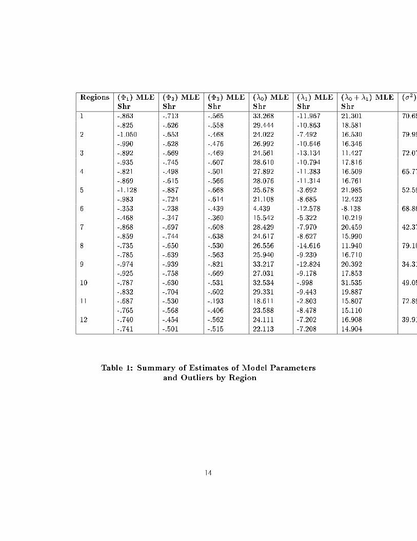
The maximum likelihood estimates

b

�

i;1

;

b

�

i;2

;

b

�

i;3

;

b

�

i;0

;

b

�

i;1

; i = 1; :::;K

are shown in Table 1. These estimates are quite di�erent between the regions.

The �

i;0

's are positive while the �

i;1

's are negative for all the regions. Further,

there is usually a pattern within a block of outliers in business sales or revenue

data. In particular, as a consequence of a promotion (e.g. price reduction,

free gift, or as in this case, a bonus to the salespeople), sales rise during the

promotional period only to fall afterwards below the pre-promotional level.

One quantity of interest in this situation is the sum,

b

�

i;0

+

b

�

i;1

; i = 1; :::;K;

which are also shown in Table 1. It is seen that these are quite di�erent from

zero, leading us to believe that the sales promotion did have a net positive

e�ect.

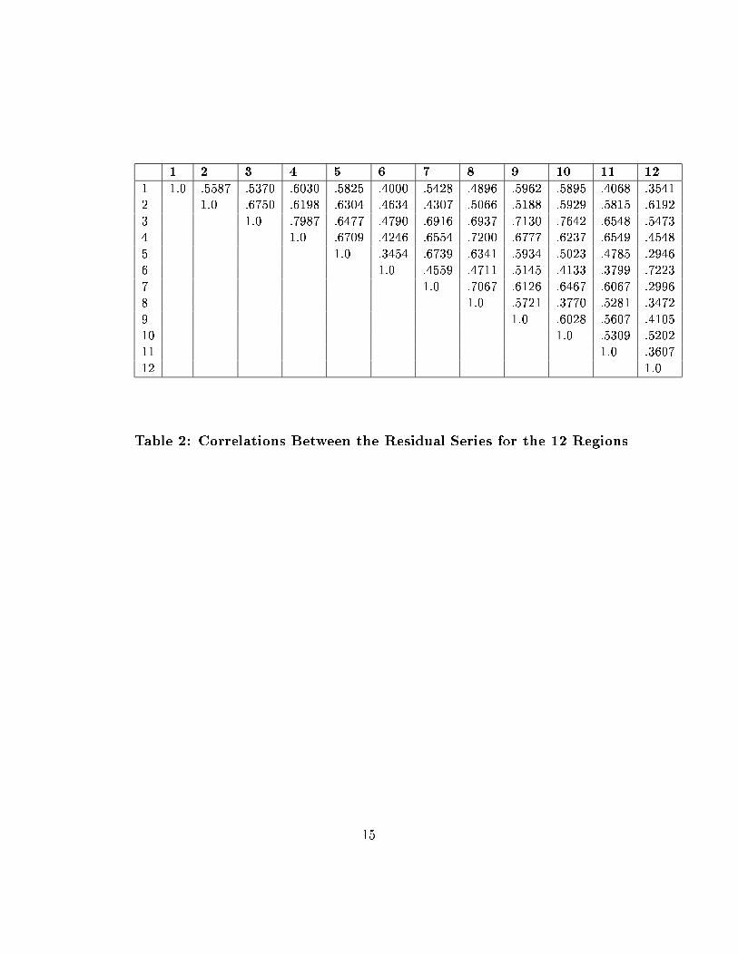
We now turn to shrinkage estimation. To investigate the dependence

structure between the 12 regional data, we compute the product-moment

correlations between the residual series obtained from �tting (2.1) - (2.2) to

each of them. This correlation matrix is shown in Table 2; the presence of

some large correlations strengthens our belief that the dependence structure

between these regional data must be addressed in developing shrinkage esti-

mates. Shrinkage estimates of �

j

and

�

�

l

obtained by the procedure described

in Section 3 are presented in Table 1. We see immediately that there is con-

siderable di�erence between the MLE and shrinkage estimates for �

0

; �

1

and

�

0

+ �

1

: However, as we mentioned earlier, it is not possible to theoretically

verify that the shrinkage estimates perform better than the MLE, hence we

provide results from a simulation study to justify the improvement due to

8

shrinkage for this time series problem.

Our simulation study is based on ten sets of parameter scenarios, ran-

domly generated in the neighborhood of the MLE's of the revenue data.

Speci�cally, we generate ten sets of �

i;j

's, �

i;l

's and �

2

i

's from uniform dis-

tributions on the range between the corresponding minimum and maximum

values for the 12 regions shown in Table 1. We generate the inter-regional

correlation � from a uniform distribution on the range between the mini-

mum and maximum empirical correlation in Table 2. The covariance matrix

between the regions is based on this � and �

2

i

, i = 1; :::; 12 and enables us

to randomly generate a 12-variate normal error vector e

i;t

; t = 1; :::; n from

which the data z

i;t

is computed using the generated �

i;j

's and �

i;l

's. The

MLE's and shrinkage estimates of parameters for this simulated data are

obtained as described in earlier sections and the percentage improvement in

terms of MSE and Pitman nearness is averaged over 500 simulations. The

average percentage improvement over all ten parameter sets in terms of MSE

(Pitman nearness) is 10.10 (56.52) for �

1

; 15.06 (60.50) for �

2

; 18.98 (56.65)

for �

3

; 20.03 (53.58) for

�

�

0

; 26.80 (58.43) for

�

�

1

and 24.61 (57.42) for

�

�

0

+

�

�

1

:

Clearly, the percentage improvement in MSE for the �'s and �'s are posi-

tive and large. Further, the important quantity for assessing whether the

promotion had a positive e�ect as well for estimating the magnitude of the

net e�ect is

�

�

0

+

�

�

1

: Our results show a percentage improvement in MSE

of about 25%, which is large. There is a de�nite advantage in using these

improved estimation techniques for the estimation of model parameters and

outlier magnitudes in these time series models.

References

[1] Berger, J.O. (1975). \Minimax estimation of location vectors for a wide

class of densities", Annals of Statistics 3, 1318-1328.

[2] Berger, J.O. and Bock, M.E. (1976). \Combining independent normal

mean estimation problems with unknown variances", Annals of Statis-

tics 4, 642-648.

[3] Berger, J.O., Bock, M.E., Brown, L.D., Casella, G. and Glesor, L.

(1977). \Minimax estimation of a normal mean vector for arbitrary

9

quadratic loss and unknown covariance matrix". Ann. Statist. 5, 763-

771.

[4] Berger, J.O. and Ha�, L.R. (1983). \A class of minimax estimators of a

normal mean vector for arbitrary quadratic loss and uknown covariance

matrix", Statistics and Decisions 1, 105-129.

[5] Blattberg, R.C. and George, E.I. (1991). \Shrinkage estimation of price

and promotional elasticities: seemingly unrelated equations", Journal

of the American Statistical Association 86, 304-315.

[6] Bose, A. (1988). \Edgeworth correction by bootstrap in autoregres-

sions", Annals of Statistics 16, 1709-1722.

[7] Bose, A. (1990). \Bootstrap in moving average models", Ann. Inst.

Statist. Math., 42, 753-768.

[8] Box, G.E.P. and Jenkins, G.M. (1976). Time Series Analysis: Forecast-

ing and Control. Holden Day: San Francisco.

[9] Brandwein, A.C. and Strawderman, W.E. (1978). \Minimax estimation

of location parameters for spherically symmetric unimodal distributions

under quadratic loss", Annals of Statistics 6, 377-416.

[10] Bruce, A.G. and Martin, R.D. (1989). \Leave-k-out diagnostics for time

series", Journal of the Royal Statistical Society, B 51, 363-424.

[11] Efron, B. and Morris, C. (1973). \Combining possibly related estimation

problems", Journal of the Royal Statistical Society, B 35, 379-402.

[12] Garcia-Ferrer, A., High�eld, R.A., Palm, F. and Zellner, A. (1987).

\Macroeconomic forecasting using pooled international data", Journal

of Business and Economic Statistics, 5, 53-67.

[13] Gleser, L.J. (1979). \Minimax estimation of a normal mean vector when

the covariance matrix is unknown", Annals of Statistics 7, 838-846.

[14] Greis, N.P. and Gilstein, C.Z. (1991). \Empirical Bayes methods for

telecommunications forecasting", International Journal of Forecasting

7, 183-197.

10

[15] James, W. and Stein, C. (1961). \Estimation with quadratic loss", Proc.

Fourth Berkeley Symposium in Math. Statist. Prob. 1, 361-380. Univer-

sity of California Press.

[16] Jorian, P. (1991). \Bayesian and CAPM estimators of the means: Im-

plications for portfolio selection", Journal of Banking and Finance 15,

717-727.

[17] Keating, J.P. (1985). \Pitman's measure of closeness", Sankhya, B 47,

22-32.

[18] Landsman, W.R. and Damodaran, A. (1989). \Using shrinkage estima-

tions to improve upon time-series model proxies for the security market's

expectation of earnings", Journal of Accounting Research 27, 97-115.

[19] Landsman, W.R. and Damodaran, A. (1991).\A comparison of quarterly

earnings per share forecasts using James-Stein and unconditional least

squares parameter estimators", International Journal of Forecasting 5,

491-500.

[20] Ledolter, J. and Lee, C.S. (1993). \Analysis of many short time se-

quences: forecast improvements achieved by shrinkage", Journal of Fore-

casting, 12, 1-11.

[21] Pitman, E.J.G. (1937). \The closest estimates of statistical parameters",

Proceedings of the Cambridge Philosophical Society 33, 212-222.

[22] Sen, P.K. (1986). \Are ban estimators the Pitman-closest ones too?",

Sankhya, A 48, 51-58.

[23] Thisted, R.A. and Wecker, W.E. (1981). \Predicting a multitude of time

series", Journal of the American Statistical Association 76, 516-523.

[24] Wu, L. S.-Y., Hosking, J.R.M. and Ravishanker, N. (1993). \Realloca-

tion outliers in time series", Applied Statistics, 42, 301-313.

[25] Zellner, A. and Vandaale, N. (1974). \Bayes-Stein estimators for K-

means regression and simultaneous equation models". In: Studies in

Bayesian Econometrics and Statistics, S. Fienberg and A. Zellner (Eds.),

North Holland: Amsterdam.

11

[26] Zellner, A. and Hong, C. (1989). \Forecasting international growth rates

using Bayesian shrinkage and other procedures". Journal of Economet-

rics, 40, 183-202.

12

List of Figures and Tables

Figure 1: IBM regional revenue data for 12 regions.

Figure 2: Sample autocorrelations for the IBM regional revenue data.

Table 1: Summary of estimates of model parameters and outliers by

region.

Table 2: Correlations between the residual series for the 12 regions.

13

Regions (�

1

) MLE (�

2

) MLE (�

3

) MLE (�

0

) MLE (�

1

) MLE (�

0

+ �

1

) MLE (�

2

) MLE

Shr Shr Shr Shr Shr Shr

1 -.863 -.713 -.565 33.268 -11.967 21.301 70.656

-.825 -.626 -.558 29.444 -10.863 18.581

2 -1.050 -.653 -.468 24.022 -7.492 16.530 79.991

-.990 -.628 -.476 26.992 -10.646 16.346

3 -.892 -.669 -.469 24.561 -13.134 11.427 72.072

-.935 -.745 -.607 28.610 -10.794 17.816

4 -.821 -.498 -.501 27.892 -11.383 16.509 65.775

-.869 -.615 -.566 28.076 -11.314 16.761

5 -1.128 -.887 -.668 25.678 -3.692 21.985 52.595

-.983 -.724 -.614 21.108 -8.685 12.423

6 -.353 -.238 -.439 4.439 -12.578 -8.138 68.861

-.468 -.347 -.360 15.542 -5.322 10.219

7 -.868 -.697 -.608 28.429 -7.970 20.459 42.373

-.859 -.744 -.638 24.617 -8.627 15.990

8 -.735 -.650 -.530 26.556 -14.616 11.940 79.109

-.785 -.639 -.563 25.940 -9.230 16.710

9 -.974 -.939 -.821 33.217 -12.824 20.392 34.311

-.925 -.758 -.669 27.031 -9.178 17.853

10 -.787 -.630 -.531 32.534 -.998 31.535 49.056

-.832 -.704 -.602 29.331 -9.443 19.887

11 -.687 -.530 -.193 18.611 -2.803 15.807 72.895

-.765 -.568 -.406 23.588 -8.478 15.110

12 -.740 -.454 -.562 24.111 -7.202 16.908 39.911

-.741 -.501 -.515 22.113 -7.208 14.904

Table 1: Summary of Estimates of Model Parameters

and Outliers by Region

14

1 2 3 4 5 6 7 8 9 10 11 12

1 1.0 .5587 .5370 .6030 .5825 .4000 .5428 .4896 .5962 .5895 .4068 .3541

2 1.0 .6750 .6198 .6304 .4634 .4307 .5066 .5188 .5929 .5815 .6192

3 1.0 .7987 .6477 .4790 .6916 .6937 .7130 .7642 .6548 .5473

4 1.0 .6709 .4246 .6554 .7200 .6777 .6237 .6549 .4548

5 1.0 .3454 .6739 .6341 .5934 .5023 .4785 .2946

6 1.0 .4559 .4711 .5145 .4133 .3799 .7223

7 1.0 .7067 .6126 .6467 .6067 .2996

8 1.0 .5721 .3770 .5281 .3472

9 1.0 .6028 .5607 .4105

10 1.0 .5309 .5202

11 1.0 .3607

12 1.0

Table 2: Correlations Between the Residual Series for the 12 Regions

15